Towards non-Hermitian quantum statistical thermodynamics

Abstract

Non-Hermitian Hamiltonians possessing a discrete real spectrum motivated a remarkable research activity in quantum physics and new insights have emerged. In this paper we formulate concepts of statistical thermodynamics for systems described by non-Hermitian Hamiltonians with real eigenvalues. We mainly focus on the case where the energy and another observable are the conserved quantities. The notion of entropy and entropy inequalities are central in our approach, which treats equilibrium thermodynamics.

1 Introduction

Entropy is a fundamental concept in science, with origin in thermodynamics. This branch of physics has been founded almost 200 years ago and its conceptual bases remained unchanged until now. The realm of thermodynamics has been considerably extended, from dealing with macroscopic systems, to individual quantum systems and black holes. Jaynes, in 1957, revisited the formulation of thermodynamics for an arbitrary number of conserved quantities, through the maximum entropy principle [11]. This principle demands the following. Consider a given system and specified constraints on its conserved properties, which, necessarily, are always very far from uniquely determining the macroscopic state of the system. This state is obtained, according with the well known Boltzmann prescription, by considering only the microstates (in the sense of analytical mechanics) which are compatible with the constraints, and by assigning equal probability to each one of them. The described procedure is often simplified by replacing the exact constraints by the respective average values for a certain statistical population. It is well known that the relative statistical error involved in this simplification is of the order of the inverse of the square root of the number of particles of the system. The maximum entropy principle states that the probability distribution which better represents the equilibrium state is the one which maximizes the entropy, under imposed average values of certain conserved quantities, i.e., constants of motion.

In the last decades, the consideration, in quantum physics, of non-Hermitian Hamiltonians with a real discrete spectrum, gave rise to an intense research activity in physics and mathematics, see e.g., [1, 2, 6, 9, 14, 15, 16, 17]. In this note, the maximum entropy principle is formulated for systems described by the non-Hermitian Hamiltonian $H$ with a real discrete spectrum. We focus on the extension, for this setup, of classical results of thermodynamics, namely, a fundamental inequality which reflect the second law, and related topics [3, 4, 18]. As a starting point, we reinterpret some of the standard thermodynamic quantities in the non-Hermitian context.

We propose a formulation of equilibrium statistical thermodynamics in this framework. We assume that $H$ is defined in a Hilbert space $\cal H$ with inner product $\langle\cdot,\cdot\rangle$. In this space, a new inner product is introduced in order to preserve the standard probabilistic interpretation of quantum mechanics. The new inner product also plays a crucial role in our formulation of quantum statistical thermodynamics, which recovers results for the usual Hermitian set up.

We mostly concentrate in the scenario of two conserved quantities. This captures the physics contained in the general case of $k$ conserved quantities. Consider the thermal state of a system with Hamiltonian $H$ and a conserved observable $K$ (i.e., $[K,H]=KH-HK=0$), described by the density matrix $\rho$. Its energy and $K$ expectation values are given, respectively, by $\langle H\rangle={\rm Tr}H\rho$ and $\langle K\rangle={\rm Tr}K\rho.$ There are many thermal states, (also known as mixed states), with this average energy and $K$ expectation value, and the thermal equilibrium state is the one which maximizes the von Neumann entropy $S_{\rho}=-{\rm Tr}\rho\log\rho,$ subject to the considered expectation values of the energy and of $K$.

There are two ways to obtain the equilibrium thermal state: by maximizing the entropy, and in this case the inverse temperature is the Lagrange multiplier which fixes the energy, or by minimizing the free energy, and then the absolute temperature characterizes the associated heat source. More generally, in the first case, the system is isolated and the parameters playing the role of the Lagrange multipliers, which control the conserved quantities, $H$ and $K$, are fixed in such a way as to preserve the values of these quantities. In the second case, the system is not isolated and the corresponding parameters characterize the sources of the conserved quantities, which interact with the system.

The article is organized as follows. In Section 2, useful prerequisites are presented. In Section 3, our proposed formalism for the non-Hermitian context is given. In Section 4, the maximum entropy principle is investigated. In Section 6, our conclusions are summarized, and the difficulties of an extension to the infinite dimensional context are sketched.

2 Prerequisites

The von Neumann formalism of quantum statistical physics is established in the language of Hilbert spaces. Quantum observables are self-adjoint (synonymously, Hermitian) operators acting on a Hilbert space $\cal H$. We denote by $H_{n}$ the set f $n\times n$ Hermitian matrices. A density matrix is a positive semidefinite matrix with unit trace. Density matrices with rank 1 describe pure states, while those with rank greater than 1 describe mixed states of the system. Quantum probability measures are described by the eigenvalues of density matrices.

The statistical expectation value, or average value, of the observable $A$ for the state $\rho$ is given by

$$\langle A\rangle_{\rho}={\rm Tr}(A\rho),$$

and the von Neumann entropy is equal to

$$S_{\rho}=-{\rm Tr}(\rho\leavevmode\nobreak\ \log\rho)=-\sum_{k}\eta_{k}\log\eta_{k},$$

where the $\eta_{k}$ are the eigenvalues of $\rho$. By convention, $0\log 0=0.$

Gibbs states describe the equilibrium states of classical thermodynamics. They maximize the entropy $S_{\rho}$ under the condition $E={\rm Tr}(H\rho)$, and minimize $E$ for fixed entropy $S_{\rho}$.

Let $A_{i},\leavevmode\nobreak\ i=1,\ldots,n$ be Hermissian matrices and assume that $\left\{{\bf 1},A_{1},\ldots,A_{n}\right\}$ are linearly independent, where ${\bf 1}$ is the identity matrix. A generalized thermal equilibrium state is described by a density matrix of the form

$$\rho_{\beta}=\frac{\mathrm{e}^{-(\beta_{1}A_{1}+\ldots+\beta_{n}A_{n})}}{{\rm Tr}{\mathrm{e}^{-(\beta_{1}A_{1}+\ldots+\beta_{n}A_{n})}}},\quad\beta_{1},\ldots,\beta_{n}\in\mathbb{R}.$$

The Hermitian matrices $A_{i}$ represent conserved quantities, that is to say, the Hamiltonian or observables that commute with it, and the $\beta_{i}$ may be regarded as generalized inverse temperatures associated to the conserved quantities. The function

$$Z:={\rm Tr}{\mathrm{e}^{-(\beta_{1}A_{1}+\ldots+\beta_{n}A_{n})}}$$

is the generalized partition function [20] and $\log Z$ is the log partition function.

Consider the Gibbs state $\rho_{\beta}$. The exponential family ${\cal E}=\{\rho_{\beta}:\beta\in\mathbb{R}^{n}\}$ has two natural charts. The first chart is the inverse map to

$$\alpha:\mathbb{R}^{n}\rightarrow,{\cal E},\quad\beta\rightarrow\rho_{\beta},$$

so that the chart is $\alpha^{-1}:{\cal E}\rightarrow\mathbb{R}^{n}.$ The second chart is the restriction to $\cal E$ of the linear map

$$\mathbb{E}:H_{n}\rightarrow\mathbb{R}^{n},\quad B\rightarrow{\rm Tr}(BA_{i})_{i=1}^{n},$$

i.e., the chart is $\mathbb{E}_{\cal E}\rightarrow\mathbb{R}^{n}.$ Recall that $\alpha^{-1}({\cal E})=\mathbb{R}^{n}$ and that $\mathbb{E}({\cal E})={\rm int}(W(A_{1},\ldots,A_{n}))$, the interior of the joint numerical range of the matrices $A_{1},\ldots,A_{n},$ which is defined as

$$W(A_{1},\ldots,A_{n})=\{\langle A_{1},\ldots,A_{n})\psi,\psi\rangle:\psi\in{\cal H},\leavevmode\nobreak\ \langle\psi,\psi\rangle=1\}.$$

It is well-known that ${\cal E}\circ\alpha:\mathbb{R}^{n}\rightarrow{\rm int}(W(A_{1},\ldots,A_{n}))$ is an analytic diffeomorphism [19, 20].

Let us consider the set

$$\Omega_{\beta_{0}}:=\left\{{\rm Tr}\left((A_{1},\ldots,A_{n})\frac{\mathrm{e}^{-\beta_{1}A_{1}-\ldots-\beta_{n}A_{n}}}{{\rm Tr}\leavevmode\nobreak\ \mathrm{e}^{-\beta_{1}A_{1}-\ldots-\beta_{n}A_{n}}}\right):\sqrt{\beta_{1}^{2}+\ldots+\beta_{n}^{2}}\leq\beta_{0};\leavevmode\nobreak\ \beta_{1},\ldots,\beta_{n}\in\mathbb{R}\right\},$$

Its boundary $\partial\Omega_{\beta_{0}}$ is an analytic hypersurface in $\mathbb{R}^{n}.$ For $\beta^{\prime}_{0}<\beta_{0}$, we have

$$\Omega_{\beta^{\prime}_{0}}\subset\Omega_{\beta_{0}}.$$

It should be noticed that $\Omega_{\beta_{0}}$ is convex.

3 Non-Hermitian formalism

Assume by now that $\cal H$ has finite dimension $n$. The operator $H$, which is assumed to have real discrete spectrum, and its adjoint $H^{\dagger}$ have the same eigenvalues. We denote by $\psi_{i}$ the eigenvector of $H$ associated to the (non degenerate) eigenvalue $\lambda_{i}$, and by $\widetilde{\psi}_{i}$ the eigenvector of $H^{\dagger}$ associated to the same eigenvalue $\lambda_{i}$. The sets of eigenvectors $\left\{\psi_{k}\right\}$ and $\left\{\widetilde{\psi}_{k}\right\}$ are biorthogonal, $\langle\psi_{k},\widetilde{\psi}_{l}\rangle=0$ if $k\neq l$, and form bases of $\cal H$, since this space has a finite dimension $n$. We orthonormalize the bases $\{\psi_{i}\},\leavevmode\nobreak\ \{\widetilde{\psi}_{i}\},$ so that

$$\langle\psi_{k},\widetilde{\psi}_{l}\rangle=\delta_{kl},$$

where $\delta_{kl}$ denotes the Kronecker symbol (=1 for $k=l$ and 0 otherwise). Let us define the matrix $D=[D_{ij}]_{i,j=1}^{n}$ (we use synonymously the terms operator and matrix) such that

$$\widetilde{\psi}_{i}=D\psi_{i},\leavevmode\nobreak\ \leavevmode\nobreak\ i=1,\ldots,n.$$ (1)

Proposition 3.1

The matrix $D$ is positive definite.

Proof. For $\psi=\sum_{k=1}^{n}x_{k}\psi_{k}$, we have

$$\langle D\psi,\psi\rangle=\sum_{k,l=1}^{n}\langle D\psi_{k},\psi_{l}\rangle x_{k}\overline{x}_{l}=\sum_{k,l=1}^{n}\langle\widetilde{\psi}_{k},\psi_{l}\rangle x_{k}\overline{x}_{l}=\sum_{k,l=1}^{n}\delta_{kl}x_{k}\overline{x}_{l}=\sum_{k=1}^{n}|x_{k}|^{2}\geq 0,$$

and is zero if and only if $\psi=0.$   

We define a new inner product

$$\langle\phi,\psi\rangle_{D}:=\langle D\phi,\psi\rangle,\leavevmode\nobreak\ \leavevmode\nobreak\ \text{for any}\leavevmode\nobreak\ \leavevmode\nobreak\ \phi,\leavevmode\nobreak\ \psi\in{\cal H}.$$

For commodity, we say that this is the inner product with metric $D$, or simply the $D$-inner product.

Proposition 3.2

The non-Hermitian Hamiltonian $H$ is Hermitian relatively to the $D$-inner product.

Proof. For any $\psi=\sum_{k=1}^{n}x_{k}\psi_{k}$ in $\cal H$ we have,

$$\langle DH\psi,\psi\rangle\in\mathbb{R},$$

because

$$\langle DH\psi,\psi\rangle=\sum_{k,l=1}^{n}\langle DH\psi_{k},\psi_{l}\rangle x_{k}\overline{x}_{l}=\sum_{k,l=1}^{n}\lambda_{k}\langle\widetilde{\psi}_{k},\psi_{l}\rangle x_{k}\overline{x}_{l}$$

$$=\sum_{k,l=1}^{n}\lambda_{k}\delta_{kl}x_{k}\overline{x}_{l}=\sum_{k=1}^{n}\lambda_{k}|x_{k}|^{2}\in\mathbb{R}.$$

Thus,

$$\langle H\psi,\psi\rangle_{D}=\langle DH\psi,\psi\rangle=\langle H^{\dagger}D\psi,\psi\rangle=\langle D\psi,H\psi\rangle=\langle\psi,H\psi\rangle_{D}.$$

 

Proposition 3.3

The non-Hermitian Hamiltonian $H$ has real eigenvalues if and only if there exists a positive definite matrix $D_{0}$ such that

$$D_{0}H=H^{\dagger}D_{0}.$$

Proof. Consider $D_{0}=D$ above defined. Observe that from Proposition 3.2 it follows that

$$\langle DH\psi,\psi\rangle=\langle D\psi,H\psi\rangle=\langle H^{\dagger}D\psi,\psi\rangle,$$

for any $\psi\in{\cal H}$ so that $DH=H^{\dagger}D.$

Suppose next that there exists $D_{0}$ positive definite and $D_{0}H=H^{\dagger}D_{0}.$ Let $\psi_{k}$ be an eigenvector of $H$ associated with the eigenvalue $\lambda_{k}$, claimed to be real, that is $H\psi_{k}=\lambda_{k}\psi_{k}$, so that

$$D_{0}H\psi_{k}=H^{\dagger}D_{0}\psi_{k}=\lambda_{k}D_{0}\psi_{k}.$$ (2)

Since

$$\lambda_{k}=\frac{\langle\psi_{k}D_{0}H,\psi_{k}\rangle}{\langle D_{0}\psi_{k},\psi_{k}\rangle}=\frac{\langle\psi_{k}H^{\dagger}D_{0},\psi_{k}\rangle}{\langle D_{0}\psi_{k},\psi_{k}\rangle},$$

it follows that $\lambda_{k}$ is real.   

Proposition 3.4

The Hamiltonian $H$ is similar to a Hermitian operator $H_{0}$, under the similarity $D^{1/2}H{D^{-1/2}}.$

Proof. The condition $DH=H^{\dagger}D$ implies that

$$D^{1/2}HD^{-1/2}=D^{-1/2}H^{\dagger}{D^{1/2}}=H_{0}.$$

Thus, $H_{0}$ is Hermitian and

$$H=D^{-1/2}H_{0}{D^{1/2}}.$$

 

Suppose that the statistical properties of the physical system we are concerned are described by a density matrix $\rho$, with ${\rm Tr}\rho=1,$ which is positive semidefinite (notation, $\rho\geq 0$) under the metric $D$,

$$\langle\rho\psi,\psi\rangle_{D}=\langle D\rho\psi,\psi\rangle\geq 0,\leavevmode\nobreak\ \leavevmode\nobreak\ \text{ for any}\leavevmode\nobreak\ \leavevmode\nobreak\ \psi\in{\cal H},$$

so that $D\rho=\rho^{\dagger}D.$ The statistical expectation value of the energy is $\langle H\rangle={\rm Tr}(H\rho)$ and the entropy is $S_{\rho}=-{\rm Tr}(\rho\log\rho).$ We define the (non-equilibrium) free energy of the system as in the standard case,

$$F={\rm Tr}(H\rho)+{\rm Tr}(\rho\log\rho).$$ (3)

Notice that these definitions, used in the standard Hermitian set up, are still meaningful in the present context. In fact, since $DH=H^{\dagger}D$ and $D\rho=\rho^{\dagger}D$, we have, by the ciclicity of the trace,

$${\rm Tr}(\rho H)={\rm Tr}(D\rho HD^{-1})={\rm Tr}(\rho^{\dagger}DHD^{-1}={\rm Tr}(\rho^{\dagger}HDD^{-1})={\rm Tr}(H^{\dagger}\rho^{\dagger})\in\mathbb{R}.$$

Similarly,

$${\rm Tr}(\rho\log\rho)={\rm Tr}(D\rho\log\rho D^{-1})={\rm Tr}(\rho^{\dagger}\log\rho^{\dagger}DD^{-1})={\rm Tr}(\rho^{\dagger}\log\rho^{\dagger})\in\mathbb{R}.$$

The free-energy is related to the partition function as follows

$$F=-T\log\leavevmode\nobreak\ Z.$$

The first law of thermodynamics means that the energy is an additive state function which is conserved, i.e., it remains constant. The energy expectation value is

$$\langle H\rangle=-\frac{{\rm d}\log Z}{{\rm d}\beta}=\frac{{\rm Tr}H\mathrm{e}^{-\beta H}}{{\rm Tr}\mathrm{e}^{-\beta H}}.$$

The second law of thermodynamics means that the entropy is an additive state function which increases when equilibrium is approached. The entropy is

$$S=\frac{{\rm d}}{{\rm d}T}(T\log Z)=\log Z+\beta\frac{{\rm Tr}H\mathrm{e}^{-\beta H}}{{\rm Tr}\mathrm{e}^{-\beta H}}=-{\rm Tr}\left(\frac{\mathrm{e}^{-\beta H}}{{\rm Tr}\mathrm{e}^{-\beta H}}\log\frac{\mathrm{e}^{-\beta H}}{{\rm Tr}\mathrm{e}^{-\beta H}}\right),$$

where $T=1/\beta.$

Consider next the existence of a conserved quantity $K$, that is, an observable with real eigenvalues, which, be definition, commutes with $H$, $[H,K]=0.$ Thus, $H$ and $K$ have common eigenvectors, so that they are both $D$-Hermitian, and we have $DH=H^{\dagger}D$ and $DK=K^{\dagger}D.$ If, moreover, $\beta,\leavevmode\nobreak\ \zeta\in\mathbb{R},$ the equilibrium statistical expectation values of $H$ and $K$ may be defined as

$$\langle H\rangle=\frac{{\rm Tr}H\mathrm{e}^{-\beta H-\zeta K}}{{\rm Tr}\mathrm{e}^{-\beta H-\zeta K}},\leavevmode\nobreak\ \leavevmode\nobreak\ \text{and}\leavevmode\nobreak\ \leavevmode\nobreak\ \langle K\rangle=\frac{{\rm Tr}K\mathrm{e}^{-\beta H-\zeta K}}{{\rm Tr}\mathrm{e}^{-\beta H-\zeta K}},$$

because ${{\rm Tr}H\mathrm{e}^{-\beta H-\zeta K}},\leavevmode\nobreak\ {{\rm Tr}K\mathrm{e}^{-\beta H-\zeta K}},\leavevmode\nobreak\ {{\rm Tr}\mathrm{e}^{-\beta H-\zeta K}}\in\mathbb{R}.$ In fact, as $D>0,$ $DH=H^{\dagger}D,$ $DK=K^{\dagger}D,$ we have

$${\rm Tr}(\beta H+\zeta K)={\rm Tr}D(\beta H+\zeta K)D^{-1}={\rm Tr}(\beta H+\zeta K)^{\dagger}DD^{-1}={\rm Tr}(\beta H+\zeta K)^{\dagger}.$$

We easily find

$${\rm Tr}(\beta H+\zeta K)^{k}={\rm Tr}(D(\beta H+\zeta K)^{k}D^{-1})={\rm Tr}((\beta H^{\dagger}+\zeta K^{\dagger})D(\beta H+\zeta K)^{(k-1)}D^{-1})$$

$$=\ldots={\rm Tr}(({\beta H^{\dagger}+\zeta K^{\dagger}})^{k}DD^{-1})={\rm Tr}{(\beta H^{\dagger}+\zeta H^{\dagger})}^{k}.$$

Since

$$\mathrm{e}^{-\beta H-\zeta K}=\sum_{k=0}^{\infty}\frac{(-\beta\leavevmode\nobreak\ H-\zeta K)^{k}}{k!},$$

the claim follows.

According to the maximum entropy (MaxEnt) principle, the equilibrium thermal state of an isolated system is determined by maximizing the entropy of the system subject to constrained values of the conserved quantities $H$ and $K$. The Lagrange multipliers which control the conserved quantities are fixed in such a way as to preserve their values.

Proposition 3.5

If $H$ and $K$ are $D$-Hermitian, $\beta,\leavevmode\nobreak\ \zeta\in\mathbb{R},$ and $[H,K]=0,$ then

$$\langle H\rangle=\frac{-\partial\log Z}{\partial\beta},$$

and

$$\langle K\rangle=\frac{-\partial\log Z}{\partial\zeta}.$$

Proof. Since $[H,K]=0$, we may write

$$\frac{{\rm Tr}H\mathrm{e}^{-\beta H-\zeta K}}{{\rm Tr}\mathrm{e}^{-\beta H-\zeta K}}=\frac{-\partial\log Z}{\partial\beta},$$

and

$$\frac{{\rm Tr}K\mathrm{e}^{-\beta H-\zeta K}}{{\rm Tr}\mathrm{e}^{-\beta H-\zeta K}}=\frac{-\partial\log Z}{\partial\zeta}.$$

The result follows.   

The following question naturally arises. Is it legitimate to describe an isolated system by a Gibbs state? We try to provide a partial answer to it. Let us replace the Hilbert space $\cal H$ by

$${\cal H}_{comp}={\cal H}\otimes{\cal H}\otimes\ldots\otimes{\cal H},$$

where the number of factors in the tensorial product is $N$, and let us consider the composed system which is constituted by $N$ partial systems and is described by the Hamiltonian

$$H_{comp}=H\oplus H\oplus\ldots\oplus H,$$

where the number of summands is $N$. For simplicity, we simply denote by $H$, according to its position in the direct sum, each one of the operators $(H\otimes I\otimes\ldots\otimes I),\leavevmode\nobreak\ \leavevmode\nobreak\ (I\otimes H\otimes I\otimes\ldots\otimes I),\leavevmode\nobreak\ \leavevmode\nobreak\ \ldots,\leavevmode\nobreak\ \leavevmode\nobreak\ (I\otimes I\otimes\ldots\otimes I\otimes H)$ acting on ${\cal H}_{comp}$. It is clear that the energy expectation value, free energy, entropy and energy variance of the composed system are $N$ times the corresponding quantities relative to the partial system. Since the statistical error is determined by the square root of the variance, it is clear that, if $N$ is large enough, the Gibbs state safely describes the isolated composed system.

4 MaxEnt principle

The following minimum free energy (or maximum entropy) inequality holds.

Theorem 4.1

Let the Hamiltonian $H$ be non-Hermitian with real simple eigenvalues. Assume $D$ as defined in (1) and $\beta,\zeta\in\mathbb{R}$. If the density matrix $\rho$ and the operator $K$ are Hermitian relatively to the $D$-inner product, then

$$-\log{\rm Tr}\mathrm{e}^{-\beta H-\zeta K}\leq{\rm Tr}\rho(\beta H+\zeta K+\log\rho),$$ (4)

with equality occurring if and only if

$$\rho=\rho_{0}:={\mathrm{e}^{-\beta H-\zeta K}\over{\rm Tr}\mathrm{e}^{-\beta H-\zeta K}}.$$ (5)

Proof. According to the hypothesis, $\rho$ and $D$ satisfy $D\rho=\rho^{\dagger}D,\leavevmode\nobreak\ \leavevmode\nobreak\ DK=K^{\dagger}D$. Let the matrix $U$ satisfy

$$\langle DU\psi,U\psi\rangle=\langle D\psi,\psi\rangle,$$

for all $\psi\in{\cal H}.$ That is, the relation

$$DU=(U^{\dagger})^{-1}D,$$

holds and implies that $D^{1/2}UD^{-1/2}$ is unitary. Moreover, we may write

$$U=\mathrm{e}^{iT},$$

where $T$ is such that $DT=T^{\dagger}D.$ Thus, the matrix $D^{1/2}TD^{-1/2}$ is Hermitian. Recall that the group ${\cal U}_{n}$ of unitary matrices is compact, so that the set $D^{-1/2}{\cal U}_{n}D^{1/2}$, to which $U$ belongs, is also compact. Let us replace $\rho$ by $U\rho U^{\dagger}$. Obviously, ${\rm Tr}\rho\log\rho$ remains unchanged. The minimum of

$${\rm Tr}U\rho U^{\dagger}(\beta H+\gamma K+\log(U\rho U^{\dagger}))$$ (6)

with respect to $U$, occurs when

$$[U\rho U^{\dagger},(\beta H+\gamma K)]=0,$$

where, as usual, $[X,Y]=XY-YX$ denotes the commutator of $X$ and $Y$. This easily follows, assuming that the maximum is reached when $U$ is replaced by $\exp(i\epsilon T)U$, where $T$ is an arbitrary Hermitian matrix, $\epsilon$ is a sufficiently small real number, and (6) is expanded up to first order in $\epsilon$. Since this term must vanish for any $T$, we conclude that $[U\rho U^{*},(\beta H+\gamma K)]=0$. Therefore, the matrices $D^{1/2}U\rho U^{\dagger}D^{-1/2}$ and $D^{1/2}(\beta H+\gamma K)D^{-1/2}$ are simultaneously unitarily diagonalizable. Let us denote the real eigenvalues of $\rho$ and $(\beta H+\zeta K)$, respectively, by $\eta_{1},\ldots,\eta_{n}$ and by $\lambda_{1},\ldots,\lambda_{n},$ so that we may write

$${\rm Tr}U\rho U^{*}(\beta H+\gamma K+\log(U\rho U^{*}))=\sum_{j}(\eta_{j}\lambda_{j}+\eta_{j}\log\eta_{j})$$

$$=\sum_{j}\left(\eta_{j}\lambda_{j}+\eta_{j}\log\eta_{j}+\log\sum_{k}\mathrm{e}^{-\lambda_{k}}\right)-\sum_{j}\eta_{j}\log\sum_{k}\mathrm{e}^{-\lambda_{k}}$$

$$=\sum_{j}\eta_{j}\left(\log\left(\eta_{j}\mathrm{e}^{\lambda_{j}}\sum_{k}\mathrm{e}^{-\lambda_{k}}\right)-\log\sum_{k}\mathrm{e}^{-\lambda_{k}}\right)$$

$$=\sum_{j}{\mathrm{e}^{-\lambda_{j}}\over\sum_{k}\mathrm{e}^{-\lambda_{k}}}\left(\eta_{j}\mathrm{e}^{\lambda_{j}}\sum_{k}\mathrm{e}^{-\lambda_{k}}\right)\log\left(\eta_{j}\mathrm{e}^{\lambda_{j}}\sum_{k}\mathrm{e}^{-\lambda_{k}}\right)-\log\sum_{j}\mathrm{e}^{-\lambda_{j}}$$

$$\geq\sum_{j}{\mathrm{e}^{-\lambda_{j}}\over\sum_{k}\mathrm{e}^{-\lambda_{k}}}\left(\eta_{j}\mathrm{e}^{\lambda_{j}}\sum_{k}\mathrm{e}^{-\lambda_{k}}-1\right)-\log\sum_{j}\mathrm{e}^{-\lambda_{j}}$$

$$=-\log\sum_{j}\mathrm{e}^{-\lambda_{j}}=-\log{\rm Tr}\mathrm{e}^{-\beta H-\zeta K},$$

where the inequality follows because $x\log\leavevmode\nobreak\ x\geq x-1$. Thus, we get the inequality in (4). It is obvious that the equality occurs if and only if $\eta_{j}=\mathrm{e}^{-\lambda_{j}}/\sum_{k}\mathrm{e}^{-\lambda_{k}}.$   

The previous theorem is valid even when we do not have separately $DH=H^{\dagger}D,\leavevmode\nobreak\ DK=K^{\dagger}D.$ It is enough that $D(\beta H+\zeta K)=(\beta H^{\dagger}+\zeta K^{\dagger})D.$ This is ensured by the reality of the eigenvalues of $(\beta H+\zeta K)$.

5 Determining the Gibbs state

Proposition 5.1

The function $\log Z:\mathbb{R}^{2}\rightarrow\mathbb{R}$ such that $(\beta,\zeta)\rightarrow\log Z$, is convex.

Proof. We compute the Hessian of $\log Z(\beta,\zeta).$ We find

$$Hess=\left[\begin{matrix}{\rm Co}_{H,H}&{\rm Co}_{H,K}\\ {\rm Co}_{H,K}&{\rm Co}_{K,K}\end{matrix}\right],$$

where

$${\rm Co}_{H,H}={\partial^{2}\log\leavevmode\nobreak\ Z(\beta,\zeta)\over\partial\beta^{2}},$$

$${\rm Co}_{K,K}={\partial^{2}\log\leavevmode\nobreak\ Z(\beta,\zeta)\over\partial\zeta^{2}},$$

$${\rm Co}_{H,K}={\partial^{2}\log\leavevmode\nobreak\ Z(\beta,\zeta)\over\partial\beta\partial\zeta}.$$

Now,

$${\partial^{2}\log\leavevmode\nobreak\ Z(\beta,\zeta)\over\partial\beta^{2}}=\langle H^{2}\rangle-\langle H\rangle^{2},$$

$${\partial^{2}\log\leavevmode\nobreak\ Z(\beta,\zeta)\over\partial\zeta^{2}}=\langle K^{2}\rangle-\langle K\rangle^{2},$$

$${\partial^{2}\log\leavevmode\nobreak\ Z(\beta,\zeta)\over\partial\beta\partial\zeta}=\langle HK\rangle-\langle H\rangle\langle K\rangle.$$

Thus, the Hessian coincides with the covariance matrix, which is positive definite and the result follows.   

Proposition 5.2

Under the hypothesis of Theorem 4.1 and $[H,K]=0,$ the function $F:\mathbb{R}^{2}\rightarrow\mathbb{R}^{2}$ such that

$$F(\beta,\zeta):=-\left({\partial\log Z\over\partial\beta},{\partial\log Z\over\partial\zeta}\right)$$

is injective.

Proof. According to Proposition 5.1, the function $\log Z(\beta,\zeta)$ is convex, implying that the function $F(\beta,\zeta)$ is injective.   

Proposition 5.3

The function $S_{eq}:\mathbb{R}^{2}\rightarrow\mathbb{R}$ such that $S_{eq}$ is the maximum entropy compatible with the expectation values $\langle H\rangle$, $\langle K\rangle$ of the conserved quantities $H,\leavevmode\nobreak\ K,$ is concave.

Proof. Observe that

$$S_{eq}=\log Z+\beta\langle H\rangle+\zeta\langle K\rangle,$$

is the Legendre transform of $\log(Z(\beta,\zeta)),$ which is convex by Proposition 5.1. Here $(\beta,\zeta)$ is the pre-image of $(\langle H\rangle,\langle K\rangle)$ under the function $F$ of Proposition 5.2. The result follows.   

The maximum entropy inference problem deals with the determination of $(\beta,\zeta)$, from the knowledge of

$$x({\beta},\zeta)=-{\partial\log\leavevmode\nobreak\ Z(\beta,\zeta)\over\partial\beta}\leavevmode\nobreak\ \leavevmode\nobreak\ \text{ and}\leavevmode\nobreak\ \leavevmode\nobreak\ y({\beta},\zeta)=-{\partial\log\leavevmode\nobreak\ Z(\beta,\zeta)\over\partial\zeta}.$$

That is, searching the pre-image $({\beta},\zeta)$ of the function $F:\mathbb{R}^{2}\rightarrow\mathbb{R}^{2}$, such that

$$(\beta,\zeta)\rightarrow(x({\beta},\zeta),y({\beta},\zeta)),$$

is required. According to Proposition 5.2, $F$ is injective, allowing the restoration of the maximizing matrix in (5). The parameters ${\beta},\zeta$ and the constraints on $\langle H\rangle$ and $\langle K\rangle$ are related according to ${\rm Tr}H\rho_{0}=\langle H\rangle$ and ${\rm Tr}K\rho_{0}=\langle K\rangle$ for $\rho_{0}$ in (5). We may observe that the set of points $(x({\beta},{\gamma}),y({\beta},\zeta))$, associated with the Lagrange multipliers ${\beta},\zeta$, for ${\beta}={\beta}_{0}\cos\theta,\leavevmode\nobreak\ \zeta={\beta}_{0}\sin\theta,\leavevmode\nobreak\ 0\leq\theta\leq 2\pi,$ and fixed $\beta_{0}$, tends to the boundary of the numerical range

$$W(H+iK)=\{\langle(H+iK)\psi,\psi\rangle:\psi\in{\cal H},\langle\psi,\psi\rangle=1\},$$

when $\beta_{0}\rightarrow+\infty$ [8], Let us consider the families of curves

$$\Gamma_{\beta_{0}}=\{(x(\beta_{0},\theta),(y(\beta_{0},\theta)):-\pi\leq\theta<\pi\},\leavevmode\nobreak\ \leavevmode\nobreak\ \leavevmode\nobreak\ \Gamma_{\theta}=\{(x(\beta_{0},\theta),(y(\beta_{0},\theta)):0\leq\beta_{0}<\infty\},$$

where

$$x(\beta_{0},\theta)=x(\beta,\zeta)|_{\beta=\beta_{0}\cos\theta,\leavevmode\nobreak\ \zeta=\beta_{0}\sin\theta}\leavevmode\nobreak\ \leavevmode\nobreak\ \text{ and}\leavevmode\nobreak\ \leavevmode\nobreak\ y(\beta_{0},\theta)=y(\beta,\zeta)|_{\beta=\beta_{0}\cos\theta,\leavevmode\nobreak\ \leavevmode\nobreak\ \zeta=\beta_{0}\sin\theta}.$$

The maximum entropy inference problem is solved by determining $\beta_{0},\theta$ from the intersection

$$\Gamma_{\beta_{0}}\cap\Gamma_{\theta}=(x(\beta_{0},\theta),(y(\beta_{0},\theta)).$$

The following schematic Example illustrates the choice of the specific Gibbs state which is determined by the given expectation values of $H$ and $K$. The described procedure may be numerically implemented.

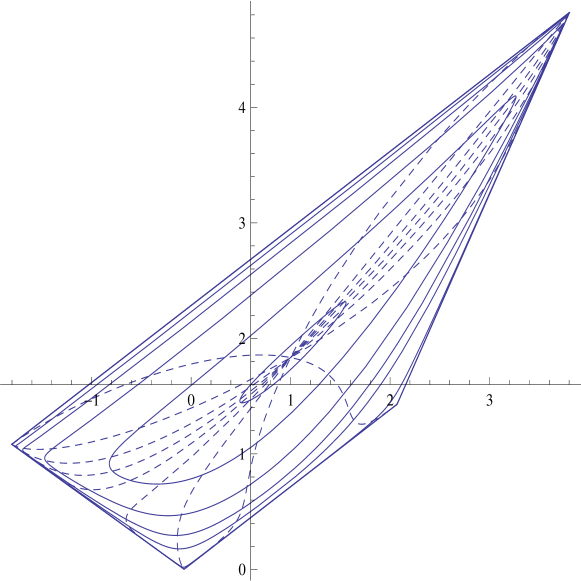
Figure 1: The curves $x({\beta},\zeta),y({\beta},\zeta)$ for fixed values of $\beta_{0}$ and variable values of $\theta$ (full lines); and for fixed values of $\theta$ and variable values of $\beta_{0}$ (dashed lines). The horizontal and the vertical axes, represent, respectively, $x({\beta},\zeta)$ and $y({\beta},\zeta)$.

Example 5.1

Let us consider the observables

$$H=\left[\begin{matrix}1&1&0&0\\ 3&1&1&0\\ 0&3&1&1\\ 0&0&3&1\end{matrix}\right],\quad K=\frac{1}{3}H^{2}.$$

and $A=H+iK.$ It may be easily seen that the numerical range of $A$ is a quadrilateral.

Let

$$x(\beta_{0},\theta)+iy(\beta_{0},\theta):={\rm Tr}\left(\frac{\mathrm{e}^{-\beta_{0}(\cos\theta H+\sin\theta K)}}{{\rm Tr}{\mathrm{e}^{-\beta_{0}(\cos\theta H+\sin\theta K)}}}(H+iK)\right),\quad x(\beta_{0},\theta),\leavevmode\nobreak\ y(\beta_{0},\theta)\in\mathbb{R}.$$

Fixing $\beta_{0}$ and varying $\theta$ we obtain a closed curve surrounding the point of maximal entropy, $1+11i/6$. Fixing $\theta$ and varying ${\beta}_{0}$, we obtain curves connecting the point $1+11i/6$ with corners of $W(H+iK)$. The full curves displayed in Figure 1 are for $\beta_{0}=0.1,0.5,1,1.5,2,4,8,16,32$ and $0<\theta<2\pi$. For $\beta_{0}=8,16,32$ the lines are not distinguishable and coincide with the boundary of $W(H+iK).$ The displayed dashed curves are for $\theta=\pi/8,\pi/4,3\pi/8,\pi/2,5\pi/8,3\pi/4,7\pi/8,\pi$ and $-32<\beta_{0}<32$. In the limit $\beta_{0}\rightarrow+\infty,$ the boundary of $W(H+iK))$ is obtained i.e., the limit of the solution $\rho_{0}$ corresponds for almost any $\theta$ to a pure state, with entropy $S=0$.

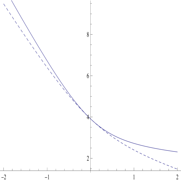
Figure 2: Illustrating the concavity of the $\log Z$ vesus $\beta$. Results obtained for $n=50.$ Hermitian case, $d=0$, full lines, and non-Hermitian case, $d=\sqrt{7}/4$, dashed lines.

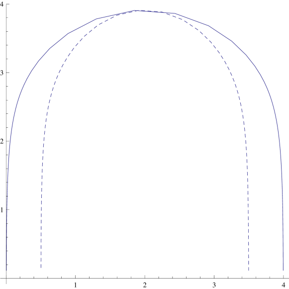
Figure 3: Illustrating the concavity of the maximum entropy vs. $\langle H\rangle$. Results obtained for $n=50.$ Hermitian case, $d=0$, full lines, and non-Hermitian case, $d=\sqrt{7}/4$, dashed lines.

Example 5.2

We consider next a model whose Hamiltonian is a Toeplitz matrix $K_{n}$, which is non-Hermitian for $d\neq 0$. To ensure the reality of the spectrum we impose the condition $|b|<1.$

$$K_{n}=\left[\begin{matrix}2&1-d&0&0&\ldots&0\\ 1+d&2&1-d&0&\ldots&0\\ 0&1+d&2&1-d&\ldots&0\\ 0&0&1+d&2&\ldots&0\\ \vdots&\vdots&\vdots&\vdots&\ddots&\vdots\\ 0&0&0&0&\ldots&2\end{matrix}\right],\leavevmode\nobreak\ \leavevmode\nobreak\ d\in\mathbb{R},\leavevmode\nobreak\ |d|<1.$$ (7)

Its eigenvalues are

$$\lambda_{k}=2-2\sqrt{1-d^{2}}\cos\frac{k\pi}{n+1}.$$

There exists $D\geq 0$ such that $DK_{n}=K_{n}^{\dagger}D.$ Figure 2 illustrates the convexity of $\log Z$ vs. $\beta$. Figure 3 illustrates the concavity of the maximum entropy vs. $\langle H\rangle$. In order to approach the partition function we use te following result on the Euler-McLaurin expansion.

Proposition 5.4

Let $n$ be a positive integer and let $f$ be a real function defined in the real interval $[0,1]$, being of class $C^{\infty}$ in $[0,1),$ $f^{\prime}(1)$ exists but $f^{\prime\prime}(1)$ does not exist. Then

$$\sum_{k=1}^{n}f\left({k\over n}\right)=n\int_{0}^{1}f(x){\rm d}x+\frac{1}{2}(f(1)-f(0))+\frac{1}{12n}(f^{\prime}(1)-f^{\prime}(0))+R_{n},$$ (8)

with

$$R_{n}=-{1\over 2n}\int_{1/n}^{1}B_{2}(\{nx\})f^{\prime\prime}(x){\rm d}x.$$ (9)

where $B_{2}(x)=x^{2}-x+1/6$ is the second Bernoulli polynomial and $\{t\}$ denotes the fractional part of $t$.

It is known that

$$\int_{0}^{n+1}\mathrm{e}^{f+h\cos(k\pi/(n+1))}{\rm d}k=\mathrm{e}^{f}(1+n)\leavevmode\nobreak\ _{0}I(h)$$

where ${}_{n}I(z)$ is the modified Bessel function of first kind.

By the Euler-MacLaurin formula, we obtain

$$\sum_{k=1}^{n}\mathrm{e}^{-\beta\lambda_{k}}$$

$$=-\mathrm{e}^{-\beta(b-\sqrt{ac})}+\sum_{k=1}^{n+1}\mathrm{e}^{-\beta\lambda_{k}}$$

$$\approx\mathrm{e}^{-\beta b}(1+n)\leavevmode\nobreak\ {{}_{0}I(\beta\sqrt{ac})}-\frac{1}{2}\left(\mathrm{e}^{-\beta(b+\sqrt{ac})}+\mathrm{e}^{-\beta(b-\sqrt{ac})}\right).$$

6 Concluding remarks

If $H$ lives in an infinite dimensional Hilbert space, different situations may occur, such as the metric operator or its inverse, or both, being, possibly, unbounded. The eigenstates of the Hamiltonian $H$ and of $H^{\dagger}$ are biorthogonal but they cannot form bases of $\cal H$ [1]. The existence of a bounded operator with bounded inverse mapping some orthonormal bases of $\cal H$ into the sets $\{\psi_{k}\}$ and $\{\widetilde{\psi}_{k}\}$ is not guaranteed, a priori. Thus, the previous procedure should be reconsidered carefully. We notice, however, that from the point of view of physics, the full Hilbert space $\cal H$ may not be needed. Nothing guarantees that all vectors in $\cal H$ have physical meaning. Let ${\cal S}:={\rm span}\{\psi_{k}\}$, ${\widetilde{\cal S}}:={\rm span}\{\widetilde{\psi}_{k}\}.$ Only vectors $\psi\in{\cal S}$ represent physical states. Although $D$ is not defined in $\cal H$, it goes from $\cal S$ to $\widetilde{\cal S}.$ The operators $H,\leavevmode\nobreak\ K,\leavevmode\nobreak\ \rho$ go from $\cal S$ to $\cal S$, the operators $H^{\dagger},\leavevmode\nobreak\ K^{\dagger},\leavevmode\nobreak\ \rho^{\dagger}$ go from $\widetilde{\cal S}$ to $\widetilde{\cal S}$. The Physical Hilbert space is the set $\cal S$ endowed with the inner product $\langle D\cdot,\cdot\rangle$ [14].

Summarizing, for $n$ finite, ${\cal H}={\cal S}=\widetilde{\cal S}.$ For $n=\infty,$ this is not so, but the proposed definitions are still meaningful.

References

• [1] F. Bagarello, J.-P. Gazeau, F.H. Szafraniec, M. Znojil, Non-Selfadjoint Operators in Quantum Physics: Mathematical Aspects, Wiley, 2015.
• [2] F. Bagarello, A concise review on pseudo-bosons, pseudo-fermions and their relatives, arXiv:1703.06730 [math-ph].
• [3] N. Bebiano, R. Lemos and J. Providência, Matrix inequalities in statistical mechanics, Linear Algebra Appl., 376 (2004), 265-273.
• [4] N. Bebiano, R. Lemos and J. Providência, Inequalities for quantum relative entropy, Linear Algebra Appl., 376 (2005), 155-172.
• [5] N. Bebiano and J. Providência, On the generalized free energy inequality, Advances in Operator Theory 2 (2017) 50-58.
• [6] N. Bebiano, J. da Providência , J. P. da Providência, Mathematical Aspects of Quantum Systems with a Pseudo-Hermitian Hamiltonian, Brazilian Journal of Physics,46 (2016) 152-156.
• [7] N. Bebiano and J. da Providência, The EMM and the Spectral Analysis of a Non Self-adjoint Hamiltonian on an Infinite Dimensional Hilbert Space, Non-Hermitian Hamiltonians in Quantum Physics. 184 Springer Proceedings in Physics, (2016)157-166
• [8] N-Bebiano and J.da Providência, Maximum entropy principle and Landau free energy inequality, Linear and Multilinear Algebra, in print.
• [9] C.M. Bender and S. Boettcher, Real Spectra in Non-Hermitian Hamiltonians Having PT Symmetry , Phys. Rev. Lett., 80 (1998) 5243-5246.
• [10] C.M. Bender, D.C. Brody and H.F. Jones, Complex Extension of Quantum Mechanics, Phys. Rev. Lett, 89 (2002) 27041.
• [11] E.T. Jaynes, Information theory and statistical mechanics, Phys. Rev. 106 (1957) 620-630; 108 (1957) 171-190.
• [12] K. R. W. Jones, Principles of quantum inference, Annals of Physics. 207 (1991) 140. Bibcode:1991AnPhy.207..140J. doi:10.1016/0003-4916(91)90182-8.
• [13] L. D. Landau and E. M. Lifshitz, Statistical Physics, Pergamon Pres, 1969.
• [14] A. Mostafazadeh, Pseudo-Hermitian Quantum Mechanics with Unbounded Metric Operators, Cite as: arXiv:1203.6241 [math-ph], Phil. Trans. R. Soc. A 371 (2013) 20120050.
• [15] A.Mostafazadeh, Exact PT-symmetry is equivalent to Hermiticity, J. Phys. A: Math. Gen. 36 (2003) 7081. Complex Extension of Quantum Mechanics, J. Math. Phys. 46 (2005) 102108;
• [16] J. da Providência, N. Bebiano and JP. da Providência, Non Hermitian operators with real spectra in Quantum Mechanics, Brazilian Journal of Physics, 41 (2011) 78-85.
• [17] F.G. Scholtz, H.B. Geyer and F.J.W. Hahne, Quasi-Hermitian operators in quantum mechanics and the variational principle, Ann. Phys. NY 213 (1992) 74.
• [18] J. von Neumann, Thermodinamik quantenmechanischer Gesamtheiten, Nachr. Ges. Wiss. Göttingen (1927) 273-291.
• [19] S. Weis, Information topologies on non-commutative state spaces, Journal of Convex Analysis, 21 (2014) 339-399.
• [20] E.H, Wichmann, Density matrices arising from incomplete measurements, J. Math. Phys., 3 (1963) 884-896.
• [21] M. Znojil, Should PT Symmetric Quantum Mechanics Be Interpreted as Nonlinear?, J. Nonlin. Math. Phys., 9 (2002) 122-123.