Deep Non-Rigid Structure from Motion
with Missing Data

Abstract

Non-Rigid Structure from Motion (NRSfM) refers to the problem of reconstructing cameras and the 3D point cloud of a non-rigid object from an ensemble of images with 2D correspondences. Current NRSfM algorithms are limited from two perspectives: (i) the number of images, and (ii) the type of shape variability they can handle. These difficulties stem from the inherent conflict between the condition of the system and the degrees of freedom needing to be modeled – which has hampered its practical utility for many applications within vision. In this paper we propose a novel hierarchical sparse coding model for NRSFM which can overcome (i) and (ii) to such an extent, that NRSFM can be applied to problems in vision previously thought too ill posed. Our approach is realized in practice as the training of an unsupervised deep neural network (DNN) auto-encoder with a unique architecture that is able to disentangle pose from 3D structure. Using modern deep learning computational platforms allows us to solve NRSfM problems at an unprecedented scale and shape complexity. Our approach has no 3D supervision, relying solely on 2D point correspondences. Further, our approach is also able to handle missing/occluded 2D points without the need for matrix completion. Extensive experiments demonstrate the impressive performance of our approach where we exhibit superior precision and robustness against all available state-of-the-art works in some instances by an order of magnitude. We further propose a new quality measure (based on the network weights) which circumvents the need for 3D ground-truth to ascertain the confidence we have in the reconstructability. We believe our work to be a significant advance over state-of-the-art in NRSFM.

1 Introduction

Building an AI capable of inferring the 3D structure and pose of an object from a single image is a problem of immense importance. Training such a system using supervised learning requires a large number of labeled images – how to obtain these labels is currently an open problem for the vision community. Rendering [1] is problematic as the synthetic images seldom match the appearance and geometry of the objects we encounter in the real-world. Hand annotation is preferable, but current strategies rely on associating the natural images with an external 3D dataset (e.g. ShapeNet [2], ModelNet [3]), which we refer to as 3D supervision. If the 3D shape dataset does not capture the variation we see in the imagery, then the problem is inherently ill-posed.

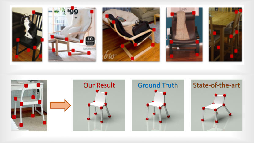
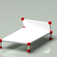
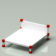
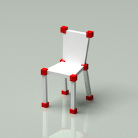
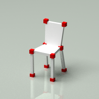
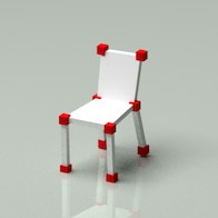
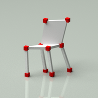
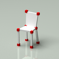
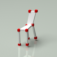
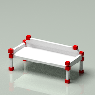
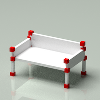
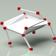
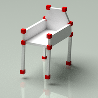
Non-Rigid Structure from Motion (NRSfM) offers computer vision a way out of this quandary – by recovering the pose and 3D structure of an object category solely from hand annotated 2D landmarks with no need of 3D supervision. Classically [4], the problem of NRSfM has been applied to objects that move non-rigidly over time such as the human body and face. Additional benchmarks have been proposed [5] for other temporally deforming non-rigid objects. But NRSfM is not restricted to non-rigid objects; it can equally be applied to rigid objects whose object categories are non-rigid [6, 7, 8]. Consider, for example, the five objects in Figure 1 (top), instances from the visual object category “chair”. Each object in isolation represents a rigid chair, but the set of all 3D shapes describing “chair” is non-rigid. In other words, each object instance can be modeled as a certain deformation from its category’s general shape.

Rigid SfM is already an ill-posed problem. It is the rigidity prior of objects that helps to obtain good results across SfM applications. NRSfM is even more challenging where rigidity is removed due to its inherent non-rigid nature. To resolve the problem of NRSfM, additional shape priors are proposed, e.g. low rank [4, 9], union-of-subspaces [10, 7], and block-sparsity [11, 6]. However, low rank is only applicable to simple non-rigid objects with limited deformations and union-of-subspaces rely heavily on frame clustering which has difficulty scaling up to large image collections. A block-sparsity prior where each shape can be represented by at most $K$ bases out of $L$, is considered as one of the most promising assumptions in terms of covering broad shape variations. This is because sparsity can be thought as a union of $\binom{L}{K}$ subspaces where $L$ could be large then an over-complete dictionary is utilized. However, pointed by our previous work [11], searching the best subspace out of $\binom{L}{K}$ is extremely hard and not robust. Based on this observation, in this paper, we propose a novel shape prior using hierarchical sparse coding. The introduced additional layers compared to single-layer sparse coding are capable of controlling the number of subspaces by learning from data such that invalid subspaces are removed while sufficient subspaces are remained for modeling shape variations. This insight is at the heart of our paper.

1.1 Contributions

We propose a novel shape prior based on hierarchical sparse coding and demonstrate that the 2D projections under weak perspective cameras can be represented by the hierarchical dictionaries in a block sparse way. Through recent theoretical innovations [12], we then show how this problem can be reinterpreted as training an unsupervised feed-forward Deep Neural Network(DNN) auto-encoder. A common drawback of DNNs when applied to reconstruction problems is that they are an opaque black-box lacking any interpretability. A strength of our approach is that the DNN is directly derived from a hierarchical block sparse dictionary learning objective – allowing for greater transparency into what the network weights are modeling. As a result we are able to formulate a measure of model quality (using the coherence of learned parameters), which helps to avoid over-fitting especially when ground-truth of training data are not available.

Our deep NRSfM is capable of handling hundreds of thousands of images and learning large parameterizations to model non-rigidity. Extensive experiments are conducted and our approach outperforms state-of-the-art methods in the order of magnitude on a number of benchmarks. Both quantitative and qualitative results demonstrate our superior performance – an example of qualitative results is shown in Figure 1.

Compared to our previous work [13], this paper offers a substantial leap forward in terms of state-of-the-art. Our approach can now handle “real-world” scenarios where camera scale and translation are unknown and there are missing or occluded 2D points. Specifically, the method is now capable of reconstructing non-rigid objects under weak perspective projection instead of orthogonal (as in [13]). Weak perspective projection is a reasonable assumption for many practical vision applications where the object’s variation in depth is small compared to their distance from the camera [14, 4, 15, 16]. Additionally, unlike our earlier work [13], this paper provides a solution to reconstruct invisible points – 2D coordinates missing due to occlusion or self-occlusion – with no need of matrix completion. These two breakthroughs make this paper substantially different from the deep NRSfM first proposed in [13] and dramatically improve its practical utilities in real-world applications.

Figure 1: In this paper, we want to reconstruct 3D shapes solely from a sequence of annotated images—shown on the top—with no need of 3D ground truth. Our proposed hierarchical sparse coding model and corresponding deep solution outperform state-of-the-arts in the order of magnitude.

1.2 Related Work

In rigid structure from motion, the rank of 3D structure is fixed, [14] since the 3D structure remains the same between frames. Based on this insight, Bregler et al. [4] advocated that non-rigid 3D structure could be represented by a linear subspace of low rank. Dai et al. [9] developed this prior further by proving that the low-rank assumption itself is sufficient to address the ill-posedness of NRSfM with no need of additional priors. They then proposed a novel algorithm based on singular value decomposition, followed by a non-linear optimization to achieve state-of-the-art performance across numerous benchmarks. The low-rank assumption has also been applied temporally [17, 18] – 3D point trajectories can be represented by pre-defined (e.g. DCT) or learned bases. Although exhibiting impressive performance, the low-rank assumption has a major drawback. The rank is strictly limited by the number of points and frames (whichever is smaller [9]). This makes low-rank NRSfM infeasible if we want to solve large-scale problems with – complex shape variations – when the number of points is substantially smaller than the number of frames.

Inspired by the intuition that complex non-rigid deformations could be clustered into a sequence of simple motions, Zhu et al. [10] proposed to model non-rigid 3D structure by a union of local subspaces. They show that clustering frames from their 2D annotations is less effective and therefore propose a novel algorithm to reconstruct 3D shapes and an estimate of the 3D-based frame affinity matrix simultaneously. The idea of union-of-subspaces was later extended to spatial-temporal domain [19] and applied to rigid object category reconstruction [7].Though the union-of-subspaces model is capable of handling complex object deformation, its holistic estimation of the entire affinity matrix – the number of frame by the number of frame matrix – impedes its scalability to large-scale problems e.g. more than tens of thousand frames.

Inspired by the union-of-subspaces assumption, a block-sparsity prior [11, 20, 6] was proposed as a more generic and elegant prior for NRSfM. The sparsity prior can be viewed as being mathematically equivalent to the union of all possible local subspaces. This is advantageous as it circumvents the need for a messy affinity matrix – since all local subspaces are being considered. Further, since the method is entertaining many local subspaces it is also able to model much more complex 3D shapes than single subspace low-rank methods. However, the sheer number of subspaces that can be entertained by the block-sparsity prior is its fundamental drawback. Since there are so many possible subspaces to choose from, the approach is quite sensitive to noise dramatically limiting its applicability to “real-world” NRSfM problems. In this paper we want to leverage the elegance and expressibility of the block-sparsity prior without suffering from its inherent sensitivity to noise.

Drover et al. [21] recently applied neural networks for NRSfM in an unsupervised manner. Drover et al. used a GAN to generate potential 3D structures and ensure their consistency across novel viewpoints through the GAN’s discriminator. Although intriguing, this approach to date has only been shown effective for 3D human skeletons – whereas our approach exhibits state-of-the-art performance across multiple disparate object classes. Further, unlike [21], the connection of our approach to sparse dictionary learning facilitates a measure (based on dictionary coherence) of the uniqueness of the 3D reconstruction without having any 3D ground-truth. Finally, it is unclear how Drover et al. handles missing points – again limiting the applicability of their approach to to “real-world” problems.

Missing correspondences are inevitable when annotating objects because key points are often occluded by other objects or itself, shown in Figure 1 (top). This requires any practical NRSfM algorithm to be tolerant to missing 2D points. Two solutions are usually utilized: (i) a mask is introduced indicating the visibility of 2D points to the objective function [22, 23, 6], or (ii) the employment of a matrix completion algorithm to recover the missing 2D points a priori from which then the NRSfM algorithm [9, 24, 25] is applied. In this paper, we follow the former strategy and show how this is implemented by a feed-forward neural network.

1.3 Background

Sparse dictionary learning can be considered as an unsupervised learning task and divided into two sub-problems: (i) dictionary learning, and (ii) sparse code recovery. Let us consider sparse code recovery problem, where we estimate a sparse representation $\mathbf{z}$ for a measurement vector $\mathbf{x}$ given the dictionary $\mathbf{D}$, i.e.

$$\min_{\mathbf{z}}\|\mathbf{x}-\mathbf{D}\mathbf{z}\|_{2}^{2}\quad\ \mathrm{s.t.}\ \|\mathbf{z}\|_{0}<\lambda,$$ (1)

where $\lambda$ related to the trust region controls the sparsity of recovered code. One classical algorithm to recover the sparse representation is Iterative Shrinkage and Thresholding Algorithm (ISTA) [26, 27, 28]. ISTA iteratively executes the following two steps with $\mathbf{z}^{[0]}=\mathbf{0}$:

$$\mathbf{v}=\mathbf{z}^{[i]}-\alpha\mathbf{D}^{T}(\mathbf{D}\mathbf{z}^{[i]}-\mathbf{x}),$$ (2)

$$\mathbf{z}^{[i+1]}=\operatorname*{argmin}_{\mathbf{u}}\frac{1}{2}\|\mathbf{u}-\mathbf{v}\|^{2}_{2}+\tau\|\mathbf{u}\|_{1},$$ (3)

which first uses the gradient of $\|\mathbf{x}-\mathbf{D}\mathbf{z}\|_{2}^{2}$ to update $\mathbf{z}^{[i]}$ in step size $\alpha$ and then finds the closest sparse solution using an $\ell_{1}$ convex relaxation. It can be demonstrated that the second step has a closed-form solution that is

$$\mathbf{z}^{[i+1]}=\eta(\mathbf{v};\tau).$$ (4)

where $\eta$ represents a element-wise soft-thresholding operation, formally defined as

$$\eta(x;b)=\begin{cases}x-b&\text{if}~{}x>b,\\ x+b&\text{if}~{}x<-b,\\ 0&\text{otherwise}.\end{cases}$$ (5)

Therefore, ISTA can be summarized as the following recursive equation:

$$\mathbf{z}^{[i+1]}=\eta\big{(}\mathbf{z}^{[i]}-\alpha\mathbf{D}^{T}(\mathbf{D}\mathbf{z}^{[i]}-\mathbf{x});\tau\big{)},$$ (6)

where $\tau$ is related to $\lambda$ for controlling sparsity.

Recently, Papyan [12] proposed to use ISTA and sparse coding to reinterpret feed-forward neural networks. They argue that feed-forward passing a single-layer neural network $\mathbf{z}=\eta(\mathbf{D}^{T}\mathbf{x};b)$ can be considered as one iteration of ISTA in (6) when setting $\alpha=1$ and $\tau=b$. Based on this insight, the authors extend this interpretation to feed-forward neural network with $N$ layers

$$\mathbf{z}_{1} =\eta(\mathbf{D}_{1}^{T}\mathbf{x};b_{1})$$ (7)

$$\mathbf{z}_{2} =\eta(\mathbf{D}_{2}^{T}\mathbf{z}_{1};b_{2})$$

$$\quad\vdots$$

$$\mathbf{z}_{N} =\eta(\mathbf{D}_{N}^{T}\mathbf{z}_{N-1};b_{N})$$

as executing a sequence of single-iteration ISTA, serving as an approximate solution to the hierarchical sparse coding problem: find $\{\mathbf{z}_{i}\}_{i=1}^{N}$, such that

$$\mathbf{x}=\mathbf{D}_{1}\mathbf{z}_{1} ,\quad\|\mathbf{z}_{1}\|_{0}<\lambda_{1},$$ (8)

$$\mathbf{z}_{1}=\mathbf{D}_{2}\mathbf{z}_{2} ,\quad\|\mathbf{z}_{2}\|_{0}<\lambda_{2},$$

$$\vdots ,\quad\quad\vdots$$

$$\mathbf{z}_{N-1}=\mathbf{D}_{N}\mathbf{z}_{N} ,\quad\|\mathbf{z}_{N}\|_{0}<\lambda_{N},$$

where the bias terms $\{b_{i}\}_{i=1}^{N}$ (in a similar manner to $\tau$) are related to $\{\lambda_{i}\}_{i=1}^{N}$, adjusting the sparsity of recovered code. Furthermore, they reinterpret back-propagating through the deep neural network as learning the dictionaries $\{\mathbf{D}_{i}\}_{i=1}^{N}$. This connection offers a novel reinterpretation of DNNs through the lens of hierarchical sparse dictionary learning. In this paper, we extend this reinterpretation to the block sparse scenario and apply it to solving our NRSfM problem.

2 Problem Formulation

In the context of NRSfM, the weak perspective projection model is a reasonable assumption since the many of objects we deal with in vision applications have a much smaller depth variation compared to their distance from the camera. We shall start from the orthogonal projection model in this section and then generalize to weak perspective projection in Section 5. Under orthogonal projection, NRSfM deals with the problem of factorizing a 2D projection matrix $\mathbf{W}\in\mathbb{R}^{P\times 2}$, given $P$ points, as the product of a 3D shape matrix $\mathbf{S}\in\mathbb{R}^{P\times 3}$ and a camera matrix $\mathbf{M}\in\mathbb{R}^{3\times 2}$. Formally,

$$\mathbf{W}=\mathbf{S}\mathbf{M},$$ (9)

$$\mathbf{W}=\begin{bmatrix}u_{1}&v_{1}\\ u_{2}&v_{2}\\ \vdots&\vdots\\ u_{P}&v_{P}\end{bmatrix},~{}\mathbf{S}=\begin{bmatrix}x_{1}&y_{1}&z_{1}\\ x_{2}&y_{2}&z_{2}\\ \vdots&\vdots&\vdots\\ x_{P}&y_{P}&z_{P}\end{bmatrix},~{}\mathbf{M}^{T}\mathbf{M}=\mathbf{I}_{2},$$ (10)

where $(u_{i},v_{i})$ and $(x_{i},y_{i},z_{i})$ are the image and world coordinates of the $i$-th point respectively. The goal of NRSfM is to recover simultaneously the shape $\mathbf{S}$ and the camera $\mathbf{M}$ for each projection $\mathbf{W}$ in a given set $\mathbb{W}$ of 2D landmarks. In a general NRSfM including SfC, this set $\mathbb{W}$ could contain deformations of a non-rigid object or various instances from an object category.

3 Modeling via hierarchical sparse coding

Kong et al. [11] argued that an effective solution for NRSfM can be found by assuming the vectorization of $\mathbf{S}$ can be represented by a dictionary sparsely:

$$\mathbf{s}=\mathbf{D}\boldsymbol{\psi},\quad\|\boldsymbol{\psi}\|_{0}<\lambda\;\;.$$ (11)

This paper introduces additional layers and therefore a hierarchical sparse model is proposed:

$$\mathbf{s}=\mathbf{D}_{1}\boldsymbol{\psi}_{1} ,\quad\|\boldsymbol{\psi}_{1}\|_{0}<\lambda_{1},$$ (12)

$$\boldsymbol{\psi}_{1}=\mathbf{D}_{2}\boldsymbol{\psi}_{2} ,\quad\|\boldsymbol{\psi}_{2}\|_{0}<\lambda_{2},$$

$$\vdots ,\quad\quad\vdots$$

$$\boldsymbol{\psi}_{N-1}=\mathbf{D}_{N}\boldsymbol{\psi}_{N} ,\quad\|\boldsymbol{\psi}_{N}\|_{0}<\lambda_{N},$$

where $\mathbf{D}_{1}\in\mathbb{R}^{3P\times K_{1}},\mathbf{D}_{2}\in\mathbb{R}^{K_{1}\times K_{2}},\dots,\mathbf{D}_{N}\in\mathbb{R}^{K_{N-1}\times K_{N}}$ are hierarchical dictionaries and $\boldsymbol{\psi}_{1}\in\mathbb{R}^{K_{1}}$, $\boldsymbol{\psi}_{2}\in\mathbb{R}^{K_{2}}$, $\dots$, $\boldsymbol{\psi}_{N}\in\mathbb{R}^{K_{N}}$ are hierarchical sparse codes. In this prior, each non-rigid shape is represented by a sequence of dictionaries and corresponding non-negative sparse codes hierarchically. Each sparse code is determined by its lower-level neighbor and affects the next-level. The additional layers introduced by this hierarchy increase the number of variables, and thus increase the degree of freedom of the system. However, these additional layers actually result in a more constrained and thus stable sparse code recovery process.

Sparse code recovery algorithms in general attempt to solve two problems: 1) select the best subspace and 2) estimate the closest representation within the subspace. These two problems could be solved simultaneously or alternatively, but the quality of recovered sparse code highly relies on the former. If the desired subspace is given from oracle, then the sparse coding problem degenerates to a linear system. However, without knowing the size of the desired subspace, the number of valid subspaces in (11) is combinatorial to the number of dictionary atoms $K$ i.e. $\sum_{n=1}^{K}\binom{K}{n}$. Selecting the best subspace out of such large number of candidates is considerably difficult, especially when using over-complete dictionaries. This reveals the conflict between the quality of sparse code recovery and the representing capacity of the dictionary, and further explains the sensitivity of [11] to non-compressible sequences.

The additional layers introduced in this paper alleviate the dilemma. In (12), the sparse code $\boldsymbol{\psi}_{1}$ is not completely free but represented by the subsequent dictionaries. Therefore, the number of subspaces is not combinatorial to $K_{1}$ but controlled by the subsequent dictionaries $\{\mathbf{D}_{i}\}_{i=2}^{N}$. If the subsequent dictionaries are learned properly, they could serve as a filter so that only functional subspaces remain and redundant ones are removed. This directly breaks the combinatorial explosion of the number of subspaces and consequently maintains the robustness of sparse code recovery. Based on this observation, we are able to utilize substantially over-complete dictionaries to model a highly deformable object from a large scale image collection with no worries about reconstructability and robustness.

3.1 Hierarchical Block Sparse Coding

Given the proposed hierarchical sparse coding model, shown in (12), we now build a conduit from the 2D correspondences $\mathbf{W}$ to the proposed shape code $\{\boldsymbol{\psi}_{i}\}_{i=1}^{k}$. Since $\mathbf{s}\in\mathbb{R}^{3P}$ in (12) is the vectorization of $\mathbf{S}\in\mathbb{R}^{P\times 3}$, it can be well modeled via i.e. $\mathbf{S}=\mathbf{D}^{\sharp}_{1}(\boldsymbol{\psi}_{1}\otimes\mathbf{I}_{3})$ where $\otimes$ is the Kronecker product and $\mathbf{D}_{1}^{\sharp}\in\mathbb{R}^{P\times 3K_{1}}$ is a reshape of $\mathbf{D}_{1}\in\mathbb{R}^{3P\times K_{1}}$ [9]. It is known that $\mathbf{A}\mathbf{B}\otimes\mathbf{I}=(\mathbf{A}\otimes\mathbf{I})(\mathbf{B}\otimes\mathbf{I})$ given two matrices $\mathbf{A},\mathbf{B}$, and identity matrix $\mathbf{I}$. Based on this lemma, we can derive that

$$\mathbf{S}=\mathbf{D}^{\sharp}_{1}(\boldsymbol{\psi}_{1}\otimes\mathbf{I}_{3}) ,\quad\|\boldsymbol{\psi}_{1}\|_{0}<\lambda_{1},$$ (13)

$$\boldsymbol{\psi}_{1}\otimes\mathbf{I}_{3}=(\mathbf{D}_{2}\otimes\mathbf{I}_{3})(\boldsymbol{\psi}_{2}\otimes\mathbf{I}_{3}) ,\quad\|\boldsymbol{\psi}_{2}\|_{0}<\lambda_{2},$$

$$\vdots ,\quad\quad\vdots$$

$$\boldsymbol{\psi}_{N-1}\otimes\mathbf{I}_{3}=(\mathbf{D}_{N}\otimes\mathbf{I}_{3})(\boldsymbol{\psi}_{N}\otimes\mathbf{I}_{3}) ,\quad\|\boldsymbol{\psi}_{N}\|_{0}<\lambda_{N}.$$

Further, from (9), by right multiplying the camera matrix $\mathbf{M}\in\mathbb{R}^{3\times 2}$ to the both sides of (13) and denote $\boldsymbol{\Psi}_{i}=\boldsymbol{\psi}_{i}\otimes\mathbf{M}$, we obtain that

$$\mathbf{W}=\mathbf{D}^{\sharp}_{1}\boldsymbol{\Psi}_{1} ,\quad\|\boldsymbol{\Psi}_{1}\|_{0}^{(3\times 2)}<\lambda_{1},$$ (14)

$$\boldsymbol{\Psi}_{1}=(\mathbf{D}_{2}\otimes\mathbf{I}_{3})\boldsymbol{\Psi}_{2} ,\quad\|\boldsymbol{\Psi}_{2}\|_{0}^{(3\times 2)}<\lambda_{2},$$

$$\vdots ,\quad\quad\vdots$$

$$\boldsymbol{\Psi}_{N-1}=(\mathbf{D}_{N}\otimes\mathbf{I}_{3})\boldsymbol{\Psi}_{N} ,\quad\|\boldsymbol{\Psi}_{N}\|_{0}^{(3\times 2)}<\lambda_{N},$$

where $\|\cdot\|_{0}^{(3\times 2)}$ divides the argument matrix into blocks with size $3\times 2$ and counts the number of active blocks. Since $\boldsymbol{\psi}_{i}$ has active elements less than $\lambda_{i}$, $\boldsymbol{\Psi}_{i}$ has active blocks less than $\lambda_{i}$, that is $\boldsymbol{\Psi}_{i}$ is block sparse. This derivation demonstrates that if the shape vector $\mathbf{s}$ satisfies the hierarchical sparse coding prior described by (12), then its 2D projection $\mathbf{W}$ must be in the format of hierarchical block sparse coding described by (14). We hereby interpret NRSfM as a hierarchical block sparse dictionary learning problem, i.e. factorizing $\mathbf{W}$ as products of hierarchical dictionaries $\{\mathbf{D}_{i}\}_{i=1}^{N}$ and block sparse coefficients $\{\boldsymbol{\Psi}_{i}\}_{i=1}^{N}$.

4 Deep Neural Network Solution

Figure 2: Architecture of our proposed deep NRSfM. The network can be divided into 1) Encoder: from 2D correspondences $\mathbf{W}$ to the hidden block sparse code $\boldsymbol{\Psi}_{N}$, 2) Bottleneck: from hidden block sparse code $\boldsymbol{\Psi}_{N}$ to hidden regular sparse code $\boldsymbol{\psi}_{N}$ and camera, 3) Decoder: from hidden regular sparse code $\boldsymbol{\psi}_{N}$ to 3D reconstructed shape $\mathbf{S}$. The encoder and decoder are intentionally designed to share convolution kernels (i.e. dictionaries) and form a symmetric formulation. The symbol $a\times b,c\to d$ refers to the convolution layer using kernel size $a\times b$ with $c$ input channels and $d$ output channels.

Before solving the hierarchical block sparse coding problem in (14), we first consider a single-layer problem:

$$\min_{\mathbf{Z}}\|\mathbf{X}-\mathbf{D}\mathbf{Z}\|_{F}^{2}\quad\ \mathrm{s.t.}\ ~{}\|\mathbf{Z}\|_{0}^{(3\times 2)}<\lambda.$$ (15)

Inspired by ISTA, we propose to solve this problem by iteratively executing the following two steps:

$$\mathbf{V}=\mathbf{Z}^{[i]}-\alpha\mathbf{D}^{T}(\mathbf{D}\mathbf{Z}^{[i]}-\mathbf{X}),$$ (16)

$$\mathbf{Z}^{[i+1]}=\operatorname*{argmin}_{\mathbf{U}}\frac{1}{2}\|\mathbf{U}-\mathbf{V}\|^{2}_{F}+\tau\|\mathbf{U}\|_{F1}^{(3\times 2)},$$ (17)

where $\|\cdot\|_{F1}^{(3\times 2)}$ is defined as the summation of the Frobenius norm of each $3\times 2$ block, serving as a convex relaxation of the block sparsity constraint. Recall the regular sparse situation in Section 1.3. Analogous to (4), we use an approximate solution to (17) for computational efficiency, i.e.

$$\mathbf{Z}^{[i+1]}=\eta(\mathbf{V};\mathbf{b}\otimes\mathbf{1}_{3\times 2}),$$ (18)

where $\eta$ represents a element-wise soft-thresholding operation defined in (5), $\mathbf{1}_{3\times 2}$ denotes a 3-by-2 matrix filled with one and $\mathbf{b}$ is a vector that controls the trust region for each block. Based on this approximation, a single-iteration block ISTA with step size $\alpha=1$ can be represented by :

$$\mathbf{Z}=\eta(\mathbf{D}^{T}\mathbf{X};\mathbf{b}\otimes\mathbf{1}_{3\times 2}),$$ (19)

4.1 Encoder

Recall from Section 1.3 that the feed-forward pass through a deep neural network can be considered as a sequence of single ISTA iterations and thus provides an approximate recovery of hierarchical sparse codes. We follow the same scheme – sequentially using single-iteration block ISTA – to solve the hierarchical block sparse coding problem (14) i.e.

$$\boldsymbol{\Psi}_{1} =\eta((\mathbf{D}^{\sharp}_{1})^{T}\mathbf{W};\mathbf{b}_{1}\otimes\mathbf{1}_{3\times 2}),$$ (20)

$$\boldsymbol{\Psi}_{2} =\eta((\mathbf{D}_{2}\otimes\mathbf{I}_{3})^{T}\boldsymbol{\Psi}_{1};\mathbf{b}_{2}\otimes\mathbf{1}_{3\times 2}),$$

$$\quad\vdots$$

$$\boldsymbol{\Psi}_{N} =\eta((\mathbf{D}_{N}\otimes\mathbf{I}_{3})^{T}\boldsymbol{\Psi}_{N-1};\mathbf{b}_{N}\otimes\mathbf{1}_{3\times 2}),$$

where $\{\mathbf{b}_{i}\}_{i=1}^{N}$ are learnable parameters, controlling the block sparsity. This formula composes the encoder of our proposed deep neural network.

It is worth mentioning that setting $\{\mathbf{b}_{i}\}_{i=1}^{N}$ as learnable parameters is crucial because in previous NRSfM algorithms – low-rank [9], union-of-subspaces [10], or block-sparsity [11] priors – the weight associated with shape regularization (e.g.low-rank or sparsity) is determined through a cumbersome and slow grid-search process. In our approach, this weighting is learned simultaneously with all other parameters, removing the need for irksome cross-validation.

4.2 Code and Camera Recovery

Recall that in Section 3.1, we define $\boldsymbol{\Psi}=\boldsymbol{\psi}\otimes\mathbf{M}$. By denoting the $k$-th block in $\boldsymbol{\Psi}_{N}$ as $\boldsymbol{\Psi}_{N}^{k}$ and the $k$-th element in $\boldsymbol{\psi}_{N}$ as $\boldsymbol{\psi}_{N}^{k}$. we have

$$\boldsymbol{\Psi}_{N}^{k}=\boldsymbol{\psi}_{N}^{k}\mathbf{M}.$$ (21)

Now, we want to estimate the regular sparse hidden code $\boldsymbol{\psi}_{N}$ and camera $\mathbf{M}$ given $\boldsymbol{\Psi}_{N}$. It is obvious that if one of them is known beforehand, then the other one can be solved easily. For example, if $\mathbf{M}$ is known, then $\boldsymbol{\psi}_{N}^{k}$ can be estimated by

$$\boldsymbol{\psi}_{N}^{k}=\frac{1}{6}\sum_{i=1}^{3}\sum_{j=1}^{2}\frac{[\boldsymbol{\Psi}_{N}^{k}]_{ij}}{[\mathbf{M}]_{ij}}=\sum_{i=1}^{3}\sum_{j=1}^{2}\frac{1}{6[\mathbf{M}]_{ij}}[\boldsymbol{\Psi}_{N}^{k}]_{ij},$$ (22)

where $[\cdot]_{ij}$ denotes the $ij$-th element in the argument matrix. Note that actually a single element in camera M and its correspondence in $\boldsymbol{\Psi}_{N}$ are sufficient to estimate the scaler $\boldsymbol{\psi}_{N}^{k}$, but, for robust estimation, an average over all elements ($3\times 2$ block results in totally 6 elements) is utilized here. Further, if $\boldsymbol{\psi}_{N}$ is known, then $\mathbf{M}$ can be estimated by

$$\mathbf{M}=\frac{1}{K_{N}}\sum_{k=1}^{K_{N}}\frac{\boldsymbol{\Psi}_{N}^{k}}{\boldsymbol{\psi}_{N}^{k}}=\sum_{k=1}^{K_{N}}\frac{1}{K_{N}\boldsymbol{\psi}_{N}^{k}}\boldsymbol{\Psi}_{N}^{k}.$$ (23)

Note that a single element in $\boldsymbol{\psi}_{N}$ and a corresponding block in $\boldsymbol{\Psi}_{N}$ is again sufficient to estimate $\mathbf{M}$ but, for robustness, we utilize an average across all blocks.

In the literature of the field [9, 29, 11], these two coupled variables are mainly solved by a carefully designed algorithm that utilizes the orthonormal constraint to solve the camera first and then the sparse hidden code. However, this heuristic is quite fragile and it is even worse when the estimation of $\boldsymbol{\Psi}_{N}$ is bothered by noise. Further, it has difficulty deciding the sign ambiguity of each sparse code. In this paper, we propose a novel relaxation, decoupling equations (22) and (23) by introducing two learnable parameters $\beta$ and $\gamma$, specifically,

$$\boldsymbol{\psi}_{N}^{k}=\sum_{i=1}^{3}\sum_{j=1}^{2}\beta_{ij}[\boldsymbol{\Psi}_{N}^{k}]_{ij},$$ (24)

$$\mathbf{M}=\sum_{k=1}^{K_{N}}\gamma_{k}\boldsymbol{\Psi}_{N}^{k}.$$ (25)

It is clear that $\boldsymbol{\psi}$ and $\mathbf{M}$ are intrinsically linked – but our proposed approach seems to ignore this dependency. We resolve this inconsistency, however, by enforcing an orthonormal constraint for the camera in our loss function shown in Section 4.4. This relaxation has the further advantage of eliminating fragile heuristics and giving substantial computational savings. Figure 2 represents this process via convolutions for conciseness and descent visualization.

4.3 Decoder

Given the sparse hidden code $\boldsymbol{\psi}_{N}$ and hierarchical dictionaries $\{\mathbf{D}_{i}\}_{i=1}^{N}$, the 3D shape vector $\mathbf{s}$ could be recovered via (12). In practice, instead of forming a purely linear decoder, we preserve soft-thresholding in each layer. This non-linear decoder is expected to further enforce sparsity and improve robustness. Formally,

$$\boldsymbol{\psi}_{N-1} =\eta(\mathbf{D}_{N}\boldsymbol{\psi}_{N};\mathbf{b}_{N}^{\prime}),$$ (26)

$$\quad\vdots$$

$$\boldsymbol{\psi}_{1} =\eta(\mathbf{D}_{2}\boldsymbol{\psi}_{2};\mathbf{b}_{2}^{\prime}),$$

$$\mathbf{s} =\mathbf{D}^{\sharp}_{1}\boldsymbol{\psi}_{1}.$$

This portion forms the decoder of our deep neural network.

4.4 Loss Function

Until now, the 3D shape $\mathbf{S}$ is estimated via the proposed encoder and decoder architecture given the hierarchical dictionaries, which is denoted as $\mathcal{S}\big{(}\mathbf{W}|\{\mathbf{D}_{i}\}_{i=1}^{N}\big{)}$ for simplicity. Further, the camera $\mathbf{M}$ is also estimated via the encoder and a linear combination given the dictionaries, which is denoted as $\mathcal{M}\big{(}\mathbf{W}|\{\mathbf{D}_{i}\}_{i=1}^{N}\big{)}$. Our loss function is thus defined as

$$\min_{\{\mathbf{D}\}_{i=1}^{N}} \sum_{\mathbf{W}\in\mathbb{W}}\left\|\mathbf{W}-\mathcal{S}\big{(}\mathbf{W}|\{\mathbf{D}_{i}\}_{i=1}^{N}\big{)}\mathbf{U}\mathbf{V}^{T}\right\|_{F}$$ (27)

$$\ \mathrm{s.t.} \mathbf{U}\Sigma\mathbf{V}^{T}=\mathcal{M}\big{(}\mathbf{W}|\{\mathbf{D}_{i}\}_{i=1}^{N}\big{)},$$

which is the summation of reprojection error. To ensure the success of the orthonormal constraint on the camera, we introduce the Singular Value Decomposition (SVD) to hard code the singular value of $\mathbf{M}$ to be exact ones. As mentioned in Section 4.2, reprojecting the estimated 3D shape via the estimated camera (i.e. left multiplying $\mathbf{M}$ to $\mathbf{S}$) implicitly re-build the bonds between the camera $\mathbf{M}$ and the sparse hidden code $\boldsymbol{\psi}_{N}$ (in the form of 3D shape $\mathbf{S}$).

4.5 Implementation Issues

The Kronecker product of identity matrix $\mathbf{I}_{3}$ dramatically increases the time and space complexity of our approach. To eliminate it and make parameter sharing easier in modern deep-learning environments (e.g. TensorFlow, PyTorch), we reshape the filters and features so that the matrix multiplication in each step can be equivalently computed via multi-channel convolution ($*$) and transposed convolution ($*^{T}$). We first reshape the 2D input correspondences $\mathbf{W}$ into a three-dimensional tensor $\mathsf{w}\in\mathbb{R}^{1\times 2\times P}$, which can be considered in the deep-learning community as a $1\times 2$ image with $P$ channels. Then, we reshape the first dictionary $\mathbf{D}_{1}^{\sharp}$ into a four-dimensional tensor $\mathsf{d}_{1}^{\sharp}\in\mathbb{R}^{3\times 1\times K_{1}\times P}$, which can be interpreted as a convolutional kernel in size $3\times 1$ with $K_{1}$ input channels and $P$ output channels. Therefore, we have

$$(\mathbf{D}_{1}^{\sharp})^{T}\mathbf{W}=\mathsf{d}_{1}^{\sharp}*^{T}\mathsf{w},$$ (28)

which helps us to maintain a uniform dictionary shape and is consequently easier to share parameters. We then reshape each dictionary $\mathbf{D}_{i}$ other than the first one into a four-dimensional tensor $\mathsf{d}_{i}\in\mathbb{R}^{1\times 1\times K_{i}\times K_{i-1}}$ and the hidden block sparse code $\boldsymbol{\Psi}_{i}$ into a three-dimensional tensor $\Psi_{i}\in\mathbb{R}^{3\times 2\times K_{i}}$. Therefore, we have

$$(\mathbf{D}_{i+1}\otimes\mathbf{I}_{3})^{T}\boldsymbol{\Psi}_{i}=\mathsf{d}_{i+1}*^{T}\Psi_{i},$$ (29)

which helps us to eliminate the Kronecker product. Finally, based on the above reshape, the dictionary-code multiplication is simplified as

$$\mathbf{D}_{i}\boldsymbol{\psi}_{i}=\mathsf{d}_{i}*\psi_{i}.$$ (30)

As for the architecture design, we only control three hyper parameters: 1) the number of dictionaries $N$, 2) the number of atoms in the first dictionary $K_{1}$, and 3) the number of atoms in the last dictionary $K_{N}$. We then linearly sample $K_{2},\dots,K_{N-1}$ between $K_{1}$ and $K_{N}$. As for training, we implement our neural network via TensorFlow and train it using an Adam optimizer with a learning rate exponentially decayed from 0.001.

4.6 Replacing Soft-thresholding via ReLU

Recall in Section 1.3, Papyan et al. replaced the soft-thresholding operator $\eta$ by ReLU as a result of the non-negativity constraint. Actually, it can easily be demonstrated that a linear (block) sparse model can always be transferred equivalently to a model only using non-negative (block) sparse code i.e.

$$\mathbf{W}=\mathbf{D}\boldsymbol{\Psi}=\begin{bmatrix}\mathbf{D}&-\mathbf{D}\end{bmatrix}\begin{bmatrix}\boldsymbol{\Psi}^{+}\\ -\boldsymbol{\Psi}^{-}\end{bmatrix}.$$ (31)

where $\boldsymbol{\Psi}^{+}$ and $\boldsymbol{\Psi}^{-}$ are positive and negative parts of $\boldsymbol{\Psi}$ respectively and $\boldsymbol{\Psi}^{+}+\boldsymbol{\Psi}^{-}=\boldsymbol{\Psi}$. The concatenation of $\boldsymbol{\Psi}^{+}$ and $-\boldsymbol{\Psi}^{-}$ is still block sparse and now becomes non-negative. From this observation, we introduce the non-negativity constraints without the loss of generality and relax the dictionaries so that they are not bothered by mirrored structures. Interestingly, our proposed method on estimating cameras in (25) is compatible with the change, i.e.

$$\mathbf{M}=\sum_{k=1}^{K_{N}}\gamma_{k}\boldsymbol{\Psi}_{N}^{k}=\sum_{k=1}^{K_{N}}\gamma_{k}(\boldsymbol{\Psi}_{N}^{k})^{+}\sum_{k=1}^{K_{N}}-\gamma_{k}(-\boldsymbol{\Psi}_{N}^{k})^{-}.$$ (32)

All of these enable us to utilize ReLU to replace the soft-thresholding. ReLU is good because it is closer to deep learning packages while soft-thresholding is more compact in size of parameters. An experiment comparing between soft-thresholding and ReLU is in the Appendix. It is demonstrated that no discernible difference in the accuracy of reconstructions is observed. Therefore, we decide to use ReLU for the remaining sections and experiments, making our approach closer to leading techniques in deep learning and more accessible and approachable to the public.

5 Occlusion and Weak Perspective

5.1 Occlusion

It is commonly observed in real images that a certain portion of key points are occluded by other objects or the object itself. For example, we typically see two wheels of a sedan instead of four. An often-used strategy is to recover the missing entries in $\mathbf{W}$ by matrix completion before feeding it into the proposed pipeline. A commonly used shape prior for matrix completion is low-rank, even for some union-of-subspaces algorithms [7]. This is problematic.

In this paper, we derive a solution from the ISTA to handle missing entries, which turns out as a quite simple but well-functioning operation. We observe that missing entries break the first layer of encoder but once $\boldsymbol{\Psi}_{1}$ is estimated, all other layers can execute with no trouble. Based on this observation, we first introduce a diagonal matrix $\boldsymbol{\Omega}\in\mathbb{R}^{P\times P}$, whose element on the main diagonal is zero if the corresponding point in $\mathbf{W}$ is missing; otherwise, one and all other elements except diagonal are zeros. With the help of the mask $\boldsymbol{\Omega}$, the objective function w.r.t the first layer is

$$\min_{\boldsymbol{\Psi}_{1}}\|\boldsymbol{\Omega}(\mathbf{W}-\mathbf{D}_{1}^{\sharp}\boldsymbol{\Psi}_{1})\|_{F}^{2}\quad\text{s.t.}~{}\|\boldsymbol{\Psi}_{1}\|_{0}^{(3\times 2)}<\lambda_{1}.$$ (33)

Following the same derivation in Section 4, a masked ISTA is to iteratively execute the following two steps:

$$\mathbf{V}=\boldsymbol{\Psi}_{1}^{[i]}-\alpha(\mathbf{D}_{1}^{\sharp})^{T}\boldsymbol{\Omega}^{T}\boldsymbol{\Omega}(\mathbf{D}_{1}^{\sharp}\boldsymbol{\Psi}_{1}^{[i]}-\mathbf{W}),$$ (34)

$$\boldsymbol{\Psi}_{1}^{[i+1]}=\operatorname*{argmin}_{\mathbf{U}}\frac{1}{2}\|\mathbf{U}-\mathbf{V}\|^{2}_{F}+\tau\|\mathbf{U}\|_{F1}^{(3\times 2)},$$ (35)

By (18), it is implied that the single-iteration block ISTA with mask is

$$\boldsymbol{\Psi}_{1}=\eta\big{(}(\mathbf{D}_{1}^{\sharp})^{T}\boldsymbol{\Omega}\mathbf{W}-\mathbf{b}\otimes\mathbf{I}_{3\times 2}\big{)}.$$ (36)

This is equivalently to set missing entries to zero and then feed into the proposed deep neural network.

5.2 Scale and Translation

The main difference between weak perspective and orthogonal projection is additional scale and translation besides rotation. Due to the ambiguity between camera scale and 3D shape size, we do not solve the camera scale explicitly, but consider the scale to be one and reconstruct a scaled 3D shape. To alleviate the effect of the scale on optimization, we normalize the 2D correspondences into a unit bounding box before feeding into the proposed neural network.

Translation is not a problem and can even be eliminated when all points are visible. This is because one can always remove the camera translation by shifting the center of 2D correspondences to the image origin. However, this is not true when some correspondences are missing. Formally, $i\in\Omega$ denotes that the $i$-th point is visible and $(u_{i},v_{i})$ is the image coordinate of the $i$-th point. Shifting the center of all points (where missing entries are set to zero) to the origin remains a translation residual

$$\frac{1}{n}\sum_{i}\begin{bmatrix}u_{i}\\ v_{i}\end{bmatrix}-\frac{1}{n}\sum_{i\in\Omega}\begin{bmatrix}u_{i}\\ v_{i}\end{bmatrix}=\frac{1}{n}\sum_{i\not\in\Omega}\begin{bmatrix}u_{i}\\ v_{i}\end{bmatrix}.$$ (37)

When key points distribute closely in a cluster and a small portion of them are missing, the residual translation could be treated as some sort of noise perturbation and consequently need no further operation. Otherwise, we need to solve the translation explicitly.

Consider the camera projection with translation $\mathbf{t}$, i.e.

$$\mathbf{W}=\begin{bmatrix}u_{1}&v_{1}\\ u_{2}&v_{2}\\ \vdots&\vdots\\ u_{P}&v_{P}\end{bmatrix}=\begin{bmatrix}x_{1}&y_{1}&z_{1}&1\\ x_{2}&y_{2}&z_{2}&1\\ \vdots&\vdots&\vdots&\vdots\\ x_{P}&y_{P}&z_{P}&1\end{bmatrix}\begin{bmatrix}\mathbf{M}\\ \mathbf{t}^{T}\end{bmatrix}.$$ (38)

We could introduce an auxiliary variable $\epsilon$

$$\mathbf{W}=\begin{bmatrix}x_{1}&y_{1}&z_{1}&\epsilon\\ x_{2}&y_{2}&z_{2}&\epsilon\\ \vdots&\vdots&\vdots&\vdots\\ x_{P}&y_{P}&z_{P}&\epsilon\end{bmatrix}\begin{bmatrix}\mathbf{M}\\ \mathbf{t}^{T}/\epsilon\end{bmatrix}=\tilde{\mathbf{S}}\tilde{\mathbf{M}}$$ (39)

such that $\tilde{\mathbf{S}}$ satisfies the proposed hierarchical sparse model in (13) after appending ones to each dictionary. Therefore, a similar neural network could be derived from a 4-by-2 block sparse ISTA as $\tilde{\mathbf{M}}\in\mathbb{R}^{4\times 2}$.

Figure 3: Qualitative evaluation on IKEA dataset. From top to bottom are tables, chairs, sofas and tables. From left to right are ground-truth and respectively reconstructions by ours, RIKS [25], KSTA [22], NLO [23], SFC [6], CNS [24], BMM [9]. In each rendering, red cubes are reconstructed points but the planes and bars are manually added for descent visualization.

6 Experiments

We conduct extensive experiments to evaluate the performance of our deep solution to solving NRSfM and SfC problems. For quantitative evaluation, we follow the metric normalized mean 3D error reported in [30, 9, 22, 7]. Our implementation, processed data, and pre-trained models are publicly accessible for future comparison.

6.1 IKEA Furniture

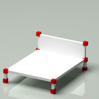
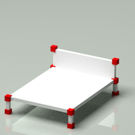
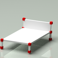
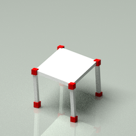
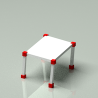
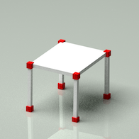
We first apply our method to a furniture dataset, IKEA dataset [31, 32]. The IKEA dataset contains four object categories: bed, chair, sofa, and table. For each object category, we project the 3D ground-truth by the orthogonal cameras annotated from real images. Since fully annotated images are limited, we thereby augment them with 2,000 projections under randomly generated orthogonal cameras. The errors are evaluated only on frames using cameras from real images. Numbers are summarized into Table I. One can observe that our method outperforms baselines in the order of magnitude, clearly showing the superiority of our model. For qualitative evaluation, we randomly select a frame from each object category and show these frames in Figure 3 against ground-truth and baselines. As shown, our reconstructed landmarks effectively depict the 3D geometry of objects and our method is able to cover subtle geometric details.

TABLE I: Quantitative Comparison against State-Of-The-Art Algorithms using IKEA Dataset in Normalized 3D Error.

Furnitures	Bed	Chair	Sofa	Table	Average	Relative
KSTA [22]	0.069	0.158	0.066	0.217	0.128	12.19
BMM [9]	0.059	0.330	0.245	0.211	0.211	20.12
CNR [24]	0.227	0.163	0.835	0.186	0.352	33.55
NLO [23]	0.245	0.339	0.158	0.275	0.243	23.18
RIKS [25]	0.202	0.135	0.048	0.218	0.117	11.13
SPS [11]	0.971	0.946	0.955	0.280	0.788	74.96
SFC [6]	0.247	0.195	0.233	0.193	0.217	20.67
OURS	0.004	0.019	0.005	0.012	0.010	1.00

6.2 PASCAL3D+ Dataset

We then apply our method to the PASCAL3D+ dataset [16], which contains twelve object categories. Following the experiment setting reported in [7], we also utilize eight categories: aeroplane, bicycle, bus, car, chair, dining table, motorbike and sofa. To explore the performance in various situations, we design experiments with respect to

• Orthogonal or weak perspective projection?

• Complete or missing measurement?

• Clean data or Gaussian noise perturbed?

Totally, there are eight configurations. Specifically, for projection setting, we randomly generate rotation matrices for orthogonal projection while additionally utilizing random scale and random translation for weak perspective projection. For missing data, we randomly sample approximately $10\%$ of points missing for each category. For noise, we corrupt 2D correspondences with a zero mean Gaussian perturbation, following the same noise ratio in [7]. For the translation residual, we simply treat it as noise and handle it with a 3-by-2 block sparse model. In Table II, we report the normalized mean 3D error of our proposed method and state-of-the-arts: KSTA [22], RIKS [25], CNS [24], NLO [23], SFC [6], SPS [11], and BMM [9]. For readers’ interest, one can compare our numbers against the Table 2 in [7] for more baselines.

TABLE II: Quantitative Comparison against State-Of-The-Art Algorithms using PASCAL3D Dataset. In each configuration, numbers from top to bottom are for category aeroplane, bicycle, bus, car, chair, diningtable motorbike and sofa.

		No Noise Perturbation								Added Noise Perturbation
		OURS	KSTA	RIKS	CNS	NLO	SFC	SPS	BMM	OURS	KSTA	RIKS	CNS	NLO	SFC	SPS	BMM
Orthogonal Projection	Complete Measurement	0.013	0.161	0.562	0.636	0.175	0.499	0.902	1.030	0.026	0.175	0.583	0.626	0.167	0.518	0.761	1.177
		0.003	0.249	0.826	0.732	0.285	0.370	0.959	1.247	0.009	0.253	0.779	0.715	0.916	0.367	1.065	1.424
		0.004	0.201	0.578	0.443	0.262	0.255	0.902	0.728	0.012	0.196	0.450	0.442	0.320	0.253	1.096	0.754
		0.003	0.124	0.497	0.497	0.135	0.284	0.955	1.006	0.012	0.162	0.557	0.496	0.192	0.285	0.879	0.915
		0.009	0.191	0.748	0.540	0.145	0.223	1.018	1.381	0.028	0.190	0.668	0.554	0.107	0.224	0.927	1.251
		0.030	0.244	0.778	0.549	0.234	0.220	0.707	1.351	0.040	0.238	0.721	0.521	0.450	0.219	0.968	1.420
		0.001	0.254	0.703	0.647	0.320	0.356	1.090	1.033	0.004	0.251	0.722	0.629	0.168	0.366	0.938	1.029
		0.007	0.401	0.798	0.623	0.055	0.302	0.779	1.017	0.020	0.333	0.725	0.627	0.064	0.297	1.041	1.315
	Missing Measurement	0.033	0.533	0.515	0.693	0.348	0.496	1.076	1.154	0.065	0.434	0.514	0.707	0.382	0.493	0.815	1.199
		0.021	0.584	0.540	0.854	0.106	0.376	1.112	1.372	0.028	0.566	0.560	0.835	0.459	0.372	1.201	1.286
		0.018	0.357	0.316	0.517	0.317	0.254	1.273	0.728	0.057	0.364	0.323	0.526	0.079	0.245	0.791	0.743
		0.010	0.400	0.334	0.598	0.089	0.286	0.918	1.014	0.023	0.391	0.299	0.587	0.111	0.285	1.077	1.244
		0.024	0.599	0.581	0.601	0.102	0.228	1.184	1.242	0.066	0.571	0.479	0.593	0.103	0.229	1.153	1.274
		0.040	0.554	0.473	0.602	0.171	0.224	1.264	1.414	0.050	0.494	0.408	0.587	0.177	0.228	1.019	1.098
		0.009	0.539	0.501	0.729	0.177	0.366	0.892	1.117	0.032	0.523	0.528	0.730	0.154	0.363	1.100	1.157
		0.015	0.573	0.567	0.728	0.911	0.301	1.214	1.171	0.039	0.576	0.590	0.727	0.080	0.307	1.252	1.017
Weak Perspective Projection	Complete Measurement	0.034	0.402	0.460	0.667	0.192	0.500	1.123	1.055	0.046	0.525	0.489	0.644	0.206	0.527	0.961	1.203
		0.008	0.576	0.817	0.707	0.595	0.373	1.172	1.301	0.029	0.618	0.729	0.760	0.930	0.368	1.202	1.331
		0.017	0.480	0.582	0.458	0.205	0.251	1.380	0.743	0.044	0.384	0.443	0.443	0.666	0.248	0.820	0.739
		0.015	0.369	0.573	0.504	0.175	0.284	1.090	1.051	0.022	0.409	0.475	0.524	0.178	0.285	0.836	1.342
		0.013	0.621	0.832	0.540	0.197	0.224	0.970	1.220	0.026	0.497	0.622	0.543	0.122	0.226	1.283	1.284
		0.025	0.647	0.829	0.533	0.428	0.220	0.927	1.447	0.068	0.585	0.629	0.506	0.303	0.220	0.993	1.123
		0.003	0.614	0.739	0.662	0.180	0.359	1.406	1.069	0.018	0.607	0.789	0.671	0.159	0.362	1.101	1.019
		0.022	0.609	0.792	0.632	0.070	0.295	0.976	0.980	0.041	0.606	0.684	0.644	0.062	0.301	1.603	1.165
	Missing Measurement	0.102	0.461	0.531	0.727	0.670	0.502	1.162	1.150	0.157	0.449	0.571	0.737	0.742	0.493	0.984	1.220
		0.048	0.499	0.572	0.875	0.115	0.372	1.312	1.279	0.084	0.668	0.708	0.895	0.141	0.375	1.003	1.405
		0.066	0.356	0.341	0.553	0.091	0.250	0.912	0.752	0.091	0.383	0.365	0.557	0.139	0.253	0.985	0.752
		0.027	0.402	0.403	0.637	0.093	0.280	0.949	0.954	0.081	0.355	0.358	0.619	0.109	0.293	1.023	1.063
		0.077	0.484	0.485	0.607	0.118	0.227	1.107	1.263	0.122	0.522	0.434	0.601	0.123	0.224	1.037	1.263
		0.091	0.463	0.465	0.594	0.174	0.232	1.210	1.229	0.136	0.558	0.528	0.612	0.173	0.225	1.151	1.510
		0.056	0.561	0.656	0.779	0.201	0.367	1.119	1.125	0.051	0.544	0.585	0.763	0.191	0.369	1.039	1.017
		0.066	0.529	0.615	0.728	0.081	0.311	1.730	1.150	0.082	0.543	0.548	0.730	0.156	0.299	0.890	1.146

From Table II, one can observe that our proposed method achieves considerably more accurate reconstructions for all cases, and for some cases, more than ten times the amount of smaller 3D errors than state-of-the-arts. It clearly demonstrates the high precision of our proposed deep neural network. By comparing between clean and noisy configurations, it is shown that our proposed method has high robustness, where our method applied on noisy data even outperforms state-of-the-arts on clean data. By comparing between orthogonal and weak perspective projections, it is demonstrated that our proposed 3-by-2 block sparse model can handle scale and translation properly, even with missing data. In the configuration with missing measurement, KSTA, RIKS, BMM, CNS, and SPS use the matrix completion algorithm proposed by [33] to recover missing entries first, but our proposed method, SFC, and NLO can directly optimize over partially-visible 2D measurements, which are more capable at handling missing data. This is verified by Table II, where OURS, SFC, and NLO sacrifice less performance than others when handling missing data. For qualitative evaluation, we use “motorbike” as an exemplar category and randomly select a frame from four configurations: 1) orthogonal+complete+noise, 2) orthogonal+missing+noise, 3) weak perspective+complete+noise, and 4) weak perspective+missing+noise, showing in Figure 4. One can observe that our proposed method outperforms KSTA, RIKS, CNS and SPS obviously and beat NLO and SFC in reconstruction details, e.g. handlebar. The figure also verifies that KSTA, RIKS, CNS, and SPS break easily with missing points while ours, SFC, and NLO maintain a nice stability against missing entries.

Figure 4: Qualitative evaluation on PASCAL3D dataset. From top to bottom are configurations 1) orthogonal projection with no missing points, 2) orthogonal projection with missing points, 3) weak perspective projection with no missing points, 4) weak perspective projection with missing points. All these four configurations are perturbed by Gaussian noise. From left to right are ground-truth, ours, KSTA [22], RIKS [25], CNS [24], NLO [23], SFC [6], SPS [11]. In each rendering of reconstruction, red cubes are reconstructed points but the planes and bars are manually added for visualization.

TABLE III: Quantitative Comparison aginst State-Of-The-Arts using CMU Motion Capture Dataset in Normalized 3D Error

SUBJECT	OURS	CNS	NLO	SPS	UNSEEN
1	0.176	0.613	1.218	1.282	0.362
5	0.221	0.657	1.160	1.122	0.331
18	0.082	0.542	0.917	0.954	0.438
23	0.054	0.604	0.999	0.880	0.388
64	0.082	0.543	1.219	1.120	0.174
70	0.040	0.473	0.837	1.010	0.090
102	0.116	0.582	1.145	1.079	0.413
106	0.114	0.637	1.016	0.958	0.195
123	0.041	0.479	1.009	0.828	0.092
127	0.095	0.645	1.051	1.022	0.389

6.3 Large-Scale NRSfM on CMU Motion Capture

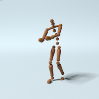
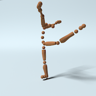
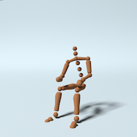
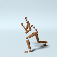
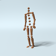
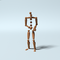
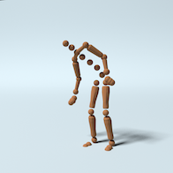
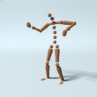
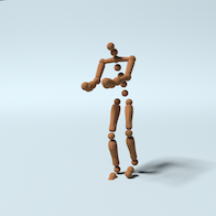
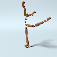
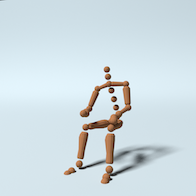
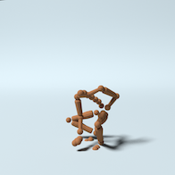
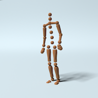
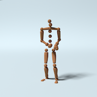
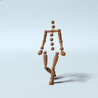
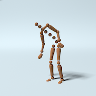
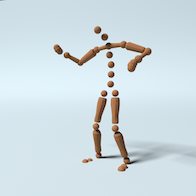
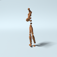
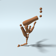
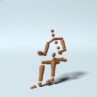
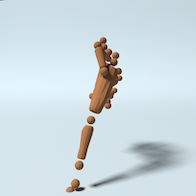
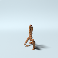
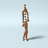
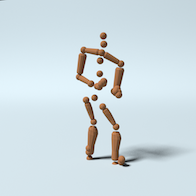
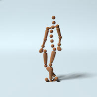
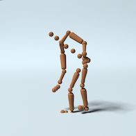
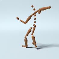
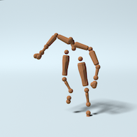
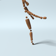
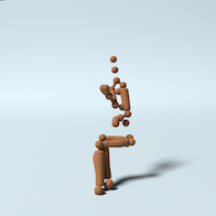
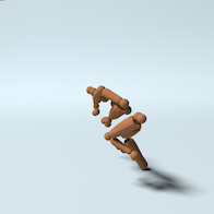
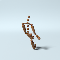
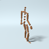
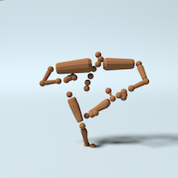
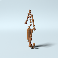
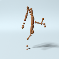
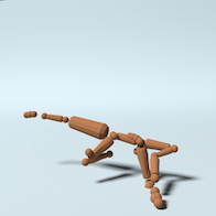
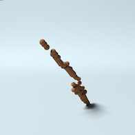
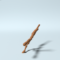
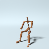
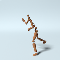
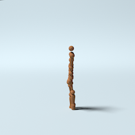
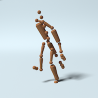
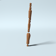
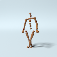
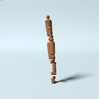
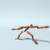
To evaluate the performance of our method on a large scale image sequence, we apply our method to solving the problem of NRSfM, using the CMU motion capture dataset. We randomly select 10 subjects out of 144, and for each subject, we concatenate $80\%$ of motions to form large image collections and leave the remaining $20\%$ as unseen motions for testing generalization. In this experiment, each subject contains more than ten thousand frames under randomly generated orthogonal projections. We compare our method against state-of-the-art methods, summarized in Table III. Due to the huge volume of frames, KSTA [22], BMM [9], MUS [7], RIKS [25], and SFC [6] all fail and thus are omitted in the table. We also report the normalized mean 3D error on unseen motions, labeled as UNSEEN. From Table III, one can see that our method obtains impressive reconstruction performance and outperforms all others again in every sequence. Moreover, our network generalizes well with unseen data, which implies the potential utility of our model to the application of single image 3D reconstruction. For qualitative evaluation, we randomly select a frame from each subject and render the reconstructed human skeleton in Figure 7, which visually verifies the impressive performance of our deep solution.

Figure 5: Normalized mean 3D error on CMU Motion Capture dataset with Gaussian noise perturbation. The blue solid line is ours while the red dashed line is CNS [24], the lowest error of state-of-the-arts with no noise perturbation.

6.3.1 Robustness analysis

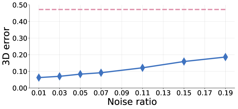
To analyze the robustness of our method, we retrain the neural network for Subject 70, using projected points perturbed by Gaussian noise. The results are summarized in Figure 5. The noise ratio is defined as $\|\text{noise}\|_{F}/\|\mathbf{W}\|_{F}$. One can see that the error increases slowly while adding a higher magnitude of noise; when adding up to $20\%$ noise to image coordinates, our method in blue still achieves better reconstruction compared to the best baseline with no noise perturbation (in red). This experiment clearly demonstrates the robustness of our model and its high accuracy against state-of-the-art works.

6.3.2 Explicitly solve translation

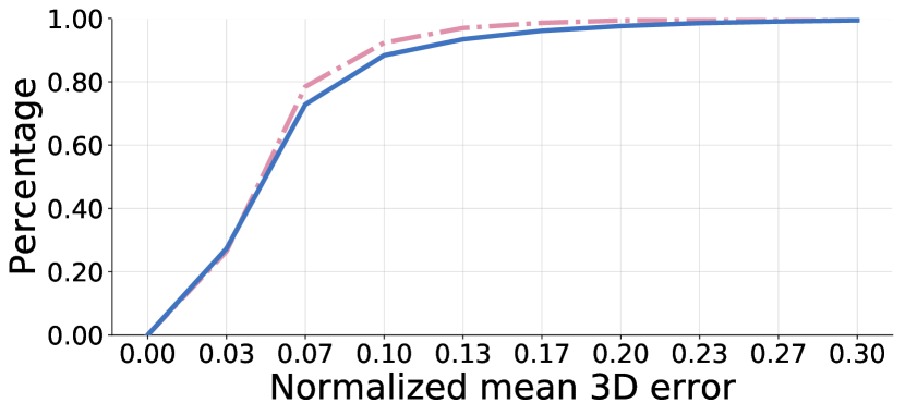
In this experiment, we verify the performance of the proposed 4-by-2 block sparse model. We focus on Subject 23, following the same experiment setting as above, except adding randomly generated translation. To avoid removing translation, we do not normalize 2D correspondences. We then apply the proposed 4-by-2 block sparse model to the data with translation and compare it to the 3-by-2 block sparse model without translation. The normalized mean 3D error of the 4-by-2 model is 0.060, which is very close to the error without translation, i.e. 0.054, and lower than state-of-the-arts without translation in the order of magnitude, as shown in Table III. To give a clearer sense of the quality of the reconstructed 3D shape, we draw two cumulative error plots in Figure 6 that show the percentage of frames below a certain normalized mean 3D error. The two plots are mostly identical, implying the success of our 4-by-2 model.

Figure 6: Percentage below a certain normalized mean 3D error. The blue solid line is our 4-by-2 block sparse model, proposed to solve translation explicitly. The red dashed line is our 3-by-2 block sparse model, applied on zero-centered data. These two plots are mostly identical.

Figure 7: Qualitative evaluation on CMU Motion Capture dataset. From top to bottom are ground-truth, and respectively reconstructions by ours, CNS [24], SPS [11], NLO [23]. From left to right are a randomly sampled frame from subjects 1, 5, 18, 23, 64, 70, 102, 106, 123, 127. In each rendering, spheres are reconstructed landmarks but bars are for descent visualization. In each reconstruction, 3D shapes are alighted to the ground-truth by a orthonormal matrix.

Figure 8: Normalized mean 3D error v.s. maximum possible number of missing points. Maximum possible number of missing points equals to three denotes every frame has to have one, two, or three missing points. The blue bar is our proposed network. The red bar is the best baseline when all points are visible, i.e. CNS in Table III.

6.3.3 Missing points

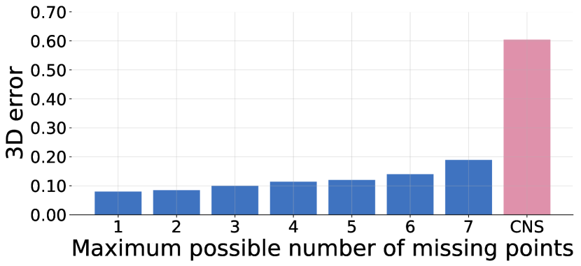
In this experiment, we explore the capability of handling missing data. We focus on Subject 23 under orthogonal projection and sequentially train and test our proposed network on data with a different percentage of missing points. Specifically, we control the maximum possible number of missing points and evaluate the performance from one to seven out of 31 total points. For example, when the maximum possible number of missing points is three, then each frame has to have one, two, or three missing points in uniform distribution. We visualize the normalized mean 3D error in each case in Figure 8 and append the lowest error achieved by state-of-the-arts under the complete measurement assumption as a baseline. One can see that the 3D error increases when the maximum possible number of missing points grows. However, even making approximately 20% (7/31) of points invisible, our proposed method still outperforms the best baseline with no missing points, i.e. CNS 0.604 in Table III.

6.3.4 Coherence as guide

Over-fitting is commonly observed in the deep learning community, especially in the NRSfM area, where over-fitting to 2D correspondences will dramatically hurt the quality of reconstructions. To solve this problem, we borrow a tool from compressed sensing – mutual coherence [34]. Mutual coherence measures the similarity between atoms in a dictionary. It is often used to depict the dictionary quality and build the bounds of sparse code reconstructability. During training for each subject, we compute the normalized mean 3D error and the coherence of the last dictionary in a fixed training iteration interval. By drawing the scatter plot of the error and the coherence, we observe a strong correlation, shown in Figure 9. This implies that the coherence of the final dictionary could be used as a measure of model quality.

Figure 9: A scatter plot of the normalized mean 3D error v.s. the coherence of the final dictionary. The blue line is fitted based on the red points. Shading presents the quality of linear regression. From left to right are, respectively, for Subjects 5, 18, and 64.

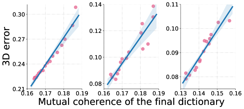
Recall the proposed block sparse model in (14), wherein every block sparse code $\boldsymbol{\Psi}_{i}$ is constrained by its subsequent representation and thus, the quality of code recovery depends not only on the quality of the corresponding dictionary but also the subsequent layers. However, this is not applicable to the final code $\boldsymbol{\Psi}_{N}$, making it overly reliant upon the final dictionary $\mathbf{D}_{N}$. From this perspective, the quality of the final dictionary measured by mutual coherence could serve as a lower bound of the entire system. With the help of the coherence, we could avoid over-fitting even when 3D evaluation is not available. This improves the utility of our deep NRSfM in applications without 3D ground-truth.

Figure 10: Qualitative evaluation on real images with hand-annotated 2D correspondences. Some images have missing points, due to occlusion. From top to bottom are aeroplanes, bicycles, chairs, and dining tables. For each pair, the left is an image with key points in red and the right is our reconstruction. In each rendering of reconstruction, red cubes are reconstructed points, but the planes and bars are manually added for descent visualization. Our method successfully captures shape variations presented in the images, e.g. table width-length ratio, the position of aeroplane wings, bicycle handlebar, and so forth.

6.4 Real Images

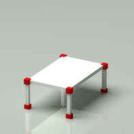
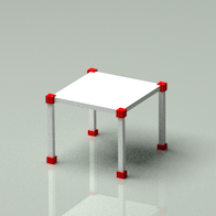
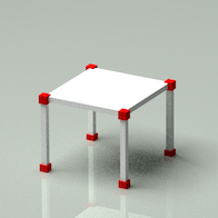
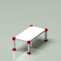
Our proposed network is designed for applications on large-scale image sequences of highly deformable objects, especially object categories. However, to our best knowledge, commonly-used object datasets mostly contain less than one hundred images of reasonable quality, a number which is greatly insufficient to train a neural network. For example, most objects in the PASCAL3D dataset have more than 50% occluded points. To demonstrate the performance of our proposed network, we apply the model pre-trained on synthetic images to real images with hand annotated correspondences. Due to the absence of 3D ground-truth, we qualitatively evaluate the reconstructed shapes and show them in Figure 10. One can see that our proposed neural network successfully reconstructs the 3D shape for each image and impressively captures the subtle shape variation presented in the image, e.g. the table width-length ratio, the position of aeroplane wings, the bicycle handlebar and so forth.

7 Discussion

This paper utilizes the weak-perspective projection to approximate the perspective projection. Though still not perspective, the jump from orthogonal projection (used in our previous work [13]) to weak-perspective allows us to apply our proposed neural network to practical scenarios, e.g. real images with hand-annotated landmarks. This feasibility is substantially a larger improvement than increasing accuracy via the perspective projection. As for the future research, we believe, rather than our used feed-forward network, a recurrent network could be more appropriate to handle the non-linearity of the perspective projection. Moreover, a recurrent network could also provides a better chance to handle a large portion of missing points. We believe, it is also promising to apply the basic ideas of this paper to the dual space, trajectory reconstruction. Due to the continuity of object trajectory, introducing convolution to the hierarchical sparse model is an interesting attempt.

8 Conclusion

In this paper, we proposed to use the hierarchical sparse coding as a novel prior assumption for representing 3D non-rigid shapes and designed an innovative encoder-decoder neural network to solve the problem of NRSfM. The proposed deep neural network was derived by generalizing the classical sparse coding algorithm, ISTA, to a block sparse scenario. The proposed network architecture is mathematically interpretable as a hierarchical block sparse dictionary learning solver. Extensive experiments demonstrated our superior performance against the state-of-the-art methods on various configurations including orthogonal projections, weak perspective projection, noise perturbations, missing points, real images, and even unseen shape variations. Finally, we propose to use the coherence of the final dictionary as a generalization measure, offering a practical way to avoid over-fitting and select the best model without 3D ground-truth.

Chen Kong is currently working toward the PhD degree at the Robotics Institute at Carnegie Mellon University. He received his Bechelor’s degree from Tsinghua University, Beijing, China, in 2014. His research interests include computer vision and machine learning, especially non-rigid structure from motion and model-based object 3D reconstruction. He is a student member of the IEEE.

Simon Lucey received the PhD degree from the Queensland University of Technology, Brisbane, Australia, in 2003. He is an Associate Research Professor at the Robotics Institute at Carnegie Mellon University. He also holds an adjunct professorial position at the Queensland University of Technology. His research interests include computer vision and machine learning, and their application to human behavior. He is a member of the IEEE.

References

- [1] H. Su, C. R. Qi, Y. Li, and L. J. Guibas, “Render for cnn: Viewpoint estimation in images using cnns trained with rendered 3d model views,” in Proceedings of the IEEE International Conference on Computer Vision, 2015, pp. 2686–2694.
- [2] A. X. Chang, T. A. Funkhouser, L. J. Guibas, P. Hanrahan, Q. Huang, Z. Li, S. Savarese, M. Savva, S. Song, H. Su, J. Xiao, L. Yi, and F. Yu, “Shapenet: An information-rich 3d model repository,” CoRR, vol. abs/1512.03012, 2015. [Online]. Available: http://arxiv.org/abs/1512.03012
- [3] Z. Wu, S. Song, A. Khosla, F. Yu, L. Zhang, X. Tang, and J. Xiao, “3d shapenets: A deep representation for volumetric shapes,” in Proceedings of the IEEE conference on computer vision and pattern recognition, 2015, pp. 1912–1920.
- [4] C. Bregler, A. Hertzmann, and H. Biermann, “Recovering non-rigid 3d shape from image streams,” in Computer Vision and Pattern Recognition, 2000. Proceedings. IEEE Conference on, vol. 2. IEEE, 2000, pp. 690–696.
- [5] S. H. N. Jensen, A. Del Bue, M. E. B. Doest, and H. Aanæs, “A benchmark and evaluation of non-rigid structure from motion,” arXiv preprint arXiv:1801.08388, 2018.
- [6] C. Kong, R. Zhu, H. Kiani, and S. Lucey, “Structure from category: a generic and prior-less approach,” International Conference on 3DVision (3DV), 2016.
- [7] A. Agudo, M. Pijoan, and F. Moreno-Noguer, “Image collection pop-up: 3d reconstruction and clustering of rigid and non-rigid categories,” in Proceedings of the IEEE Conference on Computer Vision and Pattern Recognition, 2018, pp. 2607–2615.
- [8] S. Vicente, J. Carreira, L. Agapito, and J. Batista, “Reconstructing pascal voc,” in 2014 IEEE Conference on Computer Vision and Pattern Recognition. IEEE, 2014, pp. 41–48.
- [9] Y. Dai, H. Li, and M. He, “A simple prior-free method for non-rigid structure-from-motion factorization,” International Journal of Computer Vision, vol. 107, no. 2, pp. 101–122, 2014.
- [10] Y. Zhu, D. Huang, F. D. L. Torre, and S. Lucey, “Complex non-rigid motion 3d reconstruction by union of subspaces,” in Computer Vision and Pattern Recognition (CVPR), 2014 IEEE Conference on. IEEE, 2014, pp. 1542–1549.
- [11] C. Kong and S. Lucey, “Prior-less compressible structure from motion,” Computer Vision and Pattern Recognition (CVPR), 2016.
- [12] V. Papyan, Y. Romano, and M. Elad, “Convolutional neural networks analyzed via convolutional sparse coding,” The Journal of Machine Learning Research, vol. 18, no. 1, pp. 2887–2938, 2017.
- [13] C. Kong and S. Lucey, “Deep interpretable non-rigid structure from motion,” arXiv preprint arXiv:1902.10840, 2019.
- [14] C. Tomasi and T. Kanade, “Shape and motion from image streams under orthography: a factorization method,” International Journal of Computer Vision, vol. 9, no. 2, pp. 137–154, 1992.
- [15] J. Xiao, J. Chai, and T. Kanade, “A closed-form solution to non-rigid shape and motion recovery,” International Journal of Computer Vision, vol. 67, no. 2, pp. 233–246, 2006.
- [16] Y. Xiang, R. Mottaghi, and S. Savarese, “Beyond pascal: A benchmark for 3d object detection in the wild,” in IEEE Winter Conference on Applications of Computer Vision. IEEE, 2014, pp. 75–82.
- [17] I. Akhter, Y. Sheikh, and S. Khan, “In defense of orthonormality constraints for nonrigid structure from motion,” in Computer Vision and Pattern Recognition, 2009. CVPR 2009. IEEE Conference on. IEEE, 2009, pp. 1534–1541.
- [18] K. Fragkiadaki, M. Salas, P. Arbelaez, and J. Malik, “Grouping-based low-rank trajectory completion and 3d reconstruction,” in Advances in Neural Information Processing Systems, 2014, pp. 55–63.
- [19] A. Agudo and F. Moreno-Noguer, “Dust: Dual union of spatio-temporal subspaces for monocular multiple object 3d reconstruction,” in Proceedings of the IEEE Conference on Computer Vision and Pattern Recognition, 2017, pp. 6262–6270.
- [20] X. Zhou, M. Zhu, S. Leonardos, K. Derpanis, and K. Daniilidis, “Sparseness meets deepness: 3d human pose estimation from monocular video,” arXiv preprint arXiv:1511.09439, 2015.
- [21] D. Drover, R. MV, C.-H. Chen, A. Agrawal, A. Tyagi, and C. Phuoc Huynh, “Can 3d pose be learned from 2d projections alone?” in Proceedings of the European Conference on Computer Vision (ECCV), 2018, pp. 0–0.
- [22] P. F. Gotardo and A. M. Martinez, “Kernel non-rigid structure from motion,” in Computer Vision (ICCV), 2011 IEEE International Conference on. IEEE, 2011, pp. 802–809.
- [23] A. Del Bue, F. Smeraldi, and L. Agapito, “Non-rigid structure from motion using ranklet-based tracking and non-linear optimization,” Image and Vision Computing, vol. 25, no. 3, pp. 297–310, 2007.
- [24] M. Lee, J. Cho, and S. Oh, “Consensus of non-rigid reconstructions,” in Proceedings of the IEEE Conference on Computer Vision and Pattern Recognition, 2016, pp. 4670–4678.
- [25] O. C. Hamsici, P. F. Gotardo, and A. M. Martinez, “Learning spatially-smooth mappings in non-rigid structure from motion,” in European Conference on Computer Vision. Springer, 2012, pp. 260–273.
- [26] I. Daubechies, M. Defrise, and C. De Mol, “An iterative thresholding algorithm for linear inverse problems with a sparsity constraint,” Communications on Pure and Applied Mathematics: A Journal Issued by the Courant Institute of Mathematical Sciences, vol. 57, no. 11, pp. 1413–1457, 2004.
- [27] C. J. Rozell, D. H. Johnson, R. G. Baraniuk, and B. A. Olshausen, “Sparse coding via thresholding and local competition in neural circuits,” Neural computation, vol. 20, no. 10, pp. 2526–2563, 2008.
- [28] A. Beck and M. Teboulle, “A fast iterative shrinkage-thresholding algorithm with application to wavelet-based image deblurring,” in Acoustics, Speech and Signal Processing, 2009. ICASSP 2009. IEEE International Conference on. IEEE, 2009, pp. 693–696.
- [29] I. Akhter, Y. Sheikh, S. Khan, and T. Kanade, “Trajectory space: A dual representation for nonrigid structure from motion,” IEEE Transactions on Pattern Analysis and Machine Intelligence, vol. 33, no. 7, pp. 1442–1456, 2011.
- [30] ——, “Nonrigid structure from motion in trajectory space,” in Advances in neural information processing systems, 2009, pp. 41–48.
- [31] J. J. Lim, H. Pirsiavash, and A. Torralba, “Parsing IKEA Objects: Fine Pose Estimation,” ICCV, 2013.
- [32] J. Wu, T. Xue, J. J. Lim, Y. Tian, J. B. Tenenbaum, A. Torralba, and W. T. Freeman, “Single image 3d interpreter network,” European Conference on Computer Vision (ECCV), 2016.
- [33] P. F. Gotardo and A. M. Martinez, “Computing smooth time trajectories for camera and deformable shape in structure from motion with occlusion,” Pattern Analysis and Machine Intelligence, IEEE Transactions on, vol. 33, no. 10, pp. 2051–2065, 2011.
- [34] D. L. Donoho, M. Elad, and V. N. Temlyakov, “Stable recovery of sparse overcomplete representations in the presence of noise,” IEEE Transactions on information theory, vol. 52, no. 1, pp. 6–18, 2006.
![[Uncaptioned image]](/html/1907.13123/assets/jpg/chenk.jpg) |