Piggyback search for fast radio bursts using Nanshan 26m and Kunming 40m radio telescopes – I. Observing and data analysis systems, discovery of a mysterious peryton

Abstract

We present our piggyback search for fast radio bursts using the Nanshan 26m Radio Telescope and the Kunming 40m Radio Telescope. The observations are performed in the L-band from 1380 MHz to 1700 MHz at Nanshan and S-band from 2170 MHz to 2310 MHz at Kunming. We built the Roach2-based FFT spectrometer and developed the real-time transient search software. We introduce a new radio interference mitigation technique named zero-DM matched filter and give the formula of the signal-to-noise ratio loss in the transient search. Though we have no positive detection of bursts in about 1600 and 2400 hours data at Nanshan and Kunming respectively, an intriguing peryton was detected at Nanshan, from which hundreds of bursts were recorded. Perytons are terrestrial radio signals that mimic celestial fast radio bursts. They were first reported at Parkes and identified as microwave oven interferences later. The bursts detected at Nanshan show similar frequency swept emission and have double-peaked profiles. They appeared in different sky regions in about tens of minutes observations and the dispersion measure index is not exactly 2, which indicates the terrestrial origin. The peryton differs drastically from the known perytons detected at Parkes, because it appeared in a precise period of $p=1.71287\pm 0.00004$ s. Its origin remains unknown.

1 Introduction

Lorimer et al. (2007) discovered the first fast radio burst (FRB). At first, it was unclear whether this was a new type of celestial radio source, or radio frequency interference (RFI). Particularly, FRBs share two major similarities with the ground-based RFI: 1) both have very bright flux ($\sim$0.3 Jy to $\sim$100 Jy); 2) both have durations of a few milliseconds. Furthermore, since the Lorimer burst was not observed again in the follow-up observations, it was impossible to assert the source origin.

On the other hand, Lorimer burst may well be celestial. The burst signal showed a characteristic cold plasma dispersion relation, that the group delay at frequency $\nu$ is

$$t=4.149\,{\rm DM}\left(\nu_{\rm 1,GHz}^{-2}-\nu_{\rm 2,GHz}^{-2}\right)\,{\rm ms}\,.$$ (1)

The dispersion measure, DM, is the column density of free electrons in the unit of pc cm^-3 along the line of sight, i.e. ${\rm DM}\equiv\int{n_{\mathrm{e}}dl}$ where $n_{\rm e}$ is the electron density. Due to the free electrons in the interstellar medium, such a cold plasma dispersion is observed extensively in pulsar signals (Manchester & Taylor, 1981). The cold plasma dispersion seen in FRBs highly suggests that they are of extraterrestrial origin.

Further investigation shows that the RFI may mimic the dispersive signatures. Such RFI signals are called perytons and were first discovered at Parkes (Burke-Spolaor et al., 2011). It was suggested (Petroff et al., 2016) that Perytons differ from FRBs in the following properties: 1) Perytons are strongly clustered in DM and time of day, whereas FRBs are not. 2) FRBs follow the cold plasma dispersion, where some of the perytons show deviations from this relation; 3) FRBs, as far-field sources, are well localised on the sky. Perytons, if being near-field interference signals, appear to have multiple locations; 4) Perytons have longer average pulse durations than FRBs, e.g. the pulse durations of perytons concentrate around 30-40 ms while most FRBs have durations of a few milliseconds. Using a RFI monitor, Petroff et al. (2015b) identified the perytons as microwave oven interferences. Kocz et al. (2012) reported that some perytons occurred approximately 22 s apart .

The celestial origin of FRB was confirmed by other discoveries. Shortly after Lorimer’s work, a growing number of FRBs were discovered with Parkes at 1.4 GHz, either in archival data (Keane et al., 2012; Thornton et al., 2013; Burke-Spolaor & Bannister, 2014) or from real-time searches (Ravi et al., 2015; Petroff et al., 2015a; Keane et al., 2016; Ravi et al., 2016; Petroff et al., 2017; Bhandari et al., 2018). Telescopes other than Parkes have also detected FRBs (Spitler et al., 2014; Masui et al., 2015; Bannister et al., 2017), including interferometers (Caleb et al., 2017). For more information on currently known FRBs ($\sim$ 65 of them), one can look up the online database by Petroff et al. (2016). There are to-date two known repeating sources, namely FRB 121102 and FRB 180814, discovered by Arecibo and CHIME, respectively (Spitler et al., 2014, 2016; Amiri et al., 2019). The FRB celestial origin is ultimately established with interferometry location and host galaxy discoveries. The host galaxy of FRB 121102 was identified as a low-metallicity, star-forming dwarf galaxy and a persistent radio counterpart was found (Chatterjee et al., 2017; Tendulkar et al., 2017; Marcote et al., 2017).

In this paper, we report our realtime transient search project carried out at two Chinese telescopes. Our observations and discovery of an intriguing type of RFI are also presented. Unlike the previously reported perytons, the newly discovered RFI shares more similarities with the FRBs, and it is probably not created by microwave ovens. The paper is organised as follows. In Section 2, we describe our piggyback observing scheme (Section 2.1), hardware (Section 2.2), and data reduction pipeline (Section 2.3). We also investigate the sensitivity and event rate of our FRB searching in Section 3. The interesting peryton is reported in Section 4. The related discussions and conclusions are made in Section 5.

2 Observing and realtime search pipelines

2.1 Observations

We carried out observations with the Nanshan 26-metre radio telescope (NS26m) of Xinjiang Astronomical Observatory (XAO) and the Kunming 40-metre radio telescope (KM40m) of Yunnan Astronomical Observatory (YNAO). NS26m is located 70 km away from the city of Urumqi. The position of the NS26m is longitude E87${}^{\circ}10^{\prime}41^{\prime\prime}$, latitude N+43${}^{\circ}29^{\prime}17^{\prime\prime}$, and altitude 2080m. It was built in 1993 and had served as the general purpose centimeter-wavelength radio telescope for the Chinese astronomy community for more than 20 years (Wang et al., 2001). At 1.4 GHz (L-band), the radio frequency bandwidth is 320 MHz, and the system temperature is 23 K.

KM40m was built in 2006 for the Chinese lunar-probe mission and gradually started performing scientific observations (Hao et al., 2010). It is located in the south west of China (${\rm N}25^{\circ}01^{\prime}38^{\prime\prime}$, ${\rm E}102^{\circ}47^{\prime}45^{\prime\prime}$, altitude 1960m), approximately 15 kilometers away from the nearby city of Kunming. There is a room-temperature S(2.2 GHz)/X(8.5 GHz) dual-band, circularly-polarised receiver installed for satellite tracking purposes. The X-band receiver is used in lunar-probe mission and its temperature is too high for our purposes, so we search in the S-band. The system temperature of the receiver at S band is 70 K at 2.2 GHz. The radio frequency signal is down converted to the intermediate frequency, which has 300 MHz bandwidth. However, due to RFI only about 140 MHz of clean bandwidth is available. The parameters of the telescopes are summarized in Table 1. On average per week, we took 48-hour and 120-hour observations at NS26m and KM40m, respectively. The total amount of the raw data would be 30 TB per month, if all data were recorded.

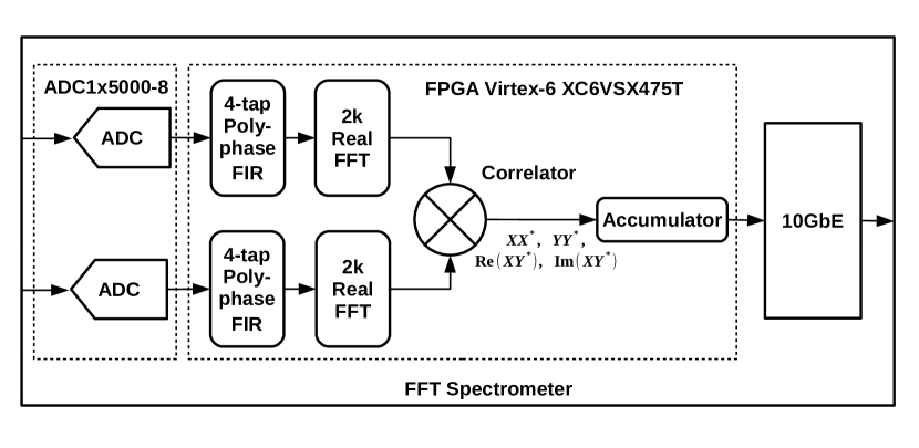
Figure 1: The spectrometer flowchart. The FX engine is implemented on FPGA chip, which use the polyphase filterbank to channelize the data and then do multiplication. The spectra is integrated and packetized into UDP packets. Each packet is then transmitted to the computer node using 10GbE fiber links.

We note that most of the RFI signals at KM40m are right-handed polarized. We only search for bursts in the left-handed polarization, but record the data from both polarisations. At NS26m, we search for bursts in the total intensity, i.e. the summation of two polarisations. The data is processed in real time, and only data with potential candidates of radio transients were recorded. The false alert probability of our detection threshold is $10^{-7}$ (cf. Section 2.3).

To save telescope resources, piggyback observations were carried out, i.e. we recorded the data while the telescopes were performing other observations. FRBs roughly distribute uniformly over the sky (Petroff et al., 2014), so such an observation mode does not in principle reduce the event rate significantly. In practice, however, a significant fraction of observing time, both at NS26m and KM40m, were allocated for pulsar observations. Observing along the Galactic plane may lead to a lower event rate (Petroff et al., 2014). We aimed to piggyback all observations at all available frequencies. By the time of writing this paper, due to the complexity in scheduling, we only piggybacked the 1.4 GHz observation at NS26m and 2.5 GHz observations at KM40m.

Table 1: The specifications for the Nanshan and the Kunming radio telescopes.

Name	$\Delta\Omega^{\ast}$	BW	$f_{\rm central}$	$f_{\rm ch}$	$\Delta t$	$G$	$T_{\rm sys}$
	sq. deg.	GHz	MHz	MHz	$\mu$s	K/Jy	K
NS26m	0.22	320	1.54	1.0	65	0.1	23
KM40m	0.04	140	2.24	1.0	65	0.23	70

^∗ Field of view

2.2 Digital backends

We recorded the data using home-brewed digital backends. It consists of a Fast-Fourier transform (FFT) spectrometer and recording computer. We built the FFT spectrometer based on the popular Roach2 platform, where a Virtex-6 family field programmable gate array (FPGA) of Xilinx performs digital signal processing and data packetizing. The FPGA gets the digitized signal from one 8-bit-5-Gsps analog-to-digital Converter (ADC) ADC1x5000-8 produced by E2V. In each ADC, there are four sampling cores. We configure the chip to sample the two polarisations at 2$\times$2 Gsps. We generate the ADC clock signal using Valon 5009 frequency synthesizer. The FPGA is fed with the same clock to form the sampling clock.

In the FPGA, 1024 channels are created using a polyphase filter bank (PFB) and then correlated to compute the coherency matrices, i.e. $\{XX^{*},YY^{*},{\rm Re}(XY^{*}),{\rm Im}(XY^{*})\}$, where $X$ and $Y$ are the complex voltage of the two polarizations, and $X^{*}$ and $Y^{*}$ are the corresponding complex conjugates. We integrate the coherency matrices for each of 64 samples, which results in a spectrum with time resolution of 65 $\mu$s. The data is then packetized and transferred to the recording computer node with the user datagram protocol (UDP) over a 10-Gigabit Ethernet (10 GbE) optical link. Figure 1 describes the hardware flowchart of our digital backend.

2.3 Realtime transient search and data analysis pipelines

For piggyback observations, we do not want to store all the data, since most of the data will not contain FRB signals. Also, in order to keep the data volume manageable, the data recording rate is limited and only data of candidates are stored. To do so, we implemented a realtime searching and data analysing pipeline.

Our realtime transient search system is called ‘Burst Emission Automatic Roger’ (bear), which has three major components, 1) the data processing manager (DPM), 2) the data buffering component (DBC), and 3) the data analysis component (DAC). The DBC captures the UDP packets from the 10 GbE optical link and buffers the data in the shared memory. The DAC firstly mitigates RFI, then de-disperses the signal at a given set of DM grids, searches for pulses using matched filter in the de-dispersed time series, and clusters the candidates to identify the burst events. There are multiple copies of the DAC processes running in the computer node to parallelize the data processing. The DPM allocates the shared memory on the data recording machine, and creates globally visible flags for each DAC task to coordinate the work. We will explain each parts separately in the following sections.

2.3.1 DBC, Data buffering

When the bear system starts, the DPM allocate 8 segments of shared memory in the data recording machine. DPM also creates globally visible flags for each of the 8 segments. Each flag has five states, namely, ‘empty’, ‘writing’, ‘ready’, ‘reading’, and ’saving’. After the shared memory is created, the initial flags are all set to ‘empty’ by the DPM.

The DBC captures the data from the 10 GbE optical link. It searches for the flags of ‘empty’. Once an ‘empty’ segment of the shared memory is found, the DBC changes the flag to ‘writing’ and starts to store the captured data into the corresponding memory block. The DBC changes the flag to ‘ready’ and seek for the next empty memory block, when the memory block is filled fully. The ‘ready’ flag notifies the DAC, then the DAC starts the data analysis after modifying the flag to ‘reading’. This prevents the DBC or other instances of DAC to interfere with the data processing. After DAC processes the data, the two possible flags are ‘saving’ or ‘empty’. If DAC finds candidates in the buffered data, the ‘saving’ flag is assigned, and DPM is notified to save the data to the hard disk. If no candidate is detected, the ‘empty’ flag is given, and memory block will be re-written by the DBC. Using this flag scheme, as far as the candidates rate is limited, we can even save the baseband data with a limited storage resource. For example, if we pick up candidates at a 5% probability, 500 Mbps file saving speed can handle incoming data with the rate of 10 Gbps. It is thus possible to do baseband data recording with only one computer node for FRB searching.

2.3.2 DAC, RFI mitigation

The first task of DAC is to mitigate the RFI signals in the data. Beside the common practice of zapping the channels with known persistent RFI (Fridman & Baan, 2001), we also perform the RFI mitigation called zero-DM matched filter, which effectively removes RFI of terrestrial origins (signal with nearly zero DM).

The zero-DM matched filter (ZDMF) is an improved version of the zero-DM filter (ZDF) developed by Eatough et al. (2009). The ZDF subtracts the zero-DM time series from the data, which significantly reduces the local RFI. In fact, the initial application of ZDF helped in the discovery of four new pulsars (Eatough et al., 2009), and has later been applied in several pulsar or single-pulse surveys (Eatough et al., 2013; Keane et al., 2010; Rane et al., 2016; Patel et al., 2018). The ZDMF estimates the waveform of the zero DM signal similarly to the ZDF, but subtracts only the corresponding contribution from each channel. Such a modification reduces the over-subtraction, when dealing with narrow-band RFI.

Similar to the zero-DM filter, the zero-DM time series (i.e. the ‘audio’ signal) is estimated by de-dispersing the original data at zero DM value. This is done by adding data of all frequency channels. The zero-DM waveform is denoted here as ${\boldsymbol{{s}}}_{\rm dm=0}$. We then estimate the corresponding contribution from each channel, i.e. we find the baseline $\beta_{i}$ and the scale factor $\alpha_{i}$ for each channel such that the residual of fitting the zero-DM waveform to the given channel is minimized. The residual $\chi^{2}$ is defined as

$$\chi^{2}=({\boldsymbol{{s}}}_{i}-\alpha_{i}{\boldsymbol{{s}}}_{\rm dm=0}-\beta_{i})^{2}\,,$$ (2)

where ${\boldsymbol{{s}}}_{i}$ is the time series of the $i$-th channel. The factor $\alpha_{i}$ can be found analytically as

$$\alpha_{i}=\frac{{\boldsymbol{{s}}}_{\rm dm=0}\cdot{\boldsymbol{{s}}}_{i}-\frac{1}{N}\sum s_{i}\sum s_{\rm dm=0}}{{\boldsymbol{{s}}}_{\rm dm=0}\cdot{\boldsymbol{{s}}}_{\rm dm=0}-\frac{1}{N}\sum s_{\rm dm=0}\sum s_{\rm dm=0}}\,.$$ (3)

Here, $\cdot$ is the inner product of the one dimensional time series. The symbol $\sum$ indicates the time domain summation with a total of $N$ data points. With the $\alpha_{i}$, we remove the RFI from the data using

$${\boldsymbol{{s}}}^{\prime}_{i}={\boldsymbol{{s}}}_{i}-\alpha_{i}{\boldsymbol{{s}}}_{\rm dm=0}\,,$$ (4)

where the new time series ${\boldsymbol{{s}}}^{\prime}_{i}$ is the data of the $i$-th channel with RFI removed. The DC-offset $\beta_{i}$ is not removed here, because it doesn’t affect the pulse detection.

Examples of our RFI mitigation are shown in Figure 2. The ZDMF can effectively remove RFI. The figure also shows the comparation between the ZDMF and ZDF.

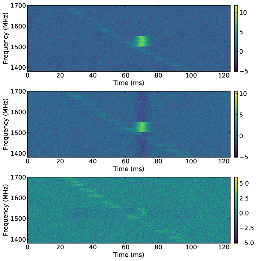
Figure 2: Examples for RFI mitigation algorithms. The top panel shows a simulated data set containing a highly frequency-modulated signal and a narrow-band RFI extended over a short duration, where the x-axis is the time, the y-axis is the observing frequency, and the colour/gray scale indicates signal strength. The middle panel shows the result after RFI mitigation using the ‘zero-DM’ technique (Eatough et al., 2009), where dips of intensity is introduced for channels containing no RFI. The bottom panel is the result using our ‘zero-DM matched filter’. The figures show that the current RFI mitigation works rather well, and only low level artifacts are left in the channels affected by the RFI.

2.3.3 DAC, De-dispersion and burst searching using matched filter

After RFI mitigation, we search for bursts in the data using the matched filter. Similarly to any matched filter for signal detection, if the parameter of the matched filter is slightly away from the ‘true’ value, there will be loss of signal-to-noise ratio (SNR). That is, if the true parameters of the FRB (DM, burst epoch, pulse width) is off the matched filter parameter grid, the detection probability becomes lower. As we will show below, we designed a nonlinear parameter searching grid, such that the SNR loss of bear is always smaller than a preset threshold. In this way, we minimize the number of trials needed for the matched filter.

In order to search for radio bursts of celestial origins, we need to align the data by correcting for the dispersion effect (c.f. Equation (1)). If the DM trial value is off the true value, the recovered burst becomes wider, extra noise is added to the burst, and the SNR of the burst signal reduces. If the DM offset is $\delta{\rm DM}$, the ratio between detection SNR and expected SNR is (Cordes & McLaughlin, 2003)

$$\frac{\rm SNR}{\rm SNR_{0}}=\frac{\sqrt{\pi}}{2}\zeta^{-1}\mathrm{erf}\zeta\,,$$ (5)

where $\rm SNR_{0}$ will be the SNR, if the true DM is used in searching and SNR is the observed SNR. The $\rm erf$ is the error function, and $\zeta$ is the ratio between the time delay caused by the DM offset and pulse width, i.e. $\zeta$ is

$$\zeta=6.91\times 10^{-3}\delta\mathrm{DM}\frac{\Delta\nu_{\mathrm{MHz}}}{W_{\mathrm{ms}}\nu_{\mathrm{GHz}}^{3}}\,,$$ (6)

where $W_{\rm ms}$ is the pulse width in units of millisecond, $\nu$ is the observing central frequency in GHz, and $\Delta\nu_{\rm MHz}$ is the bandwidth in MHz. If one uses decibel-scale SNR, denoted as $\cal S$, defined as ${\cal S}\equiv 10\log_{\rm 10}{\rm SNR}$ , Equation (5) which describes the SNR loss can be well approximated by

$$\Delta{\cal S}_{\rm dB}\simeq-\frac{5}{3}\zeta^{2}\,.$$ (7)

For our 1.5-GHz observation of 300 MHz bandwidth, the maximum allowable 15% SNR loss, i.e. -0.7 dB, constrains the DM searching grid to be uniform with a step of $1\ \rm cm^{-3}\,pc$. For high DM, the SNR loss caused by the intrachannel smearing will be dominant over the DM trial errors. One can use larger DM steps to reduce the computational cost. However, in order to also study the interferences with dispersive signatures and to simplify the data reduction, our DM trial grids span from 200 to 3000 $\mathrm{cm^{-3}\,pc}$ with 1 $\mathrm{cm^{-3}\ pc}$ increments. The SNR loss of the DM mismatch is plotted in Figure 3.

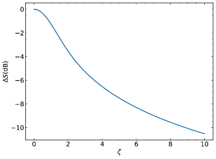
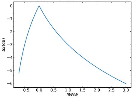
Figure 3: The SNR loss as the function of parameter mismatching. The y-axis is the SNR loss using a unit of log-10 based decibel. The upper panel is for the SNR loss due to mismatch of true and searching DM. The x-axis is the parameter $\eta$ defined in Equation (6). The lower panel is the SNR loss as function of width mismatch, where x-axis $\delta W/W$ is the fraction width of the pulse width mismatch.

As indicated by Equation (7), a preset SNR loss requires an uniform grid for DM trials. We use the subband de-dispersion algorithm (Magro et al., 2011) to de-disperse the data. The algorithm first divides the total $N$ channels into $N_{\rm sub}$ subbands, and de-disperses each subband over a coarse DM grid. Then the de-dispersed subband data is combined by another layer of de-dispersion to form the final de-dispersed 1-D time series on finer grid. For the optimal choice, this algorithm roughly speeds up the computations by factor of $\sqrt{N_{\rm sub}}$.

The in-channel dispersion smearing also introduces SNR loss. Such an effect is very similar to the DM mismatching loss. If we substitute the bandwidth $\Delta\nu$ with channel width and $\delta\rm DM$ with the DM in Equation (6), we can compute the SNR loss due to channel smearing. Our backend records with 1 MHz channel width, this leads to a maximum $-0.7\,{\rm dB}$ loss for pulse signal of 5 ms with $\rm DM=2000$.

We then search for burst signals in the de-dispersed 1-D time series using the matched filter technique. We assume the burst can be approximated by a square shaped wave, i.e. the template for the filter is

$$h(t;t_{0},w)=\left\{\begin{array}[]{l}A,\,{\rm if\,}|t-t_{0}|\leq W\\ 0,\,{\rm otherwise}\end{array}\right.,$$ (8)

where $A$, $t_{0}$, and $W$ are the amplitude, centre epoch and width of the square-shaped burst. The ‘most powerful test’, a statistical tool to detect signal with maximum detection probability with fixed false alarm probability, comes from the likelihood ratio test (Fisz, 1963). The detection statistic $S$ is the logarithmic likelihood ratio between the cases of having and not having the signal. As shown in the Appendix A, for the Gaussian noise case, one has

$$S=\frac{{\boldsymbol{{s}}}^{2}-({\boldsymbol{{s}}}-{\boldsymbol{{h}}})^{2}}{2\sigma^{2}}\,$$ (9)

where $\sigma$ is the standard deviation of the noise in 1-D time series. With the square wave filter (Equation (8)), Equation (9) is reduced to

$$S=\frac{1}{N_{\rm box}\sigma^{2}}\left(\sum_{|t-t0|\leq W}s(t)\right)^{2}\,,$$ (10)

where $N_{\rm box}$ is the number of data points in the time span where $|t-t_{0}|\leq W$. The likelihood ratio statistic $S$ is nothing but the square of the burst signal SNR, i.e.

$${\rm SNR}=\sqrt{S}\,.$$ (11)

We set the detection threshold $\gamma_{0}$, such that we will only record data when $S\geq\gamma_{0}$. For the null hypothesis, i.e. there is no burst in the data, the distribution of $S$ follows a $\chi^{2}$ distribution with one degree of freedom. The corresponding false alarm probability $P_{\rm FA}$ of the given threshold $\gamma_{0}$ is thus

$$P_{\rm FA}=\rm{erfc}\left(\sqrt{\frac{\gamma_{0}}{2}}\right)\simeq\sqrt{\frac{2}{\pi\gamma_{0}}}{\rm e}^{-\frac{\gamma_{0}}{2}}\,,$$ (12)

where function erfc is the complementary error function defined by ${\rm erfc}(x)\equiv 1-{\rm erf}(x)$. The approximation in the equation above is valid when $\gamma_{0}\gg 2$. In our searching pipeline, we use threshold of $P_{\rm FA}\leq 10^{-7}$, i.e. $\gamma_{0}\geq 28$. The approximation is therefore good enough to calculate the false alarm probability.

When there is a burst in the signal with a given SNR, the detection probability corresponding to the detection statistic $S$, i.e. the probability to get a $S$ larger than the threshold $\gamma_{0}$ is

$$P_{\rm D}=1-\frac{1}{2}\left[{\rm erf}\left(\frac{{\rm SNR}+\sqrt{\gamma_{0}}}{\sqrt{2}}\right)-{\rm erf}\left(\frac{{\rm SNR}-\sqrt{\gamma_{0}}}{\sqrt{2}}\right)\right]\,.$$ (13)

With the false alarm probability and detection probability, the statistical performance of the matched filter can be evaluated using the ‘receiver operating characteristic’ curves (ROC curves), it is the relation between $P_{\rm D}$ and $P_{\rm FA}$ parameterized using threshold $\gamma_{0}$. For reader’s reference, the ROC curves of the matched filter described here is given in Figure 4.

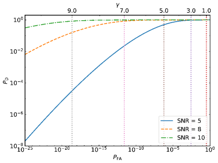
Figure 4: ROC curves for the matched filter using a square pulse waveform. The x-axis is the false alarm probability, and y-axis is the detection probability. The SNR of each curve is labelled in the figure. On the top of the panel, we also labelled the corresponding statistical threshold $\gamma_{0}$.

With the matched filter, we can now turn to problem of the equal-SNR-loss grid design for pulse width parameters $W$. The SNR loss with slightly wrong $t_{0}$ and $W$ becomes

$$\frac{\rm SNR}{\rm SNR_{0}}=\left\{\begin{array}[]{l}\frac{W}{W+\delta W},{\,\rm for\,}\delta W\geq 0\,,\\ \frac{W+\delta W}{W},{\,\rm for\,}\delta W<0\,.\end{array}\right.$$ (14)

where $\delta W$ is the mismatch of the pulse width. By setting the maximum SNR loss as 15%, the allowable grid for $W$ spans from $0.85W$ to $1.17W$. In this way, the equal-SNR-loss for the $k$-th grid should be a geometric series of $W_{k}=1.37^{k}W_{\rm min}$, and $W_{\rm min}$ is the minimum pulse width in the searching. Our minimum searching grid is 0.5 ms, and using only 12 grid steps cover the width search from 0.5 ms to 20 ms with a maximum SNR loss of 15%. The SNR loss and function of pulsar width mismatch is plotted in Figure 3.

The equal-SNR-loss grid for pulse epoch $t_{0}$ is a function of pulse width. If the equal-SNR-loss grid would be used for $t_{0}$, we would need to adjust it according to the pulse width grid. Luckily, due to a very efficient method to compute the statistic $S$, we can use a uniform-grid steps of 0.5 ms for $t_{0}$ in our searching. The $S$ is computed using the running averaging of data, which can be done very efficiently by subtracting one earlier data point and adding one new data point. In this way, the complexity of applying the square wave matched filter becomes of order $O(n)$ time complexity rather than well-known time complexity of order $O(n\log{}n)$ for applying the filters using the fast Fourier transform.

2.3.4 DAC, Clustering of candidates

By using de-dispersion, and matched filter, bear computes the detection statistic $S$ as a cube on a 3-D parameter grid spanned by DM, $W$ and $t_{0}$. bear reports detection, if the statistic $S$ is larger than the threshold $\gamma_{0}$. However, we note that naively reporting all the candidates with $S\geq\gamma_{0}$ is rather inefficient, as we need to remove the duplicated candidates.

Indeed, if the signal is strong, even in trials were with parameters mismatching the central values, the computed statistic still report detection. There will be many candidates clustering around the central peak of $S$. All those candidates in such a cluster are basically the same burst signal, but ‘found’ at slightly different parameters. We use the method called candidate clustering to remove such a redundancy.

Our recipe of candidates clustering is similar to the cleaning algorithm in the radio interferometry. The steps are as follows: 1) Find the grid with the highest value of $S$ in the detection statistics cube. 2) Find the neighbours of the grid with highest $S$. Here the ‘neighbours’ are the grids contacting the given central grids. 3) Find the neighbours of the neighbours, where each outer layer of neighbours has lower value of $S$ compared to the inner layer of neighbours. 4) Find the boundaries of all the neighbourhood region, where the boundaries are either confined by $S\geq\gamma_{0}$ or the requirements of monotonically decreasing $S$, 5) Report the central $S$ as one candidate, removing such the connected grid region, and repeating the procedure from the step 1. Here the monotonically decreasing $S$ ensures that interesting candidates do not get shadowed by other bright candidates nearby in the parameter grids.

With this procedure, we cluster the related candidates and the duplication of candidates is suppressed. Examples of the results will be given in the next section.

2.3.5 Test of pipelines

Our pipeline, from the home-brewed digital backends to the realtime searching is tested both in laboratory and on telescope site.

In the lab, we simulated the FRB radio frequency signal by modulating a wideband noise signal with low frequency pulses. The signal is fed to the backend and we check if the bear correctly detects the injected pulse. At the telescope sites, we tried to catch the single pulse stream from bright pulsars. We observed PSR B0329+54 at NS26m and the Vela pulsar at KM40m for 5 minutes. During the time, bright single bursts were detected and recorded. The candidate plots generated by the realtime searching pipeline is shown in Figure 5. The candidate plot also contains extra information to aid the users to do further inspection. The meaning of each panel is explained in the figure caption.

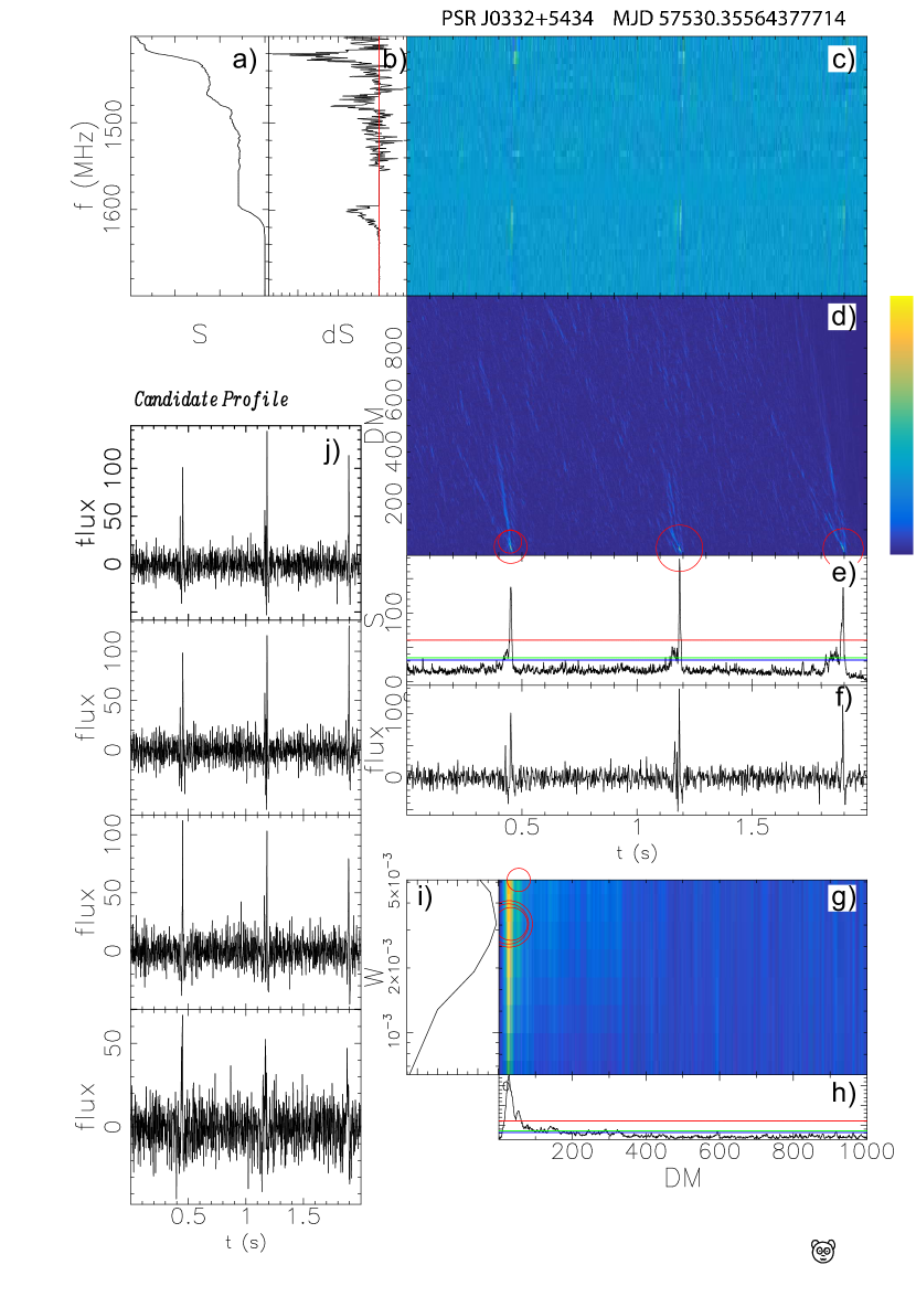
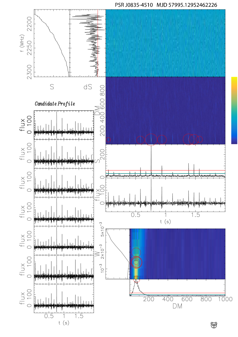
Figure 5: Left panel: The single pulse of PSR J0332+5434 detected at the NS26m. Right panel: The single pulse of J0835$-$4510 (Vela) detected at the KM40m. In the left panel, we also label each subplot with alphabet letters (a to h). The meaning of each subplots are, a) the integration of $S$ as function of frequency, b) the contribution of $S$ from each channel, c) filterbank data, the intensity as a function of frequency (y-axis) and time (x-axis), d) The $S$ as a function of DM (y-axis) and time (x-axis), e) $S$ as function of time, where red, green and blue horizontal lines (online version) correspondents to the $P_{\rm FA}$ of $10^{-7}$, $5\times 10^{-3}$, and $0.3$ respectively, f) de-dispersed 1-D time series of the highest $S$, g) $S$ as a function of width $W$ (y-axis) and DM (x-axis), h) $S$ as function of DM, i) $S$ as function of $W$, j) the pulse profile of each individual candidate. In the subplot c) the red circle indicates the location of each local maximum of $S$, which is the candidate reported in i). The size of the red circles are specified by the corresponding value of $S$, i.e. the SNR. As one can see, besides the local maxima indicated by the red circles, there are grids with values higher than the threshold. As shown in the subplot d) the $S$ around peak could still be higher than the red line. Our clustering algorithm combined the region around the peak and reduced the number of candidates reported in the subplot i).

3 Expectation of searching sensitivity and event rates for FRBs

In this section, we estimate the expected event rate of our experiment. At the time the current FRB searching project started, the event rate estimation for NS26m and KM40m was very uncertain. Most of the FRBs at that time were detected by the Parkes telescope. The sensitivity of Parkes is higher than both the NS26m and KM40m, but there is lack of information for the close-by FRB population, i.e. FRBs with higher flux. Thanks to the ASKAP survey (Shannon et al., 2018), we can now do a better estimation for the FRB event rate.

The minimum detection amplitude of FRB events is

$$S_{\mathrm{min}}=\beta\frac{\sqrt{\gamma_{0}}\ T_{\mathrm{sys}}}{G\sqrt{\mathrm{BW}\tau N_{\mathrm{p}}}},$$ (15)

where $S_{\mathrm{min}}$ is the minimum detectable flux for a given statistical threshold $\gamma_{0}$, $\beta\simeq 1$ is the digitisation factor, $\mathrm{BW}$ is the bandwidth, $N_{\mathrm{p}}$ is the number of polarisations, $\tau$ is the pulse width, $T_{\mathrm{sys}}$ is the system temperature and $G$ is the telescope gain. By choosing 3 ms as the reference width of FRB, the flux thresholds for SNR > 7 for NS26m and KM40m are 1.1 Jy and 3.3 Jy, respectively, using telescope parameters in Table 1.

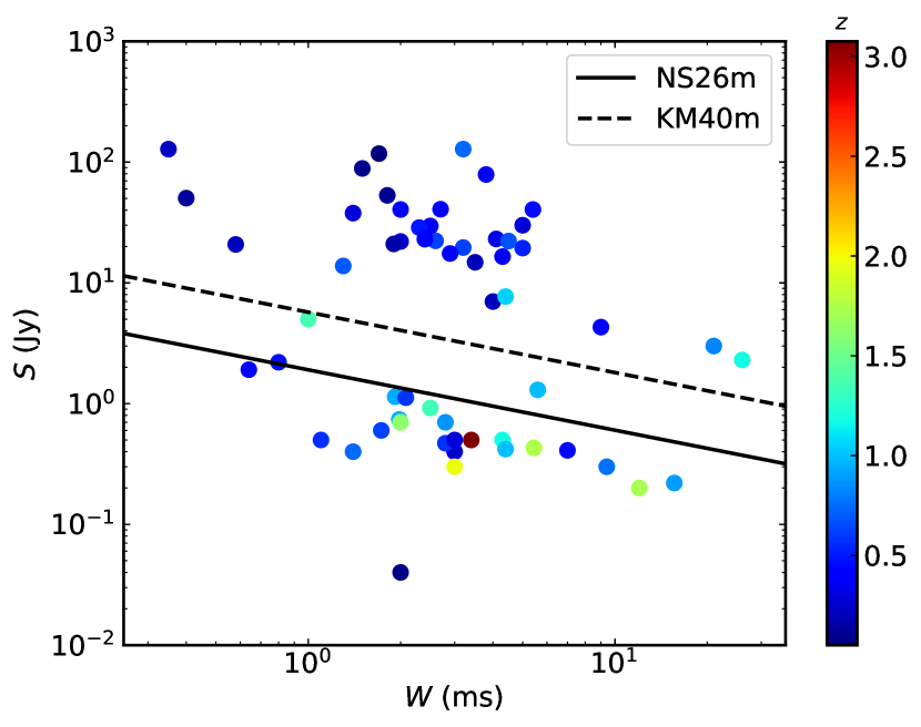
Figure 6: The currently known FRBs (coloured dots) together with the 7-$\sigma$ sensitivity of NS26m (solid line) and KM40m (dashed line). The x-axis is the FRB pulse width and the y-axis indicates the observed flux. The colour of each dot indicates the redshift estimated using the maximum-likelihood estimator of Luo et al. (2018). The data of known FRBs comes from the FRBCAT (Petroff et al., 2016). More than half of the known FRBs would be detectable with both the telescopes we used.

As shown in Figure 6, more than half of the known FRBs would be detected with NS26m and KM40m. Most of these detectable FRBs have redshift $z\leq 1$. Integrating over the cosmological comoving volume, the expected full-sky burst rate ($\rm BR$) in units of 1 per day per $4\pi$ solid angle is

$${\rm BR}=\int_{0}^{\infty}\phi(L)dL\int_{0}^{z_{\rm max}(L)}\frac{1}{1+z}\frac{dV}{dz}dz\,,$$ (16)

where $\phi(L)$ is the event rate luminosity function of FRBs in units of 1 per day per Mpc³ per luminosity ($L$) in the comoving frame. $z$ is the cosmological redshift. The $1+z$ factor in the denominator comes from the reduction of event rate for the observer on Earth due to the cosmological time dilation. The differential comoving volume ($dV/dz$) is

$$\frac{dV}{dz}=\frac{c}{H_{0}}\frac{1}{E(z)}\left(\frac{c}{H_{0}}\int_{0}^{z}\frac{1}{E(z)}dz\right)^{2}\,,$$ (17)

where the Hubble constant $H_{0}=67.8\,{\rm kms^{-1}Mpc^{-1}}$ (Planck Collaboration et al., 2018), $c$ is the light speed, and function $E(z)$ is the logarithmic time derivative of cosmic scale factor. With matter density $\Omega_{\rm m}=0.308$ and cosmological constant $\Omega_{\Lambda}=0.692$ (Planck Collaboration et al., 2018), one has

$$E(z)=\sqrt{\Omega_{\rm m}(1+z)^{3}+\Omega_{\rm Lambda}}\,.$$ (18)

The function $z_{\rm max}(L)$ is the maximum redshift of detectable FRBs with intrinsic luminosity $L$, i.e. it is defined implicitly via

$$L=4\pi r_{\rm L}(z_{\rm max})^{2}{\rm BW}S_{\rm min}\,,$$ (19)

where BW is the bandwidth of receiver at the Earth. $r_{\rm L}$ is the luminosity distance defined as

$$r_{\rm L}(z)=\frac{c(1+z)}{H_{\rm 0}}\int_{0}^{z}\frac{1}{E(z)}dz\,.$$ (20)

The normalized burst rate as function of the minimum detectable amplitude is shown in Figure 7.

Since the number density of FRB per comoving volume is not known (Luo et al., 2018), we can not directly compute the expected event rate ($\rm BR$) for a given telescope. We have to use the observed event rate at Parkes and the ratio between the expected event rate at our two telescopes to estimate the event rate at KM40m or NS26m. Here the ratio between the expected event rates of the two telescopes does not depend on the FRB number density anymore, as the number density is a normalisation factor and cancels out in the ratio. Denoting the observed event rate at the two telescopes as $\rho_{1}$ and $\rho_{2}$ (counts per day per full sky), we have

$$\rho_{2}=\frac{\rm BR_{2}}{\rm BR_{1}}\rho_{1}\,,$$ (21)

Clearly, the ratio $BR_{\rm 2}/BR_{\rm 1}$ becomes independent of the FRB number density, i.e. independent of $\int_{0}^{\infty}\phi(L)dL$.

The detection rate ($dN/dt$, i.e. counts per day) of a given telescope is

$$\frac{dN}{dt}=\frac{\rho N_{\rm b}\Delta\Omega}{4\pi}\,,$$ (22)

with $\Delta\Omega$ the solid angle of telescope main beam size, and $N_{\rm b}$ the number of beams. Based on the event rate of $10^{3}$ to $2\times 10^{4}$ $\rm sky^{-1}\,day^{-1}$ as seen by Parkes (Thornton et al., 2013), the event rate for NS26m is from $10^{-3}$ to $2\times 10^{-2}$ per day, i.e. 1 per 3 years to 1 per 50 days. The event rate at KM40m is rather tiny, and it falls in range of $[5\times 10^{-5},10^{-4}]$ per day, i.e. 1 per 50 years to 1 per 3 years. The derived event rates are comparable using the method in Chawla et al. (2017). Summing up, we expect one FRB on a monthly or yearly timescale for our current setups. Clearly, KM40m is not optimal for FRB searching due to the high temperature and narrow bandwidth, but we expect a better receiver frontend can significantly help the current situation.

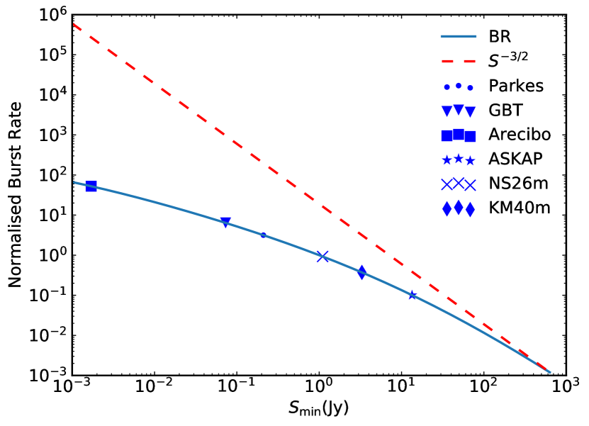
Figure 7: The normalized burst rate (see Equation (16)) as function of the minimum detectable amplitude. The solid blue curve is the computation made in this paper. Here, we normalize the burst rate arbitrarily to $S_{\rm min}=1$ Jy, as the event rate density of FRB in the Universe is rather uncertain. The red dashed curve is for $S_{\rm min}^{-3/2}$, i.e. the expected normalized burst rate in flat Euclidean space. One expects that the Euclidean approximation will be valid for FRBs located near the Earth. Indeed, the slope of the solid blue curve approaches $-3/2$, when $S_{\rm min}$ becomes large and observers can only see the near-by FRBs. We also compute the corresponding value of burst rate for a few other telescopes, which have detected FRBs, as indicated by the symbols on the solid blue curve. Telescope parameters are from Luo et al. (2018). Note that we use a beam-central gain of 10 ${\rm K/Jy}$ for Arecibo in the current computation to account for the sidelobe effects.

4 Discovery of the intriguing peryton

At the time this paper is written, we have observed for about 1600 hours at NS26m and 2400 hours at KM40m. So far no FRB has been found. However, an intriguing peryton was detected at NS26m.

On November 18th 2016, between UTC 02:24 to 03:31 (local time 18th November, 08:24 to 09:31), we detected a total of 218 broad-band radio pulses during pulsar timing observations, which show clear dispersion signature. The parameters of the pulsar timing observations are shown in Table 2. All the bursts have the same DM value of $531\pm 5\,{\rm cm^{-3}\,pc}$. An example candidate plot generated by bear is shown in Figure 8. The flux of each single burst is estimated as strong as 20 Jy.

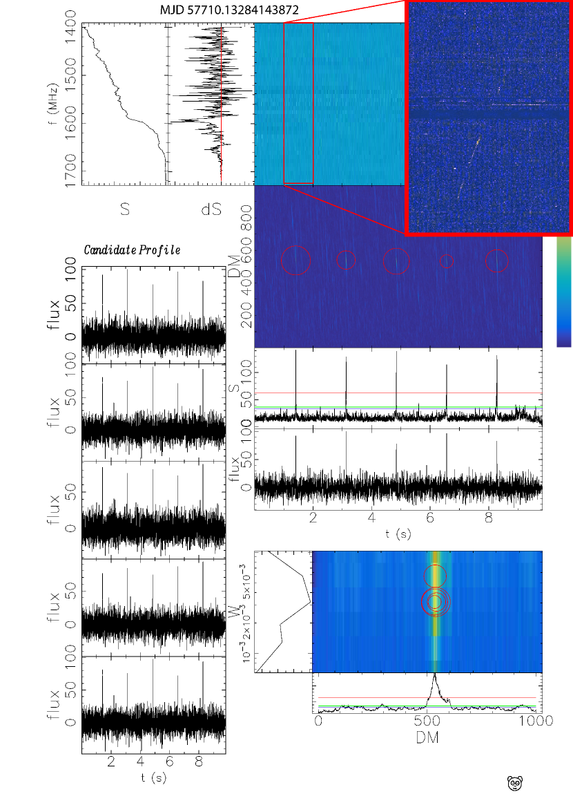
Figure 8: One of the peryton discovery plots generated by bear. The meaning of each panel is the same as Figure 5. The zoomed-in panel on the top-right corner shows the details of a single burst. One can see the dispersion feature rather clearly.

We found that the pulses spread across a 70-minute “burst window”. The occurrences of pulses fall into three major timespans. Six pulses were recorded in the first timespan, when the telescope was slewing from PSR J1509+5531 to PSR J1239+2453. The pulses appeared sporadically. After the first burst window, no pulse occurred until the 47-th minute, where the second timespan starts, which lasted for 15 minutes. In this timespan, the telescope was pointed at PSR J1041$-$1942 and 145 pulses were recorded. The third timespan started at the 55-th minute and lasted for 12 minutes, in which we recorded 67 pulses and the telescope was pointed at PSR J1012$-$2337.

Table 2: The parameters of the commensal pulsar timing observations, during which the peryton was detected.

Pulsar	RAJ	DECJ	Start date	Start time	Observation
	(hh:mm:ss)	(dd:mm:ss)	(dd-mm-yy)	(UTC)	duration (s)
J1509+5531	15:09:25.6	+55:31:32.4	2016-11-18	02:15:15	253
J1239+2453	12:39:40.4	+24:53:49.2	2016-11-18	02:26:25	367
J0953+0755	09:53:09.3	+07:55:35.8	2016-11-18	02:33:55	267
J1041$-$1942	10:41:36.1	-19:42:13.6	2016-11-18	02:39:15	975
J1041$-$1942	10:41:36.1	-19:42:13.6	2016-11-18	02:59:45	989
J1012$-$2337	10:12:33.7	-23:38:22.4	2016-11-18	03:16:35	989

The burst positions and the telescope trackings are shown in Figure 9. Since the telescope pointed in sky positions quite far apart from each other during the different detection timespans, one would expect the SNR to be drastically different if the pulsed signal originated from a single celestial position. The distribution of the SNRs of the pulses in different sky regions are shown in Figure 10. For a far-field source, we would expect more than $40$ dB variation between the pointing positions indicated in Figure 9, estimated using the propagation model after taking telescope structure reflection into account (Haslett, 2008). We do not see such large signal amplitude variations, which suggests that the pulsed signals do not come through the side lobes. The signal could potentially be understood in a scenario where it was picked up after the antenna feed, in which case the observed SNR would be roughly independent of the telescope pointing. However, this scenario requires an unlikely coincidence such that the signal is strong enough to overcome the approximately -90 dB isolation of coaxial cable and cavity for electronics and simultaneously not to be visible to the antenna feed. Otherwise we should detect a much stronger signal through the feed leakage. Thus, it appears more likely that the signal we report originates from local RFI.

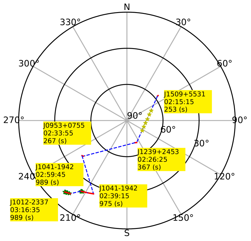
Figure 9: The orientation diagram with the occurrence altitude and azimuth angles of the pulses detected at the Nanshan radio telescope. The thick red lines represent the duration of the pulsar timing observations with the parameters shown in Table 2. The blue dash lines represent the telescope slewing to the next pulsar. The six yellow stars represent the 6 pulses detected during the telescope slewing without exact locations and the green stars represent the pulses detected during the pulsar trackings. The locations of the total pulses are shown in Table LABEL:tab:bursts. We have also labelled the pulsar name, the start time and duration of each pulsar timing observation.

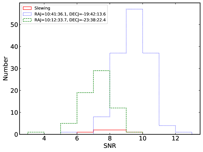
Figure 10: The histograms of the SNRs of the pulses in different sky locations.

We nevertheless studied the timing behavior of the pulses. Following the standard pulsar timing technique (e. g. Hobbs et al., 2006), we could measure and model the times-of-arrival (TOAs) of the pulses. We aligned a few of the most bright single pulses and then smoothed it to form the pulse profile template with psrchive (Hotan et al., 2004). After measuring the TOA of each single pulse, we used tempo2 (Hobbs et al., 2006) to build the timing model and calculate the timing residuals. The timing data indicate that the pulsed signal has a coherent timing behavior, where we can measure the period to a rather good precision ($p=1.71287\pm 0.00004$ s). The post-fitting timing residuals are shown in Figure 11, where only the pulse period is fitted. Since we detected no pulse between the first and the second observing window, it is unclear if the timing solution is still coherent for the first six data points. There seems to be a coherent solution for the second and third observing window. If we further fit for the period derivative, we get a value of $\dot{p}=3.50\times 10^{-6}\,{\rm s\,s^{-1}}$. From the Figure 11, we can see that over the last 20 minutes, the residual varies by 0.5 second. The mechanism therefore which generates such a periodicity in the pulses, must be stable in period to the $10^{-3}$ level.

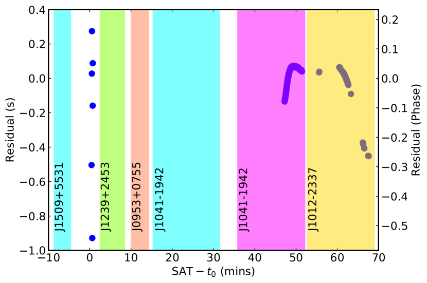
Figure 11: Timing residuals of the detected pulses. The x-axis shows the site arrival times (SATs) in units of minute, where the reference epoch is $t_{0}={\rm MJD\,57710.1}$. The y-axis are the timing residuals in units of second and in units of rotation phase. The shaded areas indicate the durations of pulsar timing observations.

In order to investigate how the RFI signals disguise themselves as celestial radio pulses, we measure the DM and dispersion index of each pulse, as shown in Table LABEL:tab:bursts. The dispersion index $\alpha$, as defined by the dispersive delay $\Delta t\propto\nu{{}^{-\alpha}}$, will be 2 for radio wave propagating in cold plasma (Manchester & Taylor, 1980). Such an index is widely used to check if pulses are of celestial origin (Burke-Spolaor et al., 2011; Petroff et al., 2015b). We use a Bayesian approach to fit for both DM and dispersion index simultaneously (Men et al., in prep). The measured DM and dispersion index are shown in Figure 12. As one can see, the DM values cluster around the central value of $530\,{\rm cm^{-3}\,pc}$. A clear variation of DM is also visible. The dispersion indices of this peryton are also varying. Intriguingly, the dispersion indices are around 2, and 17% of pulses have dispersion indices compatible with 2 within the 68% error-bar. The peryton would look like a true celestial source if only a small fraction of the pulses was detected. To our knowledge, such a type of peryton has never been reported before.

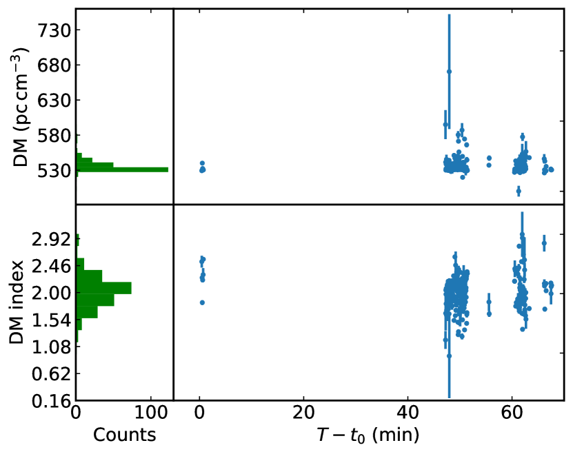
Figure 12: The DM and DM index for each single pulse. Top-left: The histogram of DM values, the x-axis is the number of counts, and the y-axis is the measured DM. Top-right: The time series of measures DM. The x-axis is the time in minutes with reference epoch $t_{0}={\rm MJD\,57710.1}$. Bottom-left, the histogram of DM index. Bottom-right, the time series of measures DM index. As one can see, the pulses have similar DM values, but a clear DM variation is detected. A significant fraction ($\sim 20\%$) of pulses are compatible with the cold plasma dispersion relation of DM index $\alpha=2$.

The peryton’s spectrum structure can be made more clearly after summing up individual pulses. The zoomed-in pulse is shown in Figure 13. The time-integrated pulse is double-peaked, and shows scintillation-like structures in the spectrum. Thanks to the high SNR of the summed pulse, we can see that the pulse is not perfectly aligned across frequency after de-dispersing with $\alpha=2$, which also suggest that the signal dispersion does not originate from the celestial cold plasma.

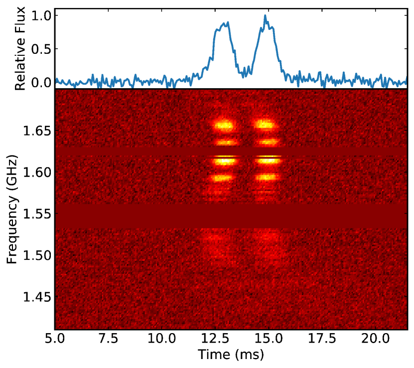
Figure 13: The perytons folded pulse. Top panel: the de-dispersed and folded pulse profile, where the x-axis is the time in units of millisecond and the y-axis is the relative flux. We can see a clear double-peaked profile with a total width of 4 ms. Bottom panel: the de-dispersed pulse as function of frequency (y-axis) and time (x-axis). There is a residual curvature in the pulse, i.e. the dispersion of the pulse does not follow the -2 index perfectly. The signal does not come from a celestial origin. There is also frequency modulation across the full band, which is visually similar to the scintillation behavior.

5 Discussions and Summary

This paper introduced the on-going FRB searching project using the Nanshan and Kunming radio telescopes. We described our searching hardware, software, data reduction algorithm and pipeline. We have computed the expected detection sensitivity and event rate of Nanshan and Kunming radio telescopes. For Nanshan, the sensitivity and event rate are 1.1 Jy and $10^{-3}$ to $2\times 10^{-2}$ per day. For Kunming, the numbers are 3.3 Jy and $5\times 10^{-5}$ to $10^{-4}$ per day. Based on the negative results in about $\rm 2400\ hrs\times\rm 0.04\ deg^{2}$ observations at S-band, we estimate a 95% confidence upper limit on the FRB rate of $R(S_{\mathrm{min}}=3.3\ \mathrm{Jy})<3.1\times 10^{4}\rm\ sky^{-1}day^{-1}$. This result agrees with the FRB rate reported in Burke-Spolaor et al. (2016).

We introduced our data processing pipeline, bear, where we start with the likelihood ratio test and get the same filter as the matched-filter theory. We also use the equal-SNR-loss scheme to set up the most economic parameter searching grid to save computational resources. As shown in Section 2.3, the setup is a logarithmic grid in pulse width and linear grids in DM and pulse epoch.

To this point, we have not yet detected any FRBs, but we have detected and studied an intriguing peryton. The peryton detected at Nanshan radio telescope differs drastically from previously reported perytons (Burke-Spolaor et al., 2011; Petroff et al., 2015b) and has nearly identical properties compared to most of the currently known FRBs. Unlike the common peryton width of 300 ms, our peryton burst has a double-peaked pulse profile and a 2-ms width. The DM value (531 $\rm pc\,cm^{-3}$) of the burst is also similar to the currently known FRB population. The inspection of individual single pulse gives dispersion index close to -2. All these key features fall in the middle of the FRB parameter space.

As shown in Figure 11, the peryton bursts lasted for a total of 70 minutes. Only six single bursts were detected in the first 45th minutes. In the rest of the observing window, i.e. from the 45 minutes to the 70th minutes, we detected very regular pulses with a period of 1.71287 s. It is highly likely that the phase of the bursts is coherent.

Two major reasons lead us to suggest that the bursts we see are likely to be RFI. Firstly, we detected significant deviations of the DM index after adding the single bursts. Secondly, the telescope pointing has moved towards different directions in the detection window. We could not trace the origin of the peryton and it never showed up again in subsequent observations. We searched all the available data and we continue paying attention for similar signals in our FRB searching campaign. Up to the time of writing the current paper, we found no other similar perytons.

With the available information, we did not conclude on a reasonable explanation for the peryton signal. A category of perytons has previously been identified to be generated from microwave ovens (Burke-Spolaor et al., 2011; Petroff et al., 2015b). Moreover, perytons with quasi-periodicity of an approximate 22-s cycle were also previously reported (Kocz et al., 2012). However, the peryton detected at Nanshan has remarkable different properties: 1) the pulses occurred in a more precise period; 2) the widths of the pulses are narrower, at $\sim$ 2 ms; 3) the DMs of the pulses are more concentrated, at $\sim 531\ \rm pc\,cm^{-3}$, and the DM index is very close to $-2$ as given by the cold plasma dispersion. Therefore, the peryton detected at Nanshan is likely to be a different type. It does not seem very probable that the signal originates from a microwave oven. There are two major types of microwave ovens, the transformer type and the inverter type (Matsumoto et al., 2003). For most of the transformer type ovens, the pulse width modulation for the microwave-oven power control operates with period longer than 10 s. For the inverter type, the conversion frequency is around several kHz. To the best of the author’s knowledge, periodic signal from microwave ovens similar to the peryton we discuss in this paper, was not previously reported (Anderson et al., 1979; Yamanaka & Shinozuka, 1995; Despres, 1997; Matsumoto et al., 2003). The signal is unlikely to originate from artificial satellite communication facilities or airplane, otherwise we should see such signals quite often. The lack of signal modulation also indicates that the burst may not be communication signals. We also made sure the signal is not due to instrumental instabilities or failure. Since we were piggybacking the pulsar observations, we can check if known pulsars are visible in the data. We found a single pulse with the correct DM of 9 $\rm{cm^{-3}\,pc}$ during observations of PSR J1239+2453 (Kazantsev & Potapov, 2017). The origin of the Nanshan peryton therefore remains unclear.

Our detected peryton mimics a real FRB signal. In fact, if only one or two single pulses were detected, one may had well concluded that the bursts are FRBs. We found that the DM index is critical to evaluate whether the burst is of celestial origin or not.

Figure 9 suggests that the apparent peryton positions on the sky may look like multiple isolated islands. Otherwise we would require the peryton to shut off from the 62th minute to the 65th minute as shown in Figure 11, while still keeping the coherent phase of timing. This suggests that the apparent directionality of near-field interference signals are rather complicated. For most of the FRB detection efforts, one relies on multibeam receivers to validate the celestial origin of burst signals. The idea is that near-field RFI can appear in multiple beams, while far-field true FRB signal appears only in adjacent beams. The indication of a complicated near-field pattern suggests that we should be more careful and may need extra information to validate the celestial origin of the pulsed signals.

Appendix A The likelihood ratio test statistic

The likelihood function is the probability distribution of data given the signal model. For the signal ${\boldsymbol{{s}}}$ of pure Gaussian white noise, the likelihood is

$$\Lambda_{\rm Null}=\frac{1}{(2\pi\sigma^{2})^{n/2}}{\rm e}^{-\frac{{\boldsymbol{{s}}}^{2}}{2\sigma^{2}}}\,,$$ (23)

where $n$ is the number of signal data points and $\sigma$ is the standard deviation of the noise. When there is a square wave signal on top of the Gaussian noise, the likelihood is

$$\Lambda_{\rm Null}=\frac{1}{(2\pi\sigma^{2})^{n/2}}{\rm e}^{-\frac{\left({\boldsymbol{{s}}}-{\boldsymbol{{h}}}\right)^{2}}{2\sigma^{2}}}\,,$$ (24)

The logarithm of the likelihood ratio between the cases of with and without a signal becomes

$$S\equiv\log\left(\frac{\Lambda_{\rm Sig}}{\Lambda_{\rm Null}}\right)\,,$$ (25)

which leads to Equation (9).

Table 3: The properties of the bursts from the peryton detected at Nanshan.

Burst	Date	Time	RAJ	DECJ	Telescope	Telescope	DM	DM index	SNR	Width
	(dd-mm-yy)	(UTC)	(hh:mm:ss)	(dd:mm:ss)	altitude (deg)	azimuth (deg)	($\rm pc\,cm^{-3}$)			(ms)
1	2016-11-18	02:24:26	–	–	–	–	529.3 $\pm$ 1.1	2.54 $\pm$ 0.10	6.4	2.0
2	2016-11-18	02:24:30	–	–	–	–	530.4 $\pm$ 1.1	2.27 $\pm$ 0.07	7.2	1.9
3	2016-11-18	02:24:32	–	–	–	–	540.1 $\pm$ 2.6	1.85 $\pm$ 0.04	9.2	1.9
4	2016-11-18	02:24:35	–	–	–	–	532.5 $\pm$ 0.5	2.23 $\pm$ 0.04	8.9	1.9
5	2016-11-18	02:24:41	–	–	–	–	530.9 $\pm$ 0.8	2.32 $\pm$ 0.11	9.3	1.9
6	2016-11-18	02:24:43	–	–	–	–	530.4 $\pm$ 0.8	2.58 $\pm$ 0.03	8.5	1.8
7	2016-11-18	03:11:13	10:41:36.1	-19:42:13.6	20.305	212.085	595.0 $\pm$ 20.6	1.22 $\pm$ 0.15	10.5	1.3
8	2016-11-18	03:11:15	10:41:36.1	-19:42:13.6	20.302	212.093	541.5 $\pm$ 5.6	1.67 $\pm$ 0.29	9.1	1.5
9	2016-11-18	03:11:17	10:41:36.1	-19:42:13.6	20.299	212.100	530.2 $\pm$ 0.8	2.06 $\pm$ 0.05	9.5	1.5
10	2016-11-18	03:11:18	10:41:36.1	-19:42:13.6	20.297	212.104	532.0 $\pm$ 0.9	1.99 $\pm$ 0.03	10.4	1.5
11	2016-11-18	03:11:20	10:41:36.1	-19:42:13.6	20.294	212.112	538.7 $\pm$ 1.6	1.83 $\pm$ 0.03	11.8	1.4
12	2016-11-18	03:11:22	10:41:36.1	-19:42:13.6	20.291	212.120	530.3 $\pm$ 1.1	2.09 $\pm$ 0.08	10.3	1.5
13	2016-11-18	03:11:24	10:41:36.1	-19:42:13.6	20.287	212.127	545.5 $\pm$ 6.5	1.64 $\pm$ 0.08	9.5	1.6
14	2016-11-18	03:11:25	10:41:36.1	-19:42:13.6	20.286	212.131	545.1 $\pm$ 1.8	1.72 $\pm$ 0.02	9.4	1.7
15	2016-11-18	03:11:27	10:41:36.1	-19:42:13.6	20.283	212.139	532.7 $\pm$ 1.0	1.98 $\pm$ 0.03	10.5	1.3
16	2016-11-18	03:11:29	10:41:36.1	-19:42:13.6	20.279	212.146	542.0 $\pm$ 5.2	1.72 $\pm$ 0.18	10.8	1.3
17	2016-11-18	03:11:30	10:41:36.1	-19:42:13.6	20.278	212.150	534.5 $\pm$ 0.9	1.98 $\pm$ 0.03	9.7	1.6
18	2016-11-18	03:11:32	10:41:36.1	-19:42:13.6	20.275	212.158	533.2 $\pm$ 0.6	2.14 $\pm$ 0.08	11.0	1.4
19	2016-11-18	03:11:34	10:41:36.1	-19:42:13.6	20.271	212.165	537.9 $\pm$ 1.9	1.81 $\pm$ 0.03	10.3	1.5
20	2016-11-18	03:11:36	10:41:36.1	-19:42:13.6	20.268	212.173	536.8 $\pm$ 1.7	1.83 $\pm$ 0.03	9.6	1.4
21	2016-11-18	03:11:37	10:41:36.1	-19:42:13.6	20.266	212.177	530.8 $\pm$ 0.5	2.16 $\pm$ 0.03	9.8	1.4
22	2016-11-18	03:11:39	10:41:36.1	-19:42:13.6	20.263	212.185	530.7 $\pm$ 0.9	2.00 $\pm$ 0.13	9.5	1.4
23	2016-11-18	03:11:41	10:41:36.1	-19:42:13.6	20.260	212.192	530.8 $\pm$ 0.6	2.07 $\pm$ 0.04	10.1	1.4
24	2016-11-18	03:11:42	10:41:36.1	-19:42:13.6	20.258	212.196	537.3 $\pm$ 1.8	1.79 $\pm$ 0.03	9.4	1.5
25	2016-11-18	03:11:44	10:41:36.1	-19:42:13.6	20.255	212.204	529.6 $\pm$ 0.5	2.21 $\pm$ 0.03	10.4	1.8
26	2016-11-18	03:11:46	10:41:36.1	-19:42:13.6	20.252	212.211	540.3 $\pm$ 6.2	1.74 $\pm$ 0.16	10.6	1.5
27	2016-11-18	03:11:48	10:41:36.1	-19:42:13.6	20.249	212.219	533.5 $\pm$ 0.8	2.02 $\pm$ 0.03	10.8	1.7
28	2016-11-18	03:11:49	10:41:36.1	-19:42:13.6	20.247	212.223	531.1 $\pm$ 0.6	2.08 $\pm$ 0.02	10.3	1.6
29	2016-11-18	03:11:51	10:41:36.1	-19:42:13.6	20.244	212.230	534.7 $\pm$ 1.9	1.91 $\pm$ 0.04	10.2	1.4
30	2016-11-18	03:11:53	10:41:36.1	-19:42:13.6	20.241	212.238	531.7 $\pm$ 1.2	1.95 $\pm$ 0.03	10.5	1.5
31	2016-11-18	03:11:54	10:41:36.1	-19:42:13.6	20.239	212.242	544.1 $\pm$ 2.7	1.66 $\pm$ 0.03	9.8	1.7
32	2016-11-18	03:11:56	10:41:36.1	-19:42:13.6	20.236	212.249	670.5 $\pm$ 81.9	0.95 $\pm$ 0.71	7.2	1.3
33	2016-11-18	03:11:58	10:41:36.1	-19:42:13.6	20.233	212.257	531.0 $\pm$ 0.8	2.16 $\pm$ 0.10	10.9	1.5
34	2016-11-18	03:12:00	10:41:36.1	-19:42:13.6	20.229	212.265	532.4 $\pm$ 1.2	1.95 $\pm$ 0.03	9.6	1.6
35	2016-11-18	03:12:01	10:41:36.1	-19:42:13.6	20.228	212.269	531.3 $\pm$ 0.7	2.06 $\pm$ 0.02	10.1	1.4
36	2016-11-18	03:12:03	10:41:36.1	-19:42:13.6	20.225	212.276	537.7 $\pm$ 1.5	1.82 $\pm$ 0.02	9.5	1.4
37	2016-11-18	03:12:05	10:41:36.1	-19:42:13.6	20.221	212.284	534.9 $\pm$ 2.1	1.93 $\pm$ 0.04	10.1	1.8
38	2016-11-18	03:12:07	10:41:36.1	-19:42:13.6	20.218	212.291	532.0 $\pm$ 1.4	2.04 $\pm$ 0.05	10.2	1.6
39	2016-11-18	03:12:08	10:41:36.1	-19:42:13.6	20.216	212.295	530.7 $\pm$ 0.5	2.14 $\pm$ 0.05	10.5	1.4
40	2016-11-18	03:12:10	10:41:36.1	-19:42:13.6	20.213	212.303	533.1 $\pm$ 0.9	2.11 $\pm$ 0.03	10.4	1.7
41	2016-11-18	03:12:12	10:41:36.1	-19:42:13.6	20.210	212.311	534.0 $\pm$ 1.1	1.99 $\pm$ 0.09	9.7	1.5
42	2016-11-18	03:12:13	10:41:36.1	-19:42:13.6	20.208	212.314	535.6 $\pm$ 1.9	1.86 $\pm$ 0.04	9.4	1.3
43	2016-11-18	03:12:15	10:41:36.1	-19:42:13.6	20.205	212.322	533.6 $\pm$ 1.4	1.98 $\pm$ 0.09	9.1	1.5
44	2016-11-18	03:12:17	10:41:36.1	-19:42:13.6	20.202	212.330	528.2 $\pm$ 0.6	2.12 $\pm$ 0.02	10.4	1.3
45	2016-11-18	03:12:19	10:41:36.1	-19:42:13.6	20.199	212.337	530.1 $\pm$ 0.8	2.12 $\pm$ 0.03	10.1	1.4
46	2016-11-18	03:12:20	10:41:36.1	-19:42:13.6	20.197	212.341	529.2 $\pm$ 0.7	2.06 $\pm$ 0.06	8.9	1.4
47	2016-11-18	03:12:22	10:41:36.1	-19:42:13.6	20.194	212.349	531.2 $\pm$ 0.5	2.21 $\pm$ 0.03	9.6	1.6
48	2016-11-18	03:12:24	10:41:36.1	-19:42:13.6	20.191	212.356	532.9 $\pm$ 0.7	2.15 $\pm$ 0.07	8.7	1.6
49	2016-11-18	03:12:25	10:41:36.1	-19:42:13.6	20.189	212.360	531.4 $\pm$ 0.7	2.18 $\pm$ 0.03	9.4	1.6
50	2016-11-18	03:12:27	10:41:36.1	-19:42:13.6	20.186	212.368	532.8 $\pm$ 1.3	1.93 $\pm$ 0.03	8.1	1.4
51	2016-11-18	03:12:29	10:41:36.1	-19:42:13.6	20.182	212.375	538.5 $\pm$ 4.2	1.79 $\pm$ 0.06	10.5	1.6
52	2016-11-18	03:12:31	10:41:36.1	-19:42:13.6	20.179	212.383	531.4 $\pm$ 6.1	2.04 $\pm$ 0.19	8.6	1.4
53	2016-11-18	03:12:32	10:41:36.1	-19:42:13.6	20.178	212.387	531.1 $\pm$ 0.5	2.22 $\pm$ 0.03	8.7	1.5
54	2016-11-18	03:12:34	10:41:36.1	-19:42:13.6	20.174	212.394	533.9 $\pm$ 1.7	1.89 $\pm$ 0.04	8.5	1.6
55	2016-11-18	03:12:37	10:41:36.1	-19:42:13.6	20.170	212.406	533.1 $\pm$ 1.1	1.98 $\pm$ 0.08	9.4	1.4
56	2016-11-18	03:12:39	10:41:36.1	-19:42:13.6	20.166	212.413	530.8 $\pm$ 1.2	2.11 $\pm$ 0.04	9.7	1.7
57	2016-11-18	03:12:41	10:41:36.1	-19:42:13.6	20.163	212.421	533.3 $\pm$ 2.3	1.95 $\pm$ 0.08	8.7	1.4
58	2016-11-18	03:12:43	10:41:36.1	-19:42:13.6	20.160	212.429	531.8 $\pm$ 0.7	2.12 $\pm$ 0.03	8.9	1.4
59	2016-11-18	03:12:44	10:41:36.1	-19:42:13.6	20.158	212.433	530.5 $\pm$ 0.7	2.07 $\pm$ 0.02	9.6	1.4
60	2016-11-18	03:12:46	10:41:36.1	-19:42:13.6	20.155	212.440	531.0 $\pm$ 0.5	2.30 $\pm$ 0.03	10.0	1.7
61	2016-11-18	03:12:48	10:41:36.1	-19:42:13.6	20.152	212.448	532.0 $\pm$ 2.7	2.07 $\pm$ 0.13	8.8	1.7
62	2016-11-18	03:12:49	10:41:36.1	-19:42:13.6	20.150	212.452	530.9 $\pm$ 0.5	2.17 $\pm$ 0.03	10.8	1.3
63	2016-11-18	03:12:51	10:41:36.1	-19:42:13.6	20.147	212.459	551.1 $\pm$ 3.5	1.55 $\pm$ 0.03	8.1	1.6
64	2016-11-18	03:12:53	10:41:36.1	-19:42:13.6	20.144	212.467	533.4 $\pm$ 3.1	1.89 $\pm$ 0.05	9.6	1.5
65	2016-11-18	03:12:55	10:41:36.1	-19:42:13.6	20.140	212.474	533.6 $\pm$ 1.6	1.95 $\pm$ 0.04	8.6	1.5
66	2016-11-18	03:12:56	10:41:36.1	-19:42:13.6	20.139	212.478	531.9 $\pm$ 0.8	2.12 $\pm$ 0.03	8.4	1.5
67	2016-11-18	03:12:58	10:41:36.1	-19:42:13.6	20.135	212.486	531.0 $\pm$ 0.5	2.20 $\pm$ 0.03	10.6	1.5
68	2016-11-18	03:13:00	10:41:36.1	-19:42:13.6	20.132	212.494	538.6 $\pm$ 1.8	1.91 $\pm$ 0.05	7.9	1.5
69	2016-11-18	03:13:01	10:41:36.1	-19:42:13.6	20.131	212.497	547.2 $\pm$ 1.9	2.62 $\pm$ 0.04	8.3	1.4
70	2016-11-18	03:13:03	10:41:36.1	-19:42:13.6	20.127	212.505	531.0 $\pm$ 0.5	2.17 $\pm$ 0.06	9.0	1.3
71	2016-11-18	03:13:05	10:41:36.1	-19:42:13.6	20.124	212.513	534.9 $\pm$ 2.9	1.89 $\pm$ 0.06	9.1	1.6
72	2016-11-18	03:13:07	10:41:36.1	-19:42:13.6	20.121	212.520	547.4 $\pm$ 3.5	1.63 $\pm$ 0.03	8.6	1.3
73	2016-11-18	03:13:08	10:41:36.1	-19:42:13.6	20.119	212.524	533.6 $\pm$ 1.7	2.27 $\pm$ 0.11	8.7	1.4
74	2016-11-18	03:13:10	10:41:36.1	-19:42:13.6	20.116	212.532	542.6 $\pm$ 5.2	2.48 $\pm$ 0.23	7.4	1.6
75	2016-11-18	03:13:12	10:41:36.1	-19:42:13.6	20.113	212.539	531.0 $\pm$ 1.0	2.20 $\pm$ 0.05	9.8	1.5
76	2016-11-18	03:13:13	10:41:36.1	-19:42:13.6	20.111	212.543	540.1 $\pm$ 2.8	1.72 $\pm$ 0.04	8.5	1.4
77	2016-11-18	03:13:15	10:41:36.1	-19:42:13.6	20.108	212.551	533.6 $\pm$ 1.4	1.81 $\pm$ 0.02	8.8	1.4
78	2016-11-18	03:13:17	10:41:36.1	-19:42:13.6	20.105	212.558	532.2 $\pm$ 0.8	2.14 $\pm$ 0.03	8.3	1.6
79	2016-11-18	03:13:19	10:41:36.1	-19:42:13.6	20.101	212.566	531.0 $\pm$ 0.5	2.18 $\pm$ 0.03	9.7	1.4
80	2016-11-18	03:13:20	10:41:36.1	-19:42:13.6	20.100	212.570	532.8 $\pm$ 0.8	2.09 $\pm$ 0.06	8.9	1.4
81	2016-11-18	03:13:22	10:41:36.1	-19:42:13.6	20.096	212.577	534.8 $\pm$ 1.0	2.07 $\pm$ 0.04	10.0	1.5
82	2016-11-18	03:13:24	10:41:36.1	-19:42:13.6	20.093	212.585	536.4 $\pm$ 0.8	2.20 $\pm$ 0.05	7.7	1.5
83	2016-11-18	03:13:25	10:41:36.1	-19:42:13.6	20.092	212.589	535.2 $\pm$ 1.5	1.95 $\pm$ 0.03	9.4	1.5
84	2016-11-18	03:13:27	10:41:36.1	-19:42:13.6	20.088	212.596	533.8 $\pm$ 2.9	1.84 $\pm$ 0.05	8.7	1.5
85	2016-11-18	03:13:29	10:41:36.1	-19:42:13.6	20.085	212.604	537.2 $\pm$ 2.5	1.87 $\pm$ 0.10	9.4	1.5
86	2016-11-18	03:13:30	10:41:36.1	-19:42:13.6	20.083	212.608	531.8 $\pm$ 1.2	2.03 $\pm$ 0.05	9.1	1.5
87	2016-11-18	03:13:32	10:41:36.1	-19:42:13.6	20.080	212.615	535.9 $\pm$ 1.5	2.31 $\pm$ 0.11	8.8	1.4
88	2016-11-18	03:13:34	10:41:36.1	-19:42:13.6	20.077	212.623	530.6 $\pm$ 1.6	2.10 $\pm$ 0.08	8.8	1.4
89	2016-11-18	03:13:36	10:41:36.1	-19:42:13.6	20.074	212.631	550.2 $\pm$ 3.4	1.52 $\pm$ 0.03	8.5	1.4
90	2016-11-18	03:13:37	10:41:36.1	-19:42:13.6	20.072	212.634	531.8 $\pm$ 0.9	2.15 $\pm$ 0.07	9.2	1.5
91	2016-11-18	03:13:39	10:41:36.1	-19:42:13.6	20.069	212.642	580.5 $\pm$ 5.3	1.31 $\pm$ 0.03	8.7	1.5
92	2016-11-18	03:13:41	10:41:36.1	-19:42:13.6	20.065	212.650	533.9 $\pm$ 0.5	2.24 $\pm$ 0.03	9.2	1.5
93	2016-11-18	03:13:42	10:41:36.1	-19:42:13.6	20.064	212.653	571.3 $\pm$ 0.8	1.36 $\pm$ 0.00	8.5	1.6
94	2016-11-18	03:13:44	10:41:36.1	-19:42:13.6	20.061	212.661	540.1 $\pm$ 0.9	2.41 $\pm$ 0.06	9.0	1.6
95	2016-11-18	03:13:46	10:41:36.1	-19:42:13.6	20.057	212.669	532.1 $\pm$ 0.8	2.01 $\pm$ 0.02	9.5	1.3
96	2016-11-18	03:13:48	10:41:36.1	-19:42:13.6	20.054	212.676	556.0 $\pm$ 3.2	1.51 $\pm$ 0.03	8.6	1.4
97	2016-11-18	03:13:49	10:41:36.1	-19:42:13.6	20.052	212.680	539.6 $\pm$ 2.6	1.71 $\pm$ 0.03	9.4	1.4
98	2016-11-18	03:13:51	10:41:36.1	-19:42:13.6	20.049	212.688	546.1 $\pm$ 3.6	1.66 $\pm$ 0.04	8.8	1.7
99	2016-11-18	03:13:53	10:41:36.1	-19:42:13.6	20.046	212.695	533.2 $\pm$ 1.2	2.03 $\pm$ 0.06	9.8	1.6
100	2016-11-18	03:13:54	10:41:36.1	-19:42:13.6	20.044	212.699	539.1 $\pm$ 2.8	1.71 $\pm$ 0.04	9.1	1.4
101	2016-11-18	03:13:56	10:41:36.1	-19:42:13.6	20.041	212.707	541.5 $\pm$ 2.7	1.72 $\pm$ 0.03	9.7	1.6
102	2016-11-18	03:13:58	10:41:36.1	-19:42:13.6	20.038	212.714	530.9 $\pm$ 0.9	2.18 $\pm$ 0.04	9.8	1.7
103	2016-11-18	03:14:00	10:41:36.1	-19:42:13.6	20.034	212.722	531.3 $\pm$ 0.5	2.19 $\pm$ 0.03	9.2	1.4
104	2016-11-18	03:14:01	10:41:36.1	-19:42:13.6	20.033	212.726	536.9 $\pm$ 2.1	1.75 $\pm$ 0.30	8.6	1.4
105	2016-11-18	03:14:03	10:41:36.1	-19:42:13.6	20.029	212.733	539.0 $\pm$ 2.1	1.72 $\pm$ 0.03	9.7	1.2
106	2016-11-18	03:14:05	10:41:36.1	-19:42:13.6	20.026	212.741	539.1 $\pm$ 0.3	2.36 $\pm$ 0.02	8.8	1.4
107	2016-11-18	03:14:06	10:41:36.1	-19:42:13.6	20.025	212.745	536.3 $\pm$ 4.8	1.83 $\pm$ 0.23	7.5	1.4
108	2016-11-18	03:14:08	10:41:36.1	-19:42:13.6	20.021	212.752	538.4 $\pm$ 3.7	1.75 $\pm$ 0.11	8.5	1.6
109	2016-11-18	03:14:10	10:41:36.1	-19:42:13.6	20.018	212.760	532.3 $\pm$ 1.4	1.90 $\pm$ 0.03	8.4	1.4
110	2016-11-18	03:14:12	10:41:36.1	-19:42:13.6	20.015	212.768	535.3 $\pm$ 1.7	1.88 $\pm$ 0.04	9.4	1.6
111	2016-11-18	03:14:13	10:41:36.1	-19:42:13.6	20.013	212.771	537.4 $\pm$ 3.2	1.82 $\pm$ 0.07	9.8	1.4
112	2016-11-18	03:14:15	10:41:36.1	-19:42:13.6	20.010	212.779	532.4 $\pm$ 1.0	2.05 $\pm$ 0.03	10.8	1.5
113	2016-11-18	03:14:17	10:41:36.1	-19:42:13.6	20.007	212.787	531.0 $\pm$ 0.6	2.10 $\pm$ 0.03	11.6	1.3
114	2016-11-18	03:14:18	10:41:36.1	-19:42:13.6	20.005	212.790	532.2 $\pm$ 0.5	2.18 $\pm$ 0.03	10.3	1.6
115	2016-11-18	03:14:20	10:41:36.1	-19:42:13.6	20.002	212.798	530.8 $\pm$ 1.5	1.98 $\pm$ 0.04	7.9	1.4
116	2016-11-18	03:14:22	10:41:36.1	-19:42:13.6	19.998	212.806	531.2 $\pm$ 2.2	1.95 $\pm$ 0.11	8.8	1.5
117	2016-11-18	03:14:24	10:41:36.1	-19:42:13.6	19.995	212.813	587.1 $\pm$ 10.0	1.28 $\pm$ 0.05	8.7	1.4
118	2016-11-18	03:14:25	10:41:36.1	-19:42:13.6	19.993	212.817	533.1 $\pm$ 2.1	2.11 $\pm$ 0.12	9.6	1.6
119	2016-11-18	03:14:27	10:41:36.1	-19:42:13.6	19.990	212.825	533.1 $\pm$ 0.5	2.26 $\pm$ 0.03	10.3	1.6
120	2016-11-18	03:14:29	10:41:36.1	-19:42:13.6	19.987	212.832	549.7 $\pm$ 3.0	1.56 $\pm$ 0.03	9.9	1.5
121	2016-11-18	03:14:30	10:41:36.1	-19:42:13.6	19.985	212.836	519.9 $\pm$ 0.2	2.00 $\pm$ 0.00	7.7	6.5
122	2016-11-18	03:14:32	10:41:36.1	-19:42:13.6	19.982	212.844	533.5 $\pm$ 1.8	1.92 $\pm$ 0.07	9.5	1.6
123	2016-11-18	03:14:34	10:41:36.1	-19:42:13.6	19.979	212.851	530.8 $\pm$ 1.0	2.04 $\pm$ 0.03	10.2	1.5
124	2016-11-18	03:14:36	10:41:36.1	-19:42:13.6	19.975	212.859	530.9 $\pm$ 1.4	1.97 $\pm$ 0.03	8.9	1.5
125	2016-11-18	03:14:37	10:41:36.1	-19:42:13.6	19.974	212.862	541.4 $\pm$ 2.1	1.70 $\pm$ 0.03	10.0	1.5
126	2016-11-18	03:14:39	10:41:36.1	-19:42:13.6	19.970	212.870	531.6 $\pm$ 0.8	2.06 $\pm$ 0.03	10.7	1.6
127	2016-11-18	03:14:41	10:41:36.1	-19:42:13.6	19.967	212.878	538.0 $\pm$ 3.6	1.78 $\pm$ 0.09	9.4	1.4
128	2016-11-18	03:14:42	10:41:36.1	-19:42:13.6	19.966	212.881	532.9 $\pm$ 1.2	2.33 $\pm$ 0.15	9.1	1.5
129	2016-11-18	03:14:44	10:41:36.1	-19:42:13.6	19.962	212.889	533.3 $\pm$ 1.4	1.90 $\pm$ 0.04	9.6	1.5
130	2016-11-18	03:14:46	10:41:36.1	-19:42:13.6	19.959	212.897	533.3 $\pm$ 2.1	1.93 $\pm$ 0.05	9.3	1.4
131	2016-11-18	03:14:48	10:41:36.1	-19:42:13.6	19.956	212.904	540.6 $\pm$ 2.8	1.76 $\pm$ 0.06	9.3	1.4
132	2016-11-18	03:14:49	10:41:36.1	-19:42:13.6	19.954	212.908	531.1 $\pm$ 1.4	2.07 $\pm$ 0.04	10.9	1.7
133	2016-11-18	03:14:51	10:41:36.1	-19:42:13.6	19.951	212.916	529.2 $\pm$ 0.5	2.24 $\pm$ 0.05	10.6	1.7
134	2016-11-18	03:14:53	10:41:36.1	-19:42:13.6	19.947	212.923	574.5 $\pm$ 2.5	1.39 $\pm$ 0.01	9.4	1.7
135	2016-11-18	03:14:56	10:41:36.1	-19:42:13.6	19.943	212.935	529.3 $\pm$ 0.7	2.16 $\pm$ 0.03	11.0	1.7
136	2016-11-18	03:14:58	10:41:36.1	-19:42:13.6	19.939	212.942	532.0 $\pm$ 1.0	2.02 $\pm$ 0.03	10.8	1.5
137	2016-11-18	03:15:00	10:41:36.1	-19:42:13.6	19.936	212.950	531.1 $\pm$ 0.7	2.30 $\pm$ 0.07	10.5	1.8
138	2016-11-18	03:15:01	10:41:36.1	-19:42:13.6	19.934	212.954	529.0 $\pm$ 0.5	2.21 $\pm$ 0.03	9.7	1.8
139	2016-11-18	03:15:03	10:41:36.1	-19:42:13.6	19.931	212.961	534.3 $\pm$ 2.7	1.86 $\pm$ 0.07	8.6	1.6
140	2016-11-18	03:15:05	10:41:36.1	-19:42:13.6	19.928	212.969	530.8 $\pm$ 0.4	2.23 $\pm$ 0.03	10.6	1.5
141	2016-11-18	03:15:06	10:41:36.1	-19:42:13.6	19.926	212.973	529.2 $\pm$ 6.5	2.07 $\pm$ 0.18	9.9	1.5
142	2016-11-18	03:15:08	10:41:36.1	-19:42:13.6	19.923	212.980	530.0 $\pm$ 4.6	2.05 $\pm$ 0.17	9.6	1.4
143	2016-11-18	03:15:10	10:41:36.1	-19:42:13.6	19.919	212.988	531.4 $\pm$ 0.8	2.10 $\pm$ 0.04	12.0	1.6
144	2016-11-18	03:15:12	10:41:36.1	-19:42:13.6	19.916	212.995	534.4 $\pm$ 1.3	1.94 $\pm$ 0.03	9.4	1.7
145	2016-11-18	03:15:13	10:41:36.1	-19:42:13.6	19.915	212.999	528.9 $\pm$ 0.4	2.25 $\pm$ 0.03	9.7	1.6
146	2016-11-18	03:15:15	10:41:36.1	-19:42:13.6	19.911	213.007	530.8 $\pm$ 0.6	2.29 $\pm$ 0.05	7.6	1.7
147	2016-11-18	03:15:17	10:41:36.1	-19:42:13.6	19.908	213.014	566.2 $\pm$ 3.5	1.50 $\pm$ 0.03	9.6	1.8
148	2016-11-18	03:15:18	10:41:36.1	-19:42:13.6	19.906	213.018	545.0 $\pm$ 3.9	1.65 $\pm$ 0.05	8.4	1.3
149	2016-11-18	03:15:20	10:41:36.1	-19:42:13.6	19.903	213.026	544.6 $\pm$ 2.6	1.68 $\pm$ 0.03	8.8	1.7
150	2016-11-18	03:15:22	10:41:36.1	-19:42:13.6	19.900	213.033	530.9 $\pm$ 0.5	2.37 $\pm$ 0.03	5.8	1.6
151	2016-11-18	03:15:25	10:41:36.1	-19:42:13.6	19.895	213.045	529.6 $\pm$ 0.5	2.34 $\pm$ 0.04	9.6	1.7
152	2016-11-18	03:19:34	10:12:33.7	-23:38:22.4	12.900	218.329	537.2 $\pm$ 1.7	1.86 $\pm$ 0.15	7.1	1.7
153	2016-11-18	03:19:37	10:12:33.7	-23:38:22.4	12.895	218.339	547.3 $\pm$ 3.8	1.66 $\pm$ 0.05	7.5	1.3
154	2016-11-18	03:24:28	10:12:33.7	-23:38:22.4	12.344	219.329	527.1 $\pm$ 0.6	2.21 $\pm$ 0.03	6.3	1.6
155	2016-11-18	03:24:30	10:12:33.7	-23:38:22.4	12.341	219.336	529.9 $\pm$ 0.9	2.21 $\pm$ 0.04	6.0	1.7
156	2016-11-18	03:24:32	10:12:33.7	-23:38:22.4	12.337	219.342	531.8 $\pm$ 2.1	2.42 $\pm$ 0.14	7.4	0.7
157	2016-11-18	03:24:37	10:12:33.7	-23:38:22.4	12.327	219.359	531.6 $\pm$ 0.7	2.39 $\pm$ 0.05	7.7	2.1
158	2016-11-18	03:24:42	10:12:33.7	-23:38:22.4	12.318	219.376	543.3 $\pm$ 2.3	1.79 $\pm$ 0.03	6.8	1.4
159	2016-11-18	03:24:45	10:12:33.7	-23:38:22.4	12.312	219.386	530.4 $\pm$ 0.9	2.41 $\pm$ 0.06	6.2	1.6
160	2016-11-18	03:24:49	10:12:33.7	-23:38:22.4	12.304	219.400	538.1 $\pm$ 2.4	1.85 $\pm$ 0.04	8.3	1.6
161	2016-11-18	03:25:04	10:12:33.7	-23:38:22.4	12.276	219.451	535.5 $\pm$ 2.2	1.91 $\pm$ 0.04	7.2	1.4
162	2016-11-18	03:25:08	10:12:33.7	-23:38:22.4	12.268	219.464	528.5 $\pm$ 0.8	2.33 $\pm$ 0.07	5.7	1.9
163	2016-11-18	03:25:09	10:12:33.7	-23:38:22.4	12.266	219.468	539.6 $\pm$ 6.3	1.85 $\pm$ 0.16	8.4	1.6
164	2016-11-18	03:25:16	10:12:33.7	-23:38:22.4	12.253	219.491	500.2 $\pm$ 7.6	1.76 $\pm$ 0.09	3.9	3.5
165	2016-11-18	03:25:18	10:12:33.7	-23:38:22.4	12.249	219.498	529.8 $\pm$ 0.7	2.44 $\pm$ 0.06	9.8	1.5
166	2016-11-18	03:25:21	10:12:33.7	-23:38:22.4	12.243	219.508	542.2 $\pm$ 1.6	2.80 $\pm$ 0.04	7.2	1.8
167	2016-11-18	03:25:25	10:12:33.7	-23:38:22.4	12.235	219.522	545.6 $\pm$ 1.9	1.73 $\pm$ 0.02	7.5	1.6
168	2016-11-18	03:25:26	10:12:33.7	-23:38:22.4	12.233	219.525	542.7 $\pm$ 9.7	1.77 $\pm$ 0.11	7.9	1.8
169	2016-11-18	03:25:28	10:12:33.7	-23:38:22.4	12.230	219.532	532.8 $\pm$ 1.7	2.10 $\pm$ 0.21	6.9	1.4
170	2016-11-18	03:25:30	10:12:33.7	-23:38:22.4	12.226	219.539	537.2 $\pm$ 2.7	1.85 $\pm$ 0.05	7.3	1.6
171	2016-11-18	03:25:32	10:12:33.7	-23:38:22.4	12.222	219.545	526.6 $\pm$ 1.6	2.16 $\pm$ 0.07	6.4	1.6
172	2016-11-18	03:25:33	10:12:33.7	-23:38:22.4	12.220	219.549	529.2 $\pm$ 4.0	2.06 $\pm$ 0.08	7.8	1.7
173	2016-11-18	03:25:35	10:12:33.7	-23:38:22.4	12.216	219.555	528.0 $\pm$ 0.6	2.25 $\pm$ 0.05	6.7	1.7
174	2016-11-18	03:25:37	10:12:33.7	-23:38:22.4	12.212	219.562	534.5 $\pm$ 2.7	1.98 $\pm$ 0.08	7.9	1.5
175	2016-11-18	03:25:38	10:12:33.7	-23:38:22.4	12.210	219.566	531.6 $\pm$ 1.6	2.00 $\pm$ 0.04	8.3	1.6
176	2016-11-18	03:25:40	10:12:33.7	-23:38:22.4	12.206	219.572	531.4 $\pm$ 0.9	2.06 $\pm$ 0.12	7.7	1.7
177	2016-11-18	03:25:44	10:12:33.7	-23:38:22.4	12.199	219.586	533.5 $\pm$ 1.7	1.94 $\pm$ 0.04	8.9	1.8
178	2016-11-18	03:25:45	10:12:33.7	-23:38:22.4	12.197	219.589	535.8 $\pm$ 3.8	1.86 $\pm$ 0.07	6.9	1.8
179	2016-11-18	03:25:47	10:12:33.7	-23:38:22.4	12.193	219.596	531.5 $\pm$ 2.5	2.03 $\pm$ 0.09	6.9	1.5
180	2016-11-18	03:25:49	10:12:33.7	-23:38:22.4	12.189	219.603	530.4 $\pm$ 0.7	2.54 $\pm$ 0.03	8.1	1.6
181	2016-11-18	03:25:50	10:12:33.7	-23:38:22.4	12.187	219.606	528.7 $\pm$ 1.3	2.10 $\pm$ 0.06	7.5	1.6
182	2016-11-18	03:25:54	10:12:33.7	-23:38:22.4	12.180	219.620	550.8 $\pm$ 2.7	1.67 $\pm$ 0.03	6.1	1.6
183	2016-11-18	03:25:55	10:12:33.7	-23:38:22.4	12.178	219.623	538.0 $\pm$ 1.6	1.85 $\pm$ 0.03	7.9	1.2
184	2016-11-18	03:25:57	10:12:33.7	-23:38:22.4	12.174	219.630	553.0 $\pm$ 14.5	3.00 $\pm$ 0.38	5.5	1.1
185	2016-11-18	03:25:59	10:12:33.7	-23:38:22.4	12.170	219.636	546.9 $\pm$ 1.6	2.94 $\pm$ 0.03	5.5	1.5
186	2016-11-18	03:26:01	10:12:33.7	-23:38:22.4	12.166	219.643	577.5 $\pm$ 5.8	1.40 $\pm$ 0.04	6.2	1.5
187	2016-11-18	03:26:02	10:12:33.7	-23:38:22.4	12.164	219.647	535.9 $\pm$ 2.2	1.92 $\pm$ 0.05	8.7	1.5
188	2016-11-18	03:26:04	10:12:33.7	-23:38:22.4	12.160	219.653	534.6 $\pm$ 1.4	1.91 $\pm$ 0.03	8.0	1.8
189	2016-11-18	03:26:06	10:12:33.7	-23:38:22.4	12.157	219.660	548.9 $\pm$ 2.9	1.66 $\pm$ 0.03	8.1	1.8
190	2016-11-18	03:26:07	10:12:33.7	-23:38:22.4	12.155	219.663	528.2 $\pm$ 2.7	2.10 $\pm$ 0.06	5.8	1.3
191	2016-11-18	03:26:09	10:12:33.7	-23:38:22.4	12.151	219.670	536.4 $\pm$ 4.3	1.86 $\pm$ 0.07	8.4	2.0
192	2016-11-18	03:26:11	10:12:33.7	-23:38:22.4	12.147	219.677	535.2 $\pm$ 3.6	2.66 $\pm$ 0.17	7.8	1.9
193	2016-11-18	03:26:13	10:12:33.7	-23:38:22.4	12.143	219.684	533.8 $\pm$ 1.5	1.98 $\pm$ 0.16	7.2	1.3
194	2016-11-18	03:26:14	10:12:33.7	-23:38:22.4	12.141	219.687	528.6 $\pm$ 1.0	2.07 $\pm$ 0.03	8.6	1.5
195	2016-11-18	03:26:16	10:12:33.7	-23:38:22.4	12.137	219.694	533.4 $\pm$ 1.2	1.99 $\pm$ 0.04	7.9	2.1
196	2016-11-18	03:26:18	10:12:33.7	-23:38:22.4	12.133	219.701	532.7 $\pm$ 1.6	2.00 $\pm$ 0.04	7.9	1.8
197	2016-11-18	03:26:19	10:12:33.7	-23:38:22.4	12.131	219.704	530.6 $\pm$ 0.7	2.24 $\pm$ 0.06	7.4	1.5
198	2016-11-18	03:26:21	10:12:33.7	-23:38:22.4	12.128	219.711	535.9 $\pm$ 2.1	1.88 $\pm$ 0.04	7.5	1.7
199	2016-11-18	03:26:23	10:12:33.7	-23:38:22.4	12.124	219.717	532.2 $\pm$ 3.9	2.57 $\pm$ 0.38	6.3	1.4
200	2016-11-18	03:26:25	10:12:33.7	-23:38:22.4	12.120	219.724	529.1 $\pm$ 2.3	2.40 $\pm$ 0.11	8.0	1.6
201	2016-11-18	03:26:26	10:12:33.7	-23:38:22.4	12.118	219.728	543.8 $\pm$ 2.1	1.73 $\pm$ 0.03	6.4	1.6
202	2016-11-18	03:26:28	10:12:33.7	-23:38:22.4	12.114	219.734	538.2 $\pm$ 3.5	1.81 $\pm$ 0.06	6.9	1.9
203	2016-11-18	03:26:33	10:12:33.7	-23:38:22.4	12.104	219.751	533.5 $\pm$ 1.2	2.01 $\pm$ 0.08	7.6	1.3
204	2016-11-18	03:26:35	10:12:33.7	-23:38:22.4	12.101	219.758	550.7 $\pm$ 3.6	1.63 $\pm$ 0.04	7.1	1.9
205	2016-11-18	03:26:37	10:12:33.7	-23:38:22.4	12.097	219.765	535.1 $\pm$ 1.4	1.92 $\pm$ 0.03	7.9	1.1
206	2016-11-18	03:26:38	10:12:33.7	-23:38:22.4	12.095	219.768	531.8 $\pm$ 1.0	2.02 $\pm$ 0.03	7.5	1.6
207	2016-11-18	03:26:40	10:12:33.7	-23:38:22.4	12.091	219.775	556.6 $\pm$ 14.9	1.57 $\pm$ 0.16	5.6	1.5
208	2016-11-18	03:27:18	10:12:33.7	-23:38:22.4	12.018	219.903	547.9 $\pm$ 3.0	1.75 $\pm$ 0.04	8.1	1.9
209	2016-11-18	03:30:10	10:12:33.7	-23:38:22.4	11.683	220.480	546.2 $\pm$ 6.7	2.85 $\pm$ 0.14	6.2	1.6
210	2016-11-18	03:30:12	10:12:33.7	-23:38:22.4	11.679	220.487	526.2 $\pm$ 0.9	2.17 $\pm$ 0.07	7.9	2.0
211	2016-11-18	03:30:14	10:12:33.7	-23:38:22.4	11.675	220.494	530.6 $\pm$ 0.8	2.13 $\pm$ 0.03	6.4	1.6
212	2016-11-18	03:30:17	10:12:33.7	-23:38:22.4	11.669	220.504	542.9 $\pm$ 3.3	1.74 $\pm$ 0.04	7.8	1.7
213	2016-11-18	03:30:31	10:12:33.7	-23:38:22.4	11.642	220.550	529.1 $\pm$ 0.6	2.17 $\pm$ 0.04	7.7	1.6
214	2016-11-18	03:30:33	10:12:33.7	-23:38:22.4	11.638	220.557	535.4 $\pm$ 1.3	2.05 $\pm$ 0.04	7.8	1.7
215	2016-11-18	03:31:27	10:12:33.7	-23:38:22.4	11.532	220.738	531.8 $\pm$ 0.6	2.18 $\pm$ 0.03	6.5	1.7
216	2016-11-18	03:31:29	10:12:33.7	-23:38:22.4	11.528	220.744	530.5 $\pm$ 1.3	2.00 $\pm$ 0.18	6.9	1.6
217	2016-11-18	03:31:31	10:12:33.7	-23:38:22.4	11.524	220.751	530.7 $\pm$ 0.8	2.12 $\pm$ 0.04	7.6	1.7
218	2016-11-18	03:31:36	10:12:33.7	-23:38:22.4	11.514	220.768	530.5 $\pm$ 0.9	2.14 $\pm$ 0.05	6.9	1.6

References

- Amiri et al. (2019) Amiri M., et al., 2019, Nature, 566, 235
- Anderson et al. (1979) Anderson B., Pritchard R., Rowson B., 1979, Nature, 282, 594
- Bannister et al. (2017) Bannister K. W., et al., 2017, ApJ, 841, L12
- Bhandari et al. (2018) Bhandari S., et al., 2018, MNRAS, 475, 1427
- Burke-Spolaor & Bannister (2014) Burke-Spolaor S., Bannister K. W., 2014, ApJ, 792, 19
- Burke-Spolaor et al. (2011) Burke-Spolaor S., Bailes M., Ekers R., Macquart J.-P., III F. C., 2011, The Astrophysical Journal, 727, 18
- Burke-Spolaor et al. (2016) Burke-Spolaor S., et al., 2016, ApJ, 826, 223
- Caleb et al. (2017) Caleb M., et al., 2017, MNRAS, 468, 3746
- Chatterjee et al. (2017) Chatterjee S., et al., 2017, Nature, 541, 58
- Chawla et al. (2017) Chawla P., et al., 2017, ApJ, 844, 140
- Cordes & McLaughlin (2003) Cordes J. M., McLaughlin M. A., 2003, ApJ, 596, 1142
- Despres (1997) Despres B., 1997, in IEEE 1997, EMC, Austin Style. IEEE 1997 International Symposium on Electromagnetic Compatibility. Symposium Record (Cat. No.97CH36113). pp 118–122, doi:10.1109/ISEMC.1997.667553
- Eatough et al. (2009) Eatough R. P., Keane E. F., Lyne A. G., 2009, MNRAS, 395, 410
- Eatough et al. (2013) Eatough R. P., Kramer M., Lyne A. G., Keith M. J., 2013, MNRAS, 431, 292
- Fisz (1963) Fisz M., 1963, Probability theory and mathematical statistics. John Wiley & Sons, New york
- Fridman & Baan (2001) Fridman P. A., Baan W. A., 2001, A&A, 378, 327
- Hao et al. (2010) Hao L.-F., Wang M., Yang J., 2010, Research in Astronomy and Astrophysics, 10, 805
- Haslett (2008) Haslett C., 2008, Essentials of Radio Wave Propagation. Cambridge University Press, Cambridge, UK
- Hobbs et al. (2006) Hobbs G. B., Edwards R. T., Manchester R. N., 2006, MNRAS, 369, 655
- Hotan et al. (2004) Hotan A. W., van Straten W., Manchester R. N., 2004, PASA, 21, 302
- Kazantsev & Potapov (2017) Kazantsev A. N., Potapov V. A., 2017, Astronomy Reports, 61, 747
- Keane et al. (2010) Keane E. F., Ludovici D. A., Eatough R. P., Kramer M., Lyne A. G., McLaughlin M. A., Stappers B. W., 2010, MNRAS, 401, 1057
- Keane et al. (2012) Keane E. F., Stappers B. W., Kramer M., Lyne A. G., 2012, MNRAS, 425, L71
- Keane et al. (2016) Keane E. F., et al., 2016, Nature, 530, 453
- Kocz et al. (2012) Kocz J., Bailes M., Barnes D., Burke-Spolaor S., Levin L., 2012, MNRAS, 420, 271
- Lorimer et al. (2007) Lorimer D. R., Bailes M., McLaughlin M. A., Narkevic D. J., Crawford F., 2007, Science, 318, 777
- Luo et al. (2018) Luo R., Lee K., Lorimer D. R., Zhang B., 2018, MNRAS, 481, 2320
- Magro et al. (2011) Magro A., Karastergiou A., Salvini S., Mort B., Dulwich F., Zarb Adami K., 2011, MNRAS, 417, 2642
- Manchester & Taylor (1980) Manchester R., Taylor J., 1980, Pulsars.
- Manchester & Taylor (1981) Manchester R. N., Taylor J. H., 1981, AJ, 86, 1953
- Marcote et al. (2017) Marcote B., et al., 2017, ApJ, 834, L8
- Masui et al. (2015) Masui K., et al., 2015, Nature, 528, 523
- Matsumoto et al. (2003) Matsumoto Y., Takeuchi M., Fujii K., Sugiura A., Yamanaka Y., 2003, IEEE Transactions on Electromagnetic Compatibility, 45, 561
- Patel et al. (2018) Patel C., et al., 2018, ApJ, 869, 181
- Petroff et al. (2014) Petroff E., et al., 2014, ApJ, 789, L26
- Petroff et al. (2015a) Petroff E., et al., 2015a, MNRAS, 447, 246
- Petroff et al. (2015b) Petroff E., et al., 2015b, MNRAS, 451, 3933
- Petroff et al. (2016) Petroff E., et al., 2016, Publ. Astron. Soc. Australia, 33, e045
- Petroff et al. (2017) Petroff E., et al., 2017, MNRAS, 469, 4465
- Planck Collaboration et al. (2018) Planck Collaboration et al., 2018, arXiv e-prints, p. arXiv:1807.06209
- Rane et al. (2016) Rane A., Lorimer D. R., Bates S. D., McMann N., McLaughlin M. A., Rajwade K., 2016, MNRAS, 455, 2207
- Ravi et al. (2015) Ravi V., Shannon R. M., Jameson A., 2015, ApJ, 799, L5
- Ravi et al. (2016) Ravi V., et al., 2016, Science, 354, 1249
- Shannon et al. (2018) Shannon R. M., et al., 2018, Nature, 562, 386
- Spitler et al. (2014) Spitler L. G., et al., 2014, ApJ, 790, 101
- Spitler et al. (2016) Spitler L. G., et al., 2016, Nature, 531, 202
- Tendulkar et al. (2017) Tendulkar S. P., et al., 2017, ApJ, 834, L7
- Thornton et al. (2013) Thornton D., et al., 2013, Science, 341, 53
- Wang et al. (2001) Wang N., Manchester R. N., Zhang J., Wu X. J., Yusup A., Lyne A. G., Cheng K. S., Chen M. Z., 2001, MNRAS, 328, 855
- Yamanaka & Shinozuka (1995) Yamanaka Y., Shinozuka T., 1995, in Proceedings of International Symposium on Electromagnetic Compatibility. pp 57–61, doi:10.1109/ISEMC.1995.523518