Covering up bias in CelebA-like datasets with Markov blankets:
A post-hoc cure for attribute prior avoidance

Abstract

Attribute prior avoidance entails subconscious or willful non-modeling of (meta)attributes that datasets are oft born with, such as the 40 semantic facial attributes associated with the CelebA and CelebA-HQ datasets. The consequences of this infirmity, we discover, are especially stark in state-of-the-art deep generative models learned on these datasets that just model the pixel-space measurements, resulting in an inter-attribute bias-laden latent space. This viscerally manifests itself when we perform face manipulation experiments based on latent vector interpolations. In this paper, we address this and propose a post-hoc solution that utilizes an Ising attribute prior learned in the attribute space and showcase its efficacy via qualitative experiments.

1 Motivation: Attractive Barack Obama $\neq$ White Blonde Barack Obama

GIF animations showcasing nifty manipulation of celebrity faces by vector operations in the discovered latent space have emerged as a modality of choice in order to advertise the effectiveness of image generative models of all hues, be it GANs (Goodfellow et al., 2014), VAEs (Kingma & Welling, 2013) or Flow-based models (Dinh et al., 2014). In fact, the idea that deep generative models, especially flow-based generative models, can be trained without attribute labels by attempting to directly model the distribution of the input images, $\bm{x}\sim p(\bm{x})$, and yet yield latent-space representations worthy of downstream tasks like manipulating the semantic attributes of images is seen as a marquee feature of the model (Kingma & Dhariwal, 2018). This is however tantamount to not just ignoring the rich co-occurrence structure between the image attributes in the dataset that these models are trained on but also making a faux pixel space - attribute space marginal independence assumption. That is, for a dataset $\mathcal{D}=\left\{{\left({{{\mathbf{x}}_{i}},{{\mathbf{a}}_{i}}}\right)}\right\}_{i=1}^{N_{\mathit{dataset}}}$ where $\mathbf{x}_{i}$ is the $i^{th}$ image and $\mathbf{a}_{i}$ is the attribute vector associated with that $i^{th}$ image, modeling just $p(\mathbf{x})$ is akin to assuming $p\left({{\mathbf{x}},{\mathbf{a}}}\right)=p({\mathbf{x}})p({\mathbf{a}})$ given that marginalization yields: $\sum\limits_{\mathbf{a}}{p\left({{\mathbf{x}},{\mathbf{a}}}\right)=}\sum\limits_{\mathbf{a}}{p({\mathbf{x}})p({\mathbf{a}})}=p({\mathbf{x}})$.

Specifically, with regards to CelebA (Liu et al., 2015), we have $N_{\mathit{dataset}}=30000$ images, each with 40 binary semantic attributes. If we ignore the co-occurrence of these attributes and not account for it, we will end up with inter-attribute spill-over effects, an example of which is showcased in Figure 1. Using the model in (Kingma & Dhariwal, 2018) as an example, we see the end result of trying to enhance the attractive attribute in Barack Obama’s and Leonardo DiCaprio’s pictures. Figure 2 shows additional examples of varying the attractive attribute across a variety of images. Moreover, since CelebA-HQ was derived and cherry-picked from CelebA (Karras et al., 2017), the biases are also inherited and are apparent in models trained on CelebA-HQ.

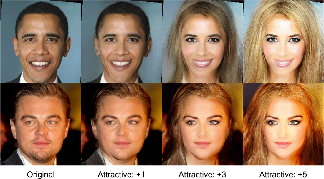
Figure 1: Interpolating along the Attractive latent attribute in different scales converges to pictures of white blonde women.

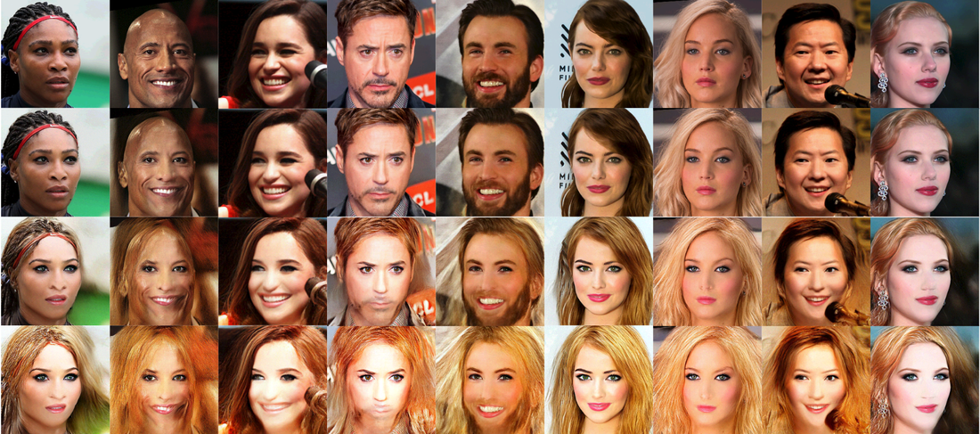
Figure 2: More visualizations of how images of different gender and races converge to young, white-skinned women with long blonde or red hair as we only naively interpolate along the ’attractive’ attribute. From top to bottom: original, attractive: ($\alpha=+1$, attractive: $\alpha=+3$, attractive:$\alpha=+5$.)

As we increase the weight of influence of the attractive-attribute manipulation latent vector, we end up rendering Obama and DiCaprio as almost Caucasian-blonde women. One can attribute this to the possible idiosyncratic co-prevalence of attributes such as blond_Hair, attractive, and pale_Skin in the images of the original dataset.

We acknowledge this troublesome nexus between these three attributes and would like to reiterate that this work does not propose a ‘here’s how you make a face more attractive’ framework but rather focuses on the issue on ignored statistical priors of the (meta)attributes that an image dataset is oft shipped with. Specifically, we address this issue by using graph structured Ising priors to model the inter-attribute statistical dependence and later harnessing this model to propose a corrective procedure that helps allay some of the concerns laid thus far.

The rest of the paper is organized as follows. In Section 2, we cover the estimation procedure for learning the Inter-Attribute Ising Prior (IAIP). In Section 3, we propose our post hoc bias- corrective framework. In Section 4, we showcase some qualitative results that highlights the efficacy of our approach and conclude the paper.

This is a work-in-progress and we have duly open-sourced the implementation along with an interactive portal provides interfaces to both the IAIP as well as the corrective procedure here. This work aims to showcase and correct the bias in the image domain, which draw parallels to the learnt biases in Word2Vec embeddings (Bolukbasi et al., 2016) and other existing study of biases (Torralba et al., )(Tommasi et al., 2017)(Binns, 2017). We’d like to re-emphasize we position this work as a quick-to-implement post-hoc solution and would like to encourage the deep learning community to not just pay attention to the dubious selection-biases in the datasets they use to train their generative models, but to also consider the problem of jointly modeling the attribute space and the pixel-space of images.

2 Learning the Inter-Attribute Ising Prior

Probabilistic graphical models are the unifying framework of choice in areas such as bioinformatics, statistical physics and communication theory for modeling complex dependencies among random variables using ideas from both graph theory and probability theory. This framework not just facilitates building large-scale multivariate statistical models but also allows for elegant visualization and knowledge discovery through the learned statistical dependency graph (Wainwright et al., 2008). In this paper, we choose a specific type of binary Markov Random Fields (MRFs) termed as Ising Models (see (Stanley, 1971)) to model the inter-attribute statistical dependencies. The model specifies a distribution $p(\mathbf{a})$ defined over a substrate graph, $G^{\textrm{(ising)}}(V,E)$. Specifically the conditional distribution of an attribute $a_{j}\in\{0,1\}$ given the rest of the attributes $a_{\backslash j}$ and the graph $G^{\textrm{(ising)}}(V,E)$ takes the form:

$${p_{\Omega}}\left({{a_{j}}|{a_{\backslash j}}}\right)=\frac{{\exp\left[{{\tau_{j}}{a_{j}}+{a_{j}}\sum\limits_{k\in{V_{\backslash j}}}{\left({{\beta_{jk}}{a_{k}}}\right)}}\right]}}{{1+\exp\left[{{\tau_{j}}+\sum\limits_{k\in{V_{\backslash j}}}{\left({{\beta_{jk}}{a_{k}}}\right)}}\right]}}$$ (1)

Here, $\tau_{j}$ and $\beta_{jk}$ are the node parameters and Ising edge parameters respectively.

In order to learn the underlying graph and the associated node and edge weights, we use a network estimation procedure termed eLasso that combines $\ell_{1}$-regularized logistic regression with model selection criterion based on the Extended Bayesian Information Criterion (EBIC).

The EBIC cost function is defined as:

$$\mathit{BIC}_{\gamma}\left({{{\hat{\Omega}}_{j}}}\right)=-2\ell\left({{{\hat{\Omega}}_{j}}}\right)+n_{nei}(\rho)\log\left(N_{\mathit{dataset}}\right)\\ +2\gamma n_{nei}(\rho)\log\left({N_{\mathit{attributes}}-1}\right)$$ (2)

Here, $N_{\mathit{dataset}}$ represents the number of observations (which is 30,000 in the case of Celeb-A-HQ dataset), $N_{\mathit{attributes}}-1$ represents the number of covariates (predictors), $n_{nei}(\rho)$ represents the cardinality of the neighbors set chosen by the logistic regression at a certain penalty weight $\rho$, and $\gamma$ is the prior strength goodness-of-fit hyperparameter (Van Borkulo et al., 2014).

So, given the binary attribute matrix $A\in\{0,1\}^{N_{\mathit{dataset}}\times N_{\mathit{attributes}}}$, the log-likelihood cost function for the $j^{th}$ attribute, $\ell\left({{{\hat{\Omega}}_{j}}}\right)$ is defined as:

$$\ell\left({{{\hat{\Omega}}_{j}}}\right)=\sum\limits_{i=1}^{N_{\mathit{dataset}}}{\left({{\tau_{j}}{A_{ij}}+\sum\limits_{k\in{V_{\backslash j}}}{\left({{\beta_{jk}}{A_{ij}}{A_{ik}}}\right)-\log\left({1+\exp\left\{{{\tau_{j}}+\sum\limits_{k\in{V_{\backslash j}}}{{\beta_{jk}}{A_{ik}}}}\right\}}\right)}}\right)}$$ (3)

After learning the node weights and the edge weights using the IsingFit procedure, we symmetrize the weights as:

$$w_{jk}=\begin{cases}\frac{(\beta_{jk}+\beta_{kj})}{2},&\text{if }\beta_{jk}\neq 0\textit{ and }\beta_{kj}\neq 0\\ 0,&\text{otherwise}\end{cases}$$ (4)

2.1 The learned IAIP for the CelebA-HQ dataset

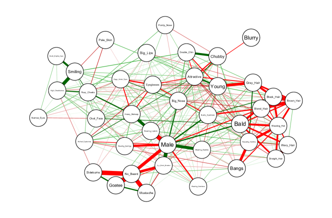
Figure 3: Visualization of Ising model of binary attributes, with green denoting positive edges and red denoting negative edges.

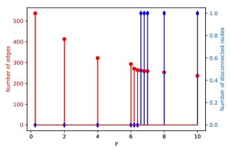
Figure 9: Goodness-of-fit parameter ($\gamma$) selection.

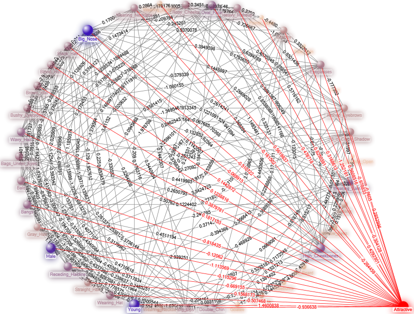
Figure 10: The weighted graph representing the Ising model for the binary attributes of the CelebA-HQ dataset.

As we learn in the following section, we’d ideally want the learned graph $G^{\textrm{(ising)}}(V,E)$ to be connected (no disconnected nodes) as well as sparse. Therefore, we set the the goodness-of-fit parameter ($\gamma$) of the eLasso algorithm to be the largest value above which the resultant graph was disconnected. This variation of the sparsity level of the graph obtained with regards to the number of disconnected nodes as well as the number of edges (a sparsity measure) is seen in Figure 9. As seen, that critical value of the prior strength parameter is $\gamma=6.4$. In Figure 10 and Figure 3, we visualize the weighted graph representing the Ising model learned for the $40$ binary attributes of the CelebA-HQ dataset (with $\gamma=6.4$).

This graph will not just pave the way for the bias corrective procedure to be proposed in the upcoming section, but will also serve as a succinct representation of uncovering anthropocentric bias ingrained during the labeling process itself by the human annotators, by means of Graph exploration using popular GUI Graph visualization software such as Gephi and NodeXL.

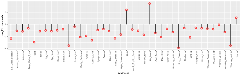
Figure 11: Attribute-wise thresholds (or node parameters $\tau_{i}$) used during the eLASSO fitting procedure

With regards to this eLasso fitting procedure, we have the following figures. In Figure 11, we see the attribute-wise thresholds (or node parameters $\{\tau_{i}\,i\in V\})$. This threshold captures the propensity of a specific attribute to be present in an image in the dataset.

As seen, most of the thresholds (with the exception of Male, No-Beard and Young) are all negative. This implies most of the attributes in the CelebA-HQ dataset in-fact exude a normative disposition to be absent. The attributes Rosy-cheeks, Blurry and Wearing-necktie had the strongest negative thresholds. This implies that these symptoms had the strongest probability of being present in a CelebA-HQ image compared to the other attributes. In Figure 12, we see that variation of the tuning parameter per attribute that was used to ensure the best-fit set of neighbors (see (Van Borkulo et al., 2014)). As seen, the features Mouth-slightly-open and Pointy-nose had the largest values of the tuning parameters associated with them.

3 Methodology

In this section, we denote the notation $\psi\left({}\right):{\mathbf{x}}\to{\mathbf{z}}$ denotes the pixel-space to latent-space encoder and $\phi\left({}\right):{\mathbf{z}}\to{\mathbf{x}}$ denotes the latent-space to pixel-space decoder. We begin by reviewing the current procedure for latent space manipulation and then propose our correction.

3.1 Current procedure for latent space manipulation

The current procedure for latent space interpolation firsts encode inputs and compute the average latent vector of inputs with and without the attribute. The latent space manipulation vectors are

$${{\mathbf{Z}}^{(manip)}}=\left\{{{\mathbf{z}}_{i}^{(manip)}}\right\}_{i=1}^{40}$$ (5)

where for the $i^{th}$ attribute,

$${\mathbf{z}}_{i}^{(manip)}=\frac{{\sum\limits_{t=1}^{{N_{\mathit{dataset}}}}{\psi\left({{{\mathbf{x}}_{t}}\cdot\mathbbm{1}\left[\kern-1.49994pt\left[{{A_{ti}}==+1}\right]\kern-1.49994pt\right]}\right)}}}{{\sum\limits_{t=1}^{{N_{\mathit{dataset}}}}{\mathbbm{1}\left[\kern-1.49994pt\left[{{A_{ti}}==+1}\right]\kern-1.49994pt\right]}}}-\frac{{\sum\limits_{t=1}^{{N_{\mathit{dataset}}}}{\psi\left({{{\mathbf{x}}_{t}}\cdot\mathbbm{1}\left[\kern-1.49994pt\left[{{A_{ti}}==0}\right]\kern-1.49994pt\right]}\right)}}}{{\sum\limits_{t=1}^{{N_{\mathit{dataset}}}}{\mathbbm{1}\left[\kern-1.49994pt\left[{{A_{ti}}==0}\right]\kern-1.49994pt\right]}}}$$ (6)

Here, $A\in\{0,1\}^{N_{\mathit{dataset}}\times N_{\mathit{attributes}}}$ represents the binary attribute matrix for the dataset and $A_{ti}$ represents the binary value for the $i^{th}$ attribute in the $t^{th}$ image out of $N_{\mathit{dataset}}$ images in the dataset. $\mathbbm{1}\left[\kern-1.49994pt\left[{e}\right]\kern-1.49994pt\right]$ represents the identity function

$$\mathbbm{1}\left[\kern-1.49994pt\left[e\right]\kern-1.49994pt\right]=\left\{{\begin{array}[]{*{20}{c}}1,&\text{if e = TRUE}\\ 0,&\text{otherwise.}\end{array}}\right.$$ (7)

After obtaining the latent space manipulation vectors, we can manipulate over the latent space given an input tuple of image, attribute-index and weight of manipulation $(\mathbf{x},i,\alpha)$. By first encoding a raw image $\mathbf{x}$ in latent space as $\psi(\mathbf{x})$, One can interpolate over the latent space by some degree $\alpha$:

$${{\mathbf{z}}^{\left({manip\_orig,i,\alpha}\right)}}=\psi\left({\mathbf{x}}\right)+\alpha{\mathbf{z}}_{i}^{(manip)}$$ (8)

To obtain the manipulated image, the interpolated latent vector is decoded to obtain ${{{\mathbf{z}}^{\left({manip\_orig,i,\alpha}\right)}}}$:

$${{\mathbf{x}}^{\left({manip\_orig,i,\alpha}\right)}}=\phi\left({{{\mathbf{z}}^{\left({manip\_orig,i,\alpha}\right)}}}\right)$$ (9)

3.2 Proposed modified procedure for latent space manipulation

We suggest that we first realign the latent space attribute-wise manipulation vectors by adding a Markov-blanket correction factor to the vectors computed in Eq 6 that takes into account the neighboring attributes (nodes) unearthed in the Ising prior graph learned from the dataset in Section 2. That is, we generate different latent manipulation vectors derived from Equation 5 as

$${{\mathbf{Z}}^{(manip\_mb)}}=\left\{{{\mathbf{z}}_{i}^{(manip\_mb)}}\right\}_{i=1}^{40}$$ (10)

where for the $i^{th}$ attribute,

$${\mathbf{z}}_{i}^{(manip\_mb)}={\mathbf{z}}_{i}^{(manip)}\overbrace{-\mu\sum\limits_{k\in{\mathcal{N}_{i}}\left({G^{\textrm{(ising)}}(V,E)}\right)}{\left({{w_{ik}}{\mathbf{z}}_{k}^{(manip)}}\right)}}^{markov-blanket-correction}.$$ (11)

Here $\mu$ is the Markov-blanket correction strength parameter, ${\mathcal{N}_{i}}$ is the Markov-blanket neighborhood of the $i^{th}$ attribute (node) in the Ising-graph ${G^{\textrm{(ising)}}(V,E)}$ learned in Section 2.

Now, the output images with Markov-blanket corrections, ${{\mathbf{x}}^{\left({manip\_mb,i,\alpha}\right)}}$, are generated by:

$$\begin{gathered}{{\mathbf{z}}^{\left({manip\_mb,i,\alpha}\right)}}=\psi\left({\mathbf{x}}\right)+\alpha\left({{\mathbf{z}}_{i}^{(manip)}\overbrace{-\mu\sum\limits_{k\in{N_{i}}\left({{G^{({\text{ising}})}}(V,E)}\right)}{\left({{w_{ik}}{\mathbf{z}}_{k}^{(manip)}}\right)}}^{markov-blanket-correction={\mathbf{z}}_{i}^{(manip\_mb)}}}\right)\hfill\\ {{\mathbf{x}}^{\left({manip\_mb,i,\alpha}\right)}}=\phi\left({{{\mathbf{z}}^{\left({manip\_mb,i,\alpha}\right)}}}\right)\hfill\\ \end{gathered}$$ (12)

Given the proposed modified method of correctly manipulating across the latent space, we define the full algorithm as per Algorithm 1.

Algorithm 1 Corrective Bias Latent Manipulation Algorithm

  Input: data $\bm{x}$, priors $\bm{A}$, attributes to interpolate $A$, degree of interpolation $\alpha$, hyperparameter $\gamma,\mu\in\mathbb{R}^{+}$

  $G(V,E)\leftarrow$ Ising Graph of ($\bm{A},\gamma$)

  $\psi\leftarrow$ model mapping $\bm{x}$ to $\bm{z}$

  $\phi\leftarrow$ model mapping $\bm{z}$ to $\bm{x}$

  $z_{m}\leftarrow$ manipulation vectors

  Initialize $\bm{z^{\prime}}$ as $\psi(\bm{x})$

  for $\alpha_{i}=\alpha_{1},\alpha_{2},\dots,\alpha_{m}$ in $\bm{\alpha}$ do

     $\bm{z^{\prime}}\leftarrow\bm{z^{\prime}}+\alpha z_{m_{i}}$

     $\mathcal{N}\leftarrow$ neighborhood/adjacent vertices of $z_{m_{i}}$ in $G$

     for $k$ in $\mathcal{N}$ do

        $\bm{z^{\prime}}\leftarrow\bm{z^{\prime}}+-\alpha\cdot\mu\cdot w_{ik}(z_{m_{k}})$

     end for

  end for

  $\bm{\hat{x}}\leftarrow\phi(\bm{z^{\prime}})$, the interpolated image with corrective bias

4 Results and Discussion

In this section, we focus on showcasing the efficacy of our procedure by qualitative methods. Before we dive into the qualitative experiments, we’d like explore if the (Ising) weights of $G^{\textrm{(ising)}}(V,E)$, that is, $\left\{{{w_{ij}}}\right\};\forall(i,j)\in E$ that are indeed correlated with the respective (angular) distance between the latent vectors $\mathbf{z}_{i},\mathbf{z}_{j}$. This would help broadly understand how much of the separation between the latent space representations is on account of mere co-occurrence of the attributes and how much can be attributed to the deep-encoder being able to organically tease out the semantic separation between the attributes.

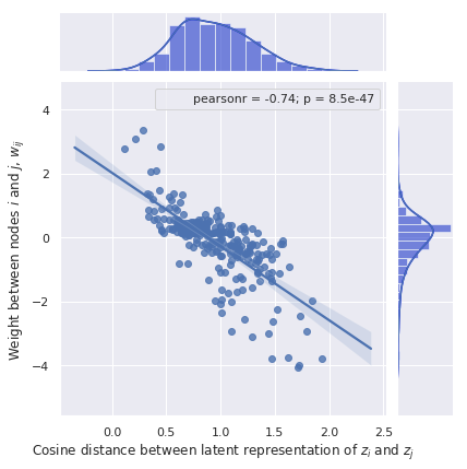
Figure 4: Plot of Ising weights against latent manipulation vectors between the connected nodes in Ising graph.

Figure 4 presents the scatter-plots between the Ising weights $w_{ij}$ and $d_{ij}$ as the cosine distance between $\mathbf{z}_{i}$ and $\mathbf{z}_{j}$, the latent manipulation vectors associated with attribute indices $i$ and $j$.

The strong negative correlation $(R_{\mathit{pearson}}=-0.74;p=8.5e^{-47})$ confirms our hunch that the co-occurrence of attributes has strongly influenced the latent space. That is, two attributes that always co-occurred in the image dataset (meaning high edge-weight $w_{ij}$ in the Ising prior) ended up with latent space representations with a low cosine distance between them. We posit this might be more of a bug than a feature of the model as this alludes towards the notion that coincidental occurrences will strongly influence the semantic distancing in the latent space.

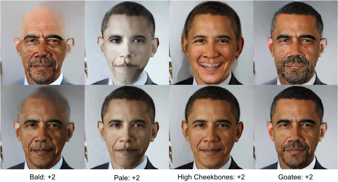
Figure 5: Top: Naively manipulating attribute by +2. Bottom: manipulating attribute by +2 while applying corrective bias penalty to corresponding Markovian blankets.

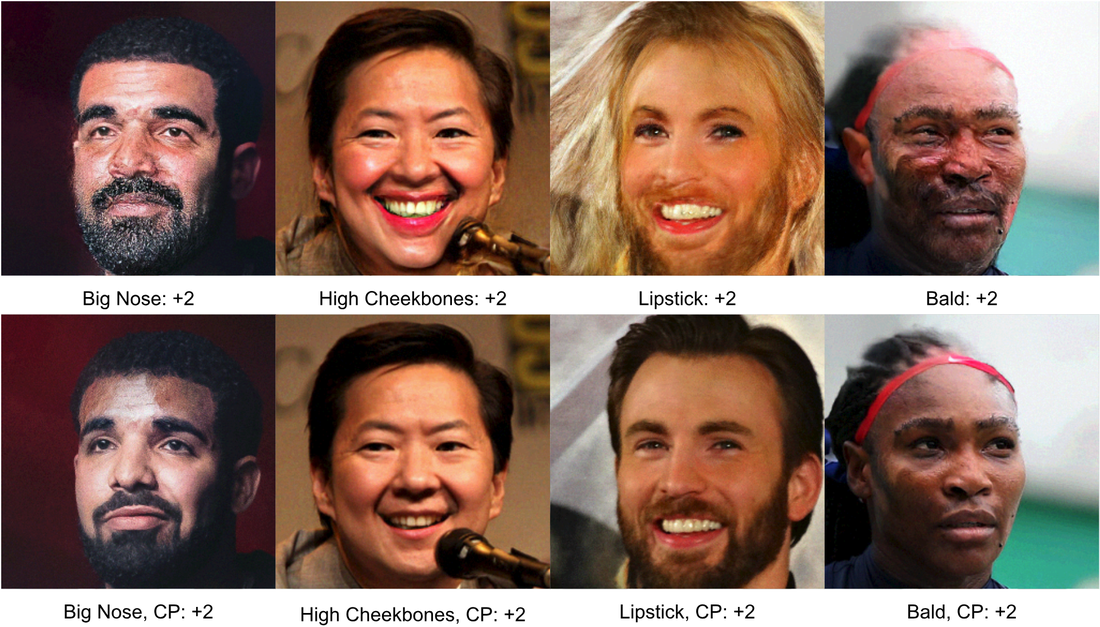
Figure 6: Naive manipulation across one attribute (top) vs manipulation with corrective penalty on neighborhood attributes.

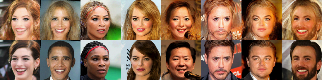
Figure 7: Demonstration on how inherent bias in the ’wearing lipstick’ attribute commonly correlated with blonde hair, young and women can be corrected using our proposed corrective bias algorithm. Top: wearing lipstick: +2. Bottom: wearing lipstick: +2 with neighborhood corrective penalty.

Some attributes are mutually associated with others through stereotypes, which experimentally justifies the need for bias correction. As shown in Figure 6, increasing High_Cheekbones also subtly increases the attributes of Smiling, Female and Wearing_Lipstick which are usually associated with feminine characteristics. On the other hand, increasing attributes such as Bald also shows increases likelihood of Goatee, Chubby and Male. Applying such attributes in images in contrasting domains (increasing Lipstick for male, Bald for females) cause the transformed images to lose intrinsic properties of the original image by generalizing towards the implicitly learnt bias. This is also confirmed in Figure 5, where increasing baldness changes the skin color to be that of a white forehead.

We also demonstrate how biases can be corrected as shown in Figure 7. Using Wearing_Lipstick as an example, which is implicitly associated with feminine characteristics, the image learns to transform with biases such as Blonde_Hair, Female and Wearing_Makeup. However, by accounting for biases, we show how Wearing_Lipstick can be applied across different characteristic domains such as gender and race, while preserving the inherent attributes in the image transformation process.

5 Conclusion

We demonstrate that models that directly learn to model the input data without considering attribute priors while training reveal significant bias. Using Glow as an example of flow-based generative models, we reveal the existing bias by manipulating across the latent space, which mirrors common racial and gender stereotypes.

We also emphasize that this bias also exists in other generative models such as GANs and VAEs as shown in the Appendix. We propose a post-hoc corrective measure for models trained with existing bias by using Ising models fitted on attribute priors.

6 Appendix

6.1 Visializing Learnt Biases in Generative Models

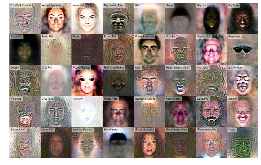
Figure 8: Bias of CelebA illustrated: Visualization of biases in latent space of Generative Adversarial Interpolative Autoencoding (GAIA) (Sainburg et al., 2018). Visualization of latent ‘attractive’, ‘big nose’, and ‘big lips’ correlate to racial profiles that reveal the inherent bias in CelebA.

6.2 Visualization of Ising Graphs

Figure 12: Attribute-wise variation of the tuning parameter ($\lambda$) that was used to achieve the best fit set of neighbors during the Ising prior learning

6.3 Generalizing beyond Normalizing Flows: Revealing Bias in Generative Adversarial Networks Trained on CelebA/CelebA-HQ

We can further confirm that the CelebA dataset is the root cause of the bias shown experimentally by revealing similar biases in other models, such as Generative Adversarial Networks. Below, we experiment with two GAN architectures trained on the CelebA dataset.

Note that the pretrained models only allow the manipulation of 13 attributes: Bald, Bangs, Black_Hair, Blond_Hair, Brown_Hair, Bushy_Eyebrows, Eyeglasses, Male, Mouth_Slightly_Open, Mustache, No_Beard, Pale_Skin, Young.

6.3.1 AttGAN: Facial Attribute Editing by Only Changing What You Want

AttGAN, by He et al., was created specifically to modify attributes realistically and in isolation, so that users can “change what [they] want” (He et al., 2017). Users can choose to modify any number of attributes simultaneously, as well as adjust the magnitude of adjustment per attribute.

The authors of AttGAN understand that attributes in CelebA are highly correlated, claiming that in previous models, “adding blond hair always makes a male become a female because most blond hair objects are female in the training set”. He et al. correct the effects of this correlation by placing constraints on the images generated from latent representations, enforcing these constraints by employing an attribute classifier, a main contribution of their paper.

We begin by observing that adjusting the Male attribute negatively causes the AttGAN model to generate long hair and add makeup. Next, we adjust the Blond_Hair attribute, and observe that this causes the GAN to generate blue eyes and long hair.

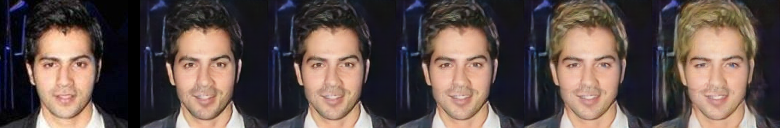
Figure 13: Top: Example of interpolating Male attribute between -2 and +2. Bottom: Example of interpolating Blond_Hair attribute between -2 and +2. Leftmost image is original image.

We also increase the Blond_Hair attribute and the Male attributes together. One might expect increasing the Male attribute to counteract the long-hair that the Blond_Hair attribute creates. However, as we can see below, it on occasion acts constructively. It is clear that, even with the addition of an attribute classifier to constrain the model, the latent representation manipulations for separate attributes are still not independent. We note, though, that this behavior is seen mostly when the original images are of males. He et al. themselves conclude that model errors occur mostly when large modifications are made to images, such as adding hair to a bald figure.

Lastly, we investigate the manipulation of facial hair. It seems that mustaches and beards are always generated black regardless of the original subject’s hair color. In fact, if we attempt to generate a mustache on top of a subject who already has facial hair, it simply changes the color of the existing facial hair to black. Additionally, if we generate a mustache on top of a young or less masculine subject, the rest of the face is morphed into that of a more elderly and rugged man.

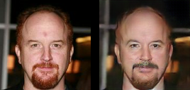
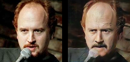
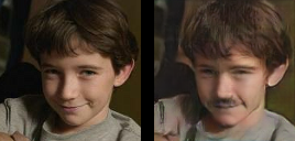
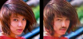
Figure 14: Top: Examples of manipulating both Male and Blond_Hair attributes by +1. Middle: Manipulating Mustache attribute by +1 on a subject with existing facial hair. Bottom: Manipulating Mustache attribute by +1 on a young subject with less masculine features.

6.3.2 STGAN: A Unified Selective Transfer Network for Arbitrary Image Attribute Editing

We also carry out experiments on STGAN, a model built by Liu et al. (Liu et al., 2019) extending He et al.’s work. Their main contribution is the selectivity of information passed into their model’s generators, choosing only to pass in the difference in attribute vector between the source and target image, so that the generator supposedly only affects the targeted change in attribute.

As with AttGAN, we begin by manipulating the Male attribute. We can see that STGAN is less inclined to generate longer hair when decreasing this attribute, but it generates black splotches in the shape of hair, simply without the texture and details of hair. It is obvious that STGAN still suffers from the safe bias in the priors as other models.

Like AttGAN, STGAN changes the eye color of its subject towards blue when increasing the Blond_Hair attribute. However, it does not generate long hair like AttGAN does.

Figure 15: Top: Example of interpolating Male attribute between -2 and +2. Bottom: Example of interpolating Blond_Hair attribute between -2 and +2. Leftmost image is original image.

Increasing the Blond_Hair and the Male attributes together reproduces the constructive interaction seen in AttGAN, where even more blond long hair is generated than increasing just Blond_Hair on its own. This underlying complex interaction in the latent space seems to be a consistent problem across generative models, as far as we can tell.

Like AttGAN, generated facial hair is always black, regardless of the original subject’s hair color, generating a mustache on top of a subject who already has facial hair simply darkens the color of the existing facial hair, and generating a mustache on a young/soft-featured subject makes them appear older and more masculine.

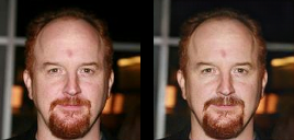
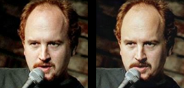
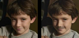
Figure 16: Top: Examples of manipulating both Male and Blond_Hair attributes by +1. Middle: Manipulating Mustache attribute by +1 on a subject with existing facial hair. Bottom: Manipulating Mustache attribute by +1 on a young subject with less masculine features.

6.3.3 DNA-GAN: Learning Disentangled Representations from Multi-Attribute Images

Figure 17: Interpolating on ‘wearing eyeglasses’ changes the racial profile of the subject matter for DNA-GAN.

DNA-GAN is a supervised method for disentangling multiple factors of variation simultaneously by using multi-attribute images (Xiao et al., 2018). Trained on CelebA, it can manipulate several attributes in the latent representations of images, which is a generalization of GeneGAN (Zhou et al., 2017). DNA-GAN replaces the explicit nulling loss with the annihilating operation and employs a single discriminator for guiding images generation on multiple attributes.

While it seeks to disentangle multiple factors and attributes of images, we see the inherent bias reflected in the CelebA dataset as per Figure 17. While we manipulate across the ‘wearing eyeglasses’, the racial profile of the subject matter being manipulated also changes accordingly.

6.3.4 Generative Adversarial Interpolative Autoencoding (GAIA)

The Generative Adversarial Interpolative Autoencoder (GAIA) is novel hybrid between the Generative Adversarial Network (GAN) and the Autoencoder (AE) (Sainburg et al., 2018). It addresses the issue of GANs which are non-bidirectional, while also addressing issues of autoencoders which produces blurry images, and addressing the non-conves latent spaces of autoencoders.

GAIA promotes a convex latent distribution by training adversarially on latent space interpolations. Trained on CelebA, GAIA produces non-blurry samples that match both high- and low-level features of the original images. Upon visualizing the inherent latent spaces learnt, we see that attributes such as ‘big nose’ and ‘big lips’ correlate to racial profiles that reveal the inherent bias in CelebA, as per Figure 8.

References

- (1) Barocas, S., Hardt, M., and Narayanan, A. Fairness and machine learning. fairmlbook. org, 2018. URL: http://www. fairmlbook. org.
- Binns (2017) Binns, R. Fairness in machine learning: Lessons from political philosophy. arXiv preprint arXiv:1712.03586, 2017.
- Bolukbasi et al. (2016) Bolukbasi, T., Chang, K.-W., Zou, J. Y., Saligrama, V., and Kalai, A. T. Man is to computer programmer as woman is to homemaker? debiasing word embeddings. In Advances in neural information processing systems, pp. 4349–4357, 2016.
- Dinh et al. (2014) Dinh, L., Krueger, D., and Bengio, Y. Nice: Non-linear independent components estimation. arXiv preprint arXiv:1410.8516, 2014.
- Goodfellow et al. (2014) Goodfellow, I., Pouget-Abadie, J., Mirza, M., Xu, B., Warde-Farley, D., Ozair, S., Courville, A., and Bengio, Y. Generative adversarial nets. In Advances in neural information processing systems, pp. 2672–2680, 2014.
- He et al. (2017) He, Z., Zuo, W., Kan, M., Shan, S., and Chen, X. Arbitrary facial attribute editing: Only change what you want. CoRR, abs/1711.10678, 2017. URL http://arxiv.org/abs/1711.10678.
- Karras et al. (2017) Karras, T., Aila, T., Laine, S., and Lehtinen, J. Progressive growing of gans for improved quality, stability, and variation. arXiv preprint arXiv:1710.10196, 2017.
- Kingma & Dhariwal (2018) Kingma, D. P. and Dhariwal, P. Glow: Generative flow with invertible 1x1 convolutions. In Advances in Neural Information Processing Systems, pp. 10215–10224, 2018.
- Kingma & Welling (2013) Kingma, D. P. and Welling, M. Auto-encoding variational bayes. arXiv preprint arXiv:1312.6114, 2013.
- Liu et al. (2019) Liu, M., Ding, Y., Xia, M., Liu, X., Ding, E., Zuo, W., and Wen, S. Stgan: A unified selective transfer network for arbitrary image attribute editing. 2019.
- Liu et al. (2015) Liu, Z., Luo, P., Wang, X., and Tang, X. Deep learning face attributes in the wild. In Proceedings of International Conference on Computer Vision (ICCV), 2015.
- Sainburg et al. (2018) Sainburg, T., Thielk, M., Theilman, B., Migliori, B., and Gentner, T. Generative adversarial interpolative autoencoding: adversarial training on latent space interpolations encourage convex latent distributions. arXiv preprint arXiv:1807.06650, 2018.
- Stanley (1971) Stanley, H. E. Phase transitions and critical phenomena. Clarendon Press, Oxford, 1971.
- Tom Yeh et al. (2017) Tom Yeh, M. et al. Designing a moral compass for the future of computer vision using speculative analysis. In Proceedings of the IEEE Conference on Computer Vision and Pattern Recognition Workshops, pp. 64–73, 2017.
- Tommasi et al. (2017) Tommasi, T., Patricia, N., Caputo, B., and Tuytelaars, T. A deeper look at dataset bias. In Domain adaptation in computer vision applications, pp. 37–55. Springer, 2017.
- (16) Torralba, A., Efros, A. A., et al. Unbiased look at dataset bias. Citeseer.
- Van Borkulo et al. (2014) Van Borkulo, C. D., Borsboom, D., Epskamp, S., Blanken, T. F., Boschloo, L., Schoevers, R. A., and Waldorp, L. J. A new method for constructing networks from binary data. Scientific reports, 4:5918, 2014.
- Wainwright et al. (2008) Wainwright, M. J., Jordan, M. I., et al. Graphical models, exponential families, and variational inference. Foundations and Trends® in Machine Learning, 1(1–2):1–305, 2008.
- Xiao et al. (2018) Xiao, T., Hong, J., and Ma, J. Dna-gan: Learning disentangled representations from multi-attribute images. International Conference on Learning Representations, Workshop, 2018.
- Zhou et al. (2017) Zhou, S., Xiao, T., Yang, Y., Feng, D., He, Q., and He, W. Genegan: Learning object transfiguration and attribute subspace from unpaired data. arXiv preprint arXiv:1705.04932, 2017.