On the estimation of average treatment effects with right-censored time to event outcome and competing risks

On the estimation of average treatment effects with right-censored time to event outcome and competing risks

Abstract

We are interested in the estimation of average treatment effects based on right-censored data of an observational study. We focus on causal inference of differences between t-year absolute event risks in a situation with competing risks. We derive doubly robust estimation equations and implement estimators for the nuisance parameters based on working regression models for the outcome, the censoring and the treatment distribution conditional on auxiliary baseline covariates. We use the functional delta method to show that our estimators are regular asymptotically linear estimators and estimate their variances based on estimates of their influence functions. In empirical studies we assess the robustness of the estimators and the coverage of confidence intervals. The methods are further illustrated using data from a Danish registry study.

1 Introduction

Average treatment effects (ATE) are important parameters in epidemiology (Robins, 1986; Hernán and Robins, 2006). In observational studies, these parameters are interpreted in a suitable framework for causal inference (Hernán and Robins, 2019; Pearl, 2000) as what one would have observed had the treatment been randomized. Estimators of average treatment effects include outcome regression model based estimators which standardize the expected outcome to a given distribution of the confounders (G-formula), inverse probability of treatment weighted (IPTW) estimators which rely on a model for the propensity of treatment, and doubly robust estimators which combine the two types of estimators with the aim to reduce bias (van der Laan and Robins, 2003; Kang et al., 2007; Glynn and Quinn, 2010).

In this article, we are motivated by applications in pharmacoepidemiology where the aim is to evaluate differences between alternative drug treatments based on large scale registry data (Hernán and Robins, 2016). We are particularly interested in applications where the outcome is a right censored time to event and death without the outcome is a competing risk. We restrict our discussion to the simple setting where a treatment decision is made only once at baseline and all patients are supposed to stay on treatment for a pre-specified amount of time, say until $\tau$-years after initiation of the treatment. We then consider treatment differences between the absolute $\tau$-year risks of an event of interest as the main target parameter and aim to achieve an interpretation in the counterfactual world where the treatment is randomized.

Compared to other approaches for competing risk data (Andersen et al., 2017; Bekaert et al., 2010; Moodie et al., 2014), the major difference of our approach is that we use working Cox regression models for the cause-specific hazard rates to estimate the absolute risk of the event (Benichou and Gail, 1990; Ozenne et al., 2017). Furthermore, we allow the censoring distribution to depend on baseline covariates via a separate Cox regression model and work with a logistic regression model for the propensity of treatment. We study the robustness of our estimator to a possible misspecification of any of these working models. Our work relates and extends recent developments in survival analysis: Wang et al. (2016) proposed a doubly robust estimator for right-censored survival data when using parametric working regression models for the outcome distribution and the treatment distribution, and a non-parametric model (Kaplan Meier) for the censoring distribution. Using the semiparametric theory (Bickel et al., 1993; van der Laan and Robins, 2003; Tsiatis, 2006), we derive an augmentation term which makes our estimator robust against misspecification of the censoring model. The augmentation term resembles the one in the survival case (Zhao et al., 2014). We also derive the influence function of our estimator and show that it can be greatly simplified when all working models are correctly specified.

This paper is structured as follows: Section 2 formally introduces the competing risk setting, the parameter of interest, and the statistical models. Section 3 presents the G-formula, IPTW, and doubly robust estimators in a competing risk setting. We derive in section 4 the asymptotic properties of our three estimators: consistency, asymptotic normality, and their influence function. Robustness of the estimators to model misspecification and coverage of confidence intervals based on the asymptotic distribution of the estimators is assessed in section 5 using simulation studies. Finally, in section 6, we apply our estimators to compare two anticoagulation treatments regarding their impact on the risk of bleeding (adverse endpoint) in patients with atrial fibrillation. The data used for this illustration are a subset of the data of Stærk et al. (2018), where we applied Cox regression for the event hazard and the hazard of death without event in order to estimate average differences in $\tau$-year risk of stroke and bleeding between alternative drugs for anticoagulation therapy.

2 Competing risk setting

2.1 Notation and parameter of interest

We consider a random sample of $n$ individuals $\{(\tilde{T}_{i},\tilde{\Delta}_{i},A_{i},W_{i})\}_{i=1}^{n}$ where $A$ is a binary treatment variable assigned at baseline, $W$ a $d$-dimensional vector of auxiliary covariates measured at baseline, $\tilde{T}$ a right-censored event time, i.e., $\tilde{T}=T\wedge C$ where $T$ is the event time, $C$ the censoring time, $\Delta$ is the event type for which we assume that $\{\Delta=1\}$ means that the event of interest occurred and $\{\Delta=2\}$ that the competing event occurred, and $\tilde{\Delta}=\Delta\mathrm{1}{\{T\leq C\}}$ indicates uncensored observation (we use $\mathrm{1}{\{\cdot\}}$ to denote the indicator function). We assume throughout that $(T,\Delta)$ are conditionally independent of $C$ given $(W,A)$ and that in the case of tied event and censoring times, i.e., $C=T$, the event time is earlier. Also, for a fixed time point $\tau$ we assume that the probability of right-censoring is bounded away from zero: $\mathrm{P}[C>\tau|A,W]>\epsilon$ where $\epsilon>0$. We denote $Y(\tau)=\mathrm{1}{\{T\leq\tau,\Delta=1\}}$ for the indicator for the event of interest at time $\tau$ and note that its expected value is the absolute risk that the event of interest occurs before time $\tau$.

To define our target parameter we introduce the potential outcomes $Y^{a}(\tau)$, i.e., the response of a randomly selected individual had that individual, possibly contrary to the fact, been given treatment $A=a$. Our target parameter is the expected difference:

$$\Psi(\tau)=\mathrm{E}[Y^{1}(\tau)-Y^{0}(\tau)].$$

We make the following assumptions: $Y(\tau)=(1-A)Y^{0}(\tau)+AY^{1}(\tau)$ (consistency assumption), $\forall a\in\{0,1\}$, $(Y^{a}(\tau),A)$ are conditionally independent given $W$, (no unmeasured confounders), and $\forall(a,w)\in\{0,1\}\times\mathcal{W},\;\mathrm{P}[A=a|w]>0$ (positivity assumption) where $\mathcal{W}\subset R^{d}$ denotes the set of possible values for $W$.

2.2 Modeling

To estimate the target parameter based on the observed data we consider the following conditional distributions as nuisance parameters. The cumulative incidence function $F_{1}$ describes the absolute risk of the event of interest by time $t$:

$$F_{1}(t|A,W) =\mathrm{P}(T\leq t,\Delta=1|A,W),$$

$$G$$ is the conditional probability of being uncensored

$$G(t|A,W) =\mathrm{P}(C>t|A,W),$$

and $$\pi W$$ describes the propensity of treatment conditional on

$$\pi(W) =\mathrm{P}(A=1|W).$$

Under the identifiability assumptions stated in section 2.1 the likelihood of the observed variables $O_{i}=(\tilde{T}_{i},\tilde{\Delta}_{i},A_{i},W_{i})$ factorizes (Begun et al., 1983; Gill et al., 1995) and the density of their joint probability distribution $P$ with respect to a suitable dominating measure can be parametrized

$$\mathrm{P}(\mathrm{d}t,\delta,a,dw)=\{G(t-|a,w)F_{1}(\mathrm{d}t|a,w)(a\pi(w)+(1-a)(1-\pi(w))H(\mathrm{d}w)\}^{\mathrm{1}{\{\delta=1\}}}\\ \{G(t-|a,w)F_{2}(\mathrm{d}t|a,w)(a\pi(w)+(1-a)(1-\pi(w))H(\mathrm{d}w)\}^{\mathrm{1}{\{\delta=2\}}}\\ \{S(t-|a,w)G(\mathrm{d}t|a,w)(a\pi(w)+(1-a)(1-\pi(w))H(\mathrm{d}w)\}^{\mathrm{1}{\{\delta=0\}}}$$

where $F_{2}(t|A,W)=\mathrm{P}(T\leq t,\Delta=2|A,W)$, $H$ is the marginal distribution of $W$, and $t-$ denotes the left-handed limit at time $t$. Our working model for the joint probability distribution $P$ leaves the $H$ part completely non-parametric but for each of the other nuisance parameters we specify a (semi-)parametric regression model as our working model and define a corresponding estimator. Our working model for $F_{1}$ uses the parameterization of Benichou and Gail (1990) in terms of the cumulative cause-specific hazard functions $\Lambda_{1}$ for the event of interest and $\Lambda_{2}$ for the competing event:

$$F_{1}(t|A,W)=\int_{0}^{t}S(s-|A,W)\Lambda_{1}(\mathrm{d}s|A,W)$$ (1)

where $S(s|A,W)=\exp\left\{-(\Lambda_{1}(s|A,W)+\Lambda_{2}(s|A,W))\right\}$ is the event free survival function. Specifically we consider two separate Cox regression models for $\Lambda_{1}$ and $\Lambda_{2}$ such that the model is parameterized in terms of the cause-specific hazard ratios and baseline hazard functions. An alternative parameterization of $F_{1}$ can be obtained by binomial regression for competing risks (Scheike et al., 2008) where the Fine-Gray regression model (Fine and Gray, 1999) is a special case. Our working models for the censoring mechanism and the propensity of treatment are a Cox regression model and a logistic regression model, respectively. Note that all these working models come with their regular asymptotically linear estimators for the respective nuisance parameter based on the observed data. Thus, we assume that there exist regular asymptotically linear estimators $\hat{F}_{1n},\hat{\pi}_{n},\hat{S}_{n},\hat{G}_{n}$ with respective large sample limits $F_{1}^{*},\pi^{*},S^{*},G^{*}$ such that:

$$\begin{split}\sqrt{n}(\hat{\pi}_{n}-\pi^{*})&=\frac{1}{\sqrt{n}}\sum_{i=1}^{n}\mathrm{IF_{\pi^{*}}}(O_{i})+o_{p}(1),\\ \sqrt{n}(\hat{G}_{n}-G^{*})&=\frac{1}{\sqrt{n}}\sum_{i=1}^{n}\mathrm{IF_{G^{*}}}(O_{i})+o_{p}(1),\\ \sqrt{n}(\hat{F}_{1n}-F_{1}^{*})&=\frac{1}{\sqrt{n}}\sum_{i=1}^{n}\mathrm{IF_{F_{1}^{*}}}(O_{i})+o_{p}(1),\\ \sqrt{n}(\hat{S}_{n}-S^{*})&=\frac{1}{\sqrt{n}}\sum_{i=1}^{n}\mathrm{IF_{S^{*}}}(O_{i})+o_{p}(1),\end{split}$$ (2)

where $O_{i}=(\tilde{T}_{i},\tilde{\Delta}_{i},A_{i},W_{i})$ and $\mathrm{IF_{F_{1}^{*}}},\mathrm{IF_{\pi^{*}}},\mathrm{IF_{S^{*}}},\mathrm{IF_{G^{*}}}$ are the influence functions corresponding to the estimators that represent the first order von Mises expansion of the corresponding statistical functional (van der Vaart, 1998). If our working model for $F_{1}$ is correctly specified then the asymptotic bias is zero, $F_{1}^{*}-F_{1}=0$, and the same holds for the working models for $\pi$, $S$ and $G$. Note that since both $F_{1}$ and $S$ can be expressed as differentiable functionals of $\Lambda_{j}$ for $j=1,2$, a sufficient condition for the last two lines of equation (2) is

$$\sqrt{n}(\Lambda_{j}-\Lambda_{j}^{*})=\frac{1}{\sqrt{n}}\sum_{i=1}^{n}\mathrm{IF}_{\Lambda_{j}^{*}}(O_{i})+o_{p}(1),$$

where $\mathrm{IF}_{\Lambda_{j}^{*}}$ is the influence function of the Cox regression estimator of the cumulative hazard function $j$ and $\Lambda_{j}^{*}$ is the corresponding large sample limit.

In case of a misspecified model, an asymptotic linear expansions of the estimators as in equation (2) still continues to hold under the usual regularity conditions around the least-false parameters $F_{1}^{*},\pi^{*},S^{*},G^{*}$ (White, 1982; Hjort, 1992; Bickel et al., 1993; Gerds and Schumacher, 2001). However, there would be a large sample bias.

3 Estimators for the average treatment effect (ATE)

We consider three types of estimators for our estimand $\Psi(\tau)$. Each type is based on a different combination of the outcome model, the treatment model, and the censoring model. We start by defining our estimators in the case without censoring.

3.1 Uncensored data

The first class of estimators is based on the G-causal parameter (Robins (1986), p.1410), also called backdoor adjustment (Pearl (2000), section 3.2), which yields the G-formula:

$$\Psi(\tau)=\mathrm{E}[F_{1}(\tau|A=1,W))-F_{1}(\tau|A=0,W)].$$

Our regression estimator is obtained by substituting $\hat{F}_{1n}$ for $F_{1}$:

$$\widehat{\Psi}_{\text{G-formula}}(\tau)=\frac{1}{n}\sum_{i=1}^{n}\left(\hat{F}_{1n}(\tau|A=1,W_{i})-\hat{F}_{1n}(\tau|A=0,W_{i})\right).$$ (3)

The second class of estimators uses inverse probability-of-treatment weights ($\operatorname{IPTW})$ and is based on the formula:

$$\Psi(\tau)=\mathrm{E}\left[Y(\tau)\left(\frac{A}{\pi(W)}-\frac{1-A}{1-\pi(W)}\right)\right].$$

Our $\operatorname{IPTW}$ estimator is obtained by substituting $\hat{\pi}_{n}$ for $\pi$:

$$\widehat{\Psi}_{\operatorname{IPTW}}(\tau)=\frac{1}{n}\sum_{i=1}^{n}\left(Y_{i}(\tau)\left(\frac{A_{i}}{\hat{\pi}_{n}(W_{i})}-\frac{1-A_{i}}{1-\hat{\pi}_{n}(W_{i})}\right)\right).$$ (4)

The third class of estimators combines the G-formula estimator and the IPTW estimator into a doubly robust estimator (Hernán and Robins, 2019). Following Tsiatis (2006) (section 13.5) we use the formula

$$\Psi(\tau) =\mathrm{E}\left[\frac{Y(\tau)A}{\pi(W)}+F_{1}(\tau|A=1,W)\left(1-\frac{A}{\pi(W)}\right)\right.$$

$$\left.\qquad-\frac{Y(\tau)(1-A)}{1-\pi(W)}-F_{1}(\tau|A=0,W)\left(1-\frac{1-A}{1-\pi(W)}\right)\right].$$

Our augmented $\operatorname{IPTW}$ estimator (denoted $\operatorname{AIPTW}$) substitutes $\hat{\pi}_{n}$ for $\pi$ and $\hat{F}_{1n}$ for $F_{1}$:

$$\widehat{\Psi}_{\operatorname{AIPTW}}(\tau)= \frac{1}{n}\sum_{i=1}^{n}\frac{Y_{i}(\tau)A_{i}}{\hat{\pi}_{n}(W_{i})}+\hat{F}_{1n}(\tau|A=1,W_{i})\left(1-\frac{A_{i}}{\hat{\pi}_{n}(W_{i})}\right)$$

$$\qquad-\frac{Y_{i}(\tau)(1-A_{i})}{1-\hat{\pi}_{n}(W_{i})}-\hat{F}_{1n}(\tau|A=0,W_{i})\left(1-\frac{1-A_{i}}{1-\hat{\pi}_{n}(W_{i})}\right).$$ (5)

We refer to Glynn and Quinn (2010) and Kennedy (2016) for nice reviews of the doubly robust $\operatorname{AIPTW}$ estimator in uncensored data.

3.2 Right-censored data

In presence of right-censoring, the binary outcome at the time point of interest $Y(\tau)$ is not observed for all subjects, it is only observed in the event $\{C>T\wedge\tau\}=\{\tilde{T}>\tau\}\cup\{\tilde{T}\leq\tau,\tilde{\Delta}\neq 0\}$. To construct estimators of the average treatment effect based on the right-censored data, we combine the estimators of the previous section with inverse probability-of-censoring weighting ($\operatorname{IPCW}$) now also using our estimator $\hat{G}_{n}$. Note that the G-formula estimator defined in equation (3) does not explicitly involve $Y(\tau)$ and hence can be applied directly in right-censored data because the outcome model takes care of the censored data. Using that $\mathrm{1}{\{\tilde{T}>\tau\}}Y(\tau)=0$, we define the following $\operatorname{IPCW}$ estimators:

$$\widehat{\Psi}_{\operatorname{IPTW},\operatorname{IPCW}}(\tau)=\frac{1}{n}\sum_{i=1}^{n}\frac{\mathrm{1}{\{\tilde{T}_{i}\leq\tau,\tilde{\Delta}_{i}\neq 0\}}}{\hat{G}_{n}(\tilde{T}_{i}|A_{i},W_{i})}Y_{i}(\tau)\left(\frac{A_{i}}{\hat{\pi}_{n}(W_{i})}-\frac{1-A_{i}}{1-\hat{\pi}_{n}(W_{i})}\right)$$ (6)

$$\widehat{\Psi}_{\operatorname{AIPTW},\operatorname{IPCW}}(\tau)=\frac{1}{n}\sum_{i=1}^{n}\frac{\mathrm{1}{\{\tilde{T}_{i}\leq\tau,\tilde{\Delta}_{i}\neq 0\}}}{\hat{G}_{n}(\tilde{T}_{i}|A_{i},W_{i})}\frac{Y_{i}(\tau)A_{i}}{\hat{\pi}_{n}(W_{i})}+\hat{F}_{1n}(\tau|A=1,W_{i})\left(1-\frac{A_{i}}{\hat{\pi}_{n}(W_{i})}\right)$$

$$\qquad\qquad-\frac{\mathrm{1}{\{\tilde{T}_{i}\leq\tau,\tilde{\Delta}_{i}\neq 0\}}}{\hat{G}_{n}(\tilde{T}_{i}|A_{i},W_{i})}\frac{Y_{i}(\tau)(1-A_{i})}{1-\hat{\pi}_{n}(W_{i})}-\hat{F}_{1n}(\tau|A=0,W_{i})\left(1-\frac{1-A_{i}}{1-\hat{\pi}_{n}(W_{i})}\right).$$ (7)

Both estimators can now be augmented using semi-parametric theory (see van der Laan and Robins (2003)). In appendix A, we derive the set of observed-data estimating functions for $\Psi$. These estimating equations include an augmentation term which, when set to 0, leads to the $\operatorname{IPCW}$ estimators (equations (6) and (7)). Alternatively the augmentation term can be chosen in order to minimize the asymptotic variance of the corresponding estimator. This choice lead to the following estimators (see appendix A for details):

$$\widehat{\Psi}_{\operatorname{IPTW},\operatorname{AIPCW}}(\tau)=\widehat{\Psi}_{\operatorname{IPTW},\operatorname{IPCW}}(\tau)+\frac{1}{n}\sum_{i=1}^{n}\hat{I}(\tilde{T}_{i},\tau|A_{i},W_{i})\left(\frac{A_{i}}{\hat{\pi}_{n}(W_{i})}-\frac{1-A_{i}}{1-\hat{\pi}_{n}(W_{i})}\right)$$ (8)

$$\widehat{\Psi}_{\operatorname{AIPTW},\operatorname{AIPCW}}(\tau)=\widehat{\Psi}_{\operatorname{AIPTW},\operatorname{IPCW}}(\tau)+\frac{1}{n}\sum_{i=1}^{n}\hat{I}(\tilde{T}_{i},\tau|A_{i},W_{i})\left(\frac{A_{i}}{\hat{\pi}_{n}(W_{i})}-\frac{1-A_{i}}{1-\hat{\pi}_{n}(W_{i})}\right)$$ (9)

$$\text{where }\hat{I}(\tilde{T}_{i},\tau|A_{i},W_{i})=\int_{0}^{\tilde{T}_{i}\wedge\tau}\frac{\hat{F}_{1n}(\tau|A_{i},W_{i})-\hat{F}_{1n}(t|A_{i},W_{i})}{\hat{S}_{n}(t|A_{i},W_{i})}\frac{1}{\hat{G}_{n}(t|A_{i},W_{i})}d\hat{M}_{i}^{C}(t).$$

Here $N_{i}^{C}(t)=\mathrm{1}{\{\tilde{T}_{i}\leq t,\tilde{\Delta}_{i}=0\}}$ denotes the censoring counting process of subject $i$ and $\Lambda^{C}$ the cumulative hazard function of $G$ such that $M_{i}^{C}(t)=N_{i}^{C}(t)-\int_{0}^{t}\mathrm{1}{\{\tilde{T}_{i}\geq s\}}\Lambda^{C}(\mathrm{d}s|A_{i},W_{i})$ is a 0 mean process (a martingale with respect ot the natural filtration, see for example Andersen et al., 1993, section II.4). We use the notation $\hat{M}_{i}^{C}(t)=N_{i}^{C}(t)-\int_{0}^{t}\mathrm{1}{\{\tilde{T}_{i}\geq s\}}\hat{\Lambda}^{C}(\mathrm{d}s|A_{i},W_{i})$ and $M_{i}^{C,*}(t)=N_{i}^{C}(t)-\int_{0}^{t}\mathrm{1}{\{\tilde{T}_{i}\geq s\}}\Lambda^{C,*}(\mathrm{d}s|A_{i},W_{i})$ where $\Lambda^{C,*}$ is the large sample limit of $\hat{\Lambda}^{C}$.

4 Asymptotic properties

In this section, we study the asymptotic properties of the following estimators: $\widehat{\Psi}_{\text{G-formula}}(\tau)$, $\widehat{\Psi}_{\operatorname{IPTW},\operatorname{IPCW}}(\tau)$, and $\widehat{\Psi}_{\operatorname{AIPTW},\operatorname{AIPCW}}(\tau)$.

4.1 Consistency

By equation (2) and the law of large numbers we have

$$\lim_{n\to\infty}\widehat{\Psi}_{\text{G-formula}}(\tau)=\mathrm{E}[F_{1}^{*}(\tau|A=1,W))-F_{1}^{*}(\tau|A=0,W)].$$

Thus, if the outcome model is correctly specified at $\tau$, i.e., for $a\in\{0,1\}$ and almost all $w$ $F_{1}(\tau|a,w)=F_{1}^{*}(\tau|a,w)$, then $\widehat{\Psi}_{\text{G-formula}}$ is a consistent estimator for $\Psi(\tau)$. Similarly, we have under the assumptions of Section 2

$$\lim_{n\to\infty}\widehat{\Psi}_{\operatorname{IPTW},\operatorname{IPCW}}(\tau)=\mathrm{E}\Big{[}\frac{G(\tilde{T}|A,W)}{G^{*}(\tilde{T}|A,W)}\Big{\{}\frac{F_{1}(\tau|A=1,W)\pi(W)}{\pi^{*}(W)}.\\ -\frac{F_{1}(\tau|A=0,W)(1-\pi(W))}{1-\pi^{*}(W)}\Big{\}}\Big{]}$$

Hence, if the working models for the treatment and the censoring mechanism are correctly specified, i.e., $\pi(w)=\pi^{*}(w)$ and $G(s|a,w)=G^{*}(s|a,w)$ for all $s\in[0,\tau]$, $a\in\{0,1\}$ and almost all $w$, then $\widehat{\Psi}_{\operatorname{IPTW},\operatorname{IPCW}}(\tau)$ is consistent. The following theorem states sufficient conditions under which $\widehat{\Psi}_{\operatorname{AIPTW},\operatorname{AIPCW}}$ is consistent.

Theorem 1

Under the assumptions stated in Section 2, the estimator $\widehat{\Psi}_{\operatorname{AIPTW},\operatorname{AIPCW}}(\tau)$ is consistent whenever one of the following conditions is satisfied for all $s\in[0,\tau]$, $a\in\{0,1\}$ and almost all $w$:

1. $G^{*}(s|a,w)=G(s|a,w)$ and $F_{1}^{*}(\tau|a,w)=F_{1}(\tau,a,w)$

2. $G^{*}(s|a,w)=G(s|a,w)$ and $\pi^{*}(w)=\pi(w)$

3. $F_{1}^{*}(s|a,w)=F_{1}(s|a,w)$ and $S^{*}(s|a,w)=S(s|a,w)$

Proof: Roughly, when the censoring model is correctly specified, 1. and 2. follow from the fact that $\widehat{\Psi}_{\operatorname{AIPTW},\operatorname{AIPCW}}(\tau)$ and $\widehat{\Psi}_{\operatorname{AIPTW}}(\tau)$ have the same large sample limit. When the censoring model is misspecified but the outcome and survival models are correctly specified then $\widehat{\Psi}_{\operatorname{AIPTW},\operatorname{AIPCW}}(\tau)$ and $\widehat{\Psi}_{\text{G-formula}}(\tau)$ have the same large sample limit, which gives 3. Appendix B provides the details.

4.2 Asymptotic distribution

All estimators described in the previous section can be written as averages of the estimated nuisance parameters:

$$\widehat{\Psi}_{x}(\tau)= \frac{1}{n}\sum_{i=1}^{n}h_{x}(\tau;O_{i};\hat{F}_{1n},\hat{\pi}_{n},\hat{S}_{n},\hat{G}_{n})$$

$$\text{where }x\in \{{\scriptsize\text{G-formula}};{\scriptsize\text{IPTW,IPCW}};{\scriptsize\text{AIPTW,IPCW}};{\scriptsize\text{IPTW,AIPCW}};{\scriptsize\text{AIPTW,AIPCW}}\}$$

and a suitable function $h_{x}$. For instance,

$$h_{\text{G-formula}}(\tau;O_{i};\hat{F}_{1n},\hat{\pi}_{n},\hat{S}_{n},\hat{G}_{n})=\hat{F}_{1n}(\tau|A=1,W_{i})-\hat{F}_{1n}(\tau|A=0,W_{i}).$$

If the nuisance parameters were known, say equal to $(F_{1}^{*},\pi^{*},S^{*},G^{*})$, the correspondingly defined plug-in estimators would be simple averages of independent and identically distributed quantities with influence function:

$$\widetilde{}\mathrm{IF}_{x}(\tau;O_{i})=h_{x}(\tau;O_{i};F_{1}^{*},\pi^{*},S^{*},G^{*})-\Psi_{x}^{*}(\tau)$$ (10)

where $\Psi_{x}^{*}$ is the large sample limit of $\widehat{\Psi}_{x}$. From the central limit theorem, we would get that the estimators are asymptotically normal with asymptotic variance equal to the variance of the influence function. However, in practice the nuisance parameters are estimated with the same data and the asymptotic expansions of the estimators of the average treatment effect involve the influence functions of the estimators of the nuisance parameters given in equation (2). The general idea is to apply the functional delta method (van der Vaart (1998), chapter 20) to obtain a von Mises expansion of the form:

$$\sqrt{n}(\widehat{\Psi}_{x}(\tau)-\Psi^{*}_{x}(\tau))=\frac{1}{\sqrt{n}}\sum_{i=1}^{n}\mathrm{IF}_{x}(\tau;O_{i})+o_{P}(1).$$

The influence function has two terms:

$$\mathrm{IF}_{x}(\tau;O_{i})=\widetilde{}\mathrm{IF}_{x}(\tau;O_{i})+\phi_{x}(\tau;O_{i};\mathrm{IF_{F_{1}^{*}}},\mathrm{IF_{\pi^{*}}},\mathrm{IF_{S^{*}}},\mathrm{IF_{G^{*}}})$$ (11)

where a function $\phi_{x}$ (the derivate of $h_{x}$) relates to the influence functions of the estimators of the nuisance parameters. In the case of the G-formula estimator,

$$\phi_{\text{G-formula}}(\tau;O_{i};\mathrm{IF_{F_{1}^{*}}},\mathrm{IF_{\pi^{*}}},\mathrm{IF_{S^{*}}},\mathrm{IF_{G^{*}}})=\mathrm{E}[\mathrm{IF_{F_{1}^{*}}}(\tau,A=1,W;O_{i})|O_{i}]\\ -\mathrm{E}[\mathrm{IF_{F_{1}^{*}}}(\tau,A=0,W;O_{i})\big{|}O_{i}]$$

and for the $\operatorname{IPTW},\operatorname{IPCW}$ estimator:

$$\phi_{\operatorname{IPTW},\operatorname{IPCW}}(\tau;O_{i};\mathrm{IF_{F_{1}^{*}}},\mathrm{IF_{\pi^{*}}},\mathrm{IF_{S^{*}}},\mathrm{IF_{G^{*}}})$$

$$= -\mathrm{E}\left[\mathrm{IF_{\pi^{*}}}(W;O_{i})\frac{\mathrm{1}{\{\tilde{T}\leq\tau,\tilde{\Delta}\neq 0\}}}{G^{*}(\tilde{T}|A,W)}Y(\tau)\left(\frac{A}{\pi^{*}(W)^{2}}+\frac{1-A}{\left(1-\pi^{*}(W)\right)^{2}}\right)\Bigg{|}O_{i}\right]$$ (12)

$$-\mathrm{E}\left[\mathrm{IF_{G^{*}}}(\tilde{T},A,W;O_{i})\frac{\mathrm{1}{\{\tilde{T}\leq\tau,\tilde{\Delta}\neq 0\}}}{G^{*}(\tilde{T}|A,W)^{2}}Y(\tau)\left(\frac{A}{\pi^{*}(W)}-\frac{1-A}{1-\pi^{*}(W)}\right)\Bigg{|}O_{i}\right].$$ (13)

The formula for the influence function of $\widehat{\Psi}_{\operatorname{AIPTW},\operatorname{AIPCW}}$ is more complex and can be found in Appendix C.

Under the assumptions stated in Section 2, and in particular under equation (2), the functional delta method yields that the asymptotic distribution of the estimator $\widehat{\Psi}_{x}$ is a normal distribution with variance equal to the variance of the influence function. The variance of $\widehat{\Psi}_{x}$ can then be estimated based on an estimate $\widehat{}\mathrm{IF}_{x}$ of the influence function: $\frac{1}{n}\sum_{i=1}^{n}\big{(}\widehat{}\mathrm{IF}_{x}(O_{i})\big{)}^{2}$.

Remark 1: In appendix C we show that when all working models are correctly specified, then we have $\phi_{\operatorname{AIPTW},\operatorname{AIPCW}}(\tau;O_{i};\mathrm{IF_{F_{1}^{*}}},\mathrm{IF_{\pi^{*}}},\mathrm{IF_{S^{*}}},\mathrm{IF_{G^{*}}})=0$. In this case a consistent estimator of the asymptotic variance of $\widehat{\Psi}_{\operatorname{AIPTW},\operatorname{AIPCW}}(\tau)$ is given by

$$\frac{1}{n}\sum_{i=1}^{n}\left(\hat{F}_{1n}(\tau|A=1,W_{i})-\hat{F}_{1n}(\tau|A=0,W_{i})-\hat{\Psi}_{\operatorname{AIPTW},\operatorname{AIPCW}}(\tau)\right.\\ \left.+\left(\frac{A_{i}}{\hat{\pi}_{n}(W_{i})}-\frac{1-A_{i}}{1-\hat{\pi}_{n}(W_{i})}\right)\left(\frac{\mathrm{1}{\{\tilde{T}_{i}\leq\tau,\tilde{\Delta}_{i}\neq 0\}}Y_{i}(\tau)}{\hat{G}_{n}(\tilde{T}_{i}|A_{i},W_{i})}-\hat{F}_{1n}(\tau|A_{i},W_{i})+\hat{I}(\tilde{T}_{i},\tau|A_{i},W_{i})\right)\right)^{2}.$$

This result is a consequence of the orthogonality between the estimating function and the nuisance parameter tangent space, see also Tsiatis (2006, Remark 4, Section 3.3).

5 Empirical studies

The following simulation studies investigate the bias-variance tradeoff of the various estimators under model misspecification and the small sample coverage based on the asymptotic variance formula.

5.1 Simulation setting

In total, 12 auxiliary covariates are simulated, 6 having a standard normal distribution ($W_{1},\ldots,W_{6}$) and the remaining 6 having a Bernoulli distribution ($W_{7},\ldots,W_{12}$). A binary treatment variable is drawn following a logistic regression model. We use three Cox-Weibull regression models (Table II, Bender et al., 2005) to simulate three latent times conditional on treatment and auxiliary covariates, one for the event of interest, one for the competing risk and one for the right-censoring time. The observed time is then obtained as the minimum of the three latent times and the event status corresponds to the event with the smallest latent time. In the main analyses the 12 auxiliary covariates are independent. The covariate effects on the treatment, hazard rate of the event of interest, the hazard rate of the competing risk and the hazard rate of the censoring are controlled by including additive effects of the 6 binary variables, the 6 continuous variables and the squares of the 6 continuous variables into the linear predictors of the logistic regression and the Cox-Weibull regression models, respectively. The effect of treatment on the three hazard rates is controlled by three additional regression parameters. Note that the randomized world corresponds to setting all regression parameters of the logistic regression model to zero and deviations from the randomized world can be controlled by varying these covariate effects (Figure 1).

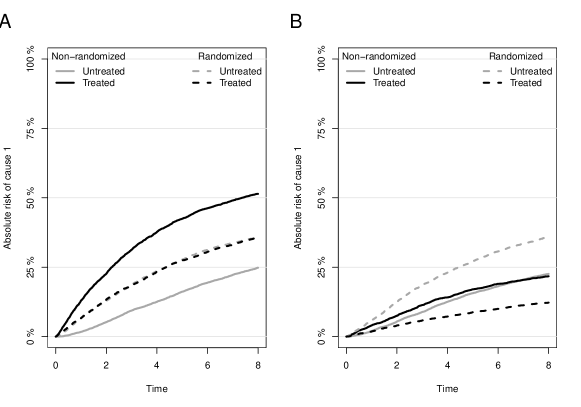
Figure 1: Illustration of the data generating mechanism used in our simulation studies. Shown are the Aalen-Johansen estimates for the absolute risks of cause 1 in both treatment arms in two independently drawn datasets (non-randomized and randomized) each of size n=10,000. Panel A: The treatment effect is zero. In the non-randomized world, the Aalen-Johansen estimate of the 8-year risk difference is large. Panel B: The treatment has a protective effect. In the non-randomized world, the Aalen-Johansen estimate of the 8-year risk difference is about zero.

For various parameter settings we report results of the estimators G-formula (equation 3), $\operatorname{IPTW},\operatorname{IPCW}$ (equation 6), and $\operatorname{AIPTW},\operatorname{AIPCW}$ (equation 9) across 1,000 simulated datasets. These estimators are implemented in R (R Core Team, 2018) in the package riskRegression (Gerds and Ozenne (2019), function ateRobust). When estimating the variance of the $\operatorname{AIPTW},\operatorname{AIPCW}$ estimators, we consider two estimators for the influence function. The first, denoted $\tilde{\mathrm{IF}}_{\operatorname{AIPTW},\operatorname{AIPCW}}$, only estimates the first term of equation (11) since the second term is 0 in correctly specified models. The second estimates both terms and is denoted $\mathrm{IF}_{\operatorname{AIPTW},\operatorname{AIPCW}}$. However we have not implemented all the terms necessary to compute $\phi_{\operatorname{AIPTW},\operatorname{AIPCW}}$: the current implementation is equivalent to neglecting the uncertainty relative to the censoring weights and the augmentation term $I(\tilde{T},\tau|A,W)$. The R-code of our simulation studies is available as supplementary material.

5.2 Simulation results

We report results for a data generating model without treatment effect (Panel A, Figure 1). The figure shows Aalen-Johansen estimates (Aalen and Johansen, 1978; Andersen et al., 1993) of the cumulative incidence functions. Similar results are obtained when considering a non-zero treatment effect but then the “true” value needs to be obtained empirically. Model misspecification is simulated by omitting covariates and quadratic effects. We created four scenarios. In the first one, all models are correctly specified. In the three other scenarios, precisely one of the censoring, outcome, or treatment models is misspecified. As shown in figure 2 (upper panel), the AIPTW,AIPCW estimator is consistent even when one of the models (outcome, treatment, or censoring) is misspecified. The G-formula estimator and the IPTW,IPCW estimator need one or two models to be correctly specified to be consistent - the outcome model for the G-formula estimator and both the treatment and censoring models for the IPTW,IPCW estimator. The G-formula estimator appears to be less variable compared to the other estimators. The IPTW,IPCW estimator is at least as variable but often more variable than the AIPTW,AIPCW estimator. The coverage of the G-formula estimator and AIPTW,AIPCW estimator is found satisfactory even in small samples when the outcome model is correctly specified (Figure 3).

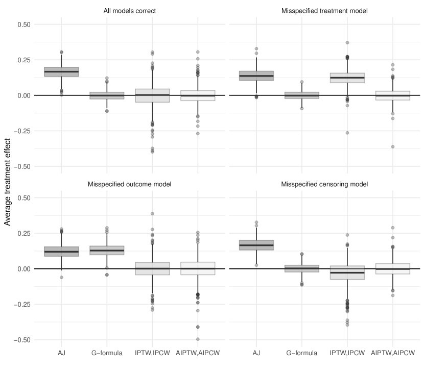
Figure 2: Simulation setting where there is no treatment effect (panel A of Figure 1). Boxplots show results of 1000 simulated data sets (each with sample size 500) and each of 4 methods for estimating the average 10-year risk difference between treated and untreated subjects. Upper left panel: all regression models (treatment, event of interest, competing risk, censoring) are correctly specified. Upper right panel: the treatment model is misspecified (missing covariates and missing quadratic effects). Lower left panel: the event of interest and the competing risk models are misspecified (missing covariates and missing quadratic effects). Lower right panel: the censoring model is misspecified (missing quadratic effects).

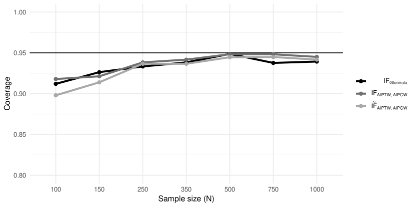
Figure 3: Effect of sample size on coverage in a simulation setting where there is no treatment effect (panel A of Figure 1). The black curve corresponds to the G-formula estimator, the dark grey curve to the $\operatorname{AIPTW},\operatorname{AIPCW}$ estimator using the full influence function to estimate the variance, and the light gray curve to the $\operatorname{AIPTW},\operatorname{AIPCW}$ estimator using only the first term of the influence function to estimate the variance.

6 Real data application

For the sole purpose of illustration, we consider a subset of the data presented in Stærk et al. (2018). This Danish registry study included n=21149 patients with a diagnosis of atrial fibrillation (AF) in the period 2012-2016 who initiated anticoagulation treatment with a standard dose of dabigatran (n=7078) or rivaroxaban (n=6868) or apixaban (n=7203). All three treatments belong to the group of non-vitamin K antagonist oral anticoagulants (NOAC’s). Here we consider only data from patients that initiated treatment with either dabigatran or rivaroxaban. The follow up started at the date of treatment initiation. The original study Stærk et al. (2018) presented results on several adverse endpoints including thromboembolism/stroke and major bleeding where death without the endpoint is the only competing risk. Here we consider the analysis of the endpoint major bleeding where death without major bleeding or shift or discontinuation of treatment are the competing risk. The treatment assignment is not randomized but there are official guidelines and presumably also doctor preferences which most likely also depend on the patient characteristics. Note that the results presented here for G-formula are not directly comparable to those presented in Stærk et al. (2018) because we here restrict all Cox regression models to the subset of the dabigatran and rivaroxaban patients. Otherwise we use the same covariate adjustment as described in detail in Stærk et al. (2018) for all Cox regression models and for the logistic regression model of the treatment mechanism. Figure 4 displays the estimates absolute risk of major bleeding obtained with G-formula and AIPTW,AIPCW. Within the limitation of the available confounder information the results can be interpreted as what one would have observed in a hypothetical world where all patients initiated dabigatran (or rivaroxaban), respectively.

The interpretation of these results is limited to the population of patients who initiated either dabigatran or rivaroxaban in the period 2012-2016. Based on the AIPTW,AIPCW estimate evaluated at 12 months, the interpretation could be as follows. If every patient had received dabigatran the 1-year risk [95% confidence interval] of a major bleeding would have been 1.58% [0.60;2.57] lower compared to when every patient had received rivaroxaban. Interestingly, the AIPTW,AIPCW estimates of the risk differences are larger in magnitude compared to the G-formula estimates. For example, the estimate of ATE (12-month) using G-formula is only 0.97% [0.40;1.54].

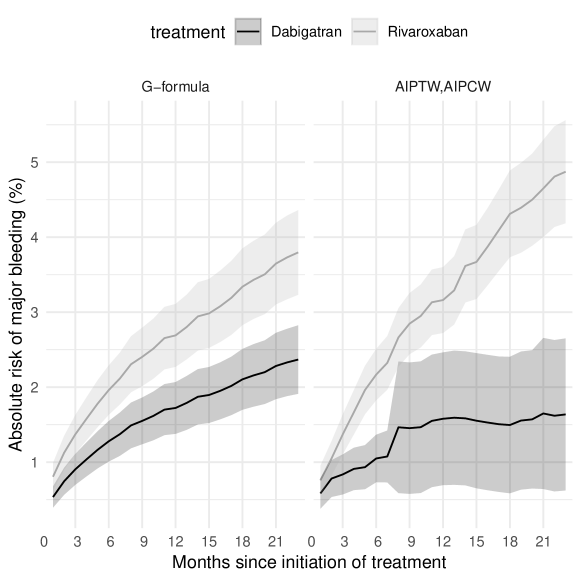
Figure 4: Illustration in data of Danish registry study. Lines are absolute risk estimates with time-pointwise 95% confidence limits using G-formula (left panel) and AIPTW,AIPCW (right panel).

7 Discussion

In presence of completely observed outcomes, estimation of the average treatment effect can be performed using estimators based on the G-formula, inverse probability of treatment weighting (IPTW), or a combination of both (AIPTW). While these are classical tools in causal inference (see for e.g., part 2 of Hernán and Robins (2019)), we review in this article their extension to right-censored data and to the presence of competing risks. Using results from semi-parametric theory, we derive the augmentation term relative to the working model for the censoring distribution. We investigate the robustness of this new estimator against misspecification of the working models. We also show the asymptotic normality of this estimator and derive an analytical formula for its influence function which can be used to estimate the variance of the estimator. The variance of our estimator may depend on the estimators of the nuisance parameters. In our software implementation (Gerds and Ozenne, 2019), we focus on the use of cause-specific Cox regression models for the outcome model, a logistic regression for the treatment model, and a Cox regression model for the censoring model. An alternative would be to use a Fine-Gray regression model for the outcome. However, then one would need an additional working regression model for the conditional event-free survival function $S(\cdot|A,W)$. To simplify the implementation, we currently do not estimate the variability related to the estimation of the censoring distribution $G(\cdot|A,W)$ and the augmentation term $I(\cdot,\tau|A,W)$. In to our simulation study this omission did not have a large effect and the coverage of our confidence intervals was sufficient.

The simulations confirm the superiority of the $\operatorname{AIPTW},\operatorname{AIPCW}$ estimator over the $\operatorname{IPTW},\operatorname{IPCW}$ estimator. They also show that the G-formula estimator is less variable than the $\operatorname{AIPTW},\operatorname{AIPCW}$ estimator when the outcome model is correctly specified. However, the G-formula estimator has a bias that the $\operatorname{AIPTW},\operatorname{AIPCW}$ estimator does not have when the outcome model is misspecified. It is worth noting that the definition of the G-formula estimator is unchanged in presence of censoring - only the outcome model has to properly handle censoring.

Competing risks essentially lead to a change of the definition of the outcome, where we use $\mathrm{1}{\{T\leq\tau,\Delta=1\}}$ instead of $\mathrm{1}{\{T\leq\tau\}}$. However one should not overlook that the presence of competing risks complexifies the assessment of the treatment effect, especially when the treatment has a positive effect on the cause of interest but a negative effect on the competing events. We refer to Young et al. (2018) for a detailed discussion of the implications of how the estimand is defined in presence of competing risks.

Recently, Lesko and Lau (2017) pointed out that bias will occur if we do not have the correct models for the probability of the outcome of interest $F_{1}(\tau|A,W)=\mathrm{P}[T\leq\tau,\Delta=1|A,W]$, in particular when the model for the hazard rate of the competing risk $\Lambda_{2}$ is misspecified. In practice this means that, if we estimate the outcome model via a cause-specific Cox regression models, both conditional hazard functions need to be correctly specified. While our approach relies on prior knowledge to define the working models, automated techniques and the use of cross-validation (Benkeser et al., 2018) may be preferable when prior knowledge is sparse. Indeed, the Cox regression model makes the assumption of proportional hazards which may not always be appropriate. This assumption can be relaxed, e.g., by using stratified baseline hazard functions, time varying coefficients (Martinussen and Scheike, 2007), or an alternative approach that does not rely on this assumption (e.g., using pseudo-observations (Andersen et al., 2017)).

We have focused on a binary treatment variable. In the case of a multi-valued treatment variable the several estimands can be defined depending on the type of the treatment variable (ordinal versus nominal), see Imbens (2000) for a nice discussion. One option is to compare each pair of treatments in the subpopulation of subjects treated with either of the treatments. This is what we have done in our real data analysis.

We have also focused on a single time point to evaluate the treatment effect. However, our methods can be extended to multiple time points, perhaps at the cost of a multiple testing issue.

Handling time-varying treatments and therefore possible time-varying confounding is more challenging and beyond the scope of this article; we refer the refer the interested reader to (Bekaert et al., 2010; Daniel et al., 2013; Moodie et al., 2014; Hernán and Robins, 2019).

8 Acknowledgment

B.M.H.O. was supported by Hjerteforeningen Forskningsstøtte (nr. 15-R99-A5954 015-S15), the Lundbeck foundation (R231-2016-3236) and Marie-Curie-NEUROMODEL (746850).

9 Conflict of interest

The authors have declared no conflict of interest.

Appendix

A Estimating equation for the $\operatorname{AIPTW}$,$\operatorname{AIPCW}$ estimator

For a generic individual with full data $O$, we denote by $m_{\operatorname{AIPTW}}$ the estimating function:

$$m_{\operatorname{AIPTW}}(\tau;O)= \,Y(\tau)\left(\frac{A}{\pi(W)}-\frac{1-A}{1-\pi(W)}\right)+F_{1}(\tau|A=1,W)\left(1-\frac{A}{\pi(W)}\right)$$

$$-F_{1}(\tau|A=0,W)\left(1-\frac{1-A}{1-\pi(W)}\right)-\Psi(\tau).$$

Semi-parametric theory (e.g., (Tsiatis, 2006) - chapter 9, formula 9.34) gives the following augmented estimating equation:

$$\sum_{i=1}^{n}\frac{\mathrm{1}{\{C_{i}>T_{i}\wedge\tau\}}m_{\operatorname{AIPTW}}(\tau;O_{i})}{G(\tilde{T}_{i}\wedge\tau|A_{i},W_{i})}-\int_{0}^{\tau\wedge\tilde{T}_{i}}\frac{f_{\operatorname{AIPTW}}(t,O_{i})}{G(t|A_{i},W_{i})}dM_{i}^{C}(t)=0$$

where $f_{\operatorname{AIPTW}}$ is an element of the space of real valued functions well-defined on the support of $(\tilde{T},\tilde{\Delta},A,W)$. To fully define the estimating equation it remains to define what is $f_{\operatorname{AIPTW}}$. It is reasonable to choose $f_{\operatorname{AIPTW}}$ such the estimator has the smallest asymptotic variance, i.e., its influence function has the smallest variance. Theorem 10.1 and 10.4 in (Tsiatis, 2006) gives that this is achieved by taking $f_{\operatorname{AIPTW}}(t;O)=-\mathrm{E}[m_{\operatorname{AIPTW}}(\tau;O)|T>t,A,W]$. It follows that:

$$f_{\operatorname{AIPTW}}(t;O)= -\left(\mathrm{E}\left[Y(\tau)|T>t,A,W\right]\left(\frac{A}{\pi(W)}-\frac{1-A}{1-\pi(W)}\right)-\Psi(\tau)\right.$$

$$\left.+F_{1}(\tau|A=1,W)\left(1-\frac{A}{\pi(W)}\right)-F_{1}(\tau|A=0,W)\left(1-\frac{1-A}{1-\pi(W)}\right)\right),$$

where

$$\mathrm{E}[Y(\tau)|T>t,A,W] =\mathrm{P}[T\leq\tau,\tilde{\Delta}=1|T>t,A,W]=\frac{\mathrm{P}[t<T\leq\tau,\tilde{\Delta}=1|A,W]}{\mathrm{P}[T>t|\tilde{\Delta},W]}$$

$$=\frac{\mathrm{P}[T\leq\tau,\tilde{\Delta}=1|A,W]-\mathrm{P}[T\leq t,\tilde{\Delta}=1|A,W]}{\mathrm{P}[T>t|A,W]}$$

$$=\frac{F_{1}(\tau|A,W)-F_{1}(t|A,W)}{S(t|A,W)}.$$

Since:

$$\int_{0}^{\tau\wedge\tilde{T}}\frac{1}{G(t|A,W)}dM^{C}(t) =\int_{0}^{\tau\wedge\tilde{T}}\exp(\Lambda^{C}(t|A,W))d(N_{C}(t)-\Lambda^{C}(t|A,W))$$

$$=1-\frac{\mathrm{1}{\{C>\tilde{T}\wedge\tau\}}}{G(\tilde{T}\wedge\tau|A,W)},$$ (14)

we obtain the augmented estimating equation for the $\operatorname{AIPTW}$ estimator:

$$0= \sum_{i=1}^{n}\frac{\mathrm{1}{\{C_{i}>T_{i}\wedge\tau\}}}{G(\tilde{T}_{i}\wedge\tau|A_{i},W_{i})}\left(Y_{i}(\tau)\left(\frac{A_{i}}{\pi(W_{i})}-\frac{1-A_{i}}{1-\pi(W_{i})}\right)+F_{1}(\tau|A=1,W_{i})\left(1-\frac{A_{i}}{\pi(W_{i})}\right)\right.$$

$$\qquad\qquad\qquad\qquad\qquad\left.-F_{1}(\tau|A=0,W_{i})\left(1-\frac{1-A_{i}}{1-\pi(W_{i})}\right)-\Psi(\tau)\right)$$

$$\qquad+\left(\frac{A_{i}}{\pi(W_{i})}-\frac{1-A_{i}}{1-\pi(W_{i})}\right)\int_{0}^{\tau\wedge\tilde{T}_{i}}\frac{F_{1}(\tau|A_{i},W_{i})-F_{1}(t|A_{i},W_{i})}{S(t|A_{i},W_{i})}\frac{1}{G(t|A_{i},W_{i})}dM_{i}^{C}(t)$$

$$\qquad+\left(F_{1}(\tau|A=1,W_{i})\left(1-\frac{A_{i}}{\pi(W_{i})}\right)-F_{1}(\tau|A=0,W_{i})\left(1-\frac{1-A_{i}}{1-\pi(W_{i})}\right)-\Psi(\tau)\right)$$

$$\qquad\qquad\qquad\left(1-\frac{\mathrm{1}{\{C_{i}>T_{i}\wedge\tau\}}}{G(\tilde{T}_{i}\wedge\tau|A_{i},W_{i})}\right),$$

i.e. denoting $I(\tilde{T}_{i},\tau|A_{i},W_{i})=\int_{0}^{\tau\wedge\tilde{T}_{i}}\frac{F_{1}(\tau|A_{i},W_{i})-F_{1}(t|A_{i},W_{i})}{S(t|A_{i},W_{i})}\frac{1}{G(t|A_{i},W_{i})}dM_{i}^{C}(t)$:

$$0= \sum_{i=1}^{n}\left(\frac{A_{i}}{\pi(W_{i})}-\frac{1-A_{i}}{1-\pi(W_{i})}\right)\left(\frac{Y_{i}(\tau)\mathrm{1}{\{C_{i}>T_{i}\wedge\tau\}}}{G(\tilde{T}_{i}\wedge\tau|A_{i},W_{i})}+I(\tilde{T}_{i},\tau|A_{i},W_{i})\right)$$

$$+F_{1}(\tau|A=1,W_{i})\left(1-\frac{A_{i}}{\pi(W_{i})}\right)-F_{1}(\tau|A=0,W_{i})\left(1-\frac{1-A_{i}}{1-\pi(W_{i})}\right)-\Psi(\tau).$$ (15)

Solving equation (15) gives the estimator defined in equation (9). Similar derivations for the $\operatorname{IPTW}$ estimator in presence of censoring lead to equation (8).

B Proof of theorem 1

Correctly specified censoring model: in this case $G^{*}$ and $M^{c,*}$ are equal to $G$ and $M^{c}$, respectively. We use the second notation and show that $\widehat{\Psi}_{\operatorname{AIPTW},\operatorname{AIPCW}}(\tau)$ and $\widehat{\Psi}_{\operatorname{AIPTW}}(\tau)$ have the same large sample limit. We denote by $\mathcal{F}_{t,i}$ the natural history up to time $t$ for individual i where $\mathcal{F}_{0,i}=(A_{i},W_{i})$. For $i\in\{1,\ldots,n\}$, $M_{i}^{C}(t)$ is a martingale satisfying $M_{i}^{C}(0)=0$. Since $F_{1}^{*}(\tau|A_{i},W_{i})$, $F_{1}^{*}(t|A_{i},W_{i})$, $S^{*}(t|A_{i},W_{i})$, and $G(t|A_{i},W_{i})$ are predictable with respect to $\mathcal{F}_{0,i}$, we obtain that:

$$\bar{I}(\tilde{T}_{i},\tau|A_{i},W_{i})=\int_{0}^{\tilde{T}_{i}\wedge\tau}\frac{F_{1}^{*}(\tau|A_{i},W_{i})-F_{1}^{*}(t|A_{i},W_{i})}{S^{*}(t|A_{i},W_{i})}\frac{1}{G(t|A_{i},W_{i})}dM_{i}^{C}(t)$$

is a martingale. Using that $\mathrm{E}[M_{i}^{C}(t)|\mathcal{F}_{0,i}]=0$, we get:

$$\mathrm{E}[\bar{I}(\tilde{T}_{i},\tau|A_{i},W_{i})]=\mathrm{E}[\mathrm{E}[\bar{I}(\tilde{T}_{i},\tau|A_{i},W_{i})|\mathcal{F}_{0,i}]]=0.$$

Therefore:

$$\mathrm{E}\left[\bar{I}(\tilde{T},\tau|A,W)\left(\frac{A}{\pi^{*}(W)}-\frac{1-A}{1-\pi^{*}(W)}\right)\right]=\mathrm{E}\left[\mathrm{E}[\bar{I}(\tilde{T},\tau|A,W)|\mathcal{F}_{0}]\left(\frac{A}{\pi^{*}(W)}-\frac{1-A}{1-\pi^{*}(W)}\right)\right]=0$$

where the outer expectation is taken over the joint distribution of $\tilde{T},A$ and $W$. Moreover:

$$\mathrm{E}\left[\frac{\mathrm{1}{\{\tilde{T}\leq\tau,\tilde{\Delta}\neq 0\}}}{G(\tilde{T}|A,W)}Y(\tau)\left(\frac{A}{\pi^{*}(W)}-\frac{1-A}{1-\pi^{*}(W)}\right)\right]$$

$$=\mathrm{E}\left[\mathrm{E}\left[\frac{\mathrm{1}{\{C>\tilde{T}\wedge\tau\}}}{G(\tilde{T}\wedge\tau|A,W)}\Bigg{|}A,W\right]\mathrm{E}\left[Y(\tau)\left(\frac{A}{\pi^{*}(W)}-\frac{1-A}{1-\pi^{*}(W)}\right)\Bigg{|}A,W\right]\right]$$

$$=\mathrm{E}\left[Y(\tau)\left(\frac{A}{\pi^{*}(W)}-\frac{1-A}{1-\pi^{*}(W)}\right)\right],$$

where we have used the conditional independent censoring assumption. So $\lim_{n\rightarrow\infty}\widehat{\Psi}_{\operatorname{AIPTW},\operatorname{AIPCW}}(\tau)=\lim_{n\rightarrow\infty}\widehat{\Psi}_{\operatorname{AIPTW}}(\tau)$ and 1. and 2. follow from the double robustness of $\widehat{\Psi}_{\operatorname{AIPTW}}(\tau)$.

Misspecified censoring model: We assume that the outcome model and survival model are correctly specified, i.e., $F_{1}^{*}=F_{1}$ and $S^{*}=S$. Using equation (14), we obtain:

$$\frac{Y_{i}(\tau)\mathrm{1}{\{\tilde{T}_{i}\leq\tau,\tilde{\Delta}\neq 0\}}}{G^{*}(\tilde{T}_{i}|A_{i},W_{i})}+\int_{0}^{\tilde{T}_{i}\wedge\tau}\frac{F_{1}^{*}(\tau|A_{i},W_{i})-F_{1}^{*}(t|A_{i},W_{i})}{S^{*}(t|A_{i},W_{i})G^{*}(t|A_{i},W_{i})}dM_{i}^{C,*}(t)$$

$$= Y_{i}(\tau)+\int_{0}^{\tilde{T}_{i}\wedge\tau}\frac{\frac{F_{1}(\tau|A_{i},W_{i})-F_{1}(t|A_{i},W_{i})}{S(t|A_{i},W_{i})}-Y_{i}(\tau)}{G^{*}(t|A_{i},W_{i})}dM_{i}^{C,*}(t)$$

$$= Y_{i}(\tau)+\int_{0}^{\tilde{T}_{i}\wedge\tau}\frac{\mathrm{E}[Y_{i}(\tau)|T_{i}>t,A_{i},W_{i}]-Y_{i}(\tau)}{G^{*}(t|A_{i},W_{i})}dM_{i}^{C,*}(t).$$

We now show that the second term has null expectation. Denoting $\epsilon_{i}(t)=\frac{\mathrm{E}[Y_{i}(\tau)|T_{i}>t,A_{i},W_{i})]-Y_{i}(\tau)}{G^{*}(t|A_{i},W_{i})}$ and using the conditional independent censoring assumption, we have that $\mathrm{E}[\epsilon_{i}(t)|T_{i}>t,A_{i},W_{i}]=0$. With $R_{i}(t)$ the at risk process, we can decompose the second term further in two terms:

$$\int_{0}^{\tilde{T}_{i}\wedge\tau}\epsilon_{i}(t)dM_{i}^{C,*}(t)=\int_{0}^{\tilde{T}_{i}\wedge\tau}\epsilon_{i}(t)dM_{i}^{C}(t)+\int_{0}^{\tilde{T}_{i}\wedge\tau}\epsilon_{i}(t)R_{i}(t)d\left(\Lambda^{C}(t|A_{i},W_{i})-\Lambda^{C,*}(t|A_{i},W_{i})\right)$$ (16)

The first term in (16) is a mean-zero martingale, and the second term in equation (16) also has mean zero since

$$\mathrm{E}\left[\int_{0}^{\tilde{T}_{i}\wedge\tau}R_{i}(t)\epsilon_{i}(t)\left(\lambda^{C}(t|A_{i},W_{i})-\lambda^{C,*}(t|A_{i},W_{i})\right)dt\Big{|}A_{i},W_{i}\right]$$

$$=\mathrm{E}\left[\int_{0}^{\tau}R_{i}(t)\epsilon_{i}(t)\left(\lambda^{C}(t|A_{i},W_{i})-\lambda^{C,*}(t|A_{i},W_{i})\right)dt\Big{|}A_{i},W_{i}\right]$$

$$=\int_{0}^{\tau}\mathrm{E}\left[R_{i}(t)\epsilon_{i}(t)|A_{i},W_{i}\right]\left(\lambda^{C}(t|A_{i},W_{i})-\lambda^{C,*}(t|A_{i},W_{i})\right)dt=0,$$

because $\mathrm{E}\left[R_{i}(t)\epsilon_{i}(t)|A_{i},W_{i}\right]=\mathrm{E}\left[R_{i}(t)\mathrm{E}[\epsilon_{i}(t)|T_{i}>t,A_{i},W_{i}]|A_{i},W_{i}\right]=0$. So the large sample limit of the $\operatorname{AIPTW},\operatorname{AIPCW}$ estimator is:

$$\lim_{n\rightarrow\infty}\widehat{\Psi}_{\operatorname{AIPTW},\operatorname{AIPCW}}(\tau)=\mathrm{E}\Bigg{[}F_{1}(\tau|A=1,W)-F_{1}(\tau|A=0,W)$$

$$+\left(\frac{A}{\pi^{*}(W)}-\frac{1-A}{1-\pi^{*}(W)}\right)\left(Y(\tau)-F_{1}(\tau|A,W)+\int_{0}^{\tilde{T}\wedge\tau}\epsilon(t)dM^{C,*}(t)\right)\Bigg{]}$$

$$=\mathrm{E}[F_{1}(\tau|A=1,W)-F_{1}(\tau|A=0,W)]$$

$$+\mathrm{E}\left[\left(\frac{A}{\pi^{*}(W)}-\frac{1-A}{1-\pi^{*}(W)}\right)\left(\mathrm{E}[Y(\tau)|A,W]-F_{1}(\tau|A,W)+\mathrm{E}\left[\int_{0}^{\tilde{T}\wedge\tau}\epsilon(t)dM^{C,*}(t)\Bigg{|}A,W\right]\right)\right]$$

$$=\mathrm{E}[F_{1}(\tau|A=1,W)-F_{1}(\tau|A=0,W)]$$

which also equals $\Psi(\tau)$.

C Influence function of the AIPTW,AIPCW estimator

We define the functional $\nu$ as a mapping of a set of probability measures to the real numbers such that for a probability measure $\mathrm{P}$:

$$\nu(\mathrm{P})=\nu_{1}(F_{1},\pi,S,G,\mathrm{P})-\nu_{0}(F_{1},\pi,S,G,\mathrm{P})$$

where, for $a\in\{0,1\}$ and denoting $\pi^{a}(W)=a\pi(W)+(1-a)(1-\pi(W))$, we have:

$$\nu_{a}(F_{1},\pi,S,G,\mathrm{P})=\mathrm{E}\Bigg{[}F_{1}(\tau|A=a,W)$$

$$+\frac{\mathrm{1}{\{A=a\}}}{\pi^{a}(W)}\left(Y(\tau)-F_{1}(\tau|A,W)+\int_{0}^{\tilde{T}\wedge\tau}\frac{\frac{F_{1}(\tau|A,W)-F_{1}(t|A,W)}{S(t|A,W)}-Y(\tau)}{G(t|A,W)}dM^{C}(t)\right)\Bigg{]}.$$

where the expectation is relative to the joint distribution of $A$ and $W$. By denoting $\mathrm{P}_{n}$ the empirical distribution function we have that $\nu(\mathrm{P}_{n})=\widehat{\Psi}_{\operatorname{AIPTW},\operatorname{AIPCW}}(\tau)$. So to obtain the influence function of the $\operatorname{AIPTW},\operatorname{AIPCW}$ estimator, we only need to derive the influence function associated with the estimator of $\nu_{a}$. Using Slutsky theorem, one can show that $\nu_{a}(\hat{F}_{1n},\hat{\pi}_{n},\hat{S}_{n},\hat{G}_{n},\mathrm{P}_{n})-\nu_{a}(F_{1}^{*},\hat{\pi}_{n},\hat{S}_{n},\hat{G}_{n},\mathrm{P}_{n})$ converges towards $\nu_{a}(\hat{F}_{1n},\pi^{*},S^{*},G^{*},\mathrm{P}_{n})-\nu_{a}^{*}$ where $\nu_{a}^{*}=\nu_{a}(F_{1}^{*},\pi^{*},S^{*},G^{*},\mathrm{P})$. Expanding with respect to each argument leads to:

$$\sqrt{n} \left(\nu_{a}(\hat{F}_{1n},\hat{\pi}_{n},\hat{S}_{n},\hat{G}_{n},\mathrm{P}_{n})-\nu_{a}^{*}\right)=\sqrt{n}\left(\nu_{a}(\hat{F}_{1n},\pi^{*},S^{*},G^{*},\mathrm{P})-\nu_{a}^{*}\right)$$

$$\quad+\sqrt{n}\left(\nu_{a}(F_{1}^{*},\hat{\pi}_{n},S^{*},G^{*},\mathrm{P})-\nu_{a}^{*}\right)+\sqrt{n}\left(\nu_{a}(F_{1}^{*},\pi^{*},\hat{S}_{n},G^{*},\mathrm{P})-\nu_{a}^{*}\right)$$

$$\quad+\sqrt{n}\left(\nu_{a}(F_{1}^{*},\pi^{*},S^{*},\hat{G}_{n},\mathrm{P})-\nu_{a}^{*}\right)+\sqrt{n}\left(\nu_{a}(F_{1}^{*},\pi^{*},S^{*},G^{*},\mathrm{P}_{n})-\nu_{a}^{*}\right)+o_{p}(1).$$

We can then calculate the influence function corresponding to each term:

$$\sqrt{n}\left(\nu_{a}(\hat{F}_{1n},\pi^{*},S^{*},G^{*},\mathrm{P})-\nu_{a}^{*}\right) =\frac{1}{\sqrt{n}}\sum_{i=1}^{n}\widetilde{}\mathrm{IF}_{\nu_{a},F_{1}}(\tau;O_{i})+o_{p}(1)$$

$$\sqrt{n}\left(\nu_{a}(F_{1}^{*},\hat{\pi}_{n},S^{*},G^{*},\mathrm{P})-\nu_{a}^{*}\right) =\frac{1}{\sqrt{n}}\sum_{i=1}^{n}\widetilde{}\mathrm{IF}_{\nu_{a},\pi}(\tau;O_{i})+o_{p}(1)$$

$$\sqrt{n}\left(\nu_{a}(F_{1}^{*},\pi^{*},\hat{S}_{n},G^{*},\mathrm{P})-\nu_{a}^{*}\right) =\frac{1}{\sqrt{n}}\sum_{i=1}^{n}\widetilde{}\mathrm{IF}_{\nu_{a},S}(\tau;O_{i})+o_{p}(1)$$

$$\sqrt{n}\left(\nu_{a}(F_{1}^{*},\pi^{*},S^{*},\hat{G}_{n},\mathrm{P})-\nu_{a}^{*}\right) =\frac{1}{\sqrt{n}}\sum_{i=1}^{n}\widetilde{}\mathrm{IF}_{\nu_{a},G}(\tau;O_{i})+o_{p}(1)$$

$$\sqrt{n}\left(\nu_{a}(F_{1}^{*},\pi^{*},S^{*},G^{*},\mathrm{P}_{n})-\nu_{a}^{*}\right) =\frac{1}{\sqrt{n}}\sum_{i=1}^{n}\widetilde{}\mathrm{IF}_{\nu_{a},\mathrm{P}}(\tau;O_{i})+o_{p}(1).$$

For instance, writing the difference between $\nu_{a}(F_{1}^{*},\pi^{*},S^{*},G^{*},\mathrm{P}_{n})$ and $\nu_{a}^{*}$ gives:

$$\widetilde{\mathrm{IF}}_{\nu_{a},\mathrm{P}}(\tau;O_{i})=F_{1}^{*}(\tau|A=a,W_{i})-\nu_{a}^{*}$$

$$+\frac{\mathrm{1}{\{A_{i}=a\}}}{\pi^{a,*}(W_{i})}\left(Y_{i}(\tau)-F_{1}^{*}(\tau|A_{i},W_{i})+\int_{0}^{\tilde{T}_{i}\wedge\tau}\frac{\frac{F_{1}^{*}(\tau|A_{i},W_{i})-F_{1}^{*}(t|A_{i},W_{i})}{S^{*}(t|A_{i},W_{i})}-Y_{i}(\tau)}{G^{*}(t|A_{i},W_{i})}dM_{i}^{C,*}(t)\right).$$

For $\widetilde{}\mathrm{IF}_{\nu_{a},F_{1}}$ we use that:

$$\sqrt{n}\left(\nu_{a}(\hat{F}_{1n},\pi^{*},S^{*},G^{*},\mathrm{P})-\nu^{*}_{a}\right)=$$

$$\frac{1}{\sqrt{n}}\sum_{i=1}^{n}\mathrm{E}\Bigg{[}\mathrm{IF}_{F_{1}^{*}}(\tau,a,W;O_{i})\left(1-\frac{\mathrm{1}{\{A=a\}}}{\pi^{a,*}(W)}\right)$$

$$\quad+\frac{\mathrm{1}{\{A=a\}}}{\pi^{a,*}(W)}\int_{0}^{\tilde{T}\wedge\tau}\frac{\mathrm{IF}_{F_{1}^{*}}(\tau,A,W;O_{i})-\mathrm{IF}_{F_{1}^{*}}(t,A,W;O_{i})}{S^{*}(t|A,W)G^{*}(t|A,W)}dM^{C,*}(t)\Bigg{|}O_{i}\Bigg{]}$$

where $\pi^{a,*}$ indicates the large sample limit of $\pi^{a}$ and $\mathrm{IF}_{F_{1}^{*}}(t,A,W,O_{i})$ is defined in equation (2). This leads to:

$$\widetilde{}\mathrm{IF}_{\nu_{a},F_{1}}(\tau;O_{i})= \mathrm{E}\Bigg{[}\mathrm{IF}_{F_{1}^{*}}(\tau,a,W;O_{i})\left(1-\frac{\mathrm{1}{\{A=a\}}}{\pi^{a,*}(W)}\right)$$

$$\qquad+\frac{\mathrm{1}{\{A=a\}}}{\pi^{a,*}(W)}\int_{0}^{\tilde{T}\wedge\tau}\frac{\mathrm{IF}_{F_{1}^{*}}(\tau,A,W;O_{i})-\mathrm{IF}_{F_{1}^{*}}(t,A,W;O_{i})}{S^{*}(t|A,W)G^{*}(t|A,W)}dM^{C,*}(t)\Bigg{|}O_{i}\Bigg{]}.$$

Similar derivations give:

$$\widetilde{\mathrm{IF}}_{\nu_{a},\pi}(\tau;O_{i})=-\mathrm{E}\Bigg{[}\mathrm{IF}_{\pi^{*}}(W;O_{i})\frac{\mathrm{1}{\{A=a\}}}{\left(\pi^{a,*}(W)\right)^{2}}\Bigg{(}\frac{Y(\tau)\mathrm{1}{\{\tilde{T}\leq\tau|\tilde{\Delta}\neq 0\}}}{G^{*}(\tilde{T}|A,W)}-F_{1}^{*}(\tau|A,W)$$

$$\qquad\qquad\qquad\qquad\qquad\qquad\qquad\qquad\qquad+\int_{0}^{\tilde{T}\wedge\tau}\frac{F_{1}^{*}(\tau|A,W)-F_{1}^{*}(t|A,W)}{S^{*}(t|A,W)G^{*}(t|A,W)}dM_{i}^{C,*}(t)\Bigg{)}\Bigg{|}O_{i}\Bigg{]}$$

$$\widetilde{\mathrm{IF}}_{\nu_{a},S}(\tau;O_{i})=-\mathrm{E}\Bigg{[}\frac{\mathrm{1}{\{A=a\}}}{\pi^{a,*}(W)}\int_{0}^{\tilde{T}\wedge\tau}\mathrm{IF}_{S^{*}}(t,A,W;O_{i})\frac{F_{1}^{*}(\tau|A,W)-F_{1}^{*}(t|A,W)}{S^{*}(t|A,W)^{2}G^{*}(t|A,W)}dM^{C,*}(t)\Bigg{|}O_{i}\Bigg{]}$$

$$\widetilde{\mathrm{IF}}_{\nu_{a},G}(\tau;O_{i})=-\mathrm{E}\Bigg{[}\frac{\mathrm{1}{\{A=a\}}}{\pi^{a,*}(W)}\left(\mathrm{IF}_{G^{*}}(\tilde{T},A,W;O_{i})\frac{Y(\tau)\mathrm{1}{\{\tilde{T}\leq\tau|\tilde{\Delta}\neq 0\}}}{G^{*}(\tilde{T}|A,W)^{2}}\right.$$

$$\qquad\qquad\qquad\qquad\qquad\qquad+\int_{0}^{\tilde{T}\wedge\tau}\mathrm{IF}_{G^{*}}(t,A,W;O_{i})\frac{F_{1}^{*}(\tau|A,W)-F_{1}^{*}(t|A,W)}{S^{*}(t|A,W)G^{*}(t|A,W)^{2}}dM^{C,*}(t)$$

$$\qquad\qquad\qquad\qquad\qquad\qquad\left.+\int_{0}^{\tilde{T}\wedge\tau}\frac{F_{1}^{*}(\tau|A,W)-F_{1}^{*}(t|A,W)}{S^{*}(t|A,W)G^{*}(t|A,W)}d\left(\mathrm{IF}_{\Lambda^{C,*}}(t,A,W;O_{i})\right)\right)\Bigg{|}O_{i}\Bigg{]}$$

where $\mathrm{IF}_{\Lambda^{C,*}}$ denotes the influence function of the cumulative hazard associated to the censoring mechanism. Furthermore, denoting

$$\mathrm{IF}_{\operatorname{AIPTW},\operatorname{AIPCW}}(\tau;O_{i})=\widetilde{}\mathrm{IF}_{\operatorname{AIPTW},\operatorname{AIPCW}}(\tau;O_{i})+\phi_{\operatorname{AIPTW},\operatorname{AIPCW}}(\tau;O_{i};\mathrm{IF_{F_{1}^{*}}},\mathrm{IF_{\pi^{*}}},\mathrm{IF_{S^{*}}},\mathrm{IF_{G^{*}}})$$

the influence function of the $\operatorname{AIPTW},\operatorname{AIPCW}$ estimator, we get that $\phi_{\operatorname{AIPTW},\operatorname{AIPCW}}(\tau;O_{i};\mathrm{IF_{F_{1}^{*}}},\mathrm{IF_{\pi^{*}}},\mathrm{IF_{S^{*}}},\mathrm{IF_{G^{*}}})$ equals

$$\widetilde{}\mathrm{IF}_{\nu_{1},F_{1}}(\tau;O_{i})+\widetilde{}\mathrm{IF}_{\nu_{1},\pi}(\tau;O_{i})+\widetilde{}\mathrm{IF}_{\nu_{1},S}(\tau;O_{i})+\widetilde{}\mathrm{IF}_{\nu_{1},G}(\tau;O_{i})$$

$$-\widetilde{}\mathrm{IF}_{\nu_{0},F_{1}}(\tau;O_{i})-\widetilde{}\mathrm{IF}_{\nu_{0},\pi}(\tau;O_{i})-\widetilde{}\mathrm{IF}_{\nu_{0},S}(\tau;O_{i})-\widetilde{}\mathrm{IF}_{\nu_{0},G}(\tau;O_{i})$$

and $\widetilde{}\mathrm{IF}_{\operatorname{AIPTW},\operatorname{AIPCW}}(\tau;O_{i})=\widetilde{}\mathrm{IF}_{\nu_{1},\mathrm{P}}(\tau;O_{i})-\widetilde{}\mathrm{IF}_{\nu_{0},\mathrm{P}}(\tau;O_{i})$.

Following the same reasoning as in the section B and using the conditional independence between the censoring mechanism and the treatment variable, we note that:

• $\widetilde{\mathrm{IF}}_{\nu_{a},F_{1}}=0$ when the treatment and censoring models are correctly specified.

• $\widetilde{\mathrm{IF}}_{\nu_{a},\pi}=0$ when the outcome and the censoring models are correctly specified.

• $\widetilde{\mathrm{IF}}_{\nu_{a},S}=0$ when the censoring is correctly specified.

• $\widetilde{\mathrm{IF}}_{\nu_{a},G}=0$ when the outcome, survival, and censoring models are correctly specified.

So when all models are correctly specified $\phi_{\operatorname{AIPTW},\operatorname{AIPCW}}(\tau;O_{i},\mathrm{IF}_{F_{1}^{*}},\mathrm{IF}_{\pi^{*}},\mathrm{IF}_{S^{*}},\mathrm{IF}_{G^{*}})=0$ and $\mathrm{IF}_{\operatorname{AIPTW},\operatorname{AIPCW}}(\tau;O_{i})=\widetilde{\mathrm{IF}}_{\operatorname{AIPTW},\operatorname{AIPCW}}(\tau;O_{i})$.

References

- Aalen and Johansen (1978) Aalen, O. and S. Johansen (1978). An empirical transition matrix for non-homogeneous Markov chains based on censored observations. Scandinavian Journal of Statistics 5, 141–150.
- Andersen et al. (1993) Andersen, P. K., Ø. Borgan, R. D. Gill, and N. Keiding (1993). Statistical Models Based on Counting Processes. Springer Series in Statistics. New York: Springer.
- Andersen et al. (2017) Andersen, P. K., E. Syriopoulou, and E. T. Parner (2017). Causal inference in survival analysis using pseudo-observations. Statistics in medicine 36(17), 2669–2681.
- Begun et al. (1983) Begun, J. M., W. Hall, W.-M. Huang, J. A. Wellner, et al. (1983). Information and asymptotic efficiency in parametric-nonparametric models. The Annals of Statistics 11(2), 432–452.
- Bekaert et al. (2010) Bekaert, M., S. Vansteelandt, and K. Mertens (2010). Adjusting for time-varying confounding in the subdistribution analysis of a competing risk. Lifetime data analysis 16(1), 45.
- Bender et al. (2005) Bender, R., T. Augustin, and M. Blettner (2005). Generating survival times to simulate Cox proportional hazards models. Statistics in medicine 24, 1713–1723.
- Benichou and Gail (1990) Benichou, J. and M. H. Gail (1990). Estimates of absolute cause-specific risk in cohort studies. Biometrics 46(3), 813–826.
- Benkeser et al. (2018) Benkeser, D., P. B. Gilbert, and M. Carone (2018). Estimating and testing vaccine sieve effects using machine learning. Journal of the American Statistical Association just-accepted, 1–29.
- Bickel et al. (1993) Bickel, P. J., C. A. Klaassen, Y. Ritov, and J. A. Wellner (1993). Efficient and Adaptive Estimation for Semiparametric Models. Johns Hopkins.
- Daniel et al. (2013) Daniel, R. M., S. Cousens, B. De Stavola, M. G. Kenward, and J. Sterne (2013). Methods for dealing with time-dependent confounding. Statistics in medicine 32(9), 1584–1618.
- Fine and Gray (1999) Fine, J. P. and R. J. Gray (1999). A proportional hazards model for the subdistribution of a competing risk. J. Amer. Statist. Assoc. 94, 496–509.
- Gerds and Schumacher (2001) Gerds, T. and M. Schumacher (2001). On functional misspecification of covariates in the Cox regression model. Biometrika 88(2), 572–580.
- Gerds and Ozenne (2019) Gerds, T. A. and B. Ozenne (2019). riskRegression: Risk Regression Models and Prediction Scores for Survival Analysis with Competing Risks. R package version 2019.03.03.
- Gill et al. (1995) Gill, R. D., M. J. Van der Laan, and J. M. Robins (1995). Coarsening at random: Characterizations, conjectures and counter-examples. In D. Y. Lin and T. R. Fleming (Eds.), Proceedings of the First Seattle Symposium in Biostatistics, pp. 255–294. Springer Lecture Notes in Statistics.
- Glynn and Quinn (2010) Glynn, A. N. and K. M. Quinn (2010). An introduction to the augmented inverse propensity weighted estimator. Political analysis 18(1), 36–56.
- Hernán and Robins (2006) Hernán, M. A. and J. M. Robins (2006). Instruments for causal inference: an epidemiologist’s dream? Epidemiology 17(4), 360–372.
- Hernán and Robins (2016) Hernán, M. A. and J. M. Robins (2016). Using big data to emulate a target trial when a randomized trial is not available. American journal of epidemiology 183(8), 758–764.
- Hernán and Robins (2019) Hernán, M. A. and J. M. Robins (2019). Causal inference. Boca Raton: Chapman & Hal/CRC, forthcoming.
- Hjort (1992) Hjort, N. L. (1992). On inference in parametric survival models. International Statistical Review 60, 355–387.
- Imbens (2000) Imbens, G. W. (2000). The role of the propensity score in estimating dose-response functions. Biometrika 87(3), 706–710.
- Kang et al. (2007) Kang, J. D., J. L. Schafer, et al. (2007). Demystifying double robustness: A comparison of alternative strategies for estimating a population mean from incomplete data. Statistical science 22(4), 523–539.
- Kennedy (2016) Kennedy, E. H. (2016). Semiparametric theory and empirical processes in causal inference. In Statistical Causal Inferences and Their Applications in Public Health Research, pp. 141–167. ICSA Book Series in Statistics. Springer, Cham.
- Lesko and Lau (2017) Lesko, C. R. and B. Lau (2017). Bias due to confounders for the exposure-competing risk relationship. Epidemiology (Cambridge, Mass.) 28(1), 20.
- Martinussen and Scheike (2007) Martinussen, T. and T. H. Scheike (2007). Dynamic regression models for survival data. Springer Science & Business Media.
- Moodie et al. (2014) Moodie, E. E., D. A. Stephens, and M. B. Klein (2014). A marginal structural model for multiple-outcome survival data: assessing the impact of injection drug use on several causes of death in the canadian co-infection cohort. Statistics in medicine 33(8), 1409–1425.
- Ozenne et al. (2017) Ozenne, B., A. L. Sørensen, T. Scheike, C. Torp-Pedersen, and T. A. Gerds (2017). riskregression: Predicting the risk of an event using Cox regression models. R Journal 9(2), 440–460.
- Pearl (2000) Pearl, J. (2000). Causality, models, reasoning and inference.
- R Core Team (2018) R Core Team (2018). R: A Language and Environment for Statistical Computing. Vienna, Austria: R Foundation for Statistical Computing.
- Robins (1986) Robins, J. (1986). A new approach to causal inference in mortality studies with a sustained exposure period – application to control of the healthy worker survivor effect. Mathematical modelling 7(9-12), 1393–1512.
- Scheike et al. (2008) Scheike, T., M. Zhang, and T. Gerds (2008). Predicting cumulative incidence probability by direct binomial regression. Biometrika 95(1), 205–220.
- Stærk et al. (2018) Stærk, L., T. Gerds, G. Y. Lip, B. Ozenne, A. Bonde, M. Lamberts, E. Fosbøl, C. Torp-Pedersen, G. Gislason, and J. Olesen (2018). Standard and reduced doses of dabigatran, rivaroxaban and apixaban for stroke prevention in atrial fibrillation: a nationwide cohort study. Journal of internal medicine 283(1), 45–55.
- Tsiatis (2006) Tsiatis, A. (2006). Semiparametric theory and missing data. Springer Verlag.
- van der Laan and Robins (2003) van der Laan, M. J. and J. M. Robins (2003). Unified Methods for Censored Longitudinal Data and Causality. Springer.
- van der Vaart (1998) van der Vaart, A. W. (1998). Asymptotic Statistics. Cambridge University Press.
- Wang et al. (2016) Wang, X., L. A. Beste, M. M. Maier, and X.-H. Zhou (2016). Double robust estimator of average causal treatment effect for censored medical cost data. Statistics in medicine 35(18), 3101–3116.
- White (1982) White, H. (1982). Maximum likelihood estimation of misspecified models. Econometrica 50, 1–25.
- Young et al. (2018) Young, J. G., E. J. T. Tchetgen, and M. A. Hernán (2018). The choice to define competing risk events as censoring events and implications for causal inference.
- Zhao et al. (2014) Zhao, Y.-Q., D. Zeng, E. B. Laber, R. Song, M. Yuan, and M. R. Kosorok (2014). Doubly robust learning for estimating individualized treatment with censored data. Biometrika 102(1), 151–168.