Single-jet inclusive rates with exact color at $\mathcal{O}(\alpha_{s}^{4})$

Abstract

Next-to-next-to-leading order QCD predictions for single-, double- and even triple-differential distributions of jet events in proton-proton collisions have recently been obtained using the NNLOjet framework based on antenna subtraction. These results are an important input for Parton Distribution Function fits to hadron-collider data. While these calculations include all of the partonic channels occurring at this order of the perturbative expansion, they are based on the leading-color approximation in the case of channels involving quarks and are only exact in color in the pure-gluon channel. In the present publication, we verify that the sub-leading color effects in the single-jet inclusive double-differential cross sections are indeed negligible as far as phenomenological applications are concerned. This is the first independent and complete calculation for this observable. We also take the opportunity to discuss the necessary modifications of the sector-improved residue subtraction scheme that made this work possible.

1 Introduction

Pure jet observables are not only interesting within the portfolio of Standard Model (SM) measurements but also as tools for New Physics searches. When paired with high-precision predictions within Quantum Chromodynamics (QCD), they are an important input for Parton Distribution Function (PDF) fits. Consistency of the latter application requires theoretical predictions at the same order of perturbation theory as the specified accuracy of the given PDF set. In consequence, it is nowadays indispensable to determine differential distributions of jet events at the next-to-next-to-leading order (NNLO) in QCD. Although not the subject of the present publication, non-perturbative effects from underlying event and hadronisation Khachatryan:2016wdh as well as electroweak corrections Dittmaier:2012kx should also be included for a realistic comparison with measurement data.

A calculation of jet rates at NNLO in QCD remains a very challenging project. Until now, results could only have been obtained with the help of the antenna subtraction scheme GehrmannDeRidder:2005cm ; GehrmannDeRidder:2005hi ; GehrmannDeRidder:2005aw ; Daleo:2006xa ; Daleo:2009yj ; Boughezal:2010mc ; Gehrmann:2011wi ; GehrmannDeRidder:2012ja ; Currie:2013vh ; Bernreuther:2011jt ; Bernreuther:2013uma ; Abelof:2011jv ; Abelof:2012he ; Abelof:2014fza as implemented in the NNLOjet framework Currie:2018oxh . While early studies concentrated on the pure-gluon case Currie:2013dwa ; Ridder:2013mf , several publications Currie:2017eqf ; Currie:2016bfm ; Gehrmann-DeRidder:2019ibf ; Currie:2018xkj appeared recently that present results including the complete set of partonic channels. It turns out that quark–gluon and quark–quark scattering dominates jet rates at high transverse momenta and/or rapidities. These contributions are, therefore, necessary for a complete description. On the other hand, the current NNLOjet implementation is based on the leading-color approximation for all channels but the pure-gluon channel. It has been argued in the past that inclusion of the sub-leading color effects at $\mathcal{O}(\alpha_{S}^{4})$ while keeping exact color dependence for the lower order contributions will have a negligible impact on the predictions. Nevertheless, it is necessary to verify this statement by explicit calculation. This is the main purpose of the present publication.

The published results on jet rates correspond to several different setups. In particular, Currie:2017eqf ; Currie:2016bfm correspond to 7 TeV ATLAS data, while Gehrmann-DeRidder:2019ibf to 8 TeV and Currie:2018xkj to 13 TeV CMS data. Single-jet inclusive cross sections (every identified jet in an event is accounted for in the histogram) that are double-differential in the jet transverse momentum, $p_{T}$, and rapidity, $|y|$, have been published for 7 and 13 TeV Large Hadron Collider (LHC) center-of-mass energies and various jet radii, $R$, defined with the anti-$k_{T}$ jet algorithm Cacciari:2008gp . Furthermore, for the same center-of-mass energies, there are available results for di-jet cross sections that are double differential in the di-jet invariant mass, $m_{jj}$, and the jet rapidity difference, $|y^{*}|\equiv|y_{1}-y_{2}|/2$. Finally, there is a published result for di-jet cross sections corresponding to 8 TeV CMS data that is triple-differential in the average transverse momentum, $p_{T,\mathrm{avg}}\equiv(p_{T,1}+p_{T,2})/2$, rapidity difference, $|y^{*}|$, and the boost, $y_{b}\equiv|y_{1}+y_{2}|/2$. For convenience of the reader, we summarise the available results in Appendix A.

Di-jet cross sections have consistently been evaluated with central renormalisation and factorisation scales $\mu_{R}=\mu_{F}=\mu=m_{jj}$. However, it turned out that the scale choice for single-jet inclusive cross sections is a non-trivial issue, since seemingly well-justified choices lead to large differences in the predictions as illustrated by the results for 7 TeV center-of-mass energy using the customary scales $\mu=p_{T}$ (each jet input into the histogram with the cross section evaluated with the scale equal to that particular jet transverse momentum) and $\mu=p_{T,1}$ (cross section scale set to the hardest-jet transverse momentum). The question of scale setting has been very thoroughly studied in Currie:2018xkj . The final recommendation of that publication is to use either the jet-based scale $\mu=2p_{T}$ or the event-based scale $\mu=\hat{H}_{T}$ (the scalar sum of the transverse momenta of the partons in the event).

The high computational cost of the calculation of jet rates with our software (see Section 3) enabled us to only perform one complete Monte Carlo simulation for the present publication. Since the setups of the different theoretical predictions described above differ in energy, jet transverse momentum cuts and jet radii, we had to choose a single specific setup to study the sub-leading color effects. Our goal was to compare results for a classic observable used in PDF fits that has been previously evaluated with one of the recommended scales. In view of these considerations, we have chosen to evaluate the single-jet inclusive cross section for 13 TeV center-of-mass energy available from Currie:2018xkj (jet radius $R=0.7$) using the jet-based scale $\mu=2p_{T}$. We should also point out that there are no available numerical values for cross sections or cross sections ratios in any of the publications Currie:2017eqf ; Currie:2016bfm ; Gehrmann-DeRidder:2019ibf ; Currie:2018xkj - only histograms have been provided. Appendix D contains our results for the K-factors, i.e. ratios of cross sections evaluated at NNLO and NLO in QCD with the same PDF set. This is a first step towards an easy inclusion of jet data in NNLO PDF fits. In the future, it would certainly be desirable to provide fastNLO Kluge:2006xs ; Wobisch:2011ij ; Britzger:2012bs or APPLGRID Carli:2010rw tables for all setups. We intend to undertake this task once more computational resources become available.

Besides the study of sub-leading color effects in jet rates, there is another aspect to the present publication. The calculation of a cross section at NNLO in QCD requires a method to handle infrared (IR) singularities occurring in contributions of different final state multiplicities. Apart from the already mentioned antenna subtraction scheme, there are several other methods currently being developed for this purpose: the CoLoRfulNNLO scheme Somogyi:2005xz ; Somogyi:2006da ; Somogyi:2006db ; Aglietti:2008fe ; DelDuca:2013kw , $q_{T}$-slicing Catani:2007vq ; Bonciani:2015sha , $N$-jettiness slicing Gaunt:2015pea ; Boughezal:2015dva ; Boughezal:2016zws ; Moult:2016fqy ; Moult:2017jsg ; Ebert:2018lzn ; Boughezal:2018mvf ; Boughezal:2019ggi , sector-improved residue subtraction Czakon:2010td ; Czakon:2011ve ; Czakon:2014oma and its spin-off called nested soft-collinear subtraction scheme Caola:2017dug ; Caola:2019nzf ; Caola:2019pfz , the projection-to-Born method Cacciari:2015jma ; Currie:2018fgr , local analytic sector subtraction Magnea:2018hab and geometric IR subtraction Herzog:2018ily . The results that we report in Section 3 have been obtained with our implementation of the sector-improved residue subtraction in the C++ library Stripper (SecToR Improved Phase sPacE for real Radiation). However, we have introduced several improvements w.r.t. to Ref. Czakon:2014oma . These improvements imply for instance a minimal number of subtraction terms per phase space point. They also require a modified reduction of the construction in Conventional Dimensional Regularisation (CDR) to four dimensions (’t Hooft-Veltman scheme). In the present publication, we discuss these issues in detail.

The paper is organised as follows. In the next section, we discuss modifications of the sector-improved residue subtraction. These consist of an improved phase space parameterisation and a new approach to the dimensional reduction of the formulation of the scheme. The section is closed with details on the implementation and tests. Subsequently, we present our results for the single-jet inclusive cross sections at 13 TeV. The main text is closed with an outlook. Appendices provide an overview of published results on jet cross sections, define the notation for cross section contributions, provide a list of expressions necessary for the implementation of the subtraction scheme in four dimensions, and, finally, provide numerical values of the NNLO K-factors.

2 Minimal sector-improved residue subtraction

We define a subtraction scheme to be minimal, if it has the minimal number of subtraction terms (defined by final state kinematics) for a given phase space point. Consider a phase space configuration with $n+2$ final state particles contributing to a cross section at next-to-next-to-leading order of perturbation theory. A configuration corresponding to a single soft (one gluon with vanishing energy) or collinear (two partons collinear) limit will have $n+1$ resolved final state particles (single-unresolved configuration), while a configuration corresponding to a double-soft (two gluons or a quark-anti-quark pair with vanishing energy) or triple-collinear (three partons collinear) limit will have $n$ resolved final state particles (double-unresolved configuration). Let us divide the phase space into sectors according to collinear limits (see Section 3 of Ref. Czakon:2014oma for more details). A sector that only allows for one singular configuration (divergent cross section contribution) in a specific single collinear limit is called single-collinear. A sector that allows for one singular configuration in a specific limit of two pairs of collinear partons is called double-collinear. Finally, a sector that allows for one singular configuration in a specific limit of three collinear partons is called triple-collinear. It is easy to convince one-self that the minimal number of subtraction terms in a single-collinear sector is one. Similarly, the minimal number of subtraction terms in a double-collinear sector is three (two for single-unresolved configurations and one for the double-unresolved configuration). Finally, the minimal number of subtraction terms in a triple-collinear sector is four (three for single-unresolved configurations and one for the double-unresolved configuration). The phase space construction of the sector-improved residue subtraction scheme as defined in Ref. Czakon:2014oma generates more subtraction terms. Here, we present an alternative parameterization of the phase space that, due to the additional sector decomposition in the triple-collinear sector, never requires more than three subtraction terms for a given phase space point. It turns out, however, that the four-dimensional formulation of the scheme requires modifications with this phase space. On the other hand, the methods presented here allow for numerical checks of pole cancellation in CDR for a fixed Born phase space point Behring:2018cvx ; PhDthesisPoncelet . In contrast, an implementation of Ref. Czakon:2014oma yields finite results at the level of distributions only.

We note, finally, that a single subtraction configuration in single-collinear parameterisations has also been obtained in the FKS subtraction scheme Frixione:1995ms implementations of Refs. Frixione:2002ik ; Frixione:2007vw . The approach presented here is conceptually different, and allows to cover next-to-leading and next-to-next-leading order cases on the same footing. It might be extensible to even higher orders.

2.1 Modified phase space parameterisations

2.1.1 Phase space mapping

Let us introduce the following notation for the phase space measure corresponding to a single particle with mass $m\geq 0$ and momentum $k$ in $d$ dimensions

$$\mathrm{d}\mu_{m}(k)\equiv\frac{\mathrm{d}^{d}k}{(2\pi)^{d}}\,2\pi\delta\big{(}k^{2}-m^{2}\big{)}\theta\big{(}k^{0}\big{)}\equiv\frac{\mathrm{d}^{d}k}{(2\pi)^{d}}\,2\pi\delta_{+}\big{(}k^{2}-m^{2}\big{)}\;.$$ (1)

The complete phase space for a process involving $n_{q}\neq 0$ (not explicitly parameterised) resolved momenta $q_{i}$, $n_{u}=1,2$ unresolved momenta $u_{i}=u_{i}^{0}\hat{u}_{i}$, and $0<n_{r}\leq n_{u}$ reference momenta $r_{i}$, $n_{fr}$ of which are in the final state, can be decomposed as follows

$$\begin{split}\mathrm{d}\bm{\Phi}_{n}&=\prod_{i=1}^{n_{q}}\mathrm{d}\mu_{m_{i}}(q_{i})\prod_{j=1}^{n_{fr}}\mathrm{d}\mu_{0}(r_{j})\prod_{k=1}^{n_{u}}\mathrm{d}\mu_{0}(u_{k})\,(2\pi)^{d}\delta^{(d)}\Big{(}\sum_{i=1}^{n_{q}}q_{i}+\sum_{j=1}^{n_{fr}}r_{j}+\sum_{k=1}^{n_{u}}u_{k}-P\Big{)}\\[5.69046pt] &=\frac{\mathrm{d}Q^{2}}{2\pi}\,\mathrm{d}\mu_{Q}(q)\prod_{j=1}^{n_{fr}}\mathrm{d}\mu_{0}(r_{j})\prod_{k=1}^{n_{u}}\mathrm{d}\mu_{0}(u_{k})\,(2\pi)^{d}\delta^{(d)}\Big{(}q+\sum_{j=1}^{n_{fr}}r_{j}+\sum_{k=1}^{n_{u}}u_{k}-P\Big{)}\\[5.69046pt] &\qquad\times\prod_{i=1}^{n_{q}}\mathrm{d}\mu_{m_{i}}(q_{i})\,(2\pi)^{d}\delta^{(d)}\Big{(}\sum_{i=1}^{n_{q}}q_{i}-q\Big{)}\\[5.69046pt] &=\mathrm{d}Q^{2}\Bigg{[}\prod_{j=1}^{n_{fr}}\mathrm{d}\mu_{0}(r_{j})\prod_{k=1}^{n_{u}}\mathrm{d}\mu_{0}(u_{k})\,\delta_{+}\Big{(}\Big{(}P-\sum_{j=1}^{n_{fr}}r_{j}-\sum_{k=1}^{n_{u}}u_{k}\Big{)}^{2}-Q^{2}\Big{)}\Bigg{]}\\[5.69046pt] &\qquad\times\prod_{i=1}^{n_{q}}\mathrm{d}\mu_{m_{i}}(q_{i})\,(2\pi)^{d}\delta^{(d)}\Big{(}\sum_{i=1}^{n_{q}}q_{i}-q\Big{)}\;,\end{split}$$ (2)

where $n=n_{q}+n_{fr}+n_{u}$ and $P$ is the total initial state momentum. In the second line, we have inserted an intermediate momentum $q$ with invariant mass $Q\geq\sum_{i=1}^{n_{q}}m_{i}$. In the third line, however, we have performed the integration over $q$, leaving an integration measure in the square brackets, which only depends on the fixed invariant mass of $q$.

The reference and unresolved momenta are the momenta that are allowed to correspond to a singular configuration in a given sector. Reference momenta and unresolved momenta have different behaviour w.r.t. the soft limit: a soft reference momentum does not generate a singularity. In case of a single- and triple-collinear sector one reference momentum $r$ is needed, while in the double-collinear sectors two reference momenta $r_{1}$ and $r_{2}$ are required.

We now introduce a mapping from the full phase space to the Born phase space

$$\{P,r_{j},u_{k}\}\,\longrightarrow\,\{\tilde{P},\tilde{r}_{j}\}\;,$$ (3)

which is invertible for fixed unresolved momenta

$$\{\tilde{P},\tilde{r}_{j},u_{k}\}\,\longrightarrow\,\{P,r_{j},u_{k}\}\;,$$ (4)

and which conserves the invariant mass of the intermediate state $q$

$$\tilde{q}^{2}=q^{2}\;,\quad\tilde{q}=\tilde{P}-\sum_{j=1}^{n_{fr}}\tilde{r}_{j}\;.$$ (5)

The mapping only involves a rescaling of the reference momenta. Specifically, for a final state reference momentum we require

$$r=x\,\tilde{r}\;,$$ (6)

where $x$ is given by a function $f_{x}$ of the full kinematics, in particular of $r$. The phase space measure is modified

$$\begin{split}\mathrm{d}\mu_{0}(r)&=\mathrm{d}\mu_{0}(r)\,\mathrm{d}x\,\delta\big{(}x-f_{x}(r)\big{)}\,\mathrm{d}^{d}\tilde{r}\,\delta^{(d)}(\tilde{r}-r/x)\\[5.69046pt] &=\mathrm{d}\mu_{0}(\tilde{r})\,\mathrm{d}x\,\theta(x)\,x^{d-2}\,\delta\big{(}x-f_{x}(x\,\tilde{r})\big{)}\\[5.69046pt] &=\mathrm{d}\mu_{0}(\tilde{r})\,\theta(x)\,x^{d-3}\Bigg{[}-\frac{\partial}{\partial x}\frac{f_{x}(x\,\tilde{r})}{x}\Bigg{]}^{-1}\Bigg{|}_{x=f_{x}(x\,\tilde{r})}\;.\end{split}$$ (7)

For an initial state reference, we require similarly

$$r=\tilde{r}/z\;,$$ (8)

where $z$ is given by a function $f_{z}$ of the full kinematics, in particular of $r$. We consider the phase space measure together with the integration over the parton momentum fraction $x$ with the parton distribution function $\phi$

$$\begin{split}\mathrm{d}x\,\phi(x)&=\mathrm{d}x\,\phi(x)\,\mathrm{d}\tilde{x}\,\delta\big{(}\tilde{x}-f_{z}(x\,p_{h})\,x\big{)}\\[5.69046pt] &=\mathrm{d}\tilde{x}\,\phi(\tilde{x}/z)\,\theta(z-\tilde{x})\Bigg{[}-z^{2}\frac{\partial}{\partial z}\frac{f(\tilde{r}/z)}{z}\Bigg{]}^{-1}\Bigg{|}_{z=f(\tilde{r}/z)}\;,\end{split}$$ (9)

where $p_{h}$ is the initial state hadron momentum.

The Born configuration is only properly defined, i.e. physical, if the rescaling parameters are always non-negative and $\tilde{q}^{0}\geq 0$. The phase space measure may be rewritten as

$$\begin{split}\mathrm{d}\bm{\Phi}_{n}&=\mathrm{d}Q^{2}\Bigg{[}\prod_{j=1}^{n_{fr}}\mathrm{d}\mu_{0}(\tilde{r}_{j})\,\delta_{+}\Big{(}\Big{(}\tilde{P}-\sum_{j=1}^{n_{fr}}\tilde{r}_{j}\Big{)}^{2}-Q^{2}\Big{)}\prod_{k=1}^{n_{u}}\mathrm{d}\mu_{0}(u_{k})\,\theta\big{(}\{u_{l}\}\in\mathcal{U}\big{)}\,\mathcal{J}\Bigg{]}\\[5.69046pt] &\qquad\times\prod_{i=1}^{n_{q}}\mathrm{d}\mu_{m_{i}}(q_{i})\,(2\pi)^{d}\delta^{(d)}\Big{(}\sum_{i=1}^{n_{q}}q_{i}-\tilde{q}\Big{)}\;,\end{split}$$ (10)

where $\theta\big{(}\{u_{l}\}\in\mathcal{U}\big{)}$ represents constraints on the unresolved momenta, and $\mathcal{J}$ is the Jacobian of the transformation. Furthermore, we have used Eq. (5) and the implied existence of a Lorentz transformation $\Lambda$, $q=\Lambda\,\tilde{q}$, together with the Lorentz invariance of $\mathrm{d}\mu_{m_{i}}(q_{i})$. The Born phase space measure is clearly singled out, which leads to the following algorithm for the construction of the full phase space

1. generate a Born configuration;

2. generate unresolved momenta subject to constraints;

3. determine the rescaling parameters and, by the same, the full reference momenta;

4. determine the Lorentz transformation yielding $q$ from $\tilde{q}$, and apply it to the final state momenta of the Born configuration;

5. multiply the weight by the Jacobian.

One advantage of this procedure is that it allows for the use of a multi-channel phase space generator for the Born configuration, which is particularly useful in case of intermediate resonances. Furthermore, electroweak decays should not affect efficiency, since intermediate invariant masses are not modified in the absence of QCD radiation from the decay products.

The rescaling parameters are fixed by Eq. (5) and an additional constraint in the case of two references (see section 2.1.4). The relations always involve a sum (final state reference) or a difference (initial state reference) of a reference momentum and an unresolved momentum. Thus, if $u=\alpha\,r$ (collinear or soft limit), for some unresolved, $u$, and reference, $r$, momenta, then the constraints fix $r\pm u$ (the observable or initial state momentum) independently of $u$. This is the reason for the minimal number of subtraction kinematics in all cases but the single-unresolved configurations of the triple-collinear parameterisation (see Section 2.1.3).

In the case of initial state references, the energy and rapidity of the initial state is modified. In order to have a minimal number of configurations, it is necessary to choose a frame with constant boost w.r.t. the laboratory, e.g. the laboratory frame or the center-of-mass frame of the underlying Born configuration. On the other hand, the center-of-mass frame of the $(n+n_{u})$-configuration cannot be used as it does not satisfy this constraint.

The same $(n+n_{u})$-configuration corresponds to different Born configurations for different parameterisations (single-collinear, triple-collinear and double-collinear). Thus, if the angles and energies of the unresolved momenta are required to have the same meaning across parameterisations, it is not possible to use the center-of-mass frame of the Born configuration either. This is important, since using the same angle and energy definition for all configurations yields simpler ’t Hooft-Veltman corrections. For this reason we use the laboratory system in the construction of the phase space.

2.1.2 One reference momentum

We explicitly treat the triple-collinear parameterisation. The single-collinear case is recovered by setting $u_{2}=0$. The following constraints determine $x$ or $z$

final state reference: initial state reference:

$$\big{(}P-r-u_{1}-u_{2}\big{)}^{2}=\big{(}P-\tilde{r}\big{)}^{2}\;, \big{(}r+p-u_{1}-u_{2}\big{)}^{2}=\big{(}\tilde{r}+p\big{)}^{2}\;,$$

$$x=\frac{P\cdot r}{(P-r)\cdot(r+u_{1}+u_{2})-u_{1}\cdot u_{2}}\;, z=\frac{(r+p)\cdot(r-u_{1}-u_{2})+u_{1}\cdot u_{2}}{p\cdot r}\;,$$

$$x=\frac{P\cdot(\tilde{r}-u_{1}-u_{2})+u_{1}\cdot u_{2}}{(P-u_{1}-u_{2})\cdot\tilde{r}}\;, z=\frac{(p-u_{1}-u_{2})\cdot\tilde{r}}{p\cdot(\tilde{r}+u_{1}+u_{2})-u_{1}\cdot u_{2}}\;,$$

$$\big{(}u_{1}^{0}\big{)}_{\mathrm{\max}}=\frac{P\cdot\tilde{r}}{P\cdot\hat{u}_{1}}\;, \big{(}u_{1}^{0}\big{)}_{\mathrm{\max}}=(1-\tilde{x})\frac{p\cdot\tilde{r}/\tilde{x}}{(\tilde{r}/\tilde{x}+p)\cdot\hat{u}_{1}}\;,$$

$$\big{(}u_{2}^{0}\big{)}_{\mathrm{\max}}=\frac{P\cdot(\tilde{r}-u_{1})}{(P-u_{1})\cdot\hat{u}_{2}}\;, \big{(}u_{2}^{0}\big{)}_{\mathrm{\max}}=\frac{(\tilde{r}/\tilde{x}+p)\cdot\big{(}(1-\tilde{x})\,\tilde{r}/\tilde{x}-u_{1}\big{)}}{(\tilde{r}/\tilde{x}+p-u_{1})\cdot\hat{u}_{2}}\;,$$

$$\mathcal{J}=\frac{x^{d-3}\,P\cdot\tilde{r}}{(P-u_{1}-u_{2})\cdot\tilde{r}}\;, \mathcal{J}=\frac{p\cdot\tilde{r}}{(p-u_{1}-u_{2})\cdot\tilde{r}}\;.$$

They have the following properties

1. the Born configuration is well defined for any full configuration, i.e. $x,z,\tilde{q}^{0}\geq 0$, and $x,z\leq 1$,

2. $x$, $z$ are monotonically decreasing functions of $u_{i}^{0}$, if $u_{j}$ with $i\neq j$ is fixed.

In consequence, an iterative energy parameterisation with $u_{1}^{0}$ determined in the range $\big{[}0,\,\big{(}u_{1}^{0}\big{)}_{\mathrm{max}}\big{]}$, followed by $u_{2}^{0}$ in the range $\big{[}0,\,\big{(}u_{2}^{0}\big{)}_{\mathrm{max}}(u_{1})\big{]}$ covers the full phase space. The maxima of the energies, $\big{(}u_{i}^{0}\big{)}_{\mathrm{max}}$, are obtained at $x=0$ or $z=\tilde{x}$. Due to the further requirement $u_{1}^{0}\geq u_{2}^{0}$ necessary to factorise double-soft limits, we introduce the parameterisation

$$u_{1}^{0}=\big{(}u_{1}^{0}\big{)}_{\mathrm{max}}\,\xi_{1}\;,\quad u_{2}^{0}=\big{(}u_{1}^{0}\big{)}_{\mathrm{max}}\,\xi_{1}\xi_{2}\underbrace{\min\Bigg{[}1,\,\frac{1}{\xi_{1}}\frac{\big{(}u_{2}^{0}\big{)}_{\mathrm{max}}}{\big{(}u_{1}^{0}\big{)}_{\mathrm{max}}}\Bigg{]}}_{\equiv\bar{\xi}_{2}}\;,\quad\xi_{1,2}\in[0,\,1]\;.$$ (11)

2.1.3 Energy parameterisation for single-unresolved configurations

The parameterisation of the angles of the unresolved momenta in the case of a single reference momentum follows Section 4.2 of Ref. Czakon:2014oma . In particular, there is

$$\begin{gathered}\frac{\hat{u}_{1}\cdot\hat{r}}{2}=1-2\hat{\eta}_{1}\;,\quad\frac{\hat{u}_{2}\cdot\hat{r}}{2}=1-2\hat{\eta}_{2}\;,\\[5.69046pt] \frac{\hat{u}_{1}\cdot\hat{u}_{2}}{2}=\frac{(\hat{\eta}_{1}-\hat{\eta}_{2})^{2}}{\hat{\eta}_{1}+\hat{\eta}_{2}-2\hat{\eta}_{1}\hat{\eta}_{2}-2(1-2\zeta)\sqrt{\hat{\eta}_{1}(1-\hat{\eta}_{1})\hat{\eta}_{2}(1-\hat{\eta}_{2})}}\;.\end{gathered}$$ (12)

The phase space is further decomposed in the variables $\hat{\eta}_{1}$ and $\hat{\eta}_{2}$ as shown in Fig. 1 in terms of $\eta_{1}$ and $\eta_{2}$, where we have merged sector 2 and 3 defined in Ref. Czakon:2014oma as suggested in Ref. Caola:2017dug . Starting at the root with $\eta_{i}=\hat{\eta}_{i}$, $\xi_{i}=\hat{\xi}_{i}$, where $u_{i}^{0}=\big{(}u_{1}^{0}\big{)}_{\mathrm{max}}\hat{\xi}_{i}$, the first level of decomposition corresponds to the energy parameterization in Eq. (11) to factorize the soft limits. The substitutions at level II and III factorize the collinear limits in each sector $\mathcal{S}_{i}$. For example in sector $\mathcal{S}_{1}$ we obtain the parameterization $\hat{\eta}_{1}=\eta_{1}$ and $\hat{\eta}_{2}=\eta_{1}\eta_{2}/2$ and similar in the other sectors.

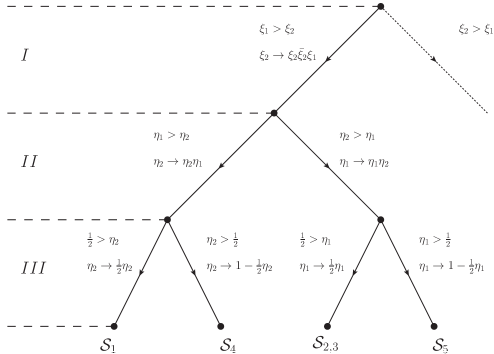
Figure 1: Decomposition tree of the triple-collinear sector unresolved phase space. The omitted right branch of the tree corresponds to a different ordering of the energies of the unresolved partons, and can be obtained by renaming the indices of the variables, $1\leftrightarrow 2$. The function $\bar{\xi}_{2}$ is defined implicitly in Eq. (11).

We consider the four sectors separately and verify the number of subtraction terms in the single-unresolved configurations

Sector 1 involves two independently vanishing variables ($\eta_{2}$ or $\xi_{2}$) in the single-unresolved kinematics, which corresponds to $u_{2}=\alpha\,r$. The relevant resolved momenta are $u_{1}$ and $r+u_{2}$ ($r/z-u_{2}$) for a final-state (initial-state) reference. $u_{1}$ is specified completely without any reference to $u_{2}$ thanks to the iterative energy parameterisation. The single-unresolved configuration is thus unique by the arguments of Section 2.1.1.

Sector 2,3 involves one vanishing variable for each of the two partons in the single-unresolved kinematics ($\eta_{1}$ for $u_{1}$, $\xi_{2}$ for $u_{2}$) implying that there are two single-unresolved configurations.

Sectors 4 and 5 involve two independently vanishing variables ($\eta_{2}$ for sector 4, $\eta_{1}$ for sector 5, or $\xi_{2}$ in both sectors) in the single-unresolved kinematics, which corresponds to $u_{2}=\alpha\,u_{1}$. The relevant resolved momenta are $r$ (if in the final state) and $u_{1}+u_{2}$. In the iterative energy parameterisation, the energy of $u_{1}+u_{2}$ depends on the energy of $u_{2}$. For this reason the single-unresolved configuration is not unique.

To make the single-unresolved configuration unique, we introduce an alternative energy parameterisation in terms of the sum of the energies and their relative proportion

$$u_{12}^{0}\equiv u_{1}^{0}+u_{2}^{0}\;,\quad\xi_{2}=\frac{2u_{2}^{0}}{(u_{1}^{0}+u_{2}^{0})}\;.$$ (13)

While $\xi_{2}\leq 2$, restricting its variation range to $\xi_{2}\in[0,\,1]$ implies $u_{1}^{0}\geq u_{2}^{0}$. For any value of $\xi_{2}$, $x$ and $z$ are monotonically decreasing functions of $u_{12}^{0}$. Let

$$\bar{u}_{12}=(1-\xi_{2}/2)\,\hat{u}_{1}+\xi_{2}/2\,\hat{u}_{2}\;.$$ (14)

For a final state reference there is

$$\big{(}u_{12}^{0}\big{)}_{\mathrm{max}}=\frac{2\,P\cdot\tilde{r}}{P\cdot\bar{u}_{12}+\sqrt{\big{(}P\cdot\bar{u}_{12}\big{)}^{2}-2\,\bar{u}_{12}^{2}\,P\cdot\tilde{r}}}\;,$$ (15)

while for an initial state reference there is

$$\big{(}u_{12}^{0}\big{)}_{\mathrm{max}}=(1-\tilde{x})\,\frac{2\,p\cdot\tilde{r}/\tilde{x}}{(\tilde{r}/\tilde{x}+p)\cdot\bar{u}_{12}+\sqrt{\big{(}(\tilde{r}/\tilde{x}+p)\cdot\bar{u}_{12}\big{)}^{2}-2\,\bar{u}_{12}^{2}\,(1-\tilde{x})\,p\cdot\tilde{r}/\tilde{x}}}\;.$$ (16)

With the energies parameterised as follows

$$u_{1}^{0}=\big{(}u_{12}^{0}\big{)}_{\mathrm{max}}\,\xi_{1}\,(1-\xi_{2}/2)\;,\quad u_{2}^{0}=\big{(}u_{12}^{0}\big{)}_{\mathrm{max}}\,\xi_{1}\,\xi_{2}/2\;,\quad\xi_{1,2}\in[0,\,1]\;,$$ (17)

the integration measure is

$$\mathrm{d}u_{1}^{0}\,\mathrm{d}u_{2}^{0}=\frac{1}{2}\,\big{(}u_{12}^{0}\big{)}_{\mathrm{max}}^{2}\,\xi_{1}\,\mathrm{d}\xi_{1}\,\mathrm{d}\xi_{2}\;.$$ (18)

If $u_{2}=\alpha\,u_{1}$, $\big{(}u_{12}^{0}\big{)}_{\mathrm{max}}$ does not depend on $u_{2}^{0}$. Thus $\xi_{1}$ uniquely determines the resolved momentum $u_{1}+u_{2}$. At the same time the rescaling of the reference momentum is also unique. In consequence, we have only one single-unresolved configuration in sector 4. There is also only one single-unresolved configuration at $\eta_{1}=0$ independently of $\xi_{2}$ in sector 5. However, there is a second single-unresolved configuration at $\xi_{2}=0$, $\eta_{1}\neq 0$ as discussed below.

The remapping of the energy variables can be introduced into the parameterisation of the phase space from the start, since the sectors 4 and 5 are defined independently of the energy of the partons. In principle, both energy parameterisations may be used in the sector 2,3. However, sector 1 requires the original parameterisation in order not to introduce additional subtraction kinematics.

Sector 5. At this point, the configurations corresponding to $\eta_{1}=0$ and $\xi_{2}=0,\eta_{1}\neq 0$ are different. This is due to the fact that the direction of the soft momentum $u_{2}$ in the latter case influences the direction of $u_{1}$ which is resolved. Thus, there is a second single-unresolved configuration.

By the above considerations, we have one single-unresolved configuration in sectors 1 and 4, and two single-unresolved configurations in sectors 2,3 and 5.

2.1.4 Two reference momenta

The following constraints allow to determine $x_{1,2}$, $z_{1,2}$ (the classification corresponds to the position of the references $r_{1}$ and $r_{2}$ in that order, $p$ is the second initial state momentum)

final-final:

$$\big{(}P-r_{1}-u_{1}-r_{2}-u_{2}\big{)}^{2}=\big{(}P-\tilde{r}_{1}-\tilde{r}_{2}\big{)}^{2}\;, \big{(}P-r_{1}-u_{1}\big{)}^{2}=\big{(}P-\tilde{r}_{1}\big{)}^{2}\;,$$

$$x_{1}=\frac{P\cdot r_{1}}{(P-u_{1})\cdot(r_{1}+u_{1})}\;, x_{2}=\frac{(P-r_{1}/x_{1})\cdot r_{2}}{(P-r_{1}-u_{1}-u_{2})\cdot(r_{2}+u_{2})}\;,$$

$$x_{1}=\frac{P\cdot(\tilde{r}_{1}-u_{1})}{(P-u_{1})\cdot\tilde{r}_{1}}\;, x_{2}=\frac{(P-\tilde{r}_{1})\cdot\tilde{r}_{2}-(P-x_{1}\tilde{r}_{1}-u_{1})\cdot u_{2}}{(P-x_{1}\tilde{r}_{1}-u_{1}-u_{2})\cdot\tilde{r}_{2}}\;,$$

$$\big{(}u_{1}^{0}\big{)}_{\mathrm{\max}}=\frac{P\cdot\tilde{r}_{1}}{P\cdot\hat{u}_{1}}\;, \big{(}u_{2}^{0}\big{)}_{\mathrm{\max}}=\frac{(P-\tilde{r}_{1})\cdot\tilde{r}_{2}}{(P-x_{1}\tilde{r}_{1}-u_{1})\cdot\hat{u}_{2}}\;,$$

$$\mathcal{J}=\frac{x_{1}^{d-3}\,P\cdot\tilde{r}_{1}}{(P-u_{1})\cdot\tilde{r}_{1}}\frac{x_{2}^{d-3}\,(P-\tilde{r}_{1})\cdot\tilde{r}_{2}}{(P-x_{1}\tilde{r}_{1}-u_{1}-u_{2})\cdot\tilde{r}_{2}}\;,$$

final-initial:

$$\big{(}p+r_{2}-r_{1}-u_{1}-u_{2}\big{)}^{2}=\big{(}p+\tilde{r}_{2}-\tilde{r}_{1}\big{)}^{2}\;, \big{(}p+\tilde{r}_{2}-r_{1}-u_{1}\big{)}^{2}=\big{(}p+\tilde{r}_{2}-\tilde{r}_{1}\big{)}^{2}\;,$$

$$z_{2}=\frac{(p-r_{1}-u_{1}-u_{2})\cdot(r_{2}-u_{2})}{(p-r_{1}-u_{1})\cdot r_{2}}\;, x_{1}=\frac{(p+z_{2}r_{2})\cdot r_{1}}{(p+z_{2}r_{2}-u_{1})\cdot(r_{1}+u_{1})}\;,$$

$$x_{1}=\frac{(p+\tilde{r}_{2})\cdot(\tilde{r}_{1}-u_{1})}{(p+\tilde{r}_{2}-u_{1})\cdot\tilde{r}_{1}}\;, z_{2}=\frac{(p-x_{1}\tilde{r}_{1}-u_{1}-u_{2})\cdot\tilde{r}_{2}}{(p-x_{1}\tilde{r}_{1}-u_{1})\cdot(\tilde{r}_{2}+u_{2})}\;,$$

$$\big{(}u_{1}^{0}\big{)}_{\mathrm{\max}}=\frac{(p+\tilde{r}_{2})\cdot\tilde{r}_{1}}{(p+\tilde{r}_{2})\cdot\hat{u}_{1}}\;, \big{(}u_{2}^{0}\big{)}_{\mathrm{\max}}=(1-\tilde{x}_{2})\frac{(p-x_{1}\tilde{r}_{1}-u_{1})\cdot\tilde{r}_{2}/\tilde{x}_{2}}{(p+\tilde{r}_{2}/\tilde{x}_{2}-x_{1}\tilde{r}_{1}-u_{1})\cdot\hat{u}_{2}}\;,$$

$$\mathcal{J}=\frac{x_{1}^{d-3}\,(p+\tilde{r}_{2})\cdot\tilde{r}_{1}}{(p+\tilde{r}_{2}-u_{1})\cdot\tilde{r}_{1}}\frac{(p-x_{1}\tilde{r}_{1}-u_{1})\cdot\tilde{r}_{2}}{(p-x_{1}\tilde{r}_{1}-u_{1}-u_{2})\cdot\tilde{r}_{2}}\;,$$

initial-final:

$$\big{(}r_{1}+p-u_{1}-r_{2}-u_{2}\big{)}^{2}=\big{(}\tilde{r}_{1}+p-\tilde{r}_{2}\big{)}^{2}\;, \big{(}r_{1}+p-u_{1}\big{)}^{2}=\big{(}\tilde{r}_{1}+p\big{)}^{2}\;,$$

$$z_{1}=\frac{(r_{1}+p)\cdot(r_{1}-u_{1})}{p\cdot r_{1}}\;, x_{2}=\frac{(z_{1}r_{1}+p)\cdot r_{2}}{(r_{1}+p-u_{1}-u_{2})\cdot(r_{2}+u_{2})}\;,$$

$$z_{1}=\frac{(p-u_{1})\cdot\tilde{r}_{1}}{p\cdot(\tilde{r}_{1}+u_{1})}\;, x_{2}=\frac{(\tilde{r}_{1}+p)\cdot\tilde{r}_{2}-(\tilde{r}_{1}/z_{1}+p-u_{1})\cdot u_{2}}{(\tilde{r}_{1}/z_{1}+p-u_{1}-u_{2})\cdot\tilde{r}_{2}}\;,$$

$$\big{(}u_{1}^{0}\big{)}_{\mathrm{\max}}=(1-\tilde{x}_{1})\frac{p\cdot\tilde{r}_{1}/\tilde{x}_{1}}{(\tilde{r}_{1}/\tilde{x}_{1}+p)\cdot\hat{u}_{1}}\;, \big{(}u_{2}^{0}\big{)}_{\mathrm{\max}}=\frac{(\tilde{r}_{1}+p)\cdot\tilde{r}_{2}}{(\tilde{r}_{1}/z_{1}+p-u_{1})\cdot\hat{u}_{2}}\;,$$

$$\mathcal{J}=\frac{p\cdot\tilde{r}_{1}}{(p-u_{1})\cdot\tilde{r}_{1}}\frac{x_{2}^{d-3}\,(\tilde{r}_{1}+p)\cdot\tilde{r}_{2}}{(\tilde{r}_{1}/z_{1}+p-u_{1}-u_{2})\cdot\tilde{r}_{2}}\;,$$

initial-initial:

$$\big{(}r_{1}+r_{2}-u_{1}-u_{2}\big{)}^{2}=\big{(}\tilde{r}_{1}+\tilde{r}_{2}\big{)}^{2}\;, \big{(}r_{1}+\tilde{r}_{2}-u_{1}\big{)}^{2}=\big{(}\tilde{r}_{1}+\tilde{r}_{2}\big{)}^{2}\;,$$

$$z_{2}=\frac{(r_{1}-u_{1}-u_{2})\cdot(r_{2}-u_{2})}{(r_{1}-u_{1})\cdot r_{2}}\;, z_{1}=\frac{(z_{2}r_{2}-u_{1})\cdot(r_{1}-u_{1})}{z_{2}r_{2}\cdot r_{1}}\;,$$

$$z_{1}=\frac{(\tilde{r}_{2}-u_{1})\cdot\tilde{r}_{1}}{\tilde{r}_{2}\cdot(\tilde{r}_{1}+u_{1})}\;, z_{2}=\frac{(\tilde{r}_{1}/z_{1}-u_{1}-u_{2})\cdot\tilde{r}_{2}}{(\tilde{r}_{1}/z_{1}-u_{1})\cdot(\tilde{r}_{2}+u_{2})}\;,$$

$$\big{(}u_{1}^{0}\big{)}_{\mathrm{\max}}=(1-\tilde{x}_{1})\frac{\tilde{r}_{2}\cdot\tilde{r}_{1}/\tilde{x}_{1}}{(\tilde{r}_{1}/\tilde{x}_{1}+\tilde{r}_{2})\cdot\hat{u}_{1}}\;, \big{(}u_{2}^{0}\big{)}_{\mathrm{\max}}=(1-\tilde{x}_{2})\frac{(\tilde{r}_{1}/z_{1}-u_{1})\cdot\tilde{r}_{2}/\tilde{x}_{2}}{(\tilde{r}_{1}/z_{1}+\tilde{r}_{2}/\tilde{x}_{2}-u_{1})\cdot\hat{u}_{2}}\;,$$

$$\mathcal{J}=\frac{\tilde{r}_{2}\cdot\tilde{r}_{1}}{(\tilde{r}_{2}-u_{1})\cdot\tilde{r}_{1}}\frac{(\tilde{r}_{1}/z_{1}-u_{1})\cdot\tilde{r}_{2}}{(\tilde{r}_{1}/z_{1}-u_{1}-u_{2})\cdot\tilde{r}_{2}}\;.$$

They have the following properties

1. the Born configuration is well defined for any full configuration, i.e. $x_{1,2},z_{1,2},\tilde{q}^{0}\geq 0$, and $x_{1}\leq 1$, $z_{1,2}\leq 1$,

2. $x_{1}$, $z_{1}$ are monotonically decreasing functions of $u_{1}^{0}$ independent of $u_{2}$,

3. $x_{2}$, $z_{2}$ are monotonically decreasing functions of $u_{2}^{0}$ at fixed $u_{1}$.

In consequence, an iterative energy parameterisation with $u_{1}^{0}$ determined in the range $\big{[}0,\,\big{(}u_{1}^{0}\big{)}_{\mathrm{max}}\big{]}$, followed by $u_{2}^{0}$ in the range $\big{[}0,\,\big{(}u_{2}^{0}\big{)}_{\mathrm{max}}(u_{1})\big{]}$ covers the full phase space. The maxima of the energies, $\big{(}u_{i}^{0}\big{)}_{\mathrm{max}}$, are obtained at $x_{i}=0$ or $z_{i}=\tilde{x}_{i}$.

Imposing an ordering of the energies, $u_{1}^{0}\geq u_{2}^{0}$, for a given phase space parameterisation is compensated by adding the contribution of the phase space for the parameterisation corresponding to swapped references. This covers the full phase space if and only if the condition $u_{1}^{0}\geq u_{2}^{0}$ is applied in the same frame in both cases. Unfortunately, if at least one of the references is in the initial state, the chosen parameterisations lead to different Born frames upon swapping the references. Therefore, the ordering of the energies cannot be imposed in the Born frame. Instead, we apply the parameterisations in a fixed frame with respect to the lab. The full phase space is then correctly covered with the energy parameterisation

$$u_{1}^{0}=\big{(}u_{1}^{0}\big{)}_{\mathrm{max}}\,\xi_{1}\;,\quad u_{2}^{0}=\big{(}u_{1}^{0}\big{)}_{\mathrm{max}}\,\xi_{1}\xi_{2}\min\Bigg{[}1,\,\frac{1}{\xi_{1}}\frac{\big{(}u_{2}^{0}\big{)}_{\mathrm{max}}}{\big{(}u_{1}^{0}\big{)}_{\mathrm{max}}}\Bigg{]}\;,\quad\xi_{1,2}\in[0,\,1]\;.$$ (19)

The parameterisation of the angles of the unresolved momenta follows Section 4.3 of Ref. Czakon:2014oma .

2.2 Reduction to four dimensions

The construction of local subtraction terms following the strategy of sector decomposition (see Ref. Czakon:2014oma for details) yields integrable expressions in CDR. The different cross section contributions are Laurent-series expansions with poles in $\epsilon$ (for the CDR parameter $d=4-2\epsilon$) whose sum is finite due to the finiteness of the (next-to-)next-to-leading order cross section. The construction in $d$ dimensions is straightforward but computationally cumbersome due to: 1) the necessity of including higher order $\epsilon$-expansion terms of matrix elements; 2) the growth with multiplicity of the number of effective dimensions of the phase space parameterisation. In Ref. Czakon:2014oma , it has been shown that a four-dimensional formulation of the subtraction scheme can be given by introducing additional corrections such that the single-unresolved ($SU$) and double-unresolved ($DU$) contributions to the next-to-next-to-leading order cross section are separately finite. In order to determine these corrections, separately finite sets of contributions must be identified. For the sake of completeness we first review the necessary notation.

The hadronic cross section is given by the collinear factorisation expression

$$\sigma_{h_{1}h_{2}}(P_{1},P_{2})=\\[5.69046pt] \sum_{ab}\iint_{0}^{1}\mathrm{d}x_{1}\mathrm{d}x_{2}\,f_{a/h_{1}}(x_{1},\mu^{2}_{F})\,f_{b/h_{2}}(x_{2},\mu^{2}_{F})\,\hat{\sigma}_{ab}(x_{1}P_{1},x_{2}P_{2};\,{\alpha_{s}}(\mu^{2}_{R}),\,\mu^{2}_{R},\,\mu^{2}_{F})\;,$$ (20)

where $P_{1,2}$ are the momenta of the hadrons $h_{1,2}$, while $p_{1,2}=x_{1,2}P_{1,2}$ are the momenta of the partons. $f_{a/h}(x,\mu^{2}_{F})$ is the PDF of parton $a$ within the hadron $h$, at the factorisation scale $\mu_{F}$. The partonic cross section can be systematically expanded in the strong coupling constant $\alpha_{s}$

$$\hat{\sigma}_{ab}=\hat{\sigma}_{ab}^{(0)}+\hat{\sigma}_{ab}^{(1)}+\hat{\sigma}_{ab}^{(2)}+\dots\;.$$ (21)

The cross sections $\hat{\sigma}_{ab}^{(i)}$ are sums of several contributions differing by the final state multiplicity, parton flavours and the number of loops of the involved matrix elements. For instance

$$\hat{\sigma}_{ab}^{(1)} =\hat{\sigma}_{ab}^{R}+\hat{\sigma}_{ab}^{V}+\hat{\sigma}_{ab}^{C}\,,$$ (22)

$$\hat{\sigma}_{ab}^{(2)} =\hat{\sigma}_{ab}^{RR}+\hat{\sigma}_{ab}^{RV}+\hat{\sigma}_{ab}^{VV}+\hat{\sigma}_{ab}^{C1}+\hat{\sigma}_{ab}^{C2}\;.$$ (23)

Here, the superscript “$R$” denotes emission of an additional parton w.r.t. to the Born final state, “$V$” denotes a virtual-loop integration, while “$C$” a convolution with Altarelli-Parisi splitting kernels. Precise definitions are given in Appendix B.

After introduction of sectors followed by the derivation of the subtraction and integrated subtraction terms, the next-to-leading order real-emission contribution is decomposed as follows

$$\hat{\sigma}^{R}=\hat{\sigma}^{R}_{F}+\hat{\sigma}^{R}_{U}\;,$$ (24)

where $\hat{\sigma}^{R}_{F}$ contains the $(n+1)$-particle tree-level matrix elements together with appropriate subtraction terms, while $\hat{\sigma}^{R}_{U}$ contains the respective integrated subtraction terms and $n$-particle tree-level matrix elements.

In general, infrared divergences can be factorised from virtual amplitudes as follows

$$|\mathcal{M}_{n}\rangle=\bm{\mathrm{Z}}(\epsilon,\{p_{i}\},\{m_{i}\},\mu_{R})\,|\mathcal{F}_{n}\rangle\;,$$ (25)

where the infrared renormalisation constant $\bm{\mathrm{Z}}$ is an operator in color space, and depends on the momenta $\{p_{i}\}=\{p_{1},...,p_{n}\}$ and masses $\{m_{i}\}=\{m_{1},...,m_{n}\}$ of the external partons. The finite remainder, $|\mathcal{F}_{n}\rangle$, has a well-defined limit when $\epsilon\rightarrow 0$. Expanding equation (25) in a series in ${\alpha_{s}}$ yields

$$|\mathcal{M}_{n}^{(0)}\rangle =|\mathcal{F}_{n}^{(0)}\rangle\;,$$ (26)

$$|\mathcal{M}_{n}^{(1)}\rangle =\bm{\mathrm{Z}}^{(1)}|\mathcal{M}_{n}^{(0)}\rangle+|\mathcal{F}_{n}^{(1)}\rangle\;,$$ (27)

$$|\mathcal{M}_{n}^{\left(2\right)}\rangle =\bm{\mathrm{Z}}^{\left(2\right)}|\mathcal{M}_{n}^{(0)}\rangle+\bm{\mathrm{Z}}^{(1)}|\mathcal{F}_{n}^{(1)}\rangle+|\mathcal{F}_{n}^{\left(2\right)}\rangle$$

$$=\left(\bm{\mathrm{Z}}^{\left(2\right)}-\bm{\mathrm{Z}}^{(1)}\bm{\mathrm{Z}}^{(1)}\right)|\mathcal{M}_{n}^{(0)}\rangle+\bm{\mathrm{Z}}^{(1)}|\mathcal{M}_{n}^{(1)}\rangle+|\mathcal{F}_{n}^{\left(2\right)}\rangle\;,$$ (28)

with $\bm{\mathrm{Z}}=\bm{1}+\bm{\mathrm{Z}}^{(1)}+\bm{\mathrm{Z}}^{(2)}+\mathcal{O}(\alpha_{s}^{3})$. This decomposition translates into a decomposition of the virtual contribution at next-to-leading order

$$\hat{\sigma}^{V}=\hat{\sigma}^{V}_{F}+\hat{\sigma}^{V}_{U}\;,$$ (29)

where $\hat{\sigma}^{V}_{F}$ contains the $n$-particle one-loop finite remainders, while $\hat{\sigma}^{V}_{U}$ contains the $n$-particle tree-level matrix elements of the $\bm{\mathrm{Z}}^{(1)}$ operator.

In consequence, there are three separately finite contributions in the next-to-leading order case

$$\hat{\sigma}^{R}_{F}\;,\quad\hat{\sigma}^{V}_{F}\;,\quad\hat{\sigma}_{U}=\hat{\sigma}^{R}_{U}+\hat{\sigma}^{V}_{U}+\hat{\sigma}^{C}\;.$$ (30)

In each separately finite contribution, it is allowed to take the $\epsilon\rightarrow 0$ limit by removing higher-order terms in the $\epsilon$-expansion of the matrix elements and reducing the dimension of the resolved momenta to four. This is the essence of the four-dimensional formulation of the subtraction scheme.

This construction can be extended to next-to-next-to-leading order, which yields the following decompositions

$$\hat{\sigma}^{RR} =\hat{\sigma}^{RR}_{F}+\hat{\sigma}^{RR}_{SU}+\hat{\sigma}^{RR}_{DU}\;,$$ (31)

$$\hat{\sigma}^{RV} =\hat{\sigma}^{RV}_{F}+\hat{\sigma}^{RV}_{SU}+\hat{\sigma}^{RV}_{FR}+\hat{\sigma}^{RV}_{DU}\;,$$ (32)

$$\hat{\sigma}^{VV} =\hat{\sigma}^{VV}_{F}+\hat{\sigma}^{VV}_{FR}+\hat{\sigma}^{VV}_{DU}\;,$$ (33)

$$\hat{\sigma}^{C1} =\hat{\sigma}^{C1}_{SU}+\hat{\sigma}^{C1}_{DU}\;,$$ (34)

$$\hat{\sigma}^{C2} =\hat{\sigma}^{C2}_{FR}+\hat{\sigma}^{C2}_{DU}\;.$$ (35)

The different contributions are identified as follows. $\hat{\sigma}^{RR,RV,VV}_{F}$ contain the same multiplicity and number-of-loops finite-remainder matrix elements as $\hat{\sigma}^{RR,RV,VV}$ together with appropriate subtraction terms to make them integrable (unnecessary for $\hat{\sigma}^{VV}$). The subscript “$FR$” (Finite Remainder) denotes the remaining contributions containing at most $n$-particle one-loop finite-remainder matrix elements. The subscript “$SU$” (Single Unresolved) denotes the remaining contributions containing at most $(n+1)$-particle tree-level matrix elements together with appropriate subtraction terms to make them integrable. Finally, the subscript “$DU$” (Double Unresolved) denotes the remaining contributions containing only $n$-particle tree-level matrix elements. The $FR$, $SU$ and $DU$ contributions contain explicit poles in $\epsilon$ due to $\bm{\mathrm{Z}}^{(1,2)}$-operator insertions and integration over subtraction terms of the $F$-contributions (and $SU$-contributions in the case of $DU$-contributions).

By construction, three contributions are separately finite

$$\hat{\sigma}^{RR}_{F}\;,\quad\hat{\sigma}^{RV}_{F}\;,\quad\hat{\sigma}^{VV}_{F}\;.$$ (36)

The finiteness of the next-to-next-to-leading order cross section implies that

$$\hat{\sigma}_{DU}+\hat{\sigma}_{SU}+\hat{\sigma}_{FR}=\text{finite}\;,$$ (37)

where

$$\hat{\sigma}_{FR} =\hat{\sigma}^{RV}_{FR}+\hat{\sigma}^{VV}_{FR}+\hat{\sigma}^{C2}_{FR}\;,$$ (38)

$$\hat{\sigma}_{SU} =\hat{\sigma}^{RR}_{SU}+\hat{\sigma}^{RV}_{SU}+\hat{\sigma}^{C1}_{SU}\;,$$

$$\hat{\sigma}_{DU} =\hat{\sigma}^{RR}_{DU}+\hat{\sigma}^{RV}_{DU}+\hat{\sigma}^{C1}_{DU}+\hat{\sigma}^{VV}_{DU}+\hat{\sigma}^{C2}_{DU}\;.$$

Following the argument of Ref. Czakon:2014oma , $\hat{\sigma}_{FR}$ is separately finite due to the finiteness of the next-to-leading order cross section. Indeed, $\hat{\sigma}_{FR}$ is given by the same expressions as $\hat{\sigma}_{U}$ once tree-level amplitudes are replaced by one-loop finite remainders in the latter. This leaves $\hat{\sigma}_{DU}+\hat{\sigma}_{SU}$ to be finite.

Unfortunately, it turns out that $\hat{\sigma}_{DU}$ and $\hat{\sigma}_{SU}$ are both separately divergent despite having different multiplicity resolved final states. A four-dimensional formulation of the subtraction scheme is only obtained under the assumption that a $\hat{\sigma}_{HV}$, the ’t Hooft-Veltman corrections contribution, linear in the infrared safe measurement function $F_{n}$ exists such that

$$\tilde{\sigma}_{SU} =\hat{\sigma}_{SU}-\hat{\sigma}_{HV}\;,$$ (39)

$$\tilde{\sigma}_{DU} =\hat{\sigma}_{DU}+\hat{\sigma}_{HV}\;,$$ (40)

are separately finite. An appropriate $\hat{\sigma}_{HV}$ has been constructed in Ref. Czakon:2014oma . Here, we present a different construction which exploits the fact that $\hat{\sigma}_{SU}$ is finite for a next-to-leading order measurement function, i.e. for $F_{n}=0$. The approach relies on the idea that, since the cut on the additional radiation in $F_{n+1}$ is arbitrary, the divergences in $\hat{\sigma}_{SU}$ with a next-to-next-to-leading order measurement function, i.e. for $F_{n}\neq 0$, can, in fact, be described with $n$-particle kinematics and matrix elements. It should thus be possible to systematically identify them and subsequently shift them to $\hat{\sigma}_{DU}$.

2.2.1 ’t Hooft-Veltman corrections

The replacement of the next-to-next-to-leading order measurement function with a next-to-leading order measurement function, i.e. one with $F_{n+1}\neq 0$ and $F_{n}=0$, turns $\hat{\sigma}_{SU}$ into the $\hat{\sigma}_{U}$ of an $(n+1)$-particle next-to-leading order cross section with

$$\hat{\sigma}^{RU}_{SU}\;\to\;\hat{\sigma}^{R}_{U}\;,\quad\hat{\sigma}^{RV}_{SU}\;\to\;\hat{\sigma}^{V}_{U}\;,\quad\hat{\sigma}^{C1}_{SU}\;\to\;\hat{\sigma}^{C}\,.$$ (41)

At next-to-leading order, the contributions $\hat{\sigma}^{R}_{U}$, $\hat{\sigma}^{V}_{U}$ and $\hat{\sigma}^{C}$ may be written in the following form

$$\hat{\sigma}^{R}_{U} =\int\differential\Phi^{(d)}_{n+1}\;\mathcal{I}^{R}_{n+1}F_{n+1}\;,$$ (42)

$$\hat{\sigma}^{V}_{U} =\int\differential\Phi^{(d)}_{n+1}\;\mathcal{I}^{V}_{n+1}F_{n+1}\;,$$ (43)

$$\hat{\sigma}^{C} =\int\differential\Phi^{(d)}_{n+1}\;\mathcal{I}^{C}_{n+1}F_{n+1}\;.$$ (44)

Notice that $\mathcal{I}^{R}_{n+1}$ is given by a sum of contributions of individual sectors, which makes the factorisation of the $d$-dimensional phase space measure $\differential\Phi^{(d)}_{n+1}$ non-trivial. With the phase space parameterisations of Section 2.1, this factorisation can, nevertheless, be achieved explicitly in each sector.

Let us now consider the structure of the $\epsilon$-expansions of the integrands $\mathcal{I}^{c}_{n+1}$, $c\in\{R,V,C\}$, while keeping the exact $\epsilon$-dependence of the occurring matrix elements. We have

$$\mathcal{I}^{R}_{n+1} =\frac{\mathcal{I}^{R(-2)}_{n+1}}{\epsilon^{2}}+\frac{\mathcal{I}^{R(-1)}_{n+1}}{\epsilon}+\mathcal{I}^{R(0)}_{n+1}+\order{\epsilon}\;,$$ (45)

$$\mathcal{I}^{V}_{n+1} =\frac{\mathcal{I}^{V(-2)}_{n+1}}{\epsilon^{2}}+\frac{\mathcal{I}^{V(-1)}_{n+1}}{\epsilon}\;,$$ (46)

$$\mathcal{I}^{C}_{n+1} =\frac{\mathcal{I}^{C(-1)}_{n+1}}{\epsilon}+\mathcal{I}^{C(0)}_{n+1}+\order{\epsilon}\;,$$ (47)

where each $\mathcal{I}^{c(i)}_{n+1}$ is a function of $\epsilon$ through the $\epsilon$-dependence of the tree-level matrix elements only. The simple structure of $\mathcal{I}^{V}_{n+1}$ is due to the fact that it is given by matrix elements of the $\mathbf{Z}^{(1)}$-operator which we chose to be defined in the $\overline{\mathrm{MS}}$ scheme, where it consists of pure poles. Even though collinear factorisation is also performed in the $\overline{\mathrm{MS}}$ scheme, $\mathcal{I}^{C}_{n+1}$ does have a non-trivial $\epsilon$-expansion for $\mu_{R}\neq\mu_{F}$ because of the expansion of the pre-factor $(\mu_{R}^{2}/\mu_{F}^{2})^{\epsilon}$ in (64). The finiteness of the next-to-leading order cross section implies

$$\sum_{c}\int\differential\Phi^{(d)}_{n+1}\left[\frac{\mathcal{I}^{c(-2)}_{n+1}}{\epsilon^{2}}+\frac{\mathcal{I}^{c(-1)}_{n+1}}{\epsilon}\right]F_{n+1}\equiv\sum_{c}\mathcal{I}^{c}=0\;.$$ (48)

This analysis translates directly to $\hat{\sigma}_{SU}$ with an appropriate change of superscripts.

Parameterised measurement function.

Let us introduce a family of measurement functions $F^{\alpha}_{m}$, $m\in\{n,n+1,n+2\}$ with the following properties

• $F^{\alpha}_{m}$ is infrared safe;

• $F^{\alpha\neq 0}_{n}=0$ and $F^{\alpha=0}_{n}\neq 0$.

Hence, $\alpha\neq 0$ corresponds to a next-to-leading order calculation within a next-to-next-to-leading order setup, while $\alpha=0$ corresponds to the general next-to-next-to-leading order calculation. Since we only consider single- and double-unresolved contributions, it is not necessary to define $F^{\alpha}_{n+2}$. In order to identify the ’t Hooft-Veltman corrections, a particularly useful realisation is given by

$$F^{\alpha}_{n+1}=F_{n+1}\theta(\alpha_{\eta}-\alpha)\theta(\alpha_{\xi}-\alpha)\equiv F_{n+1}\theta_{\eta}\theta_{\xi}\equiv F_{n+1}\theta_{\alpha}\;,$$ (49)

with $F^{\alpha}_{n}$ obtained from $F^{\alpha}_{n+1}$ by taking soft and/or collinear limits. $\alpha_{\eta}$ and $\alpha_{\xi}$ are a set of global infrared sensitive variables

$$\alpha_{\eta}=\min_{ij}\eta_{ij}\;, \eta_{ij}=\frac{1}{2}\left(1-\cos\theta_{ij}\right)\;,$$ with (50)

$$\alpha_{\xi}=\min_{i}\xi_{i}\;, \xi_{i}=\frac{p_{i}^{0}}{E_{\text{norm}}}\;,$$ with (51)

where $\theta_{ij}$ is the angle between two parton momenta, and $p_{i}^{0}$ is a parton energy. The variable $\alpha_{\eta}$ measures the minimal angle between any two partons $i$ and $j$, while $\alpha_{\xi}$ measures the minimal energy of the partons with respect to some arbitrary energy scale $E_{\text{norm}}$. For $\alpha\neq 0$, $F^{\alpha}_{m}$ is a well-defined next-to-leading order measurement function. For $\alpha=0$, it corresponds to the original next-to-next-to-leading order measurement function.

Identification of ’t Hooft-Veltman corrections.

Using the parameterised measurement function, the next-to-next-to-leading order version of Eq. (48) takes the form

$$\sum_{c}\int\differential\Phi^{(d)}_{n+1}\;\left[\frac{\mathcal{I}^{c(-2)}_{n+1}}{\epsilon^{2}}+\frac{\mathcal{I}^{c(-1)}_{n+1}}{\epsilon}\right]F^{\alpha\neq 0}_{n+1}\equiv\sum_{c}\mathcal{I}^{c}=0\;,$$ (52)

with $c\in\{RR,RV,C1\}$. Considering the full next-to-next-to-leading order case, we can schematically write the contributions $\hat{\sigma}^{c}_{SU}$ in the following form

$$\hat{\sigma}^{c}_{SU} =\int\differential\Phi^{(d)}_{n+1}\left[\mathcal{I}^{c}_{n+1}F_{n+1}+\mathcal{I}^{c}_{n}F_{n}\right]$$ (53)

$$=\int\differential\Phi^{(d)}_{n+1}\left\{\left[\frac{\mathcal{I}^{c(-2)}_{n+1}}{\epsilon^{2}}+\frac{\mathcal{I}^{c(-1)}_{n+1}}{\epsilon}+\mathcal{I}^{c(0)}_{n+1}\right]F_{n+1}+\left[\frac{\mathcal{I}^{c(-2)}_{n}}{\epsilon^{2}}+\frac{\mathcal{I}^{c(-1)}_{n}}{\epsilon}+\mathcal{I}^{c(0)}_{n}\right]F_{n}\right\}$$

$$\quad+\order{\epsilon}\;.$$ (54)

The integrands $\mathcal{I}^{c}_{n}=\sum\limits_{i=-2}^{\infty}\mathcal{I}^{c(i)}_{n}$ represent the subtraction terms that regulate the $n$-particle limit of $\mathcal{I}^{c}_{n+1}$. Here, following the discussion of the next-to-leading order case, $\mathcal{I}^{c(i)}_{n+1}$ contain the unexpanded $(n+1)$-particle matrix elements. Hence, $\mathcal{I}^{c(i)}_{n}$ consist of the appropriate unexpanded factorisation formulae for $(n+1)$-particle matrix elements in the single-soft and collinear limits.

Consider now the difference $\hat{\sigma}^{c}_{SU}-\mathcal{I}^{c}$. By reshuffling terms and neglecting $\mathcal{O}(\epsilon)$ contributions, it can be written as

$$\hat{\sigma}^{c}_{SU}-\mathcal{I}^{c} =\int\differential\Phi^{(d)}_{n+1}\left[\frac{\mathcal{I}^{c(-2)}_{n+1}F_{n+1}+\mathcal{I}^{c(-2)}_{n}F_{n}}{\epsilon^{2}}+\frac{\mathcal{I}^{c(-1)}_{n+1}F_{n+1}+\mathcal{I}^{c(-1)}_{n}F_{n}}{\epsilon}\right]\left(1-\theta_{\alpha}\right)$$

$$+\int\differential\Phi^{(d)}_{n+1}\left[\mathcal{I}^{c(0)}_{n+1}F_{n+1}+\mathcal{I}^{c(0)}_{n}F_{n}\right]+\int\differential\Phi^{(d)}_{n+1}\left[\frac{\mathcal{I}^{c(-2)}_{n}}{\epsilon^{2}}+\frac{\mathcal{I}^{c(-1)}_{n}}{\epsilon}\right]F_{n}\theta_{\alpha}$$

$$\equiv Z^{c}(\alpha)+C^{c}+N^{c}(\alpha)\;.$$ (55)

The integral $C^{c}$ neither depends on the parameter $\alpha$ nor contains poles in $\epsilon$. The integrand of $Z^{c}(\alpha)$ is integrable while the phase space volume is restricted by $1-\theta_{\alpha}$. The phase space volume thus vanishes in the $\alpha\to 0$ limit and so does $Z^{c}(\alpha)$. Finally, the phase space integral in

$$N^{c}(\alpha)=\int\differential\Phi^{(d)}_{n+1}\left[\frac{\mathcal{I}^{c(-2)}_{n}}{\epsilon^{2}}+\frac{\mathcal{I}^{c(-1)}_{n}}{\epsilon}\right]F_{n}\theta_{\alpha}\;,$$ (56)

contains integrations over the angle and energy variables which might give rise to singularities regulated by $\alpha$. In particular, after sector decomposition, the only singularities in a given phase space sector are due to soft and collinear limits of the unresolved parton momenta. In consequence, we can safely take the limit $\alpha\to 0$, if neither $\alpha_{\eta}$ nor $\alpha_{\xi}$ correspond to unresolved partons. Hence, the general contribution to $N^{c}(\alpha)$ contains terms regular at $\alpha\to 0$ and integrals of the form

$$\begin{split}\int_{0}^{1}\frac{\differential x}{x^{1+a\epsilon}}&\theta(x-f(x)\alpha)\\[5.69046pt] &=\int_{0}^{1}\frac{\differential x}{x^{1+a\epsilon}}\theta(x-f(0)\alpha)+\int_{0}^{1}\frac{\differential x}{x^{1+a\epsilon}}\left(\theta(x-f(x)\alpha)-\theta(x-f(0)\alpha)\right)\\[5.69046pt] &=\int_{0}^{1}\frac{\differential x}{x^{1+a\epsilon}}\theta(x-f(0)\alpha)+\order{\alpha}\\[5.69046pt] &=-\frac{1-(f(0)\alpha)^{-a\epsilon}}{a\epsilon}+\order{\alpha}\;,\end{split}$$ (57)

where $x$ is one of $\eta_{1}$, $\eta_{2}$, $\xi_{1}$, $\xi_{2}$. Expansion in $\epsilon$ yields the power-log series

$$N^{c}(\alpha)=\sum_{k=0}^{l_{\text{max}}}\ln^{k}(\alpha)N^{c}_{k}(\alpha)\;,$$ (58)

where $N^{c}_{k}(\alpha)$ are regular at $\alpha\to 0$.

The modified $SU$ contributions are used as follows

$$\hat{\sigma}_{SU}=\hat{\sigma}_{SU}-\underbrace{\sum_{c}\mathcal{I}^{c}}_{=0}=\sum_{c}\left(\hat{\sigma}^{c}_{SU}-\mathcal{I}^{c}\right)=\sum_{c}\left(Z^{c}(\alpha)+C^{c}+N^{c}(\alpha)\right)\;.$$ (59)

The left-hand side is independent of $\alpha$ and, therefore, the right-hand side has to be independent as well. Since $Z^{c}(\alpha)$ are regular functions of $\alpha$ which vanish in the limit $\alpha\to 0$, the logarithms appearing in (58) have to cancel across the different contributions $c$. In the limit $\alpha\to 0$, we thus find that the poles that do not cancel within $\hat{\sigma}_{SU}$ are given by

$$\sum_{c}N^{c}_{0}(0)\equiv\hat{\sigma}_{HV}\;.$$ (60)

Thus, subtracting $\hat{\sigma}_{HV}$ from $\hat{\sigma}_{SU}$ yields a finite quantity where all poles cancel. Since all terms in $\hat{\sigma}_{HV}$ are proportional to $F_{n}$, $\hat{\sigma}_{HV}$ can be added to $\hat{\sigma}_{DU}$. By the finiteness of the next-to-next-to-leading order cross section it follows that

$$\tilde{\sigma}_{SU}=\hat{\sigma}_{SU}-\hat{\sigma}_{HV}\;,\quad\text{and}\quad\tilde{\sigma}_{DU}=\hat{\sigma}_{DU}+\hat{\sigma}_{HV}\;,$$ (61)

are separately finite.

The formal manipulations of the different contributions must be performed in $d$ dimensions. However, after this procedure, the ’t Hooft-Veltman regularisation discussed in Section 8 of Ref. Czakon:2014oma can be applied yielding the desired four-dimensional formulation of the subtraction scheme. A collection of the required ’t Hooft-Veltman corrections can be found in Appendix C.

2.3 Implementation and tests

We have implemented the complete subtraction scheme in the C++ library Stripper. In principle, the library provides sufficient functionality to evaluate NNLO QCD corrections to any process in the Standard Model. In practice, it requires appropriate matrix elements at tree-level (including up to double correlations in color and/or spin), one-loop level (including single correlations in color or spin), and two-loop level. Tree-level matrix elements for arbitrary Standard Model processes are provided by default by the Fortran library avhlib introduced in Ref. Bury:2015dla . The code generates amplitudes on-the-fly for arbitrary polarisations (helicities) and color configurations of external states and evaluates them numerically in double precision. We note that, while completely general, this is slower than dedicated analytic expressions for parton-scattering processes at low multiplicity. The five-point one-loop matrix element values that were required for our computation of jet rates have been obtained using the NJet C++ library presented in Refs. Badger:2010nx ; Badger:2012pg . However, the general numerical-unitarity algorithm implemented in the library turned out to be too slow and unstable for our purposes. Instead, we have used the analytic formulae Bern:1993mq ; Bern:1994fz ; Kunszt:1994nq for five-parton matrix elements implemented in NJet. The two-loop amplitudes have been taken from Ref. Broggio:2014hoa , which is based on Refs. Glover:2003cm ; Glover:2004si ; Bern:2003ck ; DeFreitas:2004kmi ; Bern:2002tk .

The correctness of the results obtained with Stripper depends on the correctness of the matrix elements, splitting and soft functions, $d$-dimensional and four-dimensional phase spaces, and, finally, the ’t Hooft-Veltman corrections. Apart from matrix elements, the majority of these contributions is involved in the evaluation of the NNLO QCD corrections to hadronic top-quark pair production. With the new implementation, we were able to reproduce the results of Refs. Czakon:2015owf ; Czakon:2016dgf , which have recently been confirmed in Ref. Catani:2019hip . On the other hand, our most recent results Behring:2019iiv for this process including Narrow-Width-Approximation top-quark decays in the di-lepton channel have only been obtained with the new version of Stripper.

A final test of the phase space implementation and the ’t Hooft-Veltman corrections has been performed by calculating the single-jet inclusive double-differential ($p_{T}$, $|y|$) cross section in the pure-gluon channel for proton-proton collisions at 7 TeV center-of-mass energy, jets defined with the anti-$k_{T}$ algorithm with $R=0.7$ and with the scale $\mu_{R}=\mu_{F}=\mu=p_{T,1}/2,p_{T,1},2p_{T,1}$ for the MMHT2014nnlo68cl PDF set. In this case, we have found perfect agreement within the statistical errors estimated at below 1% with results obtained with NNLOjet (private communication). This test covers all aspects of our software necessary for the evaluation of the cross sections in the remaining channels involving quarks.

3 Single-jet inclusive rates for LHC @ 13 TeV

In this section, we present our results for the single-jet inclusive differential distributions in the jet transverse momentum ($p_{T}$) in several jet rapidity ($|y|$) slices. We assume an initial state corresponding to proton-proton collisions at 13 TeV center-of-mass energy and use the central PDF4LHC15_nnlo PDF set to obtain the parton densities. The strong coupling constant running corresponds to this PDF set as well. Jets are identified with the anti-$k_{T}$ jet algorithm with $R=0.7$, $p_{T}>114$ GeV and $|y|<4.7$. Every jet identified in a given final-state parton configuration (event) is input into the appropriate rapidity-slice histogram with a weight that corresponds to a cross section contribution evaluated with the scale $\mu_{R}=\mu_{F}=\mu\in\{p_{T},2p_{T},4p_{T}\}$. The weight corresponding to $\mu=2p_{T}$ is taken as the central value of the prediction, while the remaining values are used to estimate the scale uncertainty.

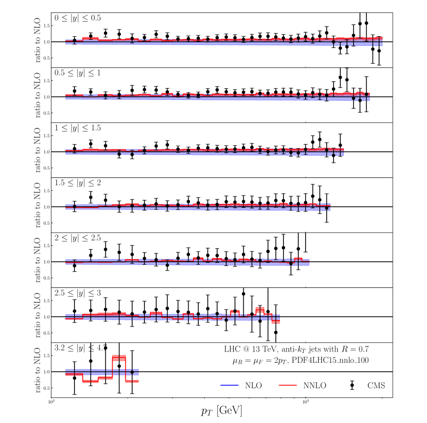
Figure 2: Double-differential single jet inclusive cross-sections as measured by CMS Khachatryan:2016wdh and NNLO perturbative QCD predictions as a function of the jet $p_{T}$ in slices of rapidity, for anti-$k_{T}$ jets with R = 0.7 normalised to the NLO result. Both perturbative predictions, NLO and NNLO, have been obtained with the PDF4LHC15_nnlo PDF set and with $\mu_{R}=\mu_{F}=2p_{T}$. The shaded bands represent the scale uncertainty obtained from differential distributions evaluated at $\mu_{R}=\mu_{F}=p_{T}$ and $\mu_{R}=\mu_{F}=4p_{T}$.

In Fig. 2 we compare the NNLO QCD results with the experimental measurement values from Ref. Khachatryan:2016wdh . Results are normalised to the NLO QCD prediction. The scale uncertainty of the latter is also shown. We do not include non-perturbative or electroweak corrections. It is expected that the non-perturbative effects are smaller for $R=0.4$ than for $R=0.7$. However, we are not interested in having the most complete prediction, and thus choose somewhat arbitrarily one of the $R$ values. Furthermore, with the current experimental precision, neither non-perturbative nor electroweak effects are necessary to obtain a good description of the data.

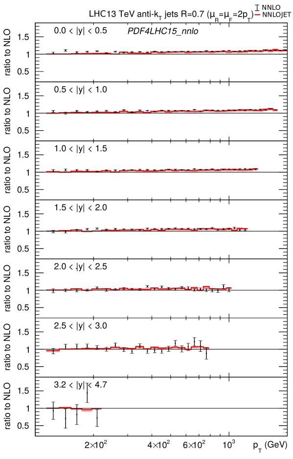
Figure 3: Comparison of the cross section ratios depicted in Fig. 2 as obtained with NNLOjet Currie:2018xkj (red line with scale variation error, leading-color approximation for channels involving quarks) and with Stripper (black points with Monte Carlo integration error bars, as given in Appendix D, exact in color). This figure has been obtained from Fig. 21 of Currie:2018xkj by removing the experimental data points as well as the scale variation band of the NLO calculation, followed by superimposing the results obtained in the present work.

In Fig. 3, we compare our results with those obtained with NNLOjet as presented in Ref. Currie:2018xkj . Since no numerical values are given in the latter publication, we superimpose our values, including the estimated Monte Carlo integration error as listed in Appendix D, on the respective plot from Ref. Currie:2018xkj . The results appear to be compatible within their respective errors. The largest significant differences are observed in the first rapidity slice at low jet transverse momenta. However, this is the phase space region, where pure-gluon contributions dominate. The latter have been compared separately (see Section 2.3) and agree within one percent. We also note that even though the bulk of the events are in the low-$p_{T}$/central-rapidity region, our calculation is not optimised to yield very small integration errors there. More interesting is the comparison of the results for higher $p_{T}$ and in the first four rapidity slices ($|y|<2.0$). There, our calculation has an estimated integration error at the level of about one percent, and is still compatible with the NNLOjet result. This implies that sub-leading color effects missing in the contributions of channels involving quarks in NNLOjet are indeed at most at this level. The integration errors of our calculation in the fifth rapidity slice ($2.0<|y|<2.5$) are still less than about five percent and the two calculations remain compatible, although NNLOjet results are clearly more precise. While the integration errors in the sixth rapidity slice ($2.5<|y|<3.0$) remain below ten percent, the results can hardly be used as a precise indicator of sub-leading color effects. We also provide the outcome of our calculation in the last rapidity slice ($3.2<|y|<4.7$) to illustrate the limits of reasonable convergence within our setup.

Let us finally comment on the convergence of the Monte Carlo integration in Stripper for this process. The results presented in Figs. 2 and 3 required about 350000 CPU hours. In particular, $\hat{\sigma}^{RR}_{F}$ was evaluated with 200000 CPU hours, $\hat{\sigma}_{SU}$ with 100000 CPU hours and $\hat{\sigma}_{DU}$ with 50000 CPU hours. A further improvement of the integration errors would require doubling the evaluation time for $\hat{\sigma}_{SU}$. It is important to note that the computation cost of the integrated subtraction terms present in $\hat{\sigma}_{DU}$ and $\hat{\sigma}_{SU}$ is still less than that of the pure real radiation. Hence, even if one could reduce it substantially by performing analytic integrations of the subtraction terms, the calculation would be at most twice faster for the same quality of the results. To put the performance into perspective, we point out that results for typical top-quark distributions as published recently require less than a twentieth of the quoted running times.

4 Outlook

In the present publication, we have performed a first independent and also the first complete calculation of single-jet inclusive rates for LHC @ 13 TeV with NNLO QCD accuracy. After comparing with results obtained with NNLOjet, we concluded that the sub-leading color effects not included in NNLOjet are negligible for phenomenological applications of the studied observable. One obvious extension of the present work is to evaluate fastNLO and/or APPLGRID tables for all measured jet observables in order to allow for inclusion of the experimental data in PDF fits. In view of the current computational costs, this requires either a substantial improvement of the efficiency of Stripper or the acquisition of substantial computational resources.

Apart from the calculation of jet rates, we have also discussed a further evolution of the sector-improved residue subtraction scheme which allows for a minimal number of subtraction terms per phase space point. This approach does improve the convergence of cross sections, but to quantify the improvement requires further studies. There are still several avenues to explore in order to optimise the subtraction scheme. They range from pure Monte Carlo techniques such as better sampling of the initial state, through speed-ups of matrix element evaluation by using analytic formulae, and finishing with further modifications of the phase space treatment. We hope to be able to substantially reduce the cost of calculations in the future.

Appendix A Previous theoretical predictions for jet rates at NNLO in QCD

Single-jet inclusive cross sections

1. Ref. Currie:2016bfm corresponding to 7 TeV ATLAS data presented in Ref. Aad:2014vwa

   • jets defined with the anti-$k_{T}$ jet algorithm with $R=0.4$, $p_{T}>100$ GeV and $|y|<3.0$;

   • hardest-jet scale: $\mu_{R}=\mu_{F}=\mu=p_{T,1}$.

2. Ref. Currie:2018xkj corresponding to 13 TeV CMS data presented in Ref. Khachatryan:2016wdh (available on HEPDATA https://www.hepdata.net/record/ins1459051)

   • jets defined with the anti-$k_{T}$ jet algorithm with $R=0.4$ and $R=0.7$, $p_{T}>114$ GeV and $|y|<4.7$;

   • various scales: $\mu_{R}=\mu_{F}=\mu=p_{T,1},\hat{H}_{T},2p_{T}$.

Di-jet cross sections

1. Ref. Currie:2017eqf corresponding to 7 TeV ATLAS data presented in Ref. Aad:2013tea (available on HEPDATA https://www.hepdata.net/record/ins1268975)

   • at least two jets identified with the anti-$k_{T}$ jet algorithm with $R=0.4$, $p_{T}>100(50)$ GeV for the leading (sub-leading) jet and $|y|<3.0$;

   • scale: $\mu=m_{jj}$ and $\mu=\langle p_{T}\rangle=(p_{T_{1}}+p_{T_{2}})/2$ (at NNLO both scales show similar behaviour);

   • double-differential distributions ($m_{jj}$, $|y^{*}|$);

   • includes electroweak corrections from Ref. Dittmaier:2012kx .

2. Ref. Gehrmann-DeRidder:2019ibf corresponding to 8 TeV CMS data presented in Ref. Sirunyan:2017skj (available on HEPDATA https://www.hepdata.net/record/ins1598460)

   • at least two jets identified with the anti-$k_{T}$ jet algorithm with $R=0.7$, $p_{T}>50$ GeV and $|y|<3.0$;

   • scale: $\mu=m_{jj}$;

   • triple-differential distributions ($p_{T,\mathrm{avg}}$, $|y^{*}|$, $y_{b}$) in six $(y^{*},y_{b})$ regions (binning available from HEPDATA);

   • includes non-perturbative and electroweak effects as multiplicative factors (bin-wise, available from HEPDATA).

Appendix B Cross section contributions

At leading order

$$\hat{\sigma}^{(0)}_{ab}=\hat{\sigma}^{{B}}_{ab}=\frac{1}{2\hat{s}}\frac{1}{N_{ab}}\int\mathrm{d}\bm{\Phi}_{n}\,\langle\mathcal{M}_{n}^{(0)}|\mathcal{M}_{n}^{(0)}\rangle\,F_{n}\;,$$ (62)

where $\hat{s}=(p_{1}+p_{2})^{2}$ is the square of the partonic center-of-mass energy, while $N_{ab}$ is the spin and color average factor, defined as the product of the number of spin and color degrees of freedom of the partons $a$ and $b$. The subscript $n$ points to the number of final states in this contribution and $\mathrm{d}\bm{\Phi}_{n}$ is the phase space measure for $n$ particles. $F_{n}$ is the infrared-safe measurement function defining the observable. Here and below, $|\mathcal{M}_{n}^{(l)}\rangle$ are $l$-loop amplitudes for $n$ particles understood as vectors in color and spin space. At next-to-leading order there is

$$\hat{\sigma}^{(1)}_{ab}=\hat{\sigma}^{{R}}_{ab}+\hat{\sigma}^{{V}}_{ab}+\hat{\sigma}^{{C}}_{ab}\;,$$ (63)

with

$$\hat{\sigma}^{{R}}_{ab} =\frac{1}{2\hat{s}}\frac{1}{N_{ab}}\int\mathrm{d}\bm{\Phi}_{n+1}\,\langle\mathcal{M}_{n+1}^{(0)}|\mathcal{M}_{n+1}^{(0)}\rangle\,F_{n+1}\;,$$ (64)

$$\hat{\sigma}^{{V}}_{ab} =\frac{1}{2\hat{s}}\frac{1}{N_{ab}}\int\mathrm{d}\bm{\Phi}_{n}\,2\mathrm{Re}\,\langle\mathcal{M}_{n}^{(0)}|\mathcal{M}_{n}^{(1)}\rangle\,F_{n}\;,$$

$$\hat{\sigma}^{{C}}_{ab}(p_{1},p_{2}) =\frac{{\alpha_{s}}}{2\pi}\frac{1}{\epsilon}\left(\frac{\mu^{2}_{R}}{\mu^{2}_{F}}\right)^{\epsilon}\sum_{c}\int_{0}^{1}\mathrm{d}z\left[P^{(0)}_{ca}(z)\,\hat{\sigma}^{{B}}_{cb}(zp_{1},p_{2})+P^{(0)}_{cb}(z)\,\hat{\sigma}^{{B}}_{ac}(p_{1},zp_{2})\right]\;,$$

where $P^{(l)}_{ab}$ are Altarelli-Parisi splitting kernels at order $l$. Finally, at next-to-next-to-leading order, we have

$$\hat{\sigma}^{(2)}_{ab}=\hat{\sigma}^{{RR}}_{ab}+\hat{\sigma}^{{RV}}_{ab}+\hat{\sigma}^{{VV}}_{ab}+\hat{\sigma}^{{C1}}_{ab}+\hat{\sigma}^{{C2}}_{ab}\;,$$ (65)

with

$$\hat{\sigma}^{{RR}}_{ab} =\frac{1}{2\hat{s}}\frac{1}{N_{ab}}\int\mathrm{d}\bm{\Phi}_{n+2}\,\langle\mathcal{M}_{n+2}^{(0)}|\mathcal{M}_{n+2}^{(0)}\rangle\,F_{n+2}\;,$$ (66)

$$\hat{\sigma}^{{RV}}_{ab} =\frac{1}{2\hat{s}}\frac{1}{N_{ab}}\int\mathrm{d}\bm{\Phi}_{n+1}\,2\mathrm{Re}\,\langle\mathcal{M}_{n+1}^{(0)}|\mathcal{M}_{n+1}^{(1)}\rangle\,F_{n+1}\;,$$

$$\hat{\sigma}^{{VV}}_{ab} =\frac{1}{2\hat{s}}\frac{1}{N_{ab}}\int\mathrm{d}\bm{\Phi}_{n}\,\Big{(}2\mathrm{Re}\,\langle\mathcal{M}_{n}^{(0)}|\mathcal{M}_{n}^{(2)}\rangle+\langle\mathcal{M}_{n}^{(1)}|\mathcal{M}_{n}^{(1)}\rangle\Big{)}\,F_{n}\;,$$

and

$$\begin{split}\hat{\sigma}^{{C1}}_{ab}(p_{1},p_{2})&=\frac{{\alpha_{s}}}{2\pi}\frac{1}{\epsilon}\left(\frac{\mu^{2}_{R}}{\mu^{2}_{F}}\right)^{\epsilon}\sum_{c}\int_{0}^{1}\mathrm{d}z\left[P^{(0)}_{ca}(z)\,\hat{\sigma}^{{R}}_{cb}(zp_{1},p_{2})+P^{(0)}_{cb}(z)\,\hat{\sigma}^{{R}}_{ac}(p_{1},zp_{2})\right]\;,\\[5.69046pt] \hat{\sigma}^{{C2}}_{ab}(p_{1},p_{2})&=\frac{{\alpha_{s}}}{2\pi}\frac{1}{\epsilon}\left(\frac{\mu^{2}_{R}}{\mu^{2}_{F}}\right)^{\epsilon}\sum_{c}\int_{0}^{1}\mathrm{d}z\left[P^{(0)}_{ca}(z)\,\hat{\sigma}^{{V}}_{cb}(zp_{1},p_{2})+P^{(0)}_{cb}(z)\,\hat{\sigma}^{{V}}_{ac}(p_{1},zp_{2})\right]\\ &+\left(\frac{{\alpha_{s}}}{2\pi}\right)^{2}\frac{1}{2\epsilon}\left(\frac{\mu^{2}_{R}}{\mu^{2}_{F}}\right)^{2\epsilon}\sum_{c}\int_{0}^{1}\mathrm{d}z\left[P^{(1)}_{ca}(z)\,\hat{\sigma}^{{B}}_{cb}(zp_{1},p_{2})+P^{(1)}_{cb}(z)\,\hat{\sigma}^{{B}}_{ac}(p_{1},zp_{2})\right]\\ &+\left(\frac{{\alpha_{s}}}{2\pi}\right)^{2}\frac{\beta_{0}}{4\epsilon^{2}}\left[\left(\frac{\mu^{2}_{R}}{\mu^{2}_{F}}\right)^{2\epsilon}-2\left(\frac{\mu^{2}_{R}}{\mu^{2}_{F}}\right)^{\epsilon}\right]\sum_{c}\int_{0}^{1}\mathrm{d}z\left[P^{(0)}_{ca}(z)\,\hat{\sigma}^{{B}}_{cb}(zp_{1},p_{2})+P^{(0)}_{cb}(z)\,\hat{\sigma}^{{B}}_{ac}(p_{1},zp_{2})\right]\\ &+\left(\frac{{\alpha_{s}}}{2\pi}\right)^{2}\frac{1}{2\epsilon^{2}}\left(\frac{\mu^{2}_{R}}{\mu^{2}_{F}}\right)^{2\epsilon}\sum_{cd}\int_{0}^{1}\mathrm{d}z\left[\Big{(}P^{(0)}_{cd}\otimes P^{(0)}_{da}\Big{)}(z)\,\hat{\sigma}^{{B}}_{cb}(zp_{1},p_{2})+\Big{(}P^{(0)}_{cd}\otimes P^{(0)}_{db}\Big{)}(z)\,\hat{\sigma}^{{B}}_{ac}(p_{1},zp_{2})\right]\\ &+\left(\frac{{\alpha_{s}}}{2\pi}\right)^{2}\frac{1}{\epsilon^{2}}\left(\frac{\mu^{2}_{R}}{\mu^{2}_{F}}\right)^{2\epsilon}\sum_{cd}\iint_{0}^{1}\mathrm{d}z\,\mathrm{d}\bar{z}\left[P^{(0)}_{ca}(z)\,P^{(0)}_{db}({\bar{z}})\,\hat{\sigma}^{{B}}_{cd}(zp_{1},\bar{z}p_{2})\right]\;,\end{split}$$ (67)

where

$$\left(f\otimes g\right)(x)=\iint_{0}^{1}\mathrm{d}y\,\mathrm{d}z\,f(y)g(z)\,\delta(x-yz)\;.$$ (68)

Appendix C ’t Hooft-Veltman corrections

Double-real contributions

The ’t Hooft-Veltman corrections to double-pole contributions contained in $\mathcal{S}_{1}$, $\mathcal{S}_{4}$, $\mathcal{S}_{5}$ and $\mathcal{S}_{6}$ (apart from the special case discussed below) are identical and given by

$$N^{RR}_{0}(0)\ni\int\differential{\mu}(u_{1})\;2\epsilon h(\eta_{1})^{-2\epsilon}\;\left(2A_{1}\ln(h(\eta_{1}))+(h(\eta_{1})^{2\epsilon}-1)\left(A_{2}+A_{1}\ln(\mu^{2}/E_{\text{cms}}^{2})\right)\right)\;,$$ (69)

together with the corresponding subtraction terms obtained by expanding in $\eta_{1}$. Here, $h(\eta)=E_{\text{norm}}/u^{0}_{\text{1,max}}(\eta)$ and

$$A_{1} =-\differential{\mu}^{(0)}(u_{2})\;\differential\Phi_{n}\;\mathcal{S}\;\langle\mathcal{M}_{n+2}^{(0)}|\mathcal{M}_{n+2}^{(0)}\rangle\left(\frac{-\delta(\xi_{1})}{4\epsilon}\right)\left(\frac{-\delta(\xi_{2})}{2\epsilon}\right)\left(\frac{-\delta(\eta_{2})}{a_{\eta_{2}}\epsilon}\right)\;,$$ (70)

$$A_{2} =-\differential{\mu}^{(1)}(u_{2})\;\differential\Phi_{n}\;\mathcal{S}\;\langle\mathcal{M}_{n+2}^{(0)}|\mathcal{M}_{n+2}^{(0)}\rangle\left(\frac{-\delta(\xi_{1})}{4\epsilon}\right)\left(\frac{-\delta(\xi_{2})}{2\epsilon}\right)\left(\frac{-\delta(\eta_{2})}{a_{\eta_{2}}\epsilon}\right)\;,$$ (71)

where $\differential{\mu}(u_{i})=\sum_{j=0}\differential{\mu}^{(j)}(u_{i})\epsilon^{j}$ is the integration measure for the unresolved parton momentum $u_{i}$, $\mathcal{S}$ denotes the selector function, and $a_{\eta_{2}}=1$ for $\mathcal{S}_{1,6}$ and $a_{\eta_{2}}=2$ for $\mathcal{S}_{4,5}$. The corrections to single-pole contributions depend on the sector and can be written as

$$N^{RR}_{0}(0)\ni\int\differential{\mu}(u_{i})\differential{\mu}^{(0)}(u_{j})\;f^{\text{tHV}}\;\differential\Phi_{n}\;\mathcal{S}\;\langle\mathcal{M}_{n+2}^{(0)}|\mathcal{M}_{n+2}^{(0)}\rangle\prod_{i}\left(\frac{-\delta(x_{i})}{a_{x_{i}}\epsilon}\right)\;,$$ (72)

where

$f^{\text{tHV}}$	$x_{i}$	$\differential{\mu}^{(0)}$ for	remarks
$\mathcal{S}_{1}$ - $\eta_{2}$ and $\xi_{2}$ pole
$2(h(\eta_{1})^{-2\epsilon}-1)$	$\xi_{1},\xi_{2}$	$u_{2}$	$h(\eta)=E_{\text{norm}}/u^{0}_{\text{1,max}}(\eta)$
$2(h(\eta_{1})^{-2\epsilon}-1)$	$\xi_{1},\eta_{2}$	$u_{2}$	…
$\mathcal{S}_{23}$ - $\eta_{1}$ and $\xi_{2}$ pole
$(h(\xi_{1})/\xi_{1})^{-2\epsilon}-1$	$\eta_{1},\xi_{2}$	$u_{1}$	$h(\xi)=E_{\text{norm}}/u^{0}_{\text{2,max}}(\xi)$
$2((h(0)/\xi_{2})^{-2\epsilon}-1)$	$\eta_{1},\xi_{1}$	$u_{1}$	…
$2\left(h(0)^{-2\epsilon}-1+2\epsilon h(0)^{-2\epsilon}\ln(h(0))\right)$	$\eta_{1},\xi_{1},\xi_{2}$	$u_{1}$
$4(h(0)^{-2\epsilon}-1)(1-2^{\epsilon}+\epsilon 2^{\epsilon}\ln(2))$	$\eta_{1},\xi_{1},\eta_{2},\xi_{2}$	$u_{2}$	$h(\xi)=E_{\text{norm}}/u^{0}_{\text{1,max}}(\xi)$
$2(h(0)^{-2\epsilon}-1)(1-(2/\eta_{2})^{-\epsilon})$	$\eta_{1},\xi_{1},\xi_{2}$	$u_{2}$	…
$2(2^{\epsilon}-1-\epsilon 2^{\epsilon}\ln(2))$	$\eta_{1},\eta_{2},\xi_{2}$	$u_{2}$
$((2/\eta_{2})^{-\epsilon}-1)$	$\eta_{1},\xi_{2}$	$u_{2}$
$4(h(0)^{-2\epsilon}-1)(1-(2/\eta_{1})^{-\epsilon})$	$\xi_{1},\eta_{2},\xi_{2}$	$u_{2}$
$2(h(0)^{-2\epsilon}-1)$	$\xi_{1},\xi_{2}$	$u_{2}$
$2((2/\eta_{1})^{-\epsilon}-1)$	$\xi_{1},\eta_{2},\xi_{2}$	$u_{2}$
$\mathcal{S}_{4}$ - $\eta_{2}$ and $\xi_{2}$ pole
$2(h(\eta_{1})^{-2\epsilon}-1)$	$\xi_{1},\xi_{2}$	$u_{2}$	$h(\eta)=E_{\text{norm}}/u^{0}_{\text{12}}(\eta)$
$2(h(\eta_{1})^{-2\epsilon}-1)$	$\xi_{1},\eta_{2}$	$u_{2}$	…
$\mathcal{S}_{5}$ - $\eta_{1}$ and $\xi_{2}$ pole
$2((h(\eta_{2})^{-2\epsilon}-1)$	$\eta_{1},\xi_{1}$	$u_{2}$	$h(\eta)=E_{\text{norm}}/u_{12}^{0}(\eta)$
$4((h(\eta_{1})^{-2\epsilon}-1)(1-(1-\eta_{1}/2)^{\epsilon})$	$\xi_{1},\eta_{2},\xi_{2}$	$u_{2}$	…
$2(h(\eta_{1})^{-2\epsilon}-1)$	$\xi_{1},\xi_{2}$	$u_{2}$
$2((1-\eta_{1}/2)^{\epsilon}-1)$	$\eta_{2},\xi_{2}$	$u_{2}$
$\mathcal{S}_{6}$ - $\eta_{1},\eta_{2}$ and $\xi_{2}$ pole
$(h(\xi_{1})/\xi_{1})^{-2\epsilon}-1$	$\eta_{1},\xi_{2}$	$u_{1}$	$h(\xi)=E_{\text{norm}}/u^{0}_{\text{2,max}}(\xi)$
$2((h(0)/\xi_{2})^{-2\epsilon}-1)$	$\eta_{1},\xi_{1}$	$u_{1}$	…
$2\left(h(0)^{-2\epsilon}-1+2\epsilon h(0)^{-2\epsilon}\ln(h(0))\right)$	$\eta_{1},\xi_{1},\xi_{2}$	$u_{1}$
$2(h(\eta_{1})^{-2\epsilon}-1)$	$\xi_{1},\xi_{2}$	$u_{2}$	$h(\eta)=E_{\text{norm}}/u^{0}_{\text{1,max}}(\eta)$
$2(h(\eta_{1})^{-2\epsilon}-1)$	$\xi_{1},\eta_{2}$	$u_{2}$	…

and

Sector	$\mathcal{S}_{1}$	$\mathcal{S}_{23}$	$\mathcal{S}_{4}$	$\mathcal{S}_{5}$	$\mathcal{S}_{6}$
$\{a_{\eta_{1}},a_{\xi_{1}},a_{\eta_{2}},a_{\xi_{2}}\}$	$\{2,4,1,2\}$	$\{1,4,2,2\}$	$\{2,4,2,2\}$	$\{2,4,2,2\}$	$\{1,4,1,2\}$

Special case of $\mathcal{S}_{6}$ with only four partons in the final state.

(See section 4.3.2 of Ref. Czakon:2014oma for details). Due to the modification of the angles and energies implied by the boost from the partonic center-of-mass frame, more terms contribute in this case. We define

$$h_{\xi,1} =E_{\text{norm}}/u^{0}_{\text{1,max,lab}}\;, h_{\xi,2}=E_{\text{norm}}/u^{0}_{\text{2,max,lab}}\;,$$ (73)

$$h_{\eta,1} =\left[\frac{r^{0}_{1,\text{lab}}}{r^{0}_{1,\text{cms}}}\frac{u^{0}_{1,\text{lab}}}{u^{0}_{1,\text{cms}}}\right]\;, h_{\eta,2}=\left[\frac{r^{0}_{2,\text{lab}}}{r^{0}_{2,\text{cms}}}\frac{u^{0}_{2,\text{lab}}}{u^{0}_{2,\text{cms}}}\right]\;.$$ (74)

The double-pole contribution gives rise to three different corrections

$$N^{RR}_{0}(0)\ni \int\differential{\mu}(u_{1})\;2\epsilon h_{\xi,1}^{-2\epsilon}\left(2A_{1}\ln\left(h_{\xi,1}\right)+\left(h_{\xi,1}^{2\epsilon}-1\right)\left(A_{2}+A_{1}\epsilon\ln\left(\mu^{2}/E_{\text{cms}}^{2}\right)\right)\right)\left(\frac{-\delta(\xi_{1})}{4\epsilon}\right)$$

$$\quad+\text{subtraction terms}\;,$$ (75)

$$N^{RR}_{0}(0)\ni \int\differential{\mu}(u_{1})\;(h_{\eta,1}^{2\epsilon}-1)\left(A_{1}+A_{1}\epsilon\ln(\mu^{2}/E_{\text{cms}}^{2})+A_{2}\epsilon\right)\left(\frac{-\delta(\eta_{1})}{\epsilon}\right)$$

$$\quad+\text{subtraction terms}\;,$$ (76)

$$N^{RR}_{0}(0)\ni \int\differential{\mu}(u_{1})\;2\epsilon h_{\xi,1}^{-2\epsilon}\left(1-h_{\eta,1}^{2\epsilon}\right)\left(2A_{1}\ln(h_{\xi,1})+\left(h_{\xi,1}^{2\epsilon}-1\right)\left(A_{2}+A_{1}\epsilon\ln(\mu^{2}/E_{\text{cms}}^{2})\right)\right)$$

$$\quad\times\left(\frac{-\delta(\eta_{1})}{\epsilon}\right)\left(\frac{-\delta(\xi_{1})}{4\epsilon}\right)+\text{subtraction terms}\;,$$ (77)

with

$$A_{1} =-\differential{\mu}^{(0)}(u_{2})\;\differential\Phi_{n}\;\mathcal{S}\;\langle\mathcal{M}_{n+2}^{(0)}|\mathcal{M}_{n+2}^{(0)}\rangle\left(\frac{-\delta(\xi_{2})}{2\epsilon}\right)\left(\frac{-\delta(\eta_{2})}{\epsilon}\right)\;,$$ (78)

$$A_{2} =-\differential{\mu}^{(1)}(u_{2})\;\differential\Phi_{n}\;\mathcal{S}\;\langle\mathcal{M}_{n+2}^{(0)}|\mathcal{M}_{n+2}^{(0)}\rangle\left(\frac{-\delta(\xi_{2})}{2\epsilon}\right)\left(\frac{-\delta(\eta_{2})}{\epsilon}\right)\;.$$ (79)

The single-pole contribution correction has the same structure as (72) with

$f^{\text{tHV}}$	$x_{i}$	$\differential{\mu}^{(0)}$ for
$\mathcal{S}_{6}$ - $\eta_{1},\eta_{2}$ and $\xi_{2}$ pole, special case
$2(h_{\xi,1}^{-2\epsilon}-1)(1-h_{\eta,1}^{-\epsilon})$	$\eta_{1},\xi_{1},\eta_{2}$	$u_{2}$
$h_{\eta,1}^{-\epsilon}-1$	$\eta_{1},\eta_{2}$	$u_{2}$
$2(h_{\xi,1}^{-2\epsilon}-1)$	$\xi_{1},\eta_{2}$	$u_{2}$
$2(h_{\xi,1}^{-2\epsilon}-1)(1-h_{\eta,1}^{-\epsilon})$	$\eta_{1},\xi_{1},\xi_{2}$	$u_{2}$
$h_{\eta,1}^{-\epsilon}-1$	$\eta_{1},\xi_{2}$	$u_{2}$
$2(h_{\xi,1}^{-2\epsilon}-1)$	$\xi_{1},\xi_{2}$	$u_{2}$
$2(h_{\eta,2}^{-\epsilon}-1)(h_{\xi,2}^{-2\epsilon}-1-2\epsilon h_{\xi,2}^{-2\epsilon}\ln(h_{\xi,2}))$	$\eta_{1},\xi_{1},\eta_{2},\xi_{2}$	$u_{1}$
$2(h_{\eta,2}^{-\epsilon}-1)(1-(h_{\xi,2}/\xi_{2})^{-2\epsilon})$	$\eta_{1},\xi_{1},\eta_{2}$	$u_{1}$
$2(-1+h_{\xi,2}^{-2\epsilon}-2\epsilon h_{\xi,2}^{-2\epsilon}\ln(h_{\xi,2}))$	$\eta_{1},\xi_{1},\xi_{2}$	$u_{1}$
$2((h_{\xi,2}/\xi_{2})^{-2\epsilon}-1)$	$\eta_{1},\xi_{1}$	$u_{1}$
$(h_{\eta,2}^{-\epsilon}-1)(1-(h_{\xi,2}/\xi_{1})^{-2\epsilon})$	$\eta_{1},\xi_{2},\eta_{2}$	$u_{1}$
$(h_{\eta,2}^{-\epsilon}-1)$	$\eta_{1},\eta_{2}$	$u_{1}$
$(h_{\xi,2}/\xi_{1})^{-2\epsilon}-1$	$\eta_{1},\xi_{2}$	$u_{1}$

Real-virtual contributions

The single-unresolved real-virtual contribution is given in each sector by

$$\begin{split}\hat{\sigma}^{RV}_{SU}\ni&\frac{1}{2s}\frac{1}{N}\int\differential\Phi_{n+1}\;\mathcal{S}\;\left(2\real\langle\mathcal{M}_{n+1}^{(0)}|\bm{\mathrm{Z}}^{(1)}|\mathcal{M}_{n+1}^{(0)}\rangle F_{n+1}+\text{subtraction terms}\right)\\[5.69046pt] &\equiv\int\frac{\differential\eta}{\eta^{1-\epsilon}}\frac{\differential\xi}{\xi^{1-2\epsilon}}\left(f(\eta,\xi)+\text{subtraction terms}\right)\;.\end{split}$$ (80)

Due to the virtual integrations, the scaling behaviour of the $f(\eta,\xi)$ function is not trivial in the infrared limits $\eta,\xi\to 0$. In the collinear limit there is

$$f(\eta,\xi)\xrightarrow{\eta\to 0}f^{(\eta,0)}(\xi)+\eta^{-\epsilon}\xi^{-\epsilon}f^{(\eta,1)}(\xi)+\eta^{-\epsilon}\xi^{-2\epsilon}f^{(\eta,2)}(\xi)\;,$$ (81)

while in the soft limit

$$f(\eta,\xi)\xrightarrow{\xi\to 0}f^{(\xi,0)}(\eta)+\xi^{-2\epsilon}f^{(\xi,1)}(\eta)\;,$$ (82)

and finally in the soft-collinear limit

$$f(\eta,\xi)\xrightarrow{\eta\to 0,\;\xi\to 0}f^{(\eta\xi,0)}+\eta^{-\epsilon}\xi^{-2\epsilon}f^{(\eta\xi,1)}\;,$$ (83)

with $f^{(\eta\xi,0)}\equiv f^{(\eta,0)}(0)$ and $f^{(\eta\xi,1)}\equiv f^{(\eta,2)}(0)$. This also implies that $f^{(\eta,1)}(0)=0$. The commutativity of soft and collinear limits implies for the soft subtraction terms

$$f^{(\xi,1)}(\eta)\xrightarrow{\eta\to 0}\eta^{-\epsilon}f^{(\eta\xi,1)}\;.$$ (84)

Equivalently, we can define a function $f^{(\xi,\text{reg})}=f^{(\xi,1)}(\eta)-\eta^{-\epsilon}f^{(\eta\xi,1)}$ which vanishes in the $\eta\to 0$ limit.

For each sector contributing to $\hat{\sigma}^{RV}_{SU}$ the following corrections are found. For the $f^{(c,0)}$ functions (ordinary scaling) there is

$$\begin{split}N^{RV}_{0}(0)\ni&\int\frac{\differential\eta}{\eta^{1-\epsilon}}\frac{-1}{2\epsilon}\left(\left(\frac{f^{(\xi,0)(-2)}(\eta)}{\epsilon^{2}}+\frac{f^{(\xi,0)(-1)}(\eta)}{\epsilon}\right)\left(h(\eta)^{-2\epsilon}-1\right)\right.\\[5.69046pt] &\quad\left.+\left(\frac{f^{(\eta\xi,0)(-2)}}{\epsilon^{2}}+\frac{f^{(\eta\xi,0)(-1)}}{\epsilon}\right)\left(h(0)^{-2\epsilon}-1\right)\right)\;,\end{split}$$ (85)

with $h(\eta)=E_{\text{norm}}/u^{0}_{\text{max}}(\eta)$ and the $\epsilon$-expansions

$$f^{(c,n)}=\sum_{i=-2}f^{(c,n)(i)}\epsilon^{i}\;.$$ (86)

For the $f^{(\xi,1)}$ and $f^{(\eta\xi,1)}$ functions there is

$$\begin{split}N^{RV}_{0}(0)\ni\int\frac{\differential\eta}{\eta^{1-\epsilon}}\frac{-1}{2\epsilon}&\left(\left(\frac{f^{(\xi,1)(-2)}(\eta)}{\epsilon^{2}}\right)\left(2\epsilon h(\eta)^{-2\epsilon}\ln h(\eta)\right)\right.\\[5.69046pt] &-2\epsilon\left(\frac{f^{(\xi,1)(-1)}(\eta)}{\epsilon}\right)\left(h(\eta)^{-2\epsilon}-1\right)\\[5.69046pt] &\quad+\left(\frac{f^{(\eta\xi,1)(-2)}(0)}{\epsilon^{2}}\right)\left(2\epsilon h(0)^{-2\epsilon}\ln h(0)+\left(h(0)^{-2\epsilon}-1\right)\ln\eta\right)\\[5.69046pt] &\quad\left.-2\epsilon\left(\frac{f^{(\eta\xi,1)(-1)}(0)}{\epsilon}\right)\left(h(0)^{-2\epsilon}-1\right)\right)\;.\end{split}$$ (87)

The following set of contributions involving the renormalisation scale concludes the real-virtual contribution corrections

$$N^{RV}_{0}(0)\ni \int\frac{\differential\eta}{\eta^{1-\epsilon}}\frac{-1}{2\epsilon}\left(\left(\frac{f^{(\xi,1)(-2)}(\eta)}{\epsilon}\ln\left(\frac{\mu_{R}^{2}}{E_{\text{cms}}^{2}}\right)\right)\left(h(\eta)^{-2\epsilon}-1\right)\right.$$

$$\quad\left.+\left(\frac{f^{(\eta\xi,1)(-2)}}{\epsilon}\ln\left(\frac{\mu_{R}^{2}}{E_{\text{cms}}^{2}}\right)\right)\left(h(0)^{-2\epsilon}-1\right)\right)\;.$$ (88)

Collinear factorisation contributions

The single-unresolved single-convolution contribution is given in each sector (defined by the selector function $\mathcal{S}$) by

$$\begin{split}\hat{\sigma}^{C1}_{SU}\ni&\frac{{\alpha_{s}}}{2\pi}\frac{1}{\epsilon}\left(\frac{\mu^{2}_{R}}{\mu^{2}_{F}}\right)^{\epsilon}\sum_{c}\int_{0}^{1}\mathrm{d}z\left(P^{(0)}_{ca}(z)\,\hat{\sigma}^{{R,\mathcal{S}}}_{cb}(zp_{1},p_{2})+P^{(0)}_{cb}(z)\,\hat{\sigma}^{{R,\mathcal{S}}}_{ac}(p_{1},zp_{2})\right)\\[5.69046pt] &\equiv\frac{1}{\epsilon}\left(\frac{\mu^{2}_{R}}{\mu^{2}_{F}}\right)^{\epsilon}\int\frac{\differential\eta}{\eta^{1-\epsilon}}\frac{\differential\xi}{\xi^{1-2\epsilon}}\left(f(\eta,\xi)+\text{subtraction terms}\right)\;.\end{split}$$ (89)

After expanding the $\left(\mu^{2}_{R}/\mu^{2}_{F}\right)^{\epsilon}$ factor in $\epsilon$, we find the following correction

$$\begin{split}N^{C1}_{0}(0)\ni\int\frac{\differential\eta}{\eta^{1-\epsilon}}\frac{-1}{2\epsilon}\left(\frac{f(\eta,0)}{\epsilon}\left(h(\eta)^{-2\epsilon}-1\right)-\frac{f(0,0)}{\epsilon}\left(h(0)^{-2\epsilon}-1\right)\right)\;,\end{split}$$ (90)

with $h(\eta)=E_{\text{norm}}/u^{0}_{\text{max}}(\eta)$.

Final remark

Through the parameterised measurement function, a dependence on the arbitrary energy scale $E_{\text{norm}}$ has been introduced. The final result for the next-to-next-to-leading order cross section, however, does not depend on this scale. The independence from $E_{\text{norm}}$ can be used either as a check on the implementation or to steer the cancellation of the arising logarithms.

Appendix D Single-jet inclusive NNLO QCD K-factors

The following tables correspond to K-factors depicted in Figs. 2 and 3.

LHC @ 13 TeV, anti-$k_{T}$ jets with R =0.7, $\mu_{R}=\mu_{F}=2p_{T}$, PDF4LHC15_nnlo
$0.0<|y|<0.5$
$p_{T,\mathrm{min}}$ [GeV]	$p_{T,\mathrm{max}}$ [GeV]	$\sigma_{\mathrm{NLO}}$ [pb/GeV]	$\sigma_{\mathrm{NNLO}}/\sigma_{\mathrm{NLO}}$	MC integration error [%]
114	133	$7.842\pm 0.016\cdot 10^{3}$	1.026	2.81
133	153	$3.762\pm 0.008\cdot 10^{3}$	1.105	2.34
153	174	$1.89\pm 0.004\cdot 10^{3}$	1.053	2.03
174	196	$9.961\pm 0.022\cdot 10^{2}$	1.068	1.70
196	220	$5.398\pm 0.011\cdot 10^{2}$	1.082	1.52
220	245	$2.972\pm 0.006\cdot 10^{2}$	1.027	1.37
245	272	$1.692\pm 0.003\cdot 10^{2}$	1.071	1.22
272	300	$9.687\pm 0.020\cdot 10^{1}$	1.043	1.26
300	330	$5.692\pm 0.012\cdot 10^{1}$	1.058	1.14
330	362	$3.377\pm 0.007\cdot 10^{1}$	1.066	1.10
362	395	$2.036\pm 0.004\cdot 10^{1}$	1.052	1.01
395	430	$1.24\pm 0.003\cdot 10^{1}$	1.075	1.01
430	468	$7.578\pm 0.015$	1.061	0.98
468	507	$4.695\pm 0.010$	1.069	0.97
507	548	$2.94\pm 0.006$	1.065	0.93
548	592	$1.842\pm 0.004$	1.072	0.95
592	638	$1.162\pm 0.003$	1.079	0.87
638	686	$7.387\pm 0.015\cdot 10^{-1}$	1.070	0.88
686	737	$4.697\pm 0.009\cdot 10^{-1}$	1.066	0.87
737	790	$2.992\pm 0.006\cdot 10^{-1}$	1.093	0.83
790	846	$1.93\pm 0.004\cdot 10^{-1}$	1.077	0.81
846	905	$1.236\pm 0.002\cdot 10^{-1}$	1.073	0.85
905	967	$7.931\pm 0.016\cdot 10^{-2}$	1.092	0.78
967	1032	$5.106\pm 0.010\cdot 10^{-2}$	1.100	0.79
1032	1101	$3.262\pm 0.006\cdot 10^{-2}$	1.074	0.74
1101	1172	$2.099\pm 0.004\cdot 10^{-2}$	1.087	0.78
1172	1248	$1.332\pm 0.003\cdot 10^{-2}$	1.094	0.74
1248	1327	$8.486\pm 0.015\cdot 10^{-3}$	1.087	0.76
1327	1410	$5.393\pm 0.010\cdot 10^{-3}$	1.103	0.77
1410	1497	$3.397\pm 0.006\cdot 10^{-3}$	1.093	0.68
1497	1588	$2.134\pm 0.004\cdot 10^{-3}$	1.103	0.69
1588	1684	$1.325\pm 0.002\cdot 10^{-3}$	1.112	0.72
1684	1784	$8.175\pm 0.014\cdot 10^{-4}$	1.102	0.70
1784	1890	$4.984\pm 0.009\cdot 10^{-4}$	1.105	0.70
1890	2000	$2.996\pm 0.005\cdot 10^{-4}$	1.120	0.67

Table 1: NLO QCD single-inclusive cross section and NNLO QCD K-factors in the rapidity slice $0.0<|y|<0.5$.

LHC @ 13 TeV, anti-$k_{T}$ jets with R =0.7, $\mu_{R}=\mu_{F}=2p_{T}$, PDF4LHC15_nnlo
$0.5<|y|<1.0$
$p_{T,\mathrm{min}}$ [GeV]	$p_{T,\mathrm{max}}$ [GeV]	$\sigma_{\mathrm{NLO}}$ [pb/GeV]	$\sigma_{\mathrm{NNLO}}/\sigma_{\mathrm{NLO}}$	MC integration error [%]
114	133	$7.423\pm 0.016\cdot 10^{3}$	1.051	2.89
133	153	$3.523\pm 0.008\cdot 10^{3}$	0.999	2.84
153	174	$1.775\pm 0.004\cdot 10^{3}$	1.058	2.23
174	196	$9.286\pm 0.021\cdot 10^{2}$	1.033	1.89
196	220	$5.012\pm 0.011\cdot 10^{2}$	1.052	1.60
220	245	$2.754\pm 0.006\cdot 10^{2}$	1.068	1.46
245	272	$1.549\pm 0.003\cdot 10^{2}$	1.033	1.30
272	300	$8.888\pm 0.020\cdot 10^{1}$	1.090	1.26
300	330	$5.206\pm 0.012\cdot 10^{1}$	1.029	1.28
330	362	$3.071\pm 0.007\cdot 10^{1}$	1.080	1.19
362	395	$1.837\pm 0.004\cdot 10^{1}$	1.070	1.09
395	430	$1.126\pm 0.003\cdot 10^{1}$	1.044	1.09
430	468	$6.821\pm 0.016$	1.076	1.01
468	507	$4.184\pm 0.010$	1.073	1.04
507	548	$2.605\pm 0.006$	1.071	1.01
548	592	$1.63\pm 0.004$	1.066	1.00
592	638	$1.011\pm 0.002$	1.067	1.01
638	686	$6.443\pm 0.015\cdot 10^{-1}$	1.098	1.03
686	737	$4.066\pm 0.010\cdot 10^{-1}$	1.054	1.01
737	790	$2.568\pm 0.006\cdot 10^{-1}$	1.081	1.02
790	846	$1.638\pm 0.004\cdot 10^{-1}$	1.080	1.02
846	905	$1.038\pm 0.002\cdot 10^{-1}$	1.075	1.00
905	967	$6.589\pm 0.017\cdot 10^{-2}$	1.075	0.94
967	1032	$4.168\pm 0.010\cdot 10^{-2}$	1.085	0.93
1032	1101	$2.626\pm 0.006\cdot 10^{-2}$	1.077	1.02
1101	1172	$1.659\pm 0.004\cdot 10^{-2}$	1.094	1.17
1172	1248	$1.037\pm 0.002\cdot 10^{-2}$	1.073	0.96
1248	1327	$6.427\pm 0.015\cdot 10^{-3}$	1.098	1.03
1327	1410	$4.004\pm 0.009\cdot 10^{-3}$	1.088	0.95
1410	1497	$2.436\pm 0.006\cdot 10^{-3}$	1.106	0.97
1497	1588	$1.477\pm 0.004\cdot 10^{-3}$	1.089	0.93
1588	1684	$8.908\pm 0.021\cdot 10^{-4}$	1.119	0.96
1684	1784	$5.264\pm 0.013\cdot 10^{-4}$	1.092	0.99

Table 2: NLO QCD single-inclusive cross section and NNLO QCD K-factors in the rapidity slice $0.5<|y|<1.0$.

LHC @ 13 TeV, anti-$k_{T}$ jets with R =0.7, $\mu_{R}=\mu_{F}=2p_{T}$, PDF4LHC15_nnlo
$1.0<|y|<1.5$
$p_{T,\mathrm{min}}$ [GeV]	$p_{T,\mathrm{max}}$ [GeV]	$\sigma_{\mathrm{NLO}}$ [pb/GeV]	$\sigma_{\mathrm{NNLO}}/\sigma_{\mathrm{NLO}}$	MC integration error [%]
114	133	$6.553\pm 0.016\cdot 10^{3}$	1.039	3.55
133	153	$3.092\pm 0.007\cdot 10^{3}$	1.064	2.77
153	174	$1.539\pm 0.004\cdot 10^{3}$	1.056	2.17
174	196	$8.037\pm 0.021\cdot 10^{2}$	1.057	1.97
196	220	$4.289\pm 0.011\cdot 10^{2}$	1.013	1.85
220	245	$2.342\pm 0.006\cdot 10^{2}$	1.047	1.91
245	272	$1.309\pm 0.003\cdot 10^{2}$	1.052	1.54
272	300	$7.43\pm 0.019\cdot 10^{1}$	1.061	1.41
300	330	$4.308\pm 0.011\cdot 10^{1}$	1.059	1.33
330	362	$2.507\pm 0.007\cdot 10^{1}$	1.070	1.33
362	395	$1.496\pm 0.004\cdot 10^{1}$	1.068	1.29
395	430	$8.984\pm 0.024$	1.058	1.25
430	468	$5.399\pm 0.014$	1.054	1.22
468	507	$3.287\pm 0.009$	1.073	1.25
507	548	$2.015\pm 0.006$	1.073	1.19
548	592	$1.236\pm 0.004$	1.063	1.20
592	638	$7.565\pm 0.022\cdot 10^{-1}$	1.063	1.22
638	686	$4.677\pm 0.014\cdot 10^{-1}$	1.089	1.33
686	737	$2.892\pm 0.009\cdot 10^{-1}$	1.068	1.42
737	790	$1.779\pm 0.005\cdot 10^{-1}$	1.067	1.35
790	846	$1.095\pm 0.003\cdot 10^{-1}$	1.084	1.30
846	905	$6.727\pm 0.021\cdot 10^{-2}$	1.065	1.41
905	967	$4.084\pm 0.013\cdot 10^{-2}$	1.072	1.30
967	1032	$2.483\pm 0.008\cdot 10^{-2}$	1.081	1.45
1032	1101	$1.49\pm 0.005\cdot 10^{-2}$	1.070	1.35
1101	1172	$8.856\pm 0.029\cdot 10^{-3}$	1.082	1.57
1172	1248	$5.179\pm 0.017\cdot 10^{-3}$	1.091	1.44
1248	1327	$3.004\pm 0.010\cdot 10^{-3}$	1.080	1.75
1327	1410	$1.698\pm 0.006\cdot 10^{-3}$	1.080	1.61

Table 3: NLO QCD single-inclusive cross section and NNLO QCD K-factors in the rapidity slice $1.0<|y|<1.5$.

LHC @ 13 TeV, anti-$k_{T}$ jets with R =0.7, $\mu_{R}=\mu_{F}=2p_{T}$, PDF4LHC15_nnlo
$1.5<|y|<2.0$
$p_{T,\mathrm{min}}$ [GeV]	$p_{T,\mathrm{max}}$ [GeV]	$\sigma_{\mathrm{NLO}}$ [pb/GeV]	$\sigma_{\mathrm{NNLO}}/\sigma_{\mathrm{NLO}}$	MC integration error [%]
114	133	$5.412\pm 0.015\cdot 10^{3}$	0.987	3.69
133	153	$2.516\pm 0.007\cdot 10^{3}$	0.980	3.40
153	174	$1.237\pm 0.004\cdot 10^{3}$	1.024	2.82
174	196	$6.35\pm 0.021\cdot 10^{2}$	1.056	2.30
196	220	$3.349\pm 0.010\cdot 10^{2}$	1.075	2.06
220	245	$1.813\pm 0.006\cdot 10^{2}$	1.039	2.06
245	272	$9.919\pm 0.032\cdot 10^{1}$	1.063	1.82
272	300	$5.527\pm 0.018\cdot 10^{1}$	1.051	1.77
300	330	$3.169\pm 0.011\cdot 10^{1}$	1.046	1.78
330	362	$1.804\pm 0.006\cdot 10^{1}$	1.035	1.63
362	395	$1.054\pm 0.004\cdot 10^{1}$	1.074	1.61
395	430	$6.133\pm 0.023$	1.061	1.68
430	468	$3.586\pm 0.014$	1.064	1.71
468	507	$2.094\pm 0.008$	1.067	1.77
507	548	$1.238\pm 0.005$	1.079	1.81
548	592	$7.211\pm 0.034\cdot 10^{-1}$	1.063	1.80
592	638	$4.25\pm 0.024\cdot 10^{-1}$	1.068	1.82
638	686	$2.453\pm 0.011\cdot 10^{-1}$	1.054	1.87
686	737	$1.414\pm 0.007\cdot 10^{-1}$	1.062	2.02
737	790	$8.047\pm 0.039\cdot 10^{-2}$	1.059	2.07
790	846	$4.524\pm 0.023\cdot 10^{-2}$	1.087	2.05
846	905	$2.525\pm 0.013\cdot 10^{-2}$	1.043	2.03
905	967	$1.385\pm 0.008\cdot 10^{-2}$	1.058	2.15
967	1032	$7.397\pm 0.043\cdot 10^{-3}$	1.066	2.26
1032	1101	$3.812\pm 0.022\cdot 10^{-3}$	1.089	2.53
1101	1172	$1.961\pm 0.012\cdot 10^{-3}$	1.033	2.58
1172	1248	$9.821\pm 0.063\cdot 10^{-4}$	1.036	2.75

Table 4: NLO QCD single-inclusive cross section and NNLO QCD K-factors in the rapidity slice $1.5<|y|<2.0$.

LHC @ 13 TeV, anti-$k_{T}$ jets with R =0.7, $\mu_{R}=\mu_{F}=2p_{T}$, PDF4LHC15_nnlo
$2.0<|y|<2.5$
$p_{T,\mathrm{min}}$ [GeV]	$p_{T,\mathrm{max}}$ [GeV]	$\sigma_{\mathrm{NLO}}$ [pb/GeV]	$\sigma_{\mathrm{NNLO}}/\sigma_{\mathrm{NLO}}$	MC integration error [%]
114	133	$4.118\pm 0.015\cdot 10^{3}$	0.984	5.67
133	153	$1.884\pm 0.007\cdot 10^{3}$	0.996	3.93
153	174	$9.057\pm 0.035\cdot 10^{2}$	0.991	3.71
174	196	$4.552\pm 0.019\cdot 10^{2}$	1.002	2.89
196	220	$2.331\pm 0.010\cdot 10^{2}$	1.066	2.84
220	245	$1.22\pm 0.006\cdot 10^{2}$	1.004	3.60
245	272	$6.481\pm 0.029\cdot 10^{1}$	1.019	2.72
272	300	$3.498\pm 0.017\cdot 10^{1}$	1.047	2.94
300	330	$1.893\pm 0.010\cdot 10^{1}$	1.025	2.80
330	362	$1.033\pm 0.005\cdot 10^{1}$	1.020	2.86
362	395	$5.608\pm 0.032$	1.106	2.60
395	430	$3.038\pm 0.018$	1.027	2.75
430	468	$1.621\pm 0.010$	1.092	2.92
468	507	$8.719\pm 0.059\cdot 10^{-1}$	1.050	2.99
507	548	$4.59\pm 0.032\cdot 10^{-1}$	1.027	3.23
548	592	$2.383\pm 0.019\cdot 10^{-1}$	1.074	3.16
592	638	$1.21\pm 0.011\cdot 10^{-1}$	1.062	3.59
638	686	$6.044\pm 0.052\cdot 10^{-2}$	1.009	3.57
686	737	$2.878\pm 0.025\cdot 10^{-2}$	1.025	3.81
737	790	$1.346\pm 0.014\cdot 10^{-2}$	1.003	4.19
790	846	$6.103\pm 0.065\cdot 10^{-3}$	0.993	4.57
846	905	$2.681\pm 0.032\cdot 10^{-3}$	0.985	5.10
905	967	$1.071\pm 0.015\cdot 10^{-3}$	1.105	5.43
967	1032	$4.172\pm 0.062\cdot 10^{-4}$	1.014	6.02

Table 5: NLO QCD single-inclusive cross section and NNLO QCD K-factors in the rapidity slice $2.0<|y|<2.5$.

LHC @ 13 TeV, anti-$k_{T}$ jets with R =0.7, $\mu_{R}=\mu_{F}=2p_{T}$, PDF4LHC15_nnlo
$2.5<|y|<3.0$
$p_{T,\mathrm{min}}$ [GeV]	$p_{T,\mathrm{max}}$ [GeV]	$\sigma_{\mathrm{NLO}}$ [pb/GeV]	$\sigma_{\mathrm{NNLO}}/\sigma_{\mathrm{NLO}}$	MC integration error [%]
114	133	$2.817\pm 0.018\cdot 10^{3}$	0.944	7.76
133	153	$1.238\pm 0.007\cdot 10^{3}$	1.070	7.15
153	174	$5.707\pm 0.033\cdot 10^{2}$	1.081	6.68
174	196	$2.733\pm 0.018\cdot 10^{2}$	1.093	5.66
196	220	$1.321\pm 0.009\cdot 10^{2}$	1.046	5.70
220	245	$6.386\pm 0.050\cdot 10^{1}$	0.996	5.63
245	272	$3.114\pm 0.023\cdot 10^{1}$	1.117	5.98
272	300	$1.473\pm 0.012\cdot 10^{1}$	0.987	5.85
300	330	$7.126\pm 0.066$	0.938	5.88
330	362	$3.352\pm 0.033$	1.094	6.07
362	395	$1.55\pm 0.016$	0.945	6.52
395	430	$7.04\pm 0.083\cdot 10^{-1}$	0.965	6.87
430	468	$3.151\pm 0.040\cdot 10^{-1}$	0.942	6.09
468	507	$1.263\pm 0.019\cdot 10^{-1}$	1.009	7.45
507	548	$4.999\pm 0.079\cdot 10^{-2}$	1.170	8.08
548	592	$1.906\pm 0.035\cdot 10^{-2}$	1.008	8.94
592	638	$6.703\pm 0.138\cdot 10^{-3}$	1.067	10.36
638	686	$2.084\pm 0.052\cdot 10^{-3}$	1.214	12.06
686	737	$5.811\pm 0.250\cdot 10^{-4}$	1.088	15.55
737	790	$1.558\pm 0.059\cdot 10^{-4}$	0.877	16.64

Table 6: NLO QCD single-inclusive cross section and NNLO QCD K-factors in the rapidity slice $2.5<|y|<3.0$.

LHC @ 13 TeV, anti-$k_{T}$ jets with R =0.7, $\mu_{R}=\mu_{F}=2p_{T}$, PDF4LHC15_nnlo
$3.2<|y|<4.7$
$p_{T,\mathrm{min}}$ [GeV]	$p_{T,\mathrm{max}}$ [GeV]	$\sigma_{\mathrm{NLO}}$ [pb/GeV]	$\sigma_{\mathrm{NNLO}}/\sigma_{\mathrm{NLO}}$	MC integration error [%]
114	133	$4.808\pm 0.056\cdot 10^{2}$	0.927	25.06
133	153	$1.646\pm 0.018\cdot 10^{2}$	0.701	27.72
153	174	$5.676\pm 0.092\cdot 10^{1}$	0.815	28.80
174	196	$2.109\pm 0.039\cdot 10^{1}$	1.441	28.08
196	220	$7.464\pm 0.117$	0.718	24.45

Table 7: NLO QCD single-inclusive cross section and NNLO QCD K-factors in the rapidity slice $3.2<|y|<4.7$.

References

• (1) CMS collaboration, Measurement of the double-differential inclusive jet cross section in proton-proton collisions at $\sqrt{s}=13\,\text{TeV}$, Eur. Phys. J. C76 (2016) 451 [1605.04436].
• (2) S. Dittmaier, A. Huss and C. Speckner, Weak radiative corrections to dijet production at hadron colliders, JHEP 11 (2012) 095 [1210.0438].
• (3) A. Gehrmann-De Ridder, T. Gehrmann and E. W. N. Glover, Antenna subtraction at NNLO, JHEP 09 (2005) 056 [hep-ph/0505111].
• (4) A. Gehrmann-De Ridder, T. Gehrmann and E. W. N. Glover, Quark-gluon antenna functions from neutralino decay, Phys. Lett. B612 (2005) 36 [hep-ph/0501291].
• (5) A. Gehrmann-De Ridder, T. Gehrmann and E. W. N. Glover, Gluon-gluon antenna functions from Higgs boson decay, Phys. Lett. B612 (2005) 49 [hep-ph/0502110].
• (6) A. Daleo, T. Gehrmann and D. Maitre, Antenna subtraction with hadronic initial states, JHEP 04 (2007) 016 [hep-ph/0612257].
• (7) A. Daleo, A. Gehrmann-De Ridder, T. Gehrmann and G. Luisoni, Antenna subtraction at NNLO with hadronic initial states: initial-final configurations, JHEP 01 (2010) 118 [0912.0374].
• (8) R. Boughezal, A. Gehrmann-De Ridder and M. Ritzmann, Antenna subtraction at NNLO with hadronic initial states: double real radiation for initial-initial configurations with two quark flavours, JHEP 02 (2011) 098 [1011.6631].
• (9) T. Gehrmann and P. F. Monni, Antenna subtraction at NNLO with hadronic initial states: real-virtual initial-initial configurations, JHEP 12 (2011) 049 [1107.4037].
• (10) A. Gehrmann-De Ridder, T. Gehrmann and M. Ritzmann, Antenna subtraction at NNLO with hadronic initial states: double real initial-initial configurations, JHEP 10 (2012) 047 [1207.5779].
• (11) J. Currie, E. W. N. Glover and S. Wells, Infrared Structure at NNLO Using Antenna Subtraction, JHEP 04 (2013) 066 [1301.4693].
• (12) W. Bernreuther, C. Bogner and O. Dekkers, The real radiation antenna function for $S\to Q{\bar{Q}}q{\bar{q}}$ at NNLO QCD, JHEP 06 (2011) 032 [1105.0530].
• (13) W. Bernreuther, C. Bogner and O. Dekkers, The real radiation antenna functions for $S\rightarrow Q\bar{Q}gg$ at NNLO QCD, JHEP 10 (2013) 161 [1309.6887].
• (14) G. Abelof and A. Gehrmann-De Ridder, Antenna subtraction for the production of heavy particles at hadron colliders, JHEP 04 (2011) 063 [1102.2443].
• (15) G. Abelof, O. Dekkers and A. Gehrmann-De Ridder, Antenna subtraction with massive fermions at NNLO: Double real initial-final configurations, JHEP 12 (2012) 107 [1210.5059].
• (16) G. Abelof, A. Gehrmann-De Ridder, P. Maierhofer and S. Pozzorini, NNLO QCD subtraction for top-antitop production in the $q\overline{q}$ channel, JHEP 08 (2014) 035 [1404.6493].
• (17) J. Currie, A. Gehrmann-De Ridder, T. Gehrmann, N. Glover, A. Huss and J. Pires, Jet cross sections at the LHC with NNLOJET, PoS LL2018 (2018) 001 [1807.06057].
• (18) J. Currie, A. Gehrmann-De Ridder, E. W. N. Glover and J. Pires, NNLO QCD corrections to jet production at hadron colliders from gluon scattering, JHEP 01 (2014) 110 [1310.3993].
• (19) A. Gehrmann-De Ridder, T. Gehrmann, E. W. N. Glover and J. Pires, Second order QCD corrections to jet production at hadron colliders: the all-gluon contribution, Phys. Rev. Lett. 110 (2013) 162003 [1301.7310].
• (20) J. Currie, A. Gehrmann-De Ridder, T. Gehrmann, E. W. N. Glover, A. Huss and J. Pires, Precise predictions for dijet production at the LHC, Phys. Rev. Lett. 119 (2017) 152001 [1705.10271].
• (21) J. Currie, E. W. N. Glover and J. Pires, Next-to-Next-to Leading Order QCD Predictions for Single Jet Inclusive Production at the LHC, Phys. Rev. Lett. 118 (2017) 072002 [1611.01460].
• (22) A. Gehrmann-De Ridder, T. Gehrmann, E. W. N. Glover, A. Huss and J. Pires, The triple differential di-jet cross section at the LHC, 1905.09047.
• (23) J. Currie, A. Gehrmann-De Ridder, T. Gehrmann, E. W. N. Glover, A. Huss and J. Pires, Infrared sensitivity of single jet inclusive production at hadron colliders, JHEP 10 (2018) 155 [1807.03692].
• (24) M. Cacciari, G. P. Salam and G. Soyez, The anti-$k_{t}$ jet clustering algorithm, JHEP 04 (2008) 063 [0802.1189].
• (25) T. Kluge, K. Rabbertz and M. Wobisch, FastNLO: Fast pQCD calculations for PDF fits, in Deep inelastic scattering. Proceedings, 14th International Workshop, DIS 2006, Tsukuba, Japan, April 20-24, 2006, pp. 483–486, 2006, hep-ph/0609285, DOI.
• (26) fastNLO collaboration, Theory-Data Comparisons for Jet Measurements in Hadron-Induced Processes, 1109.1310.
• (27) fastNLO collaboration, New features in version 2 of the fastNLO project, in Proceedings, 20th International Workshop on Deep-Inelastic Scattering and Related Subjects (DIS 2012): Bonn, Germany, March 26-30, 2012, pp. 217–221, 2012, 1208.3641, DOI.
• (28) T. Carli, D. Clements, A. Cooper-Sarkar, C. Gwenlan, G. P. Salam, F. Siegert et al., A posteriori inclusion of parton density functions in NLO QCD final-state calculations at hadron colliders: The APPLGRID Project, Eur. Phys. J. C66 (2010) 503 [0911.2985].
• (29) G. Somogyi, Z. Trocsanyi and V. Del Duca, Matching of singly- and doubly-unresolved limits of tree-level QCD squared matrix elements, JHEP 06 (2005) 024 [hep-ph/0502226].
• (30) G. Somogyi, Z. Trocsanyi and V. Del Duca, A Subtraction scheme for computing QCD jet cross sections at NNLO: Regularization of doubly-real emissions, JHEP 01 (2007) 070 [hep-ph/0609042].
• (31) G. Somogyi and Z. Trocsanyi, A Subtraction scheme for computing QCD jet cross sections at NNLO: Regularization of real-virtual emission, JHEP 01 (2007) 052 [hep-ph/0609043].
• (32) U. Aglietti, V. Del Duca, C. Duhr, G. Somogyi and Z. Trocsanyi, Analytic integration of real-virtual counterterms in NNLO jet cross sections. I., JHEP 09 (2008) 107 [0807.0514].
• (33) V. Del Duca, G. Somogyi and Z. Trocsanyi, Integration of collinear-type doubly unresolved counterterms in NNLO jet cross sections, JHEP 06 (2013) 079 [1301.3504].
• (34) S. Catani and M. Grazzini, An NNLO subtraction formalism in hadron collisions and its application to Higgs boson production at the LHC, Phys. Rev. Lett. 98 (2007) 222002 [hep-ph/0703012].
• (35) R. Bonciani, S. Catani, M. Grazzini, H. Sargsyan and A. Torre, The $q_{T}$ subtraction method for top quark production at hadron colliders, Eur. Phys. J. C75 (2015) 581 [1508.03585].
• (36) J. Gaunt, M. Stahlhofen, F. J. Tackmann and J. R. Walsh, N-jettiness Subtractions for NNLO QCD Calculations, JHEP 09 (2015) 058 [1505.04794].
• (37) R. Boughezal, C. Focke, X. Liu and F. Petriello, $W$-boson production in association with a jet at next-to-next-to-leading order in perturbative QCD, Phys. Rev. Lett. 115 (2015) 062002 [1504.02131].
• (38) R. Boughezal, X. Liu and F. Petriello, Power Corrections in the N-jettiness Subtraction Scheme, JHEP 03 (2017) 160 [1612.02911].
• (39) I. Moult, L. Rothen, I. W. Stewart, F. J. Tackmann and H. X. Zhu, Subleading Power Corrections for N-Jettiness Subtractions, Phys. Rev. D95 (2017) 074023 [1612.00450].
• (40) I. Moult, L. Rothen, I. W. Stewart, F. J. Tackmann and H. X. Zhu, N -jettiness subtractions for $gg\to H$ at subleading power, Phys. Rev. D97 (2018) 014013 [1710.03227].
• (41) M. A. Ebert, I. Moult, I. W. Stewart, F. J. Tackmann, G. Vita and H. X. Zhu, Power Corrections for N-Jettiness Subtractions at ${\cal O}(\alpha_{s})$, JHEP 12 (2018) 084 [1807.10764].
• (42) R. Boughezal, A. Isgrò and F. Petriello, Next-to-leading-logarithmic power corrections for $N$-jettiness subtraction in color-singlet production, Phys. Rev. D97 (2018) 076006 [1802.00456].
• (43) R. Boughezal, A. Isgrò and F. Petriello, Next-to-leading power corrections to $V+1$ jet production in $N$-jettiness subtraction, 1907.12213.
• (44) M. Czakon, A novel subtraction scheme for double-real radiation at NNLO, Phys. Lett. B693 (2010) 259 [1005.0274].
• (45) M. Czakon, Double-real radiation in hadronic top quark pair production as a proof of a certain concept, Nucl. Phys. B849 (2011) 250 [1101.0642].
• (46) M. Czakon and D. Heymes, Four-dimensional formulation of the sector-improved residue subtraction scheme, Nucl. Phys. B890 (2014) 152 [1408.2500].
• (47) F. Caola, K. Melnikov and R. Röntsch, Nested soft-collinear subtractions in NNLO QCD computations, Eur. Phys. J. C77 (2017) 248 [1702.01352].
• (48) F. Caola, K. Melnikov and R. Röntsch, Analytic results for color-singlet production at NNLO QCD with the nested soft-collinear subtraction scheme, 1902.02081.
• (49) F. Caola, K. Melnikov and R. Röntsch, Analytic results for decays of color singlets to $gg$ and $q\bar{q}$ final states at NNLO QCD with the nested soft-collinear subtraction scheme, 1907.05398.
• (50) M. Cacciari, F. A. Dreyer, A. Karlberg, G. P. Salam and G. Zanderighi, Fully Differential Vector-Boson-Fusion Higgs Production at Next-to-Next-to-Leading Order, Phys. Rev. Lett. 115 (2015) 082002 [1506.02660].
• (51) J. Currie, T. Gehrmann, E. W. N. Glover, A. Huss, J. Niehues and A. Vogt, N3LO corrections to jet production in deep inelastic scattering using the Projection-to-Born method, JHEP 05 (2018) 209 [1803.09973].
• (52) L. Magnea, E. Maina, G. Pelliccioli, C. Signorile-Signorile, P. Torrielli and S. Uccirati, Local analytic sector subtraction at NNLO, JHEP 12 (2018) 107 [1806.09570].
• (53) F. Herzog, Geometric IR subtraction for final state real radiation, JHEP 08 (2018) 006 [1804.07949].
• (54) A. Behring, M. Czakon and R. Poncelet, Sector-improved residue subtraction: Improvements and Applications, PoS LL2018 (2018) 024 [1808.07656].
• (55) R. Poncelet, Precision Top-Quark Physics with Leptonic Final States, Ph.D. thesis, RWTH Aachen University, 2018.
• (56) S. Frixione, Z. Kunszt and A. Signer, Three jet cross-sections to next-to-leading order, Nucl. Phys. B467 (1996) 399 [hep-ph/9512328].
• (57) S. Frixione and B. R. Webber, Matching NLO QCD computations and parton shower simulations, JHEP 06 (2002) 029 [hep-ph/0204244].
• (58) S. Frixione, P. Nason and C. Oleari, Matching NLO QCD computations with Parton Shower simulations: the POWHEG method, JHEP 11 (2007) 070 [0709.2092].
• (59) https://bitbucket.org/hameren/avhlib.
• (60) M. Bury and A. van Hameren, Numerical evaluation of multi-gluon amplitudes for High Energy Factorization, Comput. Phys. Commun. 196 (2015) 592 [1503.08612].
• (61) S. Badger, B. Biedermann and P. Uwer, NGluon: A Package to Calculate One-loop Multi-gluon Amplitudes, Comput. Phys. Commun. 182 (2011) 1674 [1011.2900].
• (62) S. Badger, B. Biedermann, P. Uwer and V. Yundin, Numerical evaluation of virtual corrections to multi-jet production in massless QCD, Comput. Phys. Commun. 184 (2013) 1981 [1209.0100].
• (63) Z. Bern, L. J. Dixon and D. A. Kosower, One loop corrections to five gluon amplitudes, Phys. Rev. Lett. 70 (1993) 2677 [hep-ph/9302280].
• (64) Z. Bern, L. J. Dixon and D. A. Kosower, One loop corrections to two quark three gluon amplitudes, Nucl. Phys. B437 (1995) 259 [hep-ph/9409393].
• (65) Z. Kunszt, A. Signer and Z. Trocsanyi, One loop radiative corrections to the helicity amplitudes of QCD processes involving four quarks and one gluon, Phys. Lett. B336 (1994) 529 [hep-ph/9405386].
• (66) A. Broggio, A. Ferroglia, B. D. Pecjak and Z. Zhang, NNLO hard functions in massless QCD, JHEP 12 (2014) 005 [1409.5294].
• (67) E. W. N. Glover and M. E. Tejeda-Yeomans, Two loop QCD helicity amplitudes for massless quark massless gauge boson scattering, JHEP 06 (2003) 033 [hep-ph/0304169].
• (68) E. W. N. Glover, Two loop QCD helicity amplitudes for massless quark quark scattering, JHEP 04 (2004) 021 [hep-ph/0401119].
• (69) Z. Bern, A. De Freitas and L. J. Dixon, Two loop helicity amplitudes for quark gluon scattering in QCD and gluino gluon scattering in supersymmetric Yang-Mills theory, JHEP 06 (2003) 028 [hep-ph/0304168].
• (70) A. De Freitas and Z. Bern, Two-loop helicity amplitudes for quark-quark scattering in QCD and gluino-gluino scattering in supersymmetric Yang-Mills theory, JHEP 09 (2004) 039 [hep-ph/0409007].
• (71) Z. Bern, A. De Freitas and L. J. Dixon, Two loop helicity amplitudes for gluon-gluon scattering in QCD and supersymmetric Yang-Mills theory, JHEP 03 (2002) 018 [hep-ph/0201161].
• (72) M. Czakon, D. Heymes and A. Mitov, High-precision differential predictions for top-quark pairs at the LHC, Phys. Rev. Lett. 116 (2016) 082003 [1511.00549].
• (73) M. Czakon, D. Heymes and A. Mitov, Dynamical scales for multi-TeV top-pair production at the LHC, JHEP 04 (2017) 071 [1606.03350].
• (74) S. Catani, S. Devoto, M. Grazzini, S. Kallweit and J. Mazzitelli, Top-quark pair production at the LHC: Fully differential QCD predictions at NNLO, JHEP 07 (2019) 100 [1906.06535].
• (75) A. Behring, M. Czakon, A. Mitov, A. S. Papanastasiou and R. Poncelet, Higher order corrections to spin correlations in top quark pair production at the LHC, 1901.05407.
• (76) ATLAS collaboration, Measurement of the inclusive jet cross-section in proton-proton collisions at $\sqrt{s}=7$ TeV using 4.5 fb-1 of data with the ATLAS detector, JHEP 02 (2015) 153 [1410.8857].
• (77) ATLAS collaboration, Measurement of dijet cross sections in $pp$ collisions at 7 TeV centre-of-mass energy using the ATLAS detector, JHEP 05 (2014) 059 [1312.3524].
• (78) CMS collaboration, Measurement of the triple-differential dijet cross section in proton-proton collisions at $\sqrt{s}=8\,\text{TeV}$ and constraints on parton distribution functions, Eur. Phys. J. C77 (2017) 746 [1705.02628].