∎
Unsupervised Separation of Dynamics from Pixels
Abstract
We present an approach to learn the dynamics of multiple objects from image sequences in an unsupervised way. We introduce a probabilistic model that first generate noisy positions for each object through a separate linear state-space model, and then renders the positions of all objects in the same image through a highly non-linear process. Such a linear representation of the dynamics enables us to propose an inference method that uses exact and efficient inference tools and that can be deployed to query the model in different ways without retraining.
1 Introduction
The dynamics of moving objects can be described on a very low-dimensional manifold of positions and velocities, e.g. by using a state-space model representation of Newtonian laws. A wealth of literature in probabilistic tracking barshalom93estimation ; blackman99design allows us to ask questions such as where objects are going to be in the future or where they have been in the past from noisy observations of their current positions, if the latent dynamics are known or can be learned.
In this paper, we consider the more challenging task of learning the presence of multiple objects and their dynamics in an unsupervised way from image observations. The problem of learning dynamics from pixels has been studied for the simpler case of one object fraccaro17disentangled ; pearce2018comparing . The multiple-object scenario is much harder as an object-to-identity assignment problem is introduced. The unsupervised learning method should be able to reliably disentangle objects from a sequence of images—this requires a recurrent attention mechanism which should learn to track each object separately over time.
Deep recurrent neural networks have demonstrated impressive results on pixel-prediction and related tasks babaeizadeh18stochastic ; chiappa17recurrent ; denton17unsupervised ; Finn2016 ; Oh2015 ; srivastava15unsupervised ; Sun2016 . Whilst powerful and easy to design, in such methods the hidden states do not generally correspond to interpretable dynamics. Enforcing a desired hidden-state representation is challenging—attempts to get positions from pixels have so far succeeded only in the supervised scenario watters17visual . These methods also have shortcomings when asked to infer intermediate images from observed preceding and following images in a sequence.
Probabilistic extensions, such as modern stochastic variational approaches to hidden Markov models Fraccaro2016 ; Gao2016 ; Krishnan2017 , can achieve interpretable hidden-state representations and perform rich probabilistic reasoning. The capabilities of these methods can be further enhanced with the use of traditional probabilistic inference routines fraccaro17disentangled ; johnson16composing ; lin18variational . This paper contributes an approach in this direction. In Sec. 2.1, we introduce a model for generating images containing multiple objects in which positions are explicitly represented using auxiliary variables. In Sec. 2.2, we leverage this representation to introduce a method for performing inference and learning that makes use of exact and efficient inference techniques. Finally, in Sec. 3 we show how our approach performs on inferring latent positions from image sequences, and on image generation and interpolation, using an artificial dataset representing moving cannonballs.
2 A model for rendering and inferring multiple objects dynamics
We wish to learn the dynamics of objects from sequences of images in an unsupervised way. We restrict ourselves to the case in which the objects move independently in the two-dimensional plane, and is known; and assume that each image is formed by white pixels representing objects positions and a black background.
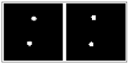
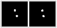
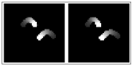
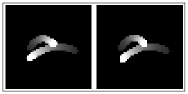
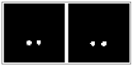
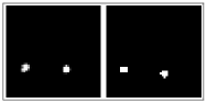
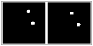
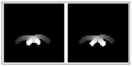
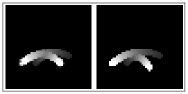
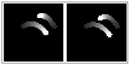
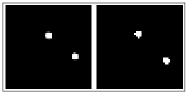
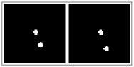
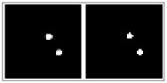
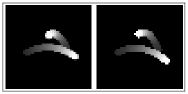
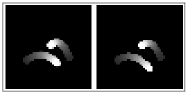
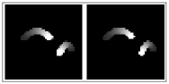
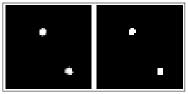
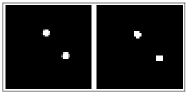
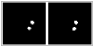
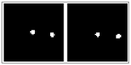
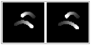
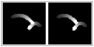
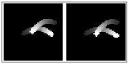
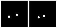
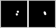
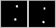
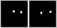
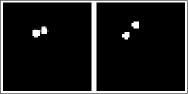
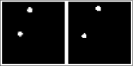
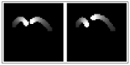
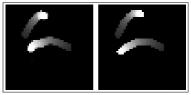
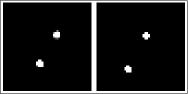
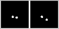
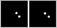
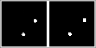
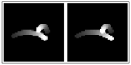
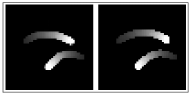
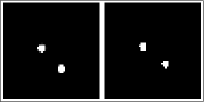
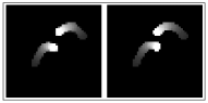
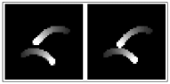
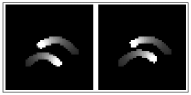
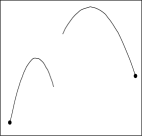
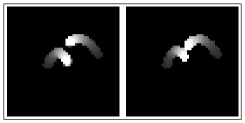
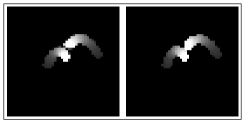
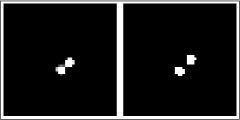
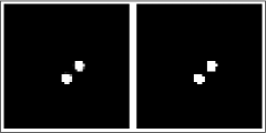
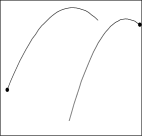
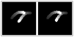
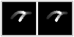
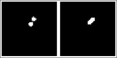
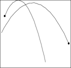
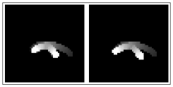
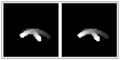
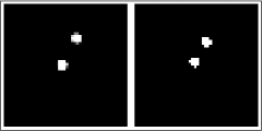
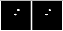
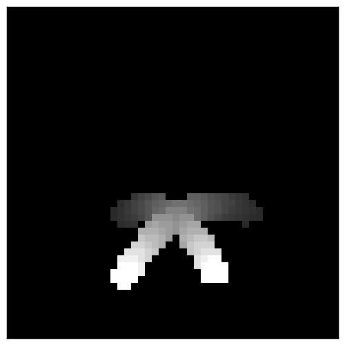
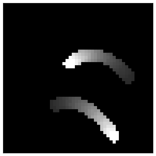
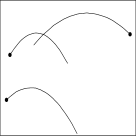
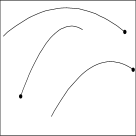
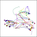
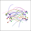
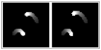
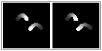
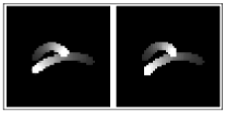
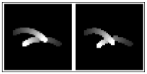
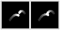
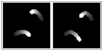
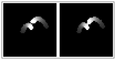
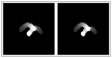
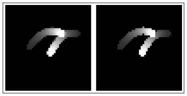
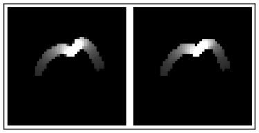
Two examples of sequences, each containing two cannonballs moving in opposite directions, are given in Fig. 1—the images are overlaid in time such that lighter shades correspond to more recent images.
The observed dynamics in the pixel space are high-dimensional and non-linear. However, the intrinsic dynamics can be described on the low-dimensional manifold of positions and velocities by simple dynamical systems. In the sections that follow, we show that the explicit representation of such latent dynamics enables us to infer positions using exact and efficient techniques. We also show that our approach enables us to answer different questions using the learned dynamics without the need to retrain or modify the model.
2.1 Generative model
We assume that the generative process underlying the observed images consists of two main parts: A part that describes the objects dynamics in the low-dimensional manifold of positions and velocities through a linear state-space model, and a part that renders the latent positions of the objects into the images through a highly non-linear process.
2.1.1 Rendering latent object positions into images
We use a set of auxiliary variables to explicitly represent the latent positions of object in the two-dimensional plane. Given the positions of all objects at time , , an image is generated by recurrently rendering each on . We start with , which represents a latent state vector from which an empty image canvas is generated, with denoting an unknown parameter vector. For , we iterate
| (latent attention mask) | |||||
| (object ’s state contribution) | |||||
| (1) |
and finally generate the image as
| (2) |
The symbol indicates element-wise vector multiplication, and . The ’s and ’s indicate weight matrices and biases, and are all included in the unknown parameters of the generative model.
This rendering process is illustrated in Fig. 2. The final state , which is transformed in Eq. (2) so that can be sampled, should contain information from all objects. To achieve that, the state is iteratively updated through Eq. (1) to incorporate the contribution from object , . This is obtained through an attention mask vector with elements in the interval , which specifies what information from object should be included and what information from should be retained.
2.1.2 Latent dynamics
We model the latent positions of each object, , using a hidden Markov model with linear Gaussian hidden-state and output, also known as linear Gaussian state-space model (LGSSM) barber11inferenceA ; chiappa06phd , i.e.
| (3) |
where denotes the density of a Gaussian random variable with mean and covariance . We use the constraints (where indicates horizontal and vertical matrix concatenation, denotes the identity matrix, and denotes the sampling period) and to obtain a description of Newtonian laws, such that the vector represents positions and velocities, and the force (which is assumed to be a constant over time). We include , , and in the generative model parameters .
Objects may start moving from disjoint sets of initial positions and velocities; for instance from the left, the right but not the center of . To allow the model to not put probability mass on initial positions and velocities that might never be helpful in explaining , the initial positions and velocities are drawn from a component Gaussian mixture, i.e.
| (4) |
We additionally include , and in the generative model parameters . The joint density of all random variables factorizes as
| (5) |
where and . The full generative model combines Eq. (2) with Eq. (5) to yield
The backbone of the model is illustrated in Fig. 2.
The advantage of this formulation for the latent dynamics is that quantities such as the smoothed distribution , the likelihood , or the most likely mixture component , can be computed exactly in operations, using message passing algorithms such as the Kalman filtering and Rauch-Tung-Striebel smoothing barber11inferenceA ; chiappa06phd .
2.2 Inference and Learning
The non-linearity of the rendering process makes the computation of , , and of quantities like needed for estimating the positions of object , intractable. We address this problem using a recent approach to variational methods known as variational auto-encoding (VAE) kingma14autoencoding ; rezende14stochastic .
The basic principle of variational methods is to introduce a tractable approximating distribution111Whilst in practice we need to consider all observed sequences in the KL, to simplify the notation we focus the exposition on one sequence only. to the intractable distribution via the Kullback-Leibler divergence
Given that
where we omitted super and subscript indices and used the notation to indicate averaging wrt , we obtain a lower bound on , i.e. with
If were tractable and we were able to perform marginalization on , we could find the optimal (parameters ) and by maximizing the bound; see chiappa08bayesian ; chiappa14explicit for traditional approaches to variational methods in the temporal setting. However, this is not the case for our generative model choice, and thus we instead use the more recent VAE approach to variational methods, where a Monte-Carlo approximation of the intractable is deployed.
The VAE approach consists in rewriting the bound in the form for a parameter free distribution , such that the gradient of with respect to is given by —this is often called reparemetrization trick. We can then approximate the gradient with the Monte-Carlo estimate
| (6) |
In our case, the formulation of the latent dynamics described above enables us to avoid employing a full approximation of , and instead to decompose this distribution as a product of the exact tractable distribution and an approximation of , i.e.
Thanks to this representation, the bound can be expressed as
This gives
| (7) |
We model using a recurrent neural network with states as in Fig. 2. More specifically we assume and use the reparametrization , under the assumption with . We describe this inference network in more details in the next section.
2.2.1 Inference network
As shown in Fig. 2, the inference network iterates a latent state vector over and . Starting with at time-step , we recurrently iterate
| (latent attention mask) | |||||
| (object ’s state contribution) | |||||
| (8) |
to compute a vector for each of the objects at time step . Similar to the generative model in Sec. 2.1.1, there is an attention mask that specifies how much of each component of we should keep. The mask is a function of the visible image , as well as the recurrently computed values for both the previous object at this time-step, and this object and the previous time-step. There is also a contribution coming from image for object . The combination of and is used to update . Samples from are generated as
| (9) |
where . In this computation, external Gaussian noise is inserted in a computation graph, and transformed—this ensures that the Monte-Carlo estimate in Eq. (6) is fully differentiable.
The ’s and ’s denote weight matrices and biases, and are included in the inference network parameters . The recurrent process at time-step depends on , and an initial state for each object is learned through parameters 222In practice, as the state encodes which way we can interrogate to infer , we have obtained better results by learning separate that depend on the number of objects in the image..
Note that appears in Eqs. (8) and (9) as input to every step at time-step . This is important: To infer the position , we need to consider the latent representation of object (actually 1 to ) in the previous image, as well as , which contains a rolled-up representation of objects 1 to in this image. Both these representations need to act on to infer .
2.2.2 Learning
In the Kullback-Leibler divergence term in Eq. (7), can be expressed in analytic form. Both the first term in Eq. (7) and in the KL divergence term can be stochastically estimated using a sample . For such a sample,
| (10) |
To compute Eq. (10), we take as “observations”, and for each mixture component we run a Kalman filter to obtain the log-likelihood . The objective function is the sum of the bounds in Eq. (7) over all sequences in the training dataset. The negative of this objective is minimized via a stochastic gradient descent algorithm, using mini-batches from the dataset.
2.3 Limitations
One of the main limitations of our approach is that, as does not explicitly incorporate the LGSSM dynamics, the objective function can have many sub-optimal local maxima. As common in the VAE literature, we address such a decoupling between the generative model and variational distribution by annealing the KL term in the bound to ensure that the dynamics are correctly accounted for during training. More advanced methods in the literature consist in incorporating the unknown latent dynamics into by essentially letting the dynamics be a “regularizer” to the parameters . “Structured inference networks” provide a framework for achieving this lin18variational . In pearce2018comparing we show that this approach leads to better inference and more stable results than annealing for the case of learning the dynamics of one object from pixels—it not obvious how this can be extended to the multiple-object scenario.
A more general limitation of our approach is its applicability to images that contain arbitrary backgrounds and objects, and nonlinear interactions between objects.
3 Results
In this section, we evaluate our approach on inferring latent positions, and on image generation and interpolation using artificially generated images describing the movement of cannonballs, see the examples shown in Fig. 1.
3.1 Dataset
We generated image sequences of length describing the movement of up to three cannonballs. Noisy positions were generated with an LGSSM formulation of Newtonian laws, as described in Sec. 2.1.2, with sampling period ; force , where is the gravitational constant; ; and .
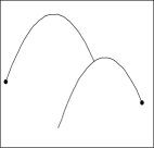
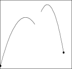
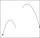
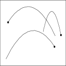
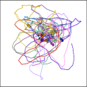
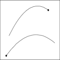
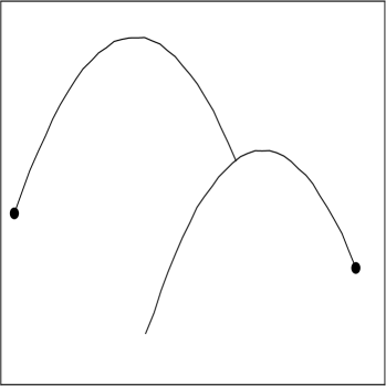
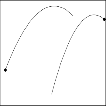
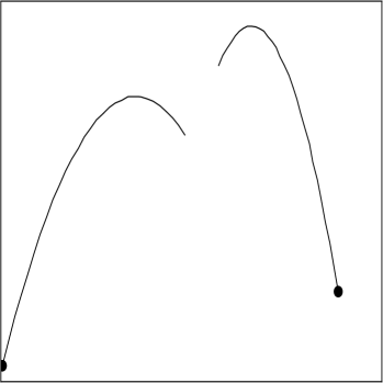
Each ball was shot with random shooting angle in the interval , from either the left side of the -axis in the interval or the right side of the -axis in the interval , where indicates the maximum possible displacement at when starting in . The initial position on the -axis was sampled in the interval . The initial velocity was sampled in the interval . The resulting velocity on the -axis, , was flipped in sign if the ball was shot from the right side of the image. Some examples of trajectories are shown in black in Fig. 3, with circles indicating initial positions.
To render the positions into white patches of radius in the image, the generated positions were re-scaled to lie in the interval , where indicate the height and width of the image. This re-scaling ensured that each ball was always fully contained in the image. We also experimented with similar datasets with and , obtaining similar results. With the problem is easier in terms of dimensionality, but the latent positions are less identifiable, as close positions in the latent space might induce the same position in the image.
3.2 Initialization and training
The dataset consists of sequences with balls. Importantly, as the networks in Fig. 2 can dynamically unroll, the model was trained on all such sequences jointly. We used to inform the networks of how many steps to unroll for each image sequence.
As the initial cannonballs are roughly separated into two main clusters, we assumed two mixture components, i.e. . Although a higher would induce a more refined grouping of initial positions and velocities, our experiments indicate that was sufficient to obtain accurate results.
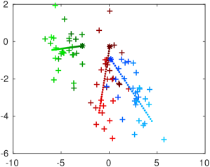
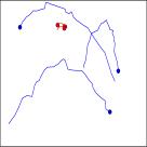
We experimented with different types of initialization for the LGSSM. Good results were obtained as long as smoothness in the dynamics was enforced so that we could guide the inference network toward smooth trajectories (as explained below). One example of such an initialization is to set and as above with , , , and ; sample the part of corresponding to positions from a standard Gaussian distribution and set the part corresponding to the velocities to zero; and set : This ensures symmetry breaking without imposing any meaningful prior on the clusters.
The absence of force gives rise to positions that form straights lines, as the dots in Fig. 4, which represent the first two dimensions of for . The high emission noise gives rise to highly non-smooth (crosses). This initialization induces very different dynamics from the ground-truth and does not assume any clustering, but encodes prior information that objects move smoothly in time.
For the rendering and inference networks in Secs. 2.1.1 and 2.2.1, the weight matrices entries were randomly initialized from , where is the number of matrix elements. All biases were initialized to zero. The dimension of the latent state was set to 1024. We used the Adam optimizer with learning rate 0.001, mini-batch size 20, and default values , , . Training was stopped after iterations.
To guide the inference network toward smooth trajectories we kept the LGSSM parameters fixed to their initial values for the first iterations, and only optimized for all other parameters. This initialization loosely gives temporal coherence between the inference network and the renderer, for different images. The model was then trained jointly, first by changing the objective function by multiplying the KL term in Eq. (7) with a weight , starting at , and annealing down to one. This avoids the LGSSM parameters from too quickly modelling the output of a (still very sub-optimal) , and stagnating at a local maximum. This process initializes the model, after which end-to-end training proceeds.
3.3 Inferring latent positions from image sequences
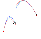
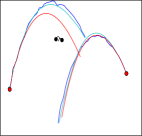
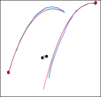
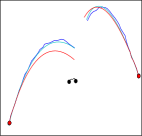
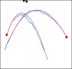
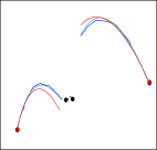
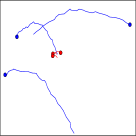
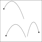
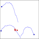
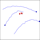
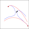
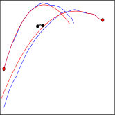
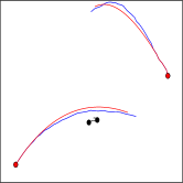
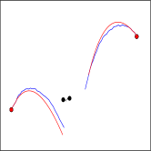
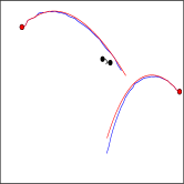
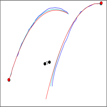
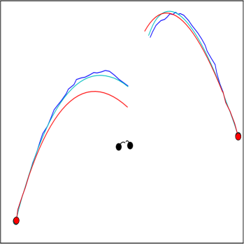
In Fig. 3 we show estimates of positions from the inference network. The ground-truth trajectories from which each image sequence is generated are shown in black. The inference network means are plotted in blue. Notice that each plot is scaled differently to aid qualitative evaluation. For that reason, we also selected a run with minimum rotation, but the latent positions can only be retrieved up to re-scaling and rotation. The larger scale of the inferred trajectories is highlighted by re-plotting the ground-truth trajectories (red lines) together with the inferred positions. These figures demonstrate that our model can accurately infer latent positions from the sequences of images in an unsupervised way.
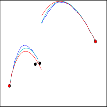
In Fig. 5(a), we show the inference network means for a batch of image sequences at three stages of training (for a case in which ), illustrating how the model learns over time. To highlight the challenge in learning to disentangle the objects dynamics, and the importance of initially strongly regularizing it to be close to the LGSSM during training, Fig. 5(b) shows an example in which we fail to learn an accurate inference network despite having learned accurate LGSSM dynamics. The ground-truth trajectories (black; left) and the trajectories generated from the learned LGSSM dynamics (red; right) are very similar. On the other hand, the inference network means (blue; right) swap the ball when reaching the middle part of the image: Rather than learning a successful attention mechanism, the inference network has learned to attend to the left part of the image for one ball and to the right part of the image for the other ball.
3.4 Multi-step ahead generation of images
To benchmark against a standard deep-learning model for multi-step ahead generation of images, we compared our model to an encoder-decoder long-short term memory model (ED-LSTM) hochreiter97long on the task of generating the 25 images following five observed images .
The structure of the ED-LSTM is represented in Fig. 7: At each time-step , the hidden state generates an image through a decoding transformation. For the first time-steps, receives an encoded version of the previous ground-truth image , as well as , as input. From time-step onward, receives an encoded version of the previous ground-truth image during training, or an encoded version of the previous generated image when the model is used in a multi-step ahead generation mode. We experimented with both convolutional and fully connected encoding and decoding transformations. The best results were obtained with one or two fully connected layers and dimension 2048 for . (All layers except the last were followed by a ReLU activation. The decoder last layer was followed by a sigmoid activation.) We used the same weights and biases initialization and optimizer settings as for our model.
To generate images with our model, we first inferred as the means of the inference network, for each object . Using the inferred , we computed the most likely mixture component as ] by running a Kalman filter. The filtered means of were then used as initial conditions to generate with the learned LGSSM dynamics (Eq. (3)). Finally images were generated through rendering of (Eqs. (1) and (2)).
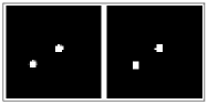
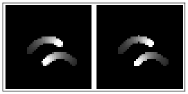
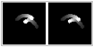
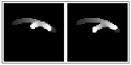
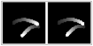
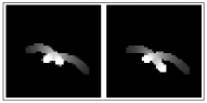
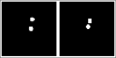
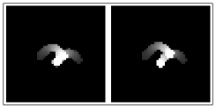
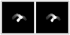
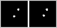
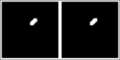
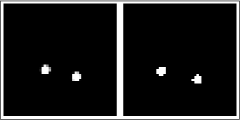
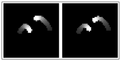
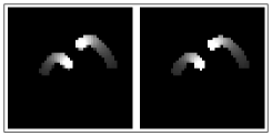
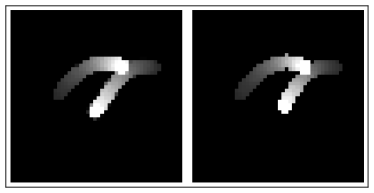
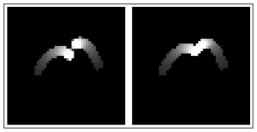
In Fig. 6, we show generated versus ground-truth images overlaid in time, for four sequences (more examples are given in the Appendix). For generation, our averaged test loss over the 25 time-steps was 0.691, using only eight as latent state dimension for the dynamics (). In contrast, the ED-LSTM’s test loss was 0.693, with 2048 as latent state dimension for the dynamics. Some examples of trajectories generated by our model are shown in Fig. 8.
Generated vs | Interpolated vs
3.5 Inference using past and future observations
Our model can interpolate missing images (and positions) from past and future images, a task that cannot be solved by the ED-LSTM without model adjustment and retraining.
We evaluated how our model performs in inferring the latent positions and images in the intermediate time-steps , based on observing the first and last five images and . The model should be able to use information from the future to produce more accurate latent positions than the ones that would be estimated by forward generation as in Fig. 8.
To solve the task, we first used to obtain and the most likely mixture component ; images at time-steps were then generated by the mechanism explained above. The inference network was run with the generated images to obtain a warmed-in state , which was then used as initial state for another run of the inference network with observed images to infer . We finally used and as observations in a Rauch-Tung-Striebel smoother to interpolate the missing trajectories , assuming that the observations at the intermediate time-steps were missing (integrated out from the model).
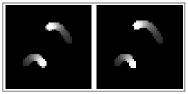
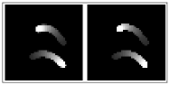
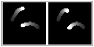
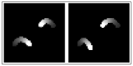
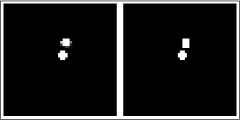
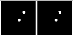
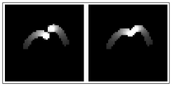
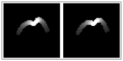
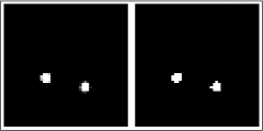
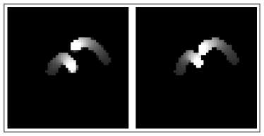
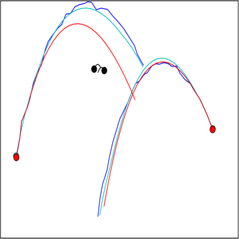
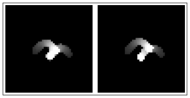
Some examples of obtained results are shown in Fig. 9 (more examples are given in the Appendix). We show the ground-truth trajectories in black, in blue, the generated trajectories in red, and the interpolated trajectories in cyan. The interpolation corrects the generated trajectories by bringing them closer to (obtained by observing the images at all time-steps) whilst maintaining the smoothness of dynamics constraints. To show the results of this correction mechanism in the pixel space, below the trajectories, from left to right, we show the generated versus ground-truth images and the interpolated versus ground-truth images, overlaid in time.
4 Conclusions
This paper describes an unsupervised approach to disentangle the dynamics of objects from pixels. We showed that it is possible for an inference network that is recurrent over both time and object number to sequentially parse each image to determine latent object positions. The model is regularized with a mixture of linear Gaussian state-space models, which encourages temporal coherence between latent positions extracted from images. Whilst the considered images of cannonballs are much simpler than those that would be encountered in most real-world applications, we nevertheless successfully demonstrated the usefulness of recovering interpretable latent structure in an unsupervised way and, more generally, of building structured generative models for high-dimensional visual stimuli.
References
- (1) M. Babaeizadeh, C. Finn, D. Erhan, R. Campbell, and S. Levine. Stochastic variational video prediction. In 6th International Conference on Learning Representations, pages 1–14, 2018.
- (2) Y. Bar-Shalom and X. R. Li. Estimation and Tracking: Principles, Techniques, and Software. Artech House, 1993.
- (3) D. Barber, A. T. Cemgil, and S. Chiappa. Inference and estimation in probabilistic time series models. Bayesian Time Series Models, pages 1–31, 2011.
- (4) S. Blackman and R. Popoli. Design and Analysis of Modern Tracking Systems. Artech House, 1999.
- (5) S. Chiappa. Analysis and Classification of EEG Signals using Probabilistic Models for Brain Computer Interfaces. PhD thesis, EPF Lausanne, Switzerland, 2006.
- (6) S. Chiappa. A Bayesian approach to switching linear Gaussian state-space models for unsupervised time-series segmentation. In Proceedings of the Seventh International Conference on Machine Learning and Applications, pages 3–9, 2008.
- (7) S. Chiappa. Explicit-duration Markov switching models. Foundations and Trends in Machine Learning, 7(6):803–886, 2014.
- (8) S. Chiappa, S. Racanière, D. Wierstra, and S. Mohamed. Recurrent environment simulators. In 5th International Conference on Learning Representations, 2017.
- (9) E. L. Denton and V. Birodkar. Unsupervised learning of disentangled representations from video. In Advances in Neural Information Processing Systems 30, pages 4414–4423, 2017.
- (10) C. Finn, I. J. Goodfellow, and S. Levine. Unsupervised learning for physical interaction through video prediction. In Advances in Neural Information Processing Systems 29, pages 64–72, 2016.
- (11) M. Fraccaro, S. Kamronn, U. Paquet, and O. Winther. A disentangled recognition and nonlinear dynamics model for unsupervised learning. In Advances in Neural Information Processing Systems 30, pages 3604–3613, 2017.
- (12) M. Fraccaro, S. K. Sønderby, U. Paquet, and O. Winther. Sequential neural models with stochastic layers. In Advances in Neural Information Processing Systems 29, pages 2199–2207, 2016.
- (13) Y. Gao, E. W. Archer, L. Paninski, and J. P. Cunningham. Linear dynamical neural population models through nonlinear embeddings. In Advances in Neural Information Processing Systems 29, pages 163–171, 2016.
- (14) S. Hochreiter and J. Schmidhuber. Long short-term memory. Neural Computation, 9(8):1735–1780, 1997.
- (15) M. Johnson, D. K. Duvenaud, A. Wiltschko, R. P. Adams, and S. R. Datta. Composing graphical models with neural networks for structured representations and fast inference. In Advances in Neural Information Processing Systems 29, pages 2946–2954, 2016.
- (16) D. P. Kingma and M. Welling. Auto-encoding variational Bayes. In 2nd International Conference on Learning Representations, 2014.
- (17) R. Krishnan, U. Shalit, and D. Sontag. Structured inference networks for nonlinear state space models. In Proceedings of the Thirty-First AAAI Conference on Artificial Intelligence, pages 2101–2109, 2017.
- (18) W. Lin, N. Hubacher, and M. E. Khan. Variational message passing with structured inference networks. In 6th International Conference on Learning Representations, 2018.
- (19) J. Oh, X. Guo, H. Lee, R. L. Lewis, and S. Singh. Action-conditional video prediction using deep networks in Atari games. In Advances in Neural Information Processing Systems 28, pages 2863–2871, 2015.
- (20) M. Pearce, S. Chiappa, and U. Paquet. Comparing interpretable inference models for videos of physical motion. In Symposium on Advances in Approximate Bayesian Inference, 2018.
- (21) D. J. Rezende, S. Mohamed, and D. Wierstra. Stochastic backpropagation and approximate inference in deep generative models. In Proceedings of the 31st International Conference on Machine Learning, pages 1278–1286, 2014.
- (22) N. Srivastava, E. Mansimov, and R. Salakhutdinov. Unsupervised learning of video representations using LSTMs. In Proceedings of the 32nd International Conference on Machine Learning, pages 843–852, 2015.
- (23) W. Sun, A. Venkatraman, B. Boots, and J. A. Bagnell. Learning to filter with predictive state inference machines. In Proceedings of the 32nd International Conference on Machine Learning, pages 1197–1205, 2016.
- (24) N. Watters, A. Tacchetti, T. Weber, R. Pascanu, P. Battaglia, and D. Zoran. Visual interaction networks. CoRR, abs/1706.01433, 2017.
Appendix. Multi-step ahead generation of images & inference using past and future observations