Continuity and discontinuity of kirigami’s high-extensibility transition: a statistical-physics viewpoint

Abstract

Recently, kirigami’s high extensibility has been understood as a transition in the force-elongation curve. In this paper, we consider a model, which modifies our previous model, to show a striking analogy between the present theory and Landau theory of continuous thermodynamic transitions, if we regard a rotation angle and elongation of kirigami as the order parameter and the inverse temperature, respectively. The present study opens a new avenue in physics, pointing out the importance of the distinction between discontinuity and continuity of the high-extensibility transition in an elementary kirigami structure, and showing that the mechanical response of kirigami can be understood using the tools of statistical physics, which have been proved to be useful in many fields of physics.

Origami and kirigami, Japanese traditional craft technique based on folding and/or cutting paper, have been received extensive attention in scientific fields because of their potential to impart sheet materials to mechanical and functional properties with simple patterning miura1985 ; xu2017origami . Resulting applications have been frequently regarded as mechanical metamaterials shan2015design ; bertoldiexploiting or tunable mechanical devices bertoldi2017flexible . The basic kirigami structure, formed by patterning parallel cuts on a sheet, makes sheet materials highly stretchable, which is shown even for graphene sheets GraphenKirigami2015Nature ; GraphenKirigami2014PRB . The high stretchability emerges from the transition from the in-plane to out-of-plane deformation, which is accompanied by a buckling-induced rotation of each unit of the structure isobe2016initial . While other cut patterns have been studied to explore versatile possibilities of the application of kirigami rafsanjani2017buckling ; hwang2018tunable , high stretchability of kirigami has been one of the important properties of kirigami. This property has been applied to varieties of materials such as conducting nanocomposites Kirigami2015NatMat , piezoelectric materials hu2018stretchable , metallic glass chen2018highly , and thermally responsive materials tang2017programmable , and to specific devices such as stretchable strain sensor sun2018kirigami and flexible film bioprobe morikawa2018ultrastretchable . Some researchers have focused on other available characteristics of kirigami structures. The buckling-induced rotation has been exploited for developing solar-tracking batteries KirigamiSolarNC2015 and dynamic shading systems yi2018developing . Frictional and interfacial properties have been utilized for fabricating soft actuator rafsanjani2018kirigami and enhancing film adhesion zhao2018kirigami , respectively. Although widely studied from application-oriented perspectives, the basic physical understanding of the high extensibility of kirigami is still premature, which is the focus of the present study.

.

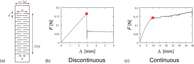
Figure 1: (a) Geometry of a simplified kirigami specimen. (b, c) Two typical examples of the force $F$ as a function of the elongation $\Delta$ in the vicinity of transition point, one exhibiting an abrupt (discontinuous) transition and the other exhibiting a (piece-wise) continuous transition. The former is obtained from a ridged polystyrene plate of Young’s modulus $E=3.1$ GPa ($h=0.2$ mm, $w=40$ mm, $d=2$ mm), while the latter from a soft elastomer sheet of $E=7.9$ MPa ($h=1$ mm, $w=30$ mm, $d=5$ mm).

As already mentioned above, the high stretchability of the basic kirigami structure (see Fig. 1(a)) has been explained by a simple model based on bending energy isobe2016initial . Experimentally, this transition manifests as a transition in the force-elongation curve. The transition could be an abrupt or a smooth transition and this difference seems to be dependent on materials used for fabricating specimens and the geometries of the cut patterns, as shown in the results reported from various groups chen2018highly ; sun2018kirigami ; hu2018stretchable (see Discussion): we provide typical experimental results for the two opposite cases in Fig. 1(b) and (c). An interesting issue here is whether this transition could be regarded as a thermodynamic transition and if this is the case whether the high-extensibility transition is continuous or discontinuous. In fact, in our recent work isobe2019discontinuity , we showed that our previous model proposed in isobe2016initial predicts a discontinuous transition and the prediction on the ratio between the forces just before and after the jump agree semi-quantitatively with experimental data obtained from kirigami samples made of Kent paper.

Here, we generalize our previous model and show that the kirigami’s high-extensibility transition can physically be identified with Landau theory of the second-order transition cardy1996scaling ; goldenfeld2018lectures , if we regard a rotation angle $\theta$ and elongation $\delta$ of each unit as the order parameter and the inverse temperature, respectively. We briefly discuss the possible mechanism of the kirigami’s transition becoming a discontinuous transition.

Geometry of a unit of kirigami under tension.— In this study, we consider a simplified kirigami structure, whose non-deformed geometry is specified in Fig. 1(a). An elementary unit of kirigami is defined as each of $2N$ strips, whose width, height, and thickness are respectively given by $w,d$, and $h$ with $w\gg d$ (see Fig. 1(a)). The ($2n-1$)-th elementary unit (from the top) is connected at the left and right edges of volume $hd^{2}$ with the $2n$-th elementary unit ($n=1,\cdots N$).

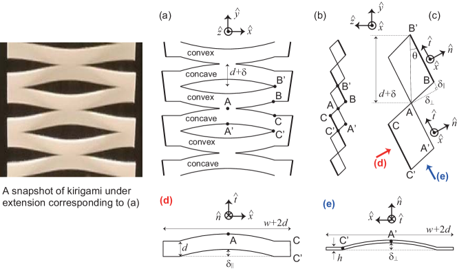
Figure 2: Kirigami’s geometry under a given elongation $\delta=\Delta/(2N)$. In the figure, the vectors, $\hat{x},\hat{y},\hat{t},$ and $\hat{n}$ are unit vectors, defined in the text, and used to show the plane on which the corresponding illustration is drawn. (a) Front view of an extended kirigami. (b) Side view. (c) Magnified side view. (d) The unit of kirigami containing the points A, A’, C, and C’ seen from the direction $\hat{n}$. (e) The same unit seen from the direction of $\hat{t}$.

In the previous study, we considered two modes of deformation. In the in-plane deformation, the central part of volume $hwd$ of the ($2n-1$)-th [$2n$-th] elementary unit bends ”downwards” [”upwards”] such that the arc of length $w$ and the center of this arc are on the original plane and the center is located below [above] the unit. In the out-of-plane deformation, the central part of volume $hwd$ of the ($2n-1$)-th [$2n$-th] elementary unit bends ”forwards” [”backwards”] such that the arc of length $w$ and the center of this arc are on the plane rotated from the original plane by a finite (small) angle and the center is located in front of [behind] the unit.

In the present study, we allow the simultaneous existence of these two modes. (We disallow it in the previous study.) Such a general deformation is described in Fig. 2, which is explained in detail below. The in-plane and out-of-plane deformation in the previous study correspond to the special cases in which $(\delta_{\perp},\theta)=(0,0)$ and in which $\delta_{\|}=0$, respectively.

In Fig. 2, the specimen is elongated by the amount $\Delta$ and, thus, each unit is elongated by $\delta=\Delta/(2N)$, as shown in Fig. 2(a) and the corresponding snapshot on the left side. Here, the unit vectors in the $x,y$ and $z$ directions are given by $\hat{x}$, $\hat{y}$, and $\hat{z}$, respectively. In Fig. 2(a), drawn on the $x-y$ plane, the surface of the central part of volume $hwd$ of the ($2n-1$)-th [$2n$-th] unit is ”concave” [”convex”] such that, for example, C and C’ are closer to you than A and A’ [A is closer to you than B]. The side view of Fig. 2 (a) is given in (b), which is drawn on the $y-z$ plane. A part of (b) is magnified in (c), in which the unit vectors $\hat{t}$ and $\hat{n}$ are respectively shown as the tangential and normal vectors on the surface of an above-mentioned element of kirigami, with the angle between the vector $\hat{t}$ and $\hat{y}$ being $\theta$. (Although each element is not on a plane but on a curved surface, $\hat{t}$ is identical at any point on the curved unit surface (and thus uniquely defined), and $\hat{n}$ can also be uniquely defined) In general, for each element ”rotated by the angle $\theta$” under the given elongation $\delta$, the deformation is characterized by the vector

$$\vec{\delta}_{T}=\delta_{\|}\hat{t}+\delta_{\perp}\hat{n}.$$ (1)

In Fig. 2(c), vectors $\overrightarrow{AB}$, $\overrightarrow{CA}$, and $\overrightarrow{C^{\prime}A^{\prime}}$ are, for example, identical to the vector $\vec{\delta}_{T}$. As clear from Fig. 2(c), $\delta_{\|}$ and $\delta_{\perp}$ satisfy the following relations:

$$(d+\delta)\cos\theta =d+\delta_{\|}$$ (2)

$$(d+\delta)\sin\theta =\delta_{\perp}$$ (3)

This means that as illustrated in (d) and (e), the deformation of each element can be regarded as a superposition of the bending in the $\hat{t}-x$ plane (the arc and its center characterizing the bending are on the $\hat{t}-x$ plane; see (d)) and the bending in the direction normal to this plane (the arc and its center are on $\hat{n}-x$ plane; see (e)), which will be called ”in-plane” and ”out-of-plane” deformations, respectively. Note that ”the plane” here does not refer to the original $x-y$ plane but the $\hat{t}-x$ plane.

Deformation energy of a unit of kirigami.— From the observations we have seen in Fig. 2(d) and (e), according to the standard formula for the bending energy, the energy for the specified deformation per unit element is given for $w\gg d,\delta$ by

$$U(\delta,\theta) =U_{\parallel}+U_{\perp}$$ (4)

$$U_{\parallel} =kE\frac{hd^{3}}{w^{3}}\delta_{\|}^{2}$$ (5)

$$U_{\perp} =kE\frac{h^{3}d}{w^{3}}\delta_{\perp}^{2}$$ (6)

where $E$ is Young’s modulus Landau ; isobe2016initial (see Sec. A of SM1 ). In fact, the numerical coefficient $k$ depends on the boundary conditions for bending and $k=(8/3)/(1-\nu^{2})$ with $\nu$ Poisson’s ratio Landau if we consider that the original straight line of length $w$ becomes a part of an arc assuming that $w\gg d,h$ as in the illustrations in Fig. 2. Other boundary conditions tend to increase the bending energies. (We have not considered ”net” stretching energy, which can be justified in the present case; see Sec. A of SM1 for the details.)

The independent variables for the above energy for a given set of $w$, $d$, and $h$ are in fact $\delta$ and $\theta$, as seen from Eqs. (2) and (3). By renormalizing the energy and lengths by using the energy unit $kEhd^{5}/w^{3}$ and the length unit $d$, we obtain a dimensionless expression:

$$\tilde{U}(\delta,\theta) =\tilde{U}_{\parallel}+\tilde{U}_{\perp}$$ (7)

$$\tilde{U}_{\parallel} =((1+\tilde{\delta})\cos\theta-1)^{2}$$ (8)

$$\tilde{U}_{\perp} =\tilde{h}^{2}((1+\tilde{\delta})\sin\theta)^{2}$$ (9)

with $\tilde{\delta}=\delta/d$ and $\tilde{h}=h/d$.

Transition behavior based on the energy.— The energy obtained above behaves as the Landau free energy for the second order transition, if we identify $\theta$ as the order parameter and $\delta$ as the inverse temperature. Figure 3 shows profiles of $\tilde{U}$ as a function of $\theta$ for various $\delta$ at $h/d=0.1$; at small $\delta$ the energy minimum appears at $\theta=0$ but as $\delta$ increases two minima appear symmetrically at $\theta=\pm$ $\theta^{\ast}$ with a finite $\theta^{\ast}$ ($>0$), which parallels Landau theory of critical phenomena. This feature is generic for the analytical structures as long as $h\ll d$ is satisfied, as discussed in Sec. B of SM1 , in which physical origins of the emergence of Landau’s scenario is elucidated. For the representation of the plots, we have introduced $\delta_{c}$ as

$$\tilde{\delta}_{c}=\delta_{c}/d=\tilde{h}^{2}/(1-\tilde{h}^{2})\simeq\tilde{h}^{2}$$ (10)

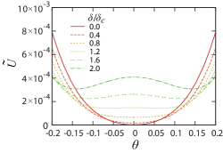
Figure 3: Free energy $\tilde{U}$ as a function of $\theta$ for various $\delta$ at $h/d=0.1$.

As seen in Fig. 3 (and shown precisely in Eq. (11) below), the quantity $\delta_{c}$ corresponds to ”the inverse critical temperature,” i.e., the value of $\delta$ at which the energy minima start to appear at nonzero values of the order parameter $\theta$. The corresponding scaling exponent is $1/2$, as shown in the following analytical expression derived in Sec. B of SM1 with the assumption $\theta\ll 1$ and thus exact near the critical point for the present model:

$$\theta^{\ast}=\left\{\begin{array}[c]{cc}0&\text{for }\delta<\delta_{c}\\ \left(2(1-\tilde{h}^{2})(\tilde{\delta}-\tilde{\delta}_{c})\right)^{1/2}&\text{for }\delta>\delta_{c}\end{array}\right.$$ (11)

Here, $\theta^{\ast}$ is theoretically predicted value of the rotation angle that is obtained as the minimum of $\tilde{U}(\tilde{\delta},\theta)$ in terms of $\theta$, by finding one of the solutions of the following equation for $\theta$:

$$\frac{\partial\tilde{U}(\tilde{\delta},\theta)}{\partial\theta}=0.$$ (12)

The order parameter in the present theory predicts a continuous transition, as seen in Eq. (11), whereas the order parameter in the previous theory isobe2016initial ; isobe2019discontinuity predicts a discontinuous transition. As summarized in Sec. C of SM1 , the quantity $\theta^{\ast}$ obtained in the previous theory jumps at $\delta=2\delta_{c}$ from $\theta=0$ to $\theta=\theta_{c}^{\ast}$ where $\theta_{c}^{\ast}$ is $\theta^{\ast}$ at $\delta=2\delta_{c}$, i.e., $\theta_{c}^{\ast}=\tan^{-1}\left(4\tilde{\delta}_{c}\right)^{1/2}\simeq 2\tilde{h}$ (see Eq. (33)). In other words, the expressions for $\theta^{\ast}$ in the present and previous models give the critical elongations, $\delta=\delta_{c}$ and $\delta=2\delta_{c}$, respectively, and thus the two models are similar in that the predicted critical elongations are the same at the level of scaling laws but are different because of an extra factor 2.

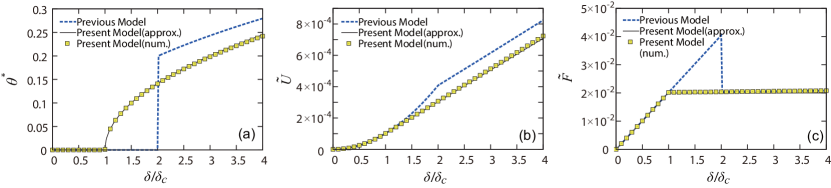
Figure 4: (a) The value $\theta^{\ast}$ of ”the order parameter” $\theta$ predicted by the theories as a function of ”the inverse temperature” $\delta$ for $h/d=0.1$, demonstrating that the present and previous models are continuous and discontinuous, respectively. (b) Normalized free energy minimized with respect to $\theta$ as a function of $\delta$ and (c) Normalized force - elongation curve for $h/d=0.1$.

The expression for $\theta^{\ast}$ in Eq. (11) is plotted in Fig. 4(a) under the label ”Present Model (approx.), which confirms a continuous transition. The plot labeled as ”Present Model (num.)” in Fig. 4(a) is obtained numerically finding the root of the condition in Eq. (12) without using the approximation $\theta\ll 1$. The numerical and approximate plots agree well with each other, which shows that the analytical expression is a good approximation in the range of $\delta$.

The plot labeled as ”Previous Model” in Fig. 4(a) is based on the analytical expression obtained in the previous model (see Sec. C of SM1 ). By comparing the three plots in Fig. 4(a), we can re-confirm the similarities and differences in the $\delta$-dependence of $\theta^{\ast}$ in the two models discussed above on the basis of the analytical expression.

The analytical expressions for $\tilde{U}(\tilde{\delta},\theta^{\ast})$, which is $\tilde{U}(\tilde{\delta},\theta)$ evaluated at $\theta=\theta^{\ast}$, and the force defined by $\tilde{F}=\left|-\partial\tilde{U}(\tilde{\delta},\theta^{\ast})/\partial\tilde{\delta}\right|$ (the force $F$ is normalized here by the unit $kEhd^{4}/w^{3}$) obtained in the present model are summarized in Sec. B of SM1 , and predict the following features of the present model: (1) $\tilde{U}(\tilde{\delta},\theta^{\ast})$ scales with $\tilde{\delta}^{2}$ and $\tilde{\delta}$ for $\delta<\delta_{c}$ and $\delta>\delta_{c}$, respectively, and the two branches are matched at $\delta=\delta_{c}$. (2) $\tilde{F}(\tilde{\delta})$ scales with $\tilde{\delta}$ and $\tilde{\delta}^{0}$ for $\delta<\delta_{c}$ and $\delta>\delta_{c}$, respectively, and the two branches are matched at $\delta=\delta_{c}$ (because $\tilde{\delta}\simeq\tilde{h}^{2}$ at $\delta=\delta_{c}$ for $\tilde{h}\ll 1$).

There are similarities and differences between the analytical expressions for $\tilde{U}$ and $\tilde{F}$ in the present model (see Sec. B of SM1 ) and those in previous model (see Sec. C SM1 ). (1) In both models, the quadratic $\tilde{\delta}$-dependence of $\tilde{U}(\tilde{\delta})$ is switched to the linear $\tilde{\delta}$-dependence at the transition point. (2) The spring constant (slope of the force-elongation curve) before the transition is exactly the same in the two theories. However, there are important qualitative differences in the two theories. (1) In the previous theory $\tilde{U}(\tilde{\delta})$ is piecewise continuous (discontinuous at the transition $\delta=2\delta_{c}$), whereas it is continuous at the transition $\delta=\delta_{c}$ in the present theory. (2) Accordingly, the force-elongation curve shows a discontinuous jump at the transition point in the previous theory, whereas it is (piecewise) continuous in the present theory; $\tilde{F}(\tilde{\delta})$ in Eq. (35) shows a drop from $\tilde{F}(\tilde{\delta})=4\tilde{\delta}_{c}$ to $2\tilde{\delta}_{c}$ at $\delta=2\delta_{c}$, while $\tilde{F}(\tilde{\delta})$ in Eq. (32) shows a jump-less crossover ($\tilde{F}(\tilde{\delta})=2\tilde{\delta}_{c}$ at $\delta=\delta_{c}\pm\varepsilon$ with $\varepsilon$ a small number).

The analytical expressions for $\tilde{U}$ and $\tilde{F}$ in the present model are plotted in Fig. 4(b) and (c) under the label ”Present Model (approx.),” from which we can re-confirmed the above features. The plots labeled ”Present Model (num.)” in Fig. 4(b) and (c) are, respectively, given by numerically evaluating Eq. (7) at $\theta=\theta^{\ast}$ (here, the value numerically obtained, by solving Eq. (12)) and by differentiating the plot in (b) with respect to $\delta$, on the basis of the definition of $\tilde{F}$ given above. We see that the plots labeled ”Present Model (approx.)” and ”Present Model (num.)” in (b) agree with each other, as in (c), which justifies again our approximate analytical expressions.

The plots for the previous model, labeled as ”Previous Model,” Fig. 4(b) and (c) are based on analytical expressions summarized in Sec. C of SM1 . By comparing the three plots in (b), as well as in (c), we can re-confirm the above-discussed similarities and differences. Note that Fig. 4(c) corresponds to the experimental results shown in Fig. 1(b) and (c).

Discussion.— The previous isobe2016initial and present theories predict the same scaling laws for the spring constant in the first regime, the critical elongation, and the force at large elongation. Thus, the agreement of these predictions with our experimental data shown in isobe2016initial ; isobe2019discontinuity justifies the present theory, as well as the previous theory.

One of the important issues demonstrated in this paper is the continuity and discontinuity in the high-extensiblity transition of kirigami for the present simple slit geometry. As shown above, this distinction is captured clearly in the framework of statistical physics if we focus on the appropriate order parameter, the rotation angle, and identify the elongation with the inverse temperature.

According to several previous studies, the transition in force-elongation curve seems to be discontinuous (e.g., hu2018stretchable ) or continuous (e.g., chen2018highly ; sun2018kirigami ) depending on conditions, although there has not been any systematic experimental investigation on the topic, except for a very recent article (but mainly in a more complex arrangement of silts) rafsanjani2019propagation . As demonstrated in Fig. 1(b) and (c), it has been suggested that when kirigami is made of paper or ridged plastic sheets transitions tend to be discontinuous (corresponding to our previous model, in which the simultaneous existence of ”purely in-plane and out-of-plane deformations” is disallowed), and when kirigami is made of soft gels transitions tend to be continuous (corresponding to our present model, in which the simultaneous existence is allowed). We note here that, by developing the technique of elastic charges, the force-elongation curve has recently been discussed in moshe2019nonlinear , and the importance of stress relief is discussed in moshe2019kirigami focusing only on the continuous case for a rather different non-slit geometry.

To deepen our understanding of the distinction between the continuity and discontinuity, we have to explore the effects ignored in our theories, such as friction and plastic deformation, and perform experiments focusing on these aspects with systematically changing parameters, such as thickness and elastic modulus. These topics will be discussed elsewhere.

In the emerging field of mechanics of metamaterials, the connection with critical phenomena in statistical physics has been lacking, although the scaling law (the usefulness of which is for physicists deeply rooted in the lessons learned from critical phenomena) and thermodynamic concepts have been explored in a number of recent publications yang2018multistable ; rafsanjani2019propagation and connections to bifurcation and nonlinear physics have been stressed in the literature, probably from historical reasons pippard1985response ; audoly2010elasticity ; cedolin2010stability . The key words such as the critical exponent and the order parameter, which are indispensable to describe critical phenomena, have been absent in the literature (except for a few bobnar2011euler ), although the classic Euler buckling can be discussed in the framework of Landau theory of critical phenomena, as explicitly demonstrated in see Sec. D of SM1 . (A scaling relation similar to Eq. (11) is shown for kirigami actuators dias2017kirigami , which is again not connected to critical phenomena.) Although the present kirigami’s transition is not a critical phenomenon, the remarkable analogy to Landau theory of critical phenomena demonstrated in the present study points out to the researchers in the field the potential of the powerful tools of statistical physics, which have been proved to be useful in many fields of physics including nonequilibrium statistical physics livi2017nonequilibrium .

Supplemental Material

.1 Bending energy of a plate and the effect of stretching

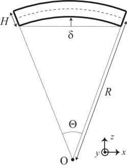
Figure 5: Bending of a plate of thickness $H$, length $L$, and width $W$ (in the $y$ direction).

We consider that a plate of thickness $H$ (in the $z$ direction in the undeformed plane state), length $L$ (in the $x$ direction in the plane state), and width $W$ (in the $y$ direction) bends such that the sides of length $L$ of the plate become an arc of radius $R$ where the arc and its center O are located on the $x-z$ plane (see Fig. 5). If we consider $r-\theta$ coordinate around this center on the $x-z$ plane, the plate occupies the region defined by the conditions $-H/2+R<r<R+H/2$ and $-\Theta/2<\theta<\Theta/2$. When ”net stretch” is absent, the area of the ”middle surface” located at $r=R$ (represented by the dashed line in Fig. 5) remains the original value $LW$. When ”net stretch” comes into play, this area becomes $L(1+\varepsilon_{0})W$ with $\varepsilon_{0}$ describing the size of stretch in the $\theta$ direction, whereas

$$R\Theta=L(1+\varepsilon_{0})$$ (13)

The stretch associated with the surface located as $r=R+\eta$ is given by $L(\eta)=(R+\eta)\Theta$ and the strain in the $\theta$ direction can be estimated as $\varepsilon(\eta)=(L(\eta)-L)/L$, which gives

$$\varepsilon(\eta)=\varepsilon_{0}+\eta(1+\varepsilon_{0})/R\simeq\varepsilon_{0}+\eta/R$$ (14)

when $\varepsilon_{0}\ll 1$. The bending energy thus scales as

$$U\simeq\int_{-H/2}^{H/2}d\eta E\varepsilon(\eta)^{2}WL(\eta)/2,$$ (15)

in which $\varepsilon(\eta)^{2}L(\eta)\simeq(\eta/R+\varepsilon_{0})^{2}L$ for $\varepsilon_{0}\ll 1$ and $\eta\ll R$. (The proportional coefficient is in general dependent on Poison’s ratio and boundary condition. Here, we focus on relation at the level of scaling laws and ignore the coefficient.) As a result, we obtain

$$U\simeq\frac{EWLR}{6}\left[\left(\varepsilon_{0}+\frac{H}{2R}\right)^{3}-\left(\varepsilon_{0}-\frac{H}{2R}\right)^{3}\right]$$ (16)

which gives

$$U\simeq\frac{EWLR}{3}\left[\left(\frac{H}{2R}\right)^{3}+3\frac{H}{2R}\varepsilon_{0}^{2}\right]$$ (17)

Introducing $\delta$ as the size of bending in the $z$ direction (see Fig. 5) and considering the geometrical relations, $R^{2}=(R-\delta)^{2}+(L(1+\varepsilon_{0})\cos(\Theta/2)/2)^{2}$ and $\delta=(L/2)\tan(\Theta/2)$ with Eq. (13), we obtain

$$2\delta R =L^{2}/4$$ (18)

$$\Theta =4\delta/L$$ (19)

for $\varepsilon_{0}\ll 1$ and $L\ll R$.

Equation (18) reduces the first term in Eq. (17) to the standard form $\simeq(8/3)EWLH^{3}(\delta/L^{2})^{2}$, from which we can derive Eqs. (5) and (6), at the level of scaling laws: the in-plane and out-of-plane deformations corresponding to $(W,L,H,\delta)=(h,w,d,\delta_{\parallel})$ and $(W,L,H,\delta)=(d,w,h,\delta_{\perp})$, respectively. The correction term in Eq. (17) proportional to $\varepsilon_{0}^{2}$ always produces a positive term, which means any ”net stretch” associated with bending is energetically unfavorable.

Stretching can nevertheless occur in some cases, depending on the boundary condition Landau . For example, when one tries to bend a circular plate, if the length of the circular edge is fixed the deformation is accompanied with stretch of the diameter (here, we consider a circle on a spherical surface); on the other hand, if the length of the diameter is fixed, the length of the circular edge should be shrunk.

In the present example, we can set the following boundary constraint (the length between the both ends of the plate fixed to $L$):

$$L=L(1+\varepsilon_{0})\cos(\Theta/2)$$ (20)

For $\varepsilon_{0}\ll 1$ and $L\ll R$, this boundary condition results in

$$\varepsilon_{0}=(\Theta/2)^{2}/2=2(\delta/L)^{2}$$ (21)

Under this edge boundary constraint set by Eq. (20), the full energy given in Eq. (17) can be expressed as

$$U\simeq EWL\left[(8/3)H^{3}(\delta/L^{2})^{2}+2H(\delta/L)^{4}\right]$$ (22)

The bending and stretch energies scale as $EWLH^{3}(\delta/L^{2})^{2}$ and $EWLH(\delta/L)^{4}$, respectively, and the ratio is $H^{2}:\delta^{2}$. The same scaling laws are given in Landau in a more general context.

However, the bending deformation of a unit element of the present kirigami shown in Fig. 1(a) occurs under no length constraint in the direction of $w$ (corresponding to the direction of $L$ in the present example). In the case of our kirigami in Fig.1(a), the ($2n-1$)-th [2$n$-th] unit element is constraint at the middle section (of length $d$) of the top [bottom] side of length $w+2d$, where the unit is connected to ($2n-2$)-th [($2n-1$)-th] unit. However, the left and right edge sections (of length $d$) of the bottom [top] side (of length $w+2d$) of the ($2n-1$)-th [$2n$-th] unit, where the unit is connected to the 2$n$-th [(2$n-1$)-th] unit, are not constrained and can freely move in the direction of $w$. [As a result, to minimize the energy, the distance between both edges of the unit element tend to become closer (because the edges are not constrained) as the kirigami sample is stretched at the top and bottoms ends.] Thus, stretching is not expected play any dominant roles in the present kirigami.

.2 Analytical details of the present model

We consider the expansion of $\tilde{U}(\tilde{\delta},\theta)$ in terms of $\theta$

$$\tilde{U}(\tilde{\delta},\theta)=\tilde{U}(\tilde{\delta},0)+A\theta^{2}+b\theta^{4}+c\theta^{6}+\cdots$$ (23)

and examine the behavior of $\tilde{U}(\tilde{\delta},\theta)$ for small $\theta$. For this purpose, we obtain the following expansion for the two energies in Eq. (7):

$$\tilde{U}_{\parallel} =\tilde{\delta}^{2}-\tilde{\delta}(1+\tilde{\delta})\theta^{2}+(\tilde{\delta}+3(1+\tilde{\delta}))(1+\tilde{\delta})\theta^{4}/12+\cdots$$ (24)

$$\tilde{U}_{\perp} =\tilde{h}^{2}(1+\tilde{\delta})^{2}(\theta^{2}-\theta^{4}/3+\cdots)$$ (25)

This implies

$$A =(1+\tilde{\delta})(-\tilde{\delta}+(1+\tilde{\delta})\tilde{h}^{2})$$ (26)

$$b =(1+\tilde{\delta})((3+4\tilde{\delta})-4(1+\tilde{\delta})\tilde{h}^{2})/12,$$ (27)

which can be re-expressed as in the following form (note that the following quantities can be obtained by the relation $A=[\partial^{2}\tilde{U}(\tilde{\delta},\theta)/\partial\theta^{2}]_{\theta=0}/2$ and $b=[\partial^{4}\tilde{U}(\tilde{\delta},\theta)/\partial\theta^{4}]_{\theta=0}/4!$):

$$A =-(1-\tilde{h}^{2})(\tilde{\delta}+1)(\tilde{\delta}-\tilde{\delta}_{c})$$ (28)

$$b =(1/3)(1-\tilde{h}^{2})(\tilde{\delta}+1)(\tilde{\delta}+\tilde{\delta}_{4})$$ (29)

with $\tilde{\delta}_{c}$ given by $\tilde{h}^{2}/(1-\tilde{h}^{2})$ as in Eq. (10) and with $\tilde{\delta}_{4}$ given by

$$4\tilde{\delta}_{4}=(3-4\tilde{h}^{2})/(1-\tilde{h}^{2}),$$ (30)

which suggest that, for $\tilde{h}<1$ and $\tilde{\delta}>0$ as in the present case, the coefficient $b$ is positive and the coefficient $A$ changes the sign at $\tilde{\delta}=\tilde{\delta}_{c}$. In such a case, for small $\theta$, Landau’s continuous transition is expected: a continuous transition occurs at $\tilde{\delta}=\tilde{\delta}_{c}\,$, i.e., when $A=0$. This is because, for the values $\tilde{\delta}$ at which $A$ is positive, $\tilde{U}(\tilde{\delta},\theta)$ as a function of $\theta$ has a single minimum at $\theta=0$ (note that $b$ is positive), but for the values $\tilde{\delta}$ at which $A$ is negative, $\tilde{U}(\tilde{\delta},\theta)$ as a function of $\theta$ has double minima at $\theta=\pm\theta^{\ast}$. The value of $\theta^{\ast}$ is obtained by solving the equation $\partial\tilde{U}(\tilde{\delta},\theta)/\partial\theta=0$ in terms of $\theta$. From this equation, we obtain $\theta^{\ast}=0$ and, for $\tilde{\delta}>\tilde{\delta}_{c}$, another solution $(\theta^{\ast})^{2}=-A/(2b)=(3/2)(\tilde{\delta}-\tilde{\delta}_{c})/(\tilde{\delta}+\tilde{\delta}_{4})$, which behaves as $2(1-\tilde{h}^{2})(\tilde{\delta}-\tilde{\delta}_{c})$ in the vicinity of $\tilde{\delta}=\tilde{\delta}_{c}$. In this way, we can derive Eq. (11) and we can justify analytically that the point $\delta=\delta_{c}$ is truly the transition point. From Eqs. (23), (7) and (11), for $\tilde{\delta}$, $\theta^{\ast}$, $\tilde{h}\ll 1$, we obtain

$$\tilde{U}(\tilde{\delta},\theta^{\ast}) =\left\{\begin{array}[c]{cc}\tilde{\delta}^{2}=\tilde{\delta}_{c}^{2}(\delta/\delta_{c})^{2}&\text{for }\delta<\delta_{c}\\ \tilde{\delta}_{c}^{2}+2\tilde{h}^{2}(\tilde{\delta}-\tilde{\delta}_{c})&\text{for }\delta>\delta_{c}\end{array}\right.,$$ (33)

$$\tilde{F}(\tilde{\delta}) =\frac{\partial\tilde{U}(\tilde{\delta},\theta^{\ast})}{\partial\tilde{\delta}}=\left\{\begin{array}[c]{cc}2\tilde{\delta}&\text{for }\delta<\delta_{c}\\ 2\tilde{h}^{2}=2\tilde{\delta}_{c}&\text{for }\delta>\delta_{c}\end{array}\right..$$ (36)

In Fig. 4(a), (b), and (c), the plots labeled as ”Present Model (approx.)” are based on Eqs. (11), (33), and (36), respectively.

.3 Analytical details of the previous model

In our previous work, we simply considered two possible modes of deformations and forbid the mixture of the two modes: (1) ”purely in-plane deformation,” in which $(\delta_{\perp},\theta)=(0,0)$, i.e., $\vec{\delta}=\delta_{\|}\hat{y}$ together with $\delta=\delta_{\|}$, and (2) ”purely out-of plane deformation,” in which $\delta_{\|}=0$ with a finite angle $\theta=\theta^{\ast}$, i.e., $\vec{\delta}=\delta_{\perp}\hat{n}$ together with $\tan\theta^{\ast}=\delta_{\perp}/d$ and $(d+\delta)^{2}=d^{2}+\delta_{\perp}^{2}$, which lead to

$$\theta^{\ast}=\left\{\begin{array}[c]{cc}0&\text{for }\delta<2\delta_{c}\\ \arctan\left((1+\tilde{\delta})^{2}-1\right)^{1/2}&\text{for }\delta>2\delta_{c}\end{array}\right.$$ (37)

The energy for the former deformation scales with $\delta^{2}$ (because of Eq. (4) with $\delta_{\perp}=0$ and $\delta_{\|}=\delta$) and that for the latter scales with $\delta$ (because of Eq. (4) with $\delta_{\|}=0$, together with $\delta_{\perp}^{2}=2d\delta$ in the limit $\delta\ll d$). This means that at lower energies the purely in-plane deformation has the lower energy but at higher energies the purely out-of-plane deformation becomes the lower. The transition point for $\delta$ is determined by matching the two energies, which is revealed to occur at $\delta=2\delta_{c}$. In summary, the previous theory results in the following expressions in the limit $\tilde{h}\ll 1$:

$$\tilde{U}(\tilde{\delta}) =\left\{\begin{array}[c]{cc}\tilde{\delta}^{2}&\text{for }\delta<2\delta_{c}\\ 2\tilde{h}^{2}\tilde{\delta}=2\tilde{\delta}_{c}\tilde{\delta}&\text{for }\delta>2\delta_{c}\end{array}\right.$$ (40)

$$\tilde{F}(\tilde{\delta}) =\left\{\begin{array}[c]{cc}2\tilde{\delta}&\text{for }\delta<2\delta_{c}\\ 2\tilde{h}^{2}=2\tilde{\delta}_{c}&\text{for }\delta>2\delta_{c}\end{array}\right.,$$ (43)

In Fig. 4(a), (b), and (c), the plots labeled as ”Previous Model” are based on Eqs. (37), (40), and (43), respectively.

.4 Buckling of thin plates and Landau theory of critical phenomena

We showed in the main text that kirigami’s transition can be viewed as the critical phenomenon described by Landau theory. A similar scenario emerges for the classic problem of buckling of thin plates (or beams) as explained in the following.

We again consider the situation in Fig. 5. However, this time we assume that the distance between the left and right ends becomes $L-\Delta$ from the original value $L$ with $\Delta>0$. In the case of pure bending, the area of the ”middle surface” located at $r=R$ (represented by the dashed line in Fig. 5) remains the original value $LW$. In general, this area becomes $L(1+\varepsilon_{0})W$ with $\varepsilon_{0}(<0)$ describing the size of shrinkage of the length of the neutral line in the $\theta$ direction to obtain Eq. (17) as before.

Introducing $\delta$ as the size of bending in the $z$ direction (see Fig. 5) as before and considering the geometrical relations, $R^{2}=(R-\delta)^{2}+(L(1+\varepsilon_{0})\cos(\Theta/2)/2)^{2}$ and $\delta=((L-\Delta)/2)\tan(\Theta/2)$ with Eq. (13), we again obtain Eqs. (18) and (19) for $\left|\varepsilon_{0}\right|\ll 1$ and $\Delta\ll L\ll R$.

In the present example, we have set the following boundary constraint (the length between the both ends of the plate fixed to $L-\Delta$):

$$L-\Delta=L(1+\varepsilon_{0})\cos(\Theta/2)$$ (44)

From this, we decompose $\Delta$ in the two components:

$$\Delta=\Delta_{B}+\Delta_{C}$$ (45)

with introducing the pure bending part and pure compression part defined, respectively, as

$$\Delta_{B} =L(\Theta/2)^{2}/2=2\delta^{2}/L$$ (46)

$$\Delta_{C} =\left|\varepsilon_{0}\right|L$$ (47)

Under the edge boundary constraint set by Eq. (44), the full energy given in Eq. (17) can be expressed as

$$U\simeq\frac{4EWH^{3}}{3L^{2}}\Delta_{B}+\frac{EWH}{2L}\Delta_{C}^{2}$$ (48)

The first term corresponds to the pure bending deformation scaling as $EH^{3}(\delta/L^{2})^{2}WL$. The second term to the pure compression, in which the plate remains flat and is subject to a homogeneous strain of $\varepsilon=\Delta/L$: the energy for pure compression scales as $E\varepsilon^{2}HWL=EWH\Delta^{2}/L$, which coincides with the second term at the level of scaling laws.

If we disallow the simultaneous existence of bending and compression, and compare the two energies, $(4/3)EWH^{3}\Delta/L^{2}$ and $(1/2)EWH\Delta^{2}/L$, which, respectively scale as $\Delta$ and $\Delta^{2}$, the pure compression energy $\sim\Delta^{2}$ is lower than the pure bending energy $\sim\Delta$ for small $\Delta$: the pure compression without bending is expected for small $\Delta$. However, the relative importance of the two energies is interchanged at the matching point: $\Delta=2\Delta_{c}$ with

$$\Delta_{c}=(4/3)H^{2}/L.$$ (49)

For large $\Delta$ ($\Delta>2\Delta_{c}$), the pure bending energy is lower than the pure compression energy and, thus, the pure bending is predicted for large $\Delta$. At the critical strain $\varepsilon=2\varepsilon_{c}$ with $\varepsilon_{c}=\Delta_{c}/L=(4/3)(H/L)^{2}$, the force acting on the both edges is derived by differentiating the bending energy with respect to $\Delta$ to obtain a result for the critical force divided by the width $W$: $P_{c}=F_{c}/W=(4/3)EH^{3}/L^{2}$. This corresponds to Euler buckling load $\pi^{2}EI/L^{2}$, where $I\simeq H^{3}$ in the present case. If we derive the force from the compression energy evaluated at the transition point $\Delta=2\Delta_{c}$, we obtain instead $(8/3)EH^{3}/L^{2}$, i.e., twice the value obtained from the bending energy. This difference between the forces at the transition point corresponds to the force jump in the kirigami model.

If we allow the simultaneous existence of bending and compression (this corresponds to the usual treatment in the field), we have to consider the full energy given in Eq. (22). For convenience, we change the set of unknown variables from $(\Delta_{B}$, $\Delta_{C})$ to $(\Delta$, $\delta)$ to have the following expression with the aid of Eqs. (45) to (47):

$$U\simeq\frac{8EWH^{3}}{3L^{3}}\delta^{2}+\frac{2EWH}{L^{3}}\left(\delta^{2}-L\Delta/2\right)^{2}$$ (50)

We renormalize the energy and length scales, respectively, by the energy and length scales $2EW^{5}H/L^{3}$ and $W$:

$$\tilde{U}\simeq-\tilde{L}(\tilde{\Delta}-\tilde{\Delta}_{c})\tilde{\delta}^{2}+\tilde{\delta}^{4}+\left(\tilde{L}\tilde{\Delta}/2\right)^{2}$$ (51)

with $\tilde{\Delta}_{c}$ defined in Eq. (49).

The last form is a typical Landau free energy, if we identify $\tilde{\delta}$ as the order parameter and $\tilde{\Delta}$ as the inverse temperature. When the compression is small ($\tilde{\Delta}<\tilde{\Delta}_{c}$), the coefficient of $\tilde{\delta}^{2}$ is positive: $\tilde{U}$ has a single minimum at $\tilde{\delta}=0$, which corresponds to the pure compression without bending. When the compression is large ($\tilde{\Delta}>\tilde{\Delta}_{c}$), the coefficient becomes negative and thus $\tilde{U}$ as a function of $\tilde{\delta}$ is convex near $\tilde{\delta}=0$; however, because of the coefficient of $\tilde{\delta}^{4}$ is positive, we have double minima at $\tilde{\delta}=\pm\tilde{\delta}^{\ast}$. This $\tilde{\delta}^{\ast}$ is the theoretically predicted value of $\tilde{\delta}$ for $\tilde{\Delta}>\tilde{\Delta}_{c}$ and is determined as one of the solutions of $\partial\tilde{U}/\partial\tilde{\delta}=0$, i.e., $-2\tilde{L}(\tilde{\Delta}-\tilde{\Delta}_{c})\tilde{\delta}+4\tilde{\delta}^{3}=0$.

$$\tilde{\delta}^{\ast}=\left\{\begin{array}[c]{cc}0&\text{ for }\tilde{\Delta}<\tilde{\Delta}_{c}\\ [\tilde{L}(\tilde{\Delta}-\tilde{\Delta}_{c})/2]^{1/2}&\text{for }\tilde{\Delta}>\tilde{\Delta}_{c}\end{array}\right.\text{ }$$ (52)

This theory predicts a continuous transition for $\tilde{\delta}$ with the classic exponent 1/2. The counterpart of Euler buckling load is given from $F=\partial U/\partial\Delta$ with Eq. (50) evaluated at $\Delta=\Delta_{c}$: $P_{c}=F_{c}/W=(4/3)EH^{3}/L^{2}$.