Revisiting Performance of BiCGStab Methods for Solving Systems with Multiple Right-Hand Sides

Abstract

The paper discusses the efficiency of the classical BiCGStab method and several of its modifications for solving systems with multiple right-hand side vectors. These iterative methods are widely used for solving systems with large sparse matrices. The paper presents execution time analytical model for the time to solve the systems. The BiCGStab method and several modifications including the Reordered BiCGStab and Pipelined BiCGStab methods are analyzed and the range of applicability for each method providing the best execution time is highlighted. The results of the analytical model are validated by the numerical experiments and compared with results of other authors. The presented results demonstrate an increasing role of the vector operations when performing simulations with multiple right-hand side vectors. The proposed merging of vector operations allows to reduce the memory traffic and improve performance of the calculations by about 30%.

1 Introduction

The need to solve large sparse systems of linear algebraic equations (SLAEs) is a typical problem in numerical modelling. The choice of the optimal method, applicable for the specific problem in terms of compute capacity, memory usage, scalability in parallel computations and other criteria can be a challengeable issue. Nowadays a family of Krylov subspace methods become the popular choice in a wide range of applications, e.g. the conjugate gradient (CG, [1]) method for solving SLAEs with symmetric matrices and the stabilized biconjugate gradient (BiCGStab, [2]) and general minimal residual (GMRES, [3]) methods for solving systems with general matrices.

The current paper further focuses on the analysis of the BiCGStab iterative method as an example of the widely used algorithm for solving SLAEs with matrices of general form. However, the problems discussed in the paper are common for all Krylov subspace methods, and the proposed ideas can be extended without in due difficulties to any other iterative method.

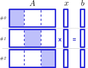
Figure 1: Typical data distribution across the computational processes.

The several issues arise when developing efficient parallel implementation of Krylov subspace iterative methods. Typically the matrix of SLAE and corresponding vectors are divided row-wise into blocks and distributed across the computational processes (Figure 1). This allows to implement vector updates as local operations without any interprocess communications. The sparse matrix-vector multiplication (SpMV) needs some local communications between the neighbour processes, but the time for communications can be overlapped by computations. The third operation, dot product, starts with the computation of the local vector segments dot products, and continues with the global reduction among all computational processes. The global reduction leads to a synchronization point for all computational processes and generally can affect the overall efficiency of the parallel implementation.

Analyzing the BiCGStab method (Algorithm 1 in B) this paper is focused on, one can see that the method has 2 SpMV operations, 6 vector updates and 4 dot products per each iteration. In case of preconditioned method the two preconditioning operations are also performed. Depending on the form of the convergence criteria an additional dot product may be required to perform the convergence check. The further discussion assumes the use of criteria in the form of absolute or relative residual norm, which means the norm of the residual vector $r_{j+1}$ must be additionally computed in line 15 of Algorithm 1. Communications for two dot products in lines 10 and 11 can be merged, which reduces the amount of synchronization points per each iteration of BiCGStab method to 4.

The problem of reducing the communications for the Krylov subspace methods, and specifically the BiCGStab, has received a considerable attention in the literature. The reduction of communications and the increase of the fraction of asynchronous data exchanges are achieved by computations reordering and adding some extra vector operations (vector updates and dot products). This increases the overall computational costs of the methods but reduces the communication overhead in parallel simulations. The extra vector operations are usually ignored when discussing the efficiency of the modified methods as their computational costs are much lower compared to those of SpMV operations. This, however, is not the case when the calculations with multiple right-hand side (RHS) vectors are performed. The input of these operations increases with increasing the number of RHS vectors, which leads to the need of accurate review of the corresponding methods.

Most of the modified methods known to date can be classified in the following categories. The first group of methods focuses on reduction of global synchronization points and grouping together the dot products. The Modified BiCGStab method with two global synchronization points has been proposed in [4], and later the Improved BiCGStab method with the single global synchronization point has been developed [5].

The second group of methods focuses on changing the sequence of computations in order to hide the global communications by the preconditioning operations or sparse matrix-vector multiplications. The Reordered BiCGStab method [6] allows to hide the latency of non-blocking reductions by performing the preconditioning. This becomes possible due to execution of preconditioning in advance, i.e. the preconditioning needed at the next iteration is performed while hiding the global communications at the current iteration. This leads to an additional single preconditioning operation during the solution of SLAE. While the proposed modification allows to hide the global communications, this can provide significant overhead in case of using costly preconditioner and fast convergence rate of the corresponding system. The Pipelined BiCGStab method [7] extends the same idea and rearranges the computations in order to allow hiding the global communications behind both preconditioning and SpMV operation. This makes the method applicable even without preconditioning, but further increases the computational overhead compared to the Reordered BiCGStab method, as an additional advanced SpMV operation is performed. Accounting the different number of extra vector operations for the Reordered and Pipelined BiCGStab methods it becomes tricky to determine a priori the area of applicability for each of the methods together with the classical BiCGStab method.

The third group includes the communication-avoiding BiCGStab methods [8, 9], which combine several SpMV operations and perform the calculation of $s$ iterations an once, thus reducing the amount of local communications. This approach, however, limits the usage of preconditioners by the methods of special form, and also adds some extra operations to reorder the computations.

An additional group of methods, which does not target directly the minimization of communications problem but discusses important implementation aspects of the Krylov subspace methods, includes [10, 11, 12, 13]. The authors of these papers focused their research on implementation of the iterative methods on Graphics Processing Units (GPUs) and demonstrated the role of kernel fusion technique in the performance boost on GPUs. The modifications reducing the amount of kernel launch operations for CG, BiCGStab, and GMRES methods have been proposed. The suggested modifications also reduce the data transfers between the host and device, which produces an additional performance boost.

The papers mentioned above were focused on GPU implementation aspects, and mainly on the single-GPU implementation. The proposed optimizations are valuable for CPU-based computations, but inapplicable “as is” (e.g., the single-GPU implementation in [12, 13] allows to merge the SpMV operation together with the following vector operations, but in multi-device computations the data access to the resulting vector is indirect and can not be efficiently merged with subsequent vector operations). The modifications of the methods proposed in [11] presume the more robust formulation and preserve the sparse matrix-vector multiplication as an independent function call. This decreases the overall performance gain for the loop fusion technique compared the fully fused formulations, but ensures the algorithm does not depend on the matrix storage format and the SpMV operation implementation details.

The current paper attempts to systematically revise the BiCGStab method and several modified versions including the Improved BiCGStab, Reordered BiCGStab and Pipelined BiCGStab in terms of execution time and parallel efficiency with the focus on the computations with multiple right-hand side vectors (the possible convergence issues due to reordering the operations are not accounted in this paper). The rest of the paper is organized as follows. The impact of reducing the amount of data transfers with the memory and merging the vector operations on the performance of BiCGStab methods is discussed in the second section. The third section is devoted to construction of data transfer-based execution time model. The model is applied to the considered BiCGStab methods and validated by the corresponding simulation results. The detailed comparison of the BiCGStab methods is presented in the fourth section. The specifications of compute platforms used for the calculations and merged formulations of the BiCGStab methods are summarized in Appendix.

2 Merging vector operations in BiCGStab methods

2.1 The role of merging vector operations on CPUs

The loop fusion technique applied for GPUs was focused on reduction of data transfers between the host and device memory and decrease of the time losses due to multiple kernel launches. This technique, however, is also of importance for the CPU computations. Merging of several vector operations in some cases allows to reuse the data already transferred from the memory and reduce the total volume of data transfers. Taking into account that the performance of basic operations comprising the iterative methods for solving SLAEs with sparse matrices is limited by the memory bandwidth of the compute system [14], this allows to increase the compute intensity of the algorithm (flop per byte ratio) and, consequently, performance of the calculations.

An importance of the corresponding modifications can be illustrated by the simple example performing the calculation of vector updates: $y=ax+by$, $z=bx+az$, and $z=by+cz$, where $a$, $b$, and $c$ are the scalars and $x$, $y$, and $z$ are the vectors of size $N$. The corresponding operations are computed in three ways: (1) three independent BLAS-like function calls, (2) merged loop performing two vector updates, and (3) merged loop performing three vector updates (Figure 2). The first run needs $9N$ elements to be transferred with the memory and $9N$ floating point operations (FLOP), the second run transfers $5N$ elements and performs $6N$ FLOP, and the last one transfers $5N$ elements with $9N$ FLOP. The corresponding calculation times for the double precision floating point vectors of total length $N=10^{8}$, performed on Lomonosov and Lomonosov-2 compute systems, are shown in Tab. 1 (characteristics of the test platforms can be found in Tab. 7 of A). The presented results are obtained for the single nodes and use MPI with “one rank per core” scheme to utilize all processor cores. One can see the ratio of the execution times to perform the first and second cases is about 1.76. This value is closer to the memory traffic ratio 1.8 than the FLOP ratio 1.5. Moreover, the third case produces the same memory traffic as the second one, but performs 1.5 times as much floating point operations, however, the execution time equals to the second case. This clearly demonstrates that the execution time for these computations depends on the memory traffic but not on the number of floating point operations, and the overhead to compute the third vector update for the data already loaded to the registers is negligible.

⬇

// run #1:

for(i = 0; i < N; i++)

y[i] = a * x[i] + b * y[i];

for(i = 0; i < N; i++)

z[i] = b * x[i] + a * z[i];

for(i = 0; i < N; i++)

z[i] = b * y[i] + c * z[i];

// run #2:

for(i = 0; i < N; i++) {

y[i] = a * x[i] + b * y[i];

z[i] = b * x[i] + a * z[i];

}

// run #3:

for(i = 0; i < N; i++) {

y[i] = a * x[i] + b * y[i];

z[i] = b * x[i] + a * z[i];

z[i] = b * y[i] + c * z[i];

}

Figure 2: Pseudocode of the three groups of vector operations used to analyze the impact of memory traffic on performance of the vector operations.

Table 1: Time to perform vector operations, ms.

	Lomonosov	Lomonosov-2
run #1	207	125
run #2	117	71
run #3	116	71

An observation demonstrated above suggests two conclusions: (1) it is reasonable to reformulate the corresponding iterative methods with the focus on the minimization of memory transfers and grouping vector operations, and (2) the execution time model must include the metrics based on the volume of data transfers, but not the floating point operations.

2.2 Merged formulations of BiCGStab iterative methods

The simple example presented in the previous paragraph clearly shows importance of merging the vector operations in Krylov subspace methods to achieve maximal performance. The current paragraph provides the merged formulations for the modified BiCGStab methods discussed in the rest of the paper. It should be noted the applicability of the approach considered is not limited by the chosen group of methods and can also be applied to the other iterative methods.

The following principles make the basis of constructing the merged formulations of the methods. The merging of vector operations is applied if:

• merging does not increase the amount of communications and overall computational costs of the method (i.e., no extra computations allowed after the convergence criteria satisfied);

• merging does not decrease the amount of computations that can be used to hide the asynchronous communications;

• merged operation reduces the number of vector reads/writes.

In contrast with GPU computations, CPUs do not have observable penalty on additional function calls, and reduction of overall function calls has negligible impact on the overall performance.

Considering the BiCGStab method presented in Algorithm 1 in B, three groups of merged vector operations are suggested. Grouping of three dot products in line 9 of Algorithm 2 in B, needed to compute the coefficient $\omega_{j}$ and norm of the residual vector $r_{j+1}$, allows to reduce the memory traffic from six vector reads to only two. Grouping of two vector updates in line 12 allows to reduce single vector read operation (this branch, however, is executed only once and has little effect on the overall performance). Finally, grouping in line 15 allows to reduce two vector reads. In total, the memory traffic for the single loop of the BiCGStab method decreases from 18 read and 4 write operations to 14 reads and 4 writes in the merged formulation.

Applying the same principles to the modified BiCGStab methods one can obtain the merged formulations for these methods. The corresponding algorithms are presented in B and the data traffic characteristics of the proposed formulations are summarized in Tab. 2. While merging of vector operations for classical BiCGStab method allows to reduce data traffic for vector operations by only 18% and this value is even lower for the preconditioned method, the effect of merging is much stronger for the modified formulations: for Improved BiCGStab and Pipelined BiCGStab methods the data traffic can be decreased twofold. Merging of vector operations allows to significantly reduce the overhead occurred as a result of reordering the computations to decrease the communication costs.

Table 2: Number of vector read/write operations per single iteration of the iterative method.

Method	Basic			Merged
	Read	Write	Total	Read	Write	Total
BiCGStab	18	4	22	14	4	18
IBiCGStab	27	6	33	14	6	20
PipeBiCGStab	34	9	43	18	8	26
PBiCGStab	18	4	22	15	4	19
RBiCGStab	22	6	28	15	6	21
PPipeBiCGStab	43	13	56	23	11	34

2.3 Numerical experiments

The presented theoretical prepositions are validated by the numerical simulation results. The corresponding algorithms are implemented in a newly developing XAMG library of numerical methods for solving SLAEs with multiple RHS vectors. The testing is done for the matrix obtained as a result of spatial discretization of the Poisson equation in a cubic domain using 7-point stencil with the uniform grid of $200^{3}$ cells and single RHS vector (of 8 mln. unknowns). The fixed number of iterations is used for the benchmark purposes, $N_{it}=1000$, to measure the corresponding execution time. The simulations are performed on the single compute node and utilize all available processor cores; the computations are parallelized with help of MPI, mapping one MPI rank per each processor core. In case of preconditioned methods the identity operator is used as a preconditioner, which leads to a simple vector copy, equivalent in terms of data traffic to a single vector read and write operations (the preconditioning costs are not included in Tab. 2).

The testing is performed for six iterative methods including classical BiCGStab, Improved BiCGStab, Pipelined BiCGStab, preconditioned BiCGStab, Reordered BiCGStab and preconditioned Pipelined BiCGStab methods for both basic and merged formulations. The corresponding execution times are summarized in Tab. 3. The classical BiCGStab method demonstrates the lowest execution time. The Improved BiCGStab takes 20% more time for basic formulation and 7% for the merged one. The Pipelined BiCGStab has overhead of about 40%, but thanks to merging of vector operations it can be reduced twofold.

The preconditioned BiCGStab is also the fastest among the preconditioned methods. The Reordered BiCGStab shows 7% overhead, and it becomes as small as 2% with the merged formulation. The preconditioned Pipelined BiCGStab slows down by 60%, but this value can also be reduced twofold if using merged formulation of the method.

The presented results demonstrate that merging of vector operations is a useful optimization for CPU computations allowing to decrease the calculation time by reducing the data traffic. The execution time reduction varies depending on the method from 4% to 21%. The proposed optimization decreases the computational costs to perform extra vector operations introduced as a result of reordering thus allowing to extend the range of applicability of modified methods.

The efficiency of the implemented methods is compared with the open-source hypre [16] library (hypre v.2.15.1 has been built with Intel compiler and Intel MKL, and with MPI and OpenMP parallelization). The measured execution times for the unpreconditioned BiCGStab method are up to 20% higher than the ones obtained with the current implementation of basic BiCGStab method formulation. Compared the merged formulations the overall speedup reaches 36% and 28% for Lomonosov and Lomonosov-2 supercomputers correspondingly.

Table 3: Execution times for the single iteration of the numerical method, times in ms.

Method	Lomonosov		Lomonosov-2
	Basic	Merged	Basic	Merged
BiCGStab	113	105	61.5	57.5
IBiCGStab	136	113	74.3	61.2
PipeBiCGStab	157	126	86.5	68.6
PBiCGStab	121	116	66.4	63.7
RBiCGStab	129	117	72.1	64.8
PPipeBiCGStab	195	155	107	84.8
hypre, BiCGStab (MPI)	143	–	81.8	–
hypre, BiCGStab (MPI+OpenMP)	144	–	74	–

The effect of merging vector operations for the simulations with multiple RHS vectors is demonstrated in Tab. 4. Using the same test matrix, the series of experiments are repeated for SLAEs with 4 and 16 RHS vectors. The obtained results show the increase of the merging effect when performing simulations with multiple RHS vectors, and the higher a method is affected by vector merging, the stronger an effect appears to be. While the classical BiCGStab shows increase by only 3%, the use of vector merging for the Pipelined BiCGStab allows to accelerate the simulations with 16 RHS vectors by 27%.

Table 4: Execution times and corresponding improvement due to merging of vector operations for the single iteration of the numerical method with variable number of RHS vectors. Lomonosov-2 supercomputer, times in seconds.

Method	$m=1$			$m=4$			$m=16$
	Basic	Merged	Imp.	Basic	Merged	Imp.	Basic	Merged	Imp.
BiCGStab	0.062	0.058	7%	0.181	0.164	9%	0.65	0.59	10%
IBiCGStab	0.074	0.061	18%	0.236	0.182	23%	0.87	0.66	25%
PipeBiCGStab	0.087	0.069	21%	0.282	0.212	25%	1.06	0.78	27%
PBiCGStab	0.066	0.064	3%	0.201	0.189	6%	0.72	0.68	7%
RBiCGStab	0.072	0.065	10%	0.224	0.196	12%	0.81	0.7	14%
PPipeBiCGStab	0.107	0.085	21%	0.368	0.279	24%	1.39	1.03	26%

3 Execution time model

A variety of modifications of numerical methods published in the literature leads to the need of formulating simplified models to classify them and highlight the range of applicability for each of the methods. The corresponding attempts to construct analytical models have been done earlier, e.g., in [17, 18]. The basic execution time model has been proposed in [17]. The model includes the time to perform the floating point operations and the time of global communications for dot products, but ignores the time spent on SpMV communications. Using this model the authors proposed parallel modifications of CG and GMRES methods, focused on reduction of global communications and hiding communications by local computations.

The corresponding model has been revised and applied to Generalized Product type of Bi-Conjugate Gradient method [19, 20] in [18]. This model is also based on the amount of floating point operations and accounts the time spent on data exchanges in SpMV operations and dot product calculations. The corresponding communication time dependencies on the number of processes are expressed as a power functions, and the free parameters are calibrated with results of numerical experiments.

The major drawback of these models relies in the usage of floating point operations as a metric of the execution time. As shown in the previous section, the basic operations in Krylov subspace methods applied to solve large sparse SLAEs are memory bound and limited by the memory bandwidth, but not by the compute capacity of modern processors. Thus, the execution time for the operations is determined by the amount of data to be read from and written to the memory, but not by the corresponding floating point operations.

3.1 Data transfer-based execution time model

The data transfer-based execution time model is constructed to analyze the efficiency and range of applicability for various BiCGStab methods. The model covers simulations with multiple RHS vectors and additionally allows to account various preconditioners. It is assumed multiple vectors are stored row-wise in a single vector, allowing to improve the cache data reuse when performing SpMV operations and utilize the vectorization effects. The minimal compute unit in the analytical model is chosen equal to the single compute node.

The execution time for the single iteration loop of the BiCGStab methods includes the times to perform local vector operations, $T_{vec}$, global data exchanges when calculating dot products, $T_{G}$, sparse matrix-vector multiplications, $T_{mul}$, and communications with local neighbours when computing SpMVs, $T_{L}$. In case of preconditioned methods, an additional time spent on preconditioning, $T_{prec}$, must be included. The time for local calculations can be expressed as a ratio of the volume of data transfers, $\Sigma$, to the compute system memory bandwidth, $B$:

$$T=\frac{\Sigma}{B},$$ (1)

where the overall memory bandwidth is a multiplication of the memory bandwidth of the single node, $b$, to the number of compute nodes, $p$, used in the calculations:

$$B=b\,p.$$ (2)

Assuming the integers and floating point numbers are of size 4 and 8 bytes respectively, and the sparse matrix is stored in CRS format [21], the corresponding sparse matrix-vector multiplication needs [22]

$$\Sigma_{mul}=N\left(8m(C+1)+4(3C+1)\right)$$ (3)

bytes to be transferred with the memory. Here, $N$ is the matrix size, $m$ is the number of RHS vectors, and $C$ denotes the average number of nonzeros per matrix row. This leads to the SpMV local computations execution time

$$T_{mul}(p)=\frac{N\left(8m(C+1)+4(3C+1)\right)}{b\,p}.$$ (4)

The memory traffic of single vector read/write operation is expressed as

$$\Sigma_{vec}=8\,N\,m.$$ (5)

Substituting this expression to (1), the estimate for the vector operations execution time takes the form:

$$T_{vec}(p)=\frac{8Nm}{b\,p}.$$ (6)

To complete, the local and global communication times as a functions of the number of compute nodes and message size must be provided.

3.1.1 Local communications

The local non-blocking point-to-point communications arise when performing data exchange to complete the SpMV operation. Generally, the communication pattern (list of neighbour processes and message sizes) depends on a couple of factors including the matrix topology and data decomposition, and construction of the corresponding time estimates can be a challenging issue. In order to simplify the further narration and focus on the effect of global communications the specific form of the test matrices is considered for parallel runs. The case assumes the communication pattern remains close to constant with increasing the number of compute processes. Such a scenario is realized, for example, for banded matrices with narrow band.

The corresponding communication pattern can be modelled with the simple benchmark, performing asynchronous data exchange for each process with only several neighbours. This test is a generalization of IMB Exchange benchmark [23], which allows to measure the latency of the non-blocking point-to-point communications depending on the number of neighbours and transferred message size. The testing is performed on Lomonosov supercomputer using up to 128 compute nodes and 8 MPI processes per node. The obtained results show that the time to transfer the data is almost independent on the overall number of MPI processes and weakly depends on the number of neighbours if it does not exceed 10. The local communications time can be expressed as a function of the transferred message size in the form

$$T_{L}(l)=C_{0}+C_{1}\,l^{n_{0}},$$ (7)

where $l$ is the message size in bytes. The corresponding data fitting of the benchmark results gives two sets of coefficients depending on the message size:

$$T_{L}(l)=\begin{cases}2.4\cdot 10^{-6}+6.9\cdot 10^{-8}\,l^{0.56}&,\,l\leq 2048\,\,\mbox{bytes},\\ 3.2\cdot 10^{-6}+2\cdot 10^{-9}\,l&,\,l>2048\,\,\mbox{bytes}.\end{cases}$$ (8)

3.1.2 Global communications

The need for global communications arise after performing the dot products with local vector fragments. The corresponding operation using the MPI library to perform communications can be implemented in the form of blocking call of MPI_Allreduce or non-blocking call of MPI_Iallreduce function. Theoretically, the second one can be preferable for the algorithms with overlap of global communications by computations (e.g., the Reordered BiCGStab or Pipelined BiCGStab methods). In practice, however, the situation is not so evident. The efficiency of the non-blocking global communications depends on lots of factors, including the MPI library implementation and communications hardware. To perform the non-blocking collective operations (e.g., MPI_Iallreduce) the specific progression must be applied. The MPI standard [24] does not specify the progression rule, and its implementation varies depending on the specific MPI library [25]. Three basic progression strategies are discussed in the literature [26]: hardware-based progression, software-based progression, and manual progression. The first option seems to be the most promising one, but is available in a limited number of compute systems (e.g., Cray systems with Gemini or Aries interconnect [25]), and not fully supported in the majority of other systems. The software based progression is implementation-specific, and not limited by the communication hardware. This option is typically implemented with threads, which handle the status of the non-blocking operations and perform the corresponding progression. The drawback for this strategy is related with significant overhead, produced by the progression threads [26, 27, 28, 29]. The manual progression is generally independent on the hardware and MPI library implementation, but needs some user efforts to add MPI_Test or MPI_Probe calls to progress the communications. Each of the strategies mentioned above has its advantages and disadvantages depending on the performed communication and message size. The corresponding discussion can be found in, e.g. [25, 26, 27, 28, 29].

The efficiency of global communications and various progression techniques for the Lomonosov supercomputer has been investigated in detail with help of corresponding benchmark in C. The efficiency of overlap of communications and computations is estimated in terms of overlapping overhead, $\gamma$. This parameter is defined as

$$\gamma=\frac{T_{calc}^{async}+T_{comm}^{async}-T_{calc}^{sync}}{T_{comm}^{sync}},$$ (9)

where $T_{calc}$ is the calculation time and $T_{comm}$ is the time spent on communications. Superscripts “sync” and “async” correspond to blocking synchronous and non-blocking asynchronous communications respectively; $T_{calc}^{async}$ can be higher than $T_{calc}^{sync}$ due to influence of communications performing in background with calculations (the details can be found in C). The parameter introduced characterizes the degree of overlap of communications by computations with account of potential increase of the calculation time due to progress of asynchronous non-blocking communications.

The presented results demonstrate that the special efforts are needed to obtain the overlap of non-blocking global communications by computations. The experiments with Intel MPI 2017 library have shown that, while the software progression provides almost ideal overlap with overlapping overhead of only 10-20%, the execution times for the global reductions with short messages (less than 8192 bytes) increase more than by the order of magnitude compared the ones without software progression. This makes the corresponding functionality inapplicable in real simulations. The manual progression allows to obtain overlapping overhead by about 30-50%, however, it requires to perform systematic MPI_Test progression calls and it can be tricky to implement this progression in real computational codes.

The simple analytical expression for blocking global communications can be constructed as a result of generalization of benchmark results presented in C. Following [18], the power function is used to approximate the measured data. It is found the measured data can be approximated with acceptable degree of accuracy by the function

$$T_{G}(p,l)=C_{0}+C_{1}\,l^{n_{0}}\,p^{n_{1}},$$ (10)

where the message size $l$ is equal to $l=8\,m\,k$, and $k$ is the number of dot products computed at once. For the iterative methods considered in the paper this parameter varies from 1 to 7. The corresponding coefficients $C_{0}$, $C_{1}$, $n_{0}$, and $n_{1}$ are defined by fitting results of numerical experiments. For Lomonosov supercomputer these coefficients are equal to:

$$C_{0}=3.5\cdot 10^{-6},\,C_{1}=1.7\cdot 10^{-6},\,n_{0}=0.21,\,n_{1}=0.54.$$ (11)

The overlapping overhead parameter, $\gamma$, is used to account the degree of overlap when performing asynchronous global communications. The corresponding execution time for the calculations and non-blocking asynchronous communications takes the form:

$$T=\max(T_{calc}+\gamma T_{G},T_{G}).$$ (12)

3.1.3 Execution times for the BiCGStab methods

Using the expressions introduced above one can obtain the expected execution times for the iterative methods. The corresponding relations presented below operate with merged formulations of the methods with reduced number of vector reads/writes. The classical BiCGStab method performs all the calculations step-by-step, except the calculation of sparse matrix-vector multiplication and local communications, which can be efficiently overlapped. This leads to the following form of the theoretical execution time for the single iteration of the BiCGStab method:

$$T^{BiCGStab}(p)=18T_{vec}(p)+2T_{SpMV}(p)+T_{G}(p,24m)+\\ 2T_{G}(p,8m),$$ (13)

where

$$T_{SpMV}(p)=\max\left(T_{mul}(p),T_{L}(l)\right)$$ (14)

and $l$ is the average message size transferred with the neighbour processes. Opposite to the global communcations, it is assumed that local non-blocking asynchronous point-to-point communications do not produce observable overlapping overhead [30] and this overhead is ignored in the analytical model. The real average message size depends on the specific test matrix and the corresponding data distribution across the compute processes. For the sake of simplicity, in the following discussion the message size is assumed independent on the number of compute processes utilized. This assumption is valid for the test matrix used in the following validation section. Meanwhile, the corresponding dependence can be included without in due difficulties to the proposed execution time model.

The Improved BiCGStab method generally has the same structure of the algorithm as the classical method formulation with the only difference in the number of vector operations and global communications:

$$T^{IBiCGStab}(p)=20T_{vec}(p)+2T_{SpMV}(p)+T_{G}(p,56m).$$ (15)

The message size for the global communications in the Improved BiCGStab is about twice higher than the ones in the classical BiCGStab method, but changed order of computations allows to decrease the number of global reductions, which is typically preferable in the high-scale simulations. The Pipelined BiCGStab method allows to hide the global communications by the SpMV operation. Accounting the overlap of global communications and computations, the following relation for the execution time can be formulated:

$$T^{PipeBiCGStab}(p)=26T_{vec}(p)+\\ \max\left(T_{SpMV}(p)+\gamma T_{G}(p,24m),T_{G}(p,24m)\right)+\\ \max\left(T_{SpMV}(p)+\gamma T_{G}(p,32m),T_{G}(p,32m)\right).$$ (16)

The preconditioned methods reproduce the same sequence of computations and additionally perform two preconditioning operations per each iteration of the methods. For the preconditioned BiCGStab method the corresponding times are not overlapped with any computations and simply added to the overall execution time:

$$T^{PBiCGStab}(p)=19T_{vec}(p)+2T_{SpMV}(p)+2T_{prec}(p)+T_{G}(p,24m)+\\ 2T_{G}(p,8m).$$ (17)

The Reordered BiCGStab method allows to overlap preconditioning operations with global reductions. Using expression (12) the corresponding expression takes the form:

$$T^{RBiCGStab}(p)=21T_{vec}(p)+2T_{SpMV}(p)+\\ \max\left(T_{prec}(p)+\gamma T_{G}(p,8m),T_{G}(p,8m)\right)+\\ \max\left(T_{prec}(p)+\gamma T_{G}(p,32m),T_{G}(p,32m)\right).$$ (18)

Finally, the preconditioned Pipelined BiCGStab method allows to overlap global communications with preconditioning and sparse matrix-vector multiplication:

$$T^{PPipeBiCGStab}(p)=34T_{vec}(p)+\\ \max\left(T_{SpMV}(p)+T_{prec}(p)+\gamma T_{G}(p,24m),T_{G}(p,24m)\right)+\\ \max\left(T_{SpMV}(p)+T_{prec}(p)+\gamma T_{G}(p,32m),T_{G}(p,32m)\right).$$ (19)

3.2 Execution time model validation

The proposed execution time model is thoroughly validated and compared with the corresponding calculation results. Validation includes the single-node runs, performed on two compute systems, and multi-node runs, performed on 128 compute nodes of Lomonosov supercomputer.

3.2.1 Single-node validation

The single-node validation is performed for the test matrix of 8 mln. unknowns, previously used in section 2.3. This test series includes the runs performed for the merged formulations of the methods with 1, 4, and 16 RHS vectors on the Lomonosov and Lomonosov-2 supercomputers. In case of preconditioned methods the identity operator is used as a preconditioner, which is equal to single vector copy operation. While the parallelization inside the node is implemented using MPI, the overhead due to communications for the chosen test matrix is negligible compared the overall execution time, and results of the comparison mostly validate correctness of the estimates for the computational operations.

The obtained calculation results for all the methods considered in the paper together with the predicted execution times are presented in Tab. 5 and Tab. 6 (results for the Lomonosov supercomputer include only 1 and 4 RHS vector calculations due to compute node memory limitations). The memory consumption to store the data for this test case is measured by several gigabytes, which allows to suggest the use of memory bandwidth of the random-access memory (RAM) as a data transfer bandwidth model estimation. The presented results demonstrate good correspondence of the theoretical and measured execution times for both compute systems. The analytical model slightly underpredicts execution time for the Pipelined BiCGStab method, providing the deviation by approximately 12%. The difference for all other test cases is within 5%. The obtained predictivity is supposed to be acceptable for the comparison purposes stated in the current paper.

Table 5: Predicted and measured execution times of the single iteration loop for the BiCGStab methods with variable number of RHS vectors. Lomonosov supercomputer, times in seconds.

Method	$m=1$		$m=4$
	Model	Real	Model	Real
BiCGStab	0.106	0.107	0.3	0.29
IBiCGStab	0.109	0.113	0.32	0.32
PipeBiCGStab	0.12	0.127	0.36	0.38
PBiCGStab	0.115	0.116	0.34	0.33
RBiCGStab	0.119	0.117	0.35	0.34
PPipeBiCGStab	0.143	0.156	0.45	0.49

Table 6: Predicted and measured execution times of the single iteration loop for the BiCGStab methods with variable number of RHS vectors. Lomonosov-2 supercomputer, times in seconds.

Method	$m=1$		$m=4$		$m=16$
	Model	Real	Model	Real	Model	Real
BiCGStab	0.057	0.058	0.16	0.16	0.59	0.58
IBiCGStab	0.059	0.061	0.17	0.18	0.62	0.64
PipeBiCGStab	0.065	0.069	0.19	0.21	0.71	0.76
PBiCGStab	0.062	0.064	0.18	0.19	0.66	0.69
RBiCGStab	0.064	0.065	0.19	0.19	0.7	0.69
PPipeBiCGStab	0.077	0.085	0.24	0.27	0.9	1.01

3.2.2 Multi-node validation

Following [7, 18] the multi-node validation is performed for the test matrix, obtained as a result of discretization of 2D problem. The matrix of 1 mln. unknowns, corresponding to the grid of $1000^{2}$ cells and 5-point stencil is used in the tests. The native ordering allows to obtain almost constant communication overhead for the SpMV operation in the range up to $10^{3}$ compute processes, thus allowing to evaluate the impact of global communications on the overall methods execution time. The suboptimal data decomposition for the general matrices can be obtained using the graph partitioning algorithms (e.g., [31, 32]). This, however, lies beyond the scope of this paper.

Expressions (13)-(19) allow to predict the expected execution times for the single iteration of the numerical methods depending on the number of compute nodes and RHS vectors. The only ambiguous parameter in the estimates is the memory bandwidth. Analytical expressions allow to cover two limiting cases expecting the data is loaded from the RAM or the data is loaded to the registers from the last level cache. The corresponding predictions for the BiCGStab method with single RHS vector are presented in Figure 3. Starting with about 3.7 times difference for the single node runs, these curves become closer with increasing the number of compute nodes involved in the calculations. At the scale of $10^{2}$ nodes (800 processes) the scalability reaches saturation, and predicted times become almost identical for both configurations, which indicates domination of communications over computations.

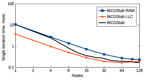
Figure 3: Analytical predictions and numerical simulation results for the classical BiCGStab method.

The measured execution times for the BiCGStab method fit the range between the two analytical curves. Computations with 1–4 nodes provide results corresponding to the RAM bandwidth predictions. The further increase in the number of compute nodes allows to decrease the memory consumption per node and improve the cache reuse. Starting from several tens of nodes the data fits the cache, which leads to a reduction in the execution time and shift of the calculation results towards the LLC predictions.

The paper [7] contains execution time results for 1 mln. 5-diagonal test matrix, performed on the hardware platform very similar to the one used for the validation in the current paper (InfiniBand QDR interconnect, compute nodes with 2 x 6-core Intel Xeon X5660 processors) with only minor difference in the number of processor cores per node. To compare the model predictions and simulation results together with results of other authors the execution times for the single iteration of basic formulations of classical BiCGStab and Pipelined BiCGStab methods are summarized in Figure 4. The present simulation results demonstrate good agreement with analytical model predictions for both iterative methods. The obtained results significantly outperform the ones presented in [7]. The newly developed implementation of the methods provides 1.8 and 2.4 times lower execution times for the single-node runs of classical BiCGStab and Pipelined BiCGStab methods correspondingly.

The poor scalability of the methods for the considered test matrix is demonstrated in [7]. The speedup, defined as a ratio of the execution time on the single node to the one with $p$ nodes,

$$S(p)=\frac{T(1)}{T(p)}.$$ (20)

does not exceed 3.5 for the classical BiCGStab, and for the Pipelined BiCGStab it reaches 15.5. The present results, to the contrary, demonstrate the superlinear speedup (Figure 5). This effect is a result of cache usage improvement, which allowed more than 35-fold decrease of the execution time on 20 compute nodes. In total, the current implementation of the iterative methods outperforms results of [7] for the classical BiCGStab by a factor of 20, and for the Pipelined BiCGStab by a factor of 7.8. While the paper [7] shows advantage of the Pipelined BiCGStab method starting from 4 compute nodes, the present results do not reproduce this behaviour. The classical method outperforms the pipelined variant in the whole range of the compute nodes considered in this test.

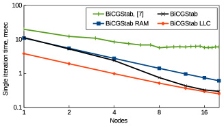
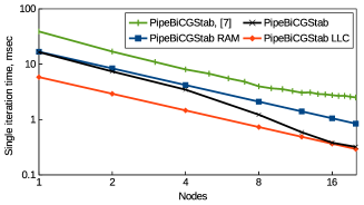
Figure 4: Comparison of execution times for the basic formulations of classical BiCGStab and Pipelined BiCGStab methods with results presented in [7].

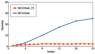
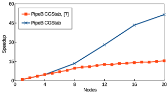
Figure 5: Scalability of basic formulations of classical BiCGStab and Pipelined BiCGStab methods compared with results presented in [7].

4 Comparison of modified BiCGStab methods

The above presented results of the analytical model validation demonstrate good correspondence of predictions and calculations. This allows to use the proposed model to investigate the influence of various parameters on the execution times of the methods and indicate the range of applicability for each of the iterative methods considered in the paper.

4.1 Model predictions

The range of applicability for the modified BiCGStab methods can be estimated by analysing expressions (13)-(19). The modified methods allow to decrease the number of global reductions by the price of several extra vector operations and hide the communications by computations. The typical scale of the problem per each compute node when the modified method can outperform the classical one can be estimated as:

$$T_{G}\sim\frac{8Nm}{bp}.$$ (21)

Using the reference values for global reduction of 20 $\mu$s and LLC memory bandwidth of $10^{11}$ bytes/s, one can obtain the estimate $Nm/p\sim 2.5\cdot 10^{4}$ elements per node, and this value further decreases with increasing the number of RHS vectors.

The further analysis of the range of optimality for the numerical methods is performed with help of the following parameter:

$$R^{i}(p)=\frac{\min_{j\in K}\left(T^{j}(p)\right)}{T^{i}(p)},\,i\in K,$$ (22)

which can be interpreted as a relative performance of the specific method among the set of the methods considered. Here, $K$ is the set of the iterative methods, i.e. K = {BiCGStab, IBiCGStab, PipeBiCGStab} or K = {PBiCGStab, RBiCGStab, PPipeBiCGStab}. This parameter varies in the range $R^{i}\in(0,1]$ and shows how close is the specific method to the optimal numerical method providing the minimal execution time. The proposed estimates (13)-(19) allow to plot the corresponding distributions depending on various model parameters as a functions of the number of compute nodes. These plots clearly show the range of optimality for each of the considered methods.

The plots, presented in Figure 6, allow to compare the efficiency of the numerical methods when solving system of linear algebraic equations with single RHS vector, and indicate the influence of overlapping of global communications with computations. The lowest execution times at the scale of 1–10 compute nodes among the unpreconditioned methods are observed for the classical BiCGStab method. The Improved BiCGStab has about 5% penalty and the Pipelined BiCGStab demonstrates about 15% relative performance degradation. The Improved BiCGStab outperforms two other methods at the scale of 10–30 compute nodes due to only single global reduction performed at each iteration compared to three global reductions needed by the classical BiCGStab and two global reductions of the pipelined method. The choice of the optimal method at the higher scales of compute nodes varies depending on the overlap parameter $\gamma$. In case of no overlap ($\gamma=1$) the Improved BiCGStab remains the optimal method in the range of compute nodes considered. The partial overlap ($\gamma=0.5$) improves the characteristics of the Pipelined BiCGStab method, and at the scale of 100 nodes it provides the execution times compatible with the Improved BiCGStab. Finally, the full overlap ($\gamma=0$) allows to unleash the potential of the Pipelined BiCGStab method. This method provides the highest performance in the range of 30–250 compute nodes.

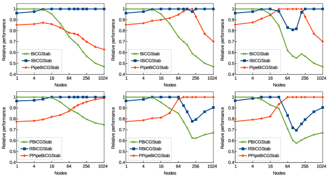
Figure 6: Relative performance of iterative methods when solving SLAE with single RHS vector depending on degree of overlap of communications and calculations. From left to right: no overlap, $\gamma=1$; partial overlap, $\gamma=0.5$; full overlap, $\gamma=0$.

In case of using the lightweight preconditioner (the computational complexity of the preconditioner, $\alpha$, equal to two vector reads/writes) the classical BiCGStab is also the optimal method at the scales of 1–10 nodes. The Reordered BiCGStab outperforms the classical BiCGStab method at the scales of 10–50 compute nodes due to reduced number of global reductions. The preconditioned Pipelined BiCGStab has the same number of global reductions, but significantly higher number of vector operations, thus demonstrating lower performance compared the Reordered BiCGStab. In case of at least partial overlap of global communications by computations the pipelined method can outperform two other methods starting from 50–100 compute nodes. Its performance, however, strongly depends on the overlap parameter, $\gamma$.

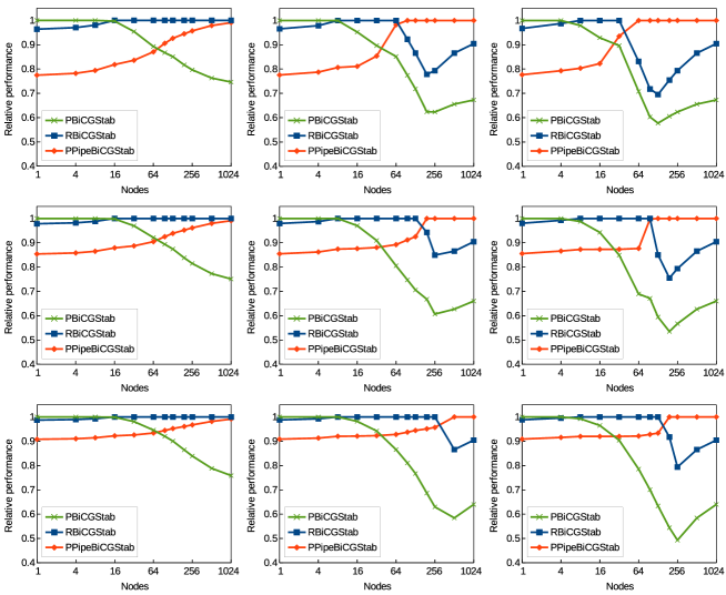
Figure 7: Influence of preconditioner complexity on the performance of iterative methods. From left to right: no overlap, $\gamma=1$; partial overlap, $\gamma=0.5$; full overlap, $\gamma=0$. From top to bottom: no preconditioner, $\alpha=2$; $\alpha=20$; $\alpha=50$.

The preconditioner complexity does not have principal influence on the methods relative performance (Figure 7). The increase of the preconditioner complexity shifts towards the higher scales the transition point from the Reordered BiCGStab to the Pipelined BiCGStab and reduces the difference in the relative performance of the methods. The latter one is caused by a reduction of the role of extra vector operations in the overall computational costs.

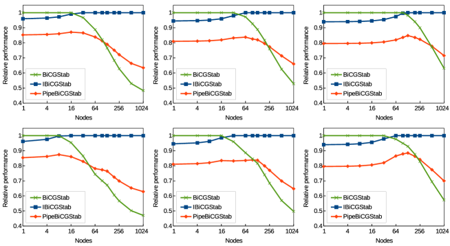
Figure 8: Relative performance of the iterative methods for SLAEs with multiple RHS vectors, unpreconditioned methods. First row – RAM memory bandwidth estimates; second row – LLC memory bandwidth estimates. From left to right: $m=1$; $m=4$; $m=16$.

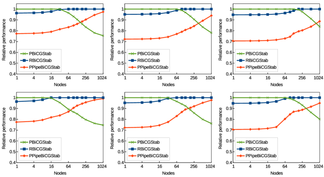
Figure 9: Relative performance of the iterative methods for SLAEs with multiple RHS vectors, preconditioned methods. First row – RAM memory bandwidth estimates; second row – LLC memory bandwidth estimates. From left to right: $m=1$; $m=4$; $m=16$.

The increase in the number of RHS vectors increases the memory consumption and a fraction of vector operations in the overall execution time. The first aspect leads to the increase in the number of compute nodes when the data starts to fit the cache. While for the single RHS vector the cumulative LLC memory of about 15 compute nodes of Lomonosov supercomputer is enough to store the data, for 4 and 16 RHS vectors this value increases to 30 and 100 nodes correspondingly. This indicates that the expected transition points for the simulations with 4 RHS vectors would be in between of analytical model predictions with RAM and LLC memory bandwidth, and results for 16 RHS vectors would mostly correspond to the RAM bandwidth values.

The analytical model predictions for 1, 4, and 16 RHS vectors with RAM and LLC memory bandwidths are summarized in Figures 8-9. The plots indicate that the increase in the amount of RHS vectors for the unpreconditioned methods (Figure 8) leads to a systematic shift of the transition point from the classical BiCGStab to the Improved BiCGStab towards the higher scales in compute nodes. The Pipelined BiCGStab demonstrates at least 20% higher execution times compared to the other methods in the whole range of compute nodes considered.

The similar situation is observed for the preconditioned methods (Figure 9): the preconditioned Pipelined BiCGStab demonstrates about 30% higher execution times and this value decreases only at the scale of thousands of compute nodes. The Reordered BiCGStab method can be beneficial compared the preconditioned BiCGStab method starting from the scales of 32–128 compute nodes, and this transition point also shifts to the right along the compute nodes axis with increasing the number of RHS vectors.

The proposed analytical model allowed to compare execution times of the BiCGStab methods and identify the influence of various parameters. The estimates presented above cover the range of compute nodes from 1 to 1024. Accounting the size of the test problem and the specific form of the local communications time function, which is generally valid up to 1000 compute processes (about 120 compute nodes of the current test platform), it should be noted that practical range of these estimates is limited by 128 nodes. To be able to predict correctly the execution times at the higher scales, the more complicated local communication time function must be applied.

4.2 Validation of model predictions with simulation results

The current section focuses on validation of results obtained using the proposed analytical execution time model. The validation starts with investigation of the single iteration execution times when solving SLAEs with 1, 4, and 16 RHS vectors for the methods considered in the paper. The corresponding experiments are performed for the merged formulations of the methods in the range of 1–128 compute nodes and utilize all available 8 cores per each node. This test series do not assume any special manipulations with progression of non-blocking global communications. Accounting results of the corresponding benchmark, presented in C, no overlap of communications is expected.

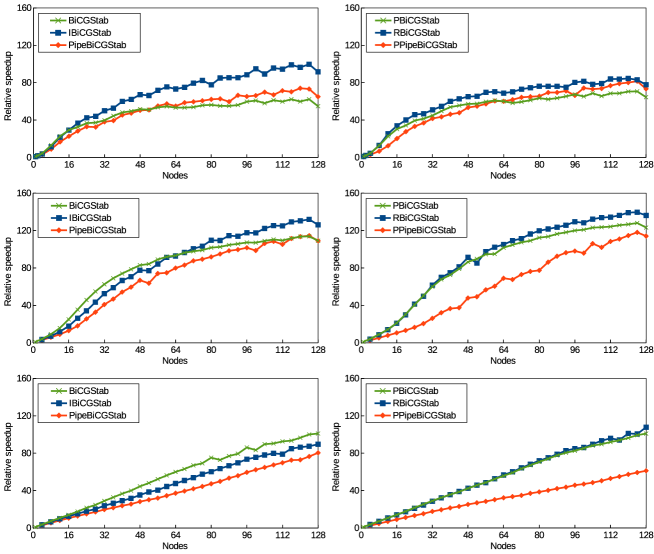
Figure 10: Relative scalability of the methods when solving SLAEs with multiple RHS vectors. From top to bottom: $m=1$; $m=4$; $m=16$.

The measured simulation results in the form of relative speedup are presented in Figure 10. This parameter is defined as a ratio of the execution time for the classical BiCGStab method (or the preconditioned one) when performing simulation on the single compute node to the execution time of the specific method with $p$ compute nodes:

$$P^{i}(p)=\frac{T^{(P)BiCGStab}(1)}{T^{i}(p)}.$$ (23)

The presented plots demonstrate good correspondence with the analytical model predictions for the case with no overlap of global communications ($\gamma=1$). The analytical model correctly predicts the scales of compute nodes corresponding to the transition points. Simulations with single RHS vector confirm predictions in that the optimal methods for the scales of 1–10 compute nodes is the classical BiCGStab, and for the higher scales – Improved BiCGStab or Reordered BiCGStab among the unpreconditioned and preconditioned methods correspondingly. For the unpreconditioned methods the Improved BiCGStab becomes the optimal method for the simulations with 4 RHS vectors starting from about 64 nodes while for the lower scales the classical BiCGStab demonstrates the best performance. The further increase of the amount of RHS vectors increases the role of extra vector operations and moves the transition point between the classical BiCGStab and the Improved BiCGStab beyond the scale of 128 nodes. While the Pipelined BiCGStab has high potential for large scale simulations, the overlap of global communications by computations is a prerequisite to unleash all the advantages of this method. The absence of overlap of global communications, however, does not allow to demonstrate advantages of the Pipelined BiCGStab method in practice.

The preconditioned BiCGStab and Reordered BiCGStab methods demonstrate about the same relative scalability results, with minor advantage of classical method at the lower scales and of Reordered BiCGStab at the higher scales. The performance variation, however, is only within several percent. The preconditioned Pipelined BiCGStab provides significantly higher execution times, which is a result of higher number of extra vector operations occurred as a result of algorithm reordering.

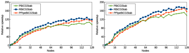
Figure 11: Relative scalability of the methods with various preconditioner complexity when solving the SLAE with single RHS vector. Left – $\alpha=20$; right – $\alpha=50$.

The second validation case investigates the influence of the preconditioner complexity on the relative speedup of the methods. The corresponding runs are performed for the group of preconditioned methods and two preconditioners with complexity equal to 20 and 50 vector read/write operations. The obtained scalability results demonstrate similar behaviour for both configurations with only the difference in the maximal values (Figure 11). The increase in the preconditioner complexity leads to an increase in the peak scalability values by a factor of 1.5. The methods optimality intervals correspond to the ones obtained as a result of analytical model predictions.

Presented above simulation results and results in C demonstrate that progression of global non-blocking operations is not automatically performed during the calculations on the compute system used in the parallel runs. Lomonosov supercomputer has no hardware support for the non-blocking collective operations, and the use of software progression, implemented in the Intel MPI library with specialized progression threads, leads to significant performance degradation, even though it provides the expected communications overlap. This fact makes corresponding functionality inapplicable for the real simulations. As an alternative, the manual progression is investigated in the following series of numerical experiments. The scalability for the merged formulations of Reordered BiCGStab and preconditioned Pipelined BiCGStab methods with manual progression is investigated in the range of 1–128 compute nodes. The preconditioner is emulated in the form of a loop over a set of vector operations, and the MPI_Test calls are performed after each vector operation. The preconditioners with complexity of 20 and 50 vector read/write operations are considered, i.e. 10 and 25 MPI_Test calls can be performed to progress global reduction. For the pipelined method additional MPI_Test calls are also performed during the SpMV operation.

The obtained calculation results as a reference of execution times for the basic implementation to the one with manual progression are presented in Figure 12. The values, greater than 1, indicate the speedup of the simulations due to manual progression. These plots also contain the approximate values, showing the expected performance for the case of ideal overlap of global communications with computations (here the expected execution time is defined as the measured execution time of basic implementation minus expected global communication time (10)). The Figure 12 demonstrates that the manual progression allows to obtain the simulation speedup and achieve the communications overlap in real simulations, but its efficiency depends on lots of factors. The case with lower preconditioner complexity (and lower number of MPI_Test calls) demonstrates observable speedup for the Reordered BiCGStab in the range of 12–64 compute nodes. The speedup for 12–24 nodes corresponds to the ideal overlap, but further increase in the compute nodes shows the degradation of overlap efficiency. The effect of decreasing the overlap efficiency may be caused by the amount of computations in the preconditioner becoming too small, and the effect seems to be increasing with growing the number of compute nodes. The observed speedup due to manual progression does not exceed 10%, and tends to zero when using more than 64 nodes. The preconditioned Pipelined BiCGStab method demonstrates lower efficiency of overlapping. Manual progression allows to speedup the calculations for the range of 12–20 compute nodes and the speedup of about 5% is achieved. The use of 24–56 nodes provides the same execution times as the basic implementation, and for the higher scales the slowdown by 3-5% is observed.

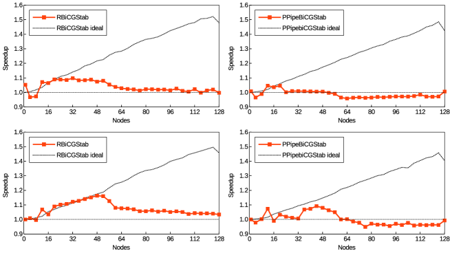
Figure 12: Simulation speedup due to manual progression of global non-blocking collective operations for preconditioners of different complexity. Top – $\alpha=20$; bottom – $\alpha=50$.

The increase in the preconditioner complexity (and in the number of MPI_Test calls) improves the communications overlap and allows to obtain the speedup for the Reordered BiCGStab of about 20%. Range of the nodes with ideal communications overlap is increased up to 48, and the 5% speedup is observed for the higher scales. The similar tendency is reproduced for the Pipelined BiCGStab method, but the peak speedup is limited by 10%, and the use of progression for more than 48 nodes still leads to a slowdown by 2-5%.

5 Conclusions

The efficiency of the classical BiCGStab iterative method and several modified formulations for solving systems of linear algebraic equations is investigated. The importance of reducing the costs of vector operations to achieve maximal performance is demonstrated. The vector merging technique is applied for the methods considered, and corresponding merged formulations of the methods allowing to minimize data transfers with the memory are proposed. While the merging of vector operations is applicable for all the methods, the effect is much more substantial for the modified formulations. The suggested optimization allows to reduce the extra vector operation costs and decrease the gap between the classical method and modified formulations. The observed speedup due to merging of vector operations is up to 30%.

The analytical execution time model is proposed to perform the detailed comparison of the methods. The model is based on the volume of data transfers with the memory. The accuracy of this model is demonstrated by the validation with the simulation results. The analytical model allows to predict the corresponding execution times with about 10% error.

The proposed analytical model is used for the detailed comparison of six iterative methods. The influence of the problem size, preconditioner complexity, number of RHS vectors, and the effect of global communications overlap on the choice of the optimal method are highlighted. It is shown that the modified methods can outperform the classical BiCGStab method when the global reduction time becomes comparable with the vector update time. The increase in the preconditioner complexity and the number of RHS vectors extends the range of optimality for the classical BiCGStab methods towards the higher scales in compute nodes. The corresponding theoretical predictions are validated by the numerical simulations, and the simulation results completely reproduce the predicted behaviour.

The progression of non-blocking global communications is among the key features required by the modified BiCGStab methods. In practice, however, the efficient asynchronous progression for the global reductions with short messages (8–8192 bytes) is a challenging issue. The manual progression is investigated and implemented in the corresponding test code. The performed experiments have shown that the manual progression can generally produce the overlap of communications by computations and speedup the calculations, but is problematic to be implemented in the computational codes.

Appendix A Compute platforms

The results of numerical experiments discussed in the paper were performed on compute systems Lomonosov and Lomonosov-2 installed in the Research Computing Center of Lomonosov Moscow State University. The main parameters of the supercomputers are summarized in tab. 7. The table also contains the real memory bandwidth values, obtained with help of STREAM benchmark [33]. It should be noted the last level cache (LLC) bandwidth values demonstrate observable deviations from run to run, thus the presented results should be treated as some reference values only.

Table 7: The main characteristics of Lomonosov and Lomonosov-2 supercomputers.

Supercomputer	Lomonosov	Lomonosov-2
Processor model	Intel Xeon X5570	Intel Xeon E5-2697v3
Processors	2	1
Cores	4	14
Instruction set	SSE4.2	AVX2
LLC size, MB	8	35
RAM Bandwidth, GB/s	16	60
LLC Bandwidth, GB/s	46	288
Interconnect	Infiniband QDR	Infiniband FDR

Appendix B Merged formulations of BiCGStab methods

The current section presents merged formulations of the modified BiCGStab methods discussed in the paper. The operations specified in the single line are performed in the merged form, i.e. with single loop over the vectors.

Algorithm 1 The BiCGStab method [2]

1:  $x_{0}$ = initial guess; $r_{0}=b-Ax_{0}$

2:  $\rho_{0}=(r_{0},r_{0})$

3:  $p_{0}=r_{0}$

4:  for $j=0,1,\ldots$ do

5:     $v_{j}=Ap_{j}$

6:     $\delta_{j}=(v_{j},r_{0})$

7:     $\alpha_{j}=\frac{\rho_{j}}{\delta_{j}}$

8:     $s_{j}=r_{j}-{\alpha_{j}}v_{j}$

9:     $t_{j}=As_{j}$

10:     $\phi_{j}=(t_{j},s_{j})$

11:     $\psi_{j}={(t_{j},t_{j})}$

12:     $\omega_{j}=\frac{\phi_{j}}{\psi_{j}}$

13:     $x_{j+1}=x_{j}+\alpha_{j}p_{j}+{\omega_{j}}s_{j}$

14:     $r_{j+1}=s_{j}-{\omega_{j}}t_{j}$

15:     if $(r_{j+1},r_{j+1})<\varepsilon^{2}$ then

16:        break

17:     end if

18:     $\rho_{j+1}=(r_{j+1},r_{0})$

19:     $\beta_{j}={\frac{\rho_{j+1}}{\rho_{j}}}{\frac{\alpha_{j}}{\omega_{j}}}$

20:     $p_{j+1}=r_{j+1}+{\beta_{j}}(p_{j}-{\omega_{j}}v_{j})$

21:  end for

Algorithm 2 The merged BiCGStab method

1:  $x_{0}$ = initial guess; $z=Ax_{0}$

2:  $r_{0}=b-z$, $\rho_{0}=(r_{0},r_{0})$, $p_{0}=r_{0}$

3:  for $j=0,1,\ldots$ do

4:     $v_{j}=Ap_{j}$

5:     $\delta_{j}=(v_{j},r_{0})$

6:     $\alpha_{j}=\frac{\rho_{j}}{\delta_{j}}$

7:     $s_{j}=r_{j}-{\alpha_{j}}v_{j}$

8:     $t_{j}=As_{j}$

9:     $\phi_{j}=(t_{j},s_{j})$, $\psi_{j}=(t_{j},t_{j})$, $\theta_{j}=(s_{j},s_{j})$

10:     $\omega_{j}=\frac{\phi_{j}}{\psi_{j}}$

11:     if $(\theta_{j}-\omega_{j}\phi_{j})<\varepsilon^{2}$ then

12:        $x_{j+1}=x_{j}+\alpha_{j}p_{j}+{\omega_{j}}s_{j}$,$r_{j+1}=s_{j}-{\omega_{j}}t_{j}$

13:        break

14:     end if

15:     $x_{j+1}=x_{j}+\alpha_{j}p_{j}+{\omega_{j}}s_{j}$, $r_{j+1}=s_{j}-{\omega_{j}}t_{j}$, $\rho_{j+1}=(r_{j+1},r_{0})$

16:     $\beta_{j}={\frac{\rho_{j+1}}{\rho_{j}}}{\frac{\alpha_{j}}{\omega_{j}}}$

17:     $p_{j+1}=r_{j+1}+{\beta_{j}}(p_{j}-{\omega_{j}}v_{j})$

18:  end for

Algorithm 3 The merged Improved BiCGStab method ⁴

1:  $x_{0}$ = initial guess; $r_{0}=b-Ax_{0}$, $u_{0}=Ar_{0}$, $f_{0}=A^{T}r_{0}$, $q_{0}=v_{0}=z_{0}=0$

2:  $\sigma_{-1}=\pi_{0}=\tau_{0}=0$, $\sigma_{0}=(r_{0},u_{0})$, $\rho_{0}=\alpha_{0}=\omega_{0}=1$, $\phi_{0}=(r_{0},r_{0})$

3:  for $j=0,1,\ldots$ do

4:     $\rho_{j+1}=\phi_{j}-\omega_{j}\sigma_{j-1}+\omega_{j}\alpha_{j}\pi_{j}$

5:     $\delta_{j+1}=\frac{\rho_{j+1}}{\rho_{j}}\alpha_{j}$, $\beta_{j+1}=\frac{\delta_{j+1}}{\omega_{j}}$

6:     $\tau_{j+1}=\sigma_{j}+\beta_{j+1}\tau_{j}-\delta_{j+1}\pi_{j}$

7:     $\alpha_{j+1}=\frac{\rho_{j+1}}{\tau_{j+1}}$

8:     $z_{j+1}=\alpha_{j+1}r_{j}+\beta_{j+1}\frac{\alpha_{j+1}}{\alpha_{j}}z_{j}-\alpha_{j+1}\delta_{j+1}v_{j}$, $v_{j+1}=u_{j}+\beta_{j+1}v_{j}-\delta_{j+1}q_{j}$, $s_{j+1}=r_{j}-\alpha_{j+1}v_{j+1}$

9:     $q_{j+1}=Av_{j+1}$

10:     $t_{j+1}=u_{j}-\alpha_{j+1}q_{j+1}$, $\phi_{j+1}=(r_{0},s_{j+1})$, $\pi_{j+1}=(r_{0},q_{j+1})$, $\gamma_{j+1}=(f_{0},s_{j+1})$, $\eta_{j+1}=(f_{0},t_{j+1})$, $\theta_{j+1}=(s_{j+1},t_{j+1})$, $\kappa_{j+1}=(t_{j+1},t_{j+1})$, $\nu_{j+1}=(s_{j+1},s_{j+1})$

11:     $\omega_{j+1}=\frac{\theta_{j+1}}{\kappa_{j+1}}$

12:     $\sigma_{j+1}=\gamma_{j+1}-\omega_{j+1}\eta_{j+1}$

13:     $r_{j+1}=s_{j+1}-\omega_{j+1}t_{j+1}$, $x_{j+1}=x_{j}+z_{j+1}+\omega_{j+1}s_{j+1}$

14:     if ($\nu_{j+1}-\omega_{j+1}\theta_{j+1})<\varepsilon^{2}$ then

15:        break

16:     end if

17:     $u_{j+1}=Ar_{j+1}$

18:  end for

Algorithm 4 The merged Pipelined BiCGStab method

1:  $x_{0}$ = initial guess; $r_{0}=b-Ax_{0}$, $w_{0}=Ar_{0}$, $t_{0}=Aw_{0}$

2:  $\rho_{0}=(r_{0},r_{0})$, $\alpha_{0}=\rho_{0}/(r_{0},w_{0})$, $\beta_{-1}=0$

3:  for $j=0,1,\ldots$ do

4:     $p_{j}=r_{j}+\beta_{j-1}(p_{j-1}-\omega_{j-1}s_{j-1})$, $s_{j}=w_{j}+\beta_{j-1}(s_{j-1}-\omega_{j-1}z_{j-1})$, $z_{j}=t_{j}+\beta_{j-1}(z_{j-1}-\omega_{j-1}v_{j-1})$, $q_{j}=r_{j}-\alpha_{j}s_{j}$, $y_{j}=w_{j}-\alpha_{j}z_{j}$, $\theta_{j}=(q_{j},y_{j})$, $\phi_{j}=(y_{j},y_{j})$, $\pi_{j}=(q_{j},q_{j})$

5:     $v_{j}=Az_{j}$

6:     $\omega_{j}=\frac{\theta_{j}}{\phi_{j}}$

7:     $x_{j+1}=x_{j}+\alpha_{j}p_{j}+\omega_{j}q_{j}$, $r_{j+1}=q_{j}-\omega_{j}y_{j}$

8:     if $(\pi_{j}-\omega_{j}\theta_{j})<\varepsilon^{2}$ then

9:        break

10:     end if

11:     $w_{j+1}=y_{j}-\omega_{j}(t_{j}-\alpha_{j}v_{j})$ $\rho_{j+1}=(r_{0},r_{j+1})$, $\psi_{j}=(r_{0},z_{j})$, $\sigma_{j}=(r_{0},w_{j+1})$, $\delta_{j}=(r_{0},s_{j})$

12:     $t_{j+1}=Aw_{j+1}$

13:     $\beta_{j}=(\alpha_{j}/\omega_{j})(\rho_{j+1}/\rho_{j})$

14:     $\alpha_{j+1}=\rho_{j+1}/(\sigma_{j}+\beta_{j}\delta_{j}-\beta_{j}\omega_{j}\psi_{j})$

15:  end for

Algorithm 5 The merged preconditioned BiCGStab method

1:  $x_{0}$ = initial guess; $r_{0}=b-Ax_{0}$

2:  $\rho_{0}=(r_{0},r_{0})$

3:  $p_{0}=r_{0}$

4:  for $j=0,1,\ldots$ do

5:     $\hat{p}_{j}=M^{-1}p_{j}$, $v_{j}=A\hat{p}_{j}$

6:     $\delta_{j}=(v_{j},r_{0})$

7:     $\alpha_{j}=\frac{\rho_{j}}{\delta_{j}}$

8:     $s_{j}=r_{j}-{\alpha_{j}}v_{j}$

9:     $\hat{s}_{j}=M^{-1}s_{j}$, $t_{j}=A\hat{s}_{j}$

10:     $\phi_{j}=(t_{j},s_{j})$, $\psi_{j}=(t_{j},t_{j})$, $\theta_{j}=(s_{j},s_{j})$

11:     $\omega_{j}=\frac{\phi_{j}}{\psi_{j}}$

12:     if $(\theta_{j}-\omega_{j}\phi_{j})<\varepsilon^{2}$ then

13:        $x_{j+1}=x_{j}+\alpha_{j}\hat{p}_{j}+{\omega_{j}}\hat{s}_{j}$

14:        $r_{j+1}=s_{j}-{\omega_{j}}t_{j}$

15:        break

16:     end if

17:     $r_{j+1}=s_{j}-{\omega_{j}}t_{j}$, $\rho_{j+1}=(r_{j+1},r_{0})$

18:     $\beta_{j}={\frac{\rho_{j+1}}{\rho_{j}}}{\frac{\alpha_{j}}{\omega_{j}}}$

19:     $x_{j+1}=x_{j}+\alpha_{j}\hat{p}_{j}+{\omega_{j}}\hat{s}_{j}$

20:     $p_{j+1}=r_{j+1}+{\beta_{j}}(p_{j}-{\omega_{j}}v_{j})$

21:  end for

Algorithm 6 The merged Reordered BiCGStab method ⁵

1:  $x_{0}$ = initial guess; $r_{0}=b-Ax_{0}$

2:  $\rho_{0}=(r_{0},r_{0})$

3:  $z_{0}=M^{-1}r_{0}$

4:  $\hat{v}_{0}=z_{0}$

5:  for $j=0,1,\ldots$ do

6:     $v_{j}=A\hat{v}_{j}$

7:     $\delta_{j}=(v_{j},r_{0})$

8:     $s_{j}=M^{-1}v_{j}$

9:     $\alpha_{j}=\frac{\rho_{j}}{\delta_{j}}$

10:     $\hat{t}_{j}=z_{j}-\alpha_{j}s_{j}$

11:     $t_{j}=A\hat{t}_{j}$

12:     $\tilde{r}_{j}=r_{j}-\alpha_{j}v_{j}$, $\theta_{j}=(t_{j},\tilde{r}_{j})$, $\phi_{j}=(t_{j},t_{j})$, $\psi_{j}=(t_{j},r_{0})$, $\eta_{j}=(\tilde{r}_{j},\tilde{r}_{j})$

13:     $q_{j}=M^{-1}t_{j}$

14:     $\omega_{j}=\frac{\theta_{j}}{\phi_{j}}$

15:     $r_{j+1}=\tilde{r}_{j}-\omega_{j}t_{j}$

16:     if $(\eta_{j}-\omega_{j}\theta_{j})<\varepsilon^{2}$ then

17:        $x_{j+1}=x_{j}+\alpha_{j}\hat{v}_{j}+\omega_{j}\hat{t}_{j}$

18:        break

19:     end if

20:     $\rho_{j+1}=-\omega_{j}\psi_{j}$

21:     $\beta_{j}={\frac{\rho_{j+1}}{\rho_{j}}}{\frac{\alpha_{j}}{\omega_{j}}}$

22:     $x_{j+1}=x_{j}+\alpha_{j}\hat{v}_{j}+\omega_{j}\hat{t}_{j}$, $z_{j+1}=\hat{t}_{j}-\omega_{j}q_{j}$, $\hat{v}_{j+1}=z_{j+1}+\beta_{j}(\hat{v}_{j}-\omega_{j}s_{j})$

23:  end for

Algorithm 7 The merged preconditioned Pipelined BiCGStab method

1:  $x_{0}$ = initial guess; $r_{0}=b-Ax_{0}$, $\hat{r}_{0}=M^{-1}r_{0}$, $w_{0}=A\hat{r}_{0}$, $\hat{w}_{0}=M^{-1}\hat{w}_{0}$, $t_{0}=A\hat{w}_{0}$

2:  $\rho_{0}=(r_{0},r_{0})$, $\alpha_{0}=\rho_{0}/(r_{0},w_{0})$, $\beta_{-1}=0$

3:  for $j=0,1,\ldots$ do

4:     $\hat{p}_{j}=\hat{r}_{j}+\beta_{j-1}(\hat{p}_{j-1}-\omega_{j-1}\hat{s}_{j-1})$, $\hat{s}_{j}=\hat{w}_{j}+\beta_{j-1}(\hat{s}_{j-1}-\omega_{j-1}\hat{z}_{j-1})$, $\hat{q}_{j}=\hat{r}_{j}-\alpha_{j}\hat{s}_{j}$

5:     $s_{j}=w_{j}+\beta_{j-1}(s_{j-1}-\omega_{j-1}z_{j-1})$, $z_{j}=t_{j}+\beta_{j-1}(z_{j-1}-\omega_{j-1}v_{j-1})$, $q_{j}=r_{j}-\alpha_{j}s_{j}$, $y_{j}=w_{j}-\alpha_{j}z_{j}$, $\theta_{j}=(q_{j},y_{j})$, $\phi_{j}=(y_{j},y_{j})$, $\pi_{j}=(q_{j},q_{j})$

6:     $\hat{z}_{j}=M^{-1}z_{j}$, $v_{j}=A\hat{z}_{j}$

7:     $\omega_{j}=\frac{\theta_{j}}{\phi_{j}}$

8:     if $(\pi_{j}-\omega_{j}\theta_{j})<\varepsilon^{2}$ then

9:        $x_{j+1}=x_{j}+\alpha_{j}\hat{p}_{j}+\omega_{j}\hat{q}_{j}$

10:        $r_{j+1}=q_{j}-\omega_{j}y_{j}$

11:        break

12:     end if

13:     $x_{j+1}=x_{j}+\alpha_{j}\hat{p}_{j}+\omega_{j}\hat{q}_{j}$, $\hat{r}_{j+1}=\hat{q}_{j}-\omega_{j}(\hat{w}_{j}-\alpha_{j}\hat{z}_{j})$

14:     $r_{j+1}=q_{j}-\omega_{j}y_{j}$, $w_{j+1}=y_{j}-\omega_{j}(t_{j}-\alpha_{j}v_{j})$, $\rho_{j+1}=(r_{0},r_{j+1})$, $\psi_{j}=(r_{0},z_{j})$, $\sigma_{j}=(r_{0},w_{j+1})$, $\delta_{j}=(r_{0},s_{j})$

15:     $\hat{w}_{j}=M^{-1}w_{j}$, $t_{j}=A\hat{w}_{j}$

16:     $\beta_{j}=(\alpha_{j}/\omega_{j})(\rho_{j+1}/\rho_{j})$

17:     $\alpha_{j+1}=\rho_{j+1}/(\sigma_{j}+\beta_{j}\delta_{j}-\beta_{j}\omega_{j}\psi_{j})$

18:  end for

Appendix C Benchmarking efficiency of asynchronous non-blocking Allreduce operations

The efficiency of the asynchronous progression of global communications is among the key factors influencing on the choice of the optimal iterative method. The test platform used in the present paper for parallel simulations has InfiniBand interconnect and does not provide hardware-based progression for asynchronous execution of non-blocking global communications, thus focusing the interest on two other progression techniques. The efficiency of the non-blocking global communications can be measured with help of Intel MPI benchmark [23], and specifically the IMB-NBC collection of benchmarks [35]. These benchmarks allow to compare the execution times for blocking and non-blocking operations, and estimate the communication/computation overlap. The basic functionality, however, does not allow to measure the efficiency of manual progression. To cover all the simulation scenarios of interest the modified benchmark has been developed. The proposed benchmark measures three simulation scenarios: blocking global reduction followed by the computations, non-blocking global reduction overlapped by the computations, and non-blocking global reduction overlapped by the computations with manual progression. The corresponding simulation scenarios are summarized in Figure 13. The calculations are performed in the form of vector updates, and the size of the vectors is chosen in order to balance the computations with communications. The number of loop iterations, $N_{it}$, in the experiments varies from 10 to 100 to estimate the typical number of $MPI\_Test$ calls needed to progress the global communication as a function of the number of computational processes. The overall amount of computations is preserved constant by changing the vector size. The experiments are performed up to 192 compute nodes with 8 MPI processes per each node.

⬇

// mode #1:

MPI_Allreduce(...);

for (i = 0; i < N_it; i++)

vector_op(...);

// mode #2:

MPI_Iallreduce(..., &req);

for (i = 0; i < N_it; i++)

vector_op(...);

MPI_Wait(&req, ...);

// mode #3:

MPI_Iallreduce(..., &req);

for (i = 0; i < N_it; i++) {

vector_op(...);

MPI_Test(&req, ...);

}

MPI_Wait(&req, ...);

Figure 13: Execution scenarios performed in the asynchronous non-blocking Allreduce communications benchmark.

The corresponding tests performed on Lomonosov supercomputer with Intel MPI library 2017 demonstrate that the basic implementation of asynchronous data transfer without additional progression (mode #2) does not allow to obtain any observable performance gain compared the synchronous operation (mode #1). The execution time for MPI_Iallreduce function is much lower compared the blocking one, but the total time of MPI_Iallreduce and MPI_Wait functions is about the same as for MPI_Allreduce function (Figure 14). Despite the significant time spent on computations, which theoretically can hide the latency of global communications, in practice the progress is not automatically performed.

The third execution scenario investigates the effect of MPI_Test function calls to handle the message progression. While the systematic MPI_Test calls affect the efficiency of the computations, the manual progression allows to obtain overlapping of communications and computations. The corresponding overlapping overhead is estimated by the following parameter

$$\gamma^{i}=\frac{T_{calc}^{\#i}+T_{comm}^{\#i}-T_{calc}^{\#1}}{T_{comm}^{\#1}},$$ (24)

characterizing ratio of the non-blocking communication time to the blocking one, and also accounting increase in the calculation time. Results presented in Figure 14 demonstrate that manual progression allows to reduce the global communications time. Starting from 16 nodes the corresponding communications time can be reduced at least twofold.

The influence of the number of MPI_Test calls on the efficiency of message progression is shown in Figure 15. For the short messages the optimal number of internal loop iterations is close to 10. The increase in the number of iterations decreases the time spent on final MPI_Wait function call, but increases the time spent on multiple MPI_Test calls. The optimal number of iterations grows with the message size: for the messages of 2048 bytes the corresponding value increases to 20–30 iterations with overall improvement in the efficiency of communications overlap.

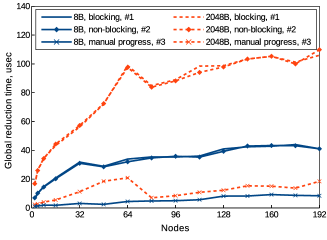
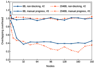
Figure 14: Execution times and overlapping overhead for global reduction operations with different execution scenarios. Left – cumulative times for data transfer functions (MPI_Allreduce/MPI_Iallreduce and MPI_Wait); right – overlapping overhead, $N_{it}=20$.

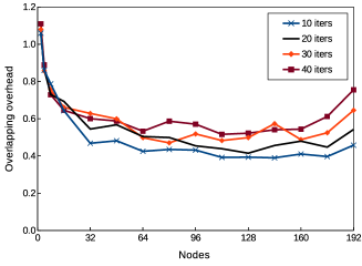
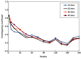
Figure 15: Influence of the number of MPI_Test calls on overlapping overhead. Left – message size 8 bytes; right – message size 2048 bytes.

Intel MPI library 2017 used in the presented calculations provides software progression functionality, which can be enabled by setting the environment variable I_MPI_ASYNC_PROGRESS = 1. Activating this option, the library creates progression threads to handle the asynchronous non-blocking message progression. The corresponding functionality has been investigated using the same benchmark described above. Comparison of the obtained results shows that software progression leads to a significant slowdown of both communications and computations: the latency of blocking reduction operation increases by a factor of 40. This observation also correlates with the obtained IMB-NBC Iallreduce benchmark results and [23]. Despite the almost ideal overlap of communications and computations, the overall time of global reduction and computations becomes more than by an order of magnitude higher compared the one without software progression (Figure 16). Reducing the number of MPI processes per node and changing the threads pinning rule does not allow to obtain any observable improvement in the communication time. This fact makes the corresponding functionality inapplicable for the computational algorithms massively performing global reductions with small vectors.

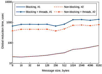
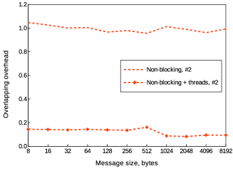
Figure 16: Execution times and overlapping overhead for global reductions with asynchronous progression threads. Left – cumulative times for data transfer functions (MPI_Allreduce/MPI_Iallreduce and MPI_Wait); right – overlapping overhead.

References

- [1] M. R. Hestenes, E. Stiefel, Methods of conjugate gradients for solving linear systems, Journal of Research of the National Bureau of Standards 49 (6) (1952) 409–436.
- [2] H. A. van der Vorst, BI-CGSTAB: a fast and smoothly converging variant of BI-CG for the solution of nonsymmetric linear systems, SIAM J. Sci. Stat. Comput. 13 (2) (1992) 631–644. doi:10.1137/0913035.
- [3] Y. Saad, M. H. Schultz, GMRES: a generalized minimal residual algorithm for solving nonsymmetric linear systems, SIAM J. Sci. Stat. Comput. 7 (3) (1986) 856–869. doi:10.1137/0907058.
- [4] T. Jacques, L. Nicolas, C. Vollaire, Electromagnetic scattering with the boundary integral method on MIMD systems, in: High-Performance Computing and Networking, Vol. 1593 of Lecture Notes in Computer Science, Springer Berlin / Heidelberg, 1999, pp. 1025–1031. doi:10.1007/BFb0100663.
- [5] L. Yang, R. Brent, The improved BiCGStab method for large and sparse unsymmetric linear systems on parallel distributed memory architectures, in: Fifth International Conference on Algorithms and Architectures for Parallel Processing (ICA3PP’02). Proceedings., IEEE Computer Society, Los Alamitos, CA, USA, 2002, pp. 324–328. doi:10.1109/ICAPP.2002.1173595.
- [6] B. Krasnopolsky, The reordered BiCGStab method for distributed memory computer systems, Procedia Computer Science 1 (1) (2010) 213–218, ICCS 2010. doi:10.1016/j.procs.2010.04.024.
- [7] S. Cools, W. Vanroose, The communication-hiding pipelined BiCGstab method for the parallel solution of large unsymmetric linear systems, Parallel Computing 65 (2017) 1–20. doi:10.1016/j.parco.2017.04.005.
- [8] E. Carson, N. Knight, J. Demmel, Avoiding communication in nonsymmetric Lanczos-based Krylov subspace methods, SIAM Journal on Scientific Computing 35 (5) (2013) S42–S61. doi:10.1137/120881191.
-
[9]
M. Naumov,
S-step
and communication-avoiding iterative methods, Tech. Rep. NVR-2016-003
(2016).
URL https://research.nvidia.com/sites/default/files/pubs/2016-04_S-Step-and-Communication-Avoiding/nvr-2016-003.pdf - [10] J. I. Aliaga, J. Pérez, E. S. Quintana-Ortí, H. Anzt, Reformulated conjugate gradient for the energy-aware solution of linear systems on GPUs, in: Proceedings of the International Conference on Parallel Processing, 2013, pp. 320–329. doi:10.1109/ICPP.2013.41.
- [11] H. Anzt, S. Tomov, P. Luszczek, W. Sawyer, J. Dongarra, Acceleration of GPU-based Krylov solvers via data transfer reduction, The International Journal of High Performance Computing Applications 29 (3) (2015) 366–383. doi:10.1177/1094342015580139.
- [12] J. I. Aliaga, J. Pérez, E. S. Quintana-Ortí, Systematic fusion of CUDA kernels for iterative sparse linear system solvers, in: J. L. Träff, S. Hunold, F. Versaci (Eds.), Euro-Par 2015: Parallel Processing, Springer Berlin Heidelberg, Berlin, Heidelberg, 2015, pp. 675–686. doi:10.1007/978-3-662-48096-0_52.
- [13] K. Rupp, J. Weinbub, A. Jüngel, T. Grasser, Pipelined iterative solvers with kernel fusion for graphics processing units, ACM Trans. Math. Softw. 43 (2) (2016) 11:1–11:27. doi:10.1145/2907944.
- [14] S. Williams, A. Waterman, D. Patterson, Roofline: An insightful visual performance model for multicore architectures, Communications of the ACM 52 (4) (2009) 65–76. doi:10.1145/1498765.1498785.
-
[15]
Basic linear
algebra subprograms technical (BLAST) forum standard (Aug. 2001).
URL http://www.netlib.org/blas/blast-forum/blas-report.pdf -
[16]
HYPRE: High performance
preconditioners.
URL http://www.llnl.gov/CASC/hypre/ - [17] E. de Sturler, H. A. van der Vorst, Communication cost reduction for Krylov methods on parallel computers, in: W. Gentzsch, U. Harms (Eds.), High-Performance Computing and Networking, Springer Berlin Heidelberg, Berlin, Heidelberg, 1994, pp. 190–195. doi:10.1007/3-540-57981-8_115.
- [18] S.-X. Zhu, T.-X. Gu, X.-P. Liu, Minimizing synchronizations in sparse iterative solvers for distributed supercomputers, Computers & Mathematics with Applications 67 (1) (2014) 199–209. doi:10.1016/j.camwa.2013.11.008.
- [19] S. Zhang, GPBi-CG: Generalized product-type methods based on Bi-CG for solving nonsymmetric linear systems, SIAM Journal on Scientific Computing 18 (2) (1997) 537–551. doi:10.1137/S1064827592236313.
- [20] S. Fujino, GPBiCG(m,l): A hybrid of BiCGSTAB and GPBiCG methods with efficiency and robustness, Applied Numerical Mathematics 41 (1) (2002) 107–117, developments and Trends in Iterative Methods for Large Systems of Equations - in memorium Rudiger Weiss. doi:10.1016/S0168-9274(01)00113-1.
- [21] Y. Saad, Iterative methods for sparse linear systems, 2nd edition, SIAM, Philadelpha, PA, 2003.
- [22] B. Krasnopolsky, An approach for accelerating incompressible turbulent flow simulations based on simultaneous modelling of multiple ensembles, Computer Physics Communications 229 (2018) 8–19. doi:10.1016/j.cpc.2018.03.023.
-
[23]
Intel
MPI benchmark.
URL https://software.intel.com/en-us/articles/intel-mpi-benchmarks -
[24]
Message Passing Interface Forum,
MPI: A
Message-Passing Interface Standard, Version 3.1 (2015).
URL https://www.mpi-forum.org/docs/mpi-3.1/mpi31-report.pdf -
[25]
V. Cardellini, A. Fanfarillo, S. Filippone,
Overlapping
communication with computation in MPI applications, techreport, Universita
di Roma ”Tor Vergata” (2016).
URL https://art.torvergata.it/retrieve/handle/2108/140530/291158/mpiprog.pdf - [26] T. Hoefler, A. Lumsdaine, Message progression in parallel computing - to thread or not to thread?, in: Proc. of 2008 IEEE International Conference on Cluster Computing, 2008. doi:10.1109/clustr.2008.4663774.
- [27] M. Si, A. J. Peña, J. Hammond, P. Balaji, M. Takagi, Y. Ishikawa, Dynamic Adaptable Asynchronous Progress Model for MPI RMA Multiphase Applications, IEEE Transactions on Parallel and Distributed Systems 29 (9) (2018) 1975–1989. doi:10.1109/TPDS.2018.2815568.
- [28] A. Ruhela, H. Subramoni, S. Chakraborty, M. Bayatpour, P. Kousha, D. K. Panda, Efficient Asynchronous Communication Progress for MPI Without Dedicated Resources, in: Proceedings of the 25th European MPI Users’ Group Meeting, EuroMPI’18, ACM, New York, NY, USA, 2018, pp. 14:1–14:11. doi:10.1145/3236367.3236376.
- [29] A. Denis, J. Jaeger, H. Taboada, Progress Thread Placement for Overlapping MPI Non-blocking Collectives Using Simultaneous Multi-threading, in: G. Mencagli, D. B. Heras, V. Cardellini, E. Casalicchio, E. Jeannot, F. Wolf, A. Salis, C. Schifanella, R. R. Manumachu, L. Ricci, M. Beccuti, L. Antonelli, J. D. Garcia Sanchez, S. L. Scott (Eds.), Euro-Par 2018: Parallel Processing Workshops, Springer International Publishing, 2019, pp. 123–133. doi:10.1007/978-3-030-10549-5_10.
-
[30]
A. Medvedev,
Towards
benchmarking the asynchronous progress of non-blocking MPI point-to-point
and collective operations (2019).
URL https://github.com/a-v-medvedev/mpi-benchmarks/blob/master/doc/progression-article_v2.pdf - [31] C. Chevalier, F. Pellegrini, PT-Scotch: A tool for efficient parallel graph ordering, Parallel Computing 34 (6) (2008) 318–331, parallel Matrix Algorithms and Applications. doi:10.1016/j.parco.2007.12.001.
- [32] G. Karypis, K. Schloegel, Parallel Graph Partitioning and Sparse Matrix Ordering Library (2003).
- [33] J. D. McCalpin, Memory bandwidth and machine balance in current high performance computers, IEEE Computer Society Technical Committee on Computer Architecture (TCCA) Newsletter (1995) 19–25.
-
[34]
S. Balay, S. Abhyankar, M. F. Adams, J. Brown, P. Brune, K. Buschelman,
L. Dalcin, A. Dener, V. Eijkhout, W. D. Gropp, D. Kaushik, M. G. Knepley,
D. A. May, L. C. McInnes, R. T. Mills, T. Munson, K. Rupp, P. Sanan, B. F.
Smith, S. Zampini, H. Zhang, H. Zhang,
PETSc Web page,
http://www.mcs.anl.gov/petsc (2018).
URL http://www.mcs.anl.gov/petsc -
[35]
M. Brinskiy, A. Supalov, M. Chuvelev, E. Leksikov,
Mastering
performance challenges with the new MPI-3 standard, The Parallel Universe
18 (1) (2014) 33–40.
URL https://software.intel.com/sites/default/files/managed/6a/78/parallel_mag_issue18.pdf