Prudence When Assuming Normality:
an advice for machine learning practitioners

Abstract

In a binary classification problem the feature vector (predictor) is the input to a scoring function that produces a decision value (score), which is compared to a particular chosen threshold to provide a final class prediction (output). Although the normal assumption of the scoring function is important in many applications, sometimes it is severely violated even under the simple multinormal assumption of the feature vector. This article proves this result mathematically with a counter example to provide an advice for practitioners to avoid blind assumptions of normality. On the other hand, the article provides a set of experiments that illustrate some of the expected and well-behaved results of the Area Under the ROC curve (AUC) under the multinormal assumption of the feature vector. Therefore, the message of the article is not to avoid the normal assumption of either the input feature vector or the output scoring function; however, a prudence is needed when adopting either of both.

1 Introduction

1.1 Formalization and Notation

If a random vector $X$ and a random variable $Y$ have a joint probability density $f_{X,Y}(x,y)$, and $Y$ is qualitative (or categorical) with only two possible values (class $\omega_{1}$ or class $\omega_{2}$) the binary classification problem is defined as follows: how to find the classification rule $\hat{Y}=\eta(X)$ that is able to predict the class $Y$ (the response) from an observed value for the variable $X$ (the predictor). The prediction function is required to have minimum average prediction error, which is defined in terms of some loss function $L(Y,\eta(X))$ that penalizes for any deviation in the predicted value $\hat{Y}$ of the response from the correct value $Y$. Since $Y$ takes one of two values ($\omega_{1}$ or $\omega_{2}$), the loss function can be defined by the matrix $L(Y,\hat{Y})=((c_{ij})),\ i,j=1,2$, where the non-negative element $c_{ij}$ is the cost, the penalty or the price, paid for classifying an observation as $\omega_{j}$ when it belongs to $\omega_{i}$. Then, the risk of this prediction function is defined by the average loss, according to the defined loss function, which can be written as $R(\eta)=E\left[{L(Y,\hat{Y})}\right]$. These foundations can be found in, e.g., Hastie et al. (2009); Duda et al. (2001); Bishop (2006). It is known from the statistical decision theory that the rule $\eta$ that minimizes this risk $R$ is given by

$$\eta(x):\quad\frac{f_{X}(X=x|\omega_{1})}{f_{X}(X=x|\omega_{2})}\underset{\omega_{2}}{\overset{\omega_{1}}{\gtrless}}\frac{\Pr\left[\omega_{2}\right]\left({c_{22}-c_{21}}\right)}{\Pr\left[\omega_{1}\right]\left({c_{11}-c_{12}}\right)}.$$ (1)

However, in the feature subspace, $X\in\mathbf{R}^{p}$, the regions of classification (the solution to the inequality (1)) have the dimensionality $p$, and it is very difficult to calculate the error components from multi-dimensional integration. It is easier to look at (1) as:

$$\eta(x):\quad h(x)\underset{\omega_{2}}{\overset{\omega_{{}_{1}}}{\gtrless}}th,$$ (2a)

$$h(x)=\log\frac{f_{X}(X=x|\omega_{1})}{f_{X}(X=x|\omega_{2})},$$ (2b)

$$th=\log\frac{\Pr\left[\omega_{1}\right]\left({c_{22}-c_{21}}\right)}{\Pr\left[\omega_{2}\right](c_{11}-c_{12})},$$ (2c)

and $h(X)$ is called the log-likelihood ratio and acts as the decision value or the score. Now the log-likelihood ratio itself is a random variable whose variability comes from the feature vector $X$, and has a PDF conditional on the true class. This is shown in Figure 1. It can be easily shown that the two curves in Figure 1 cross at $h(X)=0$, when the threshold is zero ($th=0$).

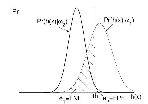
Figure 1: The probability of log-likelihood ratio conditional under each class. The two components of error are indicated as the FPF and FNF, the conventional terminology in medical imaging.

Now, if the joint distribution is known but its parameters are not known, a learning process is used to estimate those parameters from a training sample $\mathbf{t}$ by methods of statistical inference. Moreover, if the joint distribution is unknown, a classification function is modeled parametrically or nonparametrically and a training sample is used to build that model. This is the field of statistical learning, machine learning, or the recently so called “data science”. In either cases there is a modeled decision function (or scoring function) $h(X)$, that is no longer the log-likelihood ratio, and the final classification rule takes the form (2a). However, of course, it is no longer the optimal classification rule that minimizes the risk.

Regardless of how we obtain the decision (scoring) function $h(X)$, there should be some measure to assess the performance of the classification rule. Said differently, if several classifiers are competing in the same problem, which is better? One natural answer is to define the two types of error: $e_{1}$ is the probability of classifying a case as belonging to class 2 when it belongs to class 1, and $e_{2}$ is vice versa. Formally, this is defined as:

$$e_{1} =\int_{-\infty}^{th}{f_{h}}\left({h(x)|\omega_{1}}\right){dh(x)},$$ (3a)

$$e_{2} =\int_{th}^{\infty}{f_{h}}\left({h(x)|\omega_{2}}\right){dh(x)}$$ (3b)

It is conventional in some fields, e.g., medical imaging, to refer to $e_{1}$ as the False Negative Fraction (FNF), and $e_{2}$ as the False Positive Fraction (FPF). This is because diseased patients typically have a higher output value for a test than non-diseased patients. For example, a patient belonging to class 1 whose test output value is less than the threshold setting for the test will be called “test negative” while the patient is in fact in the diseased class. This is a false negative decision; hence the name FNF. The situation is reversed for the other error component. These components are illustrated in Figure 1.

Now assume the classifier is trained under the condition of equal prevalence and cost, i.e., $th=0$. In other environments there will be different a priori probabilities yielding to different threshold values. The error is not a sufficient measure now, since it is function of a single fixed threshold. A more general way to assess a classifier is provided by the Receiver Operating Characteristic (ROC) curve. This is a plot for the two components of error, $e_{1}$ and $e_{2}$ under different threshold values. However, a convention in several fields, e.g., medical imaging, is to plot the $TPF=1-FNF$ vs. the $FPF$.

Since the error components (3) are integrals over a particular PDF, the resulting ROC is a monotonically non-decreasing function. In that case, the farther apart the two distributions of the score function from each other, the higher the ROC curve and the larger the area under the curve (AUC). Figure 2 shows ROC curves for two different classifiers.

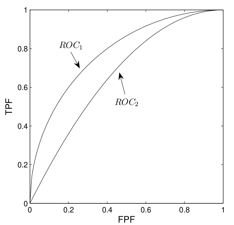
Figure 2: ROC curves for two different classifiers. ROC₁ is better than ROC₂, since for any error component value, the other component of classifier 1 is less than that one of classifier 2.

The first one performs better since it has a lower value of $e_{2}$ at each value of $e_{1}$. Thus, the first classifier unambiguously separates the two classes better than the second one. Also, the AUC for the first classifier is larger than that for the second one. AUC can be thought of as one summary measure for the ROC curve. Formally the AUC is given by:

$$AUC=\int_{0}^{1}{TPF\leavevmode\nobreak\ d(FPF)}$$ (4)

If two ROC curves cross, this means each is better than the other for a certain range of the threshold setting, but it is worse in another range. In that case some other measure can be used, such as the partial area under the curve (PAUC) in a specified region, which is quite out of the scope of the present article, e.g., see Jiang et al. (1996); Walter (2005); Yousef (2013). It is easy to show that the AUC defined in (4) is equivalent to:

$$AUC =\Pr\left[h\left({x|\omega_{2}}\right)<h\left({x|\omega_{1}}\right)\right],$$ (5)

which expresses again the separation between the two sets of decision scores $h(X|\omega_{1})$ and $h(X|\omega_{2})$.

The expressions (3), (4), and (5) are population parameters that are calculated from integrals assuming the full knowledge of distributions. However, in practical setups only a finite testing dataset is available and only estimates of these values are available. The Uniform Minimum Variance Unbiased Estimators (UMVUE) under the nonparametric assumptions are given by (Randles and Wolfe, 1979; Hájek et al., 1999):

$$\hat{e}_{1} =\sum\limits_{i=1}^{n_{1}}I_{h(x_{i}|\omega_{1})<th}$$ (6a)

$$\hat{e}_{2} =\sum\limits_{j=1}^{n_{2}}I_{h(x_{j}|\omega_{2})>th}$$ (6b)

$$\widehat{AUC} =\frac{1}{n_{1}n_{2}}\sum\limits_{j=1}^{n_{2}}{\sum\limits_{i=1}^{n_{1}}{\psi\left({h\left({x_{i}|\omega_{1}}\right),h\left({x_{j}|\omega_{2}}\right)}\right)}},$$ (6c)

$$\psi(a,b) =\left\{\begin{array}[c]{ccc}1&&a>b\\ 1/2&&a=b\\ 0&&a<b\end{array}\right.$$ (6g)

It is worth mentioning that, for a particular classification rule trained on the training data set $\mathbf{t}$, the expressions (3), (4), and (5) and their estimates (6) all should be subscripted by $\mathbf{t}$ since everything will vary with varying $\mathbf{t}$. We usually drop the subscript when there is no ambiguity.

1.2 Background and Motivation

From the introduction above, it is clear that a classifier trained on the training set $\mathbf{t}$ produces a decision (scoring) function $h_{\mathbf{t}}(X)$ that has its own distribution under each class. This distribution determines the errors, ROC, AUC, and any other performance measure. It is always tempting to assume normality for a random variable for easier mathematical analysis or statistical inference. For binary classification problem, in particular, normality can be assumed for either the final scoring function and/or the input feature vector. This will be elaborated next in the following two paragraphs.

First, the normality assumption of the two distributions of the scoring function $h(X)$ (under the two classes) is known as binormal model and has very interesting properties. These properties, along with their proofs exist in many texts and articles including very early literature, e.g., Green and Swets (1966); Dorfman et al. (1992); Pan and Metz (1997); Metz and Pan (1999); Dorfman et al. (1997); Krzanowski and Hand (2009). Under this assumption, the errors (3) clearly are given by a simple integration over the tail of normal distributions; and interestingly, the ROC curve is expressed using the inverse error function transformation, as:

$$\phi^{-1}(TPF)=\frac{(\mu_{1}-\mu_{2})}{\sigma_{1}}+(\frac{\sigma_{2}}{\sigma_{1}})\phi^{-1}(FPF).$$ (7)

This means that the whole ROC curve can be summarized in just two parameters: the intercept, and the slope; this is shown in Figure 3. Denote the intercept and slope of (7) by $a$ and $b$ respectively; it is easy to show that the AUC (4) will then be given by

$$AUC=\phi\left(\frac{a}{1+b^{2}}\right).$$ (8)

Figure 3: The double-normal-deviate plot for the ROC under the normal assumption for the log-likelihood ratio is a straight line.

Second, the normality assumption of the two distributions of the feature vector $X$ (the predictor) has another set of interesting results and properties of the performance measures as well. E.g., the early analysis by Fukunaga, in both mean and variance as a function of the training set size, is fundamental (Fukunaga, 1990; Fukunaga and Hayes, 1989a, b).

After the introduction above, it is very important to emphasize that it is not the intention of the present article to discourage any practitioner from using the normal assumption for either the feature vector or the scoring function. However, the objective is to illustrate how care and prudence are needed when assuming normality as it may be violated severely even in very simple setups, which may be counter-intuitive. The roadmap of the manuscript goes as follows.

1.3 Manuscripat Roadmap

Section 2 analyzes and derives mathematically, under the multinormal assumption of the feature vector $X$, how the scoring function can be a single-tailed or exponential-like distribution, which is a very sever violation from the binormal model. Section 3 complements the article and provides some expected and intuitive experimental results of the AUC under the multinormal assumption of the feature vector $X$. This emphasizes the objective of the article that we do not discourage from using the normal assumption; however, we urge practitioners for prudence towards adopting the assumption. Section 4 concludes the article.

2 Distribution of Log-Likelihood Under Multinormal Assumption: a counter-intuitive example

It may be instructive to examine, analytically, what the log-likelihood ratio looks under the popular data population of the feature vector:s the multinormal distribution. Consider two different classes, $\omega_{1}$and $\omega_{2}$, whose $p$-dimensional feature vectors have the multinormal distributions $F_{1}$ and $F_{2}$ respectively, described by the PDFs:

$$f_{X}(x|\omega_{i})=\frac{1}{(2\pi)^{p/2}\left|{\Sigma_{i}}\right|^{1/2}}\exp\left[{-\frac{1}{2}(x-\mu_{i}{)}^{\prime}\Sigma_{i}^{-1}(x-\mu_{i})}\right],\leavevmode\nobreak\ i=1,2$$ (9)

The Bayes classifier is the optimal one; it has the minimum risk (see Section 1). The training for the Bayes classifier in the multinormal case requires only the estimation of the mean vectors $\mu_{i}$ and the covariance matrices $\Sigma_{i}$. Assume that the training set for $\omega_{1}$ is $\mathbf{t}_{1}=\{t_{i}:t_{i}=(x_{i},\omega_{1})\},\leavevmode\nobreak\ i=1,\ldots,n_{1}$, and the training set for $\omega_{2}$ is $\mathbf{t}_{2}=\{t_{i}:t_{i}=(x_{i},\omega_{2})\},\leavevmode\nobreak\ i=1,\ldots,n_{2}$. The estimates of the population parameters are given by (Anderson, 2003):

$$\hat{\Sigma}_{i} =\frac{1}{n_{i}-1}\left[{\sum\limits_{j=1}^{n_{i}}{(x_{j}-\hat{\mu}_{i})(x_{j}-\hat{\mu}_{i}{)}^{\prime}}}\right],$$ (10)

$$\hat{\mu}_{i} =\frac{1}{n_{i}}\sum\limits_{j=1}^{n_{i}}{x_{j}},\leavevmode\nobreak\ x_{j}\in\omega_{i}$$ (11)

The log-likelihood function (2b), in combination with the estimated parameters (10) and (11), assuming equal prevalence for the two classes and equal costs for the two kinds of errors, can be written as:

$$h(X)=-\frac{1}{2}\left[{(X-\hat{\mu}_{1}{)}^{\prime}\hat{\Sigma}_{1}^{-1}(X-\hat{\mu}_{1})-(X-\hat{\mu}_{2}{)}^{\prime}\hat{\Sigma}_{2}^{-1}(X-\hat{\mu}_{2})}\right]-\frac{1}{2}\ln\frac{\left|{\hat{\Sigma}_{1}}\right|}{\left|{\hat{\Sigma}_{2}}\right|}$$ (12)

It should be noted that if the a priori probabilities and costs, which form a particular threshold value of the testing environment, are known they should be included in the log-likelihood ratio. I.e., the log of the R.H.S. of inequality (1) should be added to the R.H.S. of (12). In that case, the classifier is designed to be used in this environment having that threshold. For demonstration, consider the population parameters to take the following values:

$$\mu_{1}=\begin{pmatrix}2\\ 2\end{pmatrix},\quad\Sigma_{1}=\begin{pmatrix}1&.2\\ .2&1\end{pmatrix},\quad\mu_{2}=\begin{pmatrix}1\\ 1\end{pmatrix},\quad\Sigma_{2}=\begin{pmatrix}.3&.1\\ .1&.3\end{pmatrix}.$$ (13)

Consider that we train on a very large size of observations such that the estimated parameters are almost the same as the true ones. Under these parameters the two PDFs (9) of the two classes are shown in Figure 4 (left). Two simulated data sets, one set for each class with $10,000$ observations per class, are simulated from binormal distributions with the above parameters and illustrated in Figure 4 (right).

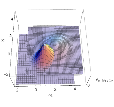
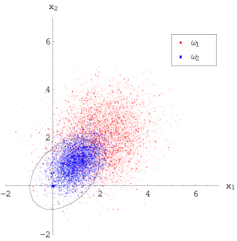
Figure 4: Two Binormal distributions. Left: a 3-D illustration of their Probability Density Function (PDF). Right: two simulated data sets from the two distributions, where the number of observations per class is $10,000$.

Under these parameter values, the log-likelihood ratio in (12), along with its contour plot is plotted in Figure 5. The locus separating the two classes in Figure 4 is obtained by solving $h(X)=0$ in (12).

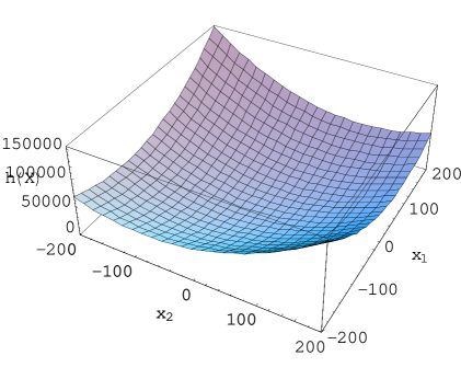
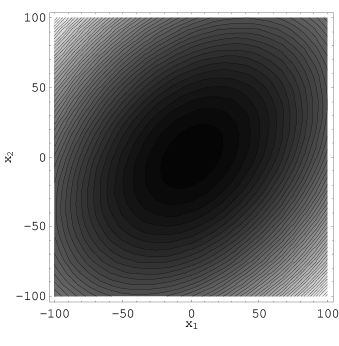
Figure 5: The log-likelihood ratio function of two features $x_{1}$ and $x_{2}$. Left: a 3-D representation. Right: its contour plot.

We next find the probability distributions of $h(X)$ in (12), under the two classes, which is a function of the random vector $X=(x_{1},x_{2})^{\prime}$. Consider the transformation $T:X\longrightarrow(h,d)$, where $d$ is a dummy variable set as

$$d=x_{1}$$ (14)

The dummy variable here is introduced just for clarity and we could have written $T:X\longrightarrow(h,x_{1})$. We shall, no longer, refer to $d$; rather, we refer to its genuine $x_{1}$. This transformation is $1:2$, which produces two values of the new vector $(h,x_{1})$ at every value of the vector $X$. In other words, solving (12) and (14) for $x_{1}$ and $x_{2}$ gives two solutions. By adding these two solutions, and calculating the Jacobian of the transformation it can be shown that the joint PDF of $h(X)$ and $x_{1}$, for $X\sim F_{1}$, is given by:

$$f(h,x_{1}|\omega_{1})=\exp\left[-.385h-.074x_{1}^{2}+1.805x_{1}-1.243\sqrt{r}\right]\times\frac{.00157}{\sqrt{|r_{1}|}}\left(\exp\left[.178x_{1}\sqrt{r}\right]+\exp\left[2.49\sqrt{r}-.178x_{1}\sqrt{r}\right]\right)$$ (15)

and, for $X\sim F_{2}$, is given by:

$$f(h,x_{1}|\omega_{2})=\exp\left[-1.385h-.074x_{1}^{2}+1.805x_{1}-1.243\sqrt{r}\right]\times\frac{.00157}{\sqrt{|r_{1}|}}\left(\exp\left[.178x_{1}\sqrt{r}\right]+\exp\left[2.49\sqrt{r}-.178x_{1}\sqrt{r}\right]\right),$$ (16)

where

$$r_{1}=1.91+.866h+x_{1}-x_{1}^{2}$$ (17)

The conditional joint density functions (15) and (16) are defined only on a parabolic area determined in the $h$-$x_{1}$ space by the parabola $r_{1}$ in (17). In general, under different values of the mean vectors and covariance matrices (13) this area is a general conic section.

For completeness, and a little bit off topic, the following should be mentioned. One could have simultaneously diagonalized the matrices $\Sigma_{1}$ and $\Sigma_{2}$—said differently, transformed $x_{1}$ and $x_{2}$ to $x_{1}^{\prime}$ and $x_{2}^{\prime}$ such that the new variables have diagonalized covariance matrices—to get rid of the cross terms in the new space of $h$-$x_{1}^{\prime}$. For the topic of simultaneous diagonalization the reader may be referred to Fukunaga (1990) or for more rigorous analysis to Schott (2005) or Searle (1982). After performing the simultaneous diagonalization to the matrices $\Sigma_{1}$ and $\Sigma_{2}$ and proceeding as described above, the joint density function of $h$ and $x_{1}^{\prime}$ can be shown to be

$$f_{H,X_{1}^{\prime}}(h,x_{1}^{\prime}|\omega_{1}) =\frac{.00232\exp[-.33h-.166x_{1}^{\prime 2}+2.15x_{1}^{\prime}]}{\sqrt{|r_{2}|}},$$ (18a)

$$f_{H,X_{1}^{\prime}}(h,x_{1}^{\prime}|\omega_{2}) =\frac{.00232\exp[-1.33h-.166x_{1}^{\prime 2}+2.15x_{1}^{\prime}]}{\sqrt{|r_{2}|}},$$ (18b)

$$r_{2} =2.08+h+1.29x_{1}^{\prime}-x_{1}^{\prime 2},$$ (18c)

where $r_{2}$ is the region on which the joint density of $h$-$x_{1}^{\prime}$ is defined. The log-likelihood ratio (12), after simultaneous diagonalization, is illustrated in 3-D, as well as, contour plot in Figure 6. The virtue of simultaneous diagonalization is obvious from Equations (18a)–(18c).

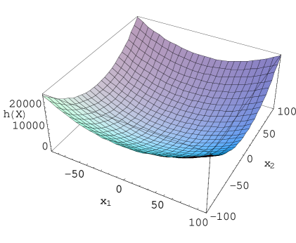
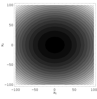
Figure 6: The log-likelihood ratio function of two features $x_{1}$ and $x_{2}$ after simultaneous diagonalization for the two covariance matrices $\Sigma_{1}$ and $\Sigma_{2}$. Left: a 3-D representation. Right: its contour plot.

Back to (15)–(16), unfortunately, a closed form integration for (15) and (16) over $x_{1}$, to obtain the marginal probabilities $f(h|\omega_{1})$ and $f(h|\omega_{2})$, is not available. However, we always can obtain a numerical solution to the problem by carrying out the integration over $x_{1}$ for every desired value of $h$. The marginal PDFs of $h$, conditional on $\omega_{1}$ and $\omega_{2}$, are obtained by the described technique and illustrated in Figures 7 (the two left figures). In addition, these two figures show the histograms of $h$ obtained from simulating testing observations from the distributions $F_{1}$ and $F_{2}$ and obtaining the log-likelihood ratio $h$ for every observation. The figures show how well both, the histogram and the mathematical solution, are highly consistent. Figure 7 (right) shows the two PDFs, together on the same scale, for the classification purpose.

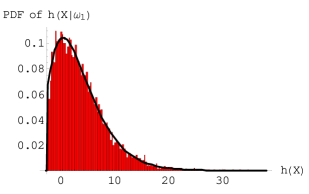
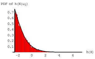
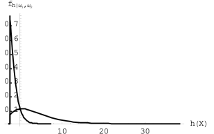
Figure 7: The PDF of the log-likelihood ratio under $\omega_{1}$ (left) and $\omega_{2}$ (middle) obtained from mathematical analysis, along with its histogram obtained from a simulation study. The same two PDFs are plotted together on the same scale (right)

It is extremely important to comment on the result illustrated in Figure 7. Although the data are coming from binormal distributions, the log-likelihood ratio is not distributed as normal distribution; both are single-tailed. Moreover, $f_{h|\omega_{2}}$, in no way, can be approximated to a normal distribution. It has an abrupt behavior that makes it resemble more the exponential distribution. This simple example provides an important caveat to the exaggerated use of normality for the log-likelihood ratio.

3 Properties of AUC Under Multinormal Assumption: expected behavior

This section contrasts Section 2. We present some of the expected behavior under the multinormal assumption of the feature vector. To exhibit the basic structure of the problem under the practical limitation of a finite-training set, we carried out simulations inspired by Chan et al. (1999) and the work of Fukunaga and Hayes (1989a, b). In our simulation, we assume that the feature vector has the multinormal distribution with the following parameters: $\mu_{1}={0}$, $\mu_{2}=c\mathbf{1}$, and $\Sigma_{1}=\Sigma_{2}=\mathbf{I}$, where $\mathbf{0}$ and $\mathbf{1}$ are the vectors all of whose components are zeros and ones respectively, $\mathbf{I}$ is the identity matrix, and $c$ is a constant used for adjusting the separation between the two classes. A fundamental measure for that is the Mahalanobis distance between the mean vectors; it is defined as:

$$\Delta=\left[{(\mu_{1}-\mu_{2}{)}^{\prime}\Sigma^{-1}(\mu_{1}-\mu_{2})}\right]^{1/2}.$$ (19)

It expresses how these two vectors are separated from each other with respect to the spread $\Sigma$. In the simulation of the present example, the Mahalanobis distance is $c^{2}p$. In this simulation, illustrated in Figure 8, the value $c$ is adjusted for every dimensionality to obtain the same asymptotic AUC that can be obtained form (8).

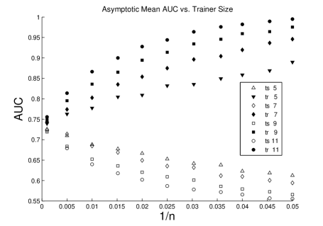
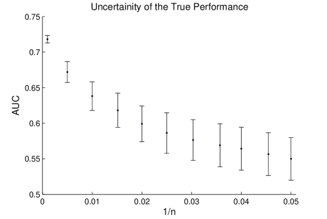
Figure 8: Classifier performance. Left: mean AUC of the Bayes classifier. For every training sample size $n$, the classifier is tested on pseudo-infinite testers (represented as “ts”) and tested as well on the same training sample ( represented as “tr”). Each curve shows the average performance over 100 MC trials. The numbers in the legend are the dimensionalities of the feature vectors. Right: uncertainty (variance) around the mean performance of the Bayes classifier, for 11 features, vs. the size of the training data set. Asymptotically, the variability vanishes.

This allows us to isolate the effect of the variation in training set sizes. Typically, the simulations described in this context used $\Delta=0.8$. For the time being, it is assumed that $n_{1}=n_{2}=n$, which is referred to as the training set size per class. For a particular dimensionality, and for particular data set size $n$, two training data sets are generated using the above parameters and distributions. When the classifier is trained, it will be tested on a pseudo-infinite test set, here 1000 cases per class, to obtain a very good approximation to the true AUC for the classifier trained on this very training data set; this is called a single realization or a Monte-Carlo (MC) trial. Many realizations of the training data sets with same $n$ are generated over MC simulation to study the mean and variance of the AUC for the Bayes classifier under this training set size. The number of MC trials used is 100.

Since any classifier is designed using a finite-size data set, its true performance—the performance obtained from expectation over the population—is dominated by the size of this set—assuming fixing the distribution of the data. When the classifier is re-designed using different training set size, the expected performance will vary. This is because the limited size training set has some, not all, of the information represented in the population. Figure 8 (left) illustrates this for the set of experiment parameters explained above, where it plots the mean AUC vs the reciprocal of the training set size under different dimensionality $p$. On the other hand, if the classifier is re-designed, using another data set having the same size, the performance will vary as well. This is because the performance measure is a function of the training data set; hence it is a random variable. Figure 8 (right) is an illustration of this fact for the special case of $p=11$, and $c=0.27$.

Several important observations can be made from these results. As was expected, for training size $n$ the mean apparent AUC, i.e., coming from testing on the same training data set, is upwardly biased from the true AUC. It should be cautioned that this is on the average, i.e., over the population of all training sets; it is possible that for a single data set (single realization) the apparent performance can be better or worse than the true one. In addition, the classifier had the same asymptotic performance, approximately 0.74, for all dimensionalities in the simulation (by construction as explained above).

4 Conclusion

First, this article introduced the binary classification problem and provided a brief account of its mathematical foundation. In this introduction we distinguished between the distribution of the input feature vector (the predictor) and the distribution of the output scoring function that will be compared to a threshold value to provide the final class prediction (the response). The distribution of the output scoring function determines the properties of the performance measure of the classifier, including the error rate, the Receiver Operating Characteristic (ROC) curve, and the Area Under the Curve (AUC), among many other measures. There is a well established literature, both theoretically and experimentally, for the performance of classification rules under the normality assumption of either the input feature vector or the output scoring function. This rich literature makes it very tempting and, in many cases very beneficial, to adopt either of these two normality assumptions. Second, the article proved with a counter example how this normality assumption of the scoring function may be severely violated under a very simple setup of normal assumption of the input feature vector. However, we frequently see the Central Limit Theorem (CLT) at work in higher dimensions driving the final scoring function towards the binormal assumption and the ROC curve towards the double-normal-deviate plot. Third, the article provided the complementary balancing message and illustrated experimentally some of the expected properties of the AUC under the multinormal assumption of the input feature vector. To recap, the article does not discourage the practitioners from using the normality assumption; however, the article calls for prudence when adopting it.

5 Acknoledgment

The author is grateful to the U.S. Food and Drug Administration (FDA) for funding an earlier stage of this project. Special thanks and gratitude, in his memorial, to Dr. Robert F. Wagner the supervisor and teacher, or Bob Wagner the big brother and friend. He reviewed a very early version of this manuscript before his passing away.

References

- Anderson (2003) Anderson, T.W., 2003. An introduction to multivariate statistical analysis. 3rd ed., Wiley-Interscience, Hoboken, N.J.
- Bishop (2006) Bishop, C.M., 2006. Pattern recognition and machine learning. Springer, New York.
- Chan et al. (1999) Chan, H.P., Sahiner, B., Wagner, R.F., Petrick, N., 1999. Classifier Design for Computer-Aided Diagnosis: Effects of Finite Sample Size on the Mean Performance of Classical and Neural Network classifiers. Medical Physics 26, 2654–2668.
- Dorfman et al. (1992) Dorfman, D.D., Berbaum, K.S., Metz, C.E., 1992. Receiver Operating Characteristic Rating Analysis - Generalization To the Population of Readers and Patients With the Jackknife Method. Investigative Radiology 27, 723–731.
- Dorfman et al. (1997) Dorfman, D.D., Berbaum, K.S., Metz, C.E., Lenth, R.V., Hanley, J.A., Abu Dagga, H., 1997. Proper Receiver Operating Characteristic Analysis: the Bigamma model. Acad Radiol 4, 138–149.
- Duda et al. (2001) Duda, R.O., Hart, P.E., Stork, D.G., 2001. Pattern classification. 2nd ed., Wiley, New York.
- Fukunaga (1990) Fukunaga, K., 1990. Introduction to statistical pattern recognition. 2nd ed., Academic Press, Boston.
- Fukunaga and Hayes (1989a) Fukunaga, K., Hayes, R.R., 1989a. Effects of Sample Size in Classifier design. Pattern Analysis and Machine Intelligence, IEEE Transactions on 11, 873–885.
- Fukunaga and Hayes (1989b) Fukunaga, K., Hayes, R.R., 1989b. Estimation of Classifier performance. Pattern Analysis and Machine Intelligence, IEEE Transactions on - 11, – 1101.
- Green and Swets (1966) Green, D.M., Swets, J.A., 1966. Signal Detection Theory and Psychophysics. Robert E. Krieger Publishing Company, Huntington, New York.
- Hájek et al. (1999) Hájek, J., Šidák, Z., Sen, P.K., 1999. Theory of rank tests. 2nd ed., Academic Press, San Diego, Calif.
- Hastie et al. (2009) Hastie, T., Tibshirani, R., Friedman, J.H., 2009. The elements of statistical learning: data mining, inference, and prediction. 2nd ed., Springer, New York.
- Jiang et al. (1996) Jiang, Y., Metz, C.E., Nishikawa, R.M., 1996. A Receiver Operating Characteristic Partial Area Index for Highly Sensitive Diagnostic tests. Radiology 201, 745–750.
- Krzanowski and Hand (2009) Krzanowski, W.J., Hand, D.J., 2009. ROC curves for continuous data. 111, CRC Press, Boca Raton.
- Metz and Pan (1999) Metz, C.E., Pan, X., 1999. “Proper” Binormal {ROC} Curves: Theory and Maximum-Likelihood Estimation. Journal of Mathematical Psychology 1, 1–33.
- Pan and Metz (1997) Pan, X., Metz, C.E., 1997. The “proper” Binormal Model: Parametric Receiver Operating Characteristic Curve Estimation With Degenerate data. Academic Radiology 4, 380.
- Randles and Wolfe (1979) Randles, R.H., Wolfe, D.A., 1979. Introduction to the theory of nonparametric statistics. Wiley, New York.
- Schott (2005) Schott, J.R., 2005. Matrix analysis for statistics. 2nd ed., Wiley, Hoboken, N.J.
- Searle (1982) Searle, S.R., 1982. Matrix algebra useful for statistics. Wiley, New York.
- Walter (2005) Walter, S.D., 2005. The Partial Area Under the Summary {ROC} curve. Statistics In Medicine 24, 2025–2040.
- Yousef (2013) Yousef, W.A., 2013. Assessing Classifiers in Terms of the Partial Area Under the Roc curve. Computational Statistics & Data Analysis 64, 51–70. URL: https://doi.org/10.1016/j.csda.2013.02.032.