Abstract

Recently, the CMS Collaboration observed the hint of a resonance decaying to two photons at about 96 GeV with a local significance of $2.8\sigma$. While it is too early to say whether this will stand the test of time, such a resonance can easily be accommodated in many extensions of the Standard Model (SM). The more challenging part is to tune such an extension so that the required number of diphoton events is reproduced. Assuming that the new resonance is a scalar, we propose that the signal may come either from an ultraviolet complete model with vectorial quarks, or a model involving gluon-scalar and photon-scalar effective operators. We then incorporate this portal to several extensions of the SM that include one or more cold dark matter candidates, and try to investigate how the existence of such a scalar resonance affects the parameter space of such models. As expected, we find that with such a scalar, the parameter space gets more constrained and hence, more tractable. We show how significant constraints can be placed on the parameter space, not only from direct dark matter searches or LHC data but also from theoretical considerations like scattering unitarity or stability of the potential, and discuss some novel features of the allowed parameter space.

1 Introduction

The existence of cold dark matter (CDM) is perhaps the biggest motivation to search for physics beyond the Standard Model (SM). The SM does not contain any suitable CDM candidate, something that is massive, and singlet under $U(1)_{\rm em}$ and $SU(3)_{\rm c}$. Any extension of the SM with a $\mathbb{Z}_{2}$ symmetry for which all the SM fields are $\mathbb{Z}_{2}$-even can potentially come to the rescue, with the CDM candidate being the lightest $\mathbb{Z}_{2}$-odd particle. The lightest neutralino of the R-parity conserving supersymmetric models, and the lightest Kaluza-Klein particle of the Universal Extra Dimension models, fall in this category. Gauge singlet objects like massive right-handed neutrinos, or additional scalars, can also fit the bill. In our subsequent discussion, we will assume a thermalised non-baryonic CDM with the density given by [1]

$$\Omega_{\rm CDM}h^{2}=0.1186\pm 0.0020\,,$$ (1)

where $h=H_{0}/100$ is the reduced Hubble constant. The existing literature is abound with the possible models of CDM, their detection strategies, and other phenomenological aspects. Let us refer the reader, in general, to some review articles [2], in particular, to Ref. [3] for the analysis of several Higgs portal CDM models, and to Ref. [4] for their collider signatures.

It is always an interesting exercise to link the CDM with some other beyond-SM signals or even motivations, like the generation of neutrino masses, or the flavour anomalies. In this paper, we will study some CDM models in conjunction with the recently observed hint of a (possibly) scalar resonance, close to $2.8\sigma$ or 98% CL, at about 96 GeV from the CMS Collaboration [5], decaying to a diphoton final state, with $\sim 370\,(1070)$ events in the 8 (13) TeV dataset. Although there has been neither confirmation nor denial from the ATLAS Collaboration, this hint has given rise to a lot of interesting theoretical speculations, and the physics implication of such a resonance in the context of beyond-SM scenarios, including its collider signatures, has been discussed in Refs. [6, 7, 8, 9, 10]. The astrophysics implications of models with a light scalar decaying into two photons have been studied in Ref. [11].

How does this new scalar, which we will call $\chi$, help in the analysis? While $\chi$—assuming that it exists—can never be a CDM candidate, it can very well be one component of a multiplet with the other component(s) constituting the dark matter, or it can be a mediator for the CDM-SM interaction. A fairly straightforward example, which we will discuss in detail, is to add a complex singlet to the SM; one of its components is the DM, while the other leads to $\chi$. The interesting part is that such a scenario reduces the number of free parameters in the model, and hence the allowed parameter space for the CDM becomes more tractable. This is, in a sense, the rationale of this paper.

In this paper, we consider three models that accommodate both $\chi$ and a prospective CDM candidate. They are, respectively,

1. Complex Scalar (CS): This consists of the SM augmented by a complex scalar singlet $S$. One of the components of $S$ mixes with the SM doublet, and these two states appear as $\chi$ and $h$, the 125 GeV Higgs boson. We further refer the reader to Refs. [11, 12, 13, 14] for more discussion on the CDM component of a complex scalar augmented SM.

2. Real Scalar with Fermion (RSF): Here one has a real gauge singlet scalar (which mixes with the SM doublet), and a vectorial gauge singlet fermion $\psi$ that plays the role of the CDM candidate.

3. Complex Scalar with Fermion (CSF): This is, in a sense, an amalgamation of the previous two models. We take a complex singlet scalar $S$ with the singlet fermion $\psi$, and consider the possibility where we have two CDM candidates, one scalar and the other fermionic. For such singlet fermionic CDM models, we refer the reader to, e.g., Refs. [15, 16, 17, 18, 19, 20]. The two-component CDM models, along with their collider signatures, have been discussed in, e.g., Refs. [21, 22, 23, 24, 25, 26].

It must be admitted at this point that these models, per se, fall short of explaining the CMS diphoton signal at 96 GeV. While the models include such a scalar, its diphoton decay width is either zero or too small to be interesting. This is because $\chi$ does not couple directly to photons (for decay) or gluons (for production), neither does it couple to the SM quarks and leptons through which production and decay can be mediated. To alleviate this shortcoming, we invoke either of these two further extensions to each of the three models, which are:

Subclass (a): The model contains an $SU(2)_{\rm L}$ singlet vectorial quark $Q$. This is in addition to the vectorial fermion in the RSF or CSF models, and may not belong to the same multiplet. To avoid direct detection at the LHC, we take, for our analysis, $M_{Q}=2$ TeV. The relevant part of the Lagrangian, including both QED and QCD interactions, looks like

$${\cal L}=\overline{Q}\left(i\gamma^{\mu}\partial_{\mu}-m_{Q}\right)Q-qe\,\overline{Q}\gamma^{\mu}QA_{\mu}-g_{s}\,\overline{Q}_{i}\gamma^{\mu}(T^{a})_{ij}Q_{j}G^{a}_{\mu}\,,$$ (2)

and once the Yukawa couplings are introduced, the physical mass $M_{Q}$ may contain, apart from $m_{Q}$, a contribution from symmetry breaking. As this is a vectorial fermion, no gauge or mixed anomaly is introduced, neither do we encounter the risk of a large nonperturbative Yukawa coupling (with the singlet scalar $\chi$) as most of the mass can originate without symmetry breaking. In our subsequent discussion, we will take its Yukawa coupling to be $\sim\frac{2}{3}$ in the RSF model and $\sim 0.95$ in the CS and CSF models, and its electric charge to be $+2e$. This correctly reproduces the number of diphoton events $\sim 370$ in the $\sqrt{s}=8$ TeV data. It could have been done with a smaller charge and a large Yukawa coupling too, but that makes the potential of the theory unstable even at the LHC scale. We will discuss these issues later.

Subclass (b): We do not invoke any extra fermion or any extra degrees of freedom; rather, in the spirit of effective theories, we integrate out the new fields and introduce two dimension-5 operators of the form $F_{\mu\nu}F^{\mu\nu}\chi$ and $G^{a}_{\mu\nu}G^{a\mu\nu}\chi$, for the photon and the gluon fields respectively, where the first term is responsible for the diphoton decay and the second term for the production of $\chi$ through gluon-gluon fusion. This is obviously not an independent subclass, as the heavy fermions of Subclass (a) can be integrated out to generate Subclass (b). On the other hand, many other extensions can also lead to such effective operators. We use the effective Lagrangian

$${\cal L}_{\rm eff}=-\frac{C_{\gamma}}{\Lambda}\,F_{\mu\nu}F^{\mu\nu}\chi-\frac{C_{g}}{\Lambda}\,G^{a}_{\mu\nu}G^{a\mu\nu}\chi\,,$$ (3)

and the Wilson coefficients (WC) $C_{\gamma}$ and $C_{g}$ reproduce the CMS diphoton rate for moderate enough values even with $\Lambda=100$ TeV, say $C_{\gamma}\sim 0.30$ and $C_{g}\sim 0.54$. One can even have higher-dimensional operators, like $F_{\mu\nu}F^{\mu\nu}S^{2}$, but their WCs will be suppressed by higher powers of $\Lambda$.

One may note here that such models, either with a vectorlike fermion or effective operators, were discussed in detail during the heydays of the now-dead 750 GeV diphoton resonance. We refer the reader to, e.g., Refs. [27] for a detailed analysis, and to Refs. [28] for its association with possible dark matter models.

We will concentrate on the allowed parameter space for all these models, taking the theoretical and experimental constraints, including the CMS data, into account. One major constraint is the stability of the potential; when the couplings evolve with energy, the potential should neither be unbounded from below, nor should the couplings blow up at the Landau pole (a more conservative statement is that they should remain perturbative). Up to what scale the potential should be well-behaved? Ideally, it is the Planck scale $M_{\rm Pl}$, but that makes the parameter space too restrictive; even the SM may not be stable up to $M_{\rm Pl}$. In fact, this scale can be anything beyond the reach of the LHC, where some new degrees of freedom appear and cure the bad behaviour of the potential. For Subclass (b), we demand that the theory be well-behaved up to the scale $\Lambda$. We take this scale to be 100 TeV for all our subsequent discussion. As we will see, the scalar couplings of the potential get bounded both from above and below with the conditions of stability and triviality. Pushing up the scale further only squeezes the parameter space, but no qualitative change takes place.

The paper is organised as follows. In Section 2, we give a brief outline of these models, including the theoretical and experimental constraints. The final parameter space for all the three models, taking into account the aforementioned constraints plus the direct CDM search results, are shown in Section 3, where we also enlist a few novel observations. Section 4 summarises and concludes the paper.

2 The Models

As mentioned in the Introduction, we will discuss three models in this Section. The common characteristics of these three models are: (i) they have one (or more) potential CDM candidate(s), and possibly some other degrees of freedom to generate the CMS diphoton signal; (ii) apart from the 125 GeV scalar resonance $h$, which is dominantly the SM doublet Higgs boson, every model is constructed in such a way as to further accommodate another scalar $\chi$ at 96 GeV. Even if the 96 GeV bump does not stand the test of time, the results, on the allowed parameter space of the CDM mass and couplings, will still be more or less valid, although some constraints will be relaxed.

The following constraints on the potential need to be considered:

• Existence of a definite ground state, which means that the potential cannot be unbounded from below along any direction in the field space. As mentioned before, we allow the possibility of some new physics to take over at a scale $\Lambda$, so all we need is a well-defined ground state of the potential up to $\Lambda$, beyond which the new physics may cure any possible malady and make the potential well-behaved. We take $\Lambda=100$ TeV.

• Partial wave unitarity, which essentially leads to the conservation of probability. For any scattering we can decompose the amplitude into partial waves

  $$A=16\pi\sum_{\ell=0}^{\infty}\,(2\ell+1)\,P_{\ell}(\cos\theta)\,a_{\ell},$$ (4)

  and by virtue of the optical theorem which relates the cross-section with the imaginary part of the amplitude for zero scattering angle, one gets

  $$|a_{\ell}|^{2}={\rm Im}\,a_{\ell}\,\,\Rightarrow\,\,{\rm Re}\,a_{\ell}\leq\frac{1}{2}\,.$$ (5)

  We will be interested in $\ell=0$ partial waves only. The best bounds are obtained when one diagonalises the $S$-matrix and uses the scattering from one eigenvector channel $|{\rm in}\rangle$ to another $|{\rm out}\rangle$. They may be the same eigenvectors. We follow Ref. [29] to get the unitarity constraints.

• Triviality, or the constraint that none of the couplings hit the Landau pole below $\Lambda=100$ TeV. As we will see later, these two conditions turn out to be almost equivalent. Stability and triviality, taken together, limit the range of the scalar parameters of the potential.

• The invisible decay width of the Higgs when light scalars and/or fermions are present in the model should be less than 19% [30]. This is relevant only if the CDM mass is less than $m_{h}/2$.

• The dominantly doublet nature of $h$, as established by the LHC data, which means that the mixing angle with the singlet scalar must be small. This necessitates the introduction of either new fermions or new effective operators to explain the $\chi\to\gamma\gamma$ decay rate.

• The constraints coming from the CDM direct detection experiments, interpreted in terms of a thermalised dark matter, as well as those coming from the relic density of the CDM, i.e., the universe must not be overclosed [31, 32, 33]. The bounds from LUX, XENON1T, and PandaX-II collaborations are quite close to each other in the CDM mass region that we are interested in. The 2018 update of XENON1T gives slightly stronger bounds [34], but does not affect our results in a significant way if $m_{\rm CDM}>m_{\chi}/2$. For $m_{\rm CDM}>m_{\chi}$, the CDM pair annihilation to $\chi\chi$ controls $\Omega_{\rm CDM}$. For $m_{b}<m_{\rm CDM}<m_{\chi}$, the CDM pair annihilation rates to $b\bar{b}$, diphoton and digluon are of the same order.

• Bounds on the oblique electroweak parameters, which, however, have a completely negligible effect if the singlet-doublet mixing is tiny, and/or the new fermion is a gauge singlet with no mixing to the SM fermions. This is true even for the new charged fermions in Subclass (a).

The parameter space is constrained assuming the CDM candidate(s) being thermalised and satisfying the relic density limit, i.e., there are no other particles that contribute to the relic density. To compute the relic density one solves the Boltzmann equation [35] for $Y=n/s$, where $n$ is the number density and $s$ is the entropy density, and calculates the thermal averaged cross-section. Assuming a scalar CDM $S$ of mass $m_{S}$ and a coupling of the form $(\delta_{2}/4)\Phi^{\dagger}\Phi S^{2}$, the spin-independent CDM-nucleon cross-section is given by

$$\sigma_{SI}=\frac{\delta_{2}^{2}m_{N}^{4}f^{2}}{16\pi m_{S}^{2}m_{h}^{4}}\,,$$ (6)

where $m_{N}$ is the nucleon mass, and $f$ is the nuclear form factor, often taken to be $\sim\frac{1}{3}$ [36]. In this paper, we take the CDM to be thermalised, and find those regions of the parameter space that reproduce the correct CDM density. There can also be loop-induced CDM-nucleus scattering diagrams [37]. However, the loop suppression makes them negligible compared to the tree-level amplitudes. If the CDM is a scalar, the loop amplitude is a few orders of magnitude smaller than the tree-level one. For a fermionic CDM $\psi$, the Higgs-$\psi$ coupling is suppressed by the scalar mixing angle, but even then the loop suppression works in favour of the tree-level amplitudes for the mass ranges that we are interested in.

Before we go into the three models, let us have a brief recapitulation of the Real Singlet (RS) model, which is SM plus a real gauge singlet scalar $S$. The scalar potential can be written as

$$V(\Phi,S)_{\rm RS}=-\frac{m^{2}}{2}\Phi^{{\dagger}}\Phi+\frac{b_{2}}{4}S^{2}+\frac{\lambda}{4}\left(\Phi^{{\dagger}}\Phi\right)^{2}+\frac{\delta_{2}}{4}\Phi^{{\dagger}}\Phi S^{2}+\frac{d_{2}}{16}S^{4}\,,$$ (7)

where $S$-odd terms are banished from the potential by a $\mathbb{Z}_{2}$ symmetry: $S\to-S$. We will denote the CP-even neutral component of $\Phi$ by $\phi$, with

$$\langle\phi\rangle\equiv v=246~{}{\rm GeV}\,.$$ (8)

In the absence of $\Phi$-$S$ mixing, $\phi=h$, where $h$ is the physical 125 GeV scalar resonance.

If $S$ does not get any vacuum expectation value (VEV), it can act as a potential CDM candidate. However, as has been shown in Refs. [35, 38, 39, 40], the allowed region for $m_{S}<m_{h}$ is rather fine-tuned; the CDM solution survives only in a narrow resonance region around $m_{S}\approx m_{h}/2$. There are other allowed regions for large values of $m_{S}$, like $m_{S}>1$ TeV, where $S$ can be a viable CDM candidate. If we allow $S$ to be a component of CDM, and not the only constituent, the allowed region starts from $m_{h}\approx m_{S}$. All these situations have been extensively explored. We will not discuss this model any further, but we would like to have a digression here on the CMS signal, which is applicable to all the other models that we discuss.

2.1 Digression: The CMS diphoton signal

If $S$ mixes with the SM doublet $\Phi$, it cannot be a CDM candidate, but can the lighter mass eigenstate, which is dominantly a singlet, act as $\chi$? The answer, unfortunately, is no; the mixing must be small to keep the doublet nature of $h$ consistent with the LHC data, and that makes both the production cross-section, as well as the diphoton decay width, so small as to be completely unobservable at the LHC. We may refer the reader to Ref. [11] for further discussion.

Introduction of another vector singlet quark $Q$ with an electric charge $+q$ solves the problem. Apart from Eq. (2), we add a Yukawa term to the Lagrangian:

$${\cal L}_{1}=-h_{Q}\,\overline{Q}QS\,.$$ (9)

The production cross-section for $gg\to\chi$ is given by

$$\sigma(gg\to\chi)=\frac{\alpha_{s}^{2}}{576\,\pi}\,h_{Q}^{2}\,\cos^{2}\alpha\,\frac{m_{\chi}^{2}}{M_{Q}^{2}}\,\frac{d{\cal L}^{gg}}{dm_{\chi}^{2}}\,,$$ (10)

where $d{\cal L}^{gg}/dm_{\chi}^{2}$ is the gluon luminosity using the MSTW2008NLO parton distribution [41], and $\alpha$ is the singlet-doublet mixing angle. The decay width of $\chi\to\gamma\gamma$ is

$$\Gamma(\chi\rightarrow\gamma\gamma)=\frac{N_{c}^{2}\alpha_{\rm em}^{2}q^{4}}{72\pi^{3}}\,h_{Q}^{2}\cos^{2}\alpha\,\frac{m_{\chi}^{3}}{M_{Q}^{2}}\,.$$ (11)

To generate the required number of events, we take $h_{Q}\approx\frac{2}{3}$ and $|q|=2$, with which one has about 370 (1070) events for $\sqrt{s}=8\,(13)$ TeV. If there are two singlets, as in the CS and CSF models, the Yukawa interaction is of the form $(h_{Q}/\sqrt{2})\,\bar{Q}Q(S_{1}+iS_{2})$, and so we need to scale up $h_{Q}$ by $\sqrt{2}$ to $h_{Q}\approx 0.95$. With lower values of $|q|$, one needs higher $h_{Q}$, but this makes the potential unstable before 100 TeV, through the renormalisation group evolution of the singlet quartic coupling $d_{2}$, with a contribution going as $-h_{Q}^{4}$.

Alternatively, one may introduce two dimension-5 operators, as shown in Eq. (3). Two representative benchmark values for $(C_{\gamma},C_{g})$ to generate required number of events may be taken as $(0.30,0.54)$ and $(0.28,0.34)$ for $\sqrt{s}=8$ TeV and $\sqrt{s}=13$ TeV respectively.

We will now briefly discuss our models, with the implicit understanding that such a mechanism to generate the required number of $\chi\to\gamma\gamma$ decays is added to all of them. One important point to note right here is that the CDM mass must have a lower bound of approximately $m_{\chi}/2\approx 48$ GeV. For a lighter CDM, $\chi$ dominantly decays to a pair of CDM, which suppresses the diphoton branching ratio by a few orders of magnitude.

2.2 The Complex Scalar Model (CS)

Extending the scalar sector by a complex singlet $S\equiv(S_{1}+iS_{2})/\sqrt{2}$, the most general renormalisable potential is of the form [42]

$$V(\Phi,S) = -\frac{m^{2}}{2}\Phi^{{\dagger}}\Phi+\frac{\lambda}{4}\left(\Phi^{{\dagger}}\Phi\right)^{2}+\left(\frac{\delta_{1}}{4}e^{i\theta_{\delta_{1}}}\Phi^{{\dagger}}\Phi S+{\rm c.c}\right)+\frac{\delta_{2}}{2}\Phi^{{\dagger}}\Phi\mid S\mid^{2}+$$ (12)

$$\left(\frac{\delta_{3}}{4}e^{i\theta_{\delta_{3}}}\Phi^{{\dagger}}\Phi S^{2}+{\rm h.c}\right)+\left(a_{1}e^{i\theta_{a_{1}}}S+{\rm h.c}\right)+\left(\frac{b_{1}e^{i\theta_{b_{1}}}}{4}S^{2}+{\rm h.c}\right)+$$

$$\frac{b_{2}}{2}\mid S\mid^{2}+\left(\frac{c_{1}e^{i\theta_{c_{1}}}}{6}S^{3}+{\rm h.c}\right)+\left(\frac{c_{2}e^{i\theta_{c_{2}}}}{6}S\mid S\mid^{2}+{\rm h.c}\right)+$$

$$\left(\frac{d_{3}e^{i\Phi_{d_{3}}}}{8}S^{2}\mid S\mid^{2}+{\rm h.c}\right)+\frac{d_{2}}{4}\mid S\mid^{4}\,,$$

where the couplings are taken to be real apart from an explicit phase factor, generically written as $\exp(i\theta)$, with $0\leq\theta\leq\pi$. Apart from this, one should include the Yukawa coupling with $Q$:

$${\cal L}_{1}=-\frac{h_{Q}}{\sqrt{2}}\,\overline{Q}\left(S_{1}+i\gamma_{5}S_{2}\right)Q\,,$$ (13)

or suitable effective operators for Subclass (b). We will first try to confine ourselves to a simpler case, by reducing the number of independent parameters through a global $U(1)$ symmetry on $S$: $S\to S\exp(i\zeta)$. This simplifies the potential to

$$V(\Phi,S)=-\frac{m^{2}}{2}\Phi^{{\dagger}}\Phi+\frac{\lambda}{4}\left(\Phi^{{\dagger}}\Phi\right)^{2}+\frac{\delta_{2}}{2}\Phi^{{\dagger}}\Phi\mid S\mid^{2}+\frac{b_{2}}{2}\mid S\mid^{2}+\frac{d_{2}}{4}\mid S\mid^{4}\,,$$ (14)

but leads to a massless Goldstone boson in the spectrum when the symmetry breaks spontaneously to give $S$ a VEV. To avoid this, we introduce a soft $U(1)$ breaking term (but still keeping the $\mathbb{Z}_{2}$ of $S\to-S$ intact) in the potential:

$$V_{\rm CS}(\Phi,S)=-\frac{m^{2}}{2}\Phi^{{\dagger}}\Phi+\frac{\lambda}{4}\left(\Phi^{{\dagger}}\Phi\right)^{2}+\frac{\delta_{2}}{2}\Phi^{{\dagger}}\Phi\mid S\mid^{2}+\frac{b_{2}}{2}\mid S\mid^{2}+\frac{d_{2}}{4}\mid S\mid^{4}+\left(\frac{b_{1}}{4}e^{i\theta}S^{2}+{\rm h.c.}\right)\,,$$ (15)

so that $S_{2}$ becomes a pseudo Nambu-Goldstone boson with a mass proportional to $b_{1}$. The phase $\theta$ helps in realising the vacuum alignment condition. We take $\theta=\pi$ and let $S_{1}$ get the VEV:

$$\langle S\rangle=\frac{1}{\sqrt{2}}\langle S_{1}\rangle=s_{1}/\sqrt{2}\,.$$ (16)

In terms of the component fields, the potential is

$$V_{\rm CS}(\phi,S_{1},S_{2})=-\frac{m^{2}}{4}\phi^{2}+\frac{\lambda}{16}\phi^{4}+\frac{\delta_{2}}{8}\phi^{2}\left(S_{1}^{2}+S_{2}^{2}\right)+\frac{b_{2}}{4}\left(S_{1}^{2}+S_{2}^{2}\right)+\frac{d_{2}}{16}\left(S_{1}^{2}+S_{2}^{2}\right)^{2}-\frac{b_{1}}{4}\left(S_{1}^{2}-S_{2}^{2}\right)\,,$$ (17)

with the extremisation conditions

$$\frac{\partial V}{\partial\phi} = -\frac{m^{2}}{2}\phi+\frac{\lambda\phi^{3}}{4}+\frac{\delta_{2}}{4}\phi(S_{1}^{2}+S_{2}^{2})=0\,,$$

$$\frac{\partial V}{\partial S_{1}} = \frac{S_{1}}{2}\left(b_{2}-b_{1}+\frac{\delta_{2}\phi^{2}}{2}+\frac{d_{2}}{2}(S_{1}^{2}+S_{2}^{2})\right)=0\,,$$

$$\frac{\partial V}{\partial S_{2}} = \frac{S_{2}}{2}\left(b_{2}+b_{1}+\frac{\delta_{2}}{2}\phi^{2}+\frac{d_{2}}{2}(S_{1}^{2}+S_{2}^{2})\right)=0\,.$$ (18)

Note that the terms of the RS and the CS potentials have been written in such a way as to ensure identical CDM couplings with the Higgs as well as its self-coupling.

Obviously, the solution with $\langle\phi\rangle=v=0$ is not physical. For $v\not=0$, there can be two possible cases that will give rise to a CDM candidate: (i) $s_{1}=s_{2}=0$, and $s_{1}\not=0$, $s_{2}=0$. In the first case, there is no mixing between $\phi$ and $S_{1,2}$, and hence no $\chi$, so we will drop that from our focus. Only the second case is interesting, so let us treat that in more detail.

The conditions $v\not=0$, $s_{1}\not=0$, $s_{2}=0$ lead to

$$s_{1}^{2} = \frac{2\lambda\left(b_{2}-b_{1}\right)+2\delta_{2}m^{2}}{\delta_{2}^{2}-\lambda d_{2}}\,,$$

$$v^{2} = \frac{2\delta_{2}\left(b_{2}-b_{1}\right)+2d_{2}m^{2}}{\lambda d_{2}-\delta_{2}^{2}}\,,$$ (19)

thus ensuring that the four minima at $(\pm\sqrt{v^{2}},\pm\sqrt{s_{1}^{2}})$ are of equal depth, which is a consequence of the still-intact $\mathbb{Z}_{2}$ symmetry.

The couplings can be further constrained from the existence of a well-defined ground state:

$$\lambda>0\,,\ \ \ d_{2}>0\,,\ \ \ \lambda d_{2}>\delta_{2}^{2}\,.$$ (20)

The mass matrix for the neutral scalars is

$$M^{2}=\frac{1}{2}\begin{pmatrix}\lambda v^{2}&\delta_{2}vs_{1}&0\cr\delta_{2}vs_{1}&d_{2}s_{1}^{2}&0\cr 0&0&2b_{1}\end{pmatrix}\,.$$ (21)

with the mass eigenvalues

$$m^{2}_{h,\chi} = \frac{\lambda v^{2}}{4}+\frac{d_{2}s_{1}^{2}}{4}\pm\sqrt{\left(\frac{\lambda v^{2}}{4}-\frac{d_{2}s_{1}^{2}}{4}\right)^{2}+\frac{\delta_{2}^{2}v^{2}s_{1}^{2}}{4}}\,,$$

$$m^{2}_{S_{2}} = b_{1}\,.$$ (22)

$S_{2}$ is a stationary state itself; there is no mixing with the other scalars as $s_{2}=0$.

The $h$-$\chi$ mixing angle $\alpha$ is given by

$$\tan{(2\alpha)}=\frac{2\delta_{2}vs_{1}}{\lambda v^{2}-d_{2}s_{1}^{2}}\,.$$ (23)

For the analysis, it is helpful to express the parameters of the potential, namely, $\lambda$, $d_{2}$, $\delta_{2}$, $m$, $b_{2}$, and $b_{1}$, in terms of the VEVs $v$ and $s_{1}$, the mixing angle $\alpha$, and the three masses $m_{h}$, $m_{\chi}$ and $m_{S_{2}}$. Among these, $m_{h}$, $m_{\chi}$, and $v$ are known, so there are only three free parameters, including $\alpha$, which is known to be small.

The transformation equations between the two bases are

$$\lambda = \frac{2}{v^{2}}\left(m_{h}^{2}\cos^{2}\alpha+m_{\chi}^{2}\sin^{2}\alpha\right)\,,$$

$$d_{2} = \frac{2}{s_{1}^{2}}\left(m_{h}^{2}\sin^{2}\alpha+m_{\chi}^{2}\cos^{2}\alpha\right)\,,$$

$$\delta_{2} = \frac{\left(m_{h}^{2}-m_{\chi}^{2}\right)\,\sin(2\alpha)}{vs_{1}}\,,$$

$$m^{2} = \frac{1}{2}\left(\delta_{2}s_{1}^{2}+\lambda v^{2}\right)\,,$$

$$b_{1}-b_{2} = \frac{1}{2}\left(d_{2}s_{1}^{2}+\delta_{2}v^{2}\right)\,,$$

$$b_{1} = m_{S_{2}}^{2}\,.$$ (24)

We would also like to see how the dimensionless couplings evolve with energy. For this, we incorporate the explicit introduction of the vectorial quark $Q$, i.e., Subclass (a), and will do the same thing for the other two models. The one-loop $\beta$-functions are [43]

$$16\pi^{2}\beta_{d_{2}} = 5d_{2}^{2}+2\delta_{2}^{2}+12d_{2}h_{Q}^{2}-24h_{Q}^{4}\,,$$

$$16\pi^{2}\delta_{2} = \delta_{2}\left(2d_{2}+2\delta_{2}-\frac{3}{2}g_{1}^{2}-\frac{9}{2}g_{2}^{2}+6h_{Q}^{2}+3\lambda+6g_{t}^{2}\right)\,,$$

$$16\pi^{2}\beta_{\lambda} = \left(\delta_{2}^{2}+\frac{3}{2}g_{1}^{4}+3g_{1}^{2}g_{2}^{2}+\frac{9}{2}g_{2}^{4}-3g_{1}^{2}\lambda-9g_{2}^{2}\lambda+6\lambda^{2}+12\lambda g_{t}^{2}-24g_{t}^{4}\right)$$ (25)

$$16\pi^{2}\beta_{h_{Q}} = 4h_{Q}^{3}-8h_{Q}\,\left(3g_{1}^{2}+g_{3}^{2}\right)\,.$$ (26)

with $\beta_{x}=dx/dt$, and $t\equiv\ln(q/q_{0})$, where $q_{0}$ is some reference scale to set the boundary conditions on the couplings, and $q$ is the relevant energy scale where they are measured. Higher orders do not affect our results in any appreciable way. We must ensure that nowhere in the parameter space the triviality bound is reached below 100 TeV.

The parameter space becomes more complicated with the introduction of several new couplings if we allow the breaking of the $\mathbb{Z}_{2}$ symmetry. However, qualitatively it does not add much over the parameter space of the CS model that we will discuss in the next Section. One important modification is that the vacua are no longer degenerate, and one has to put the additional constraint that either the SM vacuum is the deepest one, or it is a false vacuum with the tunnelling time larger than the age of the universe. We will not discuss the $\mathbb{Z}_{2}$ breaking case any further.

2.3 Real singlet scalar with vectorial fermion (RSF)

Let us add one vector singlet fermion $\psi$ to the real singlet model of Eq. (7). This leads to the generalised potential

$$V(\Phi,S,\psi)=-\frac{m^{2}}{2}\Phi^{{\dagger}}\Phi+\frac{\lambda}{4}\left(\Phi^{{\dagger}}\Phi\right)^{2}+\frac{\delta_{2}}{4}\Phi^{{\dagger}}\Phi S^{2}+\frac{b_{2}}{4}S^{2}+\frac{d_{2}}{16}S^{4}+m_{\psi}\bar{\psi}\psi+(Y/\sqrt{2})\,\bar{\psi}\psi S\,,$$ (27)

as well as the fermionic with $Y$ being the Yukawa coupling, whose presence already breaks the ${\mathbb{Z}}_{2}$ symmetry of $S\to-S$. The CDM candidate, $\psi$, is stable as long as it does not mix with the neutrinos. For Subclass (a), one should also add the Yukawa term in Eq. (2).

Using the same notation as for the CS model, we get the scalar mass eigenstates as

$$m^{2}_{h,\chi}=\frac{1}{4}\left[\lambda v^{2}+d_{2}s_{1}^{2}\pm\sqrt{\left(\lambda v^{2}-d_{2}s_{1}^{2}\right)^{2}+4\delta_{2}^{2}v^{2}s_{1}^{2}}\right]\,,$$ (28)

with the mixing angle

$$\tan{(2\alpha)}=\frac{2\delta_{2}vs_{1}}{\lambda v^{2}-d_{2}s_{1}^{2}}\,.$$ (29)

The fermion $\psi$ is the CDM candidate, whose mass is $m_{\rm CDM}=m_{\psi}+Ys_{1}/\sqrt{2}$.

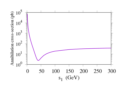
Figure 1: The dark matter annihilation cross-section as a function of the singlet scalar VEV, $s_{1}$, in the RSF model. The cross-section dips at $s_{1}\sim 50$ GeV, due to destructive interference of the $s$- and $t$-channel amplitudes. For more details, see text. The typical annihilation cross-section for WIMP-like CDM is ${\cal O}(10^{-8})$ GeV^-2 or a few pb, although it depends on the mass of the CDM and its freeze-out temperature.

The inclusion of $\psi$ helps in stabilising the potential: The negative contribution in the $\beta$-function keeps $\delta_{2}$ and $d_{2}$ in check, which in turn affects the running of $\lambda$. The one loop $\beta$-functions are given by

$$16\pi^{2}\beta_{d_{2}} = \frac{9}{2}d_{2}^{2}+2\delta_{2}^{2}+24d_{2}h_{Q}^{2}-96h_{Q}^{4}+4d_{2}Y^{2}-8Y^{4}\,,$$

$$16\pi^{2}\beta_{\delta_{2}} = \delta_{2}\left(\frac{3}{2}d_{2}+2\delta_{2}-\frac{3}{2}g_{1}^{2}-\frac{9}{2}g_{2}^{2}+12h_{Q}^{2}+2Y^{2}+3\lambda+6g_{t}^{2}\right)\,,$$

$$16\pi^{2}\beta_{\lambda} = \frac{\delta_{2}^{2}}{2}+\frac{3}{2}g_{1}^{4}+3g_{1}^{2}g_{2}^{2}+\frac{9}{2}g_{2}^{4}-\left(3g_{1}^{2}+9g_{2}^{2}\right)\lambda+6\lambda^{2}+12\lambda g_{t}^{2}-24g_{t}^{4}\,,$$

$$16\pi^{2}\beta_{h_{Q}} = 9h_{Q}^{3}+h_{Q}Y^{2}-8h_{Q}\,\left(3g_{1}^{2}+g_{3}^{2}\right)\,,$$

$$16\pi^{2}\beta_{Y} = Y\,\left(6h_{Q}^{2}+\frac{5}{2}Y^{2}\right)\,.$$ (30)

With more scalars added to the SM, the scalar quartic couplings tend to blow up, hitting the Landau pole much below the Planck scale. One has to choose points in the parameter space such that not only Eq. (1) is satisfied, but the couplings also remain perturbative up to $\Lambda=100$ TeV. As we will see later, this puts some nontrivial constraints on the parameter space.

In Fig. 1, we show the annihilation cross-section of the CDM, $\psi\bar{\psi}\to X$, where $X$ is any allowed SM particle-antiparticle pair, or even $\chi\chi$. Note that $\psi$ is non-relativistic even at freeze-out and hence its number density goes as $T^{3/2}\exp(-m_{\psi}/T)$, where $T$ is the temperature of the CDM. The $s$-channel amplitude is mediated by the singlet scalar $S$ (and hence by $h$ and $\chi$ after mixing), while the $t$-channel process is simply $\psi\bar{\psi}\to SS$. The amplitudes depend on the Yukawa coupling $Y$. For this plot, the CDM mass is kept fixed at 100 GeV, so the cross-section, in turn, depends on the VEV $s_{1}$. We find that there is a dip in the cross-section near $s_{1}\approx 50$ GeV, as the $s$- and $t$-channel amplitudes interfere destructively. The position of the dip, obviously, will depend on the chosen value of $m_{\psi}$ and $Y$. This fact will be relevant when we study the allowed parameter space.

2.4 Complex singlet scalar with vectorial fermion (CSF)

Analogous to RSF, the particle content is that of the CS model plus the singlet vectorial fermion $\psi$. The generalised potential looks like

$$V_{\rm CSF}(\Phi,S,\psi)=V_{\rm CS}+m_{\psi}\bar{\psi}\psi+\frac{Y}{\sqrt{2}}\,\left(\bar{\psi}\psi S_{1}+i\bar{\psi}\gamma_{5}\psi S_{2}\right)\,,$$ (31)

augmented by the Yukawa term in Eq. (13), where $V_{\rm CS}$ is given by Eq. (15). This can lead to two distinct possibilities:
(i) $\langle\Phi\rangle=v/\sqrt{2}$, $\langle S_{1}\rangle=s_{1}$, $\langle S_{2}\rangle=0$: The scalar sector will be completely identical to that of the CS model, and there are two possible CDM candidates, namely, $\psi$ and $S_{2}$. Based on the number of CDM candidates, we will call this model CSF-2.
(ii) $\langle S_{2}\rangle=s_{2}\not=0$. This leads to $\phi$-$S_{1}$-$S_{2}$ mixing. In other words, the field $S$ gets a complex VEV $s=s_{1}+is_{2}$. The only CDM candidate is $\psi$. This will, therefore, be called the CSF-1 model

The phenomenology of CSF-1 is more or less the same as that of RSF, so we will concentrate on the CSF-2 model. The scalar mass eigenstates are given by Eq. (28), as well as $m^{2}_{S_{2}}=b_{1}$, while the mass of $\psi$ is, as before, $m_{\rm CDM}=m_{\psi}+Ys_{1}/\sqrt{2}$. The $h$-$\chi$ mixing angle $\alpha$ is the same as shown in Eq. (29). The one loop $\beta$-functions are:

$$16\pi^{2}\beta_{d_{2}} = 5d_{2}^{2}+2\delta_{2}^{2}+12d_{2}h_{Q}^{2}-24h_{Q}^{4}+4d_{2}Y^{2}-8Y^{4}\,,$$

$$16\pi^{2}\beta_{\delta_{2}} = \delta_{2}\,\left(2d_{2}+2\delta_{2}-\frac{3}{2}g_{1}^{2}-\frac{9}{2}g_{2}^{2}+6h_{Q}^{2}+2Y^{2}+3\lambda+6g_{t}^{2}\right)\,,$$

$$16\pi^{2}\beta_{\lambda} = \delta_{2}^{2}+\frac{3}{2}g_{1}^{4}+3g_{1}^{2}g_{2}^{2}+\frac{9}{2}g_{2}^{4}-\left(3g_{1}^{2}+9g_{2}^{2}\right)\lambda+6\lambda^{2}+12\lambda g_{t}^{2}-24g_{t}^{4}\,,$$

$$16\pi^{2}\beta_{h_{Q}} = 4h_{Q}^{3}+h_{Q}Y^{2}-8h_{Q}\,\left(3g_{1}^{2}+g_{3}^{2}\right)\,,$$

$$16\pi^{2}\beta_{Y} = Y\left(3h_{Q}^{2}+2Y^{2}\right)\,.$$ (32)

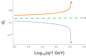
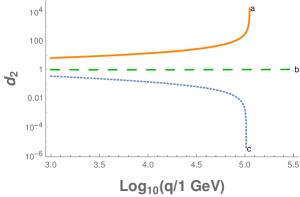
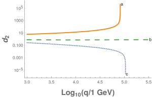
Figure 2: Renormalisation group flow of the scalar quartic coupling $d_{2}$ in the three models: CS (left), RSF (centre), and CSF (right). The upper and lower lines in each plot indicate $d_{2}$ (1 TeV) for which the model ceases to be valid at 100 TeV, from triviality and stability respectively. The middle dashed line indicates a typical value for which the model is stable up to a very high scale, $10^{8}$–$10^{10}$ GeV.

Model	Line	$d_{2}$	$\delta_{2}$	$Y$	$\alpha$	$h_{Q}$
	Upper	6.10	0.094
CS	Middle	1.21	0.042	—	0.10	0.95
	Lower	0.29	0.021
	Upper	6.44	0.049
RSF	Middle	1.00	0.019	0.85	0.05	0.68
	Lower	0.36	0.011
	Upper	6.33	0.048
CSF	Middle	0.83	0.017	0.70	0.05	0.95
	Lower	0.28	0.010

Table 1: Parameter values for the plots of Fig. 2, with $|q|=2$ for all the plots to reproduce the CMS signal strength. The values of $Y$ and $\alpha$ are kept fixed for all the lines of any particular model.

In Fig. 2, we show how the scalar quartic $d_{2}$ is bounded by triviality and stability of the potential in all the three models. Taking $\Lambda=100$ TeV, up to which we demand the theory to hold, one obtains upper and lower limits on $d_{2}$ at 1 TeV. This, of course, depends on the couplings $\delta_{2}$ and $Y$ (for RSF and CSF), as well as the mixing angle $\alpha$, which is shown in Table 1. More important is to note that the limits also depend on the Yukawa coupling $h_{Q}$, whose value one may extract from the CMS signal strength. The values have been chosen in such a way that they satisfy $\Omega_{\rm CDM}h^{2}\leq 0.12$.

3 Constraints on the parameter space

The major constraints on the parameter space have been enlisted in Section 2. We assume a thermalised dark matter distribution and use micrOMEGAs v5.0.8 [44] to obtain the relic density as well as the CDM-nucleon scattering cross-section. The one-loop RG equations were solved through SARAH v4.14.1 [45], and the unitarity constraints were found from Ref. [29]. The rest of the constraints were dealt with analytically.

3.1 The CS model

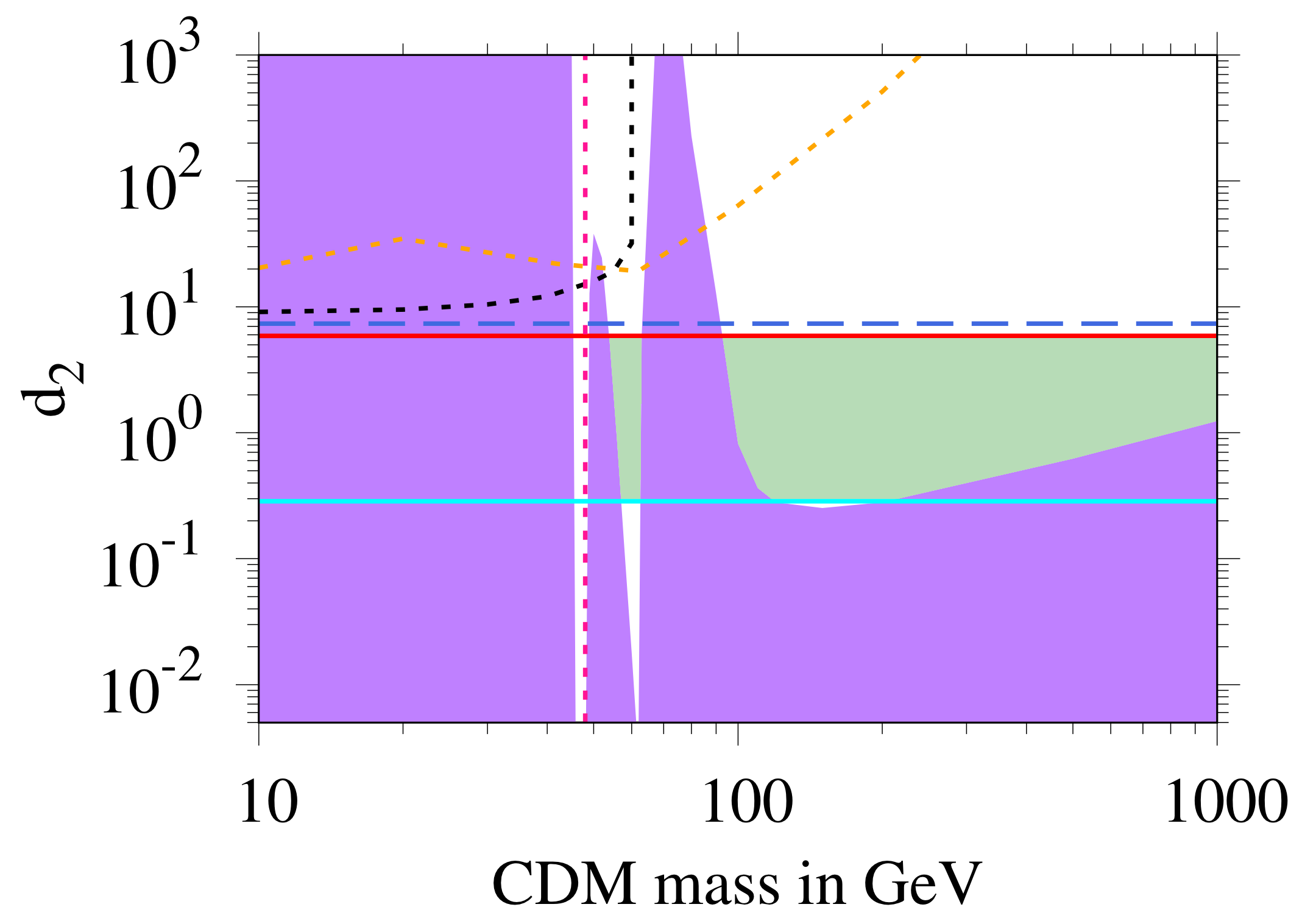
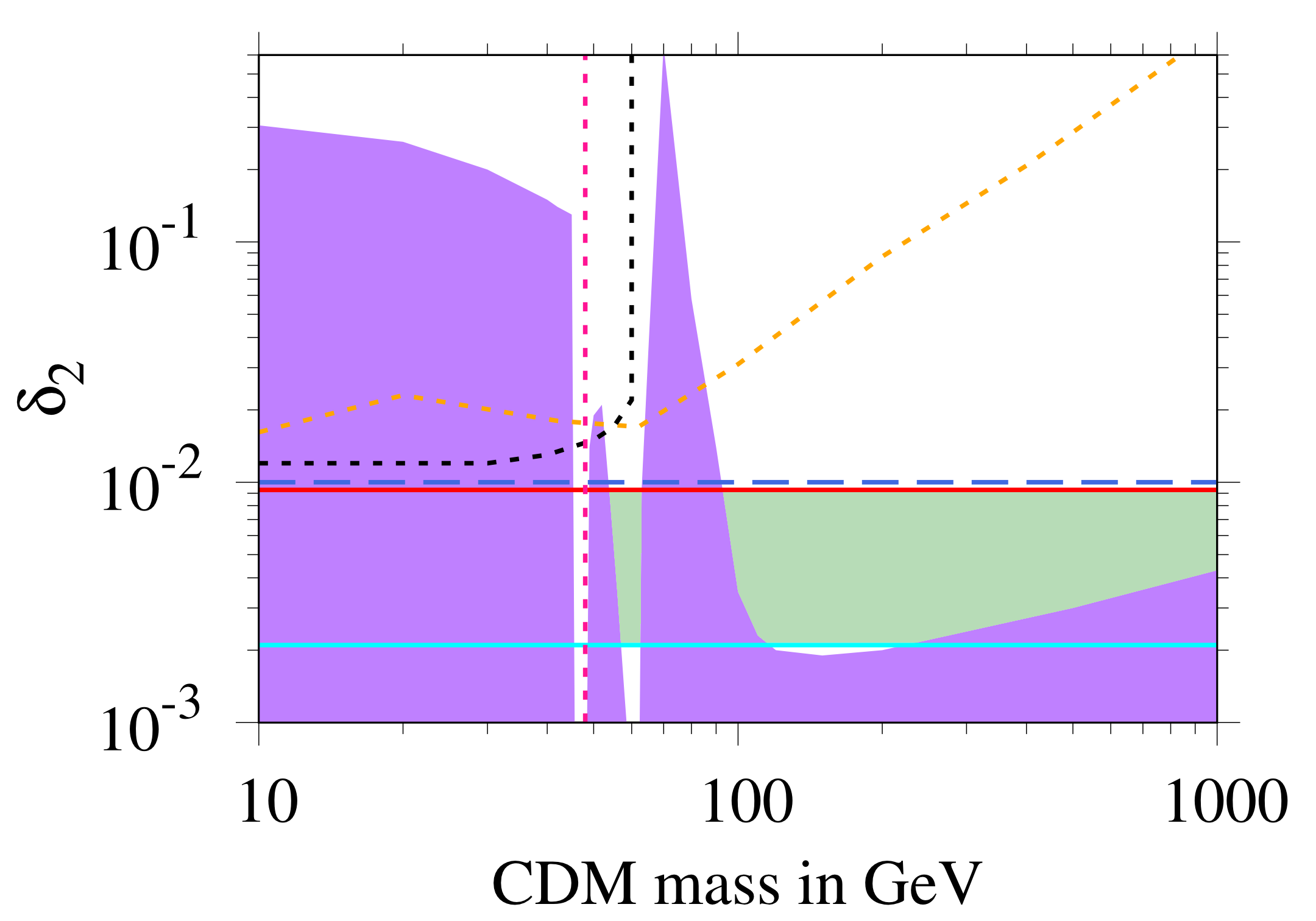
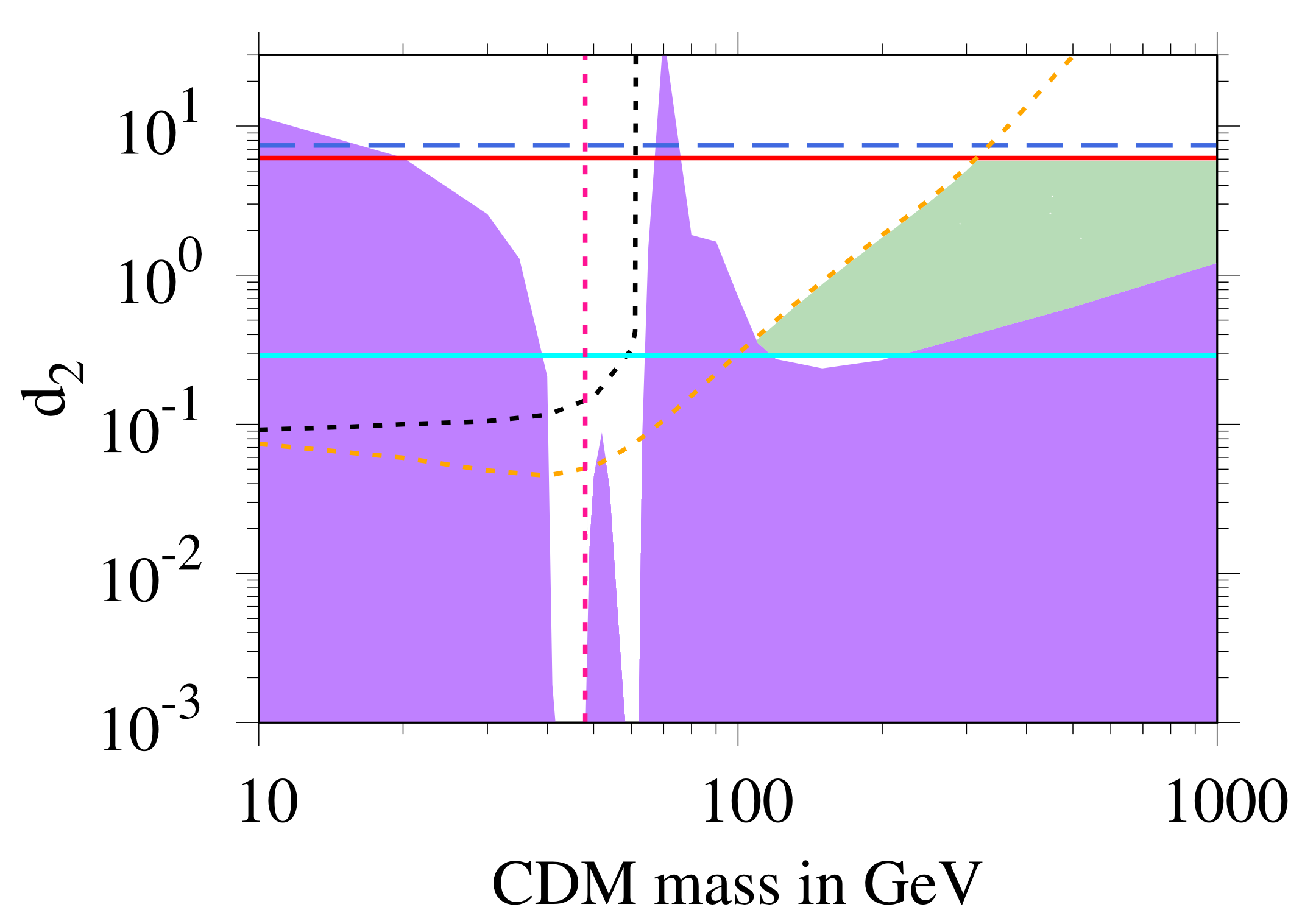
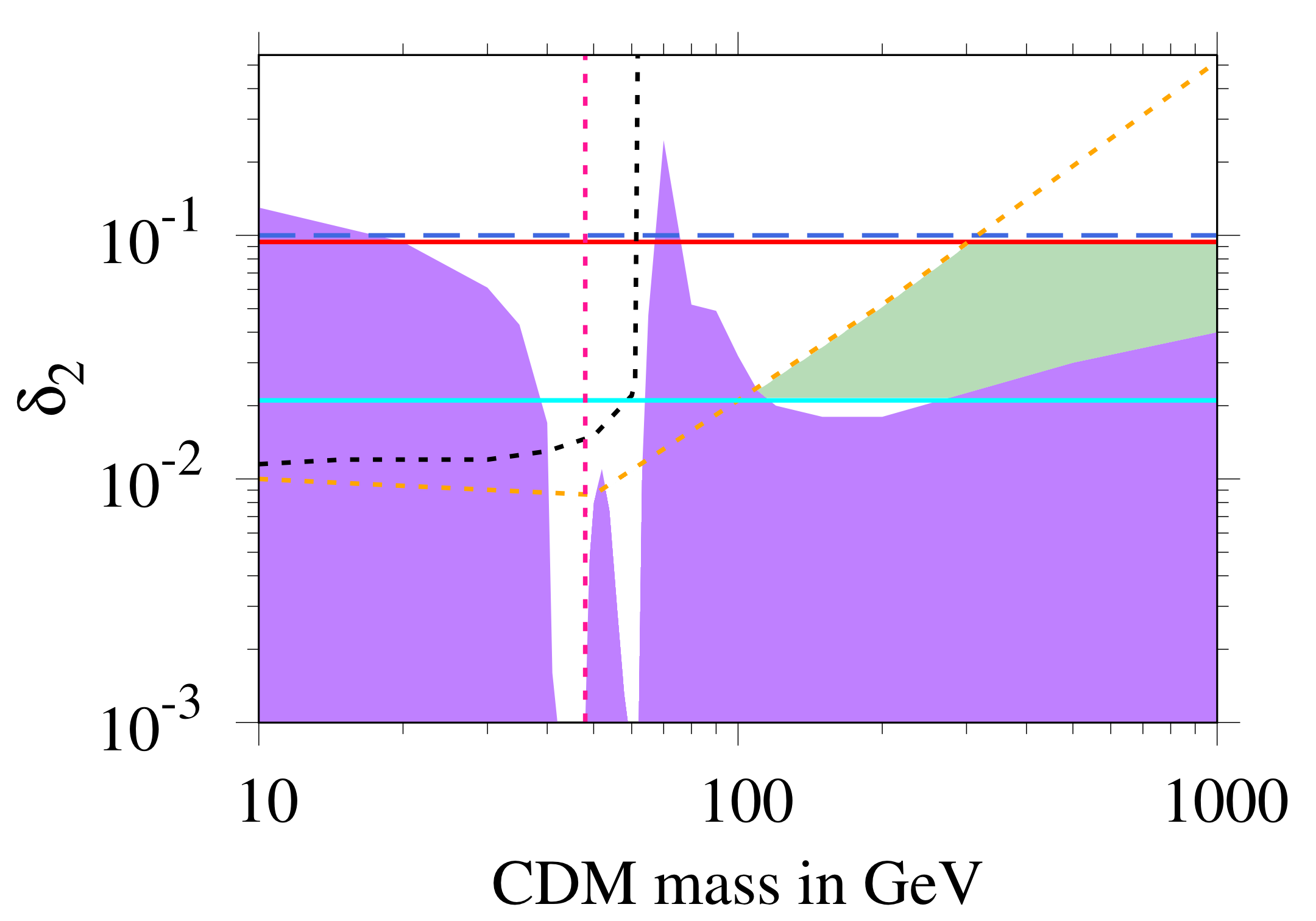
Figure 3: The allowed parameter space for the CS model with $\alpha=0.01$. The scalar $S_{2}$ is the CDM candidate. The purple region is excluded from overclosure ($\Omega h^{2}\geq 0.12$), the region above the dashed black line is excluded from the invisible decay of $h$ [BR$(h\to{\rm invis})<0.19$], the region above the dashed orange line is excluded from the direct detection experiments, the region above the long-dashed blue line is excluded from the scattering unitarity constraints, the region above the solid red line is excluded from the triviality constraint (no Landau pole before 100 TeV), and the region below the horizontal cyan line is excluded from the stability of the potential. The left region of the vertical dashed line at 48 GeV is ruled out from the CMS diphoton signal. The light green region is allowed from all theoretical and experimental constraints.

Figure 4: The CS parameter space plot as in Fig. 4, but for $\alpha=0.1$. Legends remain the same.

Let us first explain the strategy for the CS model. As $m_{\chi}$ is fixed at 96 GeV, only two relevant free parameters remain: $\alpha$ and $s_{1}$. From Eq. (24), one can trade them for the scalar quartics $d_{2}$ and $\delta_{2}$. The third free parameter, $b_{1}$, is nothing but the mass squared of the CDM, i.e., $S_{2}$. Note that throughout our discussion, we keep $h_{Q}$ fixed at $0.95$ with $|q|=2$. If the CMS signal strength changes, so will $h_{Q}$, and therefore the horizontal cyan line of all these plots that denotes the lower bound on the scalar quartics will shift its position. If the signal disappears altogether, the vertical line at $m_{\rm CDM}=48$ GeV will no longer be there; we display the low-mass CDM region keeping that possibility in mind.

The relic density, therefore, is a function of $d_{2}$, $\delta_{2}$, and $m_{S_{2}}$. The mixing angle $\alpha$ has to be small enough to maintain the dominantly doublet nature of $h$. Thus, a good strategy is to fix $\alpha$ and see what values of $s_{1}$ produce the correct relic density for different CDM masses $m_{S_{2}}$. Alternatively, one can show the constraints taking $d_{2}$ or $\delta_{2}$ as the free parameter.

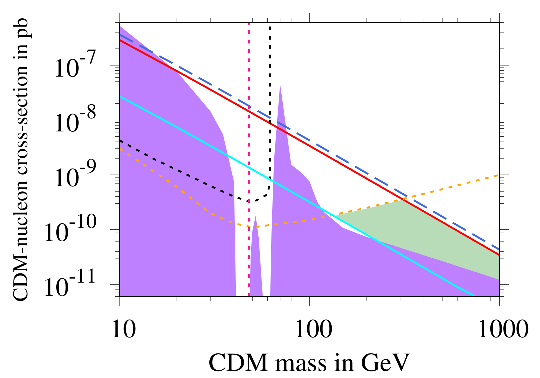
Figure 5: The CDM-nucleon cross-section versus the CDM mass for the CS model, for $\alpha=0.01$ (left) and $\alpha=0.1$ (right). Legends remain the same as in Fig. 4. Only the green shaded region is allowed.

A look at Fig. 4 should tell the reader how the constraints work. The left plot displays the allowed region for $d_{2}$, and the right one for $\delta_{2}$. The green shaded region is what ultimately remains allowed, after all the theoretical and experimental constraints are imposed. If $m_{\rm CDM}<m_{\chi}/2\approx 48$ GeV, $\chi$ decays almost entirely to the CDM pair, and each of the models fail to explain the CMS signal strength, so that region is ruled out, shown by a vertical dashed line in the subsequent plots. For $m_{\rm CDM}>m_{\chi}$, the overclosure bound is almost entirely controlled by the CDM pair annihilation to $\chi\chi$. Below this, the CDM pair can annihilate to $b\bar{b}$ (through the doublet component of $\chi$), $\gamma\gamma$, or $gg$ (through the effective operators). All these channels have been taken into account for our analysis.

The salient features of these plots are:

• The mixed quartic $\delta_{2}$ is much more tightly constrained from the pure singlet quartic $d_{2}$. This is because of its role in the scalar mass matrix as well as the RG equations. However, the nature of the two plots is very similar.

• For low values of $\alpha$, the parameter space ruled out by the direct detection limit and that ruled out from the invisible Higgs decay are competitive. However, triviality and scattering unitarity (which essentially put some upper bounds on the couplings) rule out a significant amount of parameter space that is still allowed by direct detection; only a narrow slice is ruled out by the stability condition. Altogether, these constraints rule out a large chunk of the parameter space, particularly for $m_{S_{2}}>200$ GeV. Again, this depends on the scale $\Lambda$ where the CS model is taken over by some ultraviolet-complete theory. The plots were drawn with $\Lambda=100$ TeV; if it is higher, the green region will be even more squeezed.

• The single narrow resonance region for the RS model now expands to two closely lying such regions. The lower mass one comes from the apparent stability of $\chi$, and the higher mass one from that of $h$.

• At the same time, the CDM mass below 48 GeV is ruled out from the CMS signal; this is shown by a vertical dashed line in Fig. 4 and all subsequent figures. In this region, $\chi$ decays almost entirely to a CDM pair, and the branching ratio to diphoton suffers a huge suppression by several orders of magnitude, incompatible with the signal strength.

In Fig. 4, we show identical plots but for $\alpha=0.1$. While the qualitative features remain similar to Fig. 4, there are two important changes. First, for the $\delta_{2}$-plot, the direct detection limit remains more or less the same, but the stability line has moved up, indicating a tighter lower limit. The close pair of lines, marking scattering unitarity and triviality bounds, have also moved up, relaxing the corresponding bounds. For the $d_{2}$-plot, these lines do not change, which can qualitatively be understood from the RG equations. What changes significantly is the direct detection bound, and as a result, it starts to cut in the theoretical constraints for lower values of $m_{S_{2}}$, approximately $m_{S_{2}}<200$ GeV. Second, the resonance regions have become wider, which can be explained easily from the $\alpha$-dependence of the couplings between physical scalars.

One can translate these bounds directly to the CDM-nucleon scattering cross-section limits, which is shown in Fig. 5, for both $\alpha=0.01$ and $\alpha=0.1$.

3.2 The RSF model

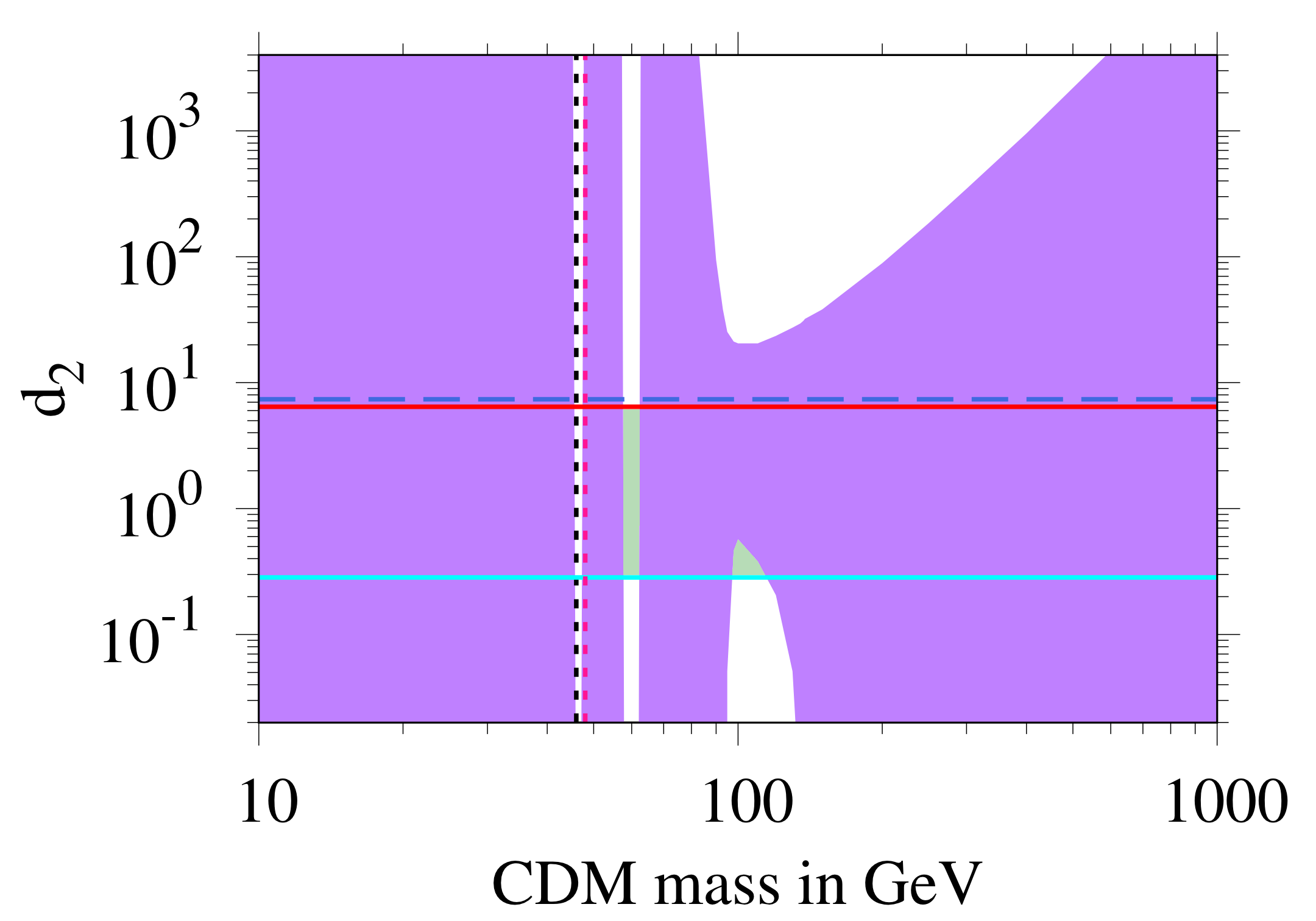
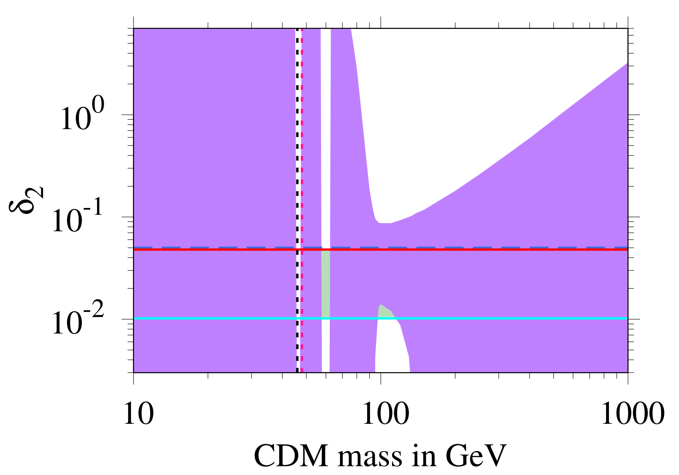
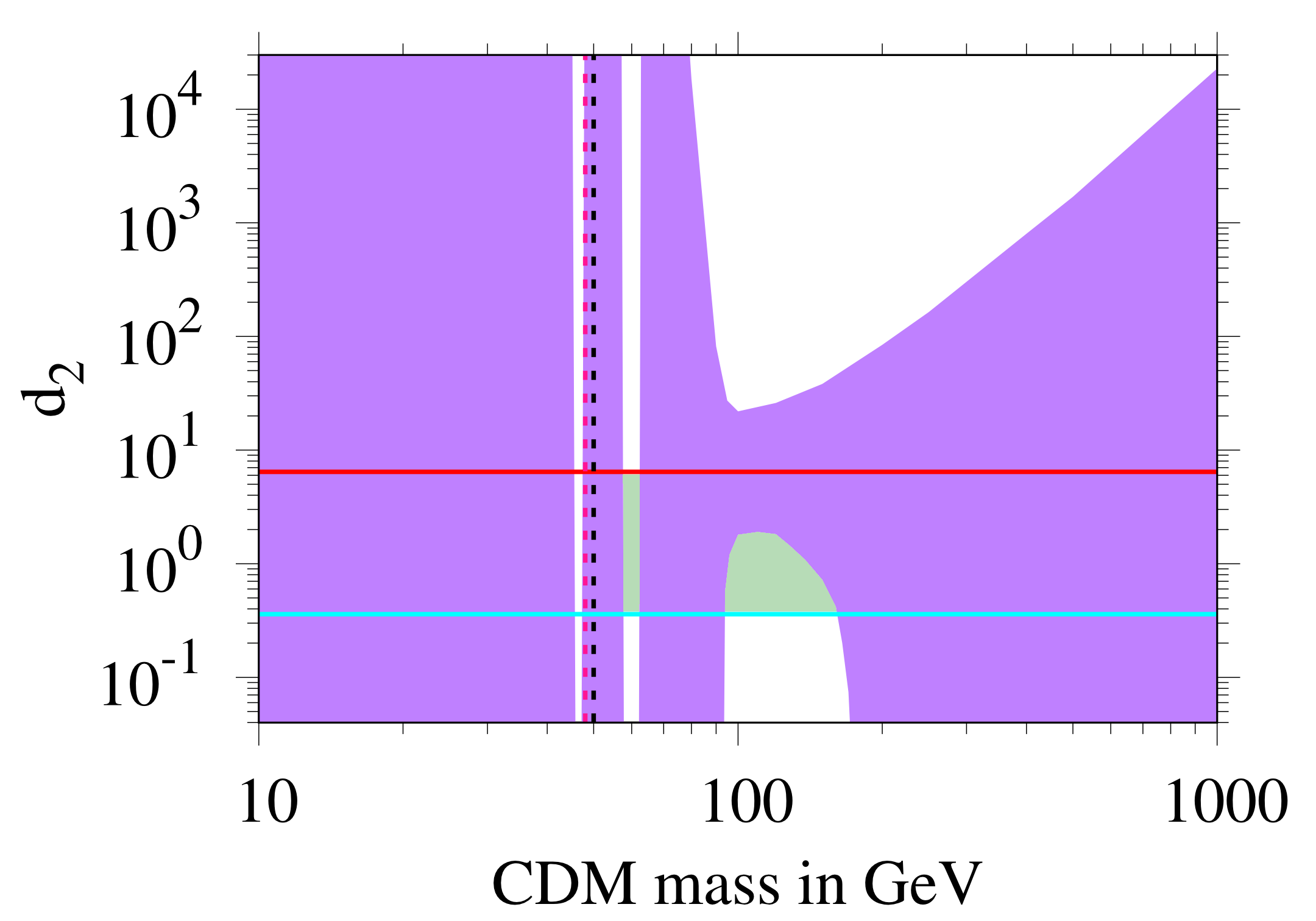
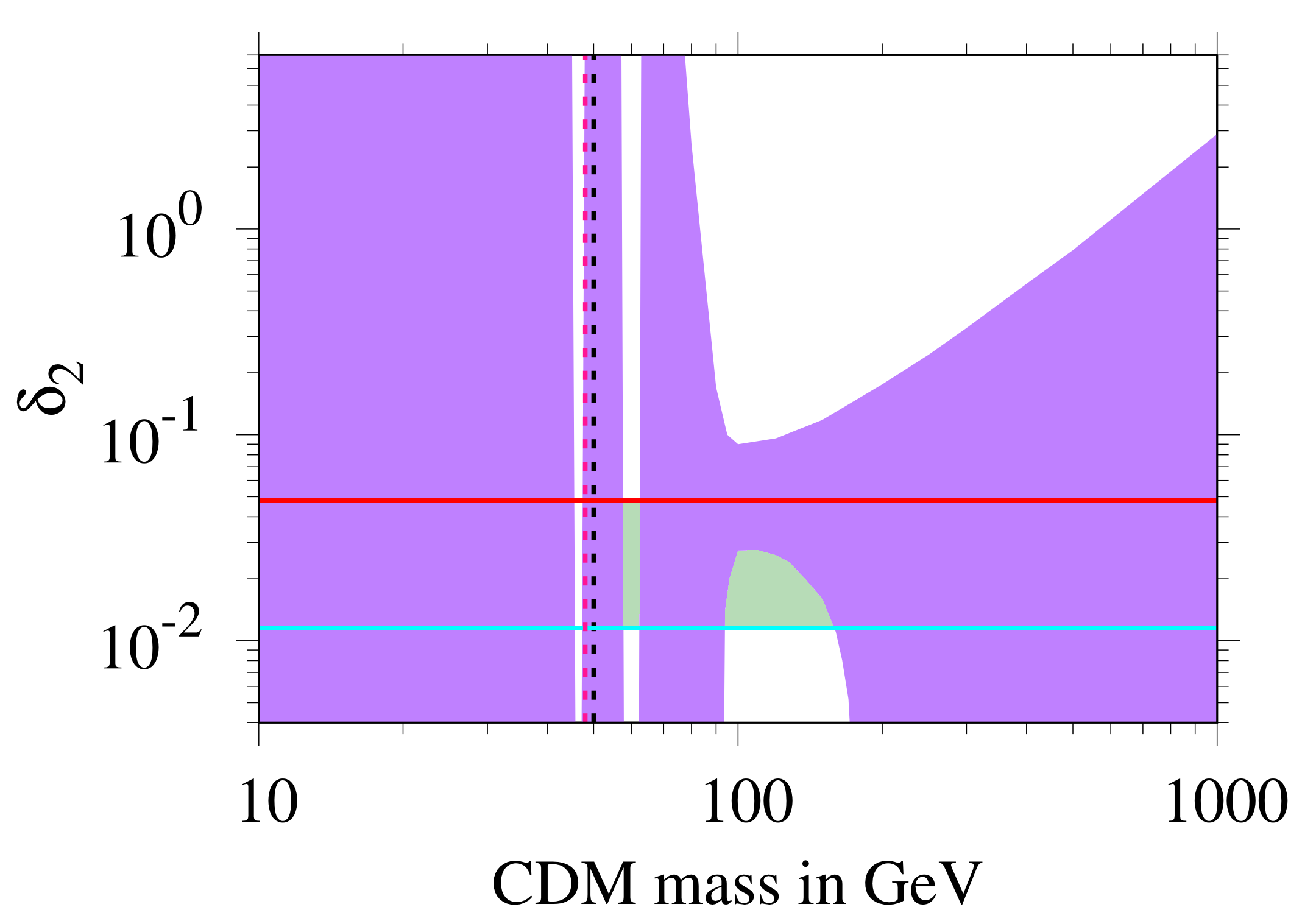
Figure 6: The allowed parameter space for the RSF model for $\alpha=0.05$ and Yukawa coupling $Y=0.7$. The fermion $\psi$ is the CDM candidate. The purple region is excluded from overclosure, the portion above the red and blue horizontal lines (which are overlapping in these plots) are excluded from scattering unitarity and triviality bounds respectively, and the portion below the horizontal cyan line near the bottom is excluded from the stability of the potential (which becomes unbounded from below). The region left to the short-dashed black line is excluded from the invisible decay of the Higgs, and that left to the vertical dashed line at 48 GeV from the CMS signal strength. Only the green shaded region remains allowed. The entire region is allowed from the direct detection bounds.

Figure 7: The same as Fig. 7 but with $Y=0.85$. All other legends remain the same.

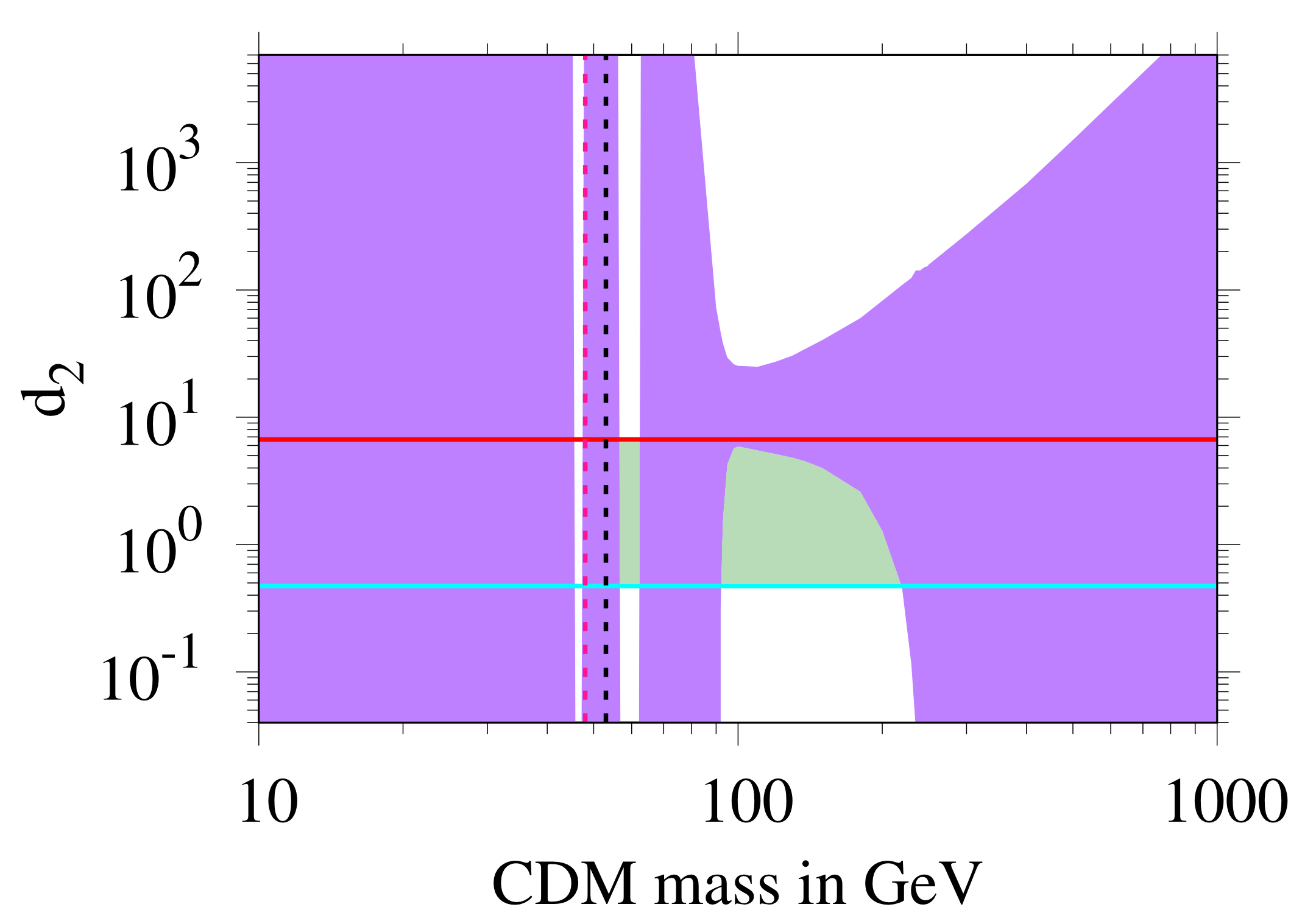
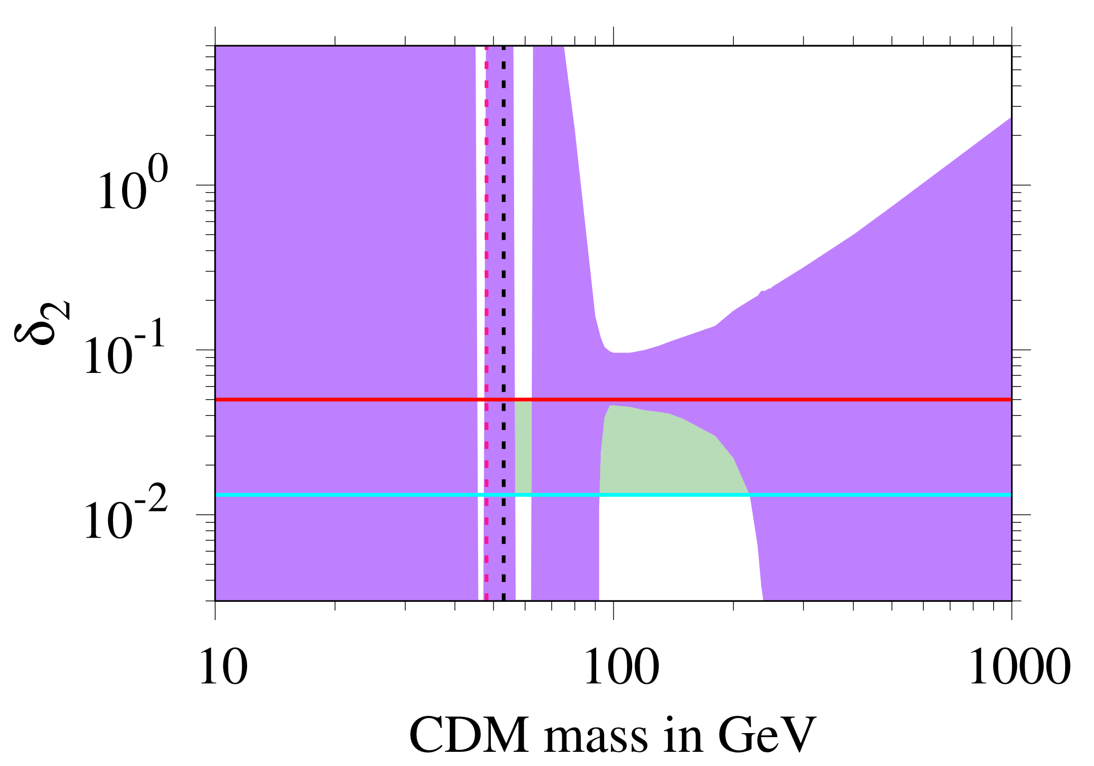
Figure 8: The same as Fig. 7 but with $Y=1$. All other legends remain the same.

The allowed parameter space for the RSF model is shown in Figs. 7, 7, and 8. The fermion $\psi$ is the CDM candidate, and couples only to the real singlet $S$. Thus, for a large enough Yukawa coupling $Y$ between $S$ and $\psi$, or $h_{Q}$ between $S$ and $Q$ (in Subclass (a) models) the potential runs the risk of being unbounded from below at a high scale. In Figs. 7-8, we have also delineated the region where such a catastrophe takes place (the lower part of the horizontal cyan line). The instability threshold is taken, again, to be at 100 TeV or more, i.e., some other new physics comes into play at that scale to make the potential stable. While the entire region showed in these figures is allowed from the direct detection limits, one may note the power of the triviality and stability constraints, which ultimately leaves only a narrow region around 150 GeV as allowed. The allowed region expands for larger values of $Y$, as the overclosure bound starts shrinking.

For Figs. 7-8, the mixing angle $\alpha$ is fixed at $0.05$. For higher values of $\alpha$, $\psi$ couples with $h$ more strongly and hence direct detection constraints tend to rule out more of the allowed parameter space shown here. For even smaller values of $\alpha$, resonance regions no longer exist. It is also easy to understand why the constraint from the invisible decay of the Higgs is a vertical line. The invisible decay width depends on the CDM mass, $\alpha$, and $Y$, but here $\alpha$ and $Y$ are fixed, so the only dependence is on $m_{\rm CDM}$.

The window near $m_{\rm CDM}\sim 150$ GeV, in Figs. 7-8, is interesting. Let us see what happens when we keep $m_{\rm CDM}$ fixed in that region but increase $d_{2}$ or $\delta_{2}$. Such a shift decreases $s_{1}$, the VEV of $S$. This increases the relic density to such a point as to hit the overclosure bound, so the region becomes disallowed and the neck begins. If we continue increasing $d_{2}$ or $\delta_{2}$, the relic density starts decreasing after a point (e.g., one may look at Fig. 1 to see how the annihilation cross-section changes, moving from right to left), and the parameter space again opens up, terminating the neck.

  

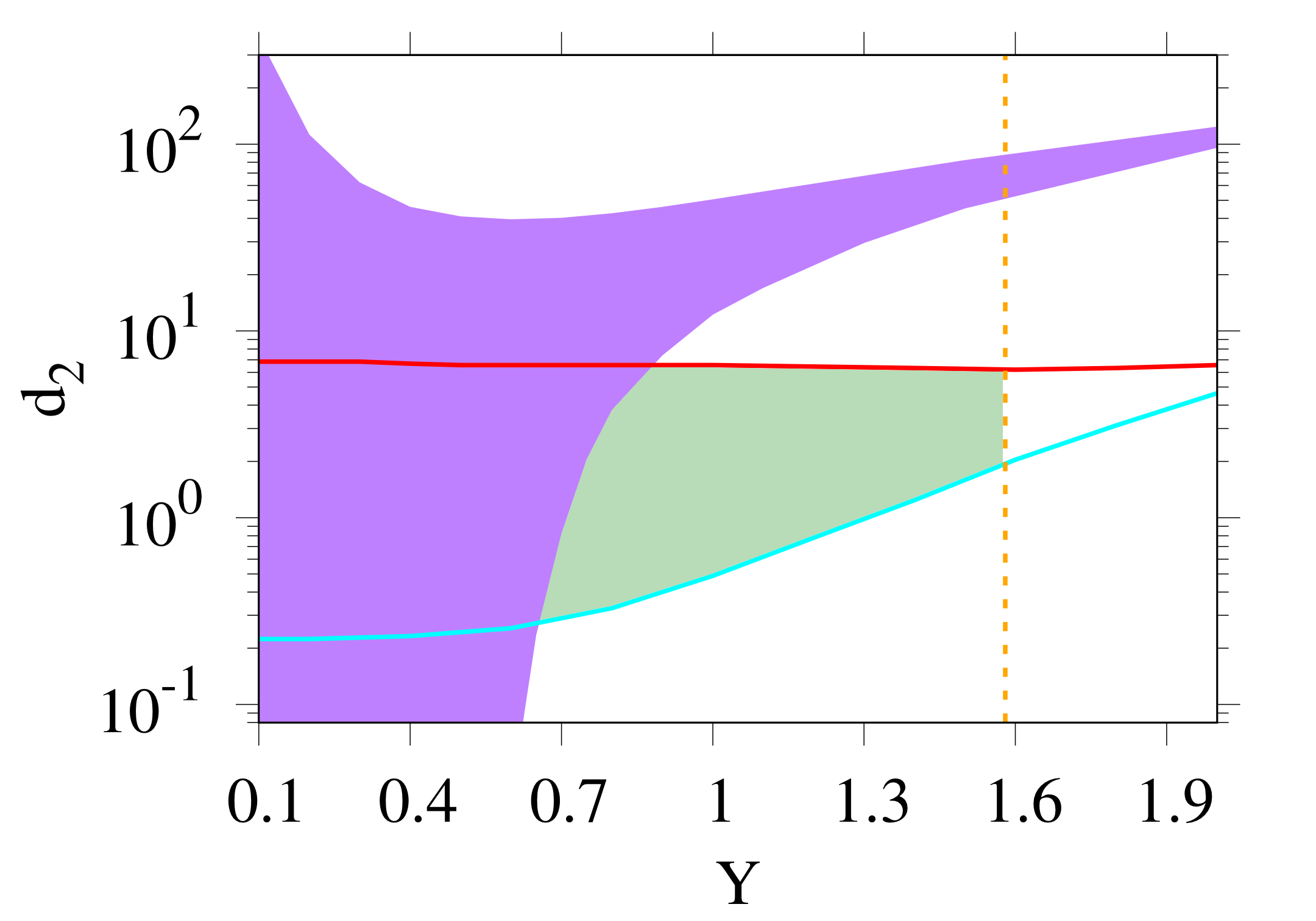
Figure 9: The allowed region for the RSF model, with $\alpha=0.05$ and $m_{\rm CDM}=100$ GeV. For details, see text. The region below the red horizontal line, above the cyan line, right to the overclosure patch, and left to the dashed orange vertical line, is allowed.

Let us also display the interdependence of the couplings $d_{2}$, $\delta_{2}$, and $Y$ in Fig. 9. Technically, this should depend on $h_{Q}$ too, but we have used a fixed value of the coupling. We kept the mixing angle at $\alpha=0.05$ and changed the scalar VEV $s_{1}$, which in turn controls $d_{2}$ and $\delta_{2}$. Apart from the shaded overclosure region, there are three lines in each plot. The vertical line at the right is the bound from direct detection; as the CDM mass is kept fixed at 100 GeV, the limit depends only on $Y$, and not on the scalar quartics. The region above the almost horizontal red line is ruled out because the couplings blow up before 100 TeV. Large values of $Y$ can delay the onset of the Landau pole; that is why the line veers slightly upwards for large $Y$ (although that region is ruled out from direct detection). The region below the cyan line is ruled out because the potential, at least at the tree-level, becomes unstable there. Only the island within these three lines and the overclosure region remains allowed.

3.3 The CSF-2 model

The CSF-1 model, with the fermion being the sole dark matter candidate, is qualitatively very similar to the RSF model, even more so if the second singlet scalar is heavy. We, thus, do not explicitly show the features, and rather concentrate on CSF-2. As both the scalar $S_{2}$ and the fermion $\psi$ can be CDM candidates, we denote their masses by $m^{S}_{\rm CDM}$ and $m^{F}_{\rm CDM}$ respectively.

   

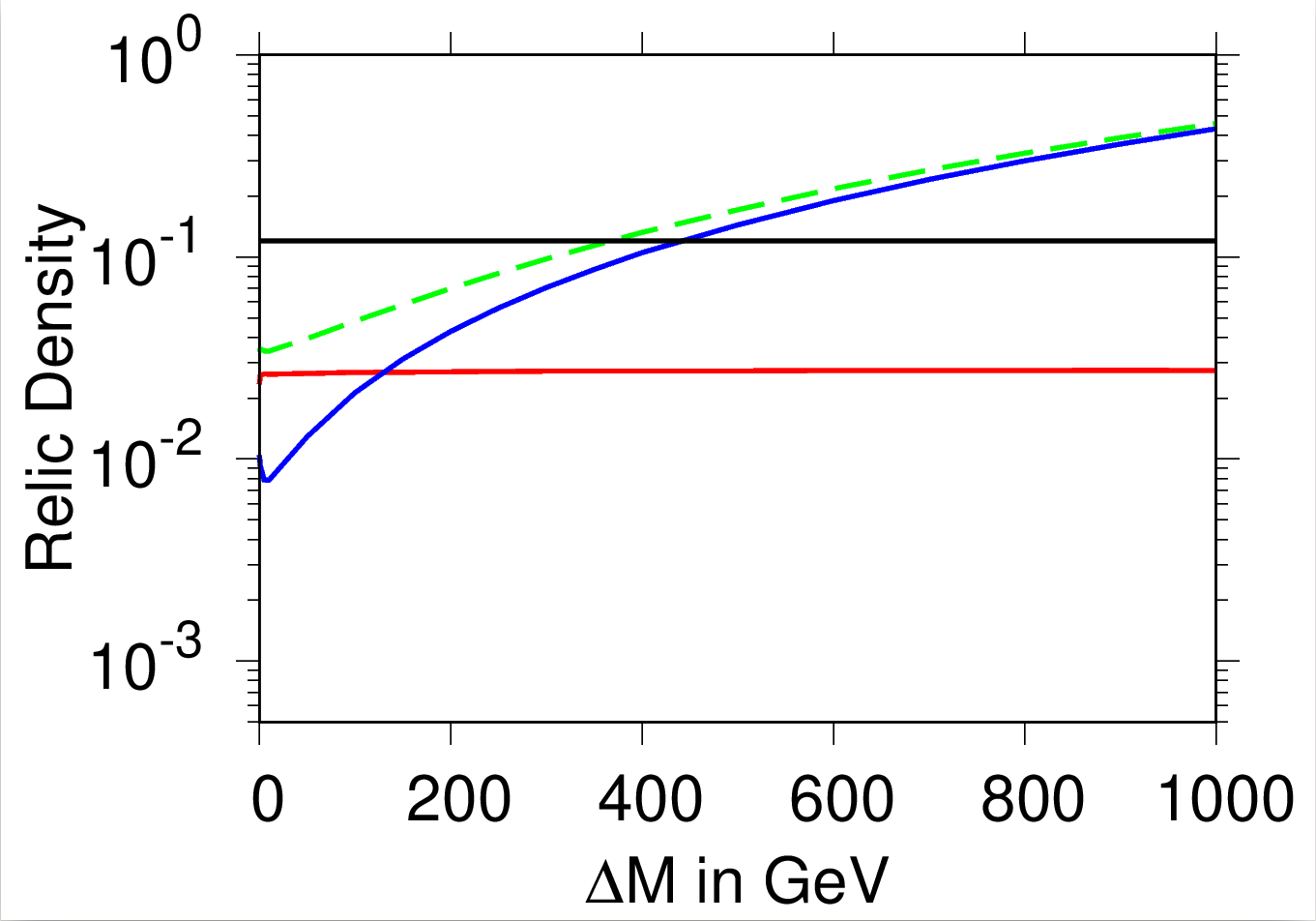
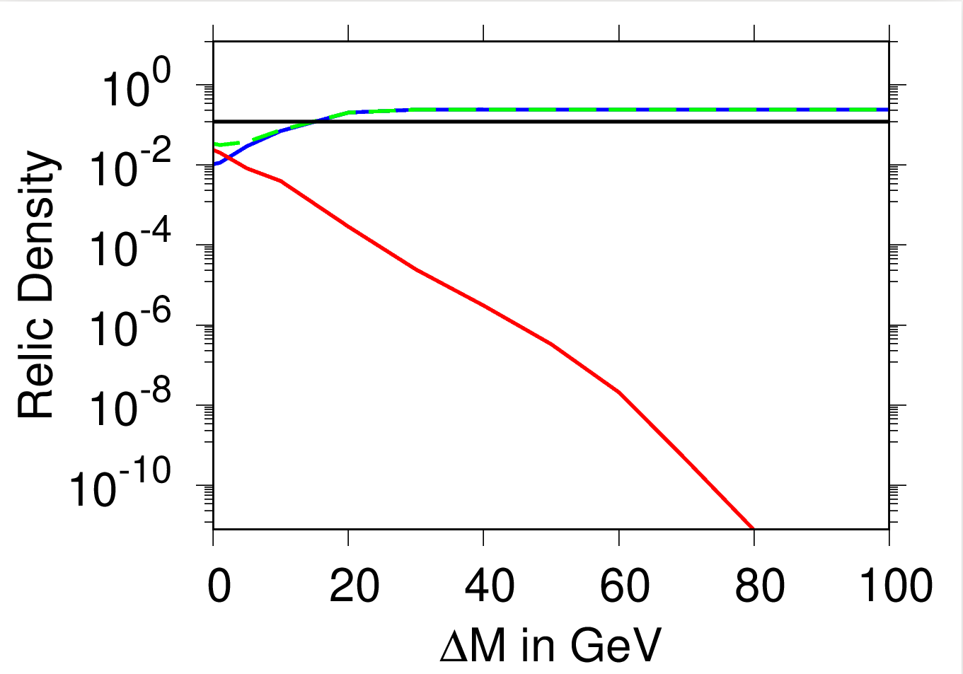
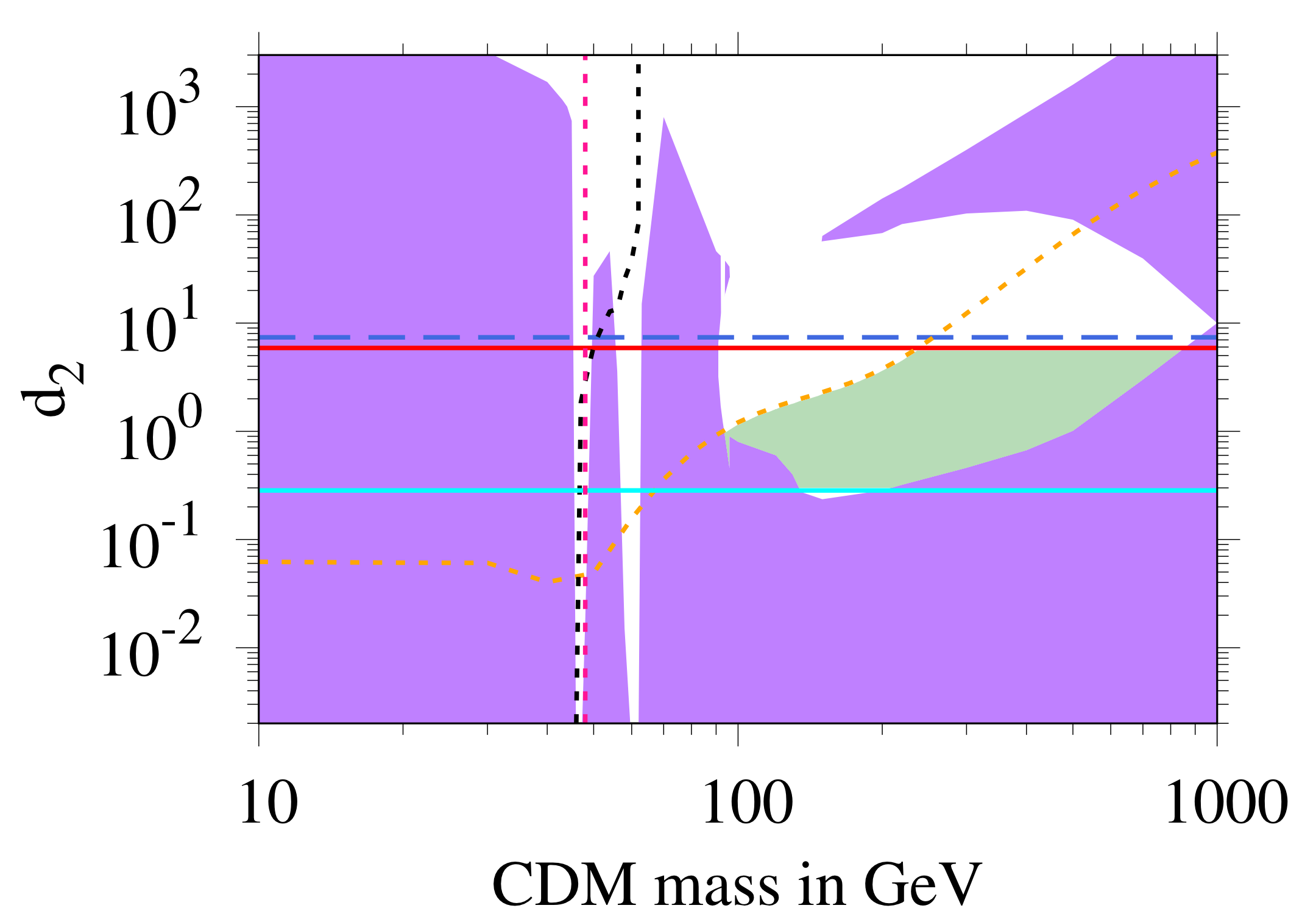
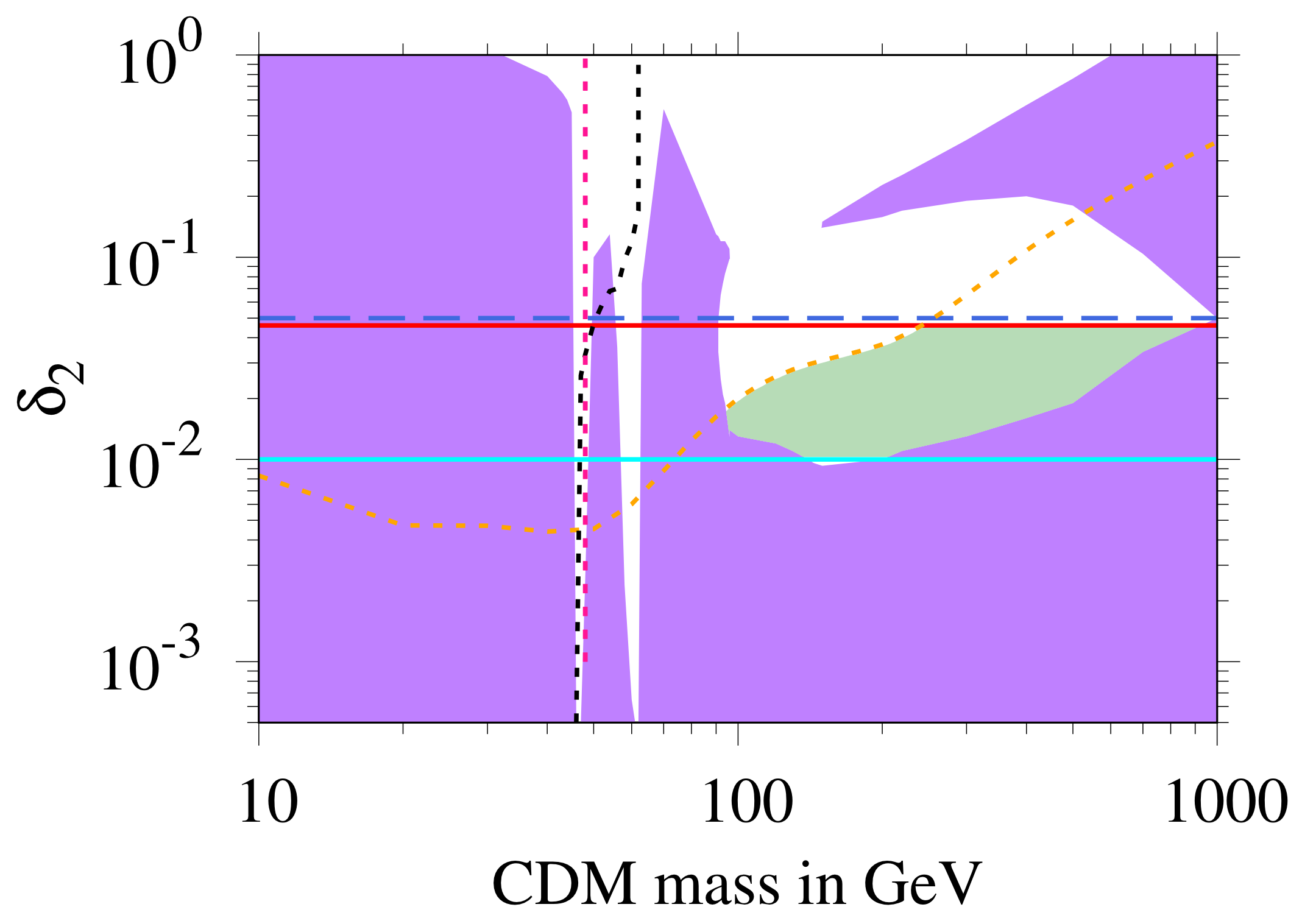
Figure 10: The composition of the CDM in the CSF-2 model, with the mass difference $\Delta M$ (in GeV) of the CDM components plotted against the relic density. The blue line corresponds to the contribution of $\psi$ and the red line to that of $S_{2}$, while the green line gives the combined contribution. Left: $m^{F}_{\rm CDM}>m^{S}_{\rm CDM}=100$ GeV. Right: $m^{S}_{\rm CDM}>m^{F}_{\rm CDM}=100$ GeV. For both the plots, the Yukawa coupling $Y=0.7$ and the singlet scalar VEV $s_{1}=100$ GeV. The relic density limit $\Omega h^{2}=0.12$ is also shown by the black horizontal line.

Figure 11: The allowed parameter space for the CSF-2 model for $\alpha=0.05$ and Yukawa coupling $Y=0.7$. The legends are identical with that of Fig. 7, apart from the dashed orange line, the region above which is excluded from the direct detection experiments. For more explanation, see text.

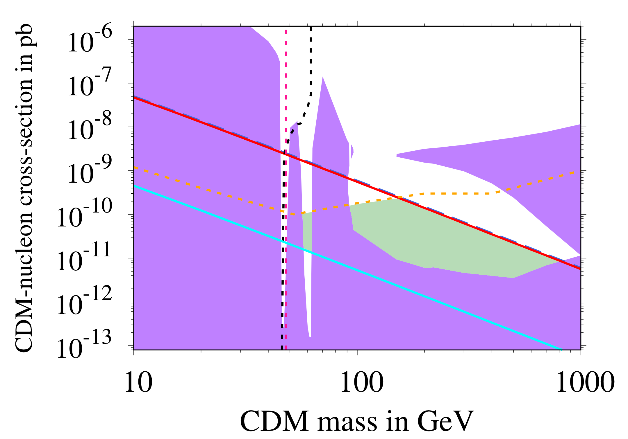
Figure 12: The CDM-nucleon cross-section versus the CDM mass for the CSF-2 model for $\alpha=0.05$ and Yukawa coupling $Y=0.7$. Legends remain the same as in Fig. 11. Only the green shaded region is allowed.

  

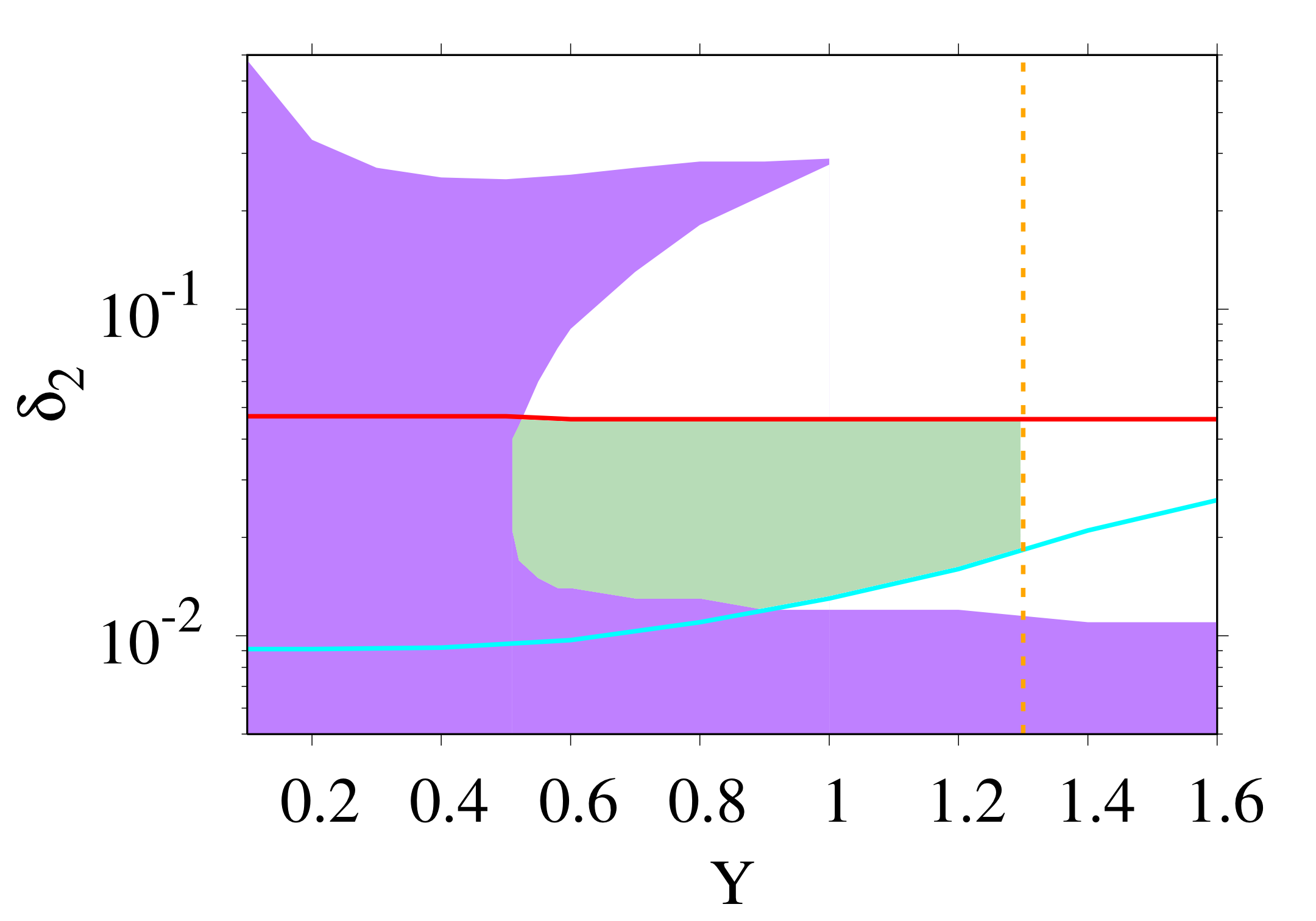
Figure 13: The allowed region for the CSF-2 model, with $\alpha=0.05$ and $m^{F}_{\rm CDM}=m^{S}_{\rm CDM}+200$ MeV. The region below the red horizontal line, above the cyan line, right to the overclosure patch, and left to the vertical line, is allowed.

With these two possible candidates, there can be interconversions, $\bar{\psi}\psi\leftrightarrow S_{2}S_{2}$, and the standard annihilations to bosonic and fermionic final states. The composition of the dark matter is shown in Fig. 11, with $Y=0.7$ and scalar VEV $s_{1}=100$ GeV. In the left plot, we take $m^{F}_{\rm CDM}>m^{S}_{\rm CDM}$, and in the right plot, $m^{F}_{\rm CDM}<m^{S}_{\rm CDM}$, the mass of the lighter one being fixed at 100 GeV. Note that if $m^{S}_{\rm CDM}>m^{F}_{\rm CDM}$, it quickly saturates the $\Omega h^{2}=0.12$ limit. If $m^{F}_{\rm CDM}$ is heavier of the two, its contribution slowly rises with the mass difference $\Delta M$, and hits the relic density limit at $\Delta M\approx 450$ GeV. One may note that for the left panel of Fig. 11, both $S_{2}$ and $\psi$ can be CDM components, while for the right panel, $S_{2}$ ceases to be a CDM component if the channel $S_{2}\to\psi\bar{\psi}$ opens up. However, the overclosure bound is reached much before that.

The allowed parameter space for the CSF-2 model is shown in Fig. 11, with $m^{F}_{\rm CDM}=m^{S}_{\rm CDM}+200$ MeV, $\alpha=0.05$ and $Y=0.7$. One finds that the plots display traits similar to both CS and RSF models, as expected. For example, the line showing the invisible decay constraint starts out vertically for small $d_{2}$ or $\delta_{2}$, like the RSF model, and then shows a rightward shift as found for the CS model. One may note the important role the triviality and unitarity lines play; they cut out a significant portion of the otherwise allowed parameter space.

Fig. 12 shows the allowed region for the CDM-nucleon scattering cross-section, analogous to Fig. 5. Fig. 13, similarly, shows the allowed region for the parameters of the potential, analogous to Fig. 9.

4 Conclusion

In this paper, we have studied the parameter space for several extensions of the SM that provide one or more cold dark matter candidates as well as a scalar at 96 GeV. The existence of the latter was only hinted by the CMS Collaboration, but if tagged with a CDM model, this provides further constraints on the parameter space, by reducing the number of free parameters in the Lagrangian.

We analysed the parameter space of three models: (i) SM plus a complex scalar singlet (CS), with one of the scalars being the CDM, and the other giving rise to the 96 GeV resonance after mixing with the SM doublet; (ii) SM plus a real scalar singlet and a singlet vectorial fermion (RSF), with the fermion being the dark matter; and (iii) CS plus a singlet vectorial fermion (CSF), with both fermion and scalar being dark matter candidates. The theoretical constraints that were taken into account includes the stability of the potential (both triviality and boundedness), the scattering unitarity (although it hardly differs from the triviality constraints), and the oblique parameters, the effect of the latter being negligible. The experimental constraints include those coming from the direct detection of dark matter, the overclosure bound on the relic density ($\Omega h^{2}<0.12$), and the invisible decay width of the Higgs boson. We have assumed a thermalised nonrelativistic dark matter and used micrOMEGAs v5.0.8 to generate the relic density.

At the same time, we have shown how the diphoton signal can be explained, either in some ultraviolet-complete theory, or in some effective theory framework. Combined with the CDM models, they provide a number of significant constraints on the parameter space of such models. In this paper, we collect and display for the first time, all such possible theoretical and experimental constraints on the allowed parameter space of these three models, extending the CDM mass to 1 TeV. Several interesting features emerge from the analysis, and they have been displayed in the previous section. One may enlist them once again here:

1. The triviality/unitarity constraints play a vital role in restricting the allowed parameter space for the CS and the CSF-2 models. In fact, the parameter space gets further squeezed if we assume the possible onset of a new physics at higher than 100 TeV. The severity of their effect depends on the singlet-doublet mixing angle $\alpha$. If $\alpha$ is small enough, one finds that these constraints are always more powerful than those coming from direct detection. With larger values of $\alpha$, they become comparable. On the other hand, the constraint arising out of the requirement of stability of the potential is significant only in the RSF model, or for larger values of $\alpha$.

2. The CS and the CSF-2 models allow two narrow resonance regions, at approximately $m_{h}/2$ and $m_{\chi}/2$, and they become wider as the mixing angle increases. Thus, one may still have a sub-100 GeV scalar dark matter, which is not overly fine-tuned. However, $m_{\rm CDM}<m_{\chi}/2$ is ruled out from the CMS signal strength.

3. The RSF model is much more tightly constrained than its CS or CSF counterparts. A large part of the parameter space allowed from the relic density bound is ruled out by triviality and unitarity limits. However, there exists a narrow window, which is one of the novel findings of this paper, and whose position depends on the singlet scalar VEV, while the width depends on the Yukawa coupling $Y$. The ruled-out neck region, just above the window, appears because of the destructive interference between the $s$- and $t$-channel annihilation amplitudes, although a significant part of this window is truncated from the stability of potential.

While such a study might be interesting to the model builders as well as those looking for collider signatures of beyond-SM physics, one must be cautious in applying these bounds. The parameter space, even after allowing for the 96 GeV scalar, is complicated enough, and we have refrained from doing a complete scan over all the parameters. The allowed regions will shift for different values of the scalar VEV $s_{1}$, the CDM mass, or the splitting between the two CDM candidates for the CSF-2 model. However, we expect the general trends to remain qualitatively similar.

Acknowledgement: AK acknowledges the Science and Engineering Research Board, Government of India, for support through the Grant EMR/2016/001306 and the DIA fellowship.

References

- [1] M. Tanabashi et al. [Particle Data Group], Phys. Rev. D 98, no. 3, 030001 (2018).
-
[2]
See, for example, G. Bertone, Particle Dark Matter (Cambridge University Press, 2010);
M. Cirelli, N. Fornengo and A. Strumia, Nucl. Phys. B 753, 178 (2006) [hep-ph/0512090];
J. L. Feng, Ann. Rev. Astron. Astrophys. 48, 495 (2010) [arXiv:1003.0904 [astro-ph.CO]];
M. Drees and G. Gerbier, in Review of Particle Physics, Phys. Rev. D 98, no. 3, 030001 (2018). - [3] G. Arcadi, A. Djouadi and M. Raidal, Phys. Rept. 842, 1 (2020) arXiv:1903.03616 [hep-ph].
- [4] G. Arcadi, M. Dutra, P. Ghosh, M. Lindner, Y. Mambrini, M. Pierre, S. Profumo and F. S. Queiroz, Eur. Phys. J. C 78, no. 3, 203 (2018) [arXiv:1703.07364 [hep-ph]].
- [5] A. M. Sirunyan et al. [CMS Collaboration], Phys. Lett. B 793, 320 (2019) [arXiv:1811.08459 [hep-ex]].
- [6] J. Cao, X. Guo, Y. He, P. Wu and Y. Zhang, Phys. Rev. D 95, no. 11, 116001 (2017) [arXiv:1612.08522 [hep-ph]].
- [7] L. Liu, H. Qiao, K. Wang and J. Zhu, Chin. Phys. C 43, no. 2, 023104 (2019) [arXiv:1812.00107 [hep-ph]].
- [8] S. Heinemeyer and T. Stefaniak, PoS CHARGED 2018, 016 (2019) [arXiv:1812.05864 [hep-ph]].
- [9] T. Biekötter, M. Chakraborti and S. Heinemeyer, PoS CORFU 2018, 015 (2019) arXiv:1905.03280 [hep-ph]; T. Biekötter, M. Chakraborti and S. Heinemeyer, arXiv:2002.06904 [hep-ph].
- [10] K. Choi, S. H. Im, K. S. Jeong and C. B. Park, arXiv:1906.03389 [hep-ph].
- [11] J. M. Cline and T. Toma, Phys. Rev. D 100, no. 3, 035023 (2019) arXiv:1906.02175 [hep-ph].
- [12] M. Gonderinger, H. Lim and M. J. Ramsey-Musolf, Phys. Rev. D 86, 043511 (2012) [arXiv:1202.1316 [hep-ph]].
- [13] E. Gabrielli, M. Heikinheimo, K. Kannike, A. Racioppi, M. Raidal and C. Spethmann, Phys. Rev. D 89, no. 1, 015017 (2014) [arXiv:1309.6632 [hep-ph]].
- [14] K. Huitu, N. Koivunen, O. Lebedev, S. Mondal and T. Toma, Phys. Rev. D 100, no. 1, 015009 (2019) [arXiv:1812.05952 [hep-ph]].
- [15] K. S. Babu and E. Ma, Int. J. Mod. Phys. A 23, 1813 (2008) [arXiv:0708.3790 [hep-ph]].
- [16] Y. G. Kim, K. Y. Lee and S. Shin, JHEP 0805, 100 (2008) [arXiv:0803.2932 [hep-ph]].
- [17] S. Baek, P. Ko and W. I. Park, JHEP 1202, 047 (2012) [arXiv:1112.1847 [hep-ph]].
- [18] M. Fairbairn and R. Hogan, JHEP 1309, 022 (2013) [arXiv:1305.3452 [hep-ph]].
- [19] S. Matsumoto, S. Mukhopadhyay and Y. L. S. Tsai, JHEP 1410, 155 (2014) [arXiv:1407.1859 [hep-ph]].
- [20] A. Dutta Banik, A. K. Saha and A. Sil, Phys. Rev. D 98, no. 7, 075013 (2018) [arXiv:1806.08080 [hep-ph]].
- [21] S. Bhattacharya, A. Drozd, B. Grzadkowski and J. Wudka, JHEP 1310, 158 (2013) [arXiv:1309.2986 [hep-ph]].
- [22] S. Bhattacharya, A. Drozd, B. Grzadkowski and J. Wudka, Acta Phys. Polon. B 44, 2373 (2013) [arXiv:1310.7901 [hep-ph]].
- [23] S. Esch, M. Klasen and C. E. Yaguna, JHEP 1409, 108 (2014) [arXiv:1406.0617 [hep-ph]].
- [24] A. Dutta Banik, M. Pandey, D. Majumdar and A. Biswas, Eur. Phys. J. C 77, no. 10, 657 (2017) [arXiv:1612.08621 [hep-ph]].
- [25] S. Peyman Zakeri, S. Mohammad Moosavi Nejad, M. Zakeri and S. Yaser Ayazi, Chin. Phys. C 42, no. 7, 073101 (2018) [arXiv:1801.09115 [hep-ph]].
- [26] N. Bernal, D. Restrepo, C. Yaguna and . Zapata, Phys. Rev. D 99, no. 1, 015038 (2019) [arXiv:1808.03352 [hep-ph]].
-
[27]
A. Falkowski, O. Slone and T. Volansky,
JHEP 1602, 152 (2016)
[arXiv:1512.05777 [hep-ph]];
D. Buttazzo, A. Greljo and D. Marzocca, Eur. Phys. J. C 76, no. 3, 116 (2016) [arXiv:1512.04929 [hep-ph]];
S. Di Chiara, L. Marzola and M. Raidal, Phys. Rev. D 93, no. 9, 095018 (2016) [arXiv:1512.04939 [hep-ph]];
A. Angelescu, A. Djouadi and G. Moreau, Phys. Lett. B 756, 126 (2016) [arXiv:1512.04921 [hep-ph]]. -
[28]
Y. Mambrini, G. Arcadi and A. Djouadi,
Phys. Lett. B 755, 426 (2016)
[arXiv:1512.04913 [hep-ph]];
M. Backovic, A. Mariotti and D. Redigolo, JHEP 1603, 157 (2016) [arXiv:1512.04917 [hep-ph]]. - [29] M. D. Goodsell and F. Staub, Eur. Phys. J. C 78, no. 8, 649 (2018) [arXiv:1805.07306 [hep-ph]].
- [30] M. Flechl [CMS Collaboration], arXiv:1905.07150 [hep-ex].
- [31] D. S. Akerib et al. [LUX Collaboration], Phys. Rev. Lett. 118, no. 2, 021303 (2017) [arXiv:1608.07648 [astro-ph.CO]].
- [32] X. Cui et al. [PandaX-II Collaboration], Phys. Rev. Lett. 119, no. 18, 181302 (2017) [arXiv:1708.06917 [astro-ph.CO]].
- [33] E. Aprile et al. [XENON Collaboration], Phys. Rev. Lett. 119, no. 18, 181301 (2017) [arXiv:1705.06655 [astro-ph.CO]].
- [34] E. Aprile et al. [XENON Collaboration], Phys. Rev. Lett. 121, no. 11, 111302 (2018) [arXiv:1805.12562 [astro-ph.CO]].
- [35] L. Feng, S. Profumo and L. Ubaldi, JHEP 1503, 045 (2015) [arXiv:1412.1105 [hep-ph]].
- [36] M. Cirelli, N. Fornengo and A. Strumia, Nucl. Phys. B 753, 178 (2006) [hep-ph/0512090].
- [37] J. Herrero-Garcia, E. Molinaro and M. A. Schmidt, Eur. Phys. J. C 78, no. 6, 471 (2018) [arXiv:1803.05660 [hep-ph]].
- [38] P. Athron et al. [GAMBIT Collaboration], Eur. Phys. J. C 77, no. 8, 568 (2017) [arXiv:1705.07931 [hep-ph]].
- [39] J. Quilis, PoS EPS -HEP2017, 081 (2017) [arXiv:1710.08723 [hep-ph]].
- [40] P. Athron, J. M. Cornell, F. Kahlhoefer, J. Mckay, P. Scott and S. Wild, Eur. Phys. J. C 78, no. 10, 830 (2018) [arXiv:1806.11281 [hep-ph]].
-
[41]
W. J. Stirling, private communication, also see
http://www.hep.ph.ic.ac.uk/~wstirlin/plots/plots.html
- [42] V. Barger, P. Langacker, M. McCaskey, M. Ramsey-Musolf and G. Shaughnessy, Phys. Rev. D 79, 015018 (2009) [arXiv:0811.0393 [hep-ph]].
- [43] M. E. Machacek and M. T. Vaughn, Nucl. Phys. B 222, 83 (1983).
- [44] G. Belanger, F. Boudjema, A. Goudelis, A. Pukhov and B. Zaldivar, Comput. Phys. Commun. 231, 173 (2018) [arXiv:1801.03509 [hep-ph]].
-
[45]
F. Staub,
Adv. High Energy Phys. 2015, 840780 (2015)
[arXiv:1503.04200 [hep-ph]];
F. Staub, Comput. Phys. Commun. 185, 1773 (2014) [arXiv:1309.7223 [hep-ph]].