A phenomenological investigation of the integral and the differential versions of the $Kimber$-$Martin$-$Ryskin$ $unintegrated$ parton distribution functions using two different constraints and the $MMHT2014$ $PDF$

Abstract

We previously investigated the compatibility of the $Kimber$-$Martin$-$Ryskin$ ($KMR$) $unintegrated$ parton distribution functions ($UPDF$) with the experimental data on the proton (longitudinal) structure functions ($PSF$ ($PLSF$)). Recently $Golec-Biernat$ and $Stasto$ ($GBS$) demonstrated that the differential version of $KMR$ prescription and the implementations of angular (strong) ordering ($AOC$ ($SOC$)) constraints, cause the negative-discontinuous $UPDF$ with the ordinary parton distribution functions ($PDF$) as the input, which leads to a sizable effect on the calculation of $PSF$. In the present work, we use the new $MMHT2014$-$LO$-$PDF$ as the input and focus on the $UPDF$ behaviors as was raised by $GBS$. The resulting $PSF$ and $PLSF$ are compared with the $MSTW2008$-$LO$-$PDF$ and $MRST99$-$PDF$ and the 2014 data given by the $ZEUS$ and $H1$ collaborations. The calculated $PSF$ and $PLSF$ based on the integral prescription of the $KMR$-$UPDF$ with the $AOC$ and the ordinary $PDF$ as the input are reasonably consistent with the experimental data. Therefore, they are approximately independent to the $PDF$ (no need to impose cutoff on the $PDF$). At very small $x$ regions because of the excess of gluons in the $MMHT2014$-$LO$-$PDF$ and $MSTW2008$-$LO$-$PDF$, an increase in $PSF$ and $PLSF$ is achieved. Finally, according to the $GBS$ report the differential version by using the cutoff independent $PDF$ produces results far from the experimental data.

I Introduction

The parton distribution functions ($PDF$), $a(x,Q^{2})$ = $xq(x,Q^{2})$ and $xg(x,Q^{2})$, in which $x$ and $Q$ are the longitudinal momentum fraction and the factorization or hard scale, respectively, are the main phenomenological objects in the high energy collisions computations of particle physics. These $PDF$ usually can be extracted from the experimental data via the parametrization procedures which are constrained by the sum rules and a few theoretical assumptions. These functions which usually called $integrated$ parton distributions, satisfy the standard $Dokshitzer$-$Gribov$-$Lipatov$-$Altarelli$-$Parisi$ ($DGLAP$) evolution equations 1a ; 1b ; 1c ; 1d . The $DGLAP$ evolution equations are derived by integrating over the parton transverse momentum up to $k_{t}^{2}=Q^{2}$. Thus the usual $PDF$ are not the $k_{t}$-dependent distributions.

On the other hand, there exist plenty of experimental data on the various events, such as the exclusive and semi-inclusive processes in the high energy collisions in the $LHC$, which indicate the necessity for computation of the $k_{t}$-dependent parton distribution functions. These functions are $unintegrated$ over $k_{t}$ and are called the $unintegrated$ parton distribution functions ($UPDF$). The $UPDF$ are the two-scale dependent functions that can be generated via the $Ciafaloni$-$Catani$-$Fiorani$-$Marchesini$ ($CCFM$) formalism 5 ; 6 ; 7 ; 8 . Working in this framework is a hard and restrictive task. Also, there is not a complete quark version of the $CCFM$ formalism. Therefore, to overcome the complexity of the $CCFM$ equations and to calculate the $UPDF$, $Kimber$, $Martin$ and $Ryskin$ ($KMR$) 91 proposed a procedure which is based on the standard $DGLAP$ equations in the $LO$ approximation, along with a modification due to the strong ordering condition ($SOC$) in transverse momentum of the real parton emission, which comes from the coherence effect 92 . The prescription along with $SOC$ was further modified in the reference 9 due to the angular ordering condition ($AOC$), which is the key dynamical property of the $CCFM$ formalism (it is semi-$NLO$ formalism).

In our previous works 13 ; 14 ; 14p , to validate $KMR$ approach, we have utilized the $unintegrated$ parton distribution functions in the $KMR$ $k_{t}$-factorization procedure by using the set of $MRST99$ MRST and $MSTW2008$-$LO$ MSTW $PDF$ as the inputs to calculate the proton structure function and the proton longitudinal structure function. Also, we successfully used the $UPDF$ of the $KMR$ approach to calculate the inclusive production of the $W$ and $Z$ gauge vector bosons WZ ; z , the semi-$NLO$ production of Higgs bosons H and the production of forward-center and forward-forward di-jets di .

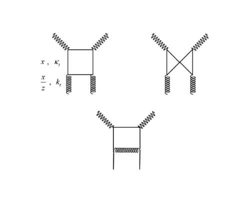
Figure 1: The diagrams contributing in the calculation of the structure functions $F_{2}(x,Q^{2})$, which comes from the $g\rightarrow q\overline{q}$ and $q\rightarrow qg$.

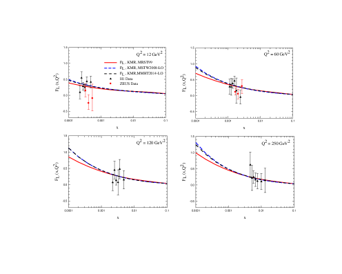
Figure 4: The proton longitudinal structure functions $F_{L}(x,Q^{2})$ based on the integral form of the $KMR$ approach with the $AOC$ constraint as a function of $x$ for various $Q^{2}$ values, by using the $MRST99$ MRST , the $MSTW2008$-$LO$ MSTW and the $MMHT2014$-$LO$ 22 as the inputs, are compared with the $ZEUS$ ZEUS and $H1$ H1 experimental data.

Recently $Golec-Biernat$ and $Stasto$ ($GBS$) GBS pointed out that different versions of $KMR$ prescriptions as well as implementations of angular ordering ($AOC$) and strong ordering ($SOC$) constraints, can cause negative and discontinuous $UPDF$ with the collinear global parton distribution functions ($PDF$) as the input that come from a global fit to data using the conventional collinear approximation, which in turn especially can cause a sizable effect on the calculation of proton structure functions. They showed that despite seemingly mathematical equivalence between the different versions of $KMR$ prescriptions with the same constraints, different results are obtained using the ordinary $PDF$ as the input (see the figure 1 of the reference GBS ). Also, they have shown that the integral form $KMR$-$UPDF$ by using the ordinary $PDF$ and the cutoff dependent $PDF$ as inputs, gives approximately the same results (see the figure 4 of the reference GBS ), in contrast to the differential form. They conclude that, this un-physical behavior happens in the differential form $KMR$ prescription (see the equation (10) of $GBS$, the references 9 ; Golec31 and the section $II$ of present report), otherwise one should impose cut off on the input $PDF$ . As it is stated in the reference watt2004 , the application of the integrated $PDF$ in the last evolution step should be generated through a new global fit to the data using the $k_{t}$-factorization procedures. This was estimated to lower the proton structure functions by 10 per cent watt2004 (if one ignores this $k_{t}$-factorization fitting).

In the present work, following our previous investigations, we intend to calculate the proton structure functions and the proton longitudinal structure functions by using the different versions of the $KMR$ $k_{t}$-factorization procedure 9 and taking into account the $PDF$ of $Martin$ et al. i.e., $MMHT2014$-$LO$ 22 as the input. The results of the integral version with $AOC$ are compared with our previous studies based on the $MRST99$ and $MSTW2008$-$LO$ input $PDF$ and the data given by the $ZEUS$ ZEUS and $H1$ H1 collaborations. In general, it is shown that our calculations are reasonably consistent with the experimental data and, by a good approximation, they are independent of the input $PDF$. It is also shown that the calculated proton structure function and the proton longitudinal structure function based on the integral prescription of the $KMR$-$UPDF$ with the $AOC$ constraint and the ordinary $PDF$ as the input are reasonably consistent with the experimental data. Therefore, they are approximately independent to the $PDF$ i.e. no need to impose cutoff on the $PDF$. However, at very small $x$ regions because of the excess of gluons in the input $PDF$ of the $MMHT2014$-$LO$ and $MSTW2008$-$LO$, a better agreement is achieved (see the panels $Q^{2}$=$12$ $GeV^{2}$). Finally, according to the $GBS$ report by considering the integral prescription of the $KMR$-$UPDF$ (see the figure 1 of the reference GBS and compare the solid curves of the left and right panels together) and the differential version of the $KMR$-$UPDF$, and using the cutoff independent $PDF$, we show the integral version with the $SOC$ constraint and the differential version produces results far from experimental data than the integral version with $AOC$ constraint especially as the hard scale is increased.

So the paper is organized as follows: in the section $II$ we give a brief review of the different versions of the $KMR$ approach 9 for the extraction of the $UPDF$ form, regarding the phenomenological $PDF$. The formulation of $F_{2}(x,Q^{2})$ and $F_{L}(x,Q^{2})$ based on the $k_{t}$-factorization approach are given in the section $III$. Finally, the section $IV$ is devoted to results, discussions, and conclusions.

II A brief review of the $KMR$ approach

The $KMR$ 9 approach was developed to calculate the $UPDF$, $f_{a}(x,k_{t}^{2},Q^{2})$, by using the given $PDF$, ($a(x,Q^{2})$ = $xq(x,Q^{2})$ and $xg(x,Q^{2})$), and the corresponding splitting functions $P_{aa^{\prime}}(x)$ at leading order ($LO$). This approach is the modification to the standard $DGLAP$ evolution equations by imposing the angular ordering constraint ($AOC$), which is the consequence of coherent gluon emissions (see below for the case of strong ordering constraint). The $KMR$ approach has two different versions that have a seemingly mathematical equivalence.
1. Integral form:
In integral form of the $KMR$ approach the separation of the real and virtual contributions in the $DGLAP$ evolution chain at the $LO$ level leads to the following forms for the quark and the gluon $UPDF$:

$$f_{q}(x,k_{t}^{2},Q^{2}) = T_{q}(k_{t},Q)\frac{\alpha_{s}({k_{t}}^{2})}{2\pi}$$ (1)

$$\times \int_{x}^{1-\Delta}dz\Bigg{[}P_{qq}(z)\frac{x}{z}\,q\left(\frac{x}{z},{k_{t}}^{2}\right)$$

$$+ P_{qg}(z)\frac{x}{z}\,g\left(\frac{x}{z},{k_{t}}^{2}\right)\Bigg{]},$$ (2)

$$f_{g}(x,k_{t}^{2},Q^{2}) = T_{g}(k_{t},Q)\frac{\alpha_{s}({k_{t}}^{2})}{2\pi}$$ (3)

$$\times \int_{x}^{1-\Delta}dz\Bigg{[}\sum_{q}P_{gq}(z)\frac{x}{z}\,q\left(\frac{x}{z},{k_{t}}^{2}\right)$$

$$+ P_{gg}(z)\frac{x}{z}\,g\left(\frac{x}{z},{k_{t}}^{2}\right)\Bigg{]},$$ (4)

respectively, while survival probability factor $T_{a}$ is evaluated from:

$$T_{a}(k_{t},Q) = \exp\Bigg{[}-\int_{k_{t}^{2}}^{Q^{2}}\frac{\alpha_{s}({k^{\prime}_{t}}^{2})}{2\pi}\frac{{dk^{\prime}_{t}}^{2}}{{k^{\prime}_{t}}^{2}}\sum_{a^{\prime}}\int_{0}^{1-\Delta}dz^{\prime}P_{a^{\prime}a}(z^{\prime})\Bigg{]}.$$ (5)

In this approach only at the last step of the evolution does the dependence on the second scale, $Q$, get introduced into the $UPDF$.
2. Differential form:
The differential form of the $KMR$ approach generates $UPDF$ by using the derivation of the integrated $PDF$, as follows:

$$f_{a}(x,k_{t}^{2},Q^{2}) = \frac{\partial}{\partial ln{\lambda}^{2}}[a(x,{\lambda}^{2})T_{a}(\lambda,Q)]\Bigg{|}_{\lambda=k_{t}},$$ (6)

where $T_{a}$ obtained from equation (5).
The required $PDF$ are provided as the input, using the libraries $MRST99$ MRST , $MSTW2008$ MSTW and $MMHT2014$ 22 , where the calculation of the single-scaled functions are carried out using the deep-inelastic scattering ($DIS$) data on the $F_{2}(x,Q^{2})$ structure function of the proton. The cutoff, $\Delta=1-z_{max}=\frac{k_{t}}{Q+k_{t}}$ , is determined by imposing the $AOC$ on the last step of the evolutionary, to prevent the $z=1$ singularities in the splitting functions, which arise from the soft gluon emission. Also, $T_{a}(k_{t},Q)$ is considered to be unity for $k_{t}>Q$. This constraint and its interpretation in terms of the angular ordering condition gives the integral form of the $KMR$ approach a smooth behavior over the small-$x$ region, which is generally governed by the $Balitsky$-$Fadin$-$Kuraev$-$Lipatov$ ($BFKL$) evolution equation 23 ; 24 . Notice that considering $T_{a}(k_{t},Q)$=1 for $k_{t}>Q$, the differential form of the $KMR$ approach is converted to the following equation:

$$f_{a}(x,k_{t}^{2},Q^{2}) = \frac{\partial}{\partial ln{\lambda}^{2}}[a(x,{\lambda}^{2})]\Bigg{|}_{\lambda=k_{t}}.$$ (7)

As we stated above to prevent the $z=1$ singularities in the splitting functions, which arise from the soft gluon emission, two types of cutoffs, $\Delta$, were introduced, such that in the equations (1), (2) and (3), $x$ to be less than $(1-\Delta)$:
1. The strong ordering constraint ($SOC$) on the transverse momentum of the real parton emission in the $DGLAP$ evolution: $\Delta=\frac{k_{t}}{Q}$. In this case, the nonzero values of the $UDPF$ are given for $k_{t}\leq Q(1-x)$ and therefore, we always have $k_{t}<Q$ and $T_{a}<1$.
2. The angular ordering constraint ($AOC$) that we explained above, which is the key dynamical property of the $CCFM$ formalism: $\Delta=\frac{k_{t}}{Q+k_{t}}$, so the nonzero values of the $UDPF$ are given for $k_{t}\leq Q(\frac{1}{x}-1)$ and $T_{a}$ is considered to be unity for $k_{t}>Q$ (see $GBS$).

III A glimpse of $F_{2}(x,Q^{2})$ and $F_{L}(x,Q^{2})$ in the $k_{t}$-factorization approach

Here we briefly describe the different steps for calculations of the proton structure functions ($F_{2}(x,Q^{2})$) and the proton longitudinal structure functions ($F_{L}(x,Q^{2})$) in the $k_{t}$-factorization approach. The $k_{t}$-factorization approach was discussed in several works, for example the references 7 ; new1 ; new4 ; new5 . Since the gluons in the proton can only contribute to structure functions through the intermediate quark, so one should calculate the proton structure functions in the $k_{t}$-factorization approach by using the gluons and quarks $UPDF$. The $unintegrated$ gluons and quarks contributions to $F_{2}(x,Q^{2})$ and $F_{L}(x,Q^{2})$ come from the subprocess $g\rightarrow q\overline{q}$ and $q\rightarrow qg$, respectively (see the figure 6 of the reference 27 ). The relevant diagrams by considering a physical gauge for the gluon, i.e., $A^{\mu}q^{\prime}_{\mu}=0$ $(q^{\prime}=q+xp)$, are those shown in the figure 1 (the figure 7 of the reference 14 ).

III.1 The proton structure functions ($F_{2}(x,Q^{2})$)

The contributions for the diagrams shown in the figure 1 (the figure 7 of the reference 14 ) may be written in the $k_{t}$-factorization form, by using the $unintegrated$ parton distributions which are generated through the $KMR$ approach, as follows for the gluons:

$$F_{2}^{g\rightarrow q\overline{q}}(x,Q^{2}) = \sum_{q}e_{q}^{2}\frac{Q^{2}}{4{\pi}^{2}}\int\frac{dk_{t}^{2}}{k_{t}^{4}}\int_{0}^{1}d\beta\int d^{2}\kappa_{t}\alpha_{s}(\mu^{2})f_{g}\left(\frac{x}{z},k_{t}^{2},\mu^{2}\right)\Theta(1-\frac{x}{z})$$

$$\Bigg{\{}[\beta^{2} + (1-\beta^{2})](\frac{\bf{\kappa_{t}}}{D_{1}}-\frac{(\bf{\kappa_{t}}-\bf{k_{t}})}{D_{2}})^{2}+[m_{q}^{2}+4Q^{2}\beta^{2}(1-\beta)^{2}](\frac{1}{D_{1}}-\frac{1}{D_{2}})^{2}\Bigg{\}},$$ (8)

In the above equation, in which the graphical representations of $k_{t}$ and $\kappa_{t}$ were introduced in the figure 1 (the figure 7 of the reference 14 ), the variable $\beta$ is defined as the light-cone fraction of the photon momentum carried by the internal quark 9 . Also, the denominator factors are:

$$D_{1} = \kappa_{t}^{2}+\beta(1-\beta)Q^{2}+m_{q}^{2},$$

$$D_{2} = ({\bf{\kappa}_{t}}-{\bf k_{t}})^{2}+\beta(1-\beta)Q^{2}+m_{q}^{2},$$ (9)

and

$$\frac{1}{z}=1+\frac{\kappa_{t}^{2}+m_{q}^{2}}{(1-\beta)Q^{2}}+\frac{k_{t}^{2}+\kappa_{t}^{2}-2{\bf\kappa_{t}}.{\bf k_{t}}+m_{q}^{2}}{\beta Q^{2}},$$ (10)

As in the references 9 ; 28 , the scale $\mu$ which controls the $unintegrated$ gluon and the $QCD$ coupling constant $\alpha_{s}$ is chosen as follows:

$$\mu^{2}=k_{t}^{2}+\kappa_{t}^{2}+m_{q}^{2}.$$ (11)

For the charm quark, $m$ is taken to be $m_{c}=1.27$ $GeV$, and $u$, $d$ and $s$ quarks masses are neglected.
And for the quarks,

$${F_{2}}^{q\rightarrow qg}(x,Q^{2})=\sum_{q=u,d,s,c} e_{q}^{2} \int_{k_{0}^{2}}^{Q^{2}}\frac{d\kappa_{t}^{2}}{\kappa_{t}^{2}}\frac{\alpha_{s}(\kappa_{t}^{2})}{2\pi}\int_{k_{0}^{2}}^{\kappa_{t}^{2}}\frac{dk_{t}^{2}}{k_{t}^{2}}\int_{x}^{1-\Delta}dz$$ (12)

$$\Bigg{[} f_{q}\left(\frac{x}{z},k_{t}^{2},Q^{2}\right)+f_{\overline{q}}\left(\frac{x}{z},k_{t}^{2},Q^{2}\right)\Bigg{]}P_{qq}(z).$$

It should be noted that the above relations are true only for the region of the perturbative $QCD$. The $unintegrated$ parton distribution functions are not defined for $k_{t}<k_{0}$, i.e., the $non$-perturbative region. So, according to the reference new6 , $k_{0}$ is chosen to be about 1 $GeV$, which is around the charm mass in the present calculation, as it should be. Therefore, the contribution of the $non$-perturbative region for the gluons is approximated 9 , as follows:

$$\int_{0}^{k_{0}^{2}}\frac{dk_{t}^{2}}{k_{t}^{2}} f_{g} (x,k_{t}^{2},\mu^{2})\Bigg{[}\sum_{q}e_{q}^{2}\frac{Q^{2}}{4{\pi}^{2}}\int_{0}^{1}d\beta\int d^{2}\kappa_{t}\frac{\alpha_{s}(\mu^{2})}{k_{t}^{2}}\Theta(1-\frac{x}{z})$$ (13)

$$\Bigg{\{} [\beta^{2}+(1-\beta^{2})](\frac{\bf{\kappa_{t}}}{D_{1}}-\frac{(\bf{\kappa_{t}}-\bf{k_{t}})}{D_{2}})^{2}+[m_{q}^{2}+4Q^{2}\beta^{2}(1-\beta)^{2}](\frac{1}{D_{1}}-\frac{1}{D_{2}})^{2}\Bigg{\}}\Bigg{]}$$

$$\simeq xg(x,k_{0}^{2})T_{g}(k_{0},\mu){\Bigg{[}\;\Bigg{]}}_{k_{t}=a},$$

where $a$ is a suitable value of $k_{t}$ between $0$ and $k_{0}$, which its value is not important to the non-$perturbative$ contribution.
And for the quarks,

$${F_{2}}^{q(non-perturbative)}(x,Q^{2})=\sum_{q}e_{q}^{2}(xq(x,k_{0}^{2})+x\overline{q}(x,k_{0}^{2}))T_{q}(k_{0},Q).$$ (14)

Finally, the structure function $F_{2}(x,Q^{2})$ is given by the sum of the gluon contributions, the equations (8) and (13), and the quark contributions, the equations (12) and (14).

III.2 The proton structure functions ($F_{L}(x,Q^{2})$)

In the equation (16) FL ; new6 ; new7 ; new8 , i.e. the formulation of $F_{L}(x,Q^{2})$, the first term comes from the $k_{t}$-factorization which explains the contribution of the $UPDF$ into the $F_{L}$. This term is derived with the use of a pure gluon contribution. However, it only counts the gluon contributions coming from the perturbative region, i.e., for $k_{t}>1$ $GeV$, and does not have anything to do with the $non$-perturbative contributions. Therefore, the third term is the gluon $non$-perturbative contribution which can be derived from the $k_{t}$-factorization term with the use of a variable-change, i.e., $y$, that carries the $k_{t}$-dependent as follows:

$$y=x\bigg{(}1+\frac{{\kappa_{t}^{{}^{\prime}}}^{2}+m_{q}^{2}}{\beta(1-\beta)Q^{2}}\bigg{)},$$ (15)

while $\bf\kappa_{t}^{{}^{\prime}}$ is defined as $\bf\kappa_{t}^{{}^{\prime}}=\bf\kappa_{t}-(1-\beta)\bf k_{t}$. Also, the second term is a calculable quark contribution in the longitudinal structure function of the proton, which comes from the collinear factorization:

$$F_{L}(x,Q^{2})= \frac{Q^{4}}{\pi^{2}} \sum_{q}e_{q}^{2}\int\frac{dk_{t}^{2}}{k_{t}^{4}}\Theta(k^{2}-k_{0}^{2})\int_{0}^{1}d\beta\int d^{2}\kappa_{t}\alpha_{s}(\mu^{2})\beta^{2}(1-\beta)^{2}\left(\frac{1}{D_{1}}-\frac{1}{D_{2}}\right)^{2}$$ (16)

$$\times f_{g}\left(\frac{x}{z},k_{t}^{2},\mu^{2}\right)+\frac{\alpha_{s}(Q^{2})}{\pi}\frac{4}{3}\int_{x}^{1}\frac{dy}{y}(\frac{x}{y})^{2}F_{2}(y,Q^{2})$$

$$+ \frac{\alpha_{s}(Q^{2})}{\pi}\sum_{q}e_{q}^{2}\int_{x}^{1}\frac{dy}{y}(\frac{x}{y})^{2}(1-\frac{x}{y})yg(y,k_{0}^{2}),$$

where the second term is (see FL ):

$$\sum_{q}e_{i}^{2}\frac{\alpha_{s}(Q^{2})}{\pi}\frac{4}{3}\int_{x}^{1}\frac{dy}{y}(\frac{x}{y})^{2}[q_{i}(y,Q^{2})+\overline{q}_{i}(y,Q^{2})],$$ (17)

while the variables of the above equation are the same as those expressed in relation to the proton structure function $(F_{2}(x,Q^{2}))$.

IV Results, discussions and conclusions

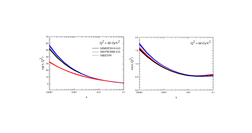
Figure 2: The integrated gluon and up quark distribution functions (see the text for detail).

As it was described in the section $II$, the $KMR$ approach was developed to calculate the $UPDF$, by using the given the global fitted $PDF$ as the input. To make the comparison more clear, the typical inputs, the gluon and the up quark $PDF$ considering the $PDF$ uncertainties at scale $Q^{2}$ = $60$ $GeV^{2}$, by using the $MRST99$ MRST , $MSTW2008$-$LO$ MSTW and $MMHT2014$-$LO$ 22 , are plotted in the figure 2.

The behavior of these integrated $PDF$ were discussed in detail in the related references MRST ; MSTW ; 22 . The $MMHT2014$ $PDF$ supersede the $MSTW2008$ parton sets and these $MSTW2008$ $PDF$ supersede the previously available $MRST$ sets. Also, as shown in the figure 2, these three sets are different at the very low $x$ region, that is the region where the transverse momentum becomes important. Especially for the gluons, the $MRST$ parton sets are very different from the other collaborations. Given the above mentioned issues, to study the effect of increasing the contribution of the gluon and the process of evolution in the $MRST$ set, we were motivated to consider all of these three sets of $PDF$ in our calculations. They are different (especially for the gluons $PDF$) at very low $x$ regions (this is the region where the transverse momentum becomes important) and they look similar at the large $x$ regions.

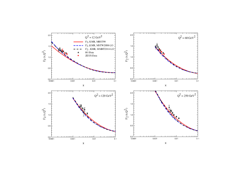
Figure 3: The proton structure functions $F_{2}(x,Q^{2})$ based on the integral form of the $KMR$ approach with the $AOC$ constraint as a function of $x$ for various $Q^{2}$ values, by using the $MRST99$ MRST , the $MSTW2008$- $LO$ MSTW and the $MMHT2014$-$LO$ 22 as the inputs, are compared with the $ZEUS$ ZEUS and $H1$ H1 experimental data.

Respectively, in the figures 3 and 4, the proton structure functions ($F_{2}(x,Q^{2})$) and the proton longitudinal structure functions ($F_{L}(x,Q^{2})$) in the framework of the integral form of the $KMR$ approach with the application of the $AOC$ constraint, by using central values of the $MRST99$, the $MSTW2008$- $LO$ and $MMHT2014$-$LO$ $PDF$ inputs, versus $x$, for $Q^{2}$ = $12$, $60$, $120$ and $250$ $GeV^{2}$ are plotted. Then, the predictions of this approach for the proton structure functions ($F_{2}(x,Q^{2})$) and the proton longitudinal structure functions ($F_{L}(x,Q^{2})$) are compared to the recent measurements of $ZEUS$ ZEUS and $H1$ H1 experimental data.

The results emphasize that (as it was shown in the references 14 ; 15 ; 16 ; 17 ; 18 ; 19 ), the $KMR$ approach suppresses the discrepancies between the inputs $PDF$, in which the presence of cutoff $AOC$ ($\Delta=\frac{k_{t}}{Q+k_{t}}$) has the key role. This property leads the outputs $UPDF$ which are more similar. As a result, the $UPDF$ generated via applying three different inputs $PDF$ have less discrepancies and in turn, each sets of $F_{2}(x,Q^{2})$ or $F_{L}(x,Q^{2})$ values with above $PDF$ are very close to each other. Although, in all of the panels of the figures 3 and 4, the discrepancies grow up with reduction of $x$ but it happens at very lower rate than the $PDF$ themselves (see the figures 2).

It should be noted that the results of using the $MMHT2014$-$LO$ $PDF$ and the $MSTW2008$- $LO$ $PDF$ inputs at very low $x$ regions are closer to the experimental data than the inputs of the $MRST99$. This indicates that inclusion of more gluons in the very small $x$ region is important (see panels $Q^{2}$ = 12 $GeV^{2}$ in the figures 3 and 4).

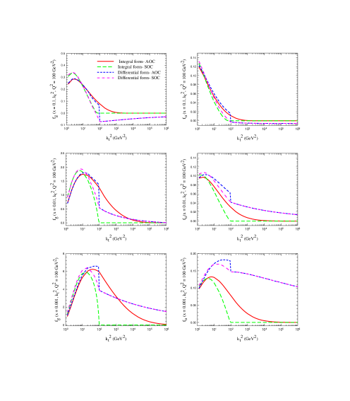
Figure 5: The gluon and up quark $UPDF$ as a function of $k_{t}^{2}$ ($GeV^{2}$) for the different versions of the $KMR$ approach with the $AOC$ and $SOC$ constraints and $x$ = 0.1, 0.01 and 0.001.

In the different panels of the figure 5, similar to 18 ; 19 ; GBS , (note that in reference GBS $xf_{g}(x,k_{t}^{2},Q^{2})/k_{t}^{2}$ is plotted), we plot the $UPDF$ (for the gluon and the up quark) with the input $MMHT2014$-$LO$ $PDF$ as a function of $k_{t}^{2}$ ($GeV^{2}$) for the two types of constraint discussed in the section $II$, i.e. $AOC$ and $SOC$, using the differential and integral forms of the $KMR$ approach. The hard scale is $Q^{2}=100$ $GeV^{2}$ and $x$ = 0.1, 0.01 and 0.001.

Despite seemingly mathematical equivalence between the differential and integral forms of $KMR$ prescription with the same constraints, the differences between them are manifested for the smaller $x$ values at the smaller transverse momentums (see that in gluon panels, the $UPDF$ of the two different versions with $AOC$ constraint separated from each other at $k_{t}^{2}\simeq{2,7}$ and 30 $GeV^{2}$ for the $x$ = 0.001, 0.01 and 0.1, respectively). As $GBS$ reported, this difference is due to the fact that we used the usual global fitted $PDF$ instead of the cutoff dependent $PDF$ for generating the $UPDF$. As we expect from the relation of $x$ and $\Delta$ discussed in the section $II$, the $SOC$ integral $UPDF$ become zero, when the transverse momentums become equal to the hard scale while those of $AOC$ smoothly go to zero for large transverse momentum.

But despite our expectation, the $SOC$ differential $UPDF$ with the global fitted $PDF$ as the input are nonzero for $k_{t}>Q$. Because in this region, as discussed in the Section $II$, $T_{a}(k_{t},Q)$ is considered to be unity, and the differential form of $KMR$ prescription (equation 6 ) turns into the equation (7) which is independent of the cutoff for the global fitted $PDF$ as the input. As a result, as shown in the various panels in the figure 5, the differential $UPDF$ with $SOC$ and $AOC$ for $k_{t}>Q$ are the same and at the very large transverse momentums becomes larger than the $AOC$ integral $UPDF$ (see panels $x$=0.01, 0.001). Also, as $GBS$ reported, the differential version of $KMR$ prescription with the different constraints with the the usual global fitted $PDF$ as the input leads to some un-physical results for large transverse momenta values. They are negative at $k_{t}>Q$ for panels $x$=0.1 and discontinuous at $k_{t}=Q$, that is a result of the discontinuity of the first derivative of the Sudakov form factor at $k_{t}=Q$.

But, the curves obtained from the integral form for both constraints behave in a smooth way without any un-physical results. Therefore, as we pointed out above, and that the integral form $KMR$-$UPDF$ by using the ordinary $PDF$ and the cutoff dependent $PDF$ as inputs, gives approximately the same results (as the $GBS$ report), if we intend to use the usual global fitted $PDF$ as the input for generating the $UPDF$, we can use only the integral version of $KMR$ prescription.

The proton structure function ($F_{2}(x,Q^{2})$) and the proton longitudinal structure functions ($F_{L}(x,Q^{2})$) by using the integral and differential versions of the $KMR$ $k_{t}$-factorization procedure for the $AOC$ and $SOC$ cutoffs are plotted in the figures 6 and 7 at hard scale 12, 60, 120 and 250 $GeV^{2}$, respectively. The $F_{2}(x,Q^{2})$ of the $LO$ collinear procedure and the experimental data of $H1$ and $ZEUS$ are also given for comparison.

As the energy scale increase the difference between the integral forms with the $AOC$ and $SOC$ cutoffs become more and those are separated from each other specially at small $x$ values and the $SOC$ results are below those of $AOC$. As far as present data are concerned, the $AOC$ results are much more closer to the data with respect to the $SOC$ cases. Regarding that the differential $UPDF$ with $SOC$ and $AOC$ for $k_{t}>Q$ are the same and at the very large transverse momentums becomes larger than the $AOC$ integral $UPDF$, the calculated proton structure functions and the proton longitudinal structure functions based on the $UPDF$ of the differential $KMR$ approach with $SOC$ and $AOC$ are the same by a good approximation and larger than those based on the $UPDF$ of the integral $KMR$ approach with $AOC$ at very small $x$ regions. Interestingly, despite some un-physical results for the differential form by using the usual global fitted $PDF$ as the input, approximately, the proton structure functions and the proton longitudinal structure functions based on the differential $UPDF$ are consistent with the experimental data. By comparing the curves of the figure 6, it turns out that integral form of $KMR$ prescription with $AOC$ is more consistent with the experimental data and the pure $LO$ collinear procedure than the others. Therefore, our structure function calculations in the framework of the integral form of the $KMR$ approach for the $AOC$ constraint confirm the conclusion which was made by $GBS$ that it is possible to use the usual global fitted $PDF$ instead of the cutoff dependent $PDF$ for generating the $UPDF$ of the $KMR$ approach by a good approximation.

In conclusion, it was shown that calculated proton structure functions and the proton longitudinal structure functions based on the $UPDF$ of the integral version of the $KMR$ approach for the $AOC$ constraint are reasonably consistent with the experimental data and, by a good approximation, they are independent to the input $PDF$. Therefore, they can be widely used in the calculations related to the particle physics phenomenology m1 . On the other hand, even the $k_{t}$-factorization and the $KMR$ approach can explain the shadowing effect in nuclei better than other nuclear physics indications m2 ; m3 . On the other hand, different constraints cutoffs were investigated using the the integral and the differential formulations of the $KMR$ prescription. The results confirm the statement made by the $GBS$ that: (1) According to the compatibility of the proton structure functions generated using $AOC$ integral $UPDF$ with the ordinary $PDF$ (the usual global fitted $PDF$) as the input, with the experimental data, it can be concluded that it is possible to use the usual global fitted $PDF$ instead of the cutoff dependent $PDF$ for generating the $UPDF$, especially because to fit the $PDF$ through the $UPDF$ is the cumbersome task. (2) As we pointed out above, due to some un-physical results for the differential form by using the ordinary $PDF$ as the input, as far as one used the integral form of the $KMR$ approach and the $AOC$ by using the ordinary $PDF$ as the input, there would not be any problem for the calculations of structure functions and hadron-hadron cross section in the framework of the $k_{t}$-factorization.

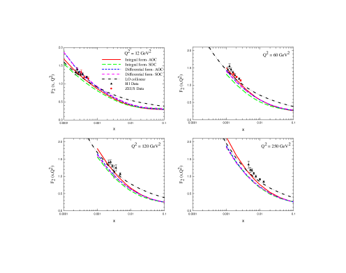
Figure 6: The proton structure functions $F_{2}(x,Q^{2})$ based on the different versions of the $KMR$ approach as a function of $x$ for various $Q^{2}$ values, by using the $MMHT2014$-$LO$ 22 $PDF$ as the inputs and the $AOC$ and $SOC$ constraints in comparison with the $F_{2}(x,Q^{2})$ of the $LO$ collinear procedure with the input $MMHT2014$-$LO$ $PDF$ and the $ZEUS$ ZEUS and $H1$ H1 experimental data.

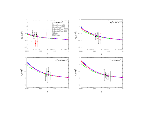
Figure 7: The proton longitudinal structure functions $F_{L}(x,Q^{2})$ based on the different versions of the $KMR$ approach as a function of $x$ for various $Q^{2}$ values, by using the $MMHT2014$-$LO$ 22 $PDF$ as the inputs and the $AOC$ and $SOC$ constraints in comparison with the $ZEUS$ ZEUS and $H1$ H1 experimental data.

References

• (1) V. N. Gribov and L. N. Lipatov, Yad. Fiz. (1972) 781.
• (2) L. N. Lipatov, Sov. J. Nucl. Phys. 20 (1975) 94.
• (3) G. Altarelli and G. Parisi, Nucl. Phys. B 126 (1977) 298.
• (4) Y. L. Dokshitzer, Sov. Phys. JETP 46 (1977) 641.
• (5) M. Ciafaloni, Nucl. Phys. B 296 (1988) 49 .
• (6) S. Catani, F. Fiorani, and G. Marchesini, Phys. Lett. B 234 (1990) 339.
• (7) S. Catani, F. Fiorani, and G. Marchesini, Nucl. Phys. B 336 (1990) 18.
• (8) G. Marchesini, Nucl. Phys. B 445 (1995) 49.
• (9) M. A. Kimber, A. D. Martin, M. G. Ryskin, Eur. Phys. J. C 12 (2000) 655.
• (10) G. Marchesini and B. R. Webber, Nucl. Phys. B 310 (1988) 461.
• (11) M. A. Kimber, A. D. Martin, and M. G. Ryskin, Phys. Rev. D 63 (2001) 114027.
• (12) M. Modarres, H. Hosseinkhani, N. Olanj, M.R. Masouminia, Eur. Phys. J. C 75 (2015) 556.
• (13) M. Modarres, H. Hosseinkhani, and N. Olanj, Phys. Rev. D 89 (2014) 034015.
• (14) M. Modarres, M. R. Masouminia, H. Hoseinkhani, N. Olanj, Nucl. Phys. A 945 (2016) 168.
• (15) A. D. Martin, R. G. Roberts, W. J. Stirling and R. S. Thorne, Eur. Phys. J. C 14 (2000) 133.
• (16) A. D. Martin, W. J. Stirling, R. S. Thorne and G. Watt, Eur. Phys. J. C 63 (2009) 189.
• (17) M. Modarres, M. R. Masouminia, R. Aminzadeh-Nik, H. Hoseinkhani, N. Olanj, Phys. Rev. D 94 (2016) 074035.
• (18) M. Modarres, M. R. Masouminia, R. Aminzadeh-Nik, H. Hoseinkhani, N. Olanj, Phys. Lett. B 772 (2017) 534.
• (19) M. Modarres, M. R. Masouminia, R. Aminzadeh-Nik, H. Hoseinkhani, N. Olanj, Nucl. Phys. B 926 (2018) 406.
• (20) M. Modarres, M. R. Masouminia, R. Aminzadeh-Nik, H. Hoseinkhani, N. Olanj, Nucl. Phys. B 922 (2017) 94.
• (21) K. Golec-Biernat, A. M. Stasto, Phys. Lett. B 781 (2018) 633.
• (22) M. A. Kimber, J. Kwiecinski, A. D. Martin, A. M. Stasto, Phys. Rev. D 62 (2000) 094006.
• (23) G. Watt, A. D. Martin, and M. G. Ryskin, Phys. Rev. D 70 (2004) 014012.
• (24) L. A. Harland-Lang, A. D. Martin, P. Motylinski, R. S. Thorne, Eur. Phys. J. C 75 (2015) 204.
• (25) ZEUS Collaboration, H. Abramowicz et al., Phys. Rev. D 90 (2014) 072002.
• (26) H1 Collaboration, V. Andreev et al., Eur. Phys. J. C 74 (2014) 2814.
• (27) V. S. Fadin, E. A. Kuraev, L. N. Lipatov, Phys. Lett. B 60 (1975) 50.
• (28) Ya. Ya. Balitsky, L. N. Lipatov, Sov. J. Nucl. Phys. 28 (1978) 822.
• (29) S. Catani, M. Ciafaloni and F. Hautmann, Phys. Lett. B 242 (1990) 97.
• (30) S. Catani and F. Hautmann, Nucl. Phys. B 427 (1994) 475.
• (31) M. Ciafaloni, Phys. Lett. 356 (1995) 74.
• (32) G. Watt, A. D. Martin, and M. G. Ryskin, Eur. Phys. J. C 31 (2003) 73.
• (33) J. Kwiecinski, A. D. Martin, and A. M. Stasto, Phys. Rev. D 56 (1997) 3991.
• (34) A. J. Askew, J. Kwiecinski, A. D. Martin and P. J. Sutton, Phys. Rev. D 47 (1993) 3775.
• (35) A.M. Stasto, Acta. Phys. Polo. B 27 (1996) 1353.
• (36) A. J. Askew, J. Kwiecinski, A. D. Martin and P. J. Sutton, Phys. Rev. D 49 (1994) 4402.
• (37) K. Golec-Biernat, A. M. Stasto, Phys. Rev. D 80 (2009) 014006.
• (38) M. Modarres, H. Hosseinkhani, and N. Olanj, Nucl. Phys. A 902 (2013) 21.
• (39) M. Modarres and H. Hosseinkhani, Few-Body Syst. 47 (2010) 237.
• (40) M. Modarres and H. Hosseinkhani, Nucl. Phys. A 815 (2009) 40.
• (41) H. Hosseinkhani and M. Modarres, Phys. Lett. B 694 (2011) 355.
• (42) H. Hosseinkhani and M. Modarres, Phys. Lett. B 708 (2012) 75.
• (43) R. Aminzadeh-Nik, M. Modarres, M. R. Masouminia, Phys. Rev. D 97 (2018) 096012.
• (44) M. Modarres and H. Hadian, Phys. Rev. D 98 (2018) 076001.
• (45) M. Modarres and H. Hadian, Nucl. Phys. A 983 (2019) 118.
Refer to caption