Dirac branes for Dirichlet branes: Supergravity actions

Abstract

Nontrivial Bianchi identities with local magnetic sources are solved by recognizing that gauge potentials are sections rather than globally defined functions, but properly accounting for the source degrees of freedom requires a modification of the field strength. Following work by Teitelboim and by Cariglia and Lechner, we extend Dirac’s string formalism for monopoles to D-branes in type IIA and IIB string theory. We give novel derivations of brane-induced Chern-Simons terms in the supergravity actions, including a prescription for integrating over potentials in the presence of magnetic sources. We give a noncovariant formulation of the IIB theory, keeping only the independent degrees of freedom of the self-dual 4-form potential. Finally, it is well known that D8-branes source the mass parameter of IIA supergravity; we show that the additional couplings of the massive IIA supergravity, including on other D-brane worldvolumes, are a consequence of the corresponding Dirac branes.

I Introduction

In modern mathematical treatments, we recognize the vector potential of a gauge theory not as a globally defined function but as the section of a gauge fiber bundle Wu and Yang (1976a, b). In somewhat more pedestrian terms, the vector potential can be defined as different vector-valued functions in different coordinate patches of spacetime as long as the distinct vector potentials are related by a gauge transformation on the overlap of the coordinate patches (we will refer to this as “gauge patching” of the vector potential). Gauge patching allows the description, for example, of a constant magnetic field strength on a torus (the distinct patches cover different unit cells) or the field of a magnetic monopole (where the Bianchi identity $dF_{2}\neq 0$ can have no globally defined solution). Analogs of both these examples for higher-rank form potentials are important in string theory as harmonic background flux in compactifications and higher-dimensional D-branes (and NS5-branes) that carry magnetic charges for the fundamental potentials. The coupling between the magnetic current and the potential is implicit in the patching and does not appear in the action for the magnetic charge.

An alternative that displays the coupling of magnetic sources explicitly is to double the number of gauge degrees of freedom by introducing dual field strengths and corresponding potentials. In this so-called “democratic” formalism, the magnetic sources enter in the equations of motion (EOM) for the dual potentials Bergshoeff et al. (2001). The extra degrees of freedom are then removed by enforcing duality conditions $F_{D-p-2}=\pm\star F_{p+2}$ at the level of the EOM. In the democratic formalism, the action for magnetic charges includes the same current-potential coupling as for electric charges, so the EOM of the magnetic charges includes the dual field strengths. Nontrivial Bianchi identities are enforced by the duality conditions. As a result, democratic formalisms still require gauge patching around magnetic sources.

Because the gauge transformations in the transition regions between gauge patches are part of the definition of the potentials and also depend on the dynamical magnetic currents, the gauge potentials are not independent degrees of freedom — they have a hidden dependence on the magnetic brane degrees of freedom which should be considered explicit in the language of calculus of variations. In quantum mechanical language, we need to separate the brane and gauge degrees of freedom to serve as integration variables in the path integral.

Interestingly, Dirac Dirac (1948) provided a solution in his early work on magnetic monopoles, which Teitelboim Teitelboim (1986), Bandos et al. Bandos et al. (1998), and Lechner and co-workers Lechner and Marchetti (2001a, b); Lechner et al. (2002); Cariglia and Lechner (2002); Lechner and Marchetti (2003); Lechner (2004); Cariglia and Lechner (2004) extended to magnetic $p$-branes. The key idea is as follows: Consider a field strength $\tilde{F}_{p+2}$ satisfying Bianchi identity $d\tilde{F}_{p+2}=\beta\star j_{D-p-3}$ with $\beta$ a sign convention. Any conserved current can be written as $\star j_{D-p-3}=d\star J_{D-p-2}$, so a field strength defined as $\tilde{F}_{p+2}\equiv dC_{p+1}+\beta\star J_{D-p-2}$ satisfies the Bianchi identity; in this way, the magnetic coupling appears in the action. There is actually one additional subtlety when the branes fill all noncompact dimensions; $\star j_{D-p-3}=d\star J_{D-p-2}$ on a compact manifold is inconsistent when there is net local charge, so we must define instead $\star j_{D-p-3}-\star j_{D-p-3}^{*}=d\star J_{D-p-2}$, where $j_{D-p-3}^{*}$ is some specified reference current (see Cownden and Frey (2018) for details in the case of magnetic monopoles). Now, $C_{p+1}$ is patched around the reference current, so dynamics of $j_{D-p-3}$ do not affect the potential. The alert reader may note that a Gauss law constraint means that the net charge must vanish on a compact manifold, but in string theory charge may dissolve in background flux, so the net charge of local objects need not vanish. Reference currents are necessary to account for this fact.

There are a variety of choices for the form $J$ for a given magnetically charged $p$-brane with worldvolume $\mathcal{M}$ and current $j_{\mathcal{M}}$. As described by Teitelboim (1986), we can consider a “Dirac $(p+1)$-brane” with worldvolume $\mathcal{N}$ of boundary $\partial\mathcal{N}=\mathcal{M}-\mathcal{M}^{*}$. Then $J_{\mathcal{N}}$, the current of the Dirac brane, satisfies $d\star J_{\mathcal{N}}=\star(j_{\mathcal{M}}-j_{\mathcal{M}^{*}})$. As we will see below, both the brane and Dirac brane currents are delta-function supported. A less singular option for $J$, used by Lechner et al. (2002); Cariglia and Lechner (2002); Lechner and Marchetti (2003); Lechner (2004); Cariglia and Lechner (2004), is given by the Chern kernel Chern (1944, 1945), which diverges only as a power law near the current $j_{\mathcal{M}}$. In the following, we will mostly remain agnostic about the nature of $J$, as our results are independent of this choice, but we will often use the language of Dirac branes to be concrete and refer to $J$ as the Dirac brane current as shorthand. It is also worth noting that, even fixing to Dirac branes or Chern kernels, $J$ is arbitrary up to its co-derivative, but the field strength $\tilde{F}$ is invariant.

Our goal is to extend this formalism to D-branes in the IIA and IIB string theories, writing these theories in terms of Ramond-Ramond (RR) potentials $C_{p+1}$ for $p\leq 3$. While Cariglia and Lechner (2004) have already considered (arbitrary intersections of) D-branes in the IIB theory by means of an anomaly argument, we present a new derivation via duality from the democratic formulation. In fact, Cariglia and Lechner (2004) found several new brane-induced terms in the IIB supergravity action, beyond the standard coupling between currents and potentials, ie, the Wess-Zumino (WZ) action for the D-branes. One set of new terms couples the Dirac brane currents of magnetic branes to those of electric branes; Deser et al. (1998) first identified the analogous term in Maxwell electrodynamics. These terms are related to charge quantization. Further, Cariglia and Lechner (2004) found a correction to the bulk Chern-Simons (CS) term involving Dirac brane currents. We will emphasize how these terms are required for consistency of the EOM and for gauge invariance. A key point in this story is that D-brane currents are not conserved due to the WZ couplings, but CS terms in the EOM and Bianchi identities cancel the anomaly via an inflow argument Witten (1996); Uranga (2002); we give a detailed accounting of the anomaly inflow in a general theory similar to that of the RR forms. The necessity of reference currents also forces us to explain what it means to integrate over a gauge-patched potential.

The plan of this paper is as follows. In section II, we demonstrate the anomaly inflow argument of Witten (1996); Uranga (2002) for a class of theories of form potentials which includes the RR potentials of both type II supergravities. We pay particular attention to how the inflow argument requires specific relations between various conventional coefficients in the EOM and Bianchi identity and confirm the consistency of the Dirac brane current with the inflow. Then we consider an action principle for the generalized theory of section II and introduce the modified CS term in section III through a novel derivation. In section IV, preliminary to our discussion of the supergravity actions, we find a prescription for integrating potentials that are gauge patched around magnetic sources, focusing on RR potentials in the 10D supergravities. We then give a novel derivation of the new terms in the type IIB supergravity action that were first described in Cariglia and Lechner (2004) in section V. We also eliminate redundant degrees of freedom in the self-dual 4-form potential, leading to a noncovariant action for the RR fields and discuss gauge invariance. Finally, in section VI, we derive the IIA supergravity action including the Romans mass term Romans (1986) and D-branes for the first time. It has long been known that D8-branes source the Romans mass, and we show for the first time how the corresponding Dirac 9-brane currents reproduce the additional couplings of the massive IIA supergravity. We also propose that additional WZ couplings on D-branes in the massive theory Bergshoeff and De Roo (1996); Green et al. (1996) are a consequence of the Dirac brane currents and conjecture the presence of other new WZ couplings on type IIA D-branes. We conclude with a brief discussion of future directions and give our conventions and some auxiliary results in the appendices. A forthcoming companion paper Frey (2020) will demonstrate how Dirac’s formalism separates the brane and gauge degrees of freedom in a form useful for dimensional reduction.

II Currents and anomaly inflow

In this section, we describe general brane currents and when they are not conserved. We then see how anomaly inflow determines the coefficients of several terms in the EOM and Bianchi identities and verify that the inflow mechanism is always consistent with the Dirac brane formalism. Finally, we apply our results to the 10D type II supergravity theories, making explicit the allowed, self-consistent sign conventions.

II.1 Currents and anomalies

Mathematically speaking, currents are dual vectors to differential forms (see Griffiths and Harris (1994) for a review), which includes form integration over submanifolds of the appropriate dimensionality. In this respect, the WZ action of a $p$-brane is the sum of $n$-currents acting on $n$-form potentials:

$$S_{WZ} = \sum_{q=0}^{p+1}\Gamma_{\mathcal{M}_{p+1},\mathcal{G}_{q}^{(p)}}(C_{p+1-q})$$

$$= \mu_{p}\int_{\mathcal{M}}\left(\sum_{q=0}^{p+1}[C_{p+1-q}]\wedge\mathcal{G}_{q}^{(p)}\right)=\mu_{p}\int_{\mathcal{M}}\,[C]\wedge\mathcal{G}^{(p)},$$

where $\mathcal{M}_{p+1}$ is the worldvolume, $\mathcal{G}_{q}$ are a series of worldvolume $q$-forms defined on the brane, and $\mu_{p}$ is the $p$-brane charge. These may be defined to include pullbacks of spacetime forms. After the second equality, we have defined $C$ and $\mathcal{G}^{(p)}$ as formal sums over the various rank forms [we will suppress the superscript $(p)$ on $\mathcal{G}$ when the dimensionality or type of brane is clear from context].

Of course, the WZ action (II.1) only describes a brane’s electric couplings to the gauge fields. This is sufficient in a democratic formulation but potentials of all ranks do not exist when only independent degrees of freedom are included. As a result, a spacetime description of currents is crucial. Since any dual vector $\Gamma_{n}$ is uniquely identified with a differential form $j_{n}$ by the inner product

$$\Gamma_{\mathcal{M},\mathcal{G}}(C_{n})\equiv\int C_{n}\wedge\star j_{\mathcal{M},\mathcal{G}}$$ (2)

with the integration over spacetime, we can identify the $j_{\mathcal{M},\mathcal{G}}$ as the brane currents. Then the EOM and Bianchi identity

$$d\star\tilde{F}_{p+2} = (-1)^{D-p-1}\star j_{p+1}+\cdots\quad\text{and}$$

$$d\tilde{F}_{p+2} = \beta_{p}\star j_{D-p-3}+\cdots$$ (3)

give the electric and magnetic couplings, where $\beta_{p}$ is a sign chosen by convention. The current $j_{p+1}=\sum j_{\mathcal{M}_{p+q+1},\mathcal{G}_{q}}$ with the sum over all branes. (On the flip side, all the currents of the same brane can be written as a formal sum $j_{\mathcal{M}}=\sum_{q}j_{\mathcal{M},\mathcal{G}_{q}}$.)

Naively, the current for a $(p+q)$-brane with worldvolume form $\mathcal{G}_{q}$ is

$$j^{\mu_{1}\cdots\mu_{p+1}}_{\mathcal{M},\mathcal{G}}(x)=\mu_{p+q}\int_{\mathcal{M}_{p+q=1}}\hat{d}X^{\mu_{1}}\wedge\cdots\hat{d}X^{\mu_{p+1}}\wedge\mathcal{G}_{q}\,\delta^{D}(x,X),$$ (5)

where $X^{\mu}$ are the embedding coordinates. This may be modified in topologically nontrivial situations, such as when the brane in question is actually the nontransversal intersection of two other branes. Nontransversal intersections are the focus of Cheung and Yin (1998); Lechner (2004); Cariglia and Lechner (2004). As our goal is to emphasize writing the action in terms of independent degrees of freedom, we base our results on the naive current (5); the adaptation to nontransversal intersections follows from Cariglia and Lechner (2004).

The anomalies we consider are local in nature, so they must cancel pointwise. While related, we emphasize that these anomalies are separate from global anomalies that forbid certain brane configurations, such as the Freed-Witten anomaly Freed and Witten (1999) or the magnetic D-brane Gauss law constraint that $H_{3}$ integrate to zero over the worldvolume (see Frey and Polchinski (2002); Kashani-Poor and Tomasiello (2005)). From the perspective of the WZ action (II.1), they arise from a gauge variation $\delta C=d\lambda$. Integrating the pullback by parts yields a term from the brane boundary and one from $\hat{d}\mathcal{G}$. In some cases, these can cancel between branes; for example, a D1-brane can end on a D3-brane, providing a magnetic source for the D3-brane gauge field. The two anomalous terms cancel in the summed current $j_{2}$. However, if $\hat{d}\mathcal{G}$ contains the pullback of a spacetime form, the cancellation must be by inflow associated with a modified gauge transformation $\delta C$ as occurs in string theory.

From a spacetime point of view, we can consider the divergence of the brane current

$$(\star d\star j_{\mathcal{M},\mathcal{G}})^{\mu_{1}\cdots\mu_{p}} = (-1)^{(p+1)(D-p)}\mu_{p+q}\int_{\mathcal{M}}\nabla_{\nu}\left[\delta^{D}(x,X)\hat{d}X^{\nu}\wedge\hat{d}X^{\mu_{1}}\wedge\cdots\hat{d}X^{\mu_{p}}\wedge\mathcal{G}_{q}\right]$$ (6)

$$= (-1)^{D(p+1)+1}\mu_{p+q}\int_{\mathcal{M}}\hat{d}\left[\delta^{D}(x,X)\hat{d}X^{\mu_{1}}\wedge\cdots\hat{d}X^{\mu_{p}}\wedge\mathcal{G}_{q}\right]$$

$$+(-1)^{D(p+1)+p}\mu_{p+q}\int_{\mathcal{M}}\hat{d}X^{\mu_{1}}\wedge\cdots\hat{d}X^{\mu_{p}}\wedge\hat{d}\mathcal{G}_{q}\,\delta^{D}(x,X)\ .$$

In an arbitrary Lorentzian metric, $\delta^{D}(x,X)$ is the biscalar distribution, and the covariant derivative acts with respect to the spacetime position $x$, but the derivative switches to the partial with respect to $X$ as described in Poisson et al. (2011). We therefore see that the brane currents are not conserved:

$$d\star j_{\mathcal{M},\mathcal{G}}=(-1)^{D+q}\star\tilde{\jmath}_{\partial\mathcal{M},\mathcal{G}}-(-1)^{D}\star j_{\mathcal{M},\hat{d}\mathcal{G}},$$ (7)

where $\tilde{\jmath}$ is a $p$-form current for the boundary of the worldvolume. Henceforth in this paper, we will assume that the boundary contributions cancel with some of the worldvolume $\hat{d}\mathcal{G}$ contributions, so we will ignore those terms from here out, returning to them in the companion paper Frey (2020).

Consider then a single brane (ie, $\partial\mathcal{M}=0$) with $\hat{d}\mathcal{G}$ a pullback of a nontrivial spacetime form $H_{r+1}$. We will find that the anomalies cancel when $\hat{d}\mathcal{G}_{q}=\sum_{r}\eta_{p,q,r}[H_{r+1}]\mathcal{G}_{q-r}$, where $H_{r+1}$ is prototypically the field strength of a potential that does not couple to the branes, and $\eta_{p,q,r}$ is some proportionality constant. Then, using (66),

$$\star j_{\mathcal{M},[H_{r+1}]\mathcal{G}_{q-r}} = \star\left(j_{\mathcal{M},\mathcal{G}_{q-r}}\cdot H_{r+1}\right)$$

$$= (-1)^{(r+1)(D-r-1)}H_{r+1}\wedge\star j_{\mathcal{M},\mathcal{G}_{q-r}}.$$

We will find that $\eta$ is independent of the rank $q$ of the worldvolume forms, so the anomaly for the total brane current is conveniently written as

$$d\star j_{p+1}=\sum_{r}(-1)^{r(D-r)}\eta_{p,r}H_{r+1}\wedge\star j_{p+r+1}.$$ (9)

II.2 Anomaly inflow

We consider a set of potentials $C_{p+1}$ (the RR potentials in string theory) and corresponding gauge-invariant field strengths $\tilde{F}_{p+2}$, with an additional set of field strengths $H_{r+1}=dB_{r}$ assumed closed with pullbacks $[H_{r+1}]$ that appear in $\hat{d}\mathcal{G}$ for some branes (with this coupling, those branes carry an electric current for $B_{r}$, but $H_{r+1}$ remains closed). The classical anomaly discussed in the previous section then appears in the current whenever $H_{r+1}\neq 0$, whether it is a topologically nontrivial flux or due to another brane source. It is a simple generalization to add an extra index to $C$ or $B$ to have more than one potential at each rank. Our discussion of the inflow is similar to comments by Witten (1996) for M-theory and is implicit in Cariglia and Lechner (2004) for IIB string theory; Uranga (2002) gives a worldvolume argument for string theory. We are not aware of a discussion in this full class of theories.

The general EOM for $C_{p+1}$ (to first order in $\tilde{F}_{p+2}$) has the structure

$$d\star\tilde{F}_{p+2} = (-1)^{D-p-1}\star j_{p+1}$$ (10)

$$+\sum_{r=0}^{D-p-3}\left[\alpha_{p,r}(\star\tilde{F}_{p+r+2})\wedge H_{r+1}\right.$$

$$\left.+\tilde{\alpha}_{p,r}\tilde{F}_{D-p-r-2}\wedge H_{r+1}\right],$$

where $\alpha,\tilde{\alpha}$ are constants. Meanwhile, the Bianchi identity is

$$d\tilde{F}_{p+2}=\beta_{p}\star j_{D-p-3}+\sum_{r=0}^{p+1}\tilde{\beta}_{p,r}\tilde{F}_{p-r+2}\wedge H_{r+1};$$ (11)

$\beta_{p}$ is a sign convention, which can be chosen independently for each field strength. For now, we treat the $\alpha,\tilde{\alpha},\beta,\tilde{\beta}$ as independent constants, though there are relations among them in a Lagrangian formulation of the theory; other conditions following from gauge invariance are discussed in appendix B. The $\tilde{\alpha}$ terms follow from CS terms in the action, while the $\alpha$ and $\tilde{\beta}$ terms arise from terms in the field strength. To distinguish them from CS terms, we will refer to the $\alpha$ and $\tilde{\beta}$ terms as “transgression” terms. Theories with this structure include of course the type II supergravities and also the dimensionally reduced theory of gravity and form potentials on a torus, for example.

Current (non)conservation is related to the integrability conditions obtained by taking the exterior derivative of the EOM and Bianchi identity. For the EOM, we have

$$d\star j_{p+1} = \sum_{r}\left[-(-1)^{r}\alpha_{p,r}+(-1)^{D-p}\tilde{\alpha}_{p,r}\beta_{D-p-r-4}\right]$$ (12)

$$\times\star j_{p+r+1}\wedge H_{r+1},$$

leaving off terms that are independent of the brane currents. In other words, we see that the derivatives of the CS and transgression terms localize on the currents as needed for an anomaly inflow. Comparing to equation (9), we find

$$\eta_{p,r}=-(-1)^{D+(p+1)(r+1)}\alpha_{p,r}-(-1)^{pr}\tilde{\alpha}_{p,r}\beta_{D-p-r-4}$$ (13)

since the anomaly must cancel when only one $H_{r+1}$ background is nonvanishing. In fact, this holds for any case where only one brane contributes to the current, so we see that $\eta$ is independent of the worldvolume form rank.

Similarly, the Bianchi identity yields

$$d\star j_{D-p-3}=-\beta_{p}\sum_{r}\tilde{\beta}_{p,r}\beta_{p-r}\star j_{D-p+r-3}\wedge H_{r+1}.$$ (14)

Cancellation of the anomaly then requires

$$\eta_{D-p-4,r}=(-1)^{r(D-p)+p}\beta_{p}\beta_{p-r}\tilde{\beta}_{p,r}.$$ (15)

Again, we see that $\eta$ is independent of $q$.

II.3 Dirac brane currents

We will now see how Dirac brane currents in the field strengths fit into the Bianchi identities using the constraint (15). Our discussion extends similar results in Cariglia and Lechner (2004).

To start, we need to consider how to extend the worldvolume form $\mathcal{G}$ from the brane worldvolume to the Dirac brane or, in the case $J$ represents a Chern kernel, the entire spacetime. The key point is to choose the reference brane worldvolume $\mathcal{M}^{*}$ homotopic to $\mathcal{M}$ (so $\mathcal{N}$ is continuous for a Dirac brane). The extension of $\mathcal{G}$ depends on its form. For D-branes, we will be concerned primarily with the case that $\mathcal{G}=\mathcal{G}([B_{2}],\hat{d}A_{1})$, where $A_{1}$ is the worldvolume gauge field. In this case, we continue to take $B_{2}$ as given by the spacetime NSNS form (pulled back to $\mathcal{N}$ as appropriate). For the gauge field, we choose a fixed $A_{1}^{*}$ on $\mathcal{M}^{*}$ and an extension $\bar{A}_{1}$ to $\mathcal{N}$ or spacetime that pulls back to $A_{1}$ on $\mathcal{M}$ and $A_{1}^{*}$ on $\mathcal{M}^{*}$. Then the Dirac brane current takes the form of (5) with $\mathcal{G}$ promoted to the extension $\bar{}\mathcal{G}$ and $X^{\mu}$ replaced by the embedding coordinates $Y^{\mu}$ of $\mathcal{N}$. For a Chern kernel of a $(p+q)$-brane, $\star J_{\bar{}\mathcal{G}}\equiv(-1)^{(p+1)(q+1)}(\star J)\bar{}\mathcal{G}$ (a similar formula holds for Dirac brane currents when $\bar{}\mathcal{G}$ is the pullback of a spacetime form by virtue of (66)).

Since the Dirac brane contribution to the field strength is given by the Dirac brane’s current, equation (7) applies in the form

$$d\star J_{\mathcal{N},\bar{}\mathcal{G}}=(-1)^{D+q}\star\left(j_{\mathcal{M},\mathcal{G}}-j_{\mathcal{M}^{*},\mathcal{G}}\right)-(-1)^{D}\star J_{\mathcal{N},\bar{d}\bar{}\mathcal{G}}.$$ (16)

Therefore, to cancel the dynamical current $j_{D-p-3}=\sum j_{\mathcal{M}_{D-p+q-1},\mathcal{G}_{q}}$ (summed over all branes) in the Bianchi identity (11), we should define

$$\tilde{F}_{p+2}=dC_{p+1}+(-1)^{D}\beta_{p}\star J_{D-p-2}+\sum_{r=0}^{p+1}\tilde{\beta}_{p,r}C_{p-r+1}\wedge H_{r+1},$$ (17)

where the Dirac brane current is a sum over the corresponding Dirac branes

$$J_{D-p-2}=\sum(-1)^{q}J_{\mathcal{N}_{D-p+q-2},\bar{}\mathcal{G}_{q}}$$ (18)

and $C_{p+1}$ includes the potential for the reference current for worldvolumes $\mathcal{M}^{*}$. Then the current for the Dirac brane associated with a given physical brane can be written as a formal sum $J_{\mathcal{N}}=\sum_{q}(-1)^{q}J_{\mathcal{N},\bar{}\mathcal{G}_{q}}$.

With this definition for the total Dirac brane current, the divergence (16) and condition (15) give

$$d\star J_{D-p-2} = (-1)^{D}\star(j_{D-p-3}-j^{*}_{D-p-3})-\beta_{p}\sum_{q,r}(-1)^{q+(r+1)(p-r-1)}\tilde{\beta}_{p,r}\beta_{p-r}H_{r+1}\wedge\star J_{\mathcal{N},\bar{}\mathcal{G}_{q-r}}$$ (19)

$$= (-1)^{D}\star(j_{D-p-3}-j^{*}_{D-p-3})+\beta_{p}\sum_{r}\tilde{\beta}_{p,r}\beta_{p-r}\star J_{D-p+r-2}\wedge H_{r+1}.$$

Since $C_{p+1}$ contains the potential for the reference current,

$$d\tilde{F}_{p+2} = \beta_{p}\star j_{D-p-3}+\sum_{r}\tilde{\beta}_{p,r}\left(dC_{p-r+1}+\sum_{\ell}\tilde{\beta}_{p-r,\ell}C_{p-r-\ell+1}\wedge H_{\ell+1}+\beta_{p-r}\star J_{D-p+r-2}\right)\wedge H_{r+1}$$ (20)

$$= \beta_{p}\star j_{D-p-3}+\sum_{r}\tilde{\beta}_{p,r}\tilde{F}_{p-r+2}\wedge H_{r+1}.$$

In other words, the co-derivative of the Dirac brane current is precisely consistent with the appearance of Dirac brane currents in the transgression term.

II.4 Type II supergravity conventions

We can now apply our results to set limits on possible sign conventions in the 10D type II supergravities. Some of the restrictions we find below (such as the alternating of signs in the duality conditions for the democratic formulation) appear implicitly in the literature (see for example the discussion of conventions in appendix A of Andriot and Blåbäck (2017)), but we are not aware of an explicit derivation from first principles.

While the D-brane WZ action identifies

$$\mathcal{G}=e^{\mathcal{F}}\wedge\sqrt{\frac{\hat{A}(4\pi^{2}\alpha^{\prime}R_{T})}{\hat{A}(4\pi^{2}\alpha^{\prime}R_{N})}},$$ (21)

where $\mathcal{F}=2\pi\alpha^{\prime}F_{2}+\eta[B_{2}]$, $\hat{A}$ is the A-roof genus, and $R_{T},R_{N}$ are the tangent and normal bundle curvatures, we will not consider the $\alpha^{\prime}$ corrections, instead restricting to $\mathcal{G}=\exp\mathcal{F}$. See Cariglia and Lechner (2004) for more on $\alpha^{\prime}$ corrections in the IIB theory. Both type II supergravities in this approximation have a single background field strength $H_{3}=dB_{2}$ and, following from the above, a common sign choice $\eta=\eta_{p,2}$ appearing in $\mathcal{F}$ for all $p$. Here, we will also follow the typical choice of setting all $\tilde{\beta}_{p,2}\equiv\tilde{\beta}$, a single sign choice for the transgression terms in each theory.

Starting with the IIB theory with only potentials $C_{p+1}$ for $p\leq 3$, the EOM and Bianchi identities are

$$d\star\tilde{F}_{1} = \star j_{0}+\alpha_{-1}\star\tilde{F}_{3}\wedge H_{3},$$

$$d\tilde{F}_{1} = \beta_{-1}\star j_{8},$$

$$d\star\tilde{F}_{3} = \star j_{2}+(\alpha_{1}\star\tilde{F}_{5}+\tilde{\alpha}_{1}\tilde{F}_{5})\wedge H_{3},$$

$$d\tilde{F}_{3} = \beta_{1}\star j_{6}+\tilde{\beta}\tilde{F}_{1}\wedge H_{3},$$

$$d\star\tilde{F}_{5} = \star j_{4}+\tilde{\alpha}_{3}\tilde{F}_{3}\wedge H_{3},$$

$$d\tilde{F}_{5} = \beta_{3}\star j_{4}+\tilde{\beta}\tilde{F}_{3}\wedge H_{3}.$$ (22)

The appearance of both transgression and CS terms for the $\tilde{F}_{3}$ EOM is due to the self-duality condition on $\tilde{F}_{5}$. The constraint (13) tells us immediately that $\eta=-\alpha_{-1}=-\tilde{\alpha}_{3}\beta_{1}=-\alpha_{1}-\tilde{\alpha}_{1}\beta_{3}$. Meanwhile, the Bianchi identities are consistent with (15) for $\eta=-\beta_{-1}\beta_{1}\tilde{\beta}=-\beta_{1}\beta_{3}\tilde{\beta}$. Finally, the transgression terms in the EOM and Bianchi identity are related through variation of the Lagrangian, leading to equation (81), which implies $\alpha_{-1}=-\tilde{\beta}$ and $\eta=\tilde{\beta}$. All told, there are two independent sign choices, $\tilde{\beta}$ and $\beta_{3}$, with the signs in the Bianchi identities alternating $\beta_{3}=-\beta_{1}=\beta_{-1}$.

The type IIA supergravity (including a possible mass term) has

$$d\star\tilde{F}_{0} = 0,\quad d\tilde{F}_{0}=\beta_{-2}\star j_{9}$$

$$d\star\tilde{F}_{2} = -\star j_{1}+\alpha_{0}\star\tilde{F}_{4}\wedge H_{3},\quad d\tilde{F}_{2}=\beta_{0}\star j_{7}+\tilde{\beta}\tilde{F}_{0}\wedge H_{3}$$

$$d\star\tilde{F}_{4} = \star j_{4}+\tilde{\alpha}_{2}\tilde{F}_{4}\wedge H_{3},\quad d\tilde{F}_{4}=\beta_{2}\star j_{5}+\beta\tilde{F}_{2}\wedge H_{3}.$$ (23)

As in the IIB case, we find $\eta=\alpha_{0}=-\tilde{\alpha}_{2}\beta_{2}$ and $\eta\tilde{\beta}=\beta_{-2}\beta_{0}=\beta_{0}\beta_{2}$. Derivation of the transgression terms from the action gives also $\alpha_{0}=-\tilde{\beta}$, which tells us that $\eta=-\tilde{\beta}$ and $\beta_{0}=-\beta_{-2}=-\beta_{2}$. There are once again two independent sign choices, with the others determined.

In either supergravity, the democratic formulation has

$$d\star\tilde{F}_{p+2} = (-1)^{p+1}\star j_{p+1}+\alpha_{p}\star\tilde{F}_{p+4}\wedge H_{3},$$

$$d\tilde{F}_{p+2} = \beta_{p}\star j_{7-p}+\tilde{\beta}\tilde{F}_{p}\wedge H_{3}$$ (24)

for $-2\leq p\leq 8$ ($\tilde{F}_{p<0}\equiv 0$). By comparison to the Bianchi identities above, the duality relations must be $\star\tilde{F}_{D-p-2}=\mp\beta_{p}\tilde{F}_{p+2}$ (in IIA and IIB respectively) for $p\leq 3$; in particular, $C_{4}$ satisfies the self-duality relation $\star\tilde{F}_{5}=\beta_{3}\tilde{F}_{5}$. Since the coefficients $\beta_{p}$ alternate signs in each theory, so do the duality relations. Since the D-brane charge (vs antibrane) is determined by the WZ coupling to $C_{p+1}$ in the democratic formulation, these alternating signs mean that D$p$-branes with $p\geq 3$ enter the Bianchi identities with alternating signs as well. The signs can only be chosen the same if the transgression coefficients $\tilde{\beta}_{p}$ are distinct for the different $\tilde{F}_{p+2}$. Finally, since the Bianchi identities for the higher-rank field strengths have the same form, we have $\beta_{p}\beta_{p+2}=-1$ (i.e., alternating signs) for all $p$.

III Brane-modified Chern-Simons action

Chern-Simons terms are familiar from the actions of both 10D type II supergravities and the 11D supergravity. We emphasize here that the presence of D-branes necessarily modifies those CS terms; by extension (through duality, etc), M-branes in 11D and NS5-branes in 10D must also modify them. The CS term modifications were first pointed out by Cariglia and Lechner (2004); here we give a new, simple, physically-motivated derivation in the theory of the previous section, which we can apply to the 10D supergravities later.

The action

$$S = \frac{1}{2\kappa_{0}^{2}}\int\sum_{p}(-1)^{p(D-p)+1}\left[\frac{1}{2}\tilde{F}_{p+2}\wedge\star\tilde{F}_{p+2}\right.$$ (25)

$$\left.+(-1)^{D}C_{p+1}\wedge\star j_{p+1}\vphantom{\frac{1}{2}}\right]+S_{CS},$$

with Chern-Simons terms

$$S_{CS} = \frac{1}{2\kappa_{0}^{2}}\sum_{p,r}\int\left[\gamma_{p,r}C_{p+1}\wedge\tilde{F}_{D-p-r-2}\right.$$ (26)

$$\left.+\tilde{\gamma}_{p,r}(\star J_{D-p-2})\wedge C_{D-p-r-3}\vphantom{\tilde{F}}\right]\wedge H_{r+1}$$

reproduces the $C_{p+1}$ EOM (10), assuming that the field strength is defined by equation (17) with the Dirac brane current (18). $\gamma_{p,r},\tilde{\gamma}_{p,r}$ are some set of constants related to the EOM coefficients $\tilde{\alpha}_{p,r}$. We have ignored kinetic terms for the closed field strengths $H_{r+1}$ as well as the gravitational sector. The canonical coupling between the potential and electric current in (25) determines the sign of the source term in (10), and it also gives the WZ action for all the branes (i.e., there is no need for an additional WZ action on the branes) up to a factor of the gravitational coupling $2\kappa_{0}^{2}$, which can be accommodated by rescaling the brane charges.

We discuss the invariance of this action and the field strength (17) under the gauge transformations of $C_{p+1}$ in the absence of brane sources in appendix B, arriving at constraints (73,80), which also guarantee that the Bianchi identity and EOM depend only on $\tilde{F}_{p+2}$ rather than $C_{p+1}$ (in the absence of currents). We also find the relationships (81) between the EOM coefficients $\alpha_{p,r},\tilde{\alpha}_{p,r}$ and $\tilde{\beta}_{p,r},\gamma_{p,r}$ in the appendix.

While the $\gamma_{p,r}$ terms in $S_{CS}$ are familiar from, for example, the 10D supergravities, the $\tilde{\gamma}_{p,r}$ terms require some explanation. Without them, the Dirac brane currents are absent from the field strengths in the $\tilde{\alpha}_{p,r}$ terms of the EOM. That would leave the EOM dependent on the Dirac brane worldvolumes $\mathcal{N}$ including the arbitrary reference branes $\mathcal{M}^{*}$, which would clearly be inconsistent (in fact, that would be a violation of gauge invariance in the magnetic context). So we consider

$$\frac{\delta S_{CS}}{\delta C_{p+1}} = \sum_{r}\gamma_{p,r}\tilde{F}_{D-p-r-2}\wedge H_{r+1}$$

$$+\sum_{r}(-1)^{p(D-p-r)}\gamma_{D-p-r-4,r}\left(\tilde{F}_{D-p-r-2}\right.$$

$$\left.-(-1)^{D}\beta_{D-p-r-4}\star J_{p+r+2}\right.$$

$$\left.\vphantom{\tilde{F}}+(-1)^{(p+1)(D-p-r)}\tilde{\gamma}_{D-p-r-4,r}(\star J_{p+r+4})\right)\wedge H_{r+1}$$

assuming the coefficients obey (80). Therefore, we require $\tilde{\gamma}_{p,r}=(-1)^{D-p}\beta_{p}\gamma_{p,r}$ to ensure that the EOM are written only in terms of the field strengths.

We will later derive these and other new brane-induced terms for the type II supergravities.

IV Integrating patched potentials

It is not immediately clear what it means to integrate over a quantity including a potential with gauge patching because the potential is not single valued in the overlap of coordinate patches: Either gauge is physically acceptable. As a result, many authors, including Green et al. (1997); Cheung and Yin (1998); Cariglia and Lechner (2004) have suggested writing potential-current couplings in terms of the gauge-invariant field strength. However, if we attempt to write an action following that approach without the explicit appearance of the potentials, the EOM will contain the arbitrary reference currents $j^{*}_{p+1}$ (for electric sources). Consider, for example, the action (25) above with the replacement $C_{p+1}(\star j_{p+1})\to(-1)^{p}\tilde{F}_{p+1}(\star J_{p+2})$. Even ignoring transgression terms by setting $H_{r+1}\to 0$, the variation of this term is $\delta C_{p+1}\wedge\star(j_{p+1}-j_{p+1}^{*})$. Here we give what is to our knowledge the first description of how to carry out spacetime integrals including gauge-patched potentials.

The key idea is already present in Wu and Yang (1976b), who gave a prescription for integrating the vector potential of Maxwell theory along a charged particle worldline in the presence of a monopole. In sketch form our new prescription for integration against other forms over spacetime is as follows: Pick an arbitrary division where the integrated potential switches from one gauge to another. Then design the integral to be invariant under changes of the division, a choice closely related to gauge invariance. Since we are integrating over spacetime, we also have to exclude the locus of magnetic charge, where the potential is undefined.

For simplicity, we work with RR potentials in string theory. Specifically, we consider a set of potentials $C_{p+1}$ for $p$ either even or odd (as in the IIA or IIB supergravity respectively). Written as a formal sum of forms, the gauge-invariant field strengths are $F=dC+\tilde{\beta}CH_{3}$ and the gauge transformations are $\delta C=d\chi-\tilde{\beta}\chi H_{3}$, where $\tilde{\beta}$ is a single sign choice. Depending on the application, the formal sum $C$ could include $p=-1$ to $8$ as in a democratic formulation of the supergravity or only a subset (e.g., $p=0,2$ in type IIA supergravity). Taking $p=0,H_{3}=0$, our prescription also applies to standard electrodynamics. The field strengths do not include Dirac branes, and the Bianchi identities are $dF=\star(\beta j^{*})+\tilde{\beta}FH_{3}$, where $(\beta j^{*})=\sum_{p}\beta_{p}j_{p+1}^{*}$ with $\beta_{p}$ a distinct sign choice for each potential. Our results apply to any gauge-patched potential, meaning $j^{*}$ could represent dynamical currents, but we will take $j^{*}$ to be fixed reference currents. It is worth recalling that a high-dimension brane with a worldvolume gauge field or in the presence of nonvanishing $B_{2}$ contributes to lower-rank currents, so $j^{*}_{p+1}$ may include currents smeared over worldvolumes with dimension greater than $p+1$.

To define the spacetime integral $\int CK$, where $K$ is another formal sum of forms, we note that the potentials $C$ are undefined on the collection of branes that contribute to $j^{*}$. Contrast this to electric charges where potentials simply diverge; for the example of a magnetic monopole, none of the coordinate patches with well-defined potentials covers the monopole location. Therefore, rather than integrating over all of spacetime, we excise a small tube around the worldvolume of each magnetically charged brane with boundary $\mathcal{P}$. After integrating, we will take the volume of the excluded tube to vanish, so it becomes measure zero. In the presence of multiple magnetic brane sources, $\mathcal{P}$ has multiple components.

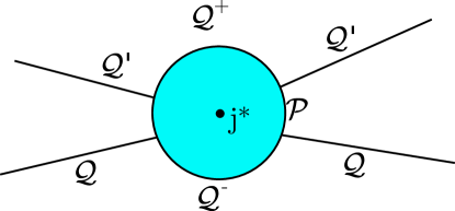
Figure 1: Sketch of integration region with magnetic current $j^{*}$. Shaded region inside $\mathcal{P}$ is excluded; $\mathcal{Q}$,$\mathcal{Q}^{\prime}$ are possible separations of two gauge patches.

Now consider the overlap region of two gauge patches (multiple gauge patches are a straightforward extension, assuming the configuration is simple enough) of potentials $C^{\pm}$ around some magnetic source. On the overlap region, the two potentials are related by the gauge transformation $C^{+}=C^{-}+d\zeta-\tilde{\beta}\zeta H_{3}$. We choose a codimension-one surface $\mathcal{Q}$ in the overlap region such that the spacetime volume $\mathcal{Q}^{\pm}$ on either side of $\mathcal{Q}$ is within the coordinate patch where $C^{\pm}$ is valid respectively. This is just a partition of spacetime into regions where each potential is used. Note that $\mathcal{Q}$ will generically intersect the boundary surface $\mathcal{P}$. In the example of a monopole, this is just related to the fact that the region where each potential is valid is given by a range of polar angle. Figure 1 sketches the various surfaces for a current $j^{*}$. Quantities integrated over $\mathcal{Q}$ or $\mathcal{P}$ are assumed to be pulled back to the appropriate submanifold.

We now define the spacetime integral as

$$\int C\wedge K\equiv\int_{\mathcal{Q}^{+}}C^{+}\wedge K+\int_{\mathcal{Q}^{-}}C^{-}\wedge K\pm\int_{\mathcal{Q}}\zeta\wedge K,$$ (28)

where the sign on the $\mathcal{Q}$ integral depends on the orientation of the integration measure. We will choose the positive sign below and take care to account for signs due to the orientation.

This is sensible provided that the integral is unchanged under changes of the arbitrary dividing surface $\mathcal{Q}$. Consider then changing $\mathcal{Q}\to\mathcal{Q}^{\prime}$. The change in the integral is

$$\int_{\mathcal{Q}}^{\mathcal{Q}^{\prime}}(C^{-}-C^{+})\wedge K+\int_{\mathcal{Q}^{\prime}}\zeta\wedge K-\int_{\mathcal{Q}}\zeta\wedge K$$

$$=\int_{\mathcal{Q}}^{\mathcal{Q}^{\prime}}\zeta\wedge\left[(-1)^{p}dK+\tilde{\beta}H_{3}\wedge K\right]-\int_{\bar{}\mathcal{P}}\zeta\wedge K,$$ (29)

where $\int_{\mathcal{Q}}^{\mathcal{Q}^{\prime}}$ indicates the region with boundary $\mathcal{Q}^{\prime}-\mathcal{Q}-\bar{}\mathcal{P}$ (that is, the region between $\mathcal{Q}$ and $\mathcal{Q}^{\prime}$ in figure 1) and $\bar{}\mathcal{P}$ is the region on $\mathcal{P}$ between its intersections with $\mathcal{Q},\mathcal{Q}^{\prime}$. This will vanish provided $dK+(-1)^{p}\tilde{\beta}H_{3}K=0$ and either $K$ has no delta-function-like singularity (so the $\bar{}\mathcal{P}$ integral vanishes as $\mathcal{P}$ shrinks) or $\zeta K=0$ (for example, due to the legs of each form). It is not a coincidence that $dK+(-1)^{p}\tilde{\beta}H_{3}K=0$ is the same condition for the integral (28) to be gauge invariant under gauge transformations $\chi$ that are globally defined over the integration region and vanish on the boundary at infinity and $\mathcal{P}$.

Maxwell electrodynamics provides some simple examples. Consider a static monopole of charge $g$ at the origin. Then the simplest form for $\mathcal{P}$ is a sphere of radius $\epsilon$ around the origin. With the typical choices $A_{1}^{\pm}=g(\pm 1-\cos\theta)d\phi$, $\mathcal{Q}$ is any surface that intersects $\mathcal{P}$ in the limit $\epsilon\to 0$ and does not intersect the $z$-axis. A simple choice for $Q$ is the $xy$-plane with transition function $\zeta=2g\phi$. This prescription for integration also works for harmonic flux with no magnetic sources on a compact manifold. For example, we can consider a constant magnetic field on a square $T^{2}$, which we can describe by vector potential $A_{1}=Bydx$ in the first unit cell $0\leq x,y<2\pi R$. To make the potential periodic in $y$, we must work in a different gauge in each unit cell given by $2\pi Rn\leq y<2\pi R(n+1)$ with gauge transition function $\zeta=-2\pi RBx$, but of course each gauge is valid over the entire covering space. To integrate over the first unit cell, we choose any curve $\mathcal{Q}$ that runs from $x=0$ to $x=2\pi R$ within the unit cell. A simple choice for $\mathcal{Q}$ is the $x$-axis.

Integration by parts requires some care but is sensible for formal sums $K=dk+(-1)^{p}\tilde{\beta}H_{3}k$. We start by integrating by parts in $\mathcal{Q}^{\pm}$ separately to find

$$\int C\wedge K = (-1)^{p}\int F\wedge k$$

$$+\int_{\mathcal{Q}}\left[\zeta\wedge K+(-1)^{p}(C^{+}-C^{-})\wedge k\right]$$

$$-(-1)^{p}\int_{\mathcal{P}^{+}}C^{+}\wedge k-(-1)^{p}\int_{\mathcal{P}^{-}}C^{-}\wedge k,$$

where $\mathcal{P}^{\pm}=\mathcal{P}\cap\mathcal{Q}^{\pm}$. Note that the integrals over $\mathcal{P}^{\pm}$ are signed based on the orientation of the integration measure. The integral over $\mathcal{Q}$ is simply a surface term $-(-1)^{p}\zeta k$ over $\mathcal{P}$, which combines with the $\mathcal{P}^{\pm}$ integrals. We have

$$\int C\wedge K=(-1)^{p}\left[\int F\wedge k-\int_{\mathcal{P}}C\wedge k\right].$$ (31)

The first integral on the right-hand side is over the same region as the original integral, i.e., all spacetime exterior to $\mathcal{P}$, but it can extend to all spacetime since $F$ is globally defined (assuming $k$ is globally defined).

It is tempting to think that the $\mathcal{P}$ integral in equation (31) vanishes as $\mathcal{P}$ shrinks. However, because $C$ does not have a well-defined limit at the location of $j^{*}$, that is not always the case. There are three cases of special interest. First, suppose that $k=\star J$ is given by a Dirac brane current with boundary at other locations (so $J$ “passes through” $\mathcal{P}$). As a given component of $\mathcal{P}$ shrinks, the pullback of $C$ approaches the potential of the magnetic source in $\mathcal{P}$, which reverses orientation compared to the $\star J$ on either side of $\mathcal{P}$. As a second case, suppose $k=\star J$ is the Dirac brane current emanating from the brane source inside $\mathcal{P}$. Then $J$ is aligned along the worldvolume $\mathcal{M}^{*}$ and the radial direction inside $\mathcal{P}$, so $\star J$ has the same components as $C$ on $\mathcal{P}$ as $\mathcal{P}$ shrinks, and the integral again vanishes. Finally, suppose that $k=d\kappa+(-1)^{p}\tilde{\beta}H_{3}\kappa$. Since $\mathcal{P}$ has no boundary, integration by parts gives

$$(-1)^{p}\int_{\mathcal{P}}C\wedge k=\int_{\mathcal{P}}F\wedge\kappa.$$ (32)

Assuming $\kappa$ is sufficiently smooth inside $\mathcal{P}$, we can replace the latter by the integral of $(dF)\kappa$ over the excluded region inside $\mathcal{P}$ in the limit as $\mathcal{P}$ shrinks. Then, we can replace $dF$ using the Bianchi identity and keep only the delta-function-like term $\beta\star j^{*}$. After careful accounting of signs,

$$\int C\wedge K=(-1)^{p}\int F\wedge k+\int(\beta\star j^{*})\wedge\kappa,$$ (33)

where both integrals on the right-hand side are taken over all spacetime.

In the above, we have ignored possible complications from brane intersections or overlaps of three or more gauge patches in a nontrivial configuration. Taking care with these will potentially reproduce the modifications Cariglia and Lechner (2004) noted are necessary for nontransversal intersections.

Finally, we note that a variation of the potential $C$ can include a variation of the gauge transition function $\zeta$, but it need not. In particular, if $C^{\pm}\to C^{\pm}+\delta C$ for a globally defined variation $\delta C$, the variation of the integral is well defined over all of spacetime. No special prescription is needed for the integration.

V Type IIB supergravity

We now turn to the main result of this paper, the type II supergravity actions in the presence of D-branes, starting with the IIB case. We start by reminding the reader of the bosonic IIB action in the absence of D-branes and using the result of section III to find the modification to the CS term. Then we provide a novel derivation of this term and other new terms involving Dirac brane currents by dualizing the democratic formulation of the IIB supergravity. Keeping 10D covariance and a self-dual 5-form field strength, we find agreement with Cariglia and Lechner (2004), modulo terms involving anomalies on brane intersections and $\alpha^{\prime}$ corrections, which we do not consider. We also give a new analysis of gauge invariance for this action. Finally, we separate the 4-form potential and 5-form field strength into electric and magnetic components and write a noncovariant action with D-brane contributions in terms of the independent degrees of freedom only.

V.1 Action and modified CS terms

The gauge-invariant field strengths of the type IIB supergravity are

$$\tilde{F}_{1} = dC_{0}+\beta_{-1}\star J_{9},\quad\tilde{F}_{3}=dC_{2}+\tilde{\beta}C_{0}\,H_{3}+\beta_{1}\star J_{7},$$

$$\tilde{F}_{5} = dC_{4}+\tilde{\beta}C_{2}\wedge H_{3}+\beta_{3}\star J_{5},$$ (34)

using the convention that all transgression terms have the same sign $\tilde{\beta}$. Recall that $\beta_{3}=-\beta_{1}=\beta_{-1}$. Excluding local sources, the action of the bosonic sector is

$$S_{IIB} = \frac{1}{2\kappa_{0}^{2}}\int d^{10}x\sqrt{-g}e^{-2\phi}\left[R+4(\partial\phi)^{2}\right]$$

$$+\frac{1}{2\kappa_{0}^{2}}\int\left[\frac{1}{2}e^{-2\phi}H_{3}\wedge\star H_{3}+\frac{1}{2}\tilde{F}_{1}\wedge\star\tilde{F}_{1}\right.$$

$$\left.+\frac{1}{2}\tilde{F}_{3}\wedge\star\tilde{F}_{3}+\frac{1}{4}\tilde{F}_{5}\wedge\star\tilde{F}_{5}+\frac{1}{2}\beta_{3}\tilde{\beta}\,C_{4}\wedge\tilde{F}_{3}\wedge H_{3}\right].$$

The coefficient of the CS term is determined by the results of section II.4 and equation (81). Note that the $\tilde{F}_{5}$ kinetic term is halved because it is self-dual and contains duplicate degrees of freedom.

As in section III, we can add D-brane currents to (V.1) by adding Dirac brane currents to the field strengths and shifting the action by

$$S_{IIB} \to S_{IIB}+\frac{1}{2\kappa_{0}^{2}}\int\left[C_{0}\wedge\star j_{0}+C_{2}\wedge\star j_{2}\right.$$ (36)

$$\left.+\frac{1}{2}C_{4}\wedge\star j_{4}-\frac{1}{2}\tilde{\beta}(\star J_{5})\wedge C_{2}\wedge H_{3}\right].$$

Here, $j_{0}$ is a scalar current associated with D$(-1)$-instantons, and the last term, the CS term modification, includes the Dirac 4-brane current as required to make the EOM gauge invariant. The coupling to $C_{4}$ has a factor of $1/2$ due to the 5-form self-duality. We also note that the relationship (81) between coefficients of the action and EOM implies that we can replace

$$\frac{\tilde{\beta}}{2}\int\left[\beta_{3}C_{4}\wedge\tilde{F}_{3}\wedge H_{3}-(\star J_{5})\wedge C_{2}\wedge H_{3}\right]$$

$$\ \rightarrow-\frac{\tilde{\beta}}{2}\int\left[\beta_{3}C_{2}\wedge\tilde{F}_{5}\wedge H_{3}+(\star J_{7})\wedge C_{4}\wedge H_{3}\right]$$ (37)

in the action to generate the same EOM for the RR gauge fields. (We will see below that there are actually other terms also.) Integration by parts to make this replacement (up to surface terms) follows along the lines of section IV with a slight modification to account for the fact that both potentials $C_{2},C_{4}$ are patched. The integral on the boundary $\mathcal{P}$ vanishes, and the replacement (37) holds with both forms of the CS term following the prescription of section IV for integration.

Finally, we note that the action is sometimes written with an additional CS term (see for example Johnson (2005))

$$\frac{1}{2\kappa_{0}^{2}}\int\frac{1}{4}B_{2}\wedge C_{2}\wedge dB_{2}\wedge dC_{2}.$$ (38)

In the absence of branes, this term is a total derivative and does not contribute to the EOM. Even in the presence of D5-branes, it can be written as the integral of $d(C_{2}^{2}d(B_{2})^{2})$ following the integration prescription given above. However, with both D5- and NS5-branes, this term seems to be nonvanishing. Understanding its completion in the presence of all sources and whether it remains topological is a task we leave to the future.

V.2 Dualization from democratic formulation

The EOM given in (24) for the RR potentials of type IIB supergravity in the democratic formulation are given by the (pseudo)action

$$S_{IIB,dem} = \frac{1}{2\kappa_{0}^{2}}\int\left[\frac{1}{4}\tilde{F}_{1}\wedge\star\tilde{F}_{1}+\frac{1}{4}\tilde{F}_{3}\wedge\star\tilde{F}_{3}+\frac{1}{4}\tilde{F}_{5}\wedge\star\tilde{F}_{5}\right.$$ (39)

$$\left.+\frac{1}{4}\tilde{F}_{7}\wedge\star\tilde{F}_{7}+\frac{1}{4}\tilde{F}_{9}\wedge\star\tilde{F}_{9}+\frac{1}{2}C_{0}\wedge\star j_{0}+\frac{1}{2}C_{2}\wedge\star j_{2}\right.$$

$$\left.+\frac{1}{2}C_{4}\wedge\star j_{4}+\frac{1}{2}C_{6}\wedge\star j_{6}+\frac{1}{2}C_{8}\wedge\star j_{8}\right]$$

(dropping the Einstein-Hilbert and dilaton and $B_{2}$ kinetic terms for convenience) with the field strengths given by equation (34) and

$$\tilde{F}_{7}=dC_{6}+\tilde{\beta}C_{4}\wedge H_{3}+\beta_{5}\star J_{3},\quad\tilde{F}_{9}=dC_{8}+\tilde{\beta}C_{6}\wedge H_{3}+\beta_{7}\star J_{1}.$$ (40)

These also reproduce the Bianchi identities in (24). The EOM must be supplemented by duality relations between the higher- and lower-rank field strengths. If we instead enforce the definitions (40) with Lagrange multipliers and identify those Lagrange multipliers with the lower-rank field strengths, we can generate an equivalent action for only the lower-rank potentials. As in section IV, the terms with potentials are over spacetime with the reference currents removed, but other terms can be integrated over the entire spacetime since they are smooth at the reference currents and the punctures are zero measure.

Now we turn to removing the extra degrees of freedom from the action (39). Start by adding Lagrange multipliers

$$S_{IIB,dem} \to S_{IIB,dem}+\frac{1}{2\kappa_{0}^{2}}\int\frac{1}{2}\left[\lambda_{1}\wedge\left(\tilde{F}_{9}-dC_{8}\right.\right.$$

$$\left.\left.-\tilde{\beta}C_{6}\wedge H_{3}-\beta_{7}\star J_{1}\right)\right.$$

$$\left.+\lambda_{3}\wedge\left(\tilde{F}_{7}-dC_{6}-\tilde{\beta}C_{4}\wedge H_{3}-\beta_{5}\star J_{3}\right)\right]$$

and treat $\tilde{F}_{7,9}$ as independent degrees of freedom. The $\tilde{F}_{7,9}$ EOM give $\lambda_{1}=\star\tilde{F}_{9},\lambda_{3}=\star\tilde{F}_{7}$. Meanwhile, varying $C_{6,8}$ gives EOM

$$d\lambda_{1}=\star j_{8},\quad d\lambda_{3}=\star j_{6}+\tilde{\beta}H_{3}\wedge\lambda_{1}.$$ (42)

These are consistent with $\lambda_{1}\equiv\beta_{-1}\tilde{F}_{1}$ and $\lambda_{3}\equiv\beta_{1}\tilde{F}_{3}$ recalling that $\beta_{-1}=-\beta_{1}$. Imposing these identifications is equivalent to imposing the duality relations of the democratic formulation.

The action is linear in $C_{6,8}$, so it may seem that imposing the EOM (42) eliminates them. However, there are nontrivial surface terms of the form

$$-\frac{\beta_{3}}{2} \!\!\!\!\!\!\int_{\mathcal{P}}\left(C_{8}\wedge\tilde{F}_{1}-C_{6}\wedge\tilde{F}_{3}\right)$$ (43)

$$= \frac{\beta_{3}}{2}\int\left(\beta_{7}C_{0}\wedge\star j_{0}^{*}-\beta_{5}C_{2}\wedge\star j_{2}^{*}\vphantom{\frac{1}{2}}\right)$$

$$= \frac{1}{2}\int\left(\vphantom{\frac{1}{2}}C_{0}\wedge\star j_{0}^{*}+C_{2}\wedge\star j_{2}^{*}\right)$$

from integrating (V.2) by parts. [In the language of section IV, we have taken $C=C_{4}+C_{6}+C_{8}$ and $K=d\lambda_{1}+(d\lambda_{3}-\tilde{\beta}H_{3}\lambda_{1})-\tilde{\beta}H_{3}\lambda_{3}$, so $\mathcal{P}$ surrounds $j^{*}_{0,2,4}$.] Note that the electric reference currents $j_{0,2}^{*}$ are not excised from the integrals over $C_{0,2}$ (though excised higher-dimensional reference branes may carry these currents). At this point, the action has become

$$S_{IIB} = \frac{1}{2\kappa_{0}^{2}}\int\left[\frac{1}{2}\tilde{F}_{1}\wedge\star\tilde{F}_{1}+\frac{1}{2}\tilde{F}_{3}\wedge\star\tilde{F}_{3}+\frac{1}{4}\tilde{F}_{5}\wedge\star\tilde{F}_{5}+\frac{1}{2}C_{0}\wedge\star(j_{0}+j_{0}^{*})+\frac{1}{2}C_{2}\wedge\star(j_{2}+j_{2}^{*})\right.$$ (44)

$$\left.+\frac{1}{2}C_{4}\wedge\star j_{4}+\frac{1}{2}\beta_{3}\tilde{\beta}C_{4}\wedge\tilde{F}_{3}\wedge H_{3}-\frac{1}{2}\tilde{F}_{1}\wedge\star J_{1}-\frac{1}{2}\tilde{F}_{3}\wedge\star J_{3}\right].$$

Finally, the last two terms split into terms involving the potentials and those involving only Dirac brane currents. The former integrate by parts using equation (19) in IIB supergravity form

$$d\star J_{p+2}=\star(j_{p+1}-j_{p+1}^{*})-\tilde{\beta}\star J_{p+4}\wedge H_{3}$$ (45)

(surface terms on $\mathcal{P}$ vanish by reasoning given in section IV), leaving current terms and a remainder involving $\star J_{5}$. All together, we have

$$S_{IIB} = \frac{1}{2\kappa_{0}^{2}}\int\left[\frac{1}{2}\tilde{F}_{1}\wedge\star\tilde{F}_{1}+\frac{1}{2}\tilde{F}_{3}\wedge\star\tilde{F}_{3}+\frac{1}{4}\tilde{F}_{5}\wedge\star\tilde{F}_{5}+C_{0}\wedge\star j_{0}+C_{2}\wedge\star j_{2}+\frac{1}{2}C_{4}\wedge\star j_{4}\right.$$ (46)

$$\left.+\frac{1}{2}\beta_{3}\tilde{\beta}\,C_{4}\wedge\tilde{F}_{3}\wedge H_{3}-\frac{1}{2}\tilde{\beta}C_{2}\wedge(\star J_{5})\wedge H_{3}+\frac{1}{2}\beta_{3}\star J_{1}\wedge\star J_{9}-\frac{1}{2}\beta_{3}\star J_{3}\wedge\star J_{7}\right].\quad\qquad$$

Some comments on the action (46) are in order. First, we note the factor of $1/2$ on the $C_{4}-j_{4}$ coupling. It is well known that the D3-brane charge must be reduced by half for the gauge EOM to work out correctly for the self-dual 5-form (see Giddings et al. (2002) for example). In fact, we made that choice for the same reason in equation (36). Here we see that it is a consequence of dualization from the democratic action, where all the potential-current couplings are halved. Second, we note the appearance of the usual CS term and also the Dirac brane modification, both of which are a consequence of transgression terms in the field strength and in the divergence of the Dirac brane current. Finally, there are two new terms involving Dirac brane currents for electrically and magnetically charged branes. These terms were also found by Cariglia and Lechner (2004) for IIB supergravity and by Deser et al. (1998) for monopoles in electrodynamics. In the monopole case, Deser et al. (1998) showed that these terms are topological (do not contribute to the classical EOM) but are related to charge quantization. However, in the type II supergravities, the Dirac brane currents depend not just on the brane positions but also the brane gauge fields and $B_{2}$, so they may not be purely topological (in either IIA or IIB supergravity). In our discussion of the IIA supergravity, we will see that these terms can have physical importance even in the classical theory; specifically, they will reproduce one of the CS terms of the massive IIA theory. Further discussion of the contribution of $(\star J)^{2}$-type terms to classical EOM will appear in Frey (2020).

V.3 Gauge invariance

We have now provided two novel derivations of the modified CS term (and also found $J^{2}$-type terms when starting with the democratic action). As it has not been discussed previously in the literature, it is important to understand invariance of $S_{IIB}$ from (46) under gauge transformations of the RR potentials, particularly because the CS terms are not invariant on their own in the presence of branes, in contrast to the usual presentation in the absence of branes. The gauge transformations take the form $\delta C=d\chi-\tilde{\beta}\chi H_{3}$ for globally defined forms $\chi_{p}$. Since the integrals including the potentials $C$ have boundary at infinity and $\mathcal{P}$, the $\chi_{p}$ should vanish on $\mathcal{P}$.

Before considering the final action (46), it is worth commenting on the gauge invariance of (39). The variation of the action is

$$\delta S = \frac{1}{2\kappa_{0}^{2}}\int\frac{1}{2}\left[\chi_{1}\wedge\left(d\star j_{2}-\tilde{\beta}H_{3}\wedge\star j_{4}\right)\right.$$

$$\left.+\chi_{3}\wedge\left(d\star j_{4}-\tilde{\beta}H_{3}\wedge\star j_{6}\right)\right.$$

$$\left.+\chi_{5}\wedge\left(d\star j_{6}-\tilde{\beta}H_{3}\wedge\star j_{8}\right)+\chi_{7}\wedge d\star j_{8}\right].$$

This vanishes by virtue of equation (9) with the identification $\eta=\tilde{\beta}$.

On the other hand, the variation of the potential-current couplings in (46) cannot all cancel. Fortunately, in the presence of branes, the CS terms are also not gauge-invariant on their own. The variation of the action is

$$\delta S = \frac{1}{2\kappa_{0}^{2}}\int\left[\chi_{1}\wedge d\star j_{2}+\frac{1}{2}\chi_{3}\wedge d\star j_{4}-\frac{1}{2}\tilde{\beta}\chi_{1}\wedge H_{3}\wedge\star j_{4}\right.$$ (48)

$$\left.+\frac{1}{2}\beta_{3}\tilde{\beta}\chi_{3}\wedge d\tilde{F}_{3}\wedge H_{3}-\frac{1}{2}\tilde{\beta}\chi_{1}\wedge d\star J_{5}\wedge H_{3}\right]$$

$$= \frac{1}{2\kappa_{0}^{2}}\int\left[\tilde{\beta}\chi_{1}\wedge\star j_{4}\wedge H_{3}\left(1-\frac{1}{2}-\frac{1}{2}\right)\right.$$

$$\left.+\tilde{\beta}\chi_{3}\wedge\star j_{6}\wedge H_{3}\left(\frac{1}{2}-\frac{1}{2}\right)\right]=0.$$

The reference current $\star j_{4}^{*}$ does not appear because it lies in the removed punctures, and surface terms on $\mathcal{P}$ vanish because the $\chi_{p}$ vanish on $\mathcal{P}$. Note that the CS term with the Dirac brane current is necessary for invariance under transformations of $C_{2}$.

V.4 Noncovariant formulation for independent degrees of freedom

To complete the action, Cariglia and Lechner (2004) used auxiliary variables with the Pasti-Sorokin-Tonin (PST) formalism Pasti et al. (1997a, b) to enforce the self-duality condition and maintain 10D covariance. Here, we determine the action for independent degrees of freedom only, breaking 10D covariance and some of the $C_{4}$ gauge invariance. Making the choice of degrees of freedom correctly can be useful in determining the effective theory of a dimensional reduction; lack of 10D covariance is not necessarily a disadvantage.

First, we need to identify independent degrees of freedom in $\tilde{F}_{5}$, which we do by separating its components into two sets, “electric” components $\tilde{F}_{5}^{(1)}$, which we treat as independent, and “magnetic” components $\tilde{F}_{5}^{(2)}$ that satisfy $\tilde{F}_{5}^{(2)}=\beta_{3}\star\tilde{F}_{5}^{(1)}$. The next task is to divide the potential also into electric and magnetic components $C_{4}^{(1,2)}$. In some cases, it is possible to make a clean division such that $C_{4}^{(1,2)}$ contribute only to $\tilde{F}_{5}^{(1,2)}$ respectively. This is true, for example, of the nonvanishing components of $C_{4}$ for the Kähler moduli of Calabi-Yau compactifications even in the presence of background flux and warping Frey et al. (2009); Frey and Roberts (2013); Cownden et al. (2016). However, it is not true in general. What is possible is to choose a set of magnetic components $C_{4}^{(2)}$ that does not appear in $\tilde{F}_{5}^{(1)}$, while the complementary set of electric components $C_{4}^{(1)}$ appears in both $\tilde{F}_{5}^{(1,2)}$. If we ignore gauge invariance, the numbers of components in these sets are different.

To proceed, we fix our spacetime coordinates, including a spatial coordinate $\tilde{x}$ (with $g_{\tilde{x}\mu}=0$ for $\mu\neq\tilde{x}$ for simplicity; we consider only the case where we can do so). Then we label any form with a leg along $\tilde{x}$ with $(2)$ and any form without a leg on $\tilde{x}$ with $(1)$. A prototype coordinate for $\tilde{x}$ is a spatial direction in a Minkowski factor of a (possibly warped) product metric. This choice for $\tilde{F}_{5}^{(1,2)}$ follows Giddings et al. (2002), for example. For notational convenience, we define $\tilde{d}=d\tilde{x}\partial_{\tilde{x}}$ and ${d\mkern-7.0mu\mathchar 22\relax\mkern-2.0mu}=d-\tilde{d}$. Then

$$\tilde{F}_{5}^{(1)} = {d\mkern-7.0mu\mathchar 22\relax\mkern-2.0mu}C_{4}^{(1)}+\tilde{\beta}(C_{2}\wedge H_{3})^{(1)}+\beta_{3}\star J_{5}^{(2)},$$

$$\tilde{F}_{5}^{(2)} = {d\mkern-7.0mu\mathchar 22\relax\mkern-2.0mu}C_{4}^{(2)}+\tilde{d}C_{4}^{(1)}+\tilde{\beta}(C_{2}\wedge H_{3})^{(2)}+\beta_{3}\star J_{5}^{(1)}.$$ (49)

To find the noncovariant action, we start with action (46) and project $\tilde{F}_{5},(C_{2}H_{3}),J_{5}$ and $C_{4}$ onto electric and magnetic components as above. Adding in a Lagrange multiplier, the relevant part of the action is

$$S = \frac{1}{2\kappa_{0}^{2}}\int\left[\cdots+\frac{1}{4}\tilde{F}_{5}^{(1)}\wedge\star\tilde{F}_{5}^{(1)}+\frac{1}{4}\tilde{F}_{5}^{(2)}\wedge\star\tilde{F}_{5}^{(2)}\right.$$ (50)

$$\left.+\frac{1}{2}C_{4}^{(1)}\wedge\star j_{4}^{(1)}+\frac{1}{2}C_{4}^{(2)}\wedge\star j_{4}^{(2)}\right.+\beta_{3}\tilde{\beta}C_{4}^{(1)}\wedge(\tilde{F}_{3}\wedge H_{3})$$

$$\left.+\beta_{3}\tilde{\beta}C_{4}^{(2)}\wedge(\tilde{F}_{3}\wedge H_{3})-\frac{1}{2}\tilde{\beta}\star J_{5}^{(1)}\wedge(C_{2}\wedge H_{3})\right.$$

$$\left.-\frac{1}{2}\tilde{\beta}\star J_{5}^{(2)}\wedge(C_{2}\wedge H_{3})+\frac{1}{2}\lambda_{5}\wedge\left(\tilde{F}_{5}^{(2)}-{d\mkern-7.0mu\mathchar 22\relax\mkern-2.0mu}C_{4}^{(2)}-\tilde{d}C_{4}^{(1)}\right.\right.$$

$$\left.\left.-\tilde{\beta}(C_{2}\wedge H_{3})^{(2)}-\beta_{3}\star J_{5}^{(1)}\right)\right].$$

Note that a wedge product $A^{(1,2)}B$ chooses the $(2,1)$ components of form $B$. We can now follow the same procedure as in the previous subsection, finding $\lambda_{5}=\star\tilde{F}_{5}^{(2)}$ from the $\tilde{F}_{5}^{(2)}$ EOM, and the duality relation $\lambda_{5}=\beta_{3}\tilde{F}_{5}^{(1)}$ plus $C_{4}^{(2)}$ EOM yield

$${d\mkern-7.0mu\mathchar 22\relax\mkern-2.0mu}\tilde{F}_{5}^{(1)}=\tilde{\beta}(\tilde{F}_{3}\wedge H_{3})^{(1)}+\beta_{3}\star j_{4}^{(2)},$$ (51)

which is the Bianchi identity following from (49). It is also the part of the covariant Bianchi identity with no legs along $\tilde{x}$. There are two remaining finer points in the derivation. First, we assume that $C_{4}^{(1)}$ is not patched on the surface surrounding $j_{4}^{(1),*}$ even though it appears in $\tilde{F}_{5}^{(2)}$. Second, we note that the projection of the relation (45) onto the magnetic components involves both Dirac brane currents:

$${d\mkern-7.0mu\mathchar 22\relax\mkern-2.0mu}\star J_{5}^{(1)}+\tilde{d}\star J_{5}^{(2)}=\star(j_{4}^{(1)}-j_{4}^{(1),*})-\tilde{\beta}\left(\star J_{7}\wedge H_{3}\right)^{(2)}.$$ (52)

In the end, we find

$$S = \frac{1}{2\kappa_{0}^{2}}\int\left[\cdots+\frac{1}{2}\tilde{F}_{5}^{(1)}\wedge\star\tilde{F}_{5}^{(1)}+C_{4}^{(1)}\wedge\star j_{4}^{(1)}+\frac{1}{2}\beta_{3}\tilde{\beta}C_{4}^{(1)}\wedge(\tilde{F}_{3}\wedge H_{3})-\frac{1}{2}\beta_{3}\tilde{\beta}\tilde{F}_{5}^{(1)}\wedge(C_{2}\wedge H_{3})-\frac{1}{2}\beta_{3}\tilde{F}_{5}^{(1)}\wedge\tilde{d}C_{4}^{(1)}\right.$$ (53)

$$\left.-\frac{1}{2}\tilde{\beta}\star J_{5}^{(2)}\wedge(C_{2}\wedge H_{3})-\frac{1}{2}\tilde{\beta}C_{4}^{(1)}\wedge(\star J_{7}\wedge H_{3})-\frac{1}{2}C_{4}^{(1)}\wedge\tilde{d}\star J_{5}^{(2)}+\frac{1}{2}\beta_{3}\star J_{5}^{(1)}\wedge\star J_{5}^{(2)}\right].$$

Interestingly, the noncovariant action seems to mix the two forms for the CS term equated in (37). There are two entirely new terms.

To validate the action (53), we can check that it gives the correct equations of motion for the potentials. The $C_{4}^{(1)}$ EOM follows after some substitution; to write the EOM in terms of field strengths only, we must rewrite ${d\mkern-7.0mu\mathchar 22\relax\mkern-2.0mu}\tilde{d}C_{4}^{(1)}$ in terms of $\tilde{F}_{5}^{(1)}$ and recall that $(\tilde{F}_{3}H_{3})^{(2)}={d\mkern-7.0mu\mathchar 22\relax\mkern-2.0mu}[(C_{2}H_{3})^{(2)}]+\tilde{d}[(C_{2}H_{3})^{(1)}]$. After some cancellation,

$${d\mkern-7.0mu\mathchar 22\relax\mkern-2.0mu}\star\tilde{F}_{5}^{(1)}+\beta_{3}\tilde{d}\tilde{F}_{5}^{(1)}=\star j_{4}^{(1)}+\beta_{3}\tilde{\beta}(\tilde{F}_{3}\wedge H_{3})^{(2)}.$$ (54)

Using the duality relation, this is also the part of the covariant EOM with one leg along $\tilde{x}$, as expected. The $C_{2}$ EOM is slightly more subtle, as we must move the projection from $\delta C_{2}H_{3}$ to other factors in wedge products to get the full variation. In particular, the second CS term contains $(\delta C_{2}H_{3})^{(1)}(C_{2}H_{3})=-\delta C_{2}(C_{2}H_{3})^{(2)}H_{3}$. To combine this with other terms to make the gauge-invariant $\tilde{F}_{5}^{(1)}$, we must notice that $0=C_{2}H_{3}^{2}=(C_{2}H_{3})^{(1)}H_{3}+(C_{2}H_{3})^{(2)}H_{3}$. Further, we must notice that the variation of $\tilde{\beta}C_{4}^{(1)}\tilde{F}_{3}H_{3}-\tilde{F}_{5}^{(1)}\tilde{d}C_{4}^{(1)}$ yields $\tilde{\beta}(d-\tilde{d})C_{4}^{(1)}H_{3}=\tilde{\beta}{d\mkern-7.0mu\mathchar 22\relax\mkern-2.0mu}C_{4}^{(1)}H_{3}$, also required to write the EOM in terms of $\tilde{F}_{5}^{(1)}$. We see that

$$d\star\tilde{F}_{3}=\star j_{2}-\tilde{\beta}\star\tilde{F}_{5}^{(1)}\wedge H_{3}-\beta_{3}\tilde{\beta}\tilde{F}_{5}^{(1)}\wedge H_{3}\ .$$ (55)

Again, that is exactly as expected from the decomposition of the usual $C_{2}$ EOM.

As an alternate derivation, the action (53) is in principle equivalent to the action in section 5.3 of Cariglia and Lechner (2004) with the auxiliary scalar of the PST formalism gauge fixed to a specific form. The remaining PST gauge symmetries (discussed for IIB supergravity in Dall’Agata et al. (1997)) eliminate the components $C_{4}^{(2)}$. The companion paper Frey (2020) will emphasize applications where it is important to consider only independent degrees of freedom, and (53) will play a role there. This derivation highlights the origin of the new terms in the covariant formulation.

VI Type IIA supergravity

In this section, we give the type IIA supergravity action with D-brane sources for the first time. We will first derive the action from the democratic formulation, in which the brane-current couplings, i.e., the brane WZ terms, are known, following the same techniques as used for the IIB theory. We address gauge invariance under the RR gauge transformations and verify that the action we obtain is consistent with the constraints discussed in section III. We then discuss the well-known relation between D8-branes and the massive IIA supergravity in light of our new action. We will examine the role that Dirac brane currents play in generating the couplings of the massive IIA theory, including terms proportional to the mass parameter in D-brane WZ actions.

VI.1 Action, gauge invariance, and EOM

As for the IIB theory, we start with a democratic (pseudo)action (for the RR sector)

$$S_{IIA,dem} = -\frac{1}{2\kappa_{0}^{2}}\int\left[\frac{1}{4}\tilde{F}_{0}\wedge\star\tilde{F}_{0}+\frac{1}{4}\tilde{F}_{2}\wedge\star\tilde{F}_{2}+\frac{1}{4}\tilde{F}_{4}\wedge\star\tilde{F}_{4}\right.$$ (56)

$$\left.+\frac{1}{4}\tilde{F}_{6}\wedge\star\tilde{F}_{6}+\frac{1}{4}\tilde{F}_{8}\wedge\star\tilde{F}_{8}+\frac{1}{4}\tilde{F}_{10}\wedge\star\tilde{F}_{10}\right.$$

$$\left.+\frac{1}{2}C_{1}\wedge\star j_{1}+\frac{1}{2}C_{3}\wedge\star j_{3}+\frac{1}{2}C_{5}\wedge\star j_{5}+\frac{1}{2}C_{7}\wedge\star j_{7}\right.$$

$$\left.+\frac{1}{2}C_{9}\wedge\star j_{9}\right]$$

and field strengths defined by

$$\tilde{F}_{0} = m+\beta_{-2}\star J_{10},$$

$$\tilde{F}_{2} = dC_{1}+\tilde{\beta}mB_{2}+\beta_{0}\star J_{8},$$

$$\tilde{F}_{4} = dC_{3}+\tilde{\beta}C_{1}\wedge H_{3}+\frac{m}{2}B_{2}^{2}+\beta_{2}\star J_{6},$$

$$\tilde{F}_{6} = dC_{5}+\tilde{\beta}C_{3}\wedge H_{3}+\frac{m}{3!}\tilde{\beta}B_{2}^{3}+\beta_{4}\star J_{4}$$

$$\tilde{F}_{8} = dC_{7}+\tilde{\beta}C_{5}\wedge H_{3}+\frac{m}{4!}B_{2}^{4}+\beta_{6}\star J_{2}\ ,$$

$$\tilde{F}_{10} = dC_{9}+\tilde{\beta}C_{7}\wedge H_{3}+\frac{m}{5!}\tilde{\beta}B_{2}^{5}+\beta_{8}\star J_{0}.$$ (57)

Some of the field strength definitions (57) require an explanation. First, consistent with the possible presence of D8-branes, we include the $\tilde{F}_{0}$ and $\tilde{F}_{10}$ field strengths, and we include a “bare” mass parameter $m$ obeying $dm=\beta_{-2}\star j_{9}^{*}$. This and the choice to add $m\exp(\tilde{\beta}B_{2})$ to $\tilde{F}$ ensure that the Bianchi identities of (23) are satisfied. These choices are consistent with the massive IIA supergravity Romans (1986). Second, although $\tilde{F}_{10}$ automatically has a trivial Bianchi identity simply by index counting, we include a transgression term consistent with the gauge transformation of $C_{9}$ that leaves the D8-brane WZ action invariant. We also include a 0-rank Dirac brane current though there is not a D$(-2)$-brane or associated $j_{-1}$ current. Instead, we recall that each D$p$-brane has a series of currents $j_{\mathcal{M}},j_{\mathcal{M},\mathcal{F}},j_{\mathcal{M},\mathcal{F}^{2}/2},\cdots$ and Dirac brane currents $J_{\mathcal{N}},J_{\mathcal{N},\bar{}\mathcal{F}},J_{\mathcal{N},\bar{}\mathcal{F}^{2}/2},\cdots$; the rank-0 Dirac brane current from this series contributes to $J_{0}$, even though there is not a corresponding D-brane current. To our knowledge, this is the first appearance of this current in the literature.

From this point, derivation of the action for the lower-rank potentials follows the same steps as in section V.2. We find

$$S_{IIA} = -\frac{1}{2\kappa_{0}^{2}}\int\left[\frac{1}{2}\tilde{F}_{0}\wedge\star\tilde{F}_{0}+\frac{1}{2}\tilde{F}_{2}\wedge\star\tilde{F}_{2}+\frac{1}{2}\tilde{F}_{4}\wedge\star\tilde{F}_{4}+C_{1}\wedge\star j_{1}+C_{3}\wedge\star j_{3}+\frac{1}{2}\beta_{0}\tilde{\beta}C_{3}\wedge\tilde{F}_{4}\wedge H_{3}\right.$$ (58)

$$\left.+\frac{m}{4}\beta_{0}\tilde{\beta}C_{3}\wedge B_{2}^{2}\wedge H_{3}-\frac{1}{2}\tilde{\beta}C_{3}\wedge\star J_{6}\wedge H_{3}-\frac{1}{2}\left(\frac{m}{4!}B_{2}^{4}-\beta_{0}\star J_{2}\right)\wedge\left(m\tilde{\beta}\beta_{0}B_{2}+\star J_{8}\right)\right.$$

$$\left.+\frac{1}{2}\left(\frac{m}{3!}\tilde{\beta}B_{2}^{3}+\beta_{0}\star J_{4}\right)\wedge\left(\frac{m}{2}\beta_{0}B_{2}^{2}-\star J_{6}\right)+\frac{1}{2}\tilde{F}_{0}\wedge\left(\frac{m}{5!}\tilde{\beta}\beta_{0}B_{2}^{5}+\star J_{0}\right)\right].$$

As in the IIB theory, we find a modified CS term and couplings between Dirac brane currents of electrically charged and magnetically charged D-branes. The last term is also of this type, but $\tilde{F}_{0}$ could also in principle include the mass parameter.

It is worth noting that we recover the action of the pure massive IIA supergravity (i.e. with no D-branes) for $j_{p+1},J_{p+2}\to 0$ Romans (1986) (or see also Bergshoeff et al. (2001)). The meaning of the mixing between Dirac brane currents and $m\exp(\tilde{\beta}B_{2})$ will become clear below.

Once again, the modified CS term has precisely the correct coefficients to ensure that the EOM can be written in terms of the gauge-invariant field strengths. Of course, this fact is related to gauge invariance of the action. If we take gauge transformations $\delta C_{1}=d\chi_{0}$, $\delta C_{3}=d\chi_{2}-\tilde{\beta}\chi_{0}H_{3}$,

$$\delta S = \frac{1}{2\kappa_{0}^{2}}\int\left[\chi_{0}\left(d\star j_{1}+\tilde{\beta}\star j_{3}\wedge H_{3}\right)\right.$$

$$\left.+\chi_{2}\wedge\left(d\star j_{3}+\frac{1}{2}\beta_{0}\tilde{\beta}d\tilde{F}_{4}\wedge H_{3}-\frac{1}{2}\tilde{\beta}d\star J_{6}\wedge H_{3}\right)\right].$$

Equation (9) implies that the $\chi_{0}$ terms cancel; the $\chi_{2}$ terms also require the Bianchi identity and the divergence of the Dirac brane current. The gauge invariance in fact ensures that the integral over the potentials $C_{1},C_{3}$ is well defined.

VI.2 The massive IIA theory from Dirac branes

It is well known Polchinski (1995); Polchinski and Witten (1996) that D8-branes are a source for the mass parameter of the Romans massive supergravity, which is quantized in units of the D8-brane charge Polchinski and Strominger (1996). As a review, since D8-branes are codimension one, $m$ is piecewise constant and jumps by one unit of D8-brane charge at the position of each D8-brane, for example on a $S^{1}/Z_{2}$ orientifold. We conjecture that, in fact, the currents of the associated Dirac 9-branes describe all the additional couplings of the massive IIA theory, whether described as a pure supergravity or as the massless IIA theory in the presence of D8-branes and O8-planes. Here, we present evidence in favor of this conjecture, point out some remaining questions, and illuminate consequences.

Start by considering the Bianchi identity $d\tilde{F}_{0}=\star j_{9}$ on the interval transverse to a set of parallel D8-branes. If we define $\tilde{F}_{0}=m+\beta_{-2}\star J_{10}$, where $m$ is the bare mass parameter, we see that $m$ jumps by $\pm\mu_{8}$ at the location of each reference brane but is otherwise constant. Meanwhile, $d\star J_{10}=\star(j_{9}-j_{9}^{*})$, so $\star J_{10}$ is also a step function equal to $\pm\mu_{8}$ between the physical and reference branes. On the $S^{1}/Z_{2}$ orientifold, $m=0$ if half of the reference D8-branes are coincident with each O8-plane. Alternately, we can generate the massive supergravity by considering the massless IIA theory on a circle. Then imagine an instantonic process in which a D8/$\bar{\textnormal{D}}$8-brane pair appears transverse to the circle, and then the brane and antibrane move in opposite directions around the circle before reannihilating. This process leaves behind a closed Dirac 9-brane extending around the entire circle and filling spacetime (there is a reference brane/antibrane pair at the point of initial pair creation, which has no net effect). In both these cases, $\tilde{F}_{0}=-\beta_{0}N\mu_{8}$ for integer $N$, or $\star J_{10}=-\beta_{0}\tilde{F}_{0}$.

Since the Dirac 9-brane fills spacetime, it is natural to treat the WZ couplings on its currents as part of the bulk action. Ignoring any worldvolume gauge fields, the Dirac brane currents are given by

$$\star J_{8} = -\beta_{0}\eta\tilde{F}_{0}B_{2},\quad\star J_{6}=-\frac{\beta_{0}\tilde{F}_{0}}{2}B_{2}^{2},$$

$$\star J_{4} = -\frac{\beta_{0}\eta\tilde{F}_{0}}{6}B_{2}^{3},\quad\star J_{2}=-\frac{\beta_{0}\tilde{F}_{0}}{24}B_{2}^{4},$$

$$\star J_{0} = -\frac{\beta_{0}\eta\tilde{F}_{0}}{120}B_{2}^{5}.$$ (60)

As a result, the field strengths become (with $\eta=-\tilde{\beta}$ from the anomaly inflow)

$$\tilde{F}_{2}=dC_{1}+\tilde{\beta}\tilde{F}_{0}B_{2},\quad\tilde{F}_{4}=dC_{3}+\tilde{\beta}C_{1}\wedge H_{3}+\frac{1}{2}\tilde{F}_{0}B_{2}^{2},$$ (61)

standard for the massive supergravity. In terms of these field strengths, the action (58) in the absence of D-branes becomes

$$S_{IIA} = -\frac{1}{2\kappa_{0}^{2}}\int\left[\frac{1}{2}\tilde{F}_{0}\wedge\star\tilde{F}_{0}+\frac{1}{2}\tilde{F}_{2}\wedge\star\tilde{F}_{2}+\frac{1}{2}\tilde{F}_{4}\wedge\star\tilde{F}_{4}\right.$$ (62)

$$\left.+\frac{1}{2}\beta_{0}\tilde{\beta}C_{3}\wedge dC_{3}\wedge H_{3}+\frac{1}{2}\beta_{0}\tilde{\beta}\tilde{F}_{0}C_{3}\wedge B_{2}^{2}\wedge H_{3}\right.$$

$$\left.+\frac{1}{40}\beta_{0}\tilde{\beta}\tilde{F}_{0}^{2}B_{2}^{5}\right].$$

This precisely matches the action for Romans massive supergravity given above (there, $\tilde{F}_{0}\to m$). In particular, if we consider the 10D spacetime as the boundary of an 11D spacetime, the last three terms together are $(\beta_{0}\tilde{\beta}/2)\tilde{F}_{4}^{2}H_{3}$ integrated in 11D, as expected. So we see that the action for pure massive IIA supergravity follows from Dirac brane currents. If we include both a bare mass parameter $m$ and the Dirac branes (as is necessary generically in the presence of D8-branes), we have $\star J_{10}=-\beta_{0}(\tilde{F}_{0}-m)$, which adjusts the coefficients in equation (60). With this change, the field strength definitions (61) still hold, and the mixed terms in the action (58) are unchanged in terms of the physical $\tilde{F}_{0}$.

As a short aside, the last term in (62) is the sum of the $(\star J)^{2}$-type terms. Therefore, these terms have physical consequences even in the classical theory. They are not purely topological.

The interpretation of the mass parameter as the consequence of Dirac brane currents raises a question about gauge transformations in the massive IIA theory. Since the field strengths (61) contain the potential $B_{2}$, they are gauge invariant only if the RR potentials also transform under the $B_{2}$ gauge transformations. This still seems to be case when $\tilde{F}_{0}$ arises from D8-instantons as above. However, in the case where D8-branes are present, the Dirac brane currents depend on $\bar{}\mathcal{F}$, the extension of the gauge-invariant D8-brane field strength. In that case, the $B_{2}$ gauge transformation is compensated by a corresponding transformation of $\bar{A}_{1}$. When $\tilde{F}_{0}$ is a mix of bare mass parameter $m$ and $\star J_{10}$ in the presence of D8-branes, it seems that the gauge transformation of $C$ would depend only on $m$, not the physical flux $\tilde{F}_{0}$.

Additional terms in the WZ action arise for D-branes in backgrounds with $\tilde{F}_{0}\neq 0$, which Bergshoeff and De Roo (1996); Green et al. (1996) demonstrated for type IIA D-branes via T duality. These take the form

$$S_{WZ,\tilde{F}_{0}}=\frac{\mu_{p}}{(p/2+1)!}\int_{\mathcal{M}}[\tilde{F}_{0}]\,\omega_{p+1},$$ (63)

where $\omega_{p+1}$ is the Chern-Simons form defined by $\hat{d}\omega_{p+1}=(\hat{d}A_{1})^{(p+2)/2}$. We argue that these terms follow naturally from the Dirac brane current $J_{0}$ and see that these and other related WZ terms appear for all the IIA D-branes. This Dirac brane current for a D$(2n-2)$-brane is

$$J_{0} = J_{\mathcal{N},\bar{}\mathcal{F}^{n}/n!}=\sum_{\ell}\frac{\mu_{2n-2}(2\pi\alpha^{\prime})^{\ell}}{\ell!(n-\ell)!}\int_{\mathcal{N}}\bar{d}\bar{\omega}_{2\ell-1}\wedge[B_{2}]^{n-\ell}\delta^{10}(x,Y)$$ (64)

$$= -\sum_{\ell}\frac{(2\pi\alpha^{\prime})^{\ell}}{\ell!(n-\ell)!}\left[j_{\mathcal{M},\omega_{2\ell-1}[B_{2}]^{n-\ell}}-j_{\mathcal{M}^{*},\omega^{*}_{2\ell-1}[B_{2}]^{n-\ell}}\right.$$

$$\left.\vphantom{j_{\mathcal{M}}}+(n-\ell)J_{\mathcal{N},\bar{\omega}_{2\ell-1}[H_{3}][B_{2}]^{n-\ell-1}}+\star d\star J_{\mathcal{N},\bar{\omega}_{2\ell-1}[B_{2}]^{n-\ell}}\right].$$

The first term, when substituted into the last term of the action (58), is equivalent to a contribution $S_{WZ}\propto[\tilde{F}_{0}]\omega_{2\ell-1}[B_{2}]^{n-\ell}$ to the D-brane’s WZ action, where the $\ell=n$ term reproduces (63). The remaining terms are a similar coupling on the reference brane, a Dirac brane coupling involving $H_{3}$ flux, and (after integration by parts) a contact term between the Dirac brane and any D8-brane.

This observation suggests that the additional WZ terms (63) are actually properly interpreted as Dirac brane couplings and should include additional couplings to $B_{2}$. They reduce to (63) in the absence of $H_{3}$ flux and D8-branes; the additional term on the reference brane does not contribute to the D-brane gauge field EOM because the reference potential is fixed. Furthermore, (64) immediately implies that all type IIA D-branes have such couplings. So the action (58) leads to a prediction for D-branes in massive IIA backgrounds. However, there is a puzzle. The $\tilde{F}_{0}\star J_{0}$ term in the action is multiplied by a factor of $1/2$, so we have actually found half of the WZ term suggested by T duality. A possible resolution is to note that this term is analogous to the integration by parts of $C_{p+1}\star j_{p+1}$, suggesting that we should include an extra $\tilde{F}_{0}\star J_{0}/2$ or perhaps $m\star J_{0}/2$ (since the bare mass parameter depends on reference D8-branes) already in action (56). The difficulty, of course, is that adding this term to (58) spoils agreement with the known action for the massive IIA theory. Alternately, there could be a subtlety in the derivation of these WZ terms by T duality in Bergshoeff and De Roo (1996); Green et al. (1996). Specifically, it may be that any IIB background dual to an allowed brane in the massive IIA theory involves an orientifold, and the T duality rules in the presence of orientifolds can introduce factors of 2 in bulk fields in comparison to T duality without orientifolds. This could change the weight of the new WZ terms. Resolving this puzzle is a question for the future.

VII Discussion and future directions

We gave a brief introduction to the description of D-brane WZ actions as they appear in the bulk supergravity action through D-brane and Dirac brane currents. We initially went through an anomaly inflow argument in terms of the nonconservation of D-brane currents and CS and transgression terms in the EOM and Bianchi identities for the RR fields (for a generalized version of the 10D type II supergravities). This discussion made explicit several points that are implicit in the literature, including the allowed sign conventions for the type II supergravity actions — assuming there is a common sign choice for transgression terms in the field strengths, there is one independent choice of sign on a magnetic current in the Bianchi identities. We then showed that reproducing the EOM in terms of gauge-invariant field strengths requires a brane-induced modification to CS terms in the action for the RR gauge fields. Inclusion of $\alpha^{\prime}$ corrections in the brane currents, such as the A-roof genus terms, is explained implicitly in Cariglia and Lechner (2004), but an explicit description may be interesting.

Our main concern was to give actions for the IIB and IIA supergravities with D-brane sources. As a preliminary, we explained how to integrate over gauge-patched RR-sector potentials (or with similar gauge transformations). A critical feature is the excision of the reference magnetic currents (around which the potentials are patched), which leads to new surface terms. We left any subtleties surrounding brane intersections to the future, and these may be important in reproducing additional anomaly terms found in Cariglia and Lechner (2004).

Up to those higher $\alpha^{\prime}$ corrections and brane intersection terms, we then reproduced the results of Cariglia and Lechner (2004) for the action of IIB supergravity with D-branes by dualizing the democratic formulation of the theory. We uncovered the same brane-induced modification to the CS term as well as couplings between Dirac brane currents. We also showed that both the standard CS term and the brane-induced term are necessary for invariance of the action under gauge transformations of the RR potentials. With an eye toward dimensional reduction and other applications where accounting for degrees of freedom is important, we further dualized the action, keeping only half the degrees of freedom of the self-dual 4-form potential.

Finally, we presented the action of IIA supergravity with D-branes, including the Romans mass parameter. This has a similarly modified CS term as the IIB supergravity along with current-current couplings for Dirac brane currents, though the latter are mixed with additional terms including the mass parameter. We then demonstrated how Dirac brane currents carried by a Dirac 9-brane reproduce the entire action of the massive IIA theory without D-branes. In fact, Dirac brane currents associated with other D-branes reproduce the form of additional WZ couplings on those branes in the massive theory, which had been found by T duality Bergshoeff and De Roo (1996); Green et al. (1996). However, these results raise some questions: In the Romans supergravity, RR potentials transform under the Neveu-Schwarz–Neveu-Schwarz (NSNS) gauge transformations, but should the Dirac brane worldvolume potentials absorb those gauge transformations instead? And what is the origin of the factor of 2 difference between the new WZ couplings in massive supergravity as deduced from the Dirac brane currents as opposed to T duality?

As we discussed in the introduction, Dirac’s formalism separates the brane and gauge field degrees of freedom. Identifying the correct degrees of freedom is a critical task in a number of applications, including determining the effective field theory of a dimensional reduction, for example. (In fact, Cownden et al. (2016) used a variation on Dirac’s formalism to address the effective field theory of D3-branes in flux compactifications.) We will return to this issue in a forthcoming companion paper Frey (2020), compiling useful formulae for the dimensional reduction of branes and fluxes. The companion paper will also describe several magnetic brane configurations, including examples of smoothly distributed magnetic monopole charge in electrodynamics and branes ending on branes in string theory.

Looking further afield, other types of magnetic couplings and magnetically charged branes in string theory are targets for this analysis. First, a stack of D-branes carries a non-Abelian gauge theory, so extending our results to non-Abelian worldvolume $F_{2}$ and to include noncommuting worldvolume positions, which appear in the CS action of Myers (1999), is an important task. Further, Lechner and co-workers Lechner et al. (2002); Cariglia and Lechner (2002); Lechner and Marchetti (2003); Lechner (2004) and Bandos et al. Bandos et al. (1998) have considered type IIA NS5-branes and M2- and M5-branes, and type IIB NS5-branes would be a logical next step. An important issue, as we noted, is understanding the supergravity action in the presence of both D-branes and NS5-branes, particularly the “extra” CS term sometimes included in the IIB supergravity action and which is topological except in the presence of both D5- and NS5-branes. We also now know of numerous types of exotic branes in string theory (along with KK monopoles), many of which also presumably have associated Dirac brane currents. How do these affect any effective gravitational and gauge action? We leave these intriguing questions to the future.

Appendix A Conventions

We follow the conventions of Polchinski (1998) for forms, in particular taking $\epsilon_{0\cdots D}=+\sqrt{|g|}$ and

$$(\star A_{p})_{\mu_{1}\cdots\mu_{D-p}}=\frac{1}{p!}\epsilon_{\mu_{1}\cdots\mu_{D-p}}{}^{\nu_{1}\cdots\nu_{p}}A_{\nu_{1}\cdots\nu_{p}}.$$ (65)

This leads to $\star\star A_{p}=(-1)^{p(D-p)+s}A_{p}$ in a space of signature $s$ ($=0$ Euclidean, $=1$ Lorentzian). Other useful identities include

$$\star\left(A_{p}\wedge\star B_{q}\right)_{\mu_{1}\cdots\mu_{q-p}} = \frac{(-1)^{q(D-q)+s}}{p!}B_{\mu_{1}\cdots\mu_{q-p}\nu_{1}\cdots\nu_{p}}A^{\nu_{1}\cdots\nu_{p}}$$

$$\equiv (-1)^{q(D-q)+s}(B_{q}\cdot A_{p})_{\mu_{1}\cdots\mu_{q-p}},$$

$$(\star d\star A_{p})_{\mu_{1}\cdots\mu_{p-1}} = (-1)^{p(D-p+1)+s+1}\nabla^{\nu}A_{\nu\mu_{1}\cdots\mu_{p-1}}.$$ (66)

At times we will consider formal sums of forms of different ranks and products of such sums; integrating over a manifold of some particular dimension picks out only the form of that rank. We will suppress explicit wedge signs for formulae in text or sub/superscripts for notational convenience.

We typically use capital letters to denote the embedding coordinates of branes, taking $X$ for physical branes and $Y$ for Dirac branes. Exterior derivatives without accents are spacetime derivatives, hatted exterior derivatives are along physical branes, and barred exterior derivatives are along Dirac branes. We denote the pullback of a spacetime form to a brane worldvolume with square brackets, so

$$[A_{p}]=\frac{1}{p!}A_{\mu_{1}\cdots\mu_{p}}\hat{d}X^{\mu_{1}}\wedge\cdots\hat{d}X^{\mu_{p}}$$ (67)

(and similarly for Dirac branes). It is worth noting that $[dA]=\hat{d}[A]$ because partial derivatives of the form $\partial^{n}X^{\mu}/\partial\xi^{a_{1}}\cdots\partial\xi^{a_{n}}$ commute.

When integrating forms, we must specify an orientation for the integration measure in order to determine all signs. In particular, we choose a worldvolume coordinate transverse to the worldvolume boundary as the last coordinate in the integration measure. Thus, the integral over a $(p+1)$-brane $\mathcal{M}$ is

$$\int_{\mathcal{M}}\hat{d}A_{p}=(-1)^{p}\int_{\partial\mathcal{M}}A_{p}.$$ (68)

Appendix B Gauge invariance of the extended theory without branes

In this appendix, we will determine an action principle for the general gauge theory of forms discussed in sections II.1 and III including relationships between the constants that appear in the EOM (10) and Bianchi identities (11). We will be forced to consider the gauge invariance of the potentials $C_{p+1}$; this is of course related to our discussion of monopole branes and the Dirac brane formalism, but we consider here the situation with no brane sources and globally defined gauge transformations (not gauge patching).

We start with the action

$$S = \int\sum_{p}\left[(-1)^{p(D-p)+1}\frac{1}{2}\tilde{F}_{p+2}\wedge\star\tilde{F}_{p+2}\right.$$ (69)

$$\left.+\sum_{r}\gamma_{p,r}C_{p+1}\wedge\tilde{F}_{D-p-r-2}\wedge H_{r+1}\right]$$

where the sums run over the values of $p,r$ corresponding to extant field strengths and potentials. The latter sum is the Chern-Simons action. The field strength is defined

$$\tilde{F}_{p+2}=dC_{p+1}+\sum_{r}\tilde{\beta}_{p,r}C_{p-r+1}\wedge H_{r+1};$$ (70)

$H_{r+1}=dB_{r}$ are another set of exact field strengths whose kinetic terms we ignore here. $\tilde{\beta}_{p,r}$ and $\gamma_{p,r}$ are constants, which we take to vanish for values of $p,r$ where the corresponding potentials and field strengths do not exist.

Gauge invariance places constraints on these constants. Consider first gauge invariance of the field strength $\tilde{F}_{p+2}$ with gauge transformations

$$\delta C_{p+1}=d\Lambda_{p}-\sum_{r}\tilde{\beta}_{p,r}\Lambda_{p-r}\wedge H_{r+1}.$$ (71)

Then

$$\delta\tilde{F}_{p+2}=-\sum_{r,l}\tilde{\beta}_{p,r}\tilde{\beta}_{p-r,l}\Lambda_{p-r-l}\wedge H_{l+1}\wedge H_{r+1}$$ (72)

with some cancellation occurring as is familiar in 10-dimensional supergravity; the remaining terms vanish in that case because there is only one additional field strength $H_{3}$. In general, these terms cannot be cancelled by extending the gauge transformations (71). Instead, these terms must cancel among themselves. In the sum, each form combination $\Lambda_{p-r-l}H_{l+1}H_{r+1}$ appears twice, leading to the constraint

$$\tilde{\beta}_{p,r}\tilde{\beta}_{p-r,l}+(-1)^{(r+1)(l+1)}\tilde{\beta}_{p,l}\tilde{\beta}_{p-l,r}=0.$$ (73)

We can also see this constraint in the requirement that the Bianchi identity be written in terms of gauge-invariant variables. Differentiating (70), we have

$$d\tilde{F}_{p+2} = \sum_{r}\tilde{\beta}_{p,r}dC_{p-r+1}\wedge H_{r+1}$$

$$= \sum_{r}\tilde{\beta}_{p,r}\tilde{F}_{p-r+2}\wedge H_{r+1}$$

$$-\sum_{r,l}\tilde{\beta}_{p,r}\tilde{\beta}_{p-r,l}C_{p-r-l+1}\wedge H_{l+1}\wedge H_{r+1}.$$

The additional undesired terms are precisely those given in (72) with the substitution $\Lambda_{p-r-l}\to C_{p-r-l+1}$, so they also vanish when (73) is satisfied. Additionally, the integrability condition coming from the exterior derivative of the Bianchi identity is

$$0 = \sum_{r}\tilde{\beta}_{p,r}d\tilde{F}_{p-r+2}\wedge H_{r+1}$$

$$= \sum_{r,l}\tilde{\beta}_{p,r}\tilde{\beta}_{p-r,l}\tilde{F}_{p-r-l+2}\wedge H_{l+1}\wedge H_{r+1},$$

which is again satisfied whenever (73) is satisfied.

The gauge variation of the action (69) under (71) is

$$\delta S = -\int\sum_{p,r,l}\gamma_{p,r}\left[(-1)^{p}\tilde{\beta}_{D-p-r-4,l}\Lambda_{p}\wedge\tilde{F}_{D-p-r-l-2}\right.$$ (76)

$$\left.+(-1)^{(l+1)(D-p-r)}\tilde{\beta}_{p,l}\Lambda_{p-l}\wedge\tilde{F}_{D-p-r-2}\right]$$

$$\wedge H_{l+1}\wedge H_{r+1}.$$

If we shift the sum over $p$ in the second term, the gauge variation vanishes if

$$0 = (-1)^{p}\gamma_{p,r}\tilde{\beta}_{D-p-r-4,l}+(-1)^{p+(r+1)(l+1)}\gamma_{p,l}\tilde{\beta}_{D-p-l-4,r}$$ (77)

$$+(-1)^{(l+1)(D-p-r-l)}\gamma_{p+l,r}\tilde{\beta}_{p+l,l}$$

$$+(-1)^{(r+1)(D-p-r-1)}\gamma_{p+r,l}\tilde{\beta}_{p+r,r}$$

including the fact that the double sum over $r,l$ duplicates terms. Meanwhile, the EOM is

$$d\star\tilde{F}_{p+2} = -\sum_{r}(-1)^{D+r(p+1)}\tilde{\beta}_{p+r,r}(\star\tilde{F}_{p+r+2})\wedge H_{r+1}$$ (78)

$$+\sum_{r}\left((-1)^{pD}\gamma_{p,r}+(-1)^{p(p+r)}\gamma_{D-p-r-4,r}\right)$$

$$\times\tilde{F}_{D-p-r-2}\wedge H_{r+1}$$

if

$$0 = \sum_{r,l}\left[(-1)^{D-r-l-pl-1}\gamma_{D-p-r-l-4,r}\tilde{\beta}_{p+l,l}\right.$$

$$\left.-\gamma_{D-p-r-4,r}\tilde{\beta}_{D-p-r-4,l}\right]C_{D-p-r-l-3}\wedge H_{l+1}\wedge H_{r+1}$$

(so the EOM is in terms of the gauge-invariant field strength). As usual, we can rewrite (B) to account for duplication in the sum and rename $p\leftrightarrow D-p-r-l-4$ for comparison to (77). For consistency, we find

$$(-1)^{p}\gamma_{p,r}\tilde{\beta}_{D-p-r-4,l}+(-1)^{(l+1)(D-p-r-l)}\gamma_{p+l,r}\tilde{\beta}_{p+l,l}=0.$$ (80)

We also see that the coefficients in the EOM as defined in (10) relate to the coefficients in the action as follows:

$$\alpha_{p,r} = (-1)^{D+r(p+1)+1}\tilde{\beta}_{p+r,r},$$

$$\tilde{\alpha}_{p,r} = (-1)^{pD}\gamma_{p,r}+(-1)^{p(p+r)}\gamma_{D-p-r-4,r}.$$ (81)

(If $\tilde{F}_{p+r+2=D/2}$ is self-dual, its kinetic term is halved, so $\alpha_{p,r}$ takes half the value given above. Meanwhile, $\tilde{\alpha}_{p,r}$ for self-dual $\tilde{F}_{p+2=D/2}$ is doubled for the same reason.) The integrability condition from the exterior derivative of the EOM (10) is

$$0 = \sum_{r,l}\left\{\alpha_{p,r}\alpha_{p+r,l}\star\tilde{F}_{p+r+l+2}+\left(\alpha_{p,r}\tilde{\alpha}_{p+r,l}\vphantom{\tilde{\beta}}\right.\right.$$

$$\left.\left.+\tilde{\alpha}_{p,r}\tilde{\beta}_{D-p-r-4,l}\right)\tilde{F}_{D-p-r-l-2}\right\}\wedge H_{l+1}\wedge H_{r+1}.$$

It is straightforward (but somewhat tedious) to show that this is satisfied as long as (73) and (80) are satisfied for coefficients (81).

References

- Wu and Yang (1976a) Tai Tsun Wu and Chen Ning Yang, “Dirac Monopole Without Strings: Monopole Harmonics,” Nucl. Phys. B107, 365 (1976a).
- Wu and Yang (1976b) Tai Tsun Wu and Chen Ning Yang, “Dirac’s Monopole Without Strings: Classical Lagrangian Theory,” Phys. Rev. D14, 437–445 (1976b), [,509(1976)].
- Bergshoeff et al. (2001) Eric Bergshoeff, Renata Kallosh, Tomas Ortin, Diederik Roest, and Antoine Van Proeyen, “New formulations of D = 10 supersymmetry and D8 - O8 domain walls,” Class. Quant. Grav. 18, 3359–3382 (2001), arXiv:hep-th/0103233 [hep-th] .
- Bandos et al. (2004) Igor A. Bandos, Alexei J. Nurmagambetov, and Dmitri P. Sorokin, “Various faces of type IIA supergravity,” Nucl. Phys. B676, 189–228 (2004), arXiv:hep-th/0307153 [hep-th] .
- Dall’Agata et al. (1998) Gianguido Dall’Agata, Kurt Lechner, and Mario Tonin, “D = 10, N = IIB supergravity: Lorentz invariant actions and duality,” JHEP 07, 017 (1998), arXiv:hep-th/9806140 [hep-th] .
- Dirac (1948) Paul A. M. Dirac, “The Theory of magnetic poles,” Phys. Rev. 74, 817–830 (1948).
- Brandt and Primack (1977a) Richard A. Brandt and Joel R. Primack, “Dirac monopole theory with and without strings,” Phys. Rev. D15, 1175 (1977a).
- Brandt and Primack (1977b) Richard A. Brandt and Joel R. Primack, “Avoiding Dirac’s Veto in Monopole Theory,” Phys. Rev. D15, 1798–1802 (1977b).
- Teitelboim (1986) Claudio Teitelboim, “Monopoles of Higher Rank,” Phys. Lett. 167B, 69–72 (1986).
- Bandos et al. (1998) Igor A. Bandos, Nathan Berkovits, and Dmitri P. Sorokin, “Duality symmetric eleven-dimensional supergravity and its coupling to M-branes,” Nucl. Phys. B522, 214–233 (1998), arXiv:hep-th/9711055 [hep-th] .
- Lechner and Marchetti (2001a) Kurt Lechner and Pieralberto Marchetti, “Dirac branes, characteristic currents and anomaly cancellations in five-branes,” Supersymmetry and quantum field theory. Proceedings, International Conference, SSQFT 2000, Kharkov, Ukraine, July 25-29, 2000, Nucl. Phys. Proc. Suppl. 102, 94–99 (2001a), [,94(2000)], arXiv:hep-th/0103161 [hep-th] .
- Lechner and Marchetti (2001b) K. Lechner and P. A. Marchetti, “Interacting branes, dual branes, and dyonic branes: A Unifying Lagrangian approach in D dimensions,” JHEP 01, 003 (2001b), arXiv:hep-th/0007076 [hep-th] .
- Lechner et al. (2002) K. Lechner, P. A. Marchetti, and M. Tonin, “Anomaly free effective action for the elementary M5 brane,” Phys. Lett. B524, 199–207 (2002), arXiv:hep-th/0107061 [hep-th] .
- Cariglia and Lechner (2002) Marco Cariglia and Kurt Lechner, “NS5-branes in IIA supergravity and gravitational anomalies,” Phys. Rev. D66, 045003 (2002), arXiv:hep-th/0203238 [hep-th] .
- Lechner and Marchetti (2003) Kurt Lechner and PierAlberto Marchetti, “Chern kernels and anomaly cancellation in M theory,” Nucl. Phys. B672, 264–302 (2003), arXiv:hep-th/0302108 [hep-th] .
- Lechner (2004) Kurt Lechner, “Intersecting M2-branes and M5-branes,” Phys. Lett. B589, 147–154 (2004), arXiv:hep-th/0402078 [hep-th] .
- Cariglia and Lechner (2004) Marco Cariglia and Kurt Lechner, “Intersecting D-branes, Chern-kernels and the inflow mechanism,” Nucl. Phys. B700, 157–182 (2004), arXiv:hep-th/0406083 [hep-th] .
- Cownden and Frey (2018) Brad Cownden and Andrew R. Frey, “Variations on the Dirac string,” Phys. Rev. D98, 105013 (2018), arXiv:1807.07401 [hep-th] .
- Chern (1944) Shiing-Shen Chern, “A Simple Intrinsic Proof of the Gauss-Bonnet Formula for Closed Riemannian Manifolds,” Annals of Mathematics 45, 747–752 (1944).
- Chern (1945) Shiing-Shen Chern, “On the Curvatura Integra in a Riemannian Manifold,” Annals of Mathematics 46, 674–684 (1945).
- Deser et al. (1998) Stanley Deser, A. Gomberoff, M. Henneaux, and C. Teitelboim, “P-brane dyons and electric magnetic duality,” Nucl. Phys. B520, 179–204 (1998), arXiv:hep-th/9712189 [hep-th] .
- Witten (1996) Edward Witten, “Five-branes and M theory on an orbifold,” Nucl. Phys. B463, 383–397 (1996), [,172(1995)], arXiv:hep-th/9512219 [hep-th] .
- Uranga (2002) Angel M. Uranga, “D-brane, fluxes and chirality,” JHEP 04, 016 (2002), arXiv:hep-th/0201221 [hep-th] .
- Romans (1986) L. J. Romans, “Massive N=2a Supergravity in Ten-Dimensions,” Phys. Lett. B169, 374 (1986), [,374(1985)].
- Bergshoeff and De Roo (1996) E. Bergshoeff and M. De Roo, “D-branes and T-duality,” Phys. Lett. B380, 265–272 (1996), arXiv:hep-th/9603123 [hep-th] .
- Green et al. (1996) Michael B. Green, Christopher M. Hull, and Paul K. Townsend, “D-brane Wess-Zumino actions, T-duality and the cosmological constant,” Phys. Lett. B382, 65–72 (1996), arXiv:hep-th/9604119 [hep-th] .
- Frey (2020) Andrew R. Frey, “Dirac branes for Dirichlet branes: Brane degrees of freedom,” work in progress (2020).
- Griffiths and Harris (1994) Phillip Griffiths and Joseph Harris, Principles of algebraic geometry, Wiley classics library ed. (Wiley, 1994).
- Cheung and Yin (1998) Yeuk-Kwan E. Cheung and Zheng Yin, “Anomalies, branes, and currents,” Nucl. Phys. B517, 69–91 (1998), arXiv:hep-th/9710206 [hep-th] .
- Freed and Witten (1999) Daniel S. Freed and Edward Witten, “Anomalies in string theory with D-branes,” Asian J. Math. 3, 819 (1999), arXiv:hep-th/9907189 [hep-th] .
- Frey and Polchinski (2002) Andrew R. Frey and Joseph Polchinski, “N=3 warped compactifications,” Phys. Rev. D65, 126009 (2002), arXiv:hep-th/0201029 [hep-th] .
- Kashani-Poor and Tomasiello (2005) Amir-Kian Kashani-Poor and Alessandro Tomasiello, “A stringy test of flux-induced isometry gauging,” Nucl. Phys. B728, 135–147 (2005), arXiv:hep-th/0505208 [hep-th] .
- Poisson et al. (2011) Eric Poisson, Adam Pound, and Ian Vega, “The Motion of point particles in curved spacetime,” Living Rev. Rel. 14, 7 (2011), arXiv:1102.0529 [gr-qc] .
- Andriot and Blåbäck (2017) David Andriot and Johan Blåbäck, “Refining the boundaries of the classical de Sitter landscape,” JHEP 03, 102 (2017), [Erratum: JHEP03,083(2018)], arXiv:1609.00385 [hep-th] .
- Green et al. (1997) Michael B. Green, Jeffrey A. Harvey, and Gregory W. Moore, “I-brane inflow and anomalous couplings on D-branes,” Class. Quant. Grav. 14, 47–52 (1997), arXiv:hep-th/9605033 [hep-th] .
- Johnson (2005) Clifford V. Johnson, D-branes, Cambridge Monographs on Mathematical Physics (Cambridge University Press, 2005).
- Giddings et al. (2002) Steven B. Giddings, Shamit Kachru, and Joseph Polchinski, “Hierarchies from fluxes in string compactifications,” Phys. Rev. D66, 106006 (2002), arXiv:hep-th/0105097 [hep-th] .
- Pasti et al. (1997a) Paolo Pasti, Dmitri P. Sorokin, and Mario Tonin, “Lorentz-invariant actions for chiral -forms,” Phys. Rev. D55, 6292–6298 (1997a), arXiv:hep-th/9611100 [hep-th] .
- Pasti et al. (1997b) Paolo Pasti, Dmitri P. Sorokin, and Mario Tonin, “Covariant action for a D = 11 five-brane with the chiral field,” Phys. Lett. B398, 41–46 (1997b), arXiv:hep-th/9701037 [hep-th] .
- Sen (2016) Ashoke Sen, “Covariant Action for Type IIB Supergravity,” JHEP 07, 017 (2016), arXiv:1511.08220 [hep-th] .
- Sen (2020) Ashoke Sen, “Self-dual forms: Action, Hamiltonian and Compactification,” J. Phys. A 53, 084002 (2020), arXiv:1903.12196 [hep-th] .
- Frey et al. (2009) Andrew R. Frey, Gonzalo Torroba, Bret Underwood, and Michael R. Douglas, “The Universal Kähler Modulus in Warped Compactifications,” JHEP 01, 036 (2009), arXiv:0810.5768 [hep-th] .
- Frey and Roberts (2013) Andrew R. Frey and James Roberts, “The Dimensional Reduction and Kähler Metric of Forms In Flux and Warping,” JHEP 10, 021 (2013), arXiv:1308.0323 [hep-th] .
- Cownden et al. (2016) Brad Cownden, Andrew R. Frey, M. C. David Marsh, and Bret Underwood, “Dimensional Reduction for D3-brane Moduli,” JHEP 12, 139 (2016), arXiv:1609.05904 [hep-th] .
- Dall’Agata et al. (1997) Gianguido Dall’Agata, Kurt Lechner, and Dmitri P. Sorokin, “Covariant actions for the bosonic sector of d = 10 IIB supergravity,” Class. Quant. Grav. 14, L195–L198 (1997), arXiv:hep-th/9707044 [hep-th] .
- Polchinski (1995) Joseph Polchinski, “Dirichlet Branes and Ramond-Ramond charges,” Phys. Rev. Lett. 75, 4724–4727 (1995), arXiv:hep-th/9510017 [hep-th] .
- Polchinski and Witten (1996) Joseph Polchinski and Edward Witten, “Evidence for heterotic - type I string duality,” Nucl. Phys. B460, 525–540 (1996), arXiv:hep-th/9510169 [hep-th] .
- Polchinski and Strominger (1996) Joseph Polchinski and Andrew Strominger, “New vacua for type II string theory,” Phys. Lett. B388, 736–742 (1996), arXiv:hep-th/9510227 [hep-th] .
- Myers (1999) Robert C. Myers, “Dielectric branes,” JHEP 12, 022 (1999), arXiv:hep-th/9910053 [hep-th] .
- Polchinski (1998) J. Polchinski, String theory. Vol. 2: Superstring theory and beyond, Cambridge Monographs on Mathematical Physics (Cambridge University Press, 1998).