Iterative and Non-iterative Splitting approach of a stochastic Burgers’ equation

Abstract

In this paper we present iterative and noniterative splitting methods, which are used to solve stochastic Burgers’ equations. The non-iterative splitting methods are based on Lie-Trotter and Strang-splitting methods, while the iterative splitting approaches are based on the exponential integrators for stochastic differential equations. Based on the nonlinearity of the Burgers’ equation, we have investigated that the iterative schemes are more accurate and efficient as the non-iterative methods.

Keywords: Burgers’ equation, stochastic differential equation, Operator splitting, iterative splitting, splitting analysis

AMS subject classifications. 35K25, 35K20, 74S10, 70G65.

1 Introduction

We are motivated to model the nonlinear transport phenomenon with stochastic perturbations. Such modelling problems arise in many fields, such as biology, physics, engineering and economics, where random phenomena play an important role. We concentrate on nonlinear transport with stochastic reaction, which can be modelled by the Burgers’ equation with an additional stochastic part. Many applications in transport phenomena can be modelled with uncertainties in combining deterministic and stochastic operators, see [14]. To solve such delicate problems, we consider operator splitting approaches to decompose into deterministic and stochastic operators, see [8] and [17]. The numerical schemes are discussed as noniterative schemes in the direction of Lie-Trotter-splitting and Strang-splitting schemes, see [21] and [20], which we call AB-, ABA-, BAB-schemes. The iterative schemes are discussed in the direction of Picard’s iterative schemes, see [6]. We apply the extension of the deterministic to the stochastic schemes, which are given in the numerical stochastics literature, e.g., [15], [18] and [5].

The benefit of splitting approaches arises in decomposing different operators, which can be solved numerically with more optimal methods. In the underlying stochastic Burgers’ equation, we decompose the deterministic part, which has to be solved with fast conservation methods, see [13] and [14], and the stochastic part, which has to be solved as a stochstatic ordinary differential equation, see [13] and [14].

The paper is outlined as following: The model is given in section 2. The numerical methods are discussed in section 3. The numerical analysis is presented in section 4. In section 5, we present the numerical simulations. In the contents, that are given in section 6, we summarize our results.

2 Mathematical Model

In modeling, we concentrate on nonlinear stochastic PDEs (SPDEs), which are important to fluid dynamics. Here, we deal with stochastic Burgers equation (SBE) driven by linear multiplicative noise, see [9] and [12].

The SBE is given as:

$$dc=(\nu u_{xx}-f(c)_{x})dt+\sigma(c)\;dW_{t},\;(x,t)\in[0,X]\times[0,T],$$ (1)

$$c(x,0)=c_{0}(x),\;x\in[0,X],$$ (2)

$$c(0,t)=c(X,t)=0,\;\in t\geq 0,$$ (3)

where $\nu$ is a positive diffusion coefficient, $W_{t}$ is a two-sided one-dimensional Wiener process. $f(c)$ is the nonlinear flux-function, e.g., $f(c)=c^{2}$. Further $f$ is globally Lipschitz continuous in ${\rm I}\!{\rm R}$. $\sigma$ is multiplicative noise function and Lipschitz continuous in $c$, which measures the amplitude of the noise. $c_{0}$ is an initial condition.

Such SPDEs driven by linear multiplicative noise and especially the SBE (10) are used to model turbulences or non-equilibrium phase transitions, see [4] and [16]. Further, the models are used to deal with randomly fluctuating environments [2] and also to model of parameter disturbances based on uncertainties, see [3].

We deal with a stochastic balance equation, which is given in the nonlinear transport case as a pure stochastic Burger’s equation:

$$dc+(\frac{\partial f(c)}{\partial x})dt=\sigma(c)dW_{t},\;(x,t)\in[0,X]\times[0,T],$$ (4)

$$c(x,0)=c_{0}(x),\;x\in[0,X],$$ (5)

$$c(0,t)=c(X,t)=0,\;\in t\geq 0,$$ (6)

where $\sigma$ is the multiplicative noise function, $f(c)$ is the nonlinear flux function and $W(t)$ is a Wiener process.

In the next section, we deal with the different solver methods.

3 Numerical Methods

For the numerical methods, we apply based on the idea of separating the deterministic and stochastic operators, the following numerical approaches, see also [14, 13]:

• Deterministic solver for the pure Burgers’ equation: Finite volume discretization for the space with the conservation law solver of Engquist-Osher, see [10] and [11].

• Stochastic solver for the pure stochastic ODE: Euler-Maruyama solver, Milstein solver or stochastic RK solver, see [15] and [19].

The application of the separated solver methods is done with different splitting approaches, see an overview in [6].

We have the following parts of the full equation (10).

$$\frac{\partial c}{\partial t}+\frac{\partial f(c)}{\partial x}=\sigma(c)\frac{\partial W}{\partial t},$$ (7)

where

• The deterministic part:

  $$\frac{\partial c}{\partial t}+\frac{\partial f(c)}{\partial x}=0,\;c(x,0)=c_{0}(x),$$ (8)

  where we have the solution

  $$c(t)=S_{Burgers}c_{0},$$ (9)

• The stochastic part:

  $$dc=\sigma(c)\;dW,\;c(x,0)=c_{0}(x),$$ (10)

  where we have the solution

  $$c(x,t)=c_{0}(x)+\int_{0}^{t}\sigma(c)\;dW.$$ (11)

We concentrate on the following methods:

• Noniterative methods based on exponential splitting approaches:

  • AB-splitting (Lie-Trotter scheme, see [14]),

  • ABA splitting (Strang-splitting scheme, see [17]),

  • BAB splitting (Strang-splitting scheme, see [17]),

• Iterative method based on successive relaxation approaches:

  • Iterative splitting (Picard’s approximation, see [8]).

In the following, we discuss the different schemes.

3.1 Noniterative splitting approaches

The noniterative splitting approaches obtained results in one cycle, which means it is not necessary to relax the solution. We consider the ideas related to the exponential splitting based on the Lie-Trotter schemes, see [21] and [6], while we compute the numerical results for each operator-equation, see equation (8)-(10) and couple the results as an initial value of the successor operator-equation, for example, we apply the results of equation (8) as an initial value for the equation (10), see also [6].

1. AB splitting:
   

   We have the following AB splitting approaches:

   • A-Part

     $$\frac{\partial c_{1}}{\partial t}+\frac{\partial f(c_{1})}{\partial x}=0,\;c_{1}(x,t^{n})=c(x,t^{n}),$$ (12)

     where we have the solution

     $$c_{1}(t^{n+1})=S_{Burgers}c_{1}(t^{n}),$$ (13)

   • B-part:

     $$dc_{2}=\sigma(c_{2})\;dW,\;c_{2}(x,t^{n})=c_{1}(x,t^{n+1}),$$ (14)

     where we have the solution

     $$c_{2}(x,t^{n+1})=c_{2}(x,t^{n})+\int_{t^{n}}^{t^{n+1}}\sigma(c_{2})\;dW.$$ (15)

     where we have the solution $c(x,t^{n+1})=c_{2}(x,t^{n+1})$.

2. ABA splitting:
   

   We have the following ABA splitting approaches:

   • A-Part ($\Delta t/2$)

     $$\frac{\partial c_{1}}{\partial t}+\frac{\partial f(c_{1})}{\partial x}=0,\;c_{1}(x,t^{n})=c(x,t^{n}),$$ (16)

     where we have the solution

     $$c_{1}(t^{n+1/2})=S_{Burgers}c_{1}(t^{n}),\mbox{with }\Delta t/2.$$ (17)

   • B-part:

     $$dc_{2}=\sigma(c_{2})\;dW,\;c_{2}(x,t^{n})=c_{1}(x,t^{n+1/2}),$$ (18)

     where we have the solution

     $$c_{2}(x,t^{n+1})=c_{2}(x,t^{n+1/2})+\int_{t^{n}}^{t^{n+1}}\sigma(c_{2})\;dW.$$ (19)

   • A-Part ($\Delta t/2$)

     $$\frac{\partial c_{3}}{\partial t}+\frac{\partial f(c_{3})}{\partial x}=0,\;c_{3}(x,t^{n+1/2})=c_{2}(x,t^{n+1}),$$ (20)

     where we have the solution

     $$c_{3}(t^{n+1/2})=S_{Burgers}c_{2}(t^{n+1}),\mbox{with }\Delta t/2.$$ (21)

     where we have the solution $c(x,t^{n+1})=c_{3}(x,t^{n+1})$.

3. BAB splitting:
   

   We have the following BAB splitting approach:

   • B-part ($\Delta t/2$):

     $$dc_{1}=\sigma(c_{1})\;dW,\;c_{2}(x,t^{n})=c(x,t^{n}),$$ (22)

     where we have the solution

     $$c_{1}(x,t^{n+1/2})=c(x,t^{n})+\int_{t^{n}}^{t^{n+1/2}}\sigma(c_{2})\;dW,$$ (23)

     $$c_{1}(x,t^{n+1/2})=S_{Stoch.}c(x,t^{n}).$$ (24)

   • A-Part ($\Delta t$)

     $$\frac{\partial c_{2}}{\partial t}+\frac{\partial f(c_{2})}{\partial x}=0,\;c_{2}(x,t^{n})=c_{1}(x,t^{n+1/2}),$$ (25)

     where we have the solution

     $$c_{2}(t^{n+1})=S_{Burgers}c_{1}(t^{n+1/2}),\mbox{with }\Delta t.$$ (26)

   • B-part:

     $$dc_{3}=\sigma(c_{3})\;dW,\;c_{3}(x,t^{n+1/2})=c_{2}(x,t^{n+1}),$$ (27)

     where we have the solution

     $$c_{3}(x,t^{n+1})=c_{2}(x,t^{n+1})+\int_{t^{n+1/2}}^{t^{n+1}}\sigma(c_{2})\;dW.$$ (28)

     where we have the solution

     $$c_{3}(t^{n+1})=S_{Stoch.}c_{2}(t^{n+1}),\mbox{with }\Delta t/2.$$ (29)

     where we have the solution $c(x,t^{n+1})=c_{3}(x,t^{n+1})$.

3.2 Iterative splitting

The iterative splitting approaches are based on successive relaxation, means we apply several times in the same time-interval the solver method and improve cyclic the solutions in this local time-interval, see [6].

To apply the iterative approaches, we can apply the iterative solvers before or after a spatial discretization, means:

• 1.) Iterative splitting after the discretization, we apply iterative schemes for the nonlinearities.

• 2.) Iterative splitting before the discretization, we apply the iterative scheme to decompose the differential equation into a kernel and perturbation term.

3.2.1 Iterative scheme after discretization

We have the following SDE in continuous form:

$$\frac{\partial c}{\partial t}+\frac{\partial f(c)}{\partial x}=\sigma(c)\;\frac{dW}{dt},\;c(x,t^{n})=c(x,t^{n}),$$ (30)

and in the SDE form as:

$$dc=A(c)dt+B(c)dW,\;c(x,t^{n})=c(x,t^{n}),$$ (31)

We apply the discretization in time (Milstein-scheme) and space (finite-volume scheme) and obtain:

$$c^{n+1}=c^{n}+A(c^{n})\Delta t+B(c^{n})\Delta W+\frac{1}{2}\;B(c^{n})\frac{\partial B(c)}{\partial c}|_{c=c^{n}}(\Delta W^{2}-\Delta t),$$ (32)

where we have the initialization $c^{n}=c(x,t^{n})$.

Further the solution of the Burgers’ equation is given as:

$$c^{n+1}=c^{n}+A(c^{n})\Delta t,$$ (33)

$$c^{n+1}=S_{Burgers}(\Delta t,c^{n})c^{n},$$ (34)

while we apply $c^{n}$ for the linearization in the Burgers’ equation.

We apply a fixpoint-scheme to improve the standard Milstein scheme (32) and obtain:

$$c_{i}^{n+1}=S_{Burgers}(\Delta t,c_{i-1}^{n+1})c^{n}+B(c_{i-1}^{n+1})\Delta W+$$

$$+\frac{1}{2}\;B(c_{i-1}^{n+1})\frac{\partial B(c)}{\partial c}|_{c=c_{i-1}^{n+1}}(\Delta W^{2}-\Delta t),$$ (35)

where we have the initialization $c_{0}^{n+1}=c^{n}$.

We deal with the following iterative splitting approaches:

• Standard Milstein-scheme of second order ($i=1$):

  $$c_{1}^{n+1}=S_{Burgers}(\Delta t,c^{n})c^{n}+B(c^{n})\Delta W+$$

  $$+\frac{1}{2}\;B(c^{n})\frac{\partial B(c)}{\partial c}|_{c=c^{n}}(\Delta W^{2}-\Delta t),$$ (36)

• Second order iterative splitting approach (related to the standard Milstein-scheme of second order) ($i>1$):

  $$c_{i}(t^{n+1})=S_{Burgers}(\Delta t,c_{i-1}^{n+1})c^{n}+B(c_{i-1}^{n+1})\Delta W+$$

  $$+\frac{1}{2}\;B(c_{i-1}^{n+1})\frac{\partial B(c)}{\partial c}|_{c=c_{i-1}^{n+1}}(\Delta W^{2}-\Delta t),$$ (37)

  where $\Delta W_{t^{n+1}}=W_{t^{n+1}}-W_{t^{n}}=\sqrt{\Delta t}\;\xi$ and $\xi$ obeys the Gaussian normal distribution $N(0,1)$ with $\langle\xi\rangle=0$ and $\langle\xi^{2}\rangle=1$.

3.2.2 Iterative scheme before the dicretization

We have the following iterative splitting approaches, before the discretization:

We have $i=1,2,\ldots,I$ with:

$$\frac{\partial c_{i}}{\partial t}+\frac{\partial f(c_{i})}{\partial x}=\sigma(c_{i-1})\;\frac{dW}{dt},\;c_{i}(x,t^{n})=c(x,t^{n}),$$ (38)

where we have the initialization $c_{0}(x,t)=c(x,t^{n})$.

We have the solution

$$\int_{t^{n}}^{t^{n+1}}\frac{\partial c_{i}}{\partial t}dt=-\int_{t^{n}}^{t^{n+1}}\frac{\partial f(c_{i})}{\partial x}+\int_{t^{n}}^{t^{n+1}}\sigma(c_{i-1}(t))\;dW_{t},\;c_{i}(x,t^{n})=c(x,t^{n}),$$

$$c_{i}(t^{n+1})=S_{Burgers}(\Delta t,c(t^{n}))\;c(t^{n})+$$

$$+\int_{t^{n}}^{t^{n+1}}S_{Burgers}(t^{n+1}-s,c(t^{n+1}-s))\;\sigma(c_{i-1}(s))\;dW_{s},$$ (39)

with initialization $c_{0}(t)=c(t^{n})$ and $i=1,\ldots,I$.

We deal with the following iterative splitting approaches: First order iterative splitting approach (related to the AB-splitting approach, means with the rectangle rule and the semi-analytical approach):

• $i=0$ (Initialization):

  $$c_{0}(t^{n+1})=S_{Burgers}(\Delta t,c(t^{n}))c(t^{n}),$$ (40)

  where $c_{-1}(t)=0$.

• $i=1$ (first step):

  $$c_{1}(t^{n+1})=S_{Burgers}(\Delta t,c(t^{n}))\;c(t^{n})+$$

  $$+\int_{t^{n}}^{t^{n+1}}S_{Burgers}(t^{n+1}-s,c(t^{n+1}-s))\;\sigma(c_{0}(s))\;dW_{s},$$ (41)

  where we apply the Ito’s rule with a first order scheme (Euler-Maryama-scheme) and obtain:

  $$c_{1}(t^{n+1})=S_{Burgers}(\Delta t,c(t^{n}))c(t^{n})+$$ (42)

  $$+S_{Burgers}(\Delta t,c(t^{n}))\sigma(c_{0}(t^{n+1}))\;\Delta W_{t^{n+1}},$$

  where $\Delta W_{t^{n+1}}=W_{t^{n+1}}-W_{t^{n}}=\sqrt{\Delta t}\;\xi$ and $\xi$ obeys the Gaussian normal distribution $N(0,1)$ with $\langle\xi\rangle=0$ and $\langle\xi^{2}\rangle=1$.

  We improve the order to $2$ with the Milstein approach in the stochastic term and obtain:

  $$c_{1}(t^{n+1})=S_{Burgers}(\Delta t,c(t^{n}))c(t^{n})+$$ (43)

  $$+S_{Burgers}(\Delta t,c(t^{n}))\sigma(c_{0}(t^{n+1}))\;\Delta W_{t^{n+1}}+$$

  $$+\frac{1}{2}\left(S_{Burgers}(\Delta t,c(t^{n}))\sigma(c_{0}(t^{n+1}))\right)\cdot$$

  $$\cdot\left(\frac{\partial\left(S_{Burgers}(\Delta t,c(t^{n}))\sigma(c)\right)}{\partial c}\right)|_{c_{0}(t^{n+1})}(\Delta W_{t^{n+1}}^{2}-\Delta t),$$

  and result to (while $S_{Burgers}(\Delta t,c(t^{n}))$ is linear and not dependent of $c$, we only have to apply the derivative to $\sigma(c)$).

  The algorithm for $i=1$ is given in 3.1. We have to compute the solutions $c(t^{n+1})$ for $n=0,\ldots,N$.

  Algorithm 3.1

  We start with the initialization $c(t^{0})=c_{0}$ (initial value) and $n=0$.

  1. We compute $i=1$:

     $$c_{1}(t^{n+1})=S_{Burgers}(\Delta t,c(t^{n}))c(t^{n})+$$ (44)

     $$+S_{Burgers}(\Delta t,c(t^{n}))\sigma(c_{0}(t^{n+1}))\;\Delta W_{t^{n+1}}+$$

     $$+\frac{1}{2}\left(S_{Burgers}(\Delta t,c(t^{n}))\right)^{2}\sigma(c_{0}(t^{n+1}))\cdot$$

     $$\cdot\left(\frac{\partial\left(\sigma(c)\right)}{\partial c}\right)|_{c_{0}(t^{n+1})}(\Delta W_{t^{n+1}}^{2}-\Delta t),$$

     we have $c_{0}(t^{n+1})=c(t^{n})$ as starting value.
     

  2. We obtain the next solution $c(t^{n+1})=c_{1}(t^{n+1})$, If $n=N$, we stop,
     else we apply $n=n+1$ and goto step 1.
     

Second and third order iterative splitting approach (related to the ABA-splitting approach, means with the rectangle rule and the semi-analytical approach):

The next algorithm for $i=2$ is given in 3.2, we improve the last $c_{1}(t^{n})$ with an underlying ABA-method. We have to compute the solutions $c(t^{n+1})$ for $n=0,\ldots,N$.

Algorithm 3.2

We start with the initialization $c(t^{0})=c_{0}$ (initial value) and $n=0$.

1. We compute $i=1$:

   $$c_{1}(t^{n+1})=S_{Burgers}(\Delta t,c(t^{n}))c(t^{n})+S_{Burgers}(\Delta t,c(t^{n}))\sigma(c(t^{n}))\;\Delta W_{t^{n+1}}+$$ (45)

   $$+\frac{1}{2}\left(S_{Burgers}(\Delta t,c(t^{n}))\right)^{2}\sigma(c(t^{n}))\left(\frac{\partial\left(\sigma(c)\right)}{\partial c}\right)|_{c(t^{n})}(\Delta W_{t^{n+1}}^{2}-\Delta t),$$

   we have $c_{0}(t^{n+1})=c(t^{n})$ as starting value.
   

2. We compute $i=2$ (with ABA as solution for $c_{1}(t^{n})$):

   $$c_{2}(t^{n+1})=S_{Burgers}(\Delta t,c_{ABA}(t^{n}))c_{ABA}(t^{n})+$$ (46)

   $$+S_{Burgers}(\Delta t,c_{ABA}(t^{n}))\sigma(c_{ABA}(t^{n}))\;\Delta W_{t^{n+1}}+$$

   $$+\frac{1}{2}\left(S_{Burgers}(\Delta t,c_{ABA}(t^{n}))\right)^{2}\sigma(c_{ABA}(t^{n}))\cdot$$

   $$\cdot\left(\frac{\partial\left(\sigma(c)\right)}{\partial c}\right)|_{c_{ABA}(t^{n})}(\Delta W_{t^{n+1}}^{2}-\Delta t),$$

   we have $\Delta W_{t^{n+1}}=W_{t^{n+1}}-W_{t^{n}}=\sqrt{\Delta t}\;\xi$ and $\xi$ obeys the Gaussian normal distribution $N(0,1)$ with $\langle\xi\rangle=0$ and $\langle\xi^{2}\rangle=1$.
   

3. We obtain the next solution $c(t^{n+1})=c_{2}(t^{n+1})$, If $n=N$, we stop,
   else we apply $n=n+1$ and goto step 1.
   

The next algorithm for $i=2$ is given in 3.3, we improve the last $c_{1}(t^{n})$ with additional intermediate time-steps which are computed by an underlying ABA-method. We have to compute the solutions $c(t^{n+1})$ for $n=0,\ldots,N$.

Algorithm 3.3

We start with the initialization $c(t^{0})=c_{0}$ (initial value) and $n=0$.

1. We compute $i=1$:

   $$c_{1}(t^{n+1})=S_{Burgers}(\Delta t,c(t^{n}))c(t^{n})+S_{Burgers}(\Delta t,c(t^{n}))\sigma(c(t^{n}))\;\Delta W_{t^{n+1}}+$$ (47)

   $$+\frac{1}{2}\left(S_{Burgers}(\Delta t,c(t^{n}))\right)^{2}\sigma(c(t^{n}))\left(\frac{\partial\left(\sigma(c)\right)}{\partial c}\right)|_{c(t^{n})}(\Delta W_{t^{n+1}}^{2}-\Delta t),$$

   we have $c_{0}(t^{n+1})=c(t^{n})$ as starting value.
   

2. We compute $i=2$ (with ABA as solution for $c_{1}(t^{n})$):

   $$c_{2}(t^{n+1})=S_{Burgers}(\Delta t/2,c(t^{n}))c(t^{n})+$$ (48)

   $$+S_{Burgers}(\Delta t/2,c_{ABA}(t^{n+1/2}))c_{ABA}(t^{n+1/2})+$$

   $$+S_{Burgers}(\Delta t/2,c(t^{n}))\sigma(c(t^{n}))\;\Delta W_{t^{n+1/2}}+$$

   $$+S_{Burgers}(\Delta t/2,c_{ABA}(t^{n+1/2}))\sigma(c_{ABA}(t^{n+1/2}))\;\Delta W_{t^{n+1/2}}+$$

   $$+\frac{1}{2}\left(S_{Burgers}(\Delta t/2,c(t^{n}))\right)^{2}\sigma(c(t^{n}))\left(\frac{\partial\left(\sigma(c)\right)}{\partial c}\right)|_{c(t^{n})}(\Delta W_{t^{n+1/2}}^{2}-\Delta t/2)+$$

   $$+\frac{1}{2}\left(S_{Burgers}(\Delta t/2,c_{ABA}(t^{n+1/2}))\right)^{2}\sigma(c_{ABA}(t^{n+1/2}))\cdot$$

   $$\cdot\left(\frac{\partial\left(\sigma(c)\right)}{\partial c}\right)|_{c_{ABA}(t^{n+1/2})}(\Delta W_{t^{n+1/2}}^{2}-\Delta t/2),$$

   we have $c(t^{n+1/2})=c_{ABA}(t^{n+1/2})$ and $\Delta W_{t^{n+1/2}}=W_{t^{n+1/2}}-W_{t^{n}}=\sqrt{\Delta t/2}\;\xi$ and $\xi$ obeys the Gaussian normal distribution $N(0,1)$ with $\langle\xi\rangle=0$ and $\langle\xi^{2}\rangle=1$.
   

3. We obtain the next solution $c(t^{n+1})=c_{2}(t^{n+1})$, If $n=N$, we stop,
   else we apply $n=n+1$ and goto step 1.
   

In figure 1, we have the improvement, which are done in Algorithm 3.2 and 3.3.

Figure 1: Function and visualization of the ABA-splitting approach for the Jacobian- (upper figure) and Gauss-Seidel-method (lower figure).

In figure 3, we see the further improvements of the iterative approaches.

Figure 2: Illustration how the iterative algorithms work in principle.

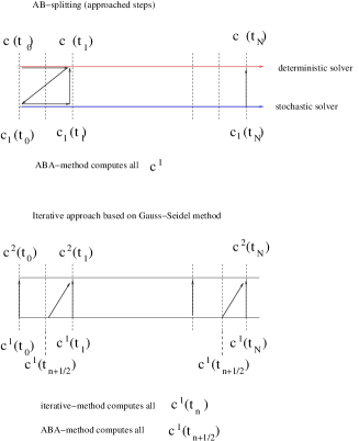
Figure 3: The improvements with the iterative approaches with the help of the AB- and ABA splitting approach.

4 Numerical Analysis

In the numerical analysis, we concentrate on the new iterative algorithms and present the approximation to the fixpoint of the solutions.

The iterative splitting scheme is given as:

$$\frac{\partial c_{i}}{\partial t}dt=-\frac{\partial f(c_{i-1},c_{i})}{\partial x}+\sigma(c_{i-1}(t))\;dW_{t},\;c_{i}(x,t^{n})=c(x,t^{n}),$$ (49)

where we have $i=1,2,\ldots,I$ with the start condition $c_{0}(t)=c(t^{n})$.

We apply the integration and have the solution

$$\int_{t^{n}}^{t^{n+1}}\frac{\partial c_{i}}{\partial t}dt=-\int_{t^{n}}^{t^{n+1}}\frac{\partial f(c_{i-1},c_{i})}{\partial x}+\int_{t^{n}}^{t^{n+1}}\sigma(c_{i-1}(t))\;dW_{t},\;c_{i}(x,t^{n})=c(x,t^{n}),$$

$$c_{i}(t^{n+1})=S_{Burgers}(\Delta t,c_{i-1}(t^{n}))\;c(t^{n})+$$

$$+\int_{t^{n}}^{t^{n+1}}S_{Burgers}(t^{n+1}-s,c_{i-1}(t^{n+1}-s))\;\sigma(c_{i-1}(s))\;dW_{s},$$ (50)

with initialization $c_{0}(t)=c(t^{n})$ and $i=1,\ldots,I$.

Definition 1

We have $\Omega\subset{\rm I}\!{\rm R}^{N}$ and $G:\Omega\rightarrow{\rm I}\!{\rm R}^{M}$. Further, $G$ is Lipschitz contiuous on $\Omega$ with Lipschitz-constant $\gamma$ if

$$||G(x)-G(y)||\leq\gamma||x-y||,$$ (51)

for all $x,y\in\Omega$.

We have the following assuptions:

Assumption 4.1

We have the Lipschitz-constinuous functions $S_{b}(c)$ and $\sigma(c)$, while we also assume $\frac{\partial\sigma}{\partial c}$ is Lipschitz continuous.

Then, we have the following Lemma:

Lemma 1

We have $\Omega\subset{\rm I}\!{\rm R}^{N}$ and $S_{b},\frac{\partial\sigma}{\partial c}:\Omega\rightarrow{\rm I}\!{\rm R}^{M}$. Further, $S_{b}$ and $\frac{\partial\sigma}{\partial c}$ are contraction mappings on $\Omega$, while we assume $\frac{\partial\sigma}{\partial c}$ are Lipschitz continuous with constants $\gamma_{1}\leq 1$ and $\gamma_{2}\leq 1$.

Proof

We have

$$||S_{b}(x^{n})x-S_{b}(y^{n})y||\leq\gamma_{1}||x-y||,$$ (52)

While the operator $S_{b}$ for the pure deterministic Burgers’ equation is bounded with respect to $\Delta x$ and $\Delta t$ we obtain $||S_{b}(x^{n})||\leq\gamma_{1}$ for sufficient small $\Delta x$ and $\Delta t$.

Further, we have

$$||\frac{\partial\sigma}{\partial x}|_{x=x^{n}}x-\frac{\partial\sigma}{\partial y}|_{y=y^{n}}y||\leq\gamma_{2}||x-y||,$$ (53)

while the operator $\frac{\partial\sigma}{\partial x}$ is bounded and lipschitz continuous.

Theorem 4.2

$\Omega$ is a closed subset of ${\rm I}\!{\rm R}^{N}$ and $S_{B}$ and $\frac{\partial\sigma}{\partial x}$ are contraction mappings on $\Omega$ with Lipschitz-constants $\gamma_{1}<1$ and $\gamma_{2}<1$, then the iterative scheme (4) converge linearly to $x^{*}$ with the factor $\tilde{\gamma}$.

Proof

We apply the iterative scheme:

$$\int_{t^{n}}^{t^{n+1}}\frac{\partial c_{i}}{\partial t}dt=-\int_{t^{n}}^{t^{n+1}}\frac{\partial f(c_{i-1},c_{i})}{\partial x}+\int_{t^{n}}^{t^{n+1}}\sigma(c_{i-1}(t))\;dW_{t},\;c_{i}(x,t^{n})=c(x,t^{n}),$$

$$c_{i}(t^{n+1})=S_{Burgers}(\Delta t,c_{i-1}(t^{n}))\;c(t^{n})+$$

$$+\int_{t^{n}}^{t^{n+1}}S_{Burgers}(t^{n+1}-s,c_{i-1}(t^{n+1}-s))\;\sigma(c_{i-1}(s))\;dW_{s},$$ (54)

and evalutate the integral based on the Taylor-Ito scheme at the integration point $t^{n}$ and obtain, accuracy of the Milstein-scheme, which is given as:

$$c_{i}(t^{n+1})=S_{Burgers}(\Delta t,c_{i-1}(t^{n}))c(t^{n})+$$ (55)

$$+S_{Burgers}(\Delta t,c_{i-1}(t^{n}))\sigma(c(t^{n}))\;\Delta W_{t^{n+1}}+$$

$$+\frac{1}{2}\left(S_{Burgers}(\Delta t,c_{i-1}(t^{n}))\right)^{2}\sigma(c(t^{n}))\left(\frac{\partial\left(\sigma(c)\right)}{\partial c}\right)|_{c_{i-1}(t^{n})}(\Delta W_{t^{n+1}}^{2}-\Delta t).$$

We apply:

$$||c_{i}(t^{n+1})-c_{i-1}(t^{n+1})||\leq$$

$$\leq||S_{Burgers}(\Delta t,c_{i-1}(t^{n}))-S_{Burgers}(\Delta t,c_{i-2}(t^{n}))||||c(t^{n})||+$$

$$||S_{Burgers}(\Delta t,c_{i-1}(t^{n}))-S_{Burgers}(\Delta t,c_{i-2}(t^{n}))||||\sigma(c(t^{n}))\;\Delta W_{t^{n+1}}||+$$

$$+\frac{1}{2}||\left(S_{Burgers}(\Delta t,c_{i-1}(t^{n}))\right)^{2}\left(\frac{\partial\left(\sigma(c)\right)}{\partial c}\right)|_{c_{i-1}(t^{n})}-$$

$$-\left(S_{Burgers}(\Delta t,c_{i-2}(t^{n}))\right)^{2}\left(\frac{\partial\left(\sigma(c)\right)}{\partial c}\right)|_{c_{i-2}(t^{n})}||\cdot$$

$$\cdot||\sigma(c(t^{n}))\;(\Delta W_{t^{n+1}}^{2}-\Delta t)||\leq$$

$$\leq\gamma_{1}||c_{i-1}(t^{n})-c_{i-2}(t^{n})||C_{1}+\gamma_{1}||c_{i-1}(t^{n})-c_{i-2}(t^{n})||C_{2}+$$

$$+\gamma_{1}\gamma_{2}||c_{i-1}(t^{n})-c_{i-2}(t^{n})||C_{3}\leq$$

$$\leq\tilde{\gamma}||c_{i-1}(t^{n})-c_{i-2}(t^{n})||\tilde{C},$$ (56)

where we assume the constants $C_{1},C_{2},C_{3}$ and $\tilde{C}$ are bounded and $\tilde{\gamma}<1$ with sufficient small $\Delta t$ and $\Delta x$.

We apply the recursion and obtain:

$$||c_{i}(t^{n+1})-c_{i-1}(t^{n+1})||\leq\tilde{\gamma}^{i}||c_{i-1}(t^{n+1-i})-c_{i-2}(t^{n+1-i})||\tilde{C}^{i},$$ (57)

where we obtain $\lim_{n,i\rightarrow\infty}||c_{i}(t^{n+1})-c_{i-1}(t^{n+1})||\rightarrow 0$.

Remark 1

We obtain a convergence to the fixpoint of the equation based on the iterative scheme. We also obtain an acceleration of the solver-process and a reduction of the numerical error with additional iterative steps.

4.1 Numerical Error Analysis (strong and weak errors)

For the verification of the theoretical results for the iterative splitting scheme in section 3, we deal with the following numerical error analysis.

We present the convergence rates of the following weak errors:

• Weak errors:

  $$err_{weak,\Delta t}=|E(c_{\Delta t,Scheme})-c_{\Delta t,pureburg})|,$$

  $$=\left|\left(\frac{1}{N}\sum_{j=1}^{N}c_{\Delta t,Scheme,j}\right)-c_{\Delta t,pureburg}\right|,$$ (58)

  where $N$ are the number of solutions of the stochastic Burgers’ equation.

  Further $c_{\Delta t,pureburg}$ is the solution of the pure Burgers’ equation and $c_{\Delta t,Scheme,j}$ is the $j$-th solution of the stochastic Burgers’ equation. We assume to have $10-100$ runs of the stochastic Burgers’ equation.

• Variance for the solution at $t=t_{n}$ and $N_{s}$-sample paths:

  $$Var(c_{\Delta t,Scheme}(t_{n}))=E(\left(c_{\Delta t,Scheme}(t_{n})-E(c_{\Delta t,Scheme}(t_{n}))\right)^{2})=$$

  $$=\left(\frac{1}{N}\sum_{j=1}^{N}(c_{\Delta t,Scheme}(t_{n}))^{2}\right)-E(c_{\Delta t,Scheme,j}(t_{n})),$$ (59)

  we deal with $N_{s}$ number of seeds and $method=\{AB,ABA,BAB,iter\}$, $c_{\Delta t,Scheme,j}$ is the result of the method at $t^{n}$ in the seed $j$. Further, we apply for the iterative scheme $iter=1,\ldots,iter=4$ steps.

Remark 2

In the numerical examples, we obtain the weak convergence rates with the weak error. Here, we also apply the weak error to obtain an overview to the accuracy of the numerical schemes.

5 Numerical experiments

In the following numerical experiments, we concentrate on pure stochastic Burgers’ equation, which is given as:

$$\frac{\partial c}{\partial t}+\frac{\partial f(c)}{\partial x}=\sigma(c)\frac{\partial W}{\partial t},\;(x,t)\in[0,X]\times[0,T],$$ (60)

$$c(x,0)=c_{0}(x),\;x\in[0,X].$$ (61)

For the discretization with Finite Difference or Finite Volumes, we deal with the CFL condition of the two explicit discretized terms as:

• $\Delta t\leq\frac{\Delta x}{|u_{i}^{n-1}|}$, for the deterministic part,

• $\Delta t\leq\frac{(u_{i}^{n-1})^{2}}{(\sigma(u_{i}^{n-1}))^{2}\xi^{2}}$, for the stochastic part,

• $\Delta t\leq\left(\frac{1}{\frac{|u_{i}^{n-1}|}{\Delta x}+\frac{\sigma(u_{i}^{n-1})|\xi|}{u_{i}^{n-1}}}\right)^{2}$, for both terms and we assume $\sqrt{\Delta t}\leq\Delta t$ ,

where we use estimates for $u_{i}^{n-1}$ and $\Delta W=\sqrt{\Delta t}\;\xi$ with $\xi$ is Gaussian normal distributed.

We apply the following methods, that we discussed in section 3:

• AB-splitting,

• ABA-splitting,

• BAB-splitting,

• iter-splitting (where we apply $i=1,\ldots,4$ iterative steps).

The $L_{1}$-errors of the different numerical schemes are given in figure 4.

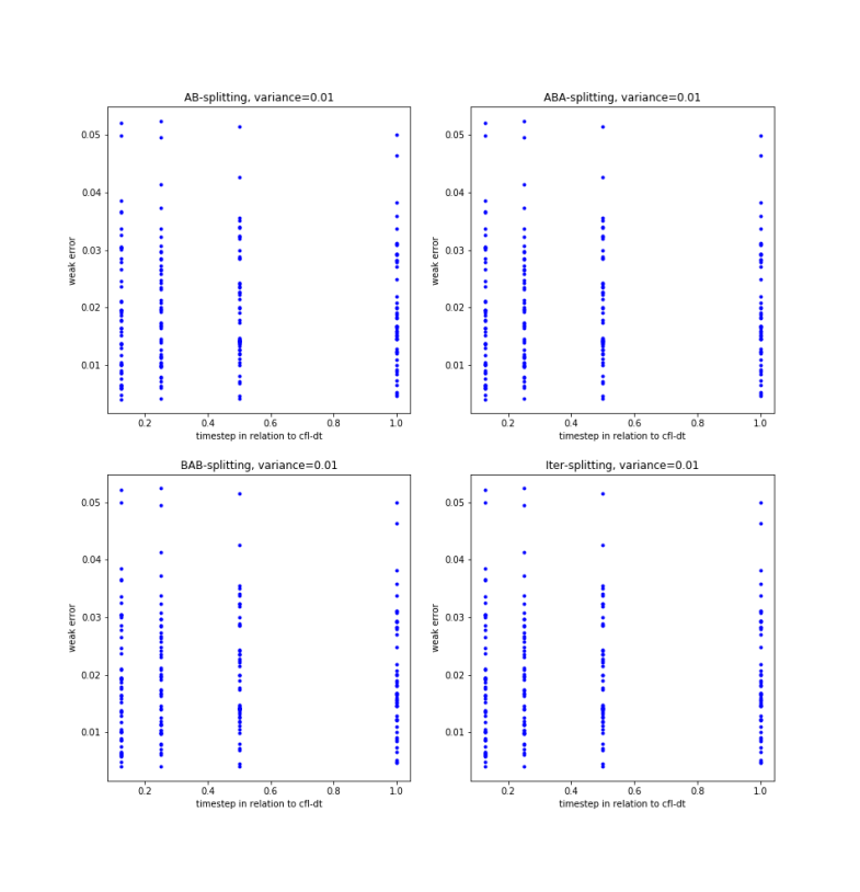
Figure 4: Left upper figure: $L1$-errors of the AB-spitting approach, right upper figure: $L1$-errors of the ABA-spitting approach, left lower figure: $L1$-errors of the BAB-spitting approach and right lower figure: $L1$-errors of the itertative-spitting approach.

The comparison of the schemes with the iterative splitting approach is given in figure 5.

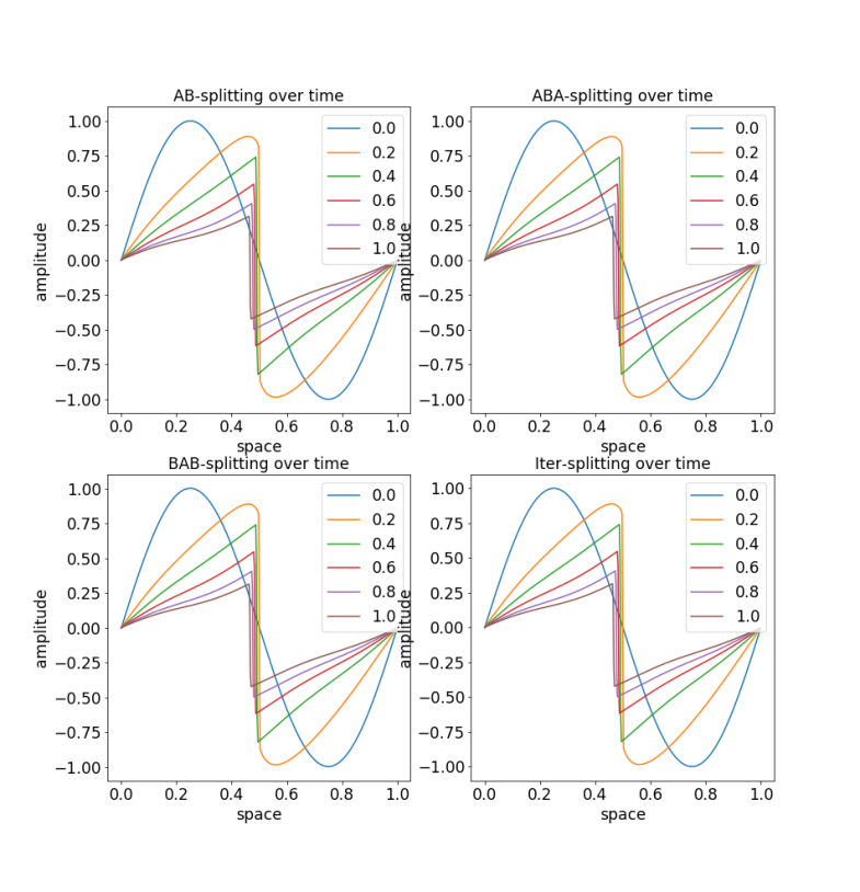
Figure 5: Simulation-results of the different methods and the improved iterated approaches.

The $L1$ errors are defined as errors to compare to the weak and strong convergence, while $err_{weak}$ is defined to see the error of the averaged stochastic solution to the deterministic solution. The errors of the schemes are presented in figure 6.

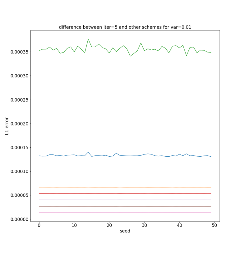
Figure 6: $L_{1}$-error of the simulation-results of the different methods with different iterative steps.

The seeds and the blow-ups of the noniterative splitting approaches are presented in 7. For the experiments and the numerical tests, we initialize the pseudo random generator for each new perturbation with a new seed.

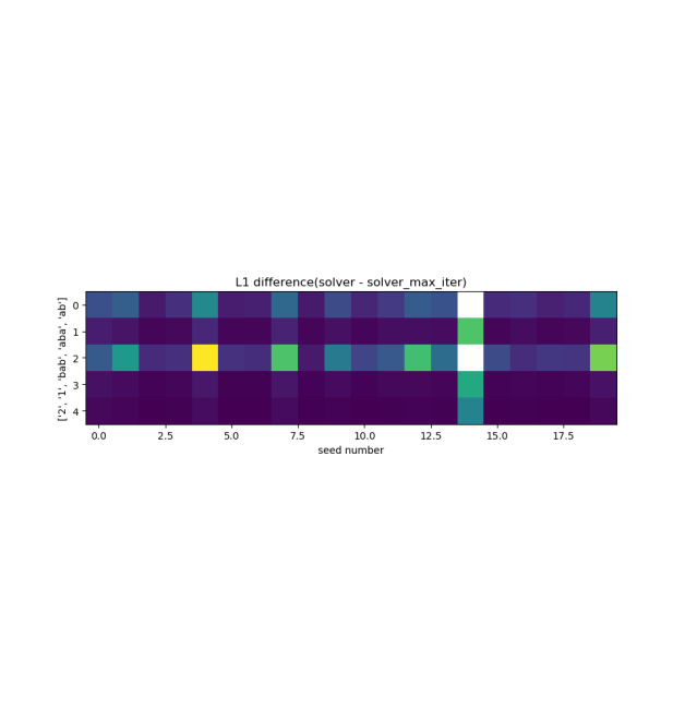
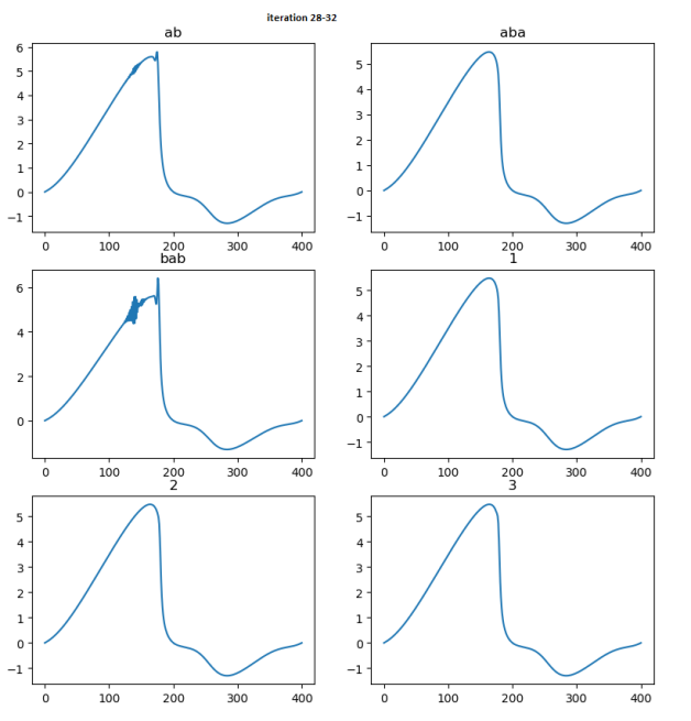
Figure 7: In the left figure, we see the different seeds of the non-iterative and iterative approaches. The right figure presents the benefits of the iterative approaches, while in the non-iterative approaches, we have blow-up.

The numerical errors between the perturbed and unperturbed solution and the averaged results are given in figure 8.

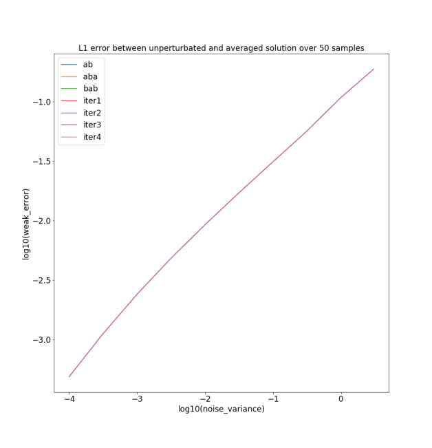
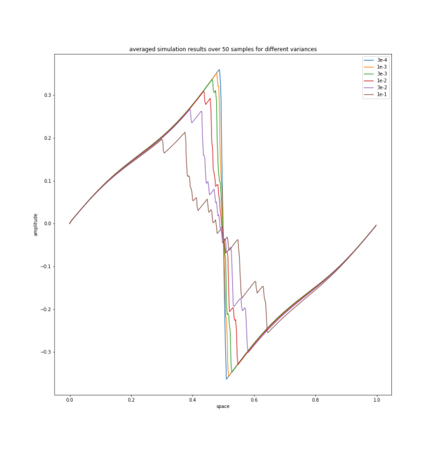
Figure 8: In the left figure, we see $L_{1}$ error between unperturbated solution and average over $50$ perturbed solutions, only AB-splitting, dependent on variances. The right figure presents the averaged results for difference variances.

Remark 3

With the iterative splitting schemes, we obtain more accurate results and reduce the numerical errors in each iterative step.

6 Conclusion

We presented new iterative methods based on the Picard’s approximation. Such methods allow to obtain more accurate results, while we could reduce the error with the iterative steps. We presented first numerical results with the stochastic Burgers’ equation and multiplicative noise. In future, we also apply more delicate SPDEs with respect to mixed time and spatial noises.

7 Appendix

In the following, we add some more details to the iterative and non-iterative schemes.

7.1 Derivations of the methods

The SDE is given as:

$$u(x,t)_{t}+0.5(u(x,t)^{2})_{x} =\sigma(u(x,t))W(t)_{t}$$ (62)

$$u_{t}+0.5(u^{2})_{x} =\sigma(u)W_{t},$$

$u=u(x,t)$ is a spatial dependent amplitude, that changes over time. $W=W(t)$ is a Wiener process (Standard Brownian motion, summation of white noise) over time and $W_{t}$ is its time derivative; so basically white noise. $\sigma(u,t)$ is the diffusion coefficient and can further be time variant or dependent on past values of $u$. For the sake of brevity, some variables stay omitted.

Ignoring the stochastic part on the right, one can transform the deterministic part and match it against the standard Burgers’ equation (missing diffusion term $v=0$ in this case),

$$u_{t}+0.5\frac{\partial}{\partial x}(u^{2})=u_{t}+uu_{x} =0$$ (63)

$$u_{t}+uu_{x} =v\frac{\partial^{2}u}{\partial x^{2}}$$

which is solved on a discrete time grid by the conservation law solver with Engquist-Osher in the function $SCL$ (solve conservation law).

A stochastic equation of the form

$$dX_{t}=\mu Xdt+\sigma XdW_{t}$$ (64)

with real constants $\mu$ and $\sigma$ can be solved by the Milstein method and has the numerical solution

$$X_{t+\Delta t}=X_{t}+a(X_{t})\Delta t+b(X_{t})\Delta W_{t}+\frac{1}{2}b(X_{t})b^{\prime}(X_{t})((\Delta W_{t})^{2}-\Delta t)$$ (65)

with drift $a(x)=\mu x$ and diffusion $b(x)=\sigma x$. Via pattern matching, one can deduce a numerical solution for the stochastic part:

$$u_{t+\Delta t} =u_{t}+\sigma(u_{t})W_{t}$$ (66)

$$u_{t+\Delta t} =u_{t}+\sigma(u_{t})\Delta W_{t}+\frac{1}{2}\sigma(u_{t})\sigma^{\prime}(u_{t})((\Delta W_{t})^{2}-\Delta t).$$

Note that the notation of an index like _t may refer to a derivative in continuous time or time stamp in discrete time. This solver is implemented in the function $SSDE$ (solve stochastic differential equation).

7.2 AB-splitting

The AB-splitting approach divides the time scale into $N$ intervals. Each interval is further split into $J$ subintervals. The AB-splitting takes an initial condition $u(t)$ and solves the deterministic problem on the subinterval $J$ to obtain a solution $u(t+\Delta t)_{1}$. The deterministic result is used as initial condition for the stochastic solver, which calculates the final result $u(t+\Delta t)$. This process is repeated $N$ times to obtain the final result.

7.3 ABA-splitting

This algorithm works almost identically to the upper one, but with a slight modification with regards to the order and length of the solvers. The deterministic solver is used on the first half of the subinterval, resulting in a helper solution $u(t+\frac{1}{2}\Delta t)_{1}$. The stochastic solver than proceeds to calculate a solution on the whole subinterval and yields another solution $u(t+\Delta t)_{2}$, which is used as initial condition for the deterministic solver in order to yield the final result $u(t+\Delta t)$ for the second half of the subinterval.

7.4 BAB-splitting

The same as above, but stochastic and deterministic solver are exchanged.

7.5 iterative splitting (after discretization)

The iterative scheme, here we apply the iterative steps of a stochastic equation of the form

$$dX_{i,t}=a(X)dt+b(X)dW_{t}$$ (67)

while we obtain an analytical solution of $dX_{i,t}=a(X_{i})dt$, which is $X_{t+\Delta t}=S(a(X_{t}),\Delta t)X_{t}$.

We apply the Milstein-scheme plus a fixpoint iterative scheme, which is given as

$$X_{i}(t^{n+1})=S_{Burgers}(\Delta t,a(X_{i-1}^{n+1}))X^{n}+b(X_{i-1}^{n+1})\Delta W+$$

$$+b(X_{i-1}^{n+1})\frac{\partial b(X)}{\partial X}|_{X=X_{i-1}^{n+1}}(\Delta W^{2}-\Delta t),$$ (68)

with drift $a(x)$ and diffusion $b(x)$.

7.6 iterative splitting (before discretization)

iterative Steps $i>1$):

$$c_{i}(t^{n+1})=S_{Burgers}(\Delta t,c(t^{n}))c(t^{n})+S_{Burgers}(\Delta t,c(t^{n}))\sigma(c_{i-1}(t^{n+1}))\;\Delta W_{t^{n+1}}+$$ (69)

$$+\frac{1}{2}\left(S_{Burgers}(\Delta t,c(t^{n}))\right)^{2}\sigma(c_{i-1}(t^{n+1}))\left(\frac{\partial\left(\sigma(c)\right)}{\partial c}\right)|_{c_{i-1}(t^{n+1})}(\Delta W_{t^{n+1}}^{2}-\Delta t),$$

7.7 Improvements be the integration of the variation of constants

$i=2$ (trapezoidal rule):

$$c_{2}(t^{n+1})=S_{Burgers}(\Delta t)c(t^{n})-$$

$$-\frac{1}{2}\sigma(c_{1}(t^{n+1}))^{2}\;\Delta t+\sigma(\frac{c_{1}(t^{n+1})+c(t^{n})}{2})\;\Delta W_{t}.$$ (70)

$i>2$:

$$c_{i}(t^{n+1})=S_{Burgers}(\Delta t)c(t^{n})-$$

$$-\frac{1}{2}\sigma(c_{1}(t^{n+1}))^{2}\;\Delta t+\sigma(\frac{c_{i-1}(t^{n+1})+c(t^{n})}{2})\;\Delta W_{t}.$$ (71)

with $i=3,\ldots,I$.

7.8 Numerical Errors: Weak and Strong error

• Strong error:

  $${L_{1}}_{strong,\Delta t,\Delta x,s}=E(|U_{ref}-U_{scheme}|)=$$

  $$=\sum_{s=1}^{N_{s}}(\sum_{j=1}^{N}|u_{\Delta t,\Delta x,j,reference,s}-u_{\Delta t,\Delta x,j,scheme,s}|/N)/N_{s},$$ (72)

  where $s$ is the index of the different seeds, meaning $W(s)$ (different Wiener-processes) and $N=N_{t}\cdot N_{x}$ is the number of the $N_{t}$ temporal and $N_{x}$ spatial steps. Furthermore $reference$ is the deterministic reference solution and we test the schemes $scheme=\{AB,\;ABA,\;BAB,\;iter\}$.

• Weak error:

  $${L_{1}}_{weak,\Delta t,\Delta x,s}=|E(f(U_{ref})-E(f(U_{scheme}))|=$$ (73)

  $$=|\sum_{s=1}^{N_{s}}(\sum_{j=1}^{N}u_{\Delta t,\Delta x,j,reference,s}/N)/N_{s}-\sum_{s=1}^{N_{s}}(\sum_{j=1}^{N}u_{\Delta t,\Delta x,i,scheme,s}/N)/N_{s}|,$$

  where we assume $f(u)=u$, further $s$ is the index of the different seeds for $W(s)$ (different Wiener-processes) and $N_{s}$ are the number of seeds. $N=N_{t}\cdot N_{x}$ is the number of the $N_{t}$ temporal and $N_{x}$ spatial steps. Additionally $reference$ is the deterministic reference solution and we test the schemes $scheme=\{AB,\;ABA,\;BAB,\;iter\}$. The weak error is defined with the average value of the stochastic result, while the reference solution is the deterministic result.

References

• [1] M. Beccari, M. Hutzenthaler, A. Jentzen, R. Kurniawan, F. Lindner and D. Salimova. Strong and weak divergence of exponential and linear-implicit Euler approximations for stochastic partial differential equations with superlinearly growing nonlinearities. arXiv e-prints, arXiv:1903.06066, 2019.
• [2] J.R. Beddington and R.M. May. Harvesting natural populations in a randomly fluctuating environment. Science, 197(4302):463-465, 1977.
• [3] D. Blömker. Amplitude Equations for Stochastic Partial Differential Equations. Interdisciplinary Mathematical Sciences (cvol. 3), World Scientific Publishing Co. Pte. Ltd., Hackensack, NJ, 2007.
• [4] B. Birnir. The Kolmogorov-Obukhov Theory of Turbulence: A mathematical theory of turbulence. Springer Briefs in Mathematics. Springer, New York, 2013.
• [5] L.C. Evans. An Introduction to Stochastic Differential Equations. American Mathematical Society, 2013.
• [6] J. Geiser. Iterative Splitting Methods for Differential Equations. CRC Press, Taylor & Francis, Boca Raton, London, New York, 2011.
• [7] J. Geiser. Multicomponent and Multiscale Systems—Theory, Methods, and Applications in Engineering. Springer-Verlag, Berlin, 2016.
• [8] J. Geiser. Iterative Semi-implicit Splitting Methods for Stochastic Chemical Kinetics. Finite Difference Methods: Theory and Applications, Springer International Publishing, Cham, 35-47, 2019.
• [9] M. Hairer and J. Voss. Approximations to the Stochastic Burgers Equation. Journal of Nonlinear Science, 21(6):897-920, 2011.
• [10] A. Harten, S. Osher, B. Engquist, and S.R. Chakravarthy. Some results on uniformly high-order accurateessentially nonoscillatory schemes. Appl. Numer. Math., 2(3-5):347-378, 1986.
• [11] H. Holden and N.H. Risebro. Front Tracking for Hyperbolic Conservation Laws. Springer-Verlag Berlin Heidelberg, second edition edition, 2015.
• [12] T. Iliescu, H. Liu and X. Xie. Regularized reduced order Models for a Stochastic Burgers Equation. International Journal of Numerical Analysis and Modelling, 15(4-5):594-607, 2018.
• [13] K.H. Karlsen and E.B. Storrosten. Analysis of a splitting method for stochastic balance laws. IMA Journal of Numerical Analysis, 38, 1-56, 2018.
• [14] K.H. Karlsen, E.B. Storrosten. On stochastic conservation laws and Malliavin calculus. Journal of Functional Analysis, 272: 421-497, 2017.
• [15] P.E. Kloeden and E. Platen. The Numerical Solution of Stochastic Differential Equations. Springer-Verlag, Berlin, 1992.
• [16] M. A. Munoz. Multiplicative noise in non-equilibrium phase transitions: A tutorial. In Advances in Condensed Matter and Statistical Physics, pages 37–68. Nova Science Publishers, Inc., 2004.
• [17] S. Ninomiya and N. Victoir. Weak approximation of stochastic differential equations and application to derivative pricing. Appl. Math. Finance, 15:107-121, 2008.
• [18] B. Oksendal. Stochastic Differential Equations: An Introduction with Applications. Springer-Verlag, Berlin, 2002.
• [19] A. Rösequential splittingler. Runge–Kutta Methods for Itô Stochastic Differential Equations with Scalar Noise. BIT Numerical Mathematics, 46(1):97-110, 2006.
• [20] G. Strang. On the construction and comparison of difference schemes. SIAM J. Numer. Anal. 5:506–517, 1968.
• [21] H.F. Trotter. On the product of semi-groups of operators. Proceedings of the American Mathematical Society 10(4):545–551, 1959.