Decorrelated Local Linear Estimator: Inference for Non-linear Effects in High-dimensional Additive Models

Abstract

Additive models play an essential role in studying non-linear relationships. Despite many recent advances in estimation, there is a lack of methods and theories for inference in high-dimensional additive models, including confidence interval construction and hypothesis testing. Motivated by inference for non-linear treatment effects, we consider the high-dimensional additive model and make inference for the derivative of the function of interest. We propose a novel decorrelated local linear estimator and establish its asymptotic normality. The main novelty is the construction of the decorrelation weights, which is instrumental in reducing the error inherited from estimating the nuisance functions in the high-dimensional additive model. We construct the confidence interval for the function derivative and conduct the related hypothesis testing. We demonstrate our proposed method over large-scale simulation studies and apply it to identify non-linear effects in the motif regression problem. Our proposed method is implemented in the R package DLL available from CRAN.

1 Introduction

Additive models play an important role in modern data analysis [8, 55, 29]. The additive model is useful as it relaxes the stringent linearity assumption imposed in the multiple linear models and generalizes the nice interpretation of linear models. In the low-dimensional setting, additive models have been carefully investigated [8, 55, 29, 42, 32, 39, e.g.]. Recently, there has been a growing interest in the high-dimensional additive model, which generalizes the high-dimensional linear regression. Much progress has been made to understand the prediction performance of various proposals, including [40, 37, 46, 51, 52, 57, 58, 47]. However, the statistical inference problem in the high-dimensional additive model is far less understood from both methodological and theoretical perspectives.

Statistical inference in high-dimensional additive models is well-motivated from causal inference with observational studies. Causal conclusions from observational studies are invalidated due to unmeasured confounders [33, 43, e.g.]. A commonly used approach is to condition on a large number of measured covariates such that the conditional ignorability condition holds [4, 31, e.g.]. This idea has been carefully investigated by utilizing high-dimensional linear models. However, the linear model imposes a stringent assumption that the exposure has a constant effect on the outcome regardless of the exposure value. Such an assumption might not be plausible for various applications; see the application to motif regression in Section 5 for example. Non-linear effects have been commonly observed in scientific studies, including return to schooling [13], climate on crop yields [49], and the climate change on the economic outcomes [20, 19]. The additive model significantly relaxes the linearity assumption and better accommodates the possibly non-linear effect.

In this paper, we consider the additive model for the outcome variable $Y_{i}\in\mathbb{R}$,

$$Y_{i}=f(D_{i})+g(X_{i})+\epsilon_{i}\quad\text{with}\quad g(X_{i})=\sum_{j=1}^{p}g_{j}(X_{i,j}),\quad\text{for}\quad 1\leq i\leq n,$$ (1)

where $D_{i}\in\mathbb{R}$ is the variable of interest (e.g. the exposure or treatment variable), $X_{i}\in\mathbb{R}^{p}$ is the high-dimensional baseline covariates, $\mathbf{E}(\epsilon_{i}\mid D_{i},X_{i})=0,$ and $f:\mathbb{R}\rightarrow\mathbb{R}$ and $g_{j}:\mathbb{R}\rightarrow\mathbb{R}$ for $1\leq j\leq p$ are unknown functions. The observed data $\{Y_{i},D_{i},X_{i}\}_{1\leq i\leq n}$ are assumed to be independently and identically distributed. For a pre-specified $a_{0}\in\mathbb{R}$ and a small $\tau>0,$ the ratio $\left(f(a_{0}+\tau)-f(a_{0})\right)/\tau$ captures the exposure’s effect at $a_{0}$. With $\tau$ approaching zero, the function derivative $f^{\prime}(a_{0})$ measures the exposure’s effect on the outcome [3]. The current paper is focused on statistical inference for $f^{\prime}(a_{0})$ with $a_{0}\in\mathbb{R}$ under the high-dimensional additive model (1).

1.1 Results and contributions

In the univariate setting, the local linear estimator is the state-of-the-art method to make inference for $f^{\prime}(a_{0})$ [23, 22, e.g.]. However, the inference problem under the high-dimensional additive model (1) is much more challenging due to the presence of the unknown high-dimensional function $g$. With an accurate estimator $\widehat{g}$, the estimated variables $\widehat{Y}_{i}=Y_{i}-\widehat{g}(X_{i})$ for $1\leq i\leq n$ can be used as proxies for $\{f(D_{i})\}_{1\leq i\leq n}$. A natural idea is to estimate $f^{\prime}(a_{0})$ by applying the local linear method to $\{D_{i},\widehat{Y}_{i}\}_{1\leq i\leq n}$ with $\{\widehat{Y}_{i}\}_{1\leq i\leq n}$ as the outcome variables. However, such a plug-in estimator suffers from large estimation bias due to the estimation error of $\widehat{g}$; see Table 1 in Section 4.1 for illustrations.

We propose a novel Decorrelated Local Linear (DLL) estimator of $f^{\prime}(a_{0}).$ The classical local linear estimator can be expressed as a weighted average of the outcome variables, where the local linear kernel induces the weights. As the major novelty, we construct the decorrelation weights to mitigate the error inherited from the high-dimensional estimator $\widehat{g}$. Meanwhile, the constructed decorrelation weights ensure that the standard error of our proposed DLL estimator is comparable to that of the classical local linear estimator. The decorrelation weights are constructed in a non-parametric way and designed for the bias correction of the local linear estimator.

In Theorem 1, we establish the asymptotic normality of our proposed DLL estimator as long as the estimator $\widehat{g}$ is consistent. We further show that the asymptotic variance of our proposed estimator matches with the optimal rate in the univariate setting [23]. We construct the confidence interval for $f^{\prime}(a_{0})$ and test for the hypothesis $H_{0}:f^{\prime}(a_{0})=0$.

In Section 4, we demonstrate the validity of our theoretical results in moderate sample sizes, address practical issues on algorithm implementation, and provide practical recommendations. Our proposed method is implemented in the R package DLL, which is available from CRAN. The simulation results show that the DLL estimator significantly outperforms the plug-in estimator and the ReSmoothing estimator [27], in terms of the bias correction and coverage property. Regarding the empirical coverage and length, the confidence intervals (CIs) based on the DLL estimator are comparable to the oracle CIs, which are constructed with the oracle knowledge of the high-dimensional function $g$.

In Section 5, we conduct a careful analysis of the motif regression problem [59] and observe a highly non-linear relationship between the gene expression level and the motif scores. Our results demonstrate the advantage of our proposed method over the statistical inference method assuming the linear outcome model.

1.2 Literature review and comparison

Two recent works [27] and [38] studied the inference problems in high-dimensional additive models. Specifically, [27] proposed a two-step ReSmoothing (RS) estimator: in the first step, a pre-smoothing estimator was obtained; in the second step, the pre-smoothing estimator was taken as the proxy outcome, and standard univariate non-parametric technique was then applied. In Section 4.2, we compare our proposed DLL estimator with the RS estimator and observe that the RS estimator suffers from a large bias of estimating the function derivative while our proposed DLL estimator corrects the bias effectively. Consequently, our proposed confidence interval has better empirical coverage than that based on the RS estimator; see Table 3 for the detailed comparison. In addition, [38] considered the confidence band construction problem under the high-dimensional sparse additive model, which is a different inference problem from the current paper.

Inference for function derivative has been actively studied in the non-parametric modeling, including local linear estimator [22], regression spline [61], kernel methods [26], empirical likelihood methods [44], and others cited therein. However, as discussed, the unknown high-dimensional function $g$ in the additive model poses great challenges to statistical inference for the function derivative at a local point. The paper [3] studied the inference for the function derivative in additive models without the sparsity structure. The penalty is essential to recovering the high-dimensional sparse model, which creates an additional bias to correct in the following inference step. The statistical inference problem with the sparsity structure requires extra innovation in terms of both method and theory.

A recent line of active research was focused on statistical inference in high-dimensional linear regression. Debiased estimators or Neyman’s Orthogonalization were proposed for inference for single regression coefficients [60, 54, 34, 5, 15, 24, 14]. The linear model is a special case of the additive model, where the function derivative $f^{\prime}(a_{0})$ is assumed to be a constant for any $a_{0}\in\mathbb{R}$. Statistical inference for the non-linear effect in the additive model is a much more challenging problem, which requires novel methods and theories to address the non-linearity. Both the rate of convergence and the sufficient conditions for confidence interval construction are different from those established in the high-dimensional linear regression. A more detailed methodological comparison is presented in Remark 2. The real data analysis in Section 5 shows that a misleading scientific conclusion might be obtained without accounting for the possible non-linear effects.

Beyond the high-dimensional linear regression, [14] and [63] studied the inference procedure for the partially linear model. However, the focus is still on the inference problem for the linear component instead of the non-linear component addressed here.

Organization. In Section 2, we introduce the decorrelated local linear estimator. In Section 3, we establish the theoretical guarantee of the proposed estimator. In Section 4, we conduct a large-scale simulation study to demonstrate the finite-sample performance of the DLL estimator. In Section 5, we apply the DLL estimator to the motif regression problem. In Section 6, we provide conclusion and discussion.

Notations. For a sequence of random variables $X_{n}$ indexed by $n$, we use $X_{n}\overset{p}{\to}X$ and $X_{n}\overset{d}{\to}X$ to represent that $X_{n}$ converges to $X$ in probability and in distribution, respectively. For a matrix $X$, we use $X_{i,j}$, $X_{i}$, and $X_{\cdot,j}$ to denote its $(i,j)$ entry, the $i$-th row and $j$-th column, respectively; for index sets $S_{1}$ and $S_{2}$, $X_{S_{1},S_{2}}$ denotes the sub-matrix of $X$ with row and column indices belonging to $S_{1}$ and $S_{2}$, respectively. We use $c$ and $C$ to denote generic positive constants that may vary from place to place. For two positive sequences $a_{n}$ and $b_{n}$, $a_{n}\lesssim b_{n}$ means $a_{n}\leq Cb_{n}$ for all $n$ and $a_{n}\gtrsim b_{n}$ if $b_{n}\lesssim a_{n}$ and $a_{n}\asymp b_{n}$ if $a_{n}\lesssim b_{n}$ and $b_{n}\lesssim a_{n}$, and $a_{n}\ll b_{n}$ if $\limsup_{n\rightarrow\infty}{a_{n}}/{b_{n}}=0$ and $a_{n}\gg b_{n}$ if $b_{n}\ll a_{n}$.

2 Decorrelated local linear estimator

We consider the data $\{X_{i},D_{i},Y_{i}\}_{1\leq i\leq n}$ being i.i.d. generated, where for the $i$-th subject, $Y_{i}\in\mathbb{R}$ denotes the outcome variable, $D_{i}\in\mathbb{R}$ denotes the variable of interest, and $X_{i}\in\mathbb{R}^{p}$ denotes the high-dimensional baseline covariates. We focus on the additive outcome model (1). Our goal is to make inference for the function derivative $f^{\prime}(a_{0})$ with $a_{0}\in\mathbb{R}$ denoting a pre-specified value belonging to the range of $D_{i}.$

2.1 Decorrelation for the local linear estimator

The local polynomial estimator [22, 50, 16, 21] has been developed under the univariate non-parametric regression $Y_{i}=f(D_{i})+\epsilon_{i},$ for $1\leq i\leq n,$ with $f:\mathbb{R}\rightarrow\mathbb{R}$ denoting an unknown smooth function. By the Taylor expansion $f(D_{i})=f(a_{0})+{f^{\prime}}(a_{0})(D_{i}-a_{0})+r(D_{i})$ for $a_{0}-h\leq D_{i}\leq a_{0}+h,$ we approximate $f$ by a linear function in a small neighborhood of $a_{0}$ and estimate $f^{\prime}(a_{0})$ by fitting a linear model within this small neighborhood. For a pre-specified bandwidth $h>0$, define the kernel

$$K_{h}(d)=\frac{1}{2h}\cdot\mathbf{1}\left(|D_{i}-a_{0}|\leq h\right).$$ (2)

The local linear estimator of $f^{\prime}(a_{0})$ has the following explicit form,

$$\frac{\sum_{i=1}^{n}W^{0}_{i}Y_{i}K_{h}(D_{i})}{\sum_{i=1}^{n}W^{0}_{i}(D_{i}-a_{0})K_{h}(D_{i})},\quad\text{with}\quad W^{0}_{i}=(D_{i}-a_{0})-\frac{\sum_{j=1}^{n}(D_{j}-a_{0})K_{h}(D_{j})}{\sum_{j=1}^{n}K_{h}(D_{j})}.$$ (3)

The local polynomial estimator is the state-of-the-art method for estimating $f^{\prime}(a_{0})$ in the univariate and also low dimensional setting. To illustrate the main idea, we focus on the uniform kernel and the local linear estimator, but our following proposed method is potentially useful for other kernels and higher-order local polynomial estimator.

For the high-dimensional sparse additive model in (1), the existing literature [40, 37, 51, 52, e.g.] was focused on accurately estimating the unknown functions $f$ and $g$ in (1). However, there is a lack of inference methods for $f^{\prime}(a_{0})$.

In the following, we introduce the decorrelation idea and use $\widehat{g}$ to denote an initial estimator of ${g}$; see Section 2.4 for the detailed construction. With the estimator $\widehat{g}$, we compute $\widehat{Y}_{i}=Y_{i}-\widehat{g}(X_{i})$ for $1\leq i\leq n,$ which are proxies for the oracle outcome $Y_{i}^{\rm ora}=f(D_{i})+\epsilon_{i}.$ As a direct extension of the local linear estimator in (3), we replace $Y_{i}$ by $\widehat{Y}_{i}$ and have the following plug-in estimator,

$$\widetilde{f^{\prime}(a_{0})}=\frac{\sum_{i=1}^{n}W^{0}_{i}\widehat{Y}_{i}K_{h}(D_{i})}{\sum_{i=1}^{n}W^{0}_{i}(D_{i}-a_{0})K_{h}(D_{i})}.$$ (4)

$\widetilde{f^{\prime}(a_{0})}$ is the same as the local linear estimator applied to the data $\{D_{i},\widehat{Y}_{i}\}_{1\leq i\leq n},$ with $\widehat{Y}_{i}$ as the outcome variable. The simulation results in Section 4.1 demonstrate that the plug-in estimator $\widetilde{f^{\prime}(a_{0})}$ suffers from a large bias due to the estimation error of $\widehat{g}$. Consequently, the plug-in estimator is not ready for statistical inference; see Table 1 for details.

To correct the bias of the plug-in estimator, we consider the estimator of the form,

$$\widehat{f^{\prime}(a_{0})}=\frac{\frac{1}{n}\sum_{i=1}^{n}W_{i}\widehat{Y}_{i}K_{h}(D_{i})}{\frac{1}{n}\sum_{i=1}^{n}W_{i}(D_{i}-a_{0})K_{h}(D_{i})},$$ (5)

where $\{{W}_{i}\in\mathbb{R}\}_{1\leq i\leq n}$ are the weights to be specified. The error $\widehat{f^{\prime}(a_{0})}-f^{\prime}(a_{0})$ is decomposed as,

$$\frac{\frac{1}{n}\sum_{i=1}^{n}{W}_{i}[f(a_{0})+r(D_{i})+\epsilon_{i}]K_{h}(D_{i})}{\frac{1}{n}\sum_{i=1}^{n}{W}_{i}(D_{i}-a_{0})K_{h}(D_{i})}+\frac{\frac{1}{n}\sum_{i=1}^{n}{W}_{i}[\widehat{g}(X_{i})-{g}(X_{i})]K_{h}(D_{i})}{\frac{1}{n}\sum_{i=1}^{n}{W}_{i}(D_{i}-a_{0})K_{h}(D_{i})}.$$ (6)

The first term of (6) appears in the univariate case, while the second term is the new addition in the high-dimensional setting, which results from the error of estimating the high-dimensional function $g$. We construct the weights $\{{W}_{i}\}_{1\leq i\leq n}$ such that the second term of (6) is significantly reduced, but the first term in (6) is of the same scale as the univariate case.

To achieve this, we define the population decorrelation weights $\{W_{i}\}_{1\leq i\leq n}$ as

$${W}_{i}=(D_{i}-a_{0})-l(X_{i})\quad\text{with}\quad l(X_{i})\coloneqq\frac{\mathbf{E}\left([D_{i}-a_{0}]K_{h}(D_{i})|X_{i}\right)}{\mathbf{E}\left(K_{h}(D_{i})|X_{i}\right)}.$$ (7)

The population decorrelation weights ensure that the estimator $\widehat{f^{\prime}(a_{0})}$ in (5) is nearly unbiased and asymptotically normal. In the following Section 2.2, we propose a non-parametric estimator of the decorrelation weight $W_{i}$ defined in (7).

We provide intuitions on how the population decorrelation weights significantly reduce the second term in (6). The weights $\{W_{i}\}_{1\leq i\leq n}$ constructed in (7) guarantee

$$\mathbf{E}\left[{W}_{i}K_{h}(D_{i})\mid X_{i}\right]=0.$$

If $(D_{i},X_{i}^{\intercal},Y_{i})^{\intercal}$ is not used to construct $\widehat{g}$, then the above equation implies

$$\mathbf{E}\left[{W}_{i}(\widehat{g}(X_{i})-{g}(X_{i}))K_{h}(D_{i})\mid X_{i}\right]=0.$$ (8)

The zero mean of the estimation error ${W}_{i}(\widehat{g}(X_{i})-{g}(X_{i}))K_{h}(D_{i})$ guarantees the second term of the decomposition (6) converges to zero at a fast rate.

2.2 Construction of decorrelation weights

In the following, we construct non-parametric estimators of $l(X_{i})$ and ${W}_{i}$ defined in (7). We decouple the relationship between $D_{i}$ and $X_{i}$ by considering a high-dimensional sparse linear model,

$$D_{i}=X_{i}^{\intercal}\gamma+\delta_{i},\quad\text{for}\;1\leq i\leq n,$$ (9)

where $\gamma$ is a sparse vector and $\delta_{i}$ is independent of $X_{i}$. Let $\phi(\delta)$ denote the density function of $\delta_{i}.$ Under the model (9), we obtain the following expression for ${l}(X_{i})$,

$${l}(X_{i})=\frac{\int_{\mu_{i}-h}^{\mu_{i}+h}\left(\delta-\mu_{i}\right)\phi(\delta)d\delta}{\int_{\mu_{i}-h}^{\mu_{i}+h}\phi(\delta)d\delta}\quad\text{with}\quad\mu_{i}=a_{0}-X_{i}^{\intercal}\gamma,\quad\text{for}\quad 1\leq i\leq n.$$ (10)

We also write ${l}(X_{i},\gamma)$ for ${l}(X_{i})$ to highlight its dependence on $\gamma$. As a remark, the independence between $\delta_{i}$ and $X_{i}$ is important for establishing the simplified expression of ${l}(X_{i})$ in (10). In Section 2.6, we consider possibly non-linear relationship between $D_{i}$ and $X_{i}$ and generalize our procedure to the setting where the model between $D_{i}$ and $X_{i}$ is a sparse additive model. In Section 4.1, we demonstrate the robustness of our proposed method in finite samples when the independence assumption in the model (9) does not hold; see Settings 3 and 4 in Section 4.1 and Table 1 for details.

We utilize the expression (10) and construct a non-parametric estimator of $l(X_{i})$. We will use sample splitting to create independence required for establishing the decorrelation property in (8). Our particular way of data splitting will not lead to the efficiency loss; see Remark 1 for details.

We randomly split the index set $\{1,2,\cdots,n\}$ into two disjoint subsets $\mathcal{I}_{a}$ and $\mathcal{I}_{b}$, with $\mathcal{I}_{a}\cup\mathcal{I}_{b}=\{1,2,\cdots,n\},$ $|\mathcal{I}_{a}|=\lfloor n/2\rfloor,$ and $|\mathcal{I}_{b}|=n-\lfloor n/2\rfloor.$ With the data $\{Y_{i},D_{i},X_{i}\}_{i\in\mathcal{I}_{a}},$ we estimate $\gamma$ by the Lasso estimator $\widehat{\gamma}^{a}\in\mathbb{R}^{p}$, defined as

$$\widehat{\gamma}^{a}=\operatorname*{arg\,min}_{\gamma\in\mathbb{R}^{p}}\frac{1}{2|\mathcal{I}_{a}|}\sum_{i\in\mathcal{I}_{a}}\left(D_{i}-X_{i}^{\intercal}\gamma\right)^{2}+\lambda_{1}\sum_{j=1}^{p}\frac{\|X_{\mathcal{I}_{a},j}\|_{2}}{\sqrt{n_{a}}}|\gamma_{j}|,$$ (11)

where $\lambda_{1}>0$ is a tuning parameter. We estimate $\{\mu_{i}\}_{i\in\mathcal{I}_{b}}$ and $\{\delta_{i}\}_{i\in\mathcal{I}_{b}}$ by

$$\widehat{\mu}_{i}=a_{0}-X_{i}^{\intercal}\widehat{\gamma}^{a}\quad\text{and}\quad\widehat{\delta}_{i}=D_{i}-X_{i}^{\intercal}\widehat{\gamma}^{a}\quad\text{for}\quad i\in\mathcal{I}_{b}.$$

For $i\in\mathcal{I}_{b},$ we respectively estimate $\int_{\mu_{i}-h}^{\mu_{i}+h}\left(\delta-\mu_{i}\right)\phi(\delta)d\delta$ and $\int_{\mu_{i}-h}^{\mu_{i}+h}\phi(\delta)d\delta$ by

$$\frac{1}{|\mathcal{I}_{b}|}\sum_{j\in\mathcal{I}_{b}}(\widehat{\delta}_{j}-\widehat{\mu}_{i}){\bf{1}}(|\widehat{\delta}_{j}-\widehat{\mu}_{i}|\leq h)\quad\text{and}\quad\frac{1}{|\mathcal{I}_{b}|}\sum_{j\in\mathcal{I}_{b}}{\bf{1}}(|\widehat{\delta}_{j}-\widehat{\mu}_{i}|\leq h).$$

Then we estimate ${l}(X_{i})$ by

$$\widehat{l}(X_{i},\widehat{\gamma}^{a})=\frac{\sum_{j\in\mathcal{I}_{b}}(\widehat{\delta}_{j}-\widehat{\mu}_{i}){\bf{1}}(|\widehat{\delta}_{j}-\widehat{\mu}_{i}|\leq h)}{\sum_{j\in\mathcal{I}_{b}}{\bf{1}}(|\widehat{\delta}_{j}-\widehat{\mu}_{i}|\leq h)}\quad\text{for}\quad i\in\mathcal{I}_{b}.$$ (12)

Our above construction ensures that the estimator $\widehat{\gamma}^{a}$ is independent of the data points $\{D_{i},X_{i}\}_{i\in\mathcal{I}_{b}}.$ We can construct the estimators of $\{l(X_{i})\}_{i\in\mathcal{I}_{a}}$ in a similar way to (12) by switching the roles of $\mathcal{I}_{a}$ and $\mathcal{I}_{b}.$ We construct the estimator $\widehat{\gamma}^{b}\in\mathbb{R}^{p}$ by applying the Lasso algorithm in (11) to the data $\{Y_{i},D_{i},X_{i}\}_{i\in\mathcal{I}_{b}}$. We estimate $\{\mu_{i},\delta_{i}\}_{i\in\mathcal{I}_{a}}$ by

$$\widehat{\mu}_{i}=a_{0}-X_{i}^{\intercal}\widehat{\gamma}^{b}\quad\text{and}\quad\widehat{\delta}_{i}=D_{i}-X_{i}^{\intercal}\widehat{\gamma}^{b}\quad\text{for}\quad i\in\mathcal{I}_{a},$$

and then estimate $\{{l}(X_{i})\}_{i\in\mathcal{I}_{a}}$ by

$$\widehat{l}(X_{i},\widehat{\gamma}^{b})=\frac{\sum_{j\in\mathcal{I}_{a}}(\widehat{\delta}_{j}-\widehat{\mu}_{i}){\bf{1}}(|\widehat{\delta}_{j}-\widehat{\mu}_{i}|\leq h)}{\sum_{j\in\mathcal{I}_{a}}{\bf{1}}(|\widehat{\delta}_{j}-\widehat{\mu}_{i}|\leq h)}\quad\text{for}\quad i\in\mathcal{I}_{a}.$$ (13)

Then we apply the definition in (7) and define

$$\widetilde{W}_{i}=(D_{i}-a_{0})-\widehat{l}(X_{i})\quad\text{with}\quad\widehat{l}(X_{i})=\begin{cases}\widehat{l}(X_{i},\widehat{\gamma}^{b})&\text{for }i\in\mathcal{I}_{a}\\ \widehat{l}(X_{i},\widehat{\gamma}^{a})&\text{for }i\in\mathcal{I}_{b}\\ \end{cases},$$ (14)

where $\widehat{l}(X_{i},\widehat{\gamma}^{a})$ and $\widehat{l}(X_{i},\widehat{\gamma}^{b})$ are defined in (12) and (13), respectively. By centering $\{\widetilde{W}_{i}\}_{1\leq i\leq n}$, we construct the decorrelation weights as

$$\widehat{W}_{i}=\widetilde{W}_{i}-[\sum_{j=1}^{n}\widetilde{W}_{j}K_{h}(D_{j})]/[\sum_{j=1}^{n}K_{h}(D_{j})]\quad\text{for}\quad 1\leq i\leq n.$$ (15)

With the data $\{Y_{i},D_{i},X_{i}\}_{i\in\mathcal{I}_{a}},$ we construct the initial estimator $\widehat{g}^{a}(\cdot)$ of $g(\cdot)$ in the following equations (20) and (21); we construct the estimators $\widehat{g}^{b}(\cdot)$ by applying the same algorithm to the data $\{Y_{i},D_{i},X_{i}\}_{i\in\mathcal{I}_{b}}.$ For $1\leq i\leq n,$ we compute

$$\widehat{Y}_{i}=Y_{i}-\widehat{g}(X_{i})\quad\text{with}\quad\widehat{g}(X_{i})=\begin{cases}\widehat{g}^{b}(X_{i})&\text{for }i\in\mathcal{I}_{a}\\ \widehat{g}^{a}(X_{i})&\text{for }i\in\mathcal{I}_{b}\\ \end{cases}.$$ (16)

Remark 1

The construction in (14) and (16) uses the “data swapping” idea. That is, we swap the data and the initial estimators. Such a procedure is used to create the independence required for the proof but does not lead to loss of efficiency. The data swapping idea dated at least back to [48, 36] and was recently developed under the name of “cross-fitting” in the double machine learning literature [14, e.g.].

2.3 Decorrelated local linear estimator and inference for $f^{\prime}(a_{0})$

By combining $\widehat{Y}_{i}$ defined in (16) and the decorrelation weight $\widehat{W}_{i}$ defined in (15), we apply the generic form (5) and propose the Decorrelated Local Linear (DLL) estimator as

$$\widehat{f^{\prime}(a_{0})}={\frac{1}{n\widehat{S}_{n}}\sum_{i=1}^{n}\widehat{W}_{i}\widehat{Y}_{i}K_{h}(D_{i})}\quad\text{where}\quad\widehat{S}_{n}=\frac{1}{n}\sum_{i=1}^{n}\widehat{W}_{i}(D_{i}-a_{0})K_{h}(D_{i}).$$ (17)

In Section 3, we show that $\widehat{f^{\prime}(a_{0})}-f^{\prime}(a_{0})$ is asymptotically normal if certain reasonably good estimator $\widehat{g}$ is used in our construction. Consequently, we construct the following $1-\alpha$ confidence interval for $f^{\prime}(a_{0}),$

$${\rm CI}[f^{\prime}(a_{0})]=\left(\widehat{f^{\prime}(a_{0})}-z_{\alpha/2}\sqrt{\widehat{\rm V}},\widehat{f^{\prime}(a_{0})}+z_{\alpha/2}\sqrt{\widehat{\rm V}}\right)\quad\text{with}\quad\widehat{\rm V}=\frac{\widehat{\sigma}^{2}}{n^{2}\widehat{S}^{2}_{n}}{\sum_{i=1}^{n}\widehat{W}_{i}^{2}K_{h}^{2}(D_{i})},$$ (18)

where $z_{\alpha/2}$ denotes the upper $\alpha/2$ quantile of the standard normal distribution and $\widehat{\sigma}^{2}$ is the variance level estimator specified in Section 2.4. To test the null hypothesis $H_{0}:f^{\prime}(a_{0})=0,$ we develop the following procedure,

$$\psi[f^{\prime}(a_{0})]={\bf 1}\left(|\widehat{f^{\prime}(a_{0})}|\geq z_{\alpha/2}\sqrt{\widehat{\rm V}}\right).$$ (19)

Remark 2 (Comparison to debiasing methods in linear models.)

The debiased inference methods have been proposed in [60, 54, 34] about inference for the regression coefficients in high-dimensional regression models and extended to other high-dimensional parametric models [41, 54] or other inference targets in high-dimensional linear regression [10, 11, 1, 62]. These methods ultilize the fact that $\widehat{\delta}$ is nearly orthogonal to $X$ and then correct the bias with a linear function of $\widehat{\delta}.$ In contrast, our proposed DLL estimator uses a non-linear transformation of $\widehat{\delta}$ to remove the high-dimensional error. Specifically, we construct the deccorelation weights based on certain kernel estimates with $\{\widehat{\delta}_{i}\}_{1\leq i\leq n};$ see (12) and (13). This new decorrelation idea is particularly designed for bias correction of the local linear estimator.

2.4 Initial estimators

We now specify the initial estimators $\widehat{g}$ and $\widehat{\sigma}^{2}$ used in the construction of the DLL estimator in (17) and the related confidence interval in (18). In the existing literature [40, 47, 37, 51, 52], different types of penalty terms are imposed to ensure that only a small number of the unknown functions $f$ and $\{g_{j}\}_{1\leq j\leq p}$ are non-zero and these non-zero functions are smooth. We adopt the basis method in [40, 47] and generate a set of basis functions to approximate the smooth functions. In particular, for a positive integer $M,$ we use $\{\phi_{0,l}\}_{1\leq l\leq M}$ to denote a set of B-spline basis functions for $f$ and for $1\leq j\leq p$, $\{\phi_{j,l}\}_{1\leq l\leq M}$ to denote a set of B-spline basis functions for $g_{j}.$ We write $\Psi_{i,0}=(\phi_{0,1}(D_{i}),\cdots,\phi_{0,M}(D_{i}))\in\mathbb{R}^{M}$ and $\Psi_{i,j}=(\phi_{j,1}(X_{i,j}),\cdots,\phi_{j,M}(X_{i,j}))\in\mathbb{R}^{M}$ for $1\leq j\leq p.$ Following [47], we implement the following convex optimization problem,

$$\{\widehat{\beta}^{a}_{j}\}_{0\leq j\leq p}=\operatorname*{arg\,min}_{\beta_{j}\in\mathbb{R}^{M},\;{0\leq j\leq p}}\frac{1}{2|\mathcal{I}_{a}|}\sum_{i\in\mathcal{I}_{a}}(Y_{i}-\sum_{j=0}^{p}\Psi_{i,j}^{\intercal}\beta_{j})^{2}+\lambda\sum_{j=0}^{p}\sqrt{\beta_{j}^{\intercal}\left(\frac{1}{|\mathcal{I}_{a}|}\sum_{i\in\mathcal{I}_{a}}\Psi_{i,j}\Psi_{i,j}^{\intercal}\right)\beta_{j}},$$ (20)

where $\lambda>0$ is a tuning parameter to be chosen. The choice of the tuning parameter $\lambda>0$ and the number M of basis functions are discussed at the beginning of Section 4. Define

$$\widehat{g}^{a}(X_{i})=\sum_{j=1}^{p}\Psi_{i,j}^{\intercal}\widehat{\beta}^{a}_{j}\quad\text{and}\quad\widehat{f}^{a}(D_{i})=\Psi_{i,0}^{\intercal}\widehat{\beta}^{a}_{0}\quad\text{for}\quad i\in\mathcal{I}_{b}.$$ (21)

Similarly, we define $\{\widehat{\beta}^{b}_{j}\}_{0\leq j\leq p}$ as in (20) by replacing $\mathcal{I}_{a}$ with $\mathcal{I}_{b}$ and

$$\widehat{g}^{b}(X_{i})=\sum_{j=1}^{p}\Psi_{i,j}^{\intercal}\widehat{\beta}^{b}_{j}\quad\text{and}\quad\widehat{f}^{b}(D_{i})=\Psi_{i,0}^{\intercal}\widehat{\beta}^{b}_{0}\quad\text{for}\quad i\in\mathcal{I}_{a}.$$

Then we construct

$$\widehat{g}(X_{i})=\begin{cases}\widehat{g}^{b}(X_{i})&\text{for }i\in\mathcal{I}_{a}\\ \widehat{g}^{a}(X_{i})&\text{for }i\in\mathcal{I}_{b}\\ \end{cases}\quad\text{and}\quad\widehat{f}(D_{i})=\begin{cases}\widehat{f}^{b}(D_{i})&\text{for }i\in\mathcal{I}_{a}\\ \widehat{f}^{a}(D_{i})&\text{for }i\in\mathcal{I}_{b}\\ \end{cases},$$ (22)

and estimate the variance level $\sigma^{2}$ by

$$\widehat{\sigma}^{2}=\frac{1}{n}\sum_{i=1}^{n}[Y_{i}-\widehat{f}(D_{i})-\widehat{g}(X_{i})]^{2}.$$ (23)

In addition to the aforementioned basis method, we can also adopt the double penalization method [52] by generalizing the smoothing spline; see Section A.2 in the supplement. We also discuss the construction of additive models by firstly applying the quantile transformation to the observed covariates; see Section A.3 in the supplement.

2.5 Algorithm

We summarize our proposed DLL estimator (with data swapping) in Algorithm 1 and will present the DLL estimator without data swapping in Section A.1 in the supplement. We shall discuss the tuning parameter selection at the beginning of Section 4.

Algorithm 1 Decorrelated Local Linear (DLL) Estimator

Input: Data $X\in\mathbb{R}^{n\times p},D\in\mathbb{R}^{n},Y\in\mathbb{R}^{n}$; the evaluation point $a_{0}\in\mathbb{R}$, bandwidth $h$, tuning parameters $\lambda,\lambda_{1}>0$, the number of basis $M.$

Output: Point estimator $\widehat{f^{\prime}(a_{0})}$ and confidence interval ${\rm CI}[f^{\prime}(a_{0})]$.

1:Implement the sparse additive model in (20) with $M\geq 1$ and $\lambda>0$;

2:Construct the initial estimators $\{\widehat{g}(X_{i})\}_{1\leq i\leq n}$ as in (22);

3:Construct the noise estimator $\widehat{\sigma}^{2}$ as in (23);

4:Compute $\widehat{Y}_{i}=Y_{i}-\widehat{g}(X_{i})$ for $1\leq i\leq n$; $\triangleright$ Initial estimators

5:Implement the Lasso algorithm as in (11) with $\lambda_{1}>0$;

6:Construct $\{\widehat{l}(X_{i})\}_{1\leq i\leq n}$ as in (12) and (13);

7:Construct the weights $\{\widetilde{W}_{i}\}_{1\leq i\leq n}$ as in (14);

8:Construct the centered decorrelation weights $\{\widehat{W}_{i}\}_{1\leq i\leq n}$ in (15);

9:Construct $\widehat{f^{\prime}(a_{0})}$ as (17) with $\{\widehat{Y}_{i},\widehat{W}_{i}\}_{1\leq i\leq n}$ and $h>0$; $\triangleright$ DLL estimator

10:Compute the variance estimate $\widehat{\rm V}$ as in (18);

11:Construct ${\rm CI}[f^{\prime}(a_{0})]$ as in (18). $\triangleright$ Confidence interval

2.6 Decorrelaction with the additive treatment model

This section generalizes the construction of decorrelation weights by considering non-linear models between $D_{i}$ and $X_{i}$. Particularly, we consider the sparse additive model for $D_{i},$

$$D_{i}=\sum_{j=1}^{p}\tau_{j}({X}_{i,j})+\delta_{i},\quad\text{for}\;1\leq i\leq n,$$

where $\tau_{j}:\mathbb{R}\rightarrow\mathbb{R}$ for $1\leq j\leq p$ are unknown smooth functions. Instead of applying the Lasso algorithm (11), we implement another sparse additive model as in (20),

$$\{\widehat{\gamma}^{a}_{j}\}_{1\leq j\leq p}=\operatorname*{arg\,min}_{\gamma_{j}\in\mathbb{R}^{M},\;1\leq j\leq p}\frac{1}{2|\mathcal{I}_{a}|}\sum_{i\in\mathcal{I}_{a}}(D_{i}-\sum_{j=1}^{p}\Psi_{i,j}^{\intercal}\gamma_{j})^{2}+\lambda_{1}\sum_{j=1}^{p}\sqrt{\gamma_{j}^{\intercal}\left(\frac{1}{|\mathcal{I}_{a}|}\sum_{i\in\mathcal{I}_{a}}\Psi_{i,j}\Psi_{i,j}^{\intercal}\right)\gamma_{j}}$$

where $\lambda_{1}>0$ is the tuning parameter to be chosen. We estimate $\{\mu_{i},\delta_{i}\}_{i\in\mathcal{I}_{b}}$ by

$$\widehat{\mu}_{i}=a_{0}-\sum_{j=1}^{p}\Psi_{i,j}^{\intercal}\widehat{\gamma}^{a}_{j}\quad\text{and}\quad\widehat{\delta}_{i}=D_{i}-\sum_{j=1}^{p}\Psi_{i,j}^{\intercal}\widehat{\gamma}^{a}_{j}\quad\text{for}\quad i\in\mathcal{I}_{b}.$$

By switching the data in $\mathcal{I}_{a}$ and $\mathcal{I}_{b}$, we construct $\{\widehat{\mu}_{i},\widehat{\delta}_{i}\}_{i\in\mathcal{I}_{a}}$. With the estimates $\{\widehat{\mu}_{i},\widehat{\delta}_{i}\}_{1\leq i\leq n}$, we construct the decorrelation weights in the same way as in (12) and (13). In Section 4.3, we compare the finite-sample performance of Algorithm 1 and the generalized decorrelation method with the sparse additive model.

3 Theoretical justification

3.1 Technical conditions

Before presenting the main theorems, we present the technical conditions imposed on the outcome model (1) and the treatment model (9). Let $\pi(a_{0})$ denote the probability density function of $D_{i}$ evaluated at $a_{0}\in\mathbb{R}.$ The first condition is on the function of interest $f(\cdot)$, the regression error $\epsilon_{i}$, and the bandwidth $h>0.$

1. $f(\cdot)$ is twicely differentiable at a neighborhood of $a_{0}$ and $f^{\prime\prime}(\cdot)$ is continuous at $a_{0}$. The error ${\epsilon}_{i}$ in (1) satisfies $\mathbf{E}(\epsilon_{i}\mid D_{i},X_{i})=0,$ $\mathbf{E}(\epsilon_{i}^{2}\mid D_{i},X_{i})=\sigma^{2},$ and $\mathbf{E}(\epsilon_{i}^{2+c}\mid D_{i},X_{i})\leq C$ for some positive constants $c>0$ and $C>0$. The bandwidth $h$ used in (2) satisfies $nh\pi(a_{0})\gg\log n$ and $nh^{5}\pi(a_{0})\leq C$ for some positive constant $C>0.$

Condition (A1) is standard for the analysis of the local polynomial estimator in the univariate case [23, 22, e.g.]. The smoothness condition on $f$ ensures a sufficiently small approximation error of $f$ by a linear function in a neighborhood near $a_{0}$. The conditional moment conditions on $\epsilon_{i}$ are required to establish the asymptotic normality of our proposed DLL estimator. Since the expected number of observations $D_{i}\in[a_{0}-h,a_{0}+h]$ is about $2nh\pi(a_{0})$, Condition $\rm(A1)$ requires that there are (asymptotically) infinitely many observations in the local neighborhood of $a_{0}$ with bandwidth $h$. For a twicely differentiable function $f$, the optimal choice of bandwidth for estimating $f^{\prime}(a_{0})$ is $h\asymp n^{-1/5},$ which satisfies $nh^{5}\pi(a_{0})\leq C.$

The second model assumption is imposed on the treatment model (9). Recall that $\phi(\cdot)$ denotes the probability density function of the regression error $\delta_{i}=D_{i}-X_{i}^{\intercal}\gamma$ in (9) and $\mu_{i}=a_{0}-X_{i}^{\intercal}\gamma$ for $1\leq i\leq n.$ We use $C_{1}(n)>0$ and $C_{2}(n)>0$ to denote some high probability upper bounds, defined as: with probability larger than $1-\min\{n,p\}^{-c}$ for some positive constant $c>0,$

$$\max_{1\leq i\leq n}\max_{\left|\delta-\mu_{i}\right|\leq r}\frac{|\phi^{\prime}(\delta)|}{\phi(\mu_{i})}\leq C_{1}(n),\quad\max_{1\leq i\leq n}\max_{\left|\delta-\mu_{i}\right|\leq r}\frac{|\phi^{\prime\prime}(\delta)|}{\phi(\mu_{i})}\leq C_{2}(n),$$ (24)

where $r=C^{*}\sqrt{{\|\gamma\|_{0}\log p\log n}/{n}}+h$ for some positive constant $C^{*}>0$. The value $C_{1}(n)$ (or $C_{2}(n)$) defined in (24) captures the ratio of $\phi^{\prime}$ (or $\phi^{\prime\prime}$) over $\phi$ near $\mu_{i}.$ $C_{1}(n)$ and $C_{2}(n)$ are allowed to grow with $n$ and $p$, but in general they grow to infinity at a slow rate; see Remark 3 for details. We now state the condition for the model (9) and $C_{1}(n)$ and $C_{2}(n)$ defined in (24).

1. The model (9) holds with $k\coloneqq\|\gamma\|_{0}\ll\min\{1,\pi(a_{0})\}\cdot\tfrac{n}{\log p\log n}$, $X_{i}$ and $\delta_{i}$ being Sub-gaussian, and the error $\delta_{i}$ being independent of $X_{i}$. The variance of $\delta_{i}$ is a positive constant and $\Sigma=\mathbf{E}X_{i}X_{i}^{\intercal}$ satisfies $c_{0}\leq\lambda_{\min}(\Sigma)\leq\lambda_{\max}(\Sigma)\leq C_{0}$ for some positive constant $c_{0}>0$ and $C_{0}>0$. The density function $\phi$ of $\delta_{i}$ is upper bounded and

   $$h^{2}C_{2}(n)+(\sqrt{{\|\gamma\|_{0}\log p\log n}/{n}}+h)C_{1}(n)\rightarrow 0,$$ (25)

   where $C_{1}(n)$ and $C_{2}(n)$ are defined in (24).

For a constant $\pi(a_{0})>0,$ $k\ll{n}/{[\log p\log n]}$ is almost the weakest sparsity condition to identify $\gamma$ for the high-dimensional linear model. The conditions on ${\rm Var}(\delta_{i})$ and the covariance matrix $\Sigma$ are standard for the high-dimensional analysis. The condition (25) is mild with $C_{1}(n)$ and $C_{2}(n)$ growing at the polynomial order of $\log n$ and $h\asymp n^{-1/5};$ see Remark 3. The independence assumption between $\delta_{i}$ and $X_{i}$ is stringent but we believe it is mainly imposed for the technical analysis. In numerical studies, we test the performance of our proposed method when the independence assumption between $\delta_{i}$ and $X_{i}$ is violated; see Settings 3 and 4 and Table 1 in Section 4.1 for details.

Remark 3 (Growth rates of $C_{1}(n)$ and $C_{2}(n)$.)

We discuss the order of magnitudes for $C_{1}(n)$ and $C_{2}(n)$ over two examples. Firstly, consider the setting that there exist positive constant $C_{0}>0$ such that $\max_{1\leq i\leq n}\left|\mu_{i}\right|\leq C_{0}.$ If $\min_{|\delta|\leq C_{0}}\phi(\delta)\geq c$ for some positive constant $c>0$, and $\phi(\delta)$ is twicely differentiable for $\delta\in(C_{0}-r,C_{0}+r)$, then $C_{1}(n)$ and $C_{2}(n)$ are of constant orders. Secondly, we consider that $X_{i}$ is sub-gaussian and $\mu_{i}$ may be unbounded in this case. If $\phi$ is the Gaussian density, and $(\sqrt{{\|\gamma\|_{0}\log p\log n}/{n}}+h)\sqrt{\log n}\lesssim 1$, then with probability larger than $1-n^{-c}$ for some positive constant $c>0$,

$$C_{1}(n)\lesssim\sqrt{\log n}\quad\text{and}\quad C_{2}(n)\lesssim\log n.$$

Finally, we require that the initial estimator $\widehat{g}$ estimates $g=\sum_{j=1}^{p}g_{j}$ to certain accuracy. We use ${\rm Err}(\widehat{g})$ to denote the estimation accuracy of $\widehat{g}$, which is defined as follows: with probability larger than $1-\min\{n,p\}^{-c}$ for some positive constant $c>0$, the initial estimator $\widehat{g}$ defined in (16) satisfies

$$\sqrt{\mathbf{E}_{X_{*}}(\widehat{g}^{a}(X_{*})-g(X_{*}))^{2}+\mathbf{E}_{X_{*}}(\widehat{g}^{b}(X_{*})-g(X_{*}))^{2}}\lesssim{\rm Err}(\widehat{g}),$$ (26)

where the expectation $\mathbf{E}_{X_{*}}$ is taken with respect to the independent copy $X_{*}$ of $\{X_{i}\}_{1\leq i\leq n}.$ The last assumption is on the rate of convergence of ${\rm Err}(\widehat{g})$.

1. The estimation accuracy ${\rm Err}(\widehat{g})$ of initial estimator $\widehat{g}$ is required to satisfy

   $${\max\left\{{(C_{1}^{2}(n)+C_{2}(n))}\sqrt{{h^{3}k\log p\log n}},1\right\}}\cdot\frac{{\rm Err}(\widehat{g})}{{\sqrt{\pi(a_{0})}}}\rightarrow 0,$$ (27)

   where ${\rm Err}(\widehat{g})$ is defined in (26).

We discuss Condition (A3) by focusing on a commonly used regime with $C_{1}^{2}(n)+C_{2}(n)\lesssim\log n$, $\pi(a_{0})$ being of a constant order, and $h\asymp n^{-1/5}.$ If $k\log p(\log n)^{3}/n^{3/5}\leq c$ for some positive constant $c>0,$ then any consistent estimator $\widehat{g}$ with ${\rm Err}(\widehat{g})\rightarrow 0$ will automatically satisfy the condition (27). Most estimators proposed in the high-dimensional sparse additive model can be shown to satisfy the assumption (A3). More discussion about (A3) can be found in Section A.4 in the supplement.

3.2 Asymptotic normality and inference properties

We establish the asymptotic limiting distribution for our proposed DLL estimator.

Theorem 1

Suppose that Conditions (A1), (A2) and (A3) hold. Then our proposed estimator $\widehat{f^{\prime}(a_{0})}$ in (17) satisfies,

$$\frac{1}{\sqrt{\rm V}}\left(\widehat{f^{\prime}(a_{0})}-f^{\prime}(a_{0})\right)\overset{d}{\to}N\left(0,1\right)\;\;\text{with}\;\;{\rm V}\coloneqq\frac{\sigma^{2}}{n^{2}\widehat{S}^{2}_{n}}{\sum_{i=1}^{n}\widehat{W}_{i}^{2}K_{h}^{2}(D_{i})},$$ (28)

where $\widehat{S}_{n}$ is defined in (17) and ${\rm V}\overset{p}{\to}\tfrac{3\sigma^{2}}{nh^{3}\cdot\pi(a_{0})}$.

With $h\asymp n^{-1/5}$ and $\sigma$ and $\pi(a_{0})$ being of constant orders, our proposed DLL estimator achieves the optimal rate of convergence $n^{-1/5}$ [53]. Furthermore, the DLL estimator is asymptotically normal and the asymptotic variance depends on the value $a_{0}$ through the density level $\pi(a_{0})$. In finite samples, we compare the variance level of our DLL estimator to that of the oracle estimator by assuming the knowledge of $g$; See Table 1 for details.

As a Corollary of Theorem 1, we establish the properties of our proposed confidence interval ${\rm CI}[f^{\prime}(a_{0})]$ defined in (18).

Corollary 1

Suppose that Conditions (A1), (A2) and (A3) hold and $\widehat{\sigma}^{2}\overset{p}{\to}\sigma^{2}$. For any $\alpha\in(0,1/2),$ our proposed confidence interval ${\rm CI}[f^{\prime}(a_{0})]$ defined in (18) satisfies,

$$\liminf_{n\rightarrow\infty}\mathbb{P}(f^{\prime}(a_{0})\in{\rm CI}[f^{\prime}(a_{0})])=1-\alpha,$$

and

$$\limsup_{n\rightarrow\infty}\mathbb{P}\left(\mathbf{L}\left({\rm CI}[f^{\prime}(a_{0})]\right)\geq(2+\delta_{0})z_{\alpha/2}\sqrt{\frac{3}{2nh^{3}\cdot\pi(a_{0})}}\sigma\right)=0,$$

where $\mathbf{L}\left({\rm CI}[f^{\prime}(a_{0})]\right)$ denotes the length of the interval, $\delta_{0}>0$ is any positive constant, and $z_{\alpha/2}$ denotes the upper $\alpha/2$ quantile of the standard normal distribution.

Beyond Conditions (A1)-(A3), the above corollary requires a consistent estimator of $\sigma^{2}$ such that our proposed variance estimator $\widehat{\rm V}$ consistently estimates ${\rm V}.$ In Proposition 1 in Section A.5 in the supplement, we show that our proposed estimator $\widehat{\sigma}^{2}$ in (23) satisfies $\widehat{\sigma}^{2}\overset{p}{\to}\sigma^{2}$ if both $\widehat{f}$ and $\widehat{g}$ are consistent. Similarly, we can establish the validity of the proposed testing procedure $\psi[f^{\prime}(a_{0})]$ in (19).

Corollary 2

Suppose that the conditions of Corollary 1 hold. If $f^{\prime}(a_{0})=0$, then the proposed testing procedure $\psi[f^{\prime}(a_{0})]$ defined in (19) controls the type I error, that is,

$$\limsup_{n\rightarrow\infty}\mathbb{P}(\psi[f^{\prime}(a_{0})]=1)=\alpha.$$

3.3 Theoretical reasoning of decorrelation

In the following, we explain why our constructed decorrelated weight is effective. With $\Delta(X_{i})=g(X_{i})-\widehat{g}(X_{i}),$ the estimation error of the DLL estimator is decomposed as

$$\widehat{f^{\prime}(a_{0})}-f^{\prime}(a_{0})=\underbrace{\frac{1}{n\widehat{S}_{n}}\sum_{i=1}^{n}\widehat{W}_{i}\epsilon_{i}K_{h}(D_{i})}_{\rm Stochastic\;Error}+\underbrace{\frac{1}{n\widehat{S}_{n}}\sum_{i=1}^{n}\widehat{W}_{i}r(D_{i})K_{h}(D_{i})}_{\rm Approximation\;Error}+\underbrace{\frac{1}{n\widehat{S}_{n}}\sum_{i=1}^{n}\widehat{W}_{i}\Delta(X_{i})K_{h}(D_{i})}_{\rm High-dimensional\;Error}.$$

The stochastic error represents a random component with mean zero and, after rescaling, following an asymptotic normal limiting distribution. The approximation error is the error of approximating the non-linear function $f$ by a linear function at a local neighborhood of $a_{0}$. The high-dimensional error is due to the estimation of the unknown function $g$ in high dimensions. Both the stochastic and approximation errors appear in the classical non-parametric regression, while the high-dimensional error is the new addition here.

The following theorem demonstrates that our proposed decorrelation method is effective in reducing the high-dimensional error.

Theorem 2

Suppose that Condition $\rm(A1)$ and $\rm(A2)$ hold. For $\Delta(X_{i})={g}(X_{i})-\widehat{g}(X_{i})$ where $\widehat{g}$ is defined in (16), then with probability larger than $1-\frac{1}{t}-\min\{n,p\}^{-c}$ for some $t>1$,

$$\left|{\frac{1}{n\widehat{S}_{n}}\sum_{i=1}^{n}\widehat{W}_{i}\Delta(X_{i})K_{h}(D_{i})}\right|\leq t^{2}\left[1+\sqrt{{h^{3}k\log p\log n}}\left(C_{1}^{2}(n)+C_{2}(n)\right)\right]\frac{{\rm Err}(\widehat{g})}{\sqrt{nh^{3}\pi^{2}(a_{0})}},$$ (29)

where ${\rm Err}(\widehat{g})$ is defined in (26).

Our constructed decorrelation weights are instrumental in reducing the error due to estimating $g$. This happens mainly due to the fact that the expectation of $W_{i}\Delta(X_{i})K_{h}(D_{i})$ is zero. Condition (A3) and the upper bound (29) imply

$$\frac{1}{\sqrt{\rm V}}\left|{\frac{1}{n\widehat{S}_{n}}\sum_{i=1}^{n}\widehat{W}_{i}\Delta(X_{i})K_{h}(D_{i})}\right|\overset{p}{\to}0.$$

The data swapping step creates the independence between the error function $\Delta$ and the data $\{X_{i},D_{i},W_{i}\},$ which is required for the proof of (29). We believe that a more refined analysis might remove the data swapping step.

4 Simulation

We provide more details about the tuning parameter selection for Algorithm 1. For the high-dimensional sparse additive model, we compute the initial estimators $\widehat{f}$ and $\widehat{g}$ by applying the R package SAM [35] and choose the tuning parameter $\lambda$ and the number M of basis functions in (20) by cross validation. We construct the Lasso estimator of $\gamma$ in (11) by applying the R package glmnet [25] and choose the tuning parameter $\lambda_{1}$ by cross validation. For local linear methods, choosing a good bandwidth is essential for the finite-sample performance. There are many methods for bandwidth selection. After exploration in the simulation study, we observe that the “Rule of Thumb” method proposed in [23] leads to the most stable performance. This bandwidth selection method is implemented in the R package locpol [9] with the thumbBw() function. The “Rule of Thumb” is used as our default bandwidth selection method. We demonstrate the performance of the DLL estimator with other bandwidth selection methods in Section F.2 in the supplement. The codes for replicating our proposed method can be found at https://github.com/zijguo/HighDim-Additive-Inference.

Since we believe that the data swapping is introduced for technical analysis, we mainly report the simulation results for the DLL estimator without the data swapping, which is described in Section A.1 in the supplement. We compare our constructed confidence intervals with and without data swapping in Section F.3 in the supplement. Both confidence intervals attain the desired coverage level. When the sample size is relatively large, they have similar performance; for relatively small sample size, the confidence interval without data swapping can be shorter than that with data swapping.

We demonstrate the finite-sample performance of our proposed DLL estimator across various settings and compare it with three other estimators described as follows,

• The plug-in estimator (Plug) is implemented in (4), where the initial estimator $\widehat{g}$ and the bandwidth $h$ are constructed in the same way as our proposed DLL estimator. For implementation of the local linear estimator and the related confidence interval, we follow the output of the package nprobust [12].

• The oracle estimator (Orac) denotes the local linear estimator applied to the data $\{D_{i},Y_{i}^{\rm ora}\}_{1\leq i\leq n}$ with $Y_{i}^{\rm ora}=Y_{i}-g(X_{i})=f(D_{i})+\epsilon_{i}$. The oracle estimator is used as the benchmark to compare with. For implementation of the local linear estimator and the related confidence interval, we follow the output of the package nprobust [12].

• The ReSmoothing (RS) estimator is a two-step estimator proposed in [27]. In the first step, we implement the code available at https://github.com/gregorkb/spaddinf and obtain a pre-smoothing estimator of $f$, denoted as $\widehat{f}^{\rm pre}$; in the second step, we apply the local polynomial estimator to the data $\{D_{i},\widehat{f}^{\rm pre}(D_{i})\}_{1\leq i\leq n},$ where $\widehat{f}^{\rm pre}(D_{i})$ is used as the outcome. We fit the local linear estimator by the package nprobust [12].

We generate the outcome following the model (1) and consider both exactly sparse and approximately sparse settings.
Exactly sparse. We set the first six functions as follows and $g_{j}=0$ for $6\leq j\leq p$,

$$f(d) =1.5\sin(d) g_{1}(x) =2\exp(-x/2) g_{2}(x) =(x-1)^{2}-25/12$$ (30)

$$g_{3}(x) =x-1/3 g_{4}(x) =0.75x g_{5}(x) =0.5x.$$

More complicated relationships often exist in real life and the additive model might not be exactly sparse. We further introduce an approximately sparse setting.
Approximately sparse. We set $f$ and $\{g_{j}\}_{1\leq j\leq 5}$ as in (30), generate $\{g_{j}\}_{6\leq j\leq 14}$ as

$$g_{6}(x) =0.5x g_{7}(x) =0.4x g_{8}(x) =0.3x g_{9}(x) =0.2x g_{10}(x) =0.1\sin(2\pi x)$$

$$g_{11}(x) =0.2\cos(2\pi x) g_{12}(x) =0.3\sin^{2}(2\pi x) g_{13}(x) =0.4\cos^{3}(2\pi x) g_{14}(x) =0.5\sin^{3}(2\pi x),$$

and generate $\{g_{j}\}_{15\leq j\leq p}$ as linear functions with $g_{j}(x)=x/(j-1)$.

In addition, we explore the finite-sample performance for different non-linear functions by switching the role of $f$ and $g_{1}$ function; see the results in Section F.1 in the supplement.

4.1 Comparison with plug-in and oracle estimators

In the following, we compare our proposed DLL estimator with the plug-in(Plug) and oracle(Orac) estimators. We consider four different settings for generating $D_{i}$ and $X_{i},$ where the independence assumption between $X_{i}$ and $\delta_{i}$ in (A2) is violated in Settings 3 and 4.

Setting 1. We generate $(D_{i},X^{\intercal}_{i})^{\intercal}$ following the multivariate Normal distribution $N(\mu,\Sigma)$, where $\mu_{j}=-0.25$ for $1\leq j\leq p+1$ and $\Sigma\in\mathbb{R}^{(p+1)\times(p+1)}$ is a toeplitz covariance matrix with $\Sigma_{jj}=1$ for $1\leq j\leq p+1$ and for $1\leq j\neq l\leq p+1,$

$$\Sigma_{j,l}=0.7\cdot{{\bf 1}}(|j-l|=1)+0.5\cdot{{\bf 1}}(|j-l|=2)+0.3\cdot{{\bf 1}}(|j-l|=3)+\frac{p-|j-l|}{10(p-4)}{{\bf 1}}(|j-l|\geq 4).$$

For $|j-l|\geq 4$, the correlation gradually decays from 0.1 to 0.

Setting 2. $(D_{i},X^{\intercal}_{i})^{\intercal}$ is generated in the same way as in Setting 1. With $G$ denoting the CDF of $N(-0.25,1),$ we generate the outcome model as

$$Y_{i}=f(G(D_{i}))+\sum_{j=1}^{p}g_{j}(G({X}_{i,j}))+\epsilon_{i},\quad\text{for}\quad 1\leq i\leq n.$$

The main difference from Setting 1 is to apply a quantile transformation to $D_{i}$ and $\{{X}_{i,j}\}_{1\leq j\leq p}$ before applying the additive model transformation. The goal is to make inference for $(f^{*})^{\prime}(a_{0})$ with $f^{*}=f\circ G.$ We generate the additive model following (30) but set $f(d)=-1.5\sin(\pi d)$, $g_{1}(x)=2\exp(-x)$, $g_{4}(x)=x^{3}-1/2$, and $g_{5}(x)=x/(1+x).$

Setting 3. We generate $({D}^{0}_{i},({X}^{0}_{i})^{\intercal})^{\intercal}$ following $N(\mu,\Sigma)$ with the same $\mu$ and $\Sigma$ as in Setting 1. We define $D_{i}=5(G({D}^{0}_{i})-0.5)$ and ${X}_{i,j}=5(G({X}^{0}_{i,j})-0.5)$ for $1\leq j\leq p$, with $G$ denoting the CDF of $N(-0.25,1)$. The marginal distributions of $D_{i}$ and ${X}_{i,j}$ are $\text{Uniform}(-2.5,2.5)$ and $D_{i}$ is correlated with $\{X_{i,j}\}_{1\leq j\leq p}$.

Setting 4. We generate $(D_{i},X_{i}^{\intercal})^{\intercal}$ following a centered multivariate t distribution with the same covariance matrix $\Sigma$ as in Setting 1. The degree of freedom is varied across $\{10,15\}.$

We fix the dimension $p=1500$ and vary the sample size $n$ across {500, 1000, 1500, 2000}. The evaluation points $a_{0}$ are {-1.25, -0.5, 0.1, 0.25, 1}. For Setting 1, we generate the outcome using both exactly and approximately sparse models; for Settings 2 to 4, we only consider the exactly sparse outcome model. We generate the simulation data 500 times and then use the following metrics to compare these methods: 1. Bias, the absolute difference between the average of the 500 point estimates and the true value; 2. Root Mean Square Error (RMSE); 3. Standard Error (SE), the empirical standard deviation of the 500 point estimates; 4. Coverage, the empirical coverage out of 500 simulations; 5. Length, the average length of the constructed confidence interval (CI). In Table 1, we compare our proposed DLL with Plug, and Orac across four simulation settings and we take an average of the metrics across different sample sizes, evaluation functions, and evaluation points.

We summarize the results in Table 1. For the Plug estimator, the bias component is a dominating term in RMSE, while our DLL estimator is effective in bias correction. The RMSE of our proposed DLL estimator is similar to that of the oracle estimator, which is uniformly smaller than that of the Plug estimator. The coverage error is computed as the absolute difference between the empirical coverage and 95%; in most cases, the coverage error results from the undercoverage. The CIs based on the Plug estimator are in general undercoverage while our proposed CIs achieve the desired coverage level. Our proposed CI is of a similar length to the length of the oracle CI.

	Bias Percentage			RMSE Ratio		SE			Coverage Error			Length Ratio
Setting	DLL	Plug	Orac	DLL	Plug	DLL	Plug	Orac	DLL	Plug	Orac	DLL	Plug
1	0.128	0.407	0.090	1.152	1.248	0.293	0.286	0.269	1.05%	4.19%	0.88%	1.157	1.103
2	0.133	0.563	0.045	1.057	1.267	0.350	0.344	0.337	1.06%	7.46%	0.80%	1.045	1.010
3	0.065	0.280	0.037	1.049	1.080	0.502	0.497	0.479	0.77%	1.94%	0.81%	1.050	1.031
4	0.151	0.520	0.049	1.034	1.213	0.320	0.316	0.316	1.15%	6.72%	0.91%	1.037	0.986

Table 1: Comparison of DLL, plug-in (Plug), and oracle (Orac) estimators. For each setting, metrics are averaged over the total 40 combinations of $n\in\{500,1000,1500,2000\}$, $f(d)\in\{\sin(d),\exp(d)\}$, and $a_{0}\in\{-1.25,-0.5,0.1,0.25,1\}.$ The columns indexed with “Bias Percentage” report the percentage of the bias out of RMSE; the columns indexed with “RMSE Ratio” report the ratio of RMSE to the oracle estimator’s RMSE; the columns indexed with “SE” report the empirical standard error; the columns indexed with “Coverage Error” report the absolute difference between the empirical coverage and 95%; the columns indexed with “Length Ratio” report the ratio of the CI length to the length of the CI based on the oracle estimator.

In Table 2, we report the detailed simulation results for Settings 1 to 4 with $a_{0}\in\{0.1,0.25\}$ and $n\in\{500,1000,1500\},$ and the complete simulation results are presented in Section F.1 in the supplement. The results are consistent with the observations reported in Table 1: our proposed CI achieves the desired coverage and has a similar length to the oracle CI. In addition, the coverage improvement of our proposed CI over the Plug estimator can be quite substantial as our DLL estimator effectively corrects the bias. For Settings 3 and 4, our proposed method is still effective even if the independence assumption required in Condition (A2) is violated.

Setting 1: approximately sparse
			Bias			RMSE			SE			Coverage			CI Length
$a_{0}$	True	$n$	DLL	Plug	Orac	DLL	Plug	Orac	DLL	Plug	Orac	DLL	Plug	Orac	DLL	Plug	Orac
		500	0.21	0.46	0.02	0.44	0.60	0.39	0.39	0.38	0.39	0.91	0.72	0.94	1.51	1.45	1.49
		1000	0.07	0.31	0.00	0.35	0.45	0.33	0.34	0.33	0.33	0.93	0.83	0.93	1.31	1.27	1.27
0.10	1.49	1500	0.05	0.26	0.01	0.31	0.39	0.29	0.31	0.30	0.29	0.94	0.86	0.95	1.18	1.15	1.15
		500	0.20	0.45	0.00	0.45	0.60	0.39	0.41	0.39	0.39	0.91	0.77	0.94	1.56	1.50	1.55
		1000	0.07	0.31	0.01	0.36	0.46	0.35	0.35	0.34	0.35	0.94	0.83	0.94	1.35	1.32	1.32
0.25	1.45	1500	0.07	0.27	0.03	0.32	0.41	0.30	0.31	0.31	0.30	0.96	0.84	0.96	1.22	1.19	1.18
Setting 2: exactly sparse
			Bias			RMSE			SE			Coverage			CI Length
$a_{0}$	True	$n$	DLL	Plug	Orac	DLL	Plug	Orac	DLL	Plug	Orac	DLL	Plug	Orac	DLL	Plug	Orac
		500	0.19	0.29	0.03	0.42	0.47	0.39	0.38	0.37	0.39	0.92	0.86	0.96	1.51	1.44	1.53
		1000	0.15	0.25	0.06	0.36	0.40	0.32	0.32	0.31	0.32	0.93	0.88	0.95	1.30	1.24	1.28
0.10	0.74	1500	0.11	0.20	0.03	0.33	0.36	0.31	0.31	0.30	0.31	0.94	0.88	0.93	1.17	1.13	1.15
		500	0.21	0.31	0.06	0.45	0.49	0.41	0.40	0.38	0.40	0.92	0.86	0.95	1.55	1.48	1.58
		1000	0.18	0.28	0.09	0.37	0.42	0.33	0.32	0.31	0.32	0.92	0.87	0.95	1.34	1.28	1.33
0.25	0.94	1500	0.12	0.21	0.04	0.34	0.37	0.32	0.32	0.31	0.31	0.92	0.86	0.94	1.22	1.17	1.20
Setting 3: exactly sparse
			Bias			RMSE			SE			Coverage			CI Length
$a_{0}$	True	$n$	DLL	Plug	Orac	DLL	Plug	Orac	DLL	Plug	Orac	DLL	Plug	Orac	DLL	Plug	Orac
		500	0.12	0.24	0.01	0.72	0.74	0.69	0.71	0.70	0.69	0.94	0.92	0.93	2.81	2.73	2.60
		1000	0.05	0.19	0.05	0.64	0.66	0.60	0.63	0.63	0.60	0.95	0.93	0.95	2.42	2.39	2.26
0.10	1.49	1500	0.04	0.15	0.02	0.57	0.58	0.55	0.57	0.56	0.55	0.96	0.94	0.95	2.19	2.16	2.05
		500	0.08	0.21	0.00	0.73	0.74	0.68	0.72	0.71	0.68	0.94	0.93	0.94	2.79	2.73	2.59
		1000	0.04	0.17	0.03	0.62	0.64	0.58	0.62	0.62	0.58	0.95	0.94	0.95	2.41	2.38	2.25
0.25	1.45	1500	0.03	0.15	0.02	0.56	0.57	0.52	0.56	0.55	0.52	0.95	0.93	0.94	2.18	2.14	2.04
Setting 4: exactly sparse with df=10
			Bias			RMSE			SE			Coverage			CI Length
$a_{0}$	True	$n$	DLL	Plug	Orac	DLL	Plug	Orac	DLL	Plug	Orac	DLL	Plug	Orac	DLL	Plug	Orac
		500	0.17	0.36	0.04	0.38	0.49	0.33	0.34	0.33	0.32	0.92	0.78	0.95	1.33	1.27	1.32
		1000	0.10	0.28	0.03	0.30	0.40	0.28	0.29	0.28	0.28	0.94	0.80	0.95	1.13	1.06	1.06
0.10	1.49	1500	0.06	0.23	0.02	0.25	0.34	0.23	0.24	0.24	0.23	0.96	0.83	0.97	1.00	0.94	0.92
		500	0.18	0.38	0.05	0.40	0.51	0.36	0.35	0.35	0.35	0.89	0.76	0.94	1.34	1.28	1.34
		1000	0.10	0.29	0.01	0.30	0.41	0.28	0.29	0.28	0.28	0.93	0.78	0.93	1.14	1.07	1.08
0.25	1.45	1500	0.06	0.24	0.01	0.25	0.35	0.24	0.24	0.24	0.24	0.96	0.83	0.96	1.01	0.95	0.94

Table 2: Comparison of DLL, plug-in (Plug), and oracle (Orac) estimators for Settings 1 to 4, across different sample sizes $n$ and evaluation points $a_{0}$. The column indexed with “True” represents the true value of $f{{}^{\prime}}(a_{0})$. The columns indexed with “Bias”, “RMSE” and “SE” report the absolute bias, the root mean square error, and the standard error computed by 500 estimates, respectively; the columns indexed with “Coverage” report the empirical coverage level and the columns indexed with “Length” report the average CI length.

4.2 Comparison with the ReSmoothing method

We compare DLL with the RS estimator [27] and generate the data as in Setting 1 with $p=750$ and $n\in\{500,750,1000\}$. We construct two CIs centered at the RS estimator,

1. RS confidence interval: we apply the local linear estimator to $\{D_{i},\widehat{f}^{\rm pre}(D_{i})\}_{1\leq i\leq n}$ with the presmoothing estimators $\{\widehat{f}^{\rm pre}(D_{i})\}_{1\leq i\leq n}$ as the outcome variables [27]; we construct the CI by the output of the package nprobust [12].

2. OraRS confidence interval: we estimate the standard error of the RS estimator by the sample standard deviation of 500 RS estimates and then construct the confidence interval by assuming the asymptotic normality of the RS estimator.

The RS confidence interval does not necessarily achieve the correct coverage since $\{\widehat{f}^{\rm pre}(D_{i})\}_{1\leq i\leq n}$ are not i.i.d. The OraRS is not a practical inference procedure, but a favorable implementation of the confidence interval based on the RS estimator as its standard error is computed in an oracle way.

Setting 1, exactly sparse: Comparison with ReSmoothing
		Bias			SE			Coverage				Length
$a_{0}$	$n$	DLL	RS	Orac	DLL	RS	Orac	DLL	RS	OraRS	Orac	DLL	RS	OraRS	Orac
	500	0.20	0.91	0.01	0.42	0.83	0.41	0.94	0.01	0.80	0.96	1.69	0.04	3.24	1.68
	750	0.07	0.69	0.01	0.40	0.90	0.39	0.93	0.01	0.88	0.95	1.55	0.02	3.53	1.51
-1.0	1000	0.05	0.53	0.01	0.35	0.89	0.35	0.96	0.01	0.92	0.95	1.46	0.02	3.48	1.42
	500	0.20	0.97	0.02	0.42	0.78	0.41	0.92	0.01	0.78	0.95	1.69	0.04	3.06	1.68
	750	0.09	0.66	0.01	0.39	0.91	0.40	0.95	0.01	0.89	0.93	1.57	0.02	3.57	1.53
0.5	1000	0.09	0.51	0.03	0.37	0.87	0.37	0.94	0.01	0.92	0.95	1.46	0.02	3.41	1.41
Setting 1, approximately sparse: Comparison with ReSmoothing
		Bias			SE			Coverage				Length
$a_{0}$	$n$	DLL	RS	Orac	DLL	RS	Orac	DLL	RS	OraRS	Orac	DLL	RS	OraRS	Orac
	500	0.26	0.80	0.02	0.39	0.46	0.46	0.86	0.00	0.65	0.91	1.46	0.02	1.81	1.67
	750	0.18	0.73	0.01	0.35	0.63	0.38	0.94	0.00	0.80	0.95	1.42	0.01	2.46	1.51
-1.0	1000	0.12	0.66	0.01	0.35	0.73	0.38	0.94	0.00	0.86	0.93	1.37	0.01	2.87	1.42
	500	0.29	1.08	0.02	0.40	0.44	0.46	0.86	0.00	0.26	0.93	1.47	0.02	1.72	1.68
	750	0.23	0.96	0.03	0.38	0.60	0.40	0.89	0.00	0.63	0.94	1.43	0.01	2.34	1.53
0.5	1000	0.14	0.78	0.00	0.33	0.73	0.35	0.94	0.01	0.81	0.95	1.37	0.01	2.88	1.41

Table 3: Comparison of DLL estimator, ReSmoothing estimator (RS), and the oracle estimator (Orac), across different sample sizes $n$ and evaluation points $a_{0}$. The columns indexed with “OraRS” stand for the CI centered at the RS estimator with the standard error computed based on 500 point estimates. The columns indexed with “Bias”, and “SE” report the absolute bias, and the standard error computed by 500 estimates, respectively; the columns indexed with “Coverage” report the empirical coverage level and the columns indexed with “Length” report the average CI length.

As reported in Table 3, our proposed DLL has a much smaller bias than the RS estimator. In terms of coverage, the OraRS confidence interval does not achieve the desired coverage level, even if its standard error is computed in an oracle way. In contrast, our proposed CI achieves the desired coverage level in most settings. The undercoverage of the OraRS method happens mainly because of the large bias of the RS estimator. We shall further point out that our proposed CI has a similar length to the oracle CI (the benchmark), but the OraRS confidence interval is much wider than our proposed CI and the oracle CI. See Section F.4 in the supplement for results with exchanging the roles of $f$ and $g_{1}$.

We further compare DLL, RS, and OraRS in the simulation settings of [27]. The DLL estimator has a smaller bias than the RS estimator and outperforms the OraRS confidence interval in terms of empirical coverage; see Section F.4 in the supplement for the results.

4.3 Non-linear treatment model

In this section, we explore the performance of the generalized DLL estimator proposed in Section 2.6, which decorrelates with the sparse additive model. The estimator is referred to as DLL-S. As the main difference, DLL is using the Lasso algorithm to fit the treatment model while DLL-S is using the sparse additive model. We generate $\{X_{i}\}_{1\leq i\leq n}$ following the same distribution as in Setting 1 but generate $\{D_{i}\}_{1\leq i\leq n}$ as $D_{i}=-0.5\exp(-X_{i,1}/2)+0.5\sin(X_{i,2})+0.25X_{i,3}^{2}-0.5X_{i,4}-0.25X_{i,5}^{2}+0.5\cos(X_{i,6})-0.25\exp(-X_{i,7}/2)+0.25X_{i,8}+\delta_{i}$ with $\delta_{i}\sim N(0,0.5)$. The outcome model is generated following the exactly sparse model. We also consider the setting with switching the roles of $f$ and $g_{1}$ here. The results are reported in Table 4.

Non-linear Treatment Model, exactly sparse: $f(d)=1.5\sin(d)$
			Bias				Coverage				Length
$a_{0}$	True	$n$	DLL	DLL-S	Plug	Orac	DLL	DLL-S	Plug	Orac	DLL	DLL-S	Plug	Orac
		500	0.31	0.23	0.37	0.01	0.84	0.91	0.78	0.95	1.40	1.44	1.34	1.50
		1000	0.20	0.12	0.25	0.00	0.87	0.93	0.83	0.95	1.24	1.24	1.18	1.25
		1500	0.18	0.10	0.23	0.03	0.92	0.95	0.88	0.96	1.12	1.14	1.07	1.12
0.10	1.49	2000	0.13	0.08	0.17	0.00	0.91	0.94	0.87	0.94	1.05	1.05	1.01	1.05
		500	0.33	0.23	0.39	0.06	0.80	0.87	0.74	0.94	1.34	1.36	1.28	1.42
		1000	0.19	0.12	0.24	0.01	0.90	0.92	0.85	0.95	1.17	1.18	1.12	1.19
		1500	0.16	0.10	0.21	0.02	0.92	0.95	0.87	0.95	1.06	1.07	1.02	1.06
0.25	1.45	2000	0.13	0.08	0.18	0.00	0.91	0.95	0.87	0.95	1.00	0.99	0.95	0.99
Non-linear Treatment Model, exactly sparse: $f(d)=2\exp(-d/2)$
			Bias				Coverage				Length
$a_{0}$	True	$n$	DLL	DLL-S	Plug	Orac	DLL	DLL-S	Plug	Orac	DLL	DLL-S	Plug	Orac
		500	0.10	0.08	0.14	0.01	0.94	0.92	0.92	0.94	1.00	1.02	0.96	1.00
		1000	0.08	0.06	0.12	0.00	0.92	0.95	0.90	0.94	0.85	0.87	0.83	0.84
		1500	0.05	0.05	0.10	0.00	0.95	0.95	0.93	0.94	0.78	0.79	0.76	0.77
0.10	-0.95	2000	0.05	0.03	0.10	0.01	0.95	0.94	0.92	0.95	0.73	0.74	0.71	0.72
		500	0.11	0.10	0.15	0.00	0.92	0.92	0.88	0.95	0.94	0.96	0.91	0.94
		1000	0.09	0.07	0.13	0.02	0.93	0.92	0.90	0.94	0.81	0.82	0.79	0.80
		1500	0.04	0.06	0.09	0.01	0.94	0.93	0.91	0.93	0.74	0.75	0.72	0.73
0.25	-0.88	2000	0.04	0.05	0.09	0.01	0.95	0.93	0.93	0.95	0.69	0.70	0.68	0.68

Table 4: Comparison of DLL, DLL-S, plug-in (Plug), and oracle (Orac) for the non-linear treatment model, across different sample sizes $n$ and evaluation points $a_{0}$. The column indexed with “True” represents the true value of $f{{}^{\prime}}(a_{0})$. The columns indexed with “Bias” report the absolute bias; the columns indexed with “Coverage” report the empirical coverage level and the columns indexed with “Length” report the average CI length.

In Table 4, we observe that DLL-S improves the performance of DLL in terms of bias correction and empirical coverage. However, the regular DLL still corrects the bias of the plug-in estimator and achieves better coverage than the CI by the plug-in estimator. See Section F.1 in the supplement for results with additional evaluation points.

5 Real data analysis

The Motif Regression has important applications to biology, which studies the effect of the motif candidates’ matching scores on the gene expression level [59, 2, 17, 18]. Motifs are the DNA sequences bound to transcription factors, which control the transcription activities, e.g., gene expressions [59]. The matching score of a motif describes the abundance of occurrence, that is, how well the motif is represented in the upstream regions of the genes. A gene’s expression level can be well-predicted by the matching scores of a set of motifs [59, 2, 17, 18]. The data set consists of the expression values of $n=2587$ genes and the scores of $p+1=666$ motifs. For our analysis, the outcome $\{Y_{i}\}_{1\leq i\leq 2587}$ denote the gene expression level and $\{(D_{i},X^{\intercal}_{i})^{\intercal}\}_{1\leq i\leq 2587}$ are the matching scores of the 666 motifs.

We define an index subset for the motifs $\mathcal{I}=\{1,3,13,16,37,41,53,87,89,439\}\subset\{1,\cdots,666\}.$ To demonstrate our method, we choose one index from $\mathcal{I}$ and set the corresponding motif score as the variable of interest $D$ and the remaining $665$ motif scores as the baseline covariates. We compute its sample mean and standard error for a chosen variable of interest. We choose three different evaluation points $a_{0}$: mean, mean + standard error, mean - standard error. To demonstrate our method, we compare it with the existing inference method for the high-dimensional linear model, which assumes the linear and constant effect. Specifically, we apply the LF() function in the R package SIHR [45] and denote the corresponding estimator as SIHR. We report the comparison in Figure 1.

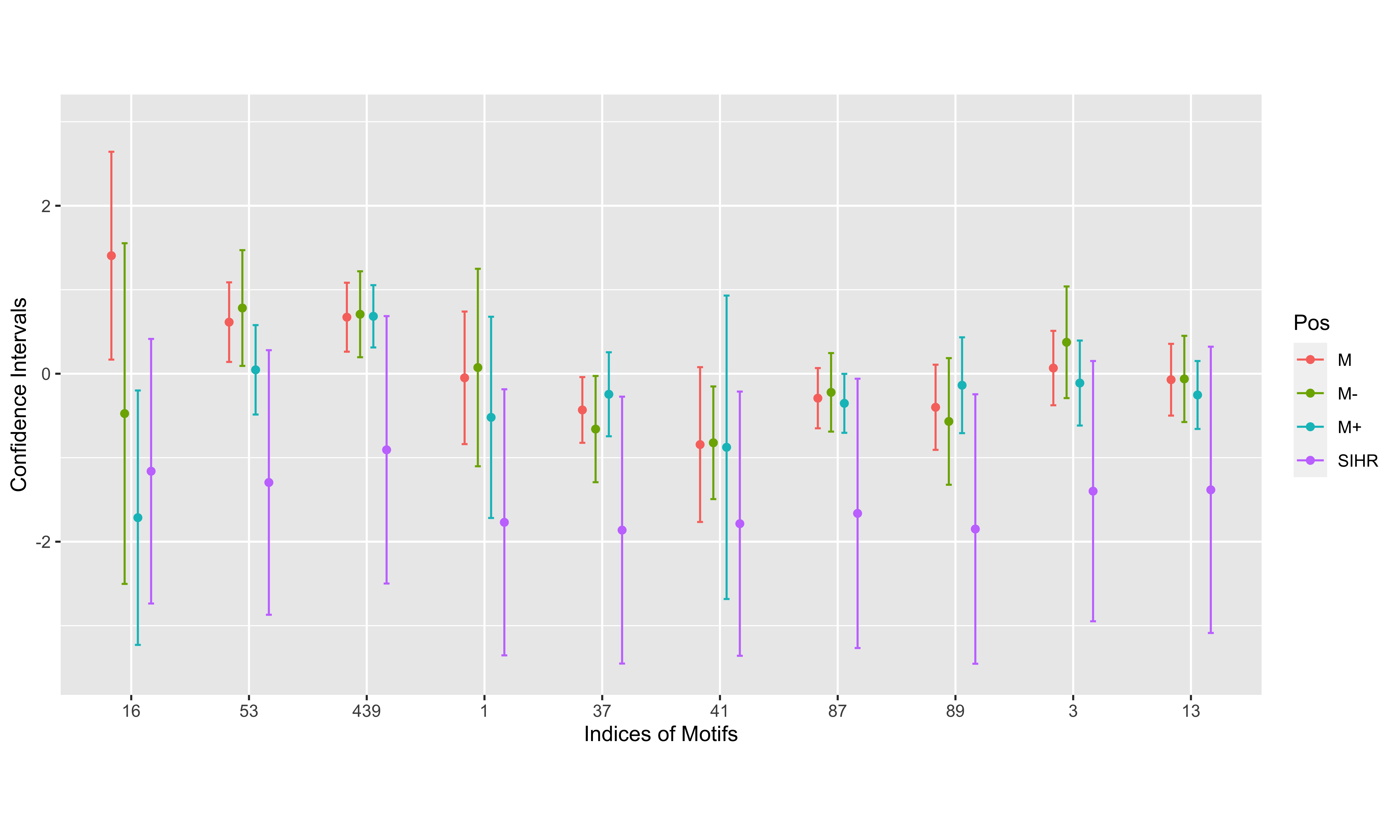
Figure 1: Confidence intervals for $f^{\prime}(a_{0})$ by DLL and SIHR. “M”,“M+” and “M-” represent the DLL estimator for $f^{\prime}(a_{0})$ with $a_{0}$ set as mean, mean + standard error and mean - standard error, respectively. SIHR represents inference for the constant effect in the high-dimensional linear model.

Figure 1 demonstrates several interesting observations. First of all, the CI lengths assuming the linear models are in general longer than those of DLL. This happens since the standard deviation of the regression error is about 2.5 by SIHR (assuming the linear model) but 1.45 by DLL (assuming the additive model). This indicates that the relationship between the gene expression levels and the motifs is highly non-linear. For constructing the local linear estimator, the DLL estimator only uses about 40% of the data while the SIHR estimator is computed with all data points.

Second, for the motifs with indexes 16, 53, and 439, we observe that those motifs do not have significant effects if we assume the effects to be linear. In contrast, our DLL estimator shows that they might have heterogeneous non-linear effects; for example, for motif 16, the CI at M- location is above zero while the CI at M+ is below zero. Lastly, the motifs with indexes 1, 37, 41, and 87 have significant linear effects, but their non-linear effects vary across different evaluation points.

We design a semi-real simulation study to further compare the finite-sample performance of our proposed DLL method and the SIHR method. We keep the data $\{D_{i},X_{i}\}_{1\leq i\leq 2587}$ the same as the real data. After analyzing the original real data, we construct the noise level estimator $\widehat{\sigma}^{2}$ and $\widehat{f}$ and $\widehat{g}$. We simulate the synthetic response variable $Y^{syn}_{i}=\widehat{f}(D_{i})+\widehat{g}(X_{i})+\bar{\epsilon}_{i}$ for $1\leq i\leq 2587$ with the i.i.d. regression error terms $\{\bar{\epsilon}_{i}\}_{1\leq i\leq 2587}$ following $N(0,\widehat{\sigma}^{2})$. We repeat the simulation 500 times and evaluate DLL on the same three evaluation points as in the real data analysis.

We compare the results with SIHR and report the comparison in Table 5. The SIHR method, which assumes the linear outcome model, suffers from a large absolute bias and low empirical coverage. Our proposed CIs by the DLL estimators achieve the desired coverage levels in most settings. The lengths of our proposed CIs are, in general, shorter or comparable to the CI output by SIHR. This happens since the regression noise level by SIHR is much larger than the true noise level due to the model misspecification. This matches with the observations for the original real data.

	Bias				SE				Coverage				Length
Motif	M	M+	M-	SIHR	M	M+	M-	SIHR	M	M+	M-	SIHR	M	M+	M-	SIHR
1	0.08	0.15	0.14	1.37	0.23	0.45	0.32	0.41	0.93	0.87	0.94	0.45	0.94	1.73	1.19	2.66
3	0.00	0.01	0.05	1.39	0.22	0.39	0.32	0.43	0.96	0.95	0.93	0.45	0.93	1.34	1.09	2.70
13	0.06	0.09	0.02	1.35	0.27	0.41	0.31	0.42	0.96	0.96	0.97	0.59	1.12	1.61	1.18	2.88
16	0.24	0.26	0.00	1.30	0.36	0.71	0.45	0.40	0.87	0.94	0.98	0.53	1.03	2.28	2.07	2.66
37	0.09	0.15	0.33	1.44	0.20	0.55	0.53	0.42	0.93	0.95	0.95	0.44	0.77	2.20	2.16	2.75
41	0.15	0.06	0.07	1.36	0.42	0.36	0.85	0.41	0.97	0.96	0.95	0.47	1.86	1.45	3.31	2.66
53	0.22	0.12	0.08	1.35	0.25	0.36	0.27	0.41	0.89	0.94	0.96	0.49	0.93	1.30	1.02	2.66
87	0.06	0.03	0.18	1.49	0.22	0.33	0.27	0.43	0.95	0.95	0.90	0.36	0.88	1.31	1.01	2.70
89	0.04	0.07	0.12	1.50	0.27	0.43	0.34	0.41	0.95	0.95	0.93	0.35	1.06	1.54	1.21	2.78
439	0.01	0.05	0.05	1.46	0.29	0.44	0.29	0.43	0.92	0.92	0.96	0.39	0.99	1.51	1.19	2.69

Table 5: Comparison of DLL and SIHR in the semi-real simulation study. The columns indexed with “M”,“M+” and “M-” report the performance of our proposed DLL inference methods for $f^{\prime}(a_{0})$, with $a_{0}$ set as mean, mean + standard error, and mean - standard error, respectively. SIHR refers to the high-dimensional inference methods assuming the linear model. The columns indexed with “Bias”, and “SE” report the absolute bias, and the standard error computed by 500 estimates, respectively; the columns indexed with “Coverage” report the empirical coverage level and the columns indexed with “Length” report the average CI length. For SIHR, the bias is taken as the minimal bias across the three evaluation points and the coverage is taken as the maximal coverage across the three evaluation points.

6 Conclusion and discussion

We have proposed the decorrelated local linear estimator to mitigate the error caused by estimating the unknown nuisance functions in the high-dimensional additive model. We have established the asymptotic normality of our proposed estimator. We demonstrate the validity of the theoretical results in moderate samples sizes and provide practical recommendations for the algorithm implementation. Our proposed decorrelation idea is a novel and computationally efficient method designed for bias correction in non-parametric models. An interesting future research direction is extending our proposed method to accommodate other kernel functions and higher-order local polynomials. In addition to inference for $f^{\prime}(a_{0}),$ there are other interesting statistical inference problems in the high-dimensional additive model, including confidence interval construction for $f(a_{0})$ and the significance test $H_{0}:f=0$. We leave these problems for future research.

Appendix A Additional Discussions

A.1 Algorithm without Data Swapping

In this section, we present the DLL estimator without data swapping. Different from the DLL estimator with data swapping, we use all the samples, rather than half of them, when fitting the sparse additive model and constructing the decorrelation weights. Following the steps of Algorithm 1, we make a few changes to implement the DLL estimator without data swapping.

In Step 1, implement the sparse additive model as the following optimization problem with $M\geq 1$ and $\lambda>0$:

$$\{\widehat{\beta}_{j}\}_{1\leq j\leq p}=\operatorname*{arg\,min}_{\beta_{j}\in\mathbb{R}^{M},\;0\leq j\leq p}\frac{1}{2n}\sum_{i=1}^{n}(Y_{i}-\sum_{j=0}^{p}\Psi_{i,j}^{\intercal}\beta_{j})^{2}+\lambda\sum_{j=0}^{p}\sqrt{\beta_{j}^{\intercal}\left(\frac{1}{n}\sum_{i=1}^{n}\Psi_{i,j}\Psi_{i,j}^{\intercal}\right)\beta_{j}}.$$ (31)

In Step 2, construct the initial estimator $\{\widehat{g}(X_{i})\}_{1\leq i\leq n}$ as:

$$\widehat{g}(X_{i})=\sum_{j=1}^{p}\Psi_{i,j}^{\intercal}\widehat{\beta}_{j}\quad\text{and}\quad\widehat{f}(D_{i})=\Psi_{i,0}^{\intercal}\widehat{\beta}_{0}.$$ (32)

In Step 5, implement Lasso algorithm as follows with the tuning parameter $\lambda_{1}>0$:

$$\widehat{\gamma}=\operatorname*{arg\,min}_{\gamma\in\mathbb{R}^{p}}\frac{1}{2n}\sum_{i=1}^{n}\left(D_{i}-X_{i}^{\intercal}\gamma\right)^{2}+\lambda_{1}\sum_{j=1}^{p}\frac{\|X_{j}\|_{2}}{\sqrt{n}}|\gamma_{j}|,$$

and compute

$$\widehat{\mu}_{i}=a_{0}-X_{i}^{\intercal}\widehat{\gamma}\quad\text{and}\quad\widehat{\delta}_{i}=D_{i}-X_{i}^{\intercal}\widehat{\gamma}\quad\text{for}\quad 1\leq i\leq n.$$

In Step 6, construct $\{\widehat{l}(X_{i})\}_{1\leq i\leq n}$ and the weights $\{\widetilde{W}_{i}\}_{1\leq i\leq n}$ as:

$$\widetilde{W}_{i}=(D_{i}-a_{0})-\widehat{l}(X_{i})\quad\text{with}\quad\widehat{l}(X_{i},\widehat{\gamma})=\frac{\frac{1}{n}\sum_{j=1}^{n}(\widehat{\delta}_{j}-\widehat{\mu}_{i}){\bf{1}}(|\widehat{\delta}_{j}-\widehat{\mu}_{i}|\leq h)}{\frac{1}{n}\sum_{j=1}^{n}{\bf{1}}(|\widehat{\delta}_{j}-\widehat{\mu}_{i}|\leq h)}.$$

The other steps are the same as Algorithm 1. We utilize the same parameter tuning procedures stated in Section 4. We compare our constructed confidence intervals with and without data swapping in Section F.3.

A.2 Double Penalization

In the following, we review the double penalization method [52] to construct initial estimators of $f$ and $g$. This can be viewed as an alternative method to the estimators in (31) and (32). To construct the penalty term, we define the complexity measure of a univariate function $f$ as

$$\mathcal{C}(f)=\lambda_{n}(\|f\|_{n}+\rho_{n}\|f\|_{F})$$ (33)

where $\lambda_{n}>0$, $\rho_{n}>0$, $\|f\|_{n}=(\sum_{i=1}^{n}f^{2}(D_{i}))^{1/2}$ denotes the function’s empirical $L_{2}$ norm, and $\|f\|_{F}=(\int[f^{\prime\prime}(t)]^{2}dt)^{1/2}$ is a measure of the function’s smoothness.

Specifically, with the positive tuning parameters $\rho_{n}>0$ and $\lambda_{n}>0$, we define the initial estimators as

$$\left\{\widehat{f},\left\{\widehat{g}_{j}\right\}_{1\leq j\leq p}\right\}=\arg\min\frac{1}{n}\sum_{i=1}^{n}[Y_{i}-f(D_{i})-\sum_{j=1}^{p}g_{j}(X_{ij})]^{2}+\mathcal{C}(f)+\sum_{j=1}^{p}\mathcal{C}(g_{j}),$$

where the complexity measure $\mathcal{C}(\cdot)$ is defined in (33).

A.3 Initial Estimators with Quantile Transformation

We consider the construction of the initial estimator $\widehat{g}$ by applying the quantile transformation to all variables. Particularly, we transform $D_{i}$ to $\widetilde{D}_{i}$, with

$$\widetilde{D}_{i}=\frac{\text{Ordering of }D_{i}}{n}\in(0,1];$$

similarly, for $1\leq j\leq p,$ we transform $X_{i,j}$ to $\widetilde{X}_{i,j}$, with

$$\widetilde{X}_{i,j}=\frac{\text{Ordering of }X_{i,j}}{n}\in(0,1].$$

We construct the initial estimators $\widehat{f}$ and $\widehat{g}$ by applying the sparse additive algorithm to $\{Y_{i},\widetilde{D}_{i},\widetilde{X}_{i}\}_{1\leq i\leq n}$. Except for constructing the initial estimator differently, the other steps are the same as those in Algorithm 1. This DLL estimator with the extra quantile transformation is refered to as Trans and we do not apply the data swapping for Trans estimator. We compare the performance of Trans with the regular DLL estimator in Section F.3; see Tables S10 and S11 for details.

A.4 Further discussions on the Condition (A3)

In a more general setting, we may plug-in the existing convergence rate of ${\rm Err}(\widehat{g})$ and then the condition (27) is reduced to a simultaneous condition on $k\coloneqq\|\gamma\|_{0}$ and $s\coloneqq\|g\|_{0}$, where $\|g\|_{0}$ denotes the number of non-zero functions of $\{g_{j}\}_{1\leq j\leq p}.$ Particularly, we follow [52] by assuming that the individual functions $\{g_{j}\}_{1\leq j\leq p}$ belong to the Sobolev space $\mathcal{W}^{m}_{2}$ for $m>1/2$ and $f^{\prime\prime}$ is continuous. We apply Proposition 4 and Theorem 2 in [52] and Corollaries 4 and 5 in [28] and establish that

$${\rm Err}^{2}(\widehat{g})\lesssim n^{-\frac{4}{5}}+s\cdot n^{-\frac{2m}{2m+1}}+(s+1)\cdot{\log p}/{n}.$$

Then the condition (27) is simplified as

$$k\cdot s\ll n^{\frac{2m}{2m+1}+\frac{3}{5}}\;\text{and}\;\max\{k,s\cdot n^{\frac{1}{2m+1}}\}\ll n\quad\text{up to a polynomial order of}\;\log p.$$

If we set $m=2$, then the above sparsity condition is much weaker than the one in [27], which requires $s\ll n^{\frac{3}{10}}$ and $k\ll n^{\frac{4}{15}}$ up to a polynomial order of $\log p.$

A.5 Consistent estimators of $\sigma^{2}$

Similar to the definition of ${\rm Err}(\widehat{g})$ in (26), we use ${\rm Err}(\widehat{f})$ to denote the accuracy measure of $\widehat{f}$, which is defined as follows: with probability larger than $1-\min$ for some positive constant $c>0,$

$$\sqrt{\mathbf{E}_{D_{*}}(\widehat{f}^{a}(D_{*})-f(D_{*}))^{2}+\mathbf{E}_{D_{*}}(\widehat{f}^{b}(D_{*})-f(D_{*}))^{2}}\lesssim{\rm Err}(\widehat{f}),$$ (34)

where $\widehat{f}^{a}$ and $\widehat{f}^{b}$ are defined in (22) and the expectation is taken with respect to the independent copy $D_{*}$ of $\{D_{i}\}_{1\leq i\leq n}.$

Proposition 1

Suppose that Condition (A1) holds and $\max\{{\rm Err}(\widehat{f}),{\rm Err}(\widehat{g})\}\rightarrow 0.$ Then the estimator $\widehat{\sigma}^{2}$ defined in (23) satisfies $\widehat{\sigma}^{2}\overset{p}{\to}\sigma^{2}.$

Proposition 1 shows that our proposed $\widehat{\sigma}^{2}$ is consistent if both $\widehat{f}$ and $\widehat{g}$ are consistent. The proof of Proposition 1 is presented in Section E.5.

Appendix B Notations, Events and Lemmas

We introduce some notations and events, which will be used throughout the proof. Let ${q}(D_{i}\mid X_{i})$ denote the conditional distribution of $D_{i}$ given $X_{i}$ and $\phi$ denote the density function of the error $\delta_{i}=D_{i}-X_{i}^{\intercal}\gamma.$ Since $D_{i}-X_{i}^{\intercal}\gamma$ is independent of $X_{i}$, we have

$${q}(D_{i}=a_{0}\mid X_{i})=\phi(a_{0}-X_{i}^{\intercal}{\gamma})=\phi(\mu_{i})\quad\text{with}\quad\mu_{i}=a_{0}-X_{i}^{\intercal}{\gamma}.$$

We express the density function $\pi$ of the random variable $D_{i}$ as

$$\pi(a_{0})=\mathbf{E}_{X_{i}}\left[{q}(D_{i}=a_{0}\mid X_{i})\right]=\mathbf{E}_{X_{i}}\left[\phi\left({a_{0}-X_{i}^{\intercal}{\gamma}}\right)\right].$$

Define the following events,

$$\mathcal{A}_{0} =\left\{\max_{i\in\mathcal{I}_{a}}\max_{\left|\delta-\mu_{i}\right|\leq r}\frac{|\phi^{\prime}(\delta)|}{\phi(\mu_{i})}\leq C_{1}(n),\quad\max_{i\in\mathcal{I}_{a}}\max_{\left|\delta-\mu_{i}\right|\leq r}\frac{|\phi^{\prime\prime}(\delta)|}{\phi(\mu_{i})}\leq C_{2}(n)\right\},$$ (35)

$$\mathcal{A}_{1} =\left\{\|\widehat{\gamma}^{b}-\gamma\|\lesssim\sqrt{\frac{k\log p}{n}},\;\max_{i\in\mathcal{I}_{a}}|X_{i}^{\intercal}(\widehat{\gamma}^{b}-\gamma)|\leq C^{*}\sqrt{\frac{k\log p\log n}{n}}\right\},$$

$$\mathcal{A}_{2} =\left\{\mathbf{E}_{X_{*}}(\widehat{g}^{b}(X_{*})-g(X_{*}))^{2}\lesssim{\rm Err}^{2}(\widehat{g})\right\}.$$

By the definitions of $C_{1}(n)$ and $C_{2}(n)$ in (24), we have $\mathbf{P}(\mathcal{A}_{0}^{c})\leq\min\{n,p\}^{-c}$ for some positive constant $c>0.$ Throughout the proof, we shall assume $\mathbf{P}(\mathcal{A}_{0}^{c})\ll h\pi(a_{0})$ and this will automatically hold in our considered regime.

Define $\mathcal{A}=\mathcal{A}_{0}\cap\mathcal{A}_{1}\cap\mathcal{A}_{2}$. Theorem 7.2 in [7] implies that the Lasso estimator $\widehat{\gamma}^{b}$ satisfies

$$\mathbf{P}\left(\|\widehat{\gamma}^{b}-\gamma\|\lesssim\sqrt{\frac{k\log p}{n}}\right)\geq 1-p^{-c},$$

for some positive constant $c>0$. Conditioning on the data in $\mathcal{I}_{b}$, the random variable ${X_{i}^{\intercal}(\widehat{\gamma}^{b}-\gamma)}/{\|\widehat{\gamma}^{b}-\gamma\|_{2}}$ is sub-gaussian random variable, which implies

$$\mathbf{P}\left(\max_{i\in\mathcal{I}_{a}}\left|{X_{i}^{\intercal}(\widehat{\gamma}^{b}-\gamma)}/{\|\widehat{\gamma}^{b}-\gamma\|_{2}}-\mathbf{E}\left[X_{i}^{\intercal}(\widehat{\gamma}^{b}-\gamma)/{\|\widehat{\gamma}^{b}-\gamma\|_{2}}\right|\mid\mathcal{I}_{b}\right]\gtrsim\sqrt{\log n}\mid\mathcal{I}_{b}\right)\leq n^{-c},$$

for some positive constant $c>0.$ Note that

$$\left|\mathbf{E}\left[X_{i}^{\intercal}(\widehat{\gamma}^{b}-\gamma)/{\|\widehat{\gamma}^{b}-\gamma\|_{2}}\mid\mathcal{I}_{b}\right]\right|\leq\sqrt{(\widehat{\gamma}-\gamma)^{\intercal}\Sigma(\widehat{\gamma}-\gamma)}/{\|\widehat{\gamma}^{b}-\gamma\|_{2}}\leq C.$$

The above two inequalities imply that, there exists a constant $C^{*}>0$ independent of $n$ and $p$ such that

$$\mathbf{P}\left(\max_{i\in\mathcal{I}_{a}}|X_{i}^{\intercal}(\widehat{\gamma}^{b}-\gamma)|\leq C^{*}\sqrt{\frac{k\log p\log n}{n}}\right)\geq 1-\min\{n,p\}^{-c},$$

for some positive constant $c>0.$ Together with the definition in (24) and (26), we establish

$$\mathbf{P}\left(\mathcal{A}\right)\geq 1-\min\{n,p\}^{c}\;\;\text{for some constant}\;c>1.$$ (36)

The following lemma states the expectation of terms involved with $K_{h}(D_{i})$, whose proof can be found in Section E.2.

Lemma 1

Suppose that Condition (A2) holds, then we have

$$\left|\frac{\mathbf{E}\left(K_{h}(D_{i})\mid X_{i}\right)}{{q}(a_{0}\mid X_{i})}-1\right|\cdot{{\bf 1}}_{\mathcal{A}_{0}}\leq\frac{h^{2}}{6}C_{2}(n);$$ (37)

$$\left|\frac{\mathbf{E}\left(K_{h}(D_{i})\right)}{\pi(a_{0})}-1\right|\lesssim{h^{2}}C_{2}(n)+\frac{\mathbf{P}(\mathcal{A}_{0}^{c})}{\pi(a_{0})};$$ (38)

$$\left|\frac{\mathbf{E}\left[(D_{i}-a_{0})K_{h}(D_{i})\right]}{{\pi}(a_{0})}\right|\leq\frac{1}{3}h^{2}(C_{1}(n)+\frac{3}{8}hC_{2}(n))+\frac{\mathbf{P}(\mathcal{A}_{0}^{c})}{{\pi}(a_{0})};$$ (39)

$$\left|\frac{\mathbf{E}\left[(D_{i}-a_{0})^{2}K_{h}(D_{i})\right]}{\frac{1}{3}h^{2}\pi(a_{0})}-1\right|\lesssim\frac{1}{10}h^{2}C_{2}(n)+\frac{\mathbf{P}(\mathcal{A}_{0}^{c})}{h\pi(a_{0})};$$ (40)

$$\left|\frac{\mathbf{E}\left({W}^{2}_{i}K_{h}(D_{i})\mid X_{i}\right)}{{\frac{1}{3}h^{2}q(a_{0}\mid X_{i})}}-1\right|\cdot\mathbf{1}_{\mathcal{A}_{0}}\lesssim h^{2}[C_{1}^{2}(n)+C_{2}(n)];$$ (41)

$$\left|\frac{\mathbf{E}W_{i}^{2}K_{h}^{2}(D_{i})}{\frac{1}{3}h\pi(a_{0})}-1\right|\lesssim h^{2}[C_{1}^{2}(n)+C_{2}(n)]+\frac{\mathbf{P}(\mathcal{A}_{0}^{c})}{h\pi(a_{0})};$$ (42)

$$\left|\frac{\mathbf{E}W_{i}(D_{i}-a_{0})K_{h}(D_{i})}{\frac{1}{3}h^{2}\pi(a_{0})}-1\right|\lesssim h^{2}[C_{1}^{2}(n)+C_{2}(n)]+\frac{\mathbf{P}(\mathcal{A}_{0}^{c})}{h\pi(a_{0})};$$ (43)

$$\left|\mathbf{E}W_{i}\frac{(D_{i}-a_{0})^{2}}{2}K_{h}(D_{i})\cdot\mathbf{1}_{\mathcal{A}_{0}^{c}}\right|\lesssim{h^{4}}\left[C_{1}(n)+hC_{2}(n)\right]\pi(a_{0})+h^{2}\mathbf{P}(\mathcal{A}_{0}^{c}).$$ (44)

The following lemma is about the concentration results for terms involved with $K_{h}(D_{i})$, whose proof can be found in Section E.3.

Lemma 2

Suppose that Condition (A2) holds, then for a sufficiently large $n$, with probability $1-\exp(-t^{2})$,

$$c\pi(a_{0})\left[1-\frac{t}{\sqrt{nh\pi(a_{0})}}\right]\leq\left|\frac{1}{n}\sum_{i=1}^{n}K_{h}(D_{i})\right|\leq C\pi(a_{0})\left[1+\frac{t}{\sqrt{nh\pi(a_{0})}}\right];$$ (45)

$$\left|\frac{1}{n}\sum_{i=1}^{n}W_{i}K_{h}(D_{i})\right|\lesssim t\sqrt{\frac{h}{n}\pi(a_{0})};$$ (46)

$$\left|\frac{1}{n}\sum_{i=1}^{n}{(D_{i}-a_{0})}K_{h}(D_{i})\right|\lesssim\frac{{\pi}(a_{0})}{3}h^{2}(C_{1}(n)+\frac{3}{8}hC_{2}(n))+{\mathbf{P}(\mathcal{A}_{0}^{c})}+t\sqrt{\frac{h}{n}\pi(a_{0})};$$ (47)

$$\left|\frac{1}{n}\sum_{i=1}^{n}W_{i}{(D_{i}-a_{0})}K_{h}(D_{i})-\mathbf{E}W_{i}(D_{i}-a_{0})K_{h}(D_{i})\right|\leq Ch^{2}\pi(a_{0})t\sqrt{\frac{1}{nh\pi(a_{0})}};$$ (48)

$$\left|\frac{1}{n}\sum_{i=1}^{n}W_{i}\frac{(D_{i}-a_{0})^{2}}{2}K_{h}(D_{i})\right|\lesssim{h^{4}}\left[C_{1}(n)+hC_{2}(n)\right]\pi(a_{0})+h^{2}\mathbf{P}(\mathcal{A}_{0}^{c})+t\sqrt{\frac{h^{5}}{n}\pi(a_{0})};$$ (49)

$$\left|\frac{1}{n}\sum_{i=1}^{n}W_{i}^{2}K_{h}^{2}(D_{i})-\mathbf{E}W_{i}^{2}K_{h}^{2}(D_{i})\right|\lesssim t\sqrt{\frac{h\pi(a_{0})}{{n}}}.$$ (50)

Combining (45) and (46), we establish that, with probability $1-\exp(-t^{2})$,

$$\left|\bar{\mu}_{W}\right|\lesssim t\sqrt{\frac{h}{n\pi(a_{0})}}.$$ (51)

Appendix C Proof of Theorem 2

Recall the definition of $\widehat{W}_{i}$ in (15). We define an accuracy measure of estimating the decorrelation weights as

$${\rm Err}(\widehat{W})=\sqrt{\frac{1}{n}\sum_{i=1}^{n}[\widehat{W}_{i}-\left({W}_{i}-\bar{\mu}_{W}\right)]^{2}K_{h}(D_{i})}\quad\text{with}\;\bar{\mu}_{W}=\frac{\frac{1}{n}\sum_{i=1}^{n}{W}_{i}K_{h}(D_{i})}{\frac{1}{n}\sum_{i=1}^{n}K_{h}(D_{i})}.$$ (52)

We first introduce the following important intermediate results. With probability larger than $1-\frac{C}{t^{2}}-\min\{n,p\}^{-c}$ for some $t>1$ and positive constants $C>0,c>0$,

$$\left|\frac{1}{n}\sum_{i=1}^{n}{W}_{i}\Delta(X_{i})K_{h}(D_{i})\right|\leq Ct\sqrt{{h}/{n}}\cdot{\rm Err}(\widehat{g}),$$ (53)

$$\left|{\frac{1}{n\widehat{S}_{n}}\sum_{i=1}^{n}\widehat{W}_{i}\Delta(X_{i})K_{h}(D_{i})}\right|\leq t\left(t\sqrt{\frac{1}{nh^{3}\pi^{2}(a_{0})}}+\frac{{\rm Err}(\widehat{W})}{h^{2}\pi(a_{0})}\right){\rm Err}(\widehat{g}),$$ (54)

and

$${\rm Err}(\widehat{W})\lesssim t\left(\sqrt{\frac{h}{n}}+\sqrt{\frac{k\log p\log n}{n}}h^{2}\left(C_{1}^{2}(n)+C_{2}(n)\right)\right).$$ (55)

A combination of (54) and (55) leads to the bound (29). We shall prove (53), (54), and (55) in Sections C.1, C.2, and C.3, respectively.

C.1 Proof of (53)

Recall the following notations,

• $\mathcal{I}_{a}$ and $\mathcal{I}_{b}$ are two disjoint subsets with approximately equal sample size, with $\mathcal{I}_{a}\cap\mathcal{I}_{b}$ empty and $\mathcal{I}_{a}\cup\mathcal{I}_{b}=\{1,2,\cdots,n\}.$

• $\widehat{g}^{a}$ and $\widehat{g}^{b}$ denote the initial estimator of $g$ based on the data $(X_{i},D_{i},Y_{i})_{i\in\mathcal{I}_{a}}$ and $(X_{i},D_{i},Y_{i})_{i\in\mathcal{I}_{b}}$, respectively.

The proof relies on the independence created by data swapping. Define the estimation error as $\Delta^{a}(X_{i})=\widehat{g}^{a}(X_{i})-g(X_{i})$ and $\Delta^{b}(X_{i})=\widehat{g}^{b}(X_{i})-g(X_{i}).$ We write $\mathbf{E}(\cdot\mid{\mathcal{I}_{a}})$,${\rm Var}(\cdot\mid{\mathcal{I}_{a}})$ and $\mathbf{P}(\cdot\mid{\mathcal{I}_{a}})$ as the expectation, variance and probability conditioning on the sample $(X_{i},D_{i},Y_{i})_{i\in\mathcal{I}_{a}},$ respectively. Similarly, we define $\mathbf{E}(\cdot\mid{\mathcal{I}_{b}}),{\rm Var}(\cdot\mid{\mathcal{I}_{b}})$ and $\mathbf{P}(\cdot\mid{\mathcal{I}_{b}})$ conditioning on $(X_{i},D_{i},Y_{i})_{i\in\mathcal{I}_{b}}$. For $1\leq i\leq n$, we have the following decomposition

$$\frac{1}{n}\sum_{i=1}^{n}{W}_{i}\Delta(X_{i})K_{h}(D_{i})=\frac{1}{n}\sum_{i\in\mathcal{I}_{a}}{W}_{i}\Delta^{b}(X_{i})K_{h}(D_{i})+\frac{1}{n}\sum_{i\in\mathcal{I}_{b}}{W}_{i}\Delta^{a}(X_{i})K_{h}(D_{i}).$$ (56)

We will control the first term $\frac{1}{n}\sum_{i\in\mathcal{I}_{a}}{W}_{i}\Delta^{b}(X_{i})K_{h}(D_{i})$ in the following and the second term can be controlled by a similar argument. Since

$$\mathbf{P}\left(|\frac{1}{n}\sum_{i\in\mathcal{I}_{a}}{W}_{i}\Delta^{b}(X_{i})K_{h}(D_{i})|\neq|\frac{1}{n}\sum_{i\in\mathcal{I}_{a}}{W}_{i}\Delta^{b}(X_{i})K_{h}(D_{i})\cdot\mathbf{1}_{\mathcal{A}_{0}\cap\mathcal{A}_{2}}|\right)\leq\min\{n,p\}^{-c},$$

it is sufficient to analyze

$$\frac{1}{n}\sum_{i=1}^{n}{W}_{i}\Delta^{b}(X_{i})K_{h}(D_{i})\cdot\mathbf{1}_{\mathcal{A}_{0}\cap\mathcal{A}_{2}},$$

where $\mathcal{A}_{0}$ and $\mathcal{A}_{2}$ are defined in (35). The above term has two sources of randomness: the initial estimator $\Delta^{b}=\widehat{g}^{b}-g$ and the data $\{X_{i},D_{i}\}_{i\in\mathcal{I}_{a}}$. Since the randomness of $\Delta^{b}$ is induced from the data $(X_{i},D_{i},Y_{i})_{i\in\mathcal{I}_{b}}$, the estimation error $\Delta^{b}$ is independent of the data $\{X_{i},D_{i}\}_{i\in\mathcal{I}_{a}}$.

Since ${W}_{i}$ is constructed such that $\mathbf{E}\left[{W}_{i}K_{h}(D_{i})\mid X_{i}\right]=0$, then we have

$$\mathbf{E}\left(\frac{1}{n}\sum_{i\in\mathcal{I}_{a}}{W}_{i}\Delta^{b}(X_{i})K_{h}(D_{i})\cdot\mathbf{1}_{\mathcal{A}_{0}\cap\mathcal{A}_{2}}\mid{\mathcal{I}_{b}},\{X_{i}\}_{i\in\mathcal{I}_{a}}\right)=0.$$ (57)

We control the second order moment as

$${\mathbf{E}}\left(\left(\frac{1}{n}\sum_{i\in\mathcal{I}_{a}}{W}_{i}\Delta^{b}(X_{i})K_{h}(D_{i})\cdot\mathbf{1}_{\mathcal{A}_{0}\cap\mathcal{A}_{2}}\right)^{2}\right)$$

$$=\mathbf{E}\left[{\mathbf{E}}\left(\left(\frac{1}{n}\sum_{i\in\mathcal{I}_{a}}{W}_{i}\Delta^{b}(X_{i})K_{h}(D_{i})\cdot\mathbf{1}_{\mathcal{A}_{0}\cap\mathcal{A}_{2}}\right)^{2}\mid{\mathcal{I}_{b}},\{X_{i}\}_{i\in\mathcal{I}_{a}}\right)\right]$$

$$=\frac{1}{n^{2}}\sum_{i\in\mathcal{I}_{a}}\mathbf{E}\left[\mathbf{E}\left(W^{2}_{i}K_{h}^{2}(D_{i})\mid{\mathcal{I}_{b}},\{X_{i}\}_{i\in\mathcal{I}_{a}}\right)(\Delta^{b}(X_{i}))^{2}\cdot\mathbf{1}_{\mathcal{A}_{0}\cap\mathcal{A}_{2}}\right],$$

where the last equality follows from (57). By (41) and the definition of ${\rm Err}(\widehat{g})$ in (26), we establish

$$\mathbf{E}\left[\mathbf{E}\left(W^{2}_{i}K_{h}^{2}(D_{i})\mid{\mathcal{I}_{b}},\{X_{i}\}_{i\in\mathcal{I}_{a}}\right)(\Delta^{b}(X_{i}))^{2}\cdot\mathbf{1}_{\mathcal{A}_{0}\cap\mathcal{A}_{2}}\right]\lesssim h{\rm Err}(\widehat{g})^{2}.$$

Hence we establish

$$\mathbf{P}\left(\left|\frac{1}{n}\sum_{i\in\mathcal{I}_{a}}{W}_{i}\Delta^{b}(X_{i})K_{h}(D_{i})\cdot\mathbf{1}_{\mathcal{A}_{0}\cap\mathcal{A}_{2}}\right|\leq t\sqrt{\frac{h}{n}}\cdot{\rm Err}(\widehat{g})\right)\geq 1-\frac{1}{t^{2}}-\min\{n,p\}^{-c}.$$

By symmetry and the decomposition (56), we establish (53).

C.2 Proof of (54)

We decompose $\frac{1}{n}\sum_{i=1}^{n}\widehat{W}_{i}\Delta(X_{i})K_{h}(D_{i})$ as

$$\frac{1}{n}\sum_{i=1}^{n}\left(\widehat{W}_{i}-\left({W}_{i}-\bar{\mu}_{W}\right)\right)\Delta(X_{i})K_{h}(D_{i})+\frac{1}{n}\sum_{i=1}^{n}{W}_{i}\Delta(X_{i})K_{h}(D_{i})-\bar{\mu}_{W}\cdot\frac{1}{n}\sum_{i=1}^{n}\Delta(X_{i})K_{h}(D_{i}).$$ (58)

By the Cauchy-Schwarz inequality, we have

$$\left|\frac{1}{n}\sum_{i=1}^{n}\left(\widehat{W}_{i}-\left({W}_{i}-\bar{\mu}_{W}\right)\right)\Delta(X_{i})K_{h}(D_{i})\right|\leq{\rm Err}(\widehat{W})\cdot\sqrt{\frac{1}{n}\sum_{i=1}^{n}\Delta(X_{i})^{2}K_{h}(D_{i})},$$ (59)

where ${\rm Err}(\widehat{W})$ is defined in (52). Hence, it is sufficient to control $\sqrt{\frac{1}{n}\sum_{i=1}^{n}\Delta(X_{i})^{2}K_{h}(D_{i})}.$ Similar to (56), we have

$$\frac{1}{n}\sum_{i=1}^{n}\Delta(X_{i})^{2}K_{h}(D_{i})=\frac{1}{n}\sum_{i\in\mathcal{I}_{a}}\left|\Delta^{b}(X_{i})\right|^{2}K_{h}(D_{i})+\frac{1}{n}\sum_{i\in\mathcal{I}_{b}}\left|\Delta^{a}(X_{i})\right|^{2}K_{h}(D_{i}),$$ (60)

and it is sufficient to control

$$\frac{1}{n}\sum_{i\in\mathcal{I}_{a}}\left|\Delta^{b}(X_{i})\right|^{2}K_{h}(D_{i})\cdot\mathbf{1}_{\mathcal{A}_{0}\cap\mathcal{A}_{2}}.$$

Note that

$${\mathbf{E}}\left(\frac{1}{n}\sum_{i\in\mathcal{I}_{a}}\left|\Delta^{b}(X_{i})\right|^{2}K_{h}(D_{i})\cdot\mathbf{1}_{\mathcal{A}_{0}\cap\mathcal{A}_{2}}\mid{\mathcal{I}_{b}},\{X_{i}\}_{i\in\mathcal{I}_{a}}\right)$$

$$= \frac{1}{n}\sum_{i\in\mathcal{I}_{a}}\left|\Delta^{b}(X_{i})\right|^{2}\cdot\mathbf{E}\left[K_{h}(D_{i})\mid X_{i}\right]\cdot\mathbf{1}_{\mathcal{A}_{0}\cap\mathcal{A}_{2}}\lesssim{\rm Err}^{2}(\widehat{g}),$$

where the last inequality follows from (37) and the bounded conditional density ${q}(a_{0}\mid X_{i}).$ The above moment bound implies

$$\mathbf{P}\left(\left|\frac{1}{n}\sum_{i=1}^{n}\left|\Delta^{b}(X_{i})\right|^{2}K_{h}(D_{i})\right|\leq Ct^{2}{\rm Err}^{2}(\widehat{g})\right)\geq 1-\frac{1}{t^{2}}-\min\{n,p\}^{-c}.$$

By symmetry and the decomposition (60), we have

$$\mathbf{P}\left(\left|\frac{1}{n}\sum_{i=1}^{n}\Delta(X_{i})^{2}K_{h}(D_{i})\right|\leq Ct^{2}{\rm Err}^{2}(\widehat{g})\right)\geq 1-\frac{1}{t^{2}}-\min\{n,p\}^{-c}.$$ (61)

Combined with (59), we obtain

$$\mathbf{P}\left(\left|\frac{1}{n}\sum_{i=1}^{n}\left(\widehat{W}_{i}-\left({W}_{i}-\bar{\mu}_{W}\right)\right)\Delta(X_{i})K_{h}(D_{i})\right|\lesssim t^{2}{\rm Err}(\widehat{W})\cdot{\rm Err}(\widehat{g})\right)\geq 1-\frac{1}{t^{2}}-\min\{n,p\}^{-c}.$$ (62)

Note that

$$\frac{1}{n}\sum_{i=1}^{n}\left|\Delta(X_{i})\right|K_{h}(D_{i})\leq\sqrt{\frac{1}{n}\sum_{i=1}^{n}K_{h}(D_{i})}\cdot\sqrt{\frac{1}{n}\sum_{i=1}^{n}\Delta(X_{i})^{2}K_{h}(D_{i})}.$$

Together with (45), (51), and (61), we establish

$$\mathbf{P}\left(\left|\bar{\mu}_{W}\cdot\frac{1}{n}\sum_{i=1}^{n}\Delta(X_{i})K_{h}(D_{i})\right|\lesssim t{\rm Err}(\widehat{g})\sqrt{{h}/{n}}\right)\geq 1-\frac{1}{t^{2}}-\min\{n,p\}^{-c}.$$

Together with (53), (62) and the decomposition (58), we have

$$\mathbf{P}\left(\left|\frac{1}{n}\sum_{i=1}^{n}\widehat{W}_{i}\Delta(X_{i})K_{h}(D_{i})\right|\lesssim t\left(t\sqrt{{h}/{n}}+{\rm Err}(\widehat{W})\right){\rm Err}(\widehat{g})\right)\geq 1-\frac{1}{t^{2}}-\min\{n,p\}^{-c}.$$

Together with (97), we establish (54).

C.3 Proof of (55)

In the following, we first establish

$${\rm Err}^{2}(\widehat{W})\lesssim{\frac{1}{n}\sum_{i=1}^{n}\left(l(X_{i},\widehat{\gamma})-l(X_{i},{\gamma})\right)^{2}K_{h}(D_{i})}.$$ (63)

Recall that the uncentered weight $\widetilde{W}_{i}$ is defined in (14) and $\widehat{W}_{i}$ is the corresponding centered weight defined in (15). Note that

$$\left(\widehat{W}_{i}-\left({W}_{i}-\bar{\mu}_{W}\right)\right)^{2}\lesssim\left(\widetilde{W}_{i}-{W}_{i}\right)^{2}+\left(\frac{\frac{1}{n}\sum_{i=1}^{n}(\widetilde{W}_{i}-{W}_{i})K_{h}(D_{i})}{\frac{1}{n}\sum_{i=1}^{n}K_{h}(D_{i})}\right)^{2}.$$ (64)

By Cauchy-Schwarz inequality

$$\left(\frac{1}{n}\sum_{i=1}^{n}(\widetilde{W}_{i}-{W}_{i})K_{h}(D_{i})\right)^{2}\leq\left(\frac{1}{n}\sum_{i=1}^{n}(\widetilde{W}_{i}-{W}_{i})^{2}K_{h}(D_{i})\right)\cdot\left(\frac{1}{n}\sum_{i=1}^{n}K_{h}(D_{i})\right),$$

we have

$$\frac{1}{n}\sum_{i=1}^{n}\left(\frac{\frac{1}{n}\sum_{i=1}^{n}(\widetilde{W}_{i}-{W}_{i})K_{h}(D_{i})}{\frac{1}{n}\sum_{i=1}^{n}K_{h}(D_{i})}\right)^{2}K_{h}(D_{i})\leq\frac{1}{n}\sum_{i=1}^{n}(\widetilde{W}_{i}-{W}_{i})^{2}K_{h}(D_{i}).$$

By applying the above inequality and (64), we obtain

$$\sqrt{\frac{1}{n}\sum_{i=1}^{n}\left(\widehat{W}_{i}-\left({W}_{i}-\bar{\mu}_{W}\right)\right)^{2}K_{h}(D_{i})}\lesssim\sqrt{\frac{1}{n}\sum_{i=1}^{n}\left(\widetilde{W}_{i}-{W}_{i}\right)^{2}K_{h}(D_{i})}$$

$$+\sqrt{\frac{1}{n}\sum_{i=1}^{n}\left(\frac{\frac{1}{n}\sum_{i=1}^{n}(\widetilde{W}_{i}-{W}_{i})K_{h}(D_{i})}{\frac{1}{n}\sum_{i=1}^{n}K_{h}(D_{i})}\right)^{2}K_{h}(D_{i})}\lesssim\sqrt{\frac{1}{n}\sum_{i=1}^{n}\left(\widetilde{W}_{i}-{W}_{i}\right)^{2}K_{h}(D_{i})}.$$

By the definitions ${W}_{i}=(D_{i}-a_{0})-l(X_{i},\gamma)$ and $\widetilde{W}_{i}=(D_{i}-a_{0})-\widehat{l}(X_{i},\widehat{\gamma}),$ the above inequality implies (63).

Then the proof of (55) is reduced to establishing an upper bound for

$${\frac{2}{n}\sum_{i=1}^{n}\left(\widehat{l}(X_{i},\widehat{\gamma})-l(X_{i},{\gamma})\right)^{2}K_{h}(D_{i})}.$$

We divide the above summation into two parts,

$${\frac{1}{n_{a}}\sum_{i\in\mathcal{I}_{a}}\left(\widehat{l}(X_{i},\widehat{\gamma}^{b})-l(X_{i},{\gamma})\right)^{2}K_{h}(D_{i})}+{\frac{1}{n_{b}}\sum_{i\in\mathcal{I}_{b}}\left(\widehat{l}(X_{i},\widehat{\gamma}^{a})-l(X_{i},{\gamma})\right)^{2}K_{h}(D_{i})}.$$

By symmetry, we focus on the first summation

$${\frac{1}{n_{a}}\sum_{i\in\mathcal{I}_{a}}\left(\widehat{l}(X_{i},\widehat{\gamma}^{b})-l(X_{i},{\gamma})\right)^{2}K_{h}(D_{i})},$$ (65)

and adopt the notation $\widehat{\gamma}^{b}=\widehat{\gamma}.$ We note that

$$\widehat{\delta}_{j}-\widehat{\mu}_{i}=\delta_{j}-\mu_{i}-a_{ij},\quad\text{with}\quad a_{ij}=(X_{j}-X_{i})^{\intercal}(\widehat{\gamma}-\gamma).$$

On the event $\mathcal{A}_{1}$ defined in (35), we have

$$|a_{ij}|\leq C^{*}\sqrt{\frac{\|\gamma\|_{0}\log p}{n}}\sqrt{\log n}.$$ (66)

To facilitate the discussion, we introduce the following notations,

$$\widehat{{\bf I}}_{ij}={\bf{1}}(|\delta_{j}-\mu_{i}-a_{ij}|\leq h)\quad\text{and}\quad{\bf I}_{ij}={\bf{1}}(|\delta_{j}-\mu_{i}|\leq h).$$ (67)

The estimator $\widehat{l}(X_{i},\widehat{\gamma})$ defined in (13) can be written as

$$\widehat{l}(X_{i},\widehat{\gamma})=\frac{\frac{1}{n_{a}}\sum_{j\in\mathcal{I}_{a}}(\delta_{j}-\mu_{i}-a_{ij})\widehat{{\bf I}}_{ij}}{\frac{1}{n_{a}}\sum_{j\in\mathcal{I}_{a}}\widehat{{\bf I}}_{ij}}.$$ (68)

The randomness of $\widehat{l}(X_{i},\widehat{\gamma})$ comes from the following three parts,

• the noise $\{\delta_{j}\}_{j\in\mathcal{I}_{a}}$

• the variable $\mu_{i}$ with $\mu_{i}=a_{0}-X^{\intercal}_{i}\gamma$ for the pre-fixed index $i$

• the estimation error $a_{ij}$, which depends on $X_{i},X_{j}$ and the initial estimator $\widehat{\gamma}$ computed on the data $\mathcal{I}_{b}$.

Note that $\{\delta_{j}\}_{j\in\mathcal{I}_{a}}$ is independent of the other two random sources. We shall write $\mathbf{E}_{\delta_{j}}$ as the expectation with respect to $\delta_{j}$ but condition on the other two components $X_{i}$ and $\mathcal{I}_{b}$. We use $\mathbf{E}_{\delta_{j}}\left[\cdot\mid\widehat{{\bf I}}_{ij}\right]$ to denote the conditional expectation by only considering the randomness of $\delta_{j}$. Specifically, for $j\in\mathcal{I}_{a}$, $\mathbf{E}_{\delta_{j}}$ and $\mathbf{E}_{\delta_{j}}\left[\cdot\mid\widehat{{\bf I}}_{ij}\right]$ are shorthanded for

$$\mathbf{E}_{\delta_{j}}[\cdot]=\mathbf{E}[\cdot\mid\{X_{i}\}_{i\in\mathcal{I}_{a}},\mathcal{I}_{b}]\quad\text{and}\quad\mathbf{E}_{\delta_{j}}\left[\cdot\mid\widehat{{\bf I}}_{ij}\right]=\mathbf{E}\left[\cdot\mid\widehat{{\bf I}}_{ij},\{X_{i}\}_{i\in\mathcal{I}_{a}},\mathcal{I}_{b}\right].$$

We use $\mathbf{E}_{\delta\mid\widehat{{\bf I}}_{i\cdot}}$ to denote the conditional expectation of $\{\delta_{j}\}_{j\in\mathcal{I}_{a}}$ given the events $\widehat{{\bf I}}_{i\cdot}=\{\widehat{{\bf I}}_{ij}\}_{j\in\mathcal{I}_{a}},$ by only considering the randomness of $\{\delta_{j}\}_{j\in\mathcal{I}_{a}},$ that is

$$\mathbf{E}_{\delta\mid\widehat{{\bf I}}_{i\cdot}}[\cdot]=\mathbf{E}\left[\cdot\mid\widehat{{\bf I}}_{i\cdot},\{X_{i}\}_{i\in\mathcal{I}_{a}},\mathcal{I}_{b}\right].$$

We compute the following difference,

$$\frac{\frac{1}{n_{a}}\sum_{j\in\mathcal{I}_{a}}(\delta_{j}-\mu_{i}-a_{ij})\widehat{{\bf I}}_{ij}}{\frac{1}{n_{a}}\sum_{j\in\mathcal{I}_{a}}\widehat{{\bf I}}_{ij}}-\frac{\frac{1}{n_{a}}\sum_{j\in\mathcal{I}_{a}}\mathbf{E}_{\delta_{j}}\left[(\delta_{j}-\mu_{i}-a_{ij})\widehat{{\bf I}}_{ij}\mid\widehat{{\bf I}}_{ij}\right]}{\frac{1}{n_{a}}\sum_{j\in\mathcal{I}_{a}}\widehat{{\bf I}}_{ij}}$$ (69)

$$=\frac{\frac{1}{n_{a}}\sum_{j\in\mathcal{I}_{a}}\widehat{{\bf I}}_{ij}\left((\delta_{j}-\mu_{i}-a_{ij})-\mathbf{E}_{\delta_{j}}\left(\delta_{j}-\mu_{i}-a_{ij}\mid\widehat{{\bf I}}_{ij}\right)\right)}{\frac{1}{n_{a}}\sum_{j\in\mathcal{I}_{a}}\widehat{{\bf I}}_{ij}}.$$

Define

$$F_{ij}(t)=\frac{\int_{\mu_{i}+ta_{ij}-h}^{\mu_{i}+ta_{ij}+h}(\delta-\mu_{i}-ta_{ij})\phi(\delta)d\delta}{\int_{\mu_{i}+ta_{ij}-h}^{\mu_{i}+ta_{ij}+h}\phi(\delta)d\delta}.$$ (70)

Note that

$$\mathbf{E}_{\delta_{j}}\left(\delta_{j}-\mu_{i}-a_{ij}\mid\widehat{{\bf I}}_{ij}\right)=\frac{\int_{\mu_{i}+a_{ij}-h}^{\mu_{i}+a_{ij}+h}(\delta-\mu_{i}-a_{ij})\phi(\delta)d\delta}{\int_{\mu_{i}+a_{ij}-h}^{\mu_{i}+a_{ij}+h}\phi(\delta)d\delta}=F_{ij}(1).$$ (71)

By (68), (69), and (71), we establish

$$\widehat{l}(X_{i},\widehat{\gamma})-{l}(X_{i},{\gamma})=\frac{\frac{1}{n_{a}}\sum_{j\in\mathcal{I}_{a}}(\delta_{j}-\mu_{i}-a_{ij})\widehat{{\bf I}}_{ij}}{\frac{1}{n_{a}}\sum_{j\in\mathcal{I}_{a}}\widehat{{\bf I}}_{ij}}-\frac{\int_{\mu_{i}-h}^{\mu_{i}+h}\left(\delta-\mu_{i}\right)\phi(\delta)d\delta}{\int_{\mu_{i}-h}^{\mu_{i}+h}\phi(\delta)d\delta}$$ (72)

$$=\frac{\frac{1}{n_{a}}\sum_{j\in\mathcal{I}_{a}}\widehat{{\bf I}}_{ij}\left[(\delta_{j}-\mu_{i}-a_{ij})-\mathbf{E}_{\delta_{j}}\left(\delta_{j}-\mu_{i}-a_{ij}\mid\widehat{{\bf I}}_{ij}\right)\right]}{\frac{1}{n_{a}}\sum_{j\in\mathcal{I}_{a}}\widehat{{\bf I}}_{ij}}+\frac{\frac{1}{n_{a}}\sum_{j\in\mathcal{I}_{a}}\widehat{{\bf I}}_{ij}\left[F_{ij}(1)-F_{ij}(0)\right]}{\frac{1}{n_{a}}\sum_{j\in\mathcal{I}_{a}}\widehat{{\bf I}}_{ij}},$$

where the last component holds since $F_{ij}(0)$ defined in (70) does not depend on the index $j$.

The decomposition (72) and the following two inequalities lead to an upper bound for (65).

$$\frac{1}{n_{a}}\sum_{i\in\mathcal{I}_{a}}\mathbf{E}\left[\left(\frac{\frac{1}{n_{a}}\sum_{j\in\mathcal{I}_{a}}\widehat{{\bf I}}_{ij}\left[(\delta_{j}-\mu_{i}-a_{ij})-\mathbf{E}_{\delta_{j}}\left(\delta_{j}-\mu_{i}-a_{ij}\mid\widehat{{\bf I}}_{ij}\right)\right]}{\frac{1}{n_{a}}\sum_{j\in\mathcal{I}_{a}}\widehat{{\bf I}}_{ij}}\right)^{2}\frac{1}{2h}{\bf{1}}(|\delta_{i}-\mu_{i}|\leq h)\right]\lesssim\frac{h}{n_{a}},$$ (73)

and

$$\frac{1}{n_{a}}\sum_{i\in\mathcal{I}_{a}}\mathbf{E}\left[\left(\frac{\frac{1}{n_{a}}\sum_{j\in\mathcal{I}_{a}}\widehat{{\bf I}}_{ij}\left[F_{ij}(1)-F_{ij}(0)\right]}{\frac{1}{n_{a}}\sum_{j\in\mathcal{I}_{a}}\widehat{{\bf I}}_{ij}}\right)^{2}\frac{1}{2h}{\bf{1}}(|\delta_{i}-\mu_{i}|\leq h)\cdot{{\bf 1}}_{\mathcal{A}_{0}\cap\mathcal{A}_{1}}\right]$$ (74)

$$\lesssim h^{4}\left(C_{1}^{2}(n)+C_{2}(n)\right)^{2}\frac{k\log p\log n}{n}.$$

We establish (55) by combining (63), (72), (73), (74), and (36).

C.3.1 Proof of (73)

In the following proof, we fix $i\in\mathcal{I}_{a}$ and ${{\bf I}}_{ii}=\widehat{{\bf I}}_{ii}.$ For $j_{1},j_{2}\in\mathcal{I}_{a}$ with $j_{1}\neq j_{2},$

$$\mathbf{E}_{\delta\mid\widehat{{\bf I}}_{i\cdot}}\left[(\delta_{j_{1}}-\mu_{i}-a_{i{j_{1}}})-\mathbf{E}_{\delta_{j_{1}}}\left(\delta_{j_{1}}-\mu_{i}-a_{i{j_{1}}}\mid\widehat{{\bf I}}_{i{j_{1}}}\right)\right]\left[(\delta_{j_{2}}-\mu_{i}-a_{i{j_{2}}})-\mathbf{E}_{\delta_{j_{2}}}\left(\delta_{j_{2}}-\mu_{i}-a_{i{j_{2}}}\mid\widehat{{\bf I}}_{i{j_{2}}}\right)\right]=0,$$

and

$$\mathbf{E}_{\delta_{j}\mid\widehat{{\bf I}}_{ij}}\left[(\delta_{j}-\mu_{i}-a_{ij})-\mathbf{E}_{\delta_{j}}\left(\delta_{j}-\mu_{i}-a_{ij}\mid\widehat{{\bf I}}_{ij}\right)\right]^{2}\leq\mathbf{E}_{\delta_{j}\mid\widehat{{\bf I}}_{ij}}\left[(\delta_{j}-\mu_{i}-a_{ij})\right]^{2}\leq h^{2}.$$

By the above two expressions, we obtain

$$\mathbf{E}_{\delta\mid\widehat{{\bf I}}_{i\cdot}}\left[\left(\frac{\frac{1}{n_{a}}\sum_{j\in\mathcal{I}_{a}}\widehat{{\bf I}}_{ij}\left[(\delta_{j}-\mu_{i}-a_{ij})-\mathbf{E}_{\delta_{j}}\left(\delta_{j}-\mu_{i}-a_{ij}\mid\widehat{{\bf I}}_{ij}\right)\right]}{\frac{1}{n_{a}}+\frac{1}{n_{a}}\sum_{j\neq i}\widehat{{\bf I}}_{ij}}\right)^{2}\frac{1}{2h}{{\bf I}}_{ii}\right]$$ (75)

$$=\frac{\frac{1}{n_{a}^{2}}\sum_{j\in\mathcal{I}_{a}}\widehat{{\bf I}}_{ij}\mathbf{E}_{\delta_{j}\mid\widehat{{\bf I}}_{ij}}\left[(\delta_{j}-\mu_{i}-a_{ij})-\mathbf{E}_{\delta_{j}}\left(\delta_{j}-\mu_{i}-a_{ij}\mid\widehat{{\bf I}}_{ij}\right)\right]^{2}}{\left(\frac{1}{n_{a}}+\frac{1}{n_{a}}\sum_{j\neq i}\widehat{{\bf I}}_{ij}\right)^{2}}\frac{1}{2h}{{\bf I}}_{ii}$$

$$\leq\frac{h}{2n_{a}}\frac{{{\bf I}}_{ii}}{\frac{1}{n_{a}}+\frac{1}{n_{a}}\sum_{j\neq i}\widehat{{\bf I}}_{ij}},$$

We further take expectation with respect to ${\bf I}$ (but conditioning on $\mu_{i}$ and $a_{ij}$) in (75) and obtain that

$$\mathbf{E}_{\delta}\left(\frac{h}{n_{a}}\frac{{{\bf I}}_{ii}}{\frac{1}{n_{a}}+\frac{1}{n_{a}}\sum_{j\neq i}\widehat{{\bf I}}_{ij}}\right)=\frac{h}{n_{a}}\cdot(\mathbf{E}_{\delta}{{\bf I}}_{ii})\cdot\left(\mathbf{E}_{\delta}\frac{1}{\frac{1}{n_{a}}+\frac{1}{n_{a}}\sum_{j\neq i}\widehat{{\bf I}}_{ij}}\right).$$ (76)

Conditioning on $\mu_{i}$ and $a_{ij},$ we define the conditional probability with respect to $\delta_{j}$ as

$$e_{ij}=\mathbf{E}_{\delta_{j}}[\widehat{{\bf I}}_{ij}]=\int_{\mu_{i}+a_{ij}-h}^{\mu_{i}+a_{ij}+h}\phi(\delta_{j})d\delta_{j}.$$ (77)

By change of variable $\tau_{j}=\delta_{j}-(\mu_{i}+a_{ij})$, we have

$$\int_{\mu_{i}+a_{ij}-h}^{\mu_{i}+a_{ij}+h}\phi(\delta_{j})d\delta_{j} =\int_{-h}^{h}\phi(\tau_{j}+\mu_{i}+a_{ij})d\tau_{j}$$

$$=\int_{-h}^{h}[\phi(\mu_{i}+a_{ij})+\tau_{j}\phi^{\prime}(\mu_{i}+a_{ij})+\frac{\tau_{j}^{2}}{2}\phi^{\prime\prime}(\mu_{i}+a_{ij}+c\tau_{j})]d\tau_{j},$$

for some constant $c\in(0,1).$ Hence, we have

$$\left|\int_{\mu_{i}+a_{ij}-h}^{\mu_{i}+a_{ij}+h}\phi(\delta_{j})d\delta_{j}-2h\phi(\mu_{i}+a_{ij})\right|\leq\frac{h^{3}}{3}\max_{|c|\leq 1}\left|\phi^{\prime\prime}(\mu_{i}+a_{ij}+ch)\right|,$$

and then

$$\left|e_{ij}-2h\phi(\mu_{i})\right|\leq\frac{h^{3}}{3}\max_{|c|\leq 1}\left|\phi^{\prime\prime}(\mu_{i}+a_{ij}+ch)\right|+2h|a_{ij}|\max_{|c|\leq 1}\left|\phi^{\prime}(\mu_{i}+ca_{ij})\right|.$$

Hence, we establish

$$\left|\frac{e_{ij}}{2h\phi(\mu_{i})}-1\right|\leq\frac{h^{2}}{3}C_{2}(n)+|a_{ij}|C_{1}(n).$$ (78)

We note that the non-negative random variable $\frac{1}{n_{a}}\sum_{j\neq i}\widehat{{\bf I}}_{ij}$ satisfies

$$\mathbf{E}\left[\frac{1}{n_{a}}\sum_{j\neq i}\widehat{{\bf I}}_{ij}\mid\{X_{i}\}_{i\in\mathcal{I}_{a}},\mathcal{I}_{b}\right]=\frac{1}{n_{a}}\sum_{j\neq i}e_{ij},$$

and

$${\rm Var}\left[\frac{1}{n_{a}}\sum_{j\neq i}\widehat{{\bf I}}_{ij}\mid\{X_{i}\}_{i\in\mathcal{I}_{a}},\mathcal{I}_{b}\right]=\frac{1}{n_{a}^{2}}\sum_{j\neq i}e_{ij}(1-e_{ij}).$$

Hence, we apply the equation (5) in [56] and obtain

$$\mathbf{E}_{\delta}\left[\frac{1}{\frac{1}{n_{a}}+\frac{1}{n_{a}}\sum_{j\neq i}\widehat{{\bf I}}_{ij}}\right] =\mathbf{E}\left[\frac{1}{\frac{1}{n_{a}}+\frac{1}{n_{a}}\sum_{j\neq i}\widehat{{\bf I}}_{ij}}\mid\{X_{i}\}_{i\in\mathcal{I}_{a}},\mathcal{I}_{b}\right]$$ (79)

$$\leq\frac{1}{\frac{1}{n_{a}}\sum_{j\neq i}e_{ij}+\frac{1}{n_{a}}}\left(1+\frac{\frac{1}{n_{a}^{2}}\sum_{j\neq i}e_{ij}(1-e_{ij})}{\frac{1}{n_{a}^{2}}\sum_{j\neq i}e_{ij}}\right)$$

$$\leq\frac{2}{\frac{1}{n_{a}}\sum_{j\neq i}e_{ij}+\frac{1}{n_{a}}}.$$

A combination of (76), (78) and (79) leads to

$$\mathbf{E}_{\delta}\left(\frac{h}{n_{a}}\frac{{{\bf I}}_{ii}}{\frac{1}{n_{a}}+\frac{1}{n_{a}}\sum_{j\neq i}\widehat{{\bf I}}_{ij}}\right)\leq\frac{h}{n_{a}}\frac{2e_{ii}}{\frac{1}{n_{a}}\sum_{j\neq i}e_{ij}+\frac{1}{n_{a}}}\lesssim\frac{h}{n_{a}}.$$ (80)

By taking expectation with respect to $\{X_{i}\}_{i\in\mathcal{I}_{a}}$ and $\mathcal{I}_{b},$ we establish (73).

C.3.2 Proof of (74)

We calculate the expression of $F_{ij}(t)$ in (70) as

$$\frac{dF_{ij}(t)}{dt} =\frac{a_{ij}h\left[\phi(\mu_{i}+ta_{ij}+h)+\phi(\mu_{i}+ta_{ij}-h)-\frac{1}{h}\int_{\mu_{i}+ta_{ij}-h}^{\mu_{i}+ta_{ij}+h}\phi(\delta_{j})d\delta_{j}\right]}{\int_{\mu_{i}+ta_{ij}-h}^{\mu_{i}+ta_{ij}+h}\phi(\delta_{j})d\delta_{j}}$$ (81)

$$-\frac{\int_{\mu_{i}+ta_{ij}-h}^{\mu_{i}+ta_{ij}+h}(\delta_{j}-\mu_{i}-ta_{ij})\phi(\delta_{j})d\delta_{j}}{\left[\int_{\mu_{i}+ta_{ij}-h}^{\mu_{i}+ta_{ij}+h}\phi(\delta_{j})d\delta_{j}\right]^{2}}\cdot a_{ij}\left[\phi(\mu_{i}+ta_{ij}+h)-\phi(\mu_{i}+ta_{ij}-h)\right].$$

Define

$$T_{1}(a_{ij})=\phi(\mu_{i}+ta_{ij}+h)+\phi(\mu_{i}+ta_{ij}-h)-\frac{1}{h}\int_{\mu_{i}+ta_{ij}-h}^{\mu_{i}+ta_{ij}+h}\phi(\delta_{j})d\delta_{j};$$

$$T_{2}(a_{ij})=\phi(\mu_{i}+ta_{ij}+h)-\phi(\mu_{i}+ta_{ij}-h);$$

and

$$T_{3}(a_{ij})=\int_{\mu_{i}+ta_{ij}-h}^{\mu_{i}+ta_{ij}+h}[\delta_{j}-(\mu_{i}+ta_{ij})]\phi(\delta_{j})d\delta_{j}.$$

Then we can simplify the derivative of $F_{ij}(t)$ in (81) as

$$\frac{dF_{ij}(t)}{dt}=\frac{ha_{ij}T_{1}(a_{ij})}{e_{ij}}-\frac{a_{ij}T_{2}(a_{ij})}{e_{ij}}\cdot\frac{T_{3}(a_{ij})}{e_{ij}},$$ (82)

where $e_{ij}$ is defined in (77). To bound the above terms, we introduce the following lemma to control all of the above terms.

Lemma 3

Suppose that $\phi(t)$ is twice differentiable for $t\in[\mu-\tau,\mu+\tau],$ there exists some positive constant $C>0$ such that

$$\left|\phi(\mu+\tau)+\phi(\mu-\tau)-\frac{1}{\tau}\int_{\mu-\tau}^{\mu+\tau}\phi(t)dt\right|\leq C\tau^{2}\cdot\max_{t\in[\mu-\tau,\mu+\tau]}\left|\phi^{\prime\prime}(t)\right|$$ (83)

$$\left|\int_{\mu-\tau}^{\mu+\tau}\left(t-\mu\right)\phi(t)dt\right|\leq C\tau^{3}\max_{t\in[\mu-\tau,\mu+\tau]}\left|\phi^{\prime}(t)\right|$$ (84)

$$\left|\phi(\mu+\tau)-\phi(\mu-\tau)\right|\leq C\tau\max_{t\in[\mu-\tau,\mu+\tau]}\left|\phi^{\prime}(t)\right|$$ (85)

It follows from (83) that

$$\left|T_{1}(a_{ij})\right|\lesssim h^{2}\cdot\max_{\left|\delta-(\mu_{i}+ta_{ij})\right|\leq h}|\phi^{\prime\prime}(\delta)|\leq h^{2}\cdot\max_{\left|\delta-\mu_{i}\right|\leq r}|\phi^{\prime\prime}(\delta)|.$$

It follows from (84) that

$$\left|T_{2}(a_{ij})\right|\lesssim h\cdot\max_{\left|\delta-(\mu_{i}+ta_{ij})\right|\leq h}|\phi^{\prime}(\delta)|\leq h\cdot\max_{\left|\delta-\mu_{i}\right|\leq r}|\phi^{\prime}(\delta)|.$$

It follows from (85) that

$$\left|T_{3}(a_{ij})\right|\lesssim h^{3}\cdot\max_{\left|\delta-(\mu_{i}+ta_{ij})\right|\leq h}|\phi^{\prime}(\delta)|\leq h^{3}\cdot\max_{\left|\delta-\mu_{i}\right|\leq r}|\phi^{\prime}(\delta)|.$$

Together with (78), we establish

$$\frac{\left|T_{1}(a_{ij})\right|}{e_{ij}}\lesssim h\cdot\max_{\left|\delta-\mu_{i}\right|\leq r}\frac{|\phi^{\prime\prime}(\delta)|}{\phi(\mu_{i})},\quad\frac{\left|T_{2}(a_{ij})\right|}{e_{ij}}\lesssim\max_{\left|\delta-\mu_{i}\right|\leq r}\frac{|\phi^{\prime}(\delta)|}{\phi(\mu_{i})},\quad\frac{\left|T_{3}(a_{ij})\right|}{e_{ij}}\lesssim h^{2}\cdot\max_{\left|\delta-\mu_{i}\right|\leq r}\frac{|\phi^{\prime}(\delta)|}{\phi(\mu_{i})},$$

where $r=C^{*}\sqrt{{\|\gamma\|_{0}\log p\log n}/{n}}+h.$ Together with the expression (82) and the upper bound (66), we establish

$$\left|\frac{dF_{ij}(t)}{dt}\right|{{\bf 1}}_{\mathcal{A}_{0}\cap\mathcal{A}_{1}}\lesssim\sqrt{\frac{k\log p\log n}{n}}h^{2}\left(C^{2}_{1}(n)+C_{2}(n)\right).$$

Hence, we have

$$\left(\frac{\frac{1}{n_{a}}\sum_{j\in\mathcal{I}_{a}}\widehat{{\bf I}}_{ij}\left[F_{ij}(1)-F_{ij}(0)\right]}{\frac{1}{n_{a}}\sum_{j\in\mathcal{I}_{a}}\widehat{{\bf I}}_{ij}}\right)^{2}{{\bf 1}}_{\mathcal{A}_{0}\cap\mathcal{A}_{1}}\lesssim\left(\sqrt{\frac{k\log p\log n}{n}}h^{2}\left(C_{1}^{2}(n)+C_{2}(n)\right)\right)^{2},$$

and

$$\frac{1}{n_{a}}\sum_{i=1}^{n_{a}}\mathbf{E}\left(\frac{\frac{1}{n_{a}}\sum_{j\in\mathcal{I}_{a}}\widehat{{\bf I}}_{ij}\left[F_{ij}(1)-F_{ij}(0)\right]}{\frac{1}{n_{a}}\sum_{j\in\mathcal{I}_{a}}\widehat{{\bf I}}_{ij}}\right)^{2}\frac{1}{2h}{\bf{1}}(|\delta_{i}-\mu_{i}|\leq h)\cdot{{\bf 1}}_{\mathcal{A}_{0}\cap\mathcal{A}_{1}}$$ (86)

$$\lesssim\left(\sqrt{\frac{k\log p\log n}{n}}h^{2}\left(C_{1}^{2}(n)+C_{2}(n)\right)\right)^{2}\frac{1}{n_{a}}\sum_{i=1}^{n_{a}}\mathbf{E}\frac{1}{2h}{\bf{1}}(|\delta_{i}-\mu_{i}|\leq h)$$

$$=\left(\sqrt{\frac{k\log p\log n}{n}}h^{2}\left(C_{1}^{2}(n)+C_{2}(n)\right)\right)^{2}\frac{1}{n_{a}}\sum_{i=1}^{n_{a}}\mathbf{E}K_{h}(D_{i}).$$

Together with (38), we establish (74).

Appendix D Proof of Theorem 1

We start with the following error decomposition of $\widehat{f^{\prime}(a_{0})}-f^{\prime}(a_{0}),$

$$\underbrace{\frac{1}{n\widehat{S}_{n}}\sum_{i=1}^{n}\widehat{W}_{i}\epsilon_{i}K_{h}(D_{i})}_{\rm Stochastic\;Error}+\underbrace{\frac{1}{n\widehat{S}_{n}}\sum_{i=1}^{n}\widehat{W}_{i}r(D_{i})K_{h}(D_{i})}_{\rm Approximation\;Error}+\underbrace{\frac{1}{n\widehat{S}_{n}}\sum_{i=1}^{n}\widehat{W}_{i}\Delta(X_{i})K_{h}(D_{i})}_{\rm High-dimensional\;Error}.$$ (87)

The high-dimensional error is controlled in Theorem 2. We shall control the stochastic error and the approximation error in Sections D.1 and D.2, respectively. We present the proof of (28) in Section D.3.

D.1 Analysis of the Stochastic Error

We shall establish the following limiting distribution,

$$\frac{1}{\sqrt{\rm V}}\frac{\sum_{i=1}^{n}\widehat{W}_{i}\epsilon_{i}K_{h}(D_{i})}{n\widehat{S}_{n}}\overset{d}{\to}N(0,1),$$ (88)

with

$${\rm V}={\frac{\sigma^{2}}{n^{2}\widehat{S}_{n}^{2}}\sum_{i=1}^{n}\widehat{W}^{2}_{i}K_{h}^{2}(D_{i})}\overset{p}{\to}\frac{3\sigma^{2}}{nh^{3}\cdot\pi(a_{0})}.$$ (89)

In the following, we shall provide proofs for both (88) and (89).

D.1.1 Proof of (89)

We decompose the error between $\frac{1}{n}\sum_{i=1}^{n}\widehat{W}_{i}^{2}K_{h}^{2}(D_{i})$ and its corresponding estimand,

$$\left|\frac{1}{n}\sum_{i=1}^{n}\widehat{W}_{i}^{2}K_{h}^{2}(D_{i})-\frac{1}{n}\sum_{i=1}^{n}\left(W_{i}-\bar{\mu}_{W}\right)^{2}K_{h}^{2}(D_{i})\right|$$ (90)

$$=\left|\frac{1}{n}\sum_{i=1}^{n}\left[2\left(W_{i}-\bar{\mu}_{W}\right)\cdot\left(\widehat{W}_{i}-\left(W_{i}-\bar{\mu}_{W}\right)\right)+\left(\widehat{W}_{i}-\left(W_{i}-\bar{\mu}_{W}\right)\right)^{2}\right]K_{h}^{2}(D_{i})\right|$$

$$\leq\frac{1}{2h}\left(2{\rm Err}(\widehat{W})\cdot\sqrt{\frac{1}{n}\sum_{i=1}^{n}\left(W_{i}-\bar{\mu}_{W}\right)^{2}K_{h}(D_{i})}+{\rm Err}^{2}(\widehat{W})\right),$$

where the inequality follows from triangle inequality, $|K_{h}(D_{i})|\leq 1/(2h),$ and Cauchy-Schwarz inequality. We bound the difference between the sum of centered variables and that of uncentered variables,

$$\left|\frac{1}{n}\sum_{i=1}^{n}\left(W_{i}-\bar{\mu}_{W}\right)^{2}K_{h}(D_{i})-\frac{1}{n}\sum_{i=1}^{n}W_{i}^{2}K_{h}(D_{i})\right|\leq 2\left|\bar{\mu}_{W}\right|\cdot\left|\frac{1}{n}\sum_{i=1}^{n}W_{i}K_{h}(D_{i})\right|+2\bar{\mu}_{W}^{2}\left|\frac{1}{n}\sum_{i=1}^{n}K_{h}(D_{i})\right|.$$

By applying (45) and (46) in Lemma 50 and (51), we establish that, with probability larger than $1-\exp(-t^{2})$ for $t\ll\sqrt{nh\pi(a_{0})},$

$$\left|\frac{1}{n}\sum_{i=1}^{n}\left(W_{i}-\bar{\mu}_{W}\right)^{2}K_{h}(D_{i})-\frac{1}{n}\sum_{i=1}^{n}W_{i}^{2}K_{h}(D_{i})\right|\lesssim t^{2}\sqrt{\frac{h}{n\pi(a_{0})}}\sqrt{\frac{h}{n}\pi(a_{0})}+\frac{t^{2}h}{n}\lesssim\frac{ht^{2}}{n}.$$ (91)

Note that

$$\frac{1}{2h}\cdot\frac{1}{n}\sum_{i=1}^{n}\left(W_{i}-\bar{\mu}_{W}\right)^{2}K_{h}(D_{i})=\frac{1}{n}\sum_{i=1}^{n}\left(W_{i}-\bar{\mu}_{W}\right)^{2}K_{h}^{2}(D_{i}).$$

We apply (42), (50), and (91) and establish

$$\left|\frac{\frac{1}{n}\sum_{i=1}^{n}\left(W_{i}-\bar{\mu}_{W}\right)^{2}K_{h}^{2}(D_{i})}{\frac{1}{3}h\pi(a_{0})}-1\right|\lesssim h^{2}[C_{1}^{2}(n)+C_{2}(n)]+\frac{\mathbf{P}(\mathcal{A}_{0}^{c})}{h\pi(a_{0})}+\frac{t}{\sqrt{nh\pi(a_{0})}}.$$ (92)

We shall choose $t=\sqrt{\log n}$ and establish that, with probability larger than $1-n^{-c},$

$$\frac{\frac{1}{n}\sum_{i=1}^{n}\left(W_{i}-\bar{\mu}_{W}\right)^{2}K_{h}(D_{i})}{\frac{2}{3}h^{2}\pi(a_{0})}\asymp 1.$$

Combined with (90) and (92), we establish that, with probability larger than $1-n^{-c},$

$$\left|\frac{\frac{1}{n}\sum_{i=1}^{n}\widehat{W}_{i}^{2}K_{h}^{2}(D_{i})}{\frac{1}{3}h\pi(a_{0})}-1\right|\lesssim\frac{{\rm Err}^{2}(\widehat{W})}{h^{2}\pi(a_{0})}+\sqrt{\frac{{\rm Err}^{2}(\widehat{W})}{h^{2}\pi(a_{0})}}+h^{2}[C_{1}^{2}(n)+C_{2}(n)]+\frac{\mathbf{P}(\mathcal{A}_{0}^{c})}{h\pi(a_{0})}+\frac{t}{\sqrt{nh\pi(a_{0})}}.$$ (93)

For $\widehat{S}_{n}$ defined in (17), we approximate it by its corresponding estimand,

$$\left|\widehat{S}_{n}-\frac{1}{n}\sum_{i=1}^{n}\left(W_{i}-\bar{\mu}_{W}\right)(D_{i}-a_{0})K_{h}(D_{i})\right|$$ (94)

$$\leq{\rm Err}(\widehat{W})\cdot\sqrt{\frac{1}{n}\sum_{i=1}^{n}\left(D_{i}-a_{0}\right)^{2}K_{h}(D_{i})}\leq h\cdot{\rm Err}(\widehat{W})\cdot\sqrt{\frac{1}{n}\sum_{i=1}^{n}K_{h}(D_{i})}.$$

By applying (43) and (48), we establish that, with probability larger than $1-\exp(-t^{2}),$

$$\left|\frac{\frac{1}{n}\sum_{i=1}^{n}W_{i}{(D_{i}-a_{0})}K_{h}(D_{i})}{\frac{1}{3}h^{2}\pi(a_{0})}-1\right|\lesssim h^{2}[C_{1}^{2}(n)+C_{2}(n)]+\frac{\mathbf{P}(\mathcal{A}_{0}^{c})}{h\pi(a_{0})}+t\sqrt{\frac{1}{nh\pi(a_{0})}}.$$ (95)

By (51) and (47) in Lemma 50, we establish that, with probability larger than $1-\exp(-t^{2})$,

$$\left|\frac{1}{n}\sum_{i=1}^{n}\bar{\mu}_{W}(D_{i}-a_{0})K_{h}(D_{i})\right|\lesssim t\sqrt{\frac{h}{n\pi(a_{0})}}\cdot\left(\frac{{\pi}(a_{0})}{3}h^{2}(C_{1}(n)+hC_{2}(n))+{\mathbf{P}(\mathcal{A}_{0}^{c})}+t\sqrt{\frac{h}{n}\pi(a_{0})}\right).$$ (96)

Together with (94) and (95), we establish that, with probability larger than $1-\exp(-t^{2}),$

$$\left|\frac{\widehat{S}_{n}}{{\frac{1}{3}h^{2}\pi(a_{0})}}-1\right|\lesssim\frac{{\rm Err}(\widehat{W})}{h\sqrt{\pi(a_{0})}}+\left(h^{2}+\sqrt{\frac{h}{n\pi(a_{0})}}\right)[C_{1}^{2}(n)+C_{2}(n)]+\frac{\mathbf{P}(\mathcal{A}_{0}^{c})}{h\pi(a_{0})}+t\sqrt{\frac{1}{nh\pi(a_{0})}}.$$ (97)

Under the condition that ${\rm Err}(\widehat{W})\ll h\sqrt{\pi(a_{0})},$ $h^{2}C_{2}(n)+hC_{1}(n)\rightarrow 0,$ $\mathbf{P}(\mathcal{A}_{0}^{c})\ll h\pi(a_{0}),$ and $nh\pi(a_{0})\gg\log n,$ we establish (89) by combining (93) and (97).

D.1.2 Proof of (88)

Define $Z_{i}=\frac{1}{\sqrt{\rm V/\sigma^{2}}}\frac{\widehat{W}_{i}K_{h}(D_{i})}{n\widehat{S}_{n}}\in\mathbb{R}$. We rewrite the stochastic error as follows,

$$\frac{1}{\sqrt{\rm V}}\frac{\sum_{i=1}^{n}\widehat{W}_{i}\epsilon_{i}K_{h}(D_{i})}{n\widehat{S}_{n}}=\sum_{i=1}^{n}Z_{i}\cdot{\epsilon_{i}}/{\sigma}.$$

We use $\mathcal{O}$ to denote the data $\mathcal{O}=\{D_{i},X_{i}\}_{1\leq i\leq n}.$ Conditioning on $\mathcal{O}$, $Z_{i}\cdot{\epsilon_{i}}/{\sigma}$ are independent random variables with

$$\mathbf{E}\left(Z_{i}\cdot{\epsilon_{i}}/{\sigma}\mid\mathcal{O}\right)=0$$

and

$$\sum_{i=1}^{n}{\rm Var}\left(Z_{i}\cdot{\epsilon_{i}}/{\sigma}\mid\mathcal{O}\right)=1.$$

Define the event

$$\mathcal{G}_{0}=\left\{\left|\frac{\frac{1}{n}\sum_{i=1}^{n}\widehat{W}_{i}^{2}K_{h}^{2}(D_{i})}{\frac{1}{3}h\pi(a_{0})}-1\right|\leq 1/10\right\}.$$

The high probability inequality in (93) implies

$$\mathbf{P}(\mathcal{G}_{0})\geq 1-n^{-c}.$$ (98)

By applying (93) and the fact that $|\widehat{W}_{i}K_{h}(D_{i})|\leq C$ for a positive constant $C>0$, we obtain that, on the event $\mathcal{G}_{0}$,

$$\left|Z_{i}\right|=\left|\frac{\widehat{W}_{i}K_{h}(D_{i})}{\sqrt{\sum_{i=1}^{n}\widehat{W}^{2}_{i}K_{h}^{2}(D_{i})}}\right|\lesssim\frac{1}{\sqrt{nh\pi(a_{0})}}.$$ (99)

It is sufficient to check the Linderberg condition

$$\sum_{i=1}^{n}\mathbf{E}\left[(Z_{i}\cdot{\epsilon_{i}}/{\sigma})^{2}{{\bf 1}}\left(\left|Z_{i}\cdot{\epsilon_{i}}/{\sigma}\right|\geq\tau\right)\mid\mathcal{O}\right] =\sum_{i=1}^{n}Z_{i}^{2}\mathbf{E}\left[\frac{\epsilon_{i}^{2}}{\sigma^{2}}{{\bf 1}}\left(\left|\frac{\epsilon_{i}}{\sigma}\right|\geq\frac{\tau}{|Z_{i}|}\right)\mid\mathcal{O}\right]$$

$$\leq\sum_{i=1}^{n}Z_{i}^{2}\mathbf{E}\left[\frac{\epsilon_{i}^{2}}{\sigma^{2}}{{\bf 1}}\left(\left|\frac{\epsilon_{i}}{\sigma}\right|\gtrsim{\tau}\sqrt{nh\pi(a_{0})}\right)\mid\mathcal{O}\right]$$

$$\leq\sum_{i=1}^{n}Z_{i}^{2}\max_{1\leq i\leq n}\mathbf{E}\left[\frac{\epsilon_{i}^{2}}{\sigma^{2}}{{\bf 1}}\left(\left|\frac{\epsilon_{i}}{\sigma}\right|\gtrsim{\tau}\sqrt{nh\pi(a_{0})}\right)\mid\mathcal{O}\right]$$

$$\leq({\tau}\sqrt{nh\pi(a_{0})})^{-c},$$

where the first inequality follows from (99) and the last inequality follows from the condition that $\mathbf{E}(\epsilon_{i}^{2+c}\mid D_{i},X_{i})\leq C$ for some positive constant $c>0$ and $C>0.$

Then we apply the Linderberg condition and establish that

$$\sum_{i=1}^{n}\frac{1}{\sqrt{\rm V}}\frac{\widehat{W}_{i}\epsilon_{i}K_{h}(D_{i})}{n\widehat{S}_{n}}\mid\mathcal{O}\in\mathcal{G}_{0}\overset{d}{\to}N(0,1).$$ (100)

By (98) and (100), we have

$$\mathbf{E}\left(\mathbf{E}\left[\exp\left(it(\sum_{i=1}^{n}Z_{i}{\epsilon_{i}}/{\sigma})\right)\mid\mathcal{O}\right]\cdot{\bf 1}_{\mathcal{G}_{0}}\right)\rightarrow\exp(-t^{2}/2).$$

Together with

$$\left|\mathbf{E}\exp\left(it(\sum_{i=1}^{n}Z_{i}{\epsilon_{i}}/{\sigma})\right)-\mathbf{E}\left(\mathbf{E}\left[\exp\left(it(\sum_{i=1}^{n}Z_{i}{\epsilon_{i}}/{\sigma})\right)\mid\mathcal{O}\right]\cdot{\bf 1}_{\mathcal{G}_{0}}\right)\right|\leq\mathbf{P}\left(\mathcal{G}_{0}^{c}\right),$$

we establish (88).

D.2 Analysis of the Approximation Error

In the following, we show that, with probability larger than $1-n^{-c},$

$$\left|\frac{1}{n{\widehat{S}_{n}}}{\sum_{i=1}^{n}\widehat{W}_{i}\left[r(D_{i})-\frac{(D_{i}-a_{0})^{2}}{2}f^{\prime\prime}(a_{0})\right]K_{h}(D_{i})}\right|\lesssim\max_{|d-a_{0}|\leq h}\left|f^{\prime\prime}(d)-f^{\prime\prime}(a_{0})\right|\cdot\left(\frac{{\rm Err}(\widehat{W})}{\sqrt{\pi(a_{0})}}+h\right),$$ (101)

and

$$\left|\frac{1}{n{\widehat{S}_{n}}}{\sum_{i=1}^{n}\widehat{W}_{i}\frac{(D_{i}-a_{0})^{2}}{2}f^{\prime\prime}(a_{0})K_{h}(D_{i})}\right|\lesssim\frac{{\rm Err}(\widehat{W})}{\sqrt{\pi(a_{0})}}+hc_{u},$$ (102)

with

$$c_{u}=hC_{1}(n)+h^{2}C_{2}(n)+\sqrt{\frac{\log n}{{nh\pi(a_{0})}}}+\frac{\mathbf{P}(\mathcal{A}_{0}^{c})}{h\pi(a_{0})}.$$

By the continuity of $f^{\prime\prime}$ at the point $a_{0},$ we combine (101) and (102) and establish that,

$$\left|\frac{1}{n{\widehat{S}_{n}}}{\sum_{i=1}^{n}\widehat{W}_{i}r(D_{i})K_{h}(D_{i})}\right|\lesssim\frac{{\rm Err}(\widehat{W})}{\sqrt{\pi(a_{0})}}+\left(c_{u}+\max_{|d-a_{0}|\leq h}\left|f^{\prime\prime}(d)-f^{\prime\prime}(a_{0})\right|\right)\cdot h.$$ (103)

D.2.1 Proof of (101)

There exists some $c\in(0,1)$ such that

$$r(D_{i}) =f(D_{i})-f(a_{0})-(D_{i}-a_{0})f^{\prime}(a_{0})$$

$$=\frac{(D_{i}-a_{0})^{2}}{2}f^{\prime\prime}(a_{0})+\frac{(D_{i}-a_{0})^{2}}{2}\left[f^{\prime\prime}(a_{0}+c(D_{i}-a_{0}))-f^{\prime\prime}(a_{0})\right].$$

Hence, we have

$$\frac{2}{h^{2}}\left|r(D_{i})\mathbf{1}\left(\left|\frac{D_{i}-a_{0}}{h}\right|\leq 1\right)-\frac{(D_{i}-a_{0})^{2}}{2}f^{\prime\prime}(a_{0})\mathbf{1}\left(\left|\frac{D_{i}-a_{0}}{h}\right|\leq 1\right)\right|\leq\left|f^{\prime\prime}(d)-f^{\prime\prime}(a_{0})\right|,$$

for some $d$ satisfying $a_{0}-h\leq d\leq a_{0}+h$. The above inequality implies that

$$\frac{\left|\frac{1}{n}\sum_{i=1}^{n}\widehat{W}_{i}r(D_{i})K_{h}(D_{i})-\frac{1}{n}\sum_{i=1}^{n}\widehat{W}_{i}\frac{(D_{i}-a_{0})^{2}}{2}f^{\prime\prime}(a_{0})K_{h}(D_{i})\right|}{h^{2}\pi(a_{0})\cdot\frac{1}{n\pi(a_{0})}\sum_{i=1}^{n}\left|\widehat{W}_{i}\right|K_{h}(D_{i})}\lesssim\max_{|d-a_{0}|\leq h}\left|f^{\prime\prime}(d)-f^{\prime\prime}(a_{0})\right|.$$ (104)

We now control the term $\frac{1}{n}\sum_{i=1}^{n}\left|\widehat{W}_{i}\right|K_{h}(D_{i}),$

$$\frac{1}{n}\sum_{i=1}^{n}\left|\widehat{W}_{i}\right|K_{h}(D_{i}) \leq\frac{1}{n}\sum_{i=1}^{n}\left|\widehat{W}_{i}-\left(W_{i}-\bar{\mu}_{W}\right)\right|K_{h}(D_{i})+\frac{1}{n}\sum_{i=1}^{n}\left(\left|W_{i}\right|+\left|\bar{\mu}_{W}\right|\right)K_{h}(D_{i})$$

$$\leq{\rm Err}(\widehat{W})\sqrt{\frac{1}{n}\sum_{i=1}^{n}K_{h}(D_{i})}+\frac{2}{n}\sum_{i=1}^{n}\left|W_{i}\right|K_{h}(D_{i})$$

$$\leq{\rm Err}(\widehat{W})\sqrt{\frac{1}{n}\sum_{i=1}^{n}K_{h}(D_{i})}+4h\left(\frac{1}{n}\sum_{i=1}^{n}K_{h}(D_{i})\right),$$

where the last inequality follows from the fact that $\left|W_{i}\right|K_{h}(D_{i})\leq 2hK_{h}(D_{i})$. Together with (45) with $t=\sqrt{\log n}$, we establish that, with probability larger than $1-n^{-c},$

$$\frac{1}{n\pi(a_{0})}\sum_{i=1}^{n}\left|\widehat{W}_{i}\right|K_{h}(D_{i})\lesssim\frac{{\rm Err}(\widehat{W})}{\sqrt{\pi(a_{0})}}+h.$$ (105)

We establish (101) by combining (104), (105), and (97).

D.2.2 Proof of (102)

By the expression $\widehat{W}_{i}=\left(W_{i}-\bar{\mu}_{W}\right)+\widehat{W}_{i}-\left(W_{i}-\bar{\mu}_{W}\right)$, we have

$$\frac{1}{n}\sum_{i=1}^{n}\widehat{W}_{i}\frac{(D_{i}-a_{0})^{2}}{2}f^{\prime\prime}(a_{0})K_{h}(D_{i})=\frac{1}{n}\sum_{i=1}^{n}\left[\widehat{W}_{i}-\left(W_{i}-\bar{\mu}_{W}\right)\right]\frac{(D_{i}-a_{0})^{2}}{2}f^{\prime\prime}(a_{0})K_{h}(D_{i})$$ (106)

$$+\frac{1}{n}\sum_{i=1}^{n}W_{i}\frac{(D_{i}-a_{0})^{2}}{2}f^{\prime\prime}(a_{0})K_{h}(D_{i})-\bar{\mu}_{W}\frac{1}{n}\sum_{i=1}^{n}\frac{(D_{i}-a_{0})^{2}}{2}f^{\prime\prime}(a_{0})K_{h}(D_{i}).$$

By the Cauchy-Schwarz inequality, we have

$$\left|\frac{1}{n}\sum_{i=1}^{n}\left[\widehat{W}_{i}-\left(W_{i}-\bar{\mu}_{W}\right)\right]\frac{(D_{i}-a_{0})^{2}}{2}f^{\prime\prime}(a_{0})K_{h}(D_{i})\right|$$ (107)

$$\lesssim\left|f^{\prime\prime}(a_{0})\right|{\rm Err}(\widehat{W})\cdot\sqrt{\frac{1}{n}\sum_{i=1}^{n}\frac{(D_{i}-a_{0})^{4}}{2}K_{h}(D_{i})}$$

$$\leq\left|f^{\prime\prime}(a_{0})\right|\cdot h^{2}\cdot{\rm Err}(\widehat{W})\cdot\sqrt{\frac{1}{n}\sum_{i=1}^{n}K_{h}(D_{i})},$$

where the last inequality follows from the fact that ${(D_{i}-a_{0})^{4}}K_{h}(D_{i})\leq h^{4}K_{h}(D_{i})$. In addition, we have

$$\left|\frac{1}{n}\sum_{i=1}^{n}W_{i}\frac{(D_{i}-a_{0})^{2}}{2}f^{\prime\prime}(a_{0})K_{h}(D_{i})\right|=\left|f^{\prime\prime}(a_{0})\right|\cdot\left|\frac{1}{n}\sum_{i=1}^{n}W_{i}\frac{(D_{i}-a_{0})^{2}}{2}K_{h}(D_{i})\right|,$$ (108)

and

$$\left|\bar{\mu}_{W}\frac{1}{n}\sum_{i=1}^{n}\frac{(D_{i}-a_{0})^{2}}{2}f^{\prime\prime}(a_{0})K_{h}(D_{i})\right| =\left|\bar{\mu}_{W}\right|\cdot\left|f^{\prime\prime}(a_{0})\right|\cdot\left|\frac{1}{n}\sum_{i=1}^{n}\frac{(D_{i}-a_{0})^{2}}{2}K_{h}(D_{i})\right|$$ (109)

$$\leq\frac{h^{2}}{2}\left|\bar{\mu}_{W}\right|\cdot\left|f^{\prime\prime}(a_{0})\right|\cdot\frac{1}{n}\sum_{i=1}^{n}K_{h}(D_{i}),$$

where the last inequality follows from the fact that ${(D_{i}-a_{0})^{2}}K_{h}(D_{i})\leq h^{2}K_{h}(D_{i})$. We now apply (45), (49), (51), the decomposition (106) with the error bounds in (107), (108), and (109). We establish that, with probability larger than $1-n^{-c},$

$$\frac{1}{h^{2}\pi(a_{0})}\left|\frac{1}{n}\sum_{i=1}^{n}\widehat{W}_{i}\frac{(D_{i}-a_{0})^{2}}{2}f^{\prime\prime}(a_{0})K_{h}(D_{i})\right|$$

$$\lesssim\frac{{\rm Err}(\widehat{W})}{\sqrt{\pi(a_{0})}}+h\left(hC_{1}(n)+h^{2}C_{2}(n)+\sqrt{\frac{\log n}{{nh\pi(a_{0})}}}+\frac{\mathbf{P}(\mathcal{A}_{0}^{c})}{h\pi(a_{0})}\right).$$

Together with (97), we establish (101).

D.3 Proof of (28)

Under the conditions ${\rm Err}(\widehat{W})\ll\min\{\sqrt{nh^{3}},h\sqrt{\pi(a_{0})}\},$ $h^{2}C_{2}(n)+hC_{1}(n)\rightarrow 0,$ $\mathbf{P}(\mathcal{A}_{0}^{c})\ll h\pi(a_{0}),$ and $nh^{5}\pi(a_{0})\leq c$, we apply (88), (89), and (103) and establish

$$\frac{1}{\sqrt{\rm V}}\left({\frac{1}{n\widehat{S}_{n}}\sum_{i=1}^{n}\widehat{W}_{i}\epsilon_{i}K_{h}(D_{i})}+{\frac{1}{n\widehat{S}_{n}}\sum_{i=1}^{n}\widehat{W}_{i}r(D_{i})K_{h}(D_{i})}\right)\overset{d}{\to}N(0,1).$$ (110)

It follows from (97) and (29) that, with probability larger than $1-\frac{1}{t}-\min\{n,p\}^{-c}$ for some $t>1$

$$\frac{1}{\sqrt{V}}\left|\frac{1}{n\widehat{S}_{n}}\sum_{i=1}^{n}\widehat{W}_{i}\Delta(X_{i})K_{h}(D_{i})\right|\lesssim t^{2}\left[1+\sqrt{{h^{3}k\log p\log n}}\left(C_{1}^{2}(n)+C_{2}(n)\right)\right]\frac{{\rm Err}(\widehat{g})}{\sqrt{\pi(a_{0})}}.$$

The condition (A3) implies that

$$\frac{1}{\sqrt{V}}\left|\frac{1}{n\widehat{S}_{n}}\sum_{i=1}^{n}\widehat{W}_{i}\Delta(X_{i})K_{h}(D_{i})\right|\overset{p}{\to}0.$$

Combined with (110), we establish the limiting distribution (28).

Appendix E Proofs of Extra Lemmas

E.1 Proof of Lemma 85

By Taylor’s expansion, we have for $c_{1},c_{2}\in(0,1)$

$$\phi(\mu+\tau)+\phi(\mu-\tau)=\phi(\mu)+\tau\cdot\phi^{\prime}(\mu)+\frac{\tau^{2}}{2}\cdot\phi^{\prime\prime}(\mu+c_{1}\tau)+\phi(\mu)-\tau\cdot\phi^{\prime}(\mu)+\frac{\tau^{2}}{2}\cdot\phi^{\prime\prime}(\mu+c_{2}\tau)$$

and

$$\frac{1}{\tau}\int_{\mu-\tau}^{\mu+\tau}\phi(t)dt=\frac{1}{\tau}\int_{\mu-\tau}^{\mu+\tau}\left[\phi(\mu)+{(t-\mu)}\phi^{\prime}(\mu)+\frac{(t-\mu)^{2}}{2}\phi^{\prime\prime}(\mu+c_{3}(t)(t-\mu))\right]dt,$$

where $c_{3}(t)\in(0,1)$. Hence, we have

$$\phi(\mu+\tau)+\phi(\mu-\tau)-\frac{1}{\tau}\int_{\mu-\tau}^{\mu+\tau}\phi(t)dt =\frac{\tau^{2}}{2}\cdot\left(\phi^{\prime\prime}(\mu+c_{1}\tau)+\phi^{\prime\prime}(\mu+c_{2}\tau)\right)$$

$$+\frac{1}{\tau}\int_{\mu-\tau}^{\mu+\tau}\frac{(t-\mu)^{2}}{2}\phi^{\prime\prime}(\mu+c_{3}(t)(t-\mu))dt.$$

Hence, we establish (83). Note that

$$\int_{\mu-\tau}^{\mu+\tau}\left(t-\mu\right)\phi(t)dt=\int_{\mu-\tau}^{\mu+\tau}\left[(t-\mu)\phi(\mu)+{(t-\mu)^{2}}\phi^{\prime}(\mu+c_{4}(t)(t-\mu))\right]dt,$$

where $c_{4}(t)\in(0,1)$. Hence we establish (84). Note that

$$\phi(\mu+\tau)-\phi(\mu-\tau)=2\tau\cdot\phi^{\prime}(\mu+c_{5}\tau),$$

for $c_{5}\in(-1,1)$. Hence we establish (85).

E.2 Proof of Lemma 44

E.2.1 Proof of (37) and (38)

We start with the expression of $\mathbf{E}\left[K_{h}(D_{i})\mid X_{i}\right],$

$$\mathbf{E}\left[K_{h}(D_{i})\mid X_{i}\right]=\int_{\left|\frac{D_{i}-a_{0}}{h}\right|\leq 1}\frac{1}{2h}{q}(D_{i}\mid X_{i})dD_{i}.$$

By setting $z=\frac{D_{i}-a_{0}}{h}$, we simplify the above expression as,

$$\int_{\left|z\right|\leq 1}\frac{1}{2}{q}(a_{0}+hz\mid X_{i})dz=\frac{1}{2}\int_{\left|z\right|\leq 1}\left[{q}(a_{0}\mid X_{i})+hz{q}^{\prime}(a_{0}\mid X_{i})+\frac{h^{2}z^{2}}{2}{q}^{\prime\prime}(a_{0}+c(z)hz\mid X_{i})\right]dz\\$$ (111)

for some $c(z)\in(0,1)$. We shall use $c(z)$ as a generic function of $z$ throughout the proof and the specific function $c(z)$ can vary from place to place. Hence, we have

$$\left|\mathbf{E}\left[K_{h}(D_{i})\mid X_{i}\right]-{q}(a_{0}\mid X_{i})\right|\leq\frac{1}{6}h^{2}\max_{|c|\leq 1}{q}^{\prime\prime}(a_{0}+ch\mid X_{i}).$$ (112)

By Condition (A2), we have

$$\max_{\left|c\right|\leq 1}\left|\frac{{q}^{\prime\prime}(a_{0}+ch\mid X_{i})}{{q}(a_{0}\mid X_{i})}\right|\cdot{{\bf 1}}_{\mathcal{A}_{0}}\leq C_{2}(n)$$ (113)

where $C_{2}(n)$ is defined in (24). Together with (112), we establish (37).

We apply the boundedness of $\phi(\delta)$ and establish $\mathbf{E}\left[K_{h}(D_{i})\mid X_{i}\right]\leq C$ for some positive constant $C>0$. Together with (37), we establish (38).

E.2.2 Proof of (39) and (40)

We first prove (40) by analyzing the term $\mathbf{E}\left[(D_{i}-a_{0})^{2}K_{h}(D_{i})\mid X_{i}\right]$. Similar to (111), we write down the following explicit expression,

$$\mathbf{E}\left[(D_{i}-a_{0})^{2}K_{h}(D_{i})\mid X_{i}\right]=\int_{\left|\frac{D_{i}-a_{0}}{h}\right|\leq 1}\left[D_{i}-a_{0}\right]^{2}\frac{1}{2h}{q}(D_{i}\mid X_{i})dD_{i}$$

By setting $z=\frac{D_{i}-a_{0}}{h}$, we have

$$\mathbf{E}\left[(D_{i}-a_{0})^{2}K_{h}(D_{i})\mid X_{i}\right]=\int_{\left|z\right|\leq 1}\frac{1}{2}h^{2}z^{2}{q}(a_{0}+hz\mid X_{i})dz$$ (114)

$$=\int_{\left|z\right|\leq 1}\frac{1}{2}h^{2}z^{2}\left[{q}(a_{0}\mid X_{i})+hz{q}^{\prime}(a_{0}\mid X_{i})+\frac{h^{2}z^{2}}{2}{q}^{\prime\prime}(a_{0}+c(z)hz\mid X_{i})\right]dz.$$

Hence, we have

$$\left|\mathbf{E}\left[(D_{i}-a_{0})^{2}K_{h}(D_{i})\mid X_{i}\right]-\frac{1}{3}h^{2}{q}(a_{0}\mid X_{i})\right|\leq\frac{1}{10}h^{4}\max_{|c|\leq 1}{q}^{\prime\prime}(a_{0}+ch\mid X_{i}).$$ (115)

Then we have

$$\left|\frac{\mathbf{E}\left[(D_{i}-a_{0})^{2}K_{h}(D_{i})\mid X_{i}\right]}{\frac{1}{3}h^{2}{q}(a_{0}\mid X_{i})}-1\right|\cdot{{\bf 1}}_{\mathcal{A}_{0}}\leq\frac{1}{10}h^{2}C_{2}(n).$$ (116)

Together with $(D_{i}-a_{0})^{2}K_{h}(D_{i})\leq h,$ we establish (40).

We now control (39). Similar to (111), we write down the following explicit expression,

$$\mathbf{E}\left[(D_{i}-a_{0})K_{h}(D_{i})\mid X_{i}\right]=\int_{\left|\frac{D_{i}-a_{0}}{h}\right|\leq 1}\left[D_{i}-a_{0}\right]\frac{1}{2h}{q}(D_{i}\mid X_{i})dD_{i}.$$

Then we have

$$\mathbf{E}\left[(D_{i}-a_{0})K_{h}(D_{i})\mid X_{i}\right]=\int_{\left|z\right|\leq 1}\frac{hz}{2}{q}(a_{0}+hz\mid X_{i})dz$$

$$=\int_{\left|z\right|\leq 1}\frac{hz}{2}\left[{q}(a_{0}\mid X_{i})+hz{q}^{\prime}(a_{0}\mid X_{i})+\frac{h^{2}z^{2}}{2}{q}^{\prime\prime}(a_{0}+c(z)hz\mid X_{i})\right]dz.$$

Hence, we have

$$\frac{\mathbf{E}\left[(D_{i}-a_{0})K_{h}(D_{i})\mid X_{i}\right]}{{q}(a_{0}\mid X_{i})}\cdot{{\bf 1}}_{\mathcal{A}_{0}}\leq\frac{1}{3}h^{2}(C_{1}(n)+\frac{3}{8}hC_{2}(n)).$$ (117)

Hence, together with $\left|(D_{i}-a_{0})K_{h}(D_{i})\right|\leq 1,$ we have (39).

E.2.3 Proof of (41) and (42)

By the iterated expectation, we have

$$\mathbf{E}\left({W}^{2}_{i}K^{2}_{h}(D_{i})\right)=\mathbf{E}\left({W}^{2}_{i}K^{2}_{h}(D_{i})\cdot\mathbf{1}_{\mathcal{A}_{0}}\right)+\mathbf{E}\left({W}^{2}_{i}K^{2}_{h}(D_{i})\cdot\mathbf{1}_{\mathcal{A}_{0}^{c}}\right)$$

$$=\mathbf{E}\left[\mathbf{E}\left({W}^{2}_{i}K^{2}_{h}(D_{i})\mid X_{i}\right)\mathbf{1}_{\mathcal{A}_{0}}\right]++\mathbf{E}\left({W}^{2}_{i}K^{2}_{h}(D_{i})\cdot\mathbf{1}_{\mathcal{A}_{0}^{c}}\right).$$

We first analyze $\mathbf{E}\left({W}^{2}_{i}K^{2}_{h}(D_{i})\mid X_{i}\right)\mathbf{1}_{\mathcal{A}_{0}}$, by noting that

$$\mathbf{E}\left({W}^{2}_{i}K^{2}_{h}(D_{i})\mid X_{i}\right)=\frac{1}{h}\mathbf{E}\left({W}^{2}_{i}K_{h}(D_{i})\mid X_{i}\right)$$ (118)

$$=\frac{1}{h}\left(\mathbf{E}\left[(D_{i}-a_{0})^{2}K_{h}(D_{i})\mid X_{i}\right]-\frac{\left\{\mathbf{E}\left[(D_{i}-a_{0})K_{h}(D_{i})\mid X_{i}\right]\right\}^{2}}{\mathbf{E}\left[K_{h}(D_{i})\mid X_{i}\right]}\right),$$

where the last equality follows from the definition of $W_{i}$.

Note that

$$\frac{1}{{\frac{1}{3}h^{2}{q}(a_{0}\mid X_{i})}}\cdot\frac{\left\{\mathbf{E}\left[(D_{i}-a_{0})K_{h}(D_{i})\mid X_{i}\right]\right\}^{2}}{\mathbf{E}\left[K_{h}(D_{i})\mid X_{i}\right]}\cdot{{\bf 1}}_{\mathcal{A}_{0}}$$

$$=\frac{3}{h^{2}}\frac{\left\{\mathbf{E}\left[(D_{i}-a_{0})K_{h}(D_{i})\mid X_{i}\right]\right\}^{2}}{{q}^{2}(a_{0}\mid X_{i})}\frac{{q}(a_{0}\mid X_{i})}{\mathbf{E}\left[K_{h}(D_{i})\mid X_{i}\right]}\cdot{{\bf 1}}_{\mathcal{A}_{0}}$$

By the above expression, (37), and (117), we establish

$$\frac{1}{{\frac{1}{3}h^{2}{q}(a_{0}\mid X_{i})}}\cdot\frac{\left\{\mathbf{E}\left[(D_{i}-a_{0})K_{h}(D_{i})\mid X_{i}\right]\right\}^{2}}{\mathbf{E}\left[K_{h}(D_{i})\mid X_{i}\right]}\cdot{{\bf 1}}_{\mathcal{A}_{0}}\leq\frac{h^{2}}{3}\frac{[(C_{1}(n)+\frac{3}{8}hC_{2}(n))]^{2}}{1-\frac{h^{2}}{6}C_{2}(n)}.$$ (119)

We apply (118) together with (116) and (119) and establish (41). Since $|W_{i}|K_{h}(D_{i})\leq 1$, we have

$$\left|\frac{\mathbf{E}\left({W}^{2}_{i}K^{2}_{h}(D_{i})\mathbf{1}_{\mathcal{A}_{0}^{c}}\right)}{\frac{1}{3}h\pi(a_{0})}\right|\leq\frac{3\mathbf{P}(\mathcal{A}_{0}^{c})}{h\pi(a_{0})}.$$ (120)

Combining (41) and (120), we establish (42).

E.2.4 Proof of (43)

The proof of (43) is similar to that of (42). We first have the following decomposition,

$$\mathbf{E}W_{i}(D_{i}-a_{0})K_{h}(D_{i})=\mathbf{E}W_{i}(D_{i}-a_{0})K_{h}(D_{i})\cdot\mathbf{1}_{\mathcal{A}_{0}}+\mathbf{E}W_{i}(D_{i}-a_{0})K_{h}(D_{i})\cdot\mathbf{1}_{\mathcal{A}_{0}^{c}}.$$

Since $W_{i}(D_{i}-a_{0})K_{h}(D_{i})\leq h$, we have

$$\left|\frac{\mathbf{E}W_{i}(D_{i}-a_{0})K_{h}(D_{i})\mathbf{1}_{\mathcal{A}^{c}_{0}}}{{\frac{2}{3}h^{2}\pi(a_{0})}}\right|\leq\frac{\mathbf{P}(\mathcal{A}_{0}^{c})}{\frac{2}{3}h\pi(a_{0})}.$$ (121)

Note that

$$\mathbf{E}\left[W_{i}(D_{i}-a_{0})K_{h}(D_{i})\mid X_{i}\right]\mathbf{1}_{\mathcal{A}_{0}}$$

$$=\left(\mathbf{E}\left[(D_{i}-a_{0})^{2}K_{h}(D_{i})\mid X_{i}\right]-\frac{\left\{\mathbf{E}\left[(D_{i}-a_{0})K_{h}(D_{i})\mid X_{i}\right]\right\}^{2}}{\mathbf{E}\left[K_{h}(D_{i})\mid X_{i}\right]}\right)\mathbf{1}_{\mathcal{A}_{0}}$$

$$=\mathbf{E}\left({W}^{2}_{i}K_{h}(D_{i})\mid X_{i}\right)\mathbf{1}_{\mathcal{A}_{0}}.$$

We apply (41) and (121) to establish (43).

E.2.5 Proof of (44)

Note that

$$\mathbf{E}W_{i}\frac{(D_{i}-a_{0})^{2}}{2}K_{h}(D_{i})=\mathbf{E}W_{i}\frac{(D_{i}-a_{0})^{2}}{2}K_{h}(D_{i})\cdot\mathbf{1}_{\mathcal{A}_{0}}+\mathbf{E}W_{i}\frac{(D_{i}-a_{0})^{2}}{2}K_{h}(D_{i})\cdot\mathbf{1}_{\mathcal{A}_{0}^{c}}.$$

For the first term, we apply the iterated expectation and obtain

$$\mathbf{E}W_{i}\frac{(D_{i}-a_{0})^{2}}{2}K_{h}(D_{i})\mathbf{1}_{\mathcal{A}_{0}}=\mathbf{E}\left[\mathbf{E}\left(W_{i}\frac{(D_{i}-a_{0})^{2}}{2}K_{h}(D_{i})\mid X_{i}\right)\mathbf{1}_{\mathcal{A}_{0}}\right],$$

with

$$\mathbf{E}\left(W_{i}\frac{(D_{i}-a_{0})^{2}}{2}K_{h}(D_{i})\mid X_{i}\right)$$

$$= \mathbf{E}\left(\frac{(D_{i}-a_{0})^{3}}{2}K_{h}(D_{i})\mid X_{i}\right)-l(X_{i})\mathbf{E}\left(\frac{(D_{i}-a_{0})^{2}}{2}K_{h}(D_{i})\mid X_{i}\right)$$

$$= \mathbf{E}\left(\frac{(D_{i}-a_{0})^{3}}{2}K_{h}(D_{i})\mid X_{i}\right)-\frac{\mathbf{E}\left((D_{i}-a_{0})K_{h}(D_{i})\mid X_{i}\right)\mathbf{E}\left(\frac{(D_{i}-a_{0})^{2}}{2}K_{h}(D_{i})\mid X_{i}\right)}{\mathbf{E}\left(K_{h}(D_{i})\mid X_{i}\right)}.$$

Then it is sufficient to control the terms

$$\mathbf{E}\left[(D_{i}-a_{0})^{3}K_{h}(D_{i})\mid X_{i}\right]\mathbf{1}_{\mathcal{A}_{0}},$$

and

$$\frac{\mathbf{E}\left((D_{i}-a_{0})K_{h}(D_{i})\mid X_{i}\right)\mathbf{E}\left(\frac{(D_{i}-a_{0})^{2}}{2}K_{h}(D_{i})\mid X_{i}\right)}{\mathbf{E}\left(K_{h}(D_{i})\mid X_{i}\right)}\mathbf{1}_{\mathcal{A}_{0}}.$$ (122)

Since

$$\mathbf{E}\left(\frac{(D_{i}-a_{0})^{2}}{2}K_{h}(D_{i})\mid X_{i}\right)\leq\frac{h^{2}}{2}\mathbf{E}\left(K_{h}(D_{i})\mid X_{i}\right),$$

the term in (122) can be upper bounded by

$$\frac{h^{2}}{2}\mathbf{E}\left((D_{i}-a_{0})K_{h}(D_{i})\mid X_{i}\right).$$

It follows from (117) that

$$\frac{h^{2}}{2}\mathbf{E}\left((D_{i}-a_{0})K_{h}(D_{i})\mid X_{i}\right){\bf 1}_{\mathcal{A}_{0}}\lesssim q(a_{0}\mid X_{i})\cdot h^{4}(C_{1}(n)+\frac{3}{8}hC_{2}(n)).$$ (123)

We control the term $\mathbf{E}\left[(D_{i}-a_{0})^{3}K_{h}(D_{i})\mid X_{i}\right]$ in the following.

$$\mathbf{E}\left[(D_{i}-a_{0})^{3}K_{h}(D_{i})\mid X_{i}\right]=\int_{\left|z\right|\leq 1}\frac{1}{2}h^{3}z^{3}{q}(a_{0}+hz\mid X_{i})dz$$

$$=\int_{\left|z\right|\leq 1}\frac{1}{2}h^{3}z^{3}\left[{q}(a_{0}\mid X_{i})+hz{q}^{\prime}(a_{0}\mid X_{i})+\frac{h^{2}z^{2}}{2}{q}^{\prime\prime}(a_{0}+c(z)\mid X_{i})\right]dz,$$

and then have

$$\left|\frac{\mathbf{E}\left[(D_{i}-a_{0})^{3}K_{h}(D_{i})\mid X_{i}\right]}{q(a_{0}\mid X_{i})}\right|\cdot{\bf 1}_{\mathcal{A}_{0}}\leq\frac{h^{4}}{5}\left[C_{1}(n)+\frac{5}{12}hC_{2}(n)\right]\pi(a_{0}).$$

Together with (123) and

$$\left|\mathbf{E}W_{i}\frac{(D_{i}-a_{0})^{2}}{2}K_{h}(D_{i})\cdot\mathbf{1}_{\mathcal{A}_{0}^{c}}\right|\leq h^{2}\mathbf{P}(\mathcal{A}_{0}^{c}),$$

we establish (44).

E.3 Proof of Lemma 50

The proofs rely on the Bernstein inequality [6], which is restated in the following lemma.

Lemma 4

Suppose that $\{H_{i}\}_{1\leq i\leq n}$ are independent zero mean random variables and $|H_{i}|\leq M$ almost surely. Then we have

$$\mathbf{P}\left(\left|\sum_{i=1}^{n}H_{i}\right|\geq T\right)\leq 2\exp\left(-\frac{T^{2}/2}{\sum_{i=1}^{n}\mathbf{E}H_{i}^{2}+MT/3}\right).$$

Proof of (45)
We shall apply Lemma 4 by taking $H_{i}=K_{h}(D_{i})-\mathbf{E}\left(K_{h}(D_{i})\right).$ By (38), there exists $0<c<1/2$ such that

$$(2-c)\pi(a_{0})\leq\mathbf{E}\left(K_{h}(D_{i})\right)\leq(2+c)\pi(a_{0}).$$ (124)

Note that $\left|K_{h}(D_{i})-\mathbf{E}\left(K_{h}(D_{i})\right)\right|\leq 1/h$ and

$$\mathbf{E}\left(K^{2}_{h}(D_{i})\right)=\mathbf{E}\left(K_{h}(D_{i})\right)/h\leq(2+c)\pi(a_{0})/h.$$

By (124) and Lemma 4 with $T=t\cdot\max\left\{\sqrt{\frac{n\pi(a_{0})}{h}},\frac{1}{h}\right\}$, we establish (45).
Proof of (46)
By the definition of $W_{i}$, the term $\frac{1}{n}\sum_{i=1}^{n}W_{i}K_{h}(D_{i})$ satisfies

$$\mathbf{E}\left(\frac{1}{n}\sum_{i=1}^{n}W_{i}K_{h}(D_{i})\right)=0.$$

Note that $|W_{i}K_{h}(D_{i})|\leq 2.$ By (42), we apply Lemma 4 with $T=t\cdot\max\left\{\sqrt{nh\pi(a_{0})},1\right\}$ and establish (46).
Proof of (47)
It follows from (39) that

$$\mathbf{E}\left(\frac{1}{n}\sum_{i=1}^{n}{(D_{i}-a_{0})}K_{h}(D_{i})\right)=\mathbf{E}{(D_{i}-a_{0})}K_{h}(D_{i})\leq\frac{{\pi}(a_{0})}{3}h^{2}(C_{1}(n)+\frac{3}{8}hC_{2}(n))+{\mathbf{P}(\mathcal{A}_{0}^{c})}.$$

We apply (40) and establish

$${\rm Var}\left({(D_{i}-a_{0})}K_{h}(D_{i})\right)\leq\frac{1}{h}\mathbf{E}{(D_{i}-a_{0})}^{2}K_{h}(D_{i})\lesssim\frac{1}{3}h\pi(a_{0}).$$

Note that $\left|{(D_{i}-a_{0})}K_{h}(D_{i})\right|\leq 1,$ we apply Lemma 4 with $T=t\cdot\max\left\{\sqrt{nh\pi(a_{0})},1\right\}$ and establish (47).
Proof of (48)
It follows from (43) that

$$\left|\mathbf{E}\left(W_{i}(D_{i}-a_{0})K_{h}(D_{i})\right)-\frac{2}{3}h^{2}\pi(a_{0})\right|\leq c\frac{2}{3}h^{2}\pi(a_{0}),$$

for some small positive constant $c\in(0,1).$ Note that

$${\rm Var}\left(W_{i}(D_{i}-a_{0})K_{h}(D_{i})\right)\leq\frac{1}{h}\mathbf{E}\left({W}^{2}_{i}(D_{i}-a_{0})^{2}K_{h}(D_{i})\right)\lesssim{h^{3}}\mathbf{E}\left(K_{h}(D_{i})\right),$$

and

$$\left|W_{i}(D_{i}-a_{0})K_{h}(D_{i})\right|\leq h.$$

We apply Lemma 4 with $T=t\cdot\max\left\{\sqrt{nh^{3}\pi(a_{0})},h\right\}$ and establish (48).
Proof of (49)
The term $\frac{1}{n}\sum_{i=1}^{n}W_{i}\frac{(D_{i}-a_{0})^{2}}{2}K_{h}(D_{i})$ satisfies

$$\mathbf{E}\left(\frac{1}{n}\sum_{i=1}^{n}W_{i}\frac{(D_{i}-a_{0})^{2}}{2}K_{h}(D_{i})\right) =\mathbf{E}\left[W_{i}\frac{(D_{i}-a_{0})^{2}}{2}K_{h}(D_{i})\right]$$

$$\lesssim{h^{4}}\left[C_{1}(n)+hC_{2}(n)\right]+h^{2}\mathbf{P}(\mathcal{A}_{0}^{c}),$$

where the last inequality follows from (44). Note that

$${\rm Var}\left(W_{i}\frac{(D_{i}-a_{0})^{2}}{2}K_{h}(D_{i})\right)\leq\frac{1}{h}\mathbf{E}\left({W}^{2}_{i}\frac{(D_{i}-a_{0})^{4}}{4}K_{h}(D_{i})\right)\leq\frac{h^{5}}{4}\mathbf{E}\left(K_{h}(D_{i})\right),$$

and $\left|W_{i}\frac{(D_{i}-a_{0})^{2}}{2}K_{h}(D_{i})\right|\leq h^{2}.$ We apply Lemma 4 with $T=t\cdot\max\left\{\sqrt{nh^{5}\pi(a_{0})},h^{2}\right\}$ and establish (49).
Proof of (50). Note that both $\left|W_{i}^{2}K_{h}^{2}(D_{i})-\mathbf{E}W_{i}^{2}K_{h}^{2}(D_{i})\right|$ is upper bounded by a constant and

$${\rm Var}(W_{i}^{2}K_{h}^{2}(D_{i}))\leq\mathbf{E}W_{i}^{4}K_{h}^{4}(D_{i})\leq\mathbf{E}W_{i}^{2}K_{h}^{2}(D_{i})\lesssim\frac{1}{3}h\pi(a_{0}),$$

where the second inequality follows from the fact $W_{i}^{2}K_{h}^{2}(D_{i})\leq 1$ and the last inequality follows from (42). We apply Lemma 4 with $T=t\cdot\max\left\{\sqrt{nh\pi(a_{0})},1\right\}$ and establish (50).

E.4 Proof of Lemma 85

By Taylor’s expansion, we have for $c_{1},c_{2}\in(0,1)$

$$\phi(\mu+\Delta)+\phi(\mu-\Delta)=\phi(\mu)+\Delta\cdot\phi^{\prime}(\mu)+\frac{\Delta^{2}}{2}\cdot\phi^{\prime\prime}(\mu+c_{1}\Delta)+\phi(\mu)-\Delta\cdot\phi^{\prime}(\mu)+\frac{\Delta^{2}}{2}\cdot\phi^{\prime\prime}(\mu+c_{2}\Delta)$$

and

$$\frac{1}{\Delta}\int_{\mu-\Delta}^{\mu+\Delta}\phi(t)dt=\frac{1}{\Delta}\int_{\mu-\Delta}^{\mu+\Delta}\left[\phi(\mu)+{(t-\mu)}\phi^{\prime}(\mu)+\frac{(t-\mu)^{2}}{2}\phi^{\prime\prime}(\mu+c_{3}(t)(t-\mu))\right]dt$$

where $c_{3}(t)\in(0,1)$. Hence, we have

$$\phi(\mu+\Delta)+\phi(\mu-\Delta)-\frac{1}{\Delta}\int_{\mu-\Delta}^{\mu+\Delta}\phi(t)dt =\frac{\Delta^{2}}{2}\cdot\left(\phi^{\prime\prime}(\mu+c_{1}\Delta)+\phi^{\prime\prime}(\mu+c_{2}\Delta)\right)$$

$$+\frac{1}{\Delta}\int_{\mu-\Delta}^{\mu+\Delta}\frac{(t-\mu)^{2}}{2}\phi^{\prime\prime}(\mu+c_{3}(t)(t-\mu))dt$$

Hence, we establish (83). Note that

$$\int_{\mu-\Delta}^{\mu+\Delta}\left(t-\mu\right)\phi(t)dt=\int_{\mu-\Delta}^{\mu+\Delta}\left[(t-\mu)\phi(\mu)+{(t-\mu)^{2}}\phi^{\prime}(\mu+c_{4}(t)(t-\mu))\right]dt$$ (125)

where $c_{4}(t)\in(0,1)$. Hence we establish (84). Note that

$$\phi(\mu+\Delta)-\phi(\mu-\Delta)=2\Delta\cdot\phi^{\prime}(\mu+c_{5}\Delta),$$ (126)

for $c_{5}\in(-1,1)$. Hence we establish (85).

E.5 Proof of Proposition 1

Note that

$$\widehat{\sigma}^{2}-\sigma^{2}= \frac{1}{n}\sum_{i\in\mathcal{I}_{a}}\left[\left(\epsilon_{i}-[\widehat{f}^{b}(D_{i})-f(D_{i})]-[\widehat{g}^{b}(X_{i})-{g}(X_{i})]\right)^{2}-\sigma^{2}\right]$$

$$+ \frac{1}{n}\sum_{i\in\mathcal{I}_{b}}\left[\left(\epsilon_{i}-[\widehat{f}^{a}(D_{i})-f(D_{i})]-[\widehat{g}^{a}(X_{i})-{g}(X_{i})]\right)^{2}-\sigma^{2}\right].$$

It is sufficient to show that

$$\frac{1}{|\mathcal{I}_{a}|}\sum_{i\in\mathcal{I}_{a}}\left[\left(\epsilon_{i}-[\widehat{f}^{b}(D_{i})-f(D_{i})]-[\widehat{g}^{b}(X_{i})-{g}(X_{i})]\right)^{2}-\sigma^{2}\right]\overset{p}{\to}0.$$ (127)

For the last hand side of (127), we have the decomposition

$$\frac{1}{|\mathcal{I}_{a}|}\sum_{i\in\mathcal{I}_{a}}(\epsilon_{i}^{2}-\sigma^{2})+\frac{1}{|\mathcal{I}_{a}|}\sum_{i\in\mathcal{I}_{a}}\left([\widehat{f}^{b}(D_{i})-f(D_{i})]+[\widehat{g}^{b}(X_{i})-{g}(X_{i})]\right)^{2}$$ (128)

$$-\frac{2}{|\mathcal{I}_{a}|}\sum_{i\in\mathcal{I}_{a}}\epsilon_{i}\cdot\left([\widehat{f}^{b}(D_{i})-f(D_{i})]+[\widehat{g}^{b}(X_{i})-{g}(X_{i})]\right).$$

By the law of large numbers, we have

$$\frac{1}{|\mathcal{I}_{a}|}\sum_{i\in\mathcal{I}_{a}}(\epsilon_{i}^{2}-\sigma^{2})\overset{p}{\to}0.$$ (129)

Define the event

$$\mathcal{A}^{\prime}_{2}=\left\{\mathbf{E}_{X_{*}}(\widehat{g}^{b}(X_{*})-g(X_{*}))^{2}\lesssim{\rm Err}^{2}(\widehat{g}),\;\;\mathbf{E}_{D_{*}}(\widehat{f}^{b}(D_{*})-f(D_{*}))^{2}\lesssim{\rm Err}^{2}(\widehat{f})\right\}$$

and by the definition of ${\rm Err}(\widehat{f})$ and ${\rm Err}(\widehat{g}),$ we have

$$\mathbf{P}(\mathcal{A}^{\prime}_{2})\geq 1-\min\{n,p\}^{-c}.$$ (130)

In the following analysis, we condition on the data in $\mathcal{I}_{b}$ and take the conditional expectation as

$$\mathbf{E}\left[\frac{1}{|\mathcal{I}_{a}|}\sum_{i\in\mathcal{I}_{a}}\left([\widehat{f}^{b}(D_{i})-f(D_{i})]+[\widehat{g}^{b}(X_{i})-{g}(X_{i})]\right)^{2}\cdot{{\bf 1}}_{\mathcal{A}^{\prime}_{2}}\mid\mathcal{I}_{b}\right]\lesssim{\rm Err}^{2}(\widehat{f})+{\rm Err}^{2}(\widehat{g}).$$ (131)

By the Cauchy inequality, we have

$$\mathbf{E}\left[\left|\frac{1}{|\mathcal{I}_{a}|}\sum_{i\in\mathcal{I}_{a}}\epsilon_{i}\cdot\left([\widehat{f}^{b}(D_{i})-f(D_{i})]+[\widehat{g}^{b}(X_{i})-{g}(X_{i})]\right)\cdot{{\bf 1}}_{\mathcal{A}^{\prime}_{2}}\right|^{2}\mid\mathcal{I}_{b}\right]$$

$$\leq\mathbf{E}\left[\left(\frac{1}{|\mathcal{I}_{a}|}\sum_{i\in\mathcal{I}_{a}}\epsilon^{2}_{i}\right)\cdot\left(\frac{1}{|\mathcal{I}_{a}|}\sum_{i\in\mathcal{I}_{a}}\left([\widehat{f}^{b}(D_{i})-f(D_{i})]+[\widehat{g}^{b}(X_{i})-{g}(X_{i})]\right)^{2}\cdot{{\bf 1}}_{\mathcal{A}^{\prime}_{2}}\right)\mid\mathcal{I}_{b}\right]$$

$$\lesssim\sigma^{2}\cdot\left({\rm Err}^{2}(\widehat{f})+{\rm Err}^{2}(\widehat{g})\right),$$

where the least inequality follows from (131) and $\mathbf{E}(\epsilon_{i}^{2}\mid D_{i},X_{i})=\sigma^{2}.$ By the Markov inequality, we establish that, with probability larger than $1-\frac{1}{t}$ for some $t>1,$

$$\left|\frac{1}{|\mathcal{I}_{a}|}\sum_{i\in\mathcal{I}_{a}}\left([\widehat{f}^{b}(D_{i})-f(D_{i})]+[\widehat{g}^{b}(X_{i})-{g}(X_{i})]\right)^{2}\right|\cdot{{\bf 1}}_{\mathcal{A}^{\prime}_{2}}$$

$$+\left|\frac{2}{|\mathcal{I}_{a}|}\sum_{i\in\mathcal{I}_{a}}\epsilon_{i}\cdot\left([\widehat{f}^{b}(D_{i})-f(D_{i})]+[\widehat{g}^{b}(X_{i})-{g}(X_{i})]\right)\right|\cdot{{\bf 1}}_{\mathcal{A}^{\prime}_{2}}$$

$$\lesssim t\left({\rm Err}^{2}(\widehat{f})+{\rm Err}^{2}(\widehat{g})\right)+\sqrt{t\left({\rm Err}^{2}(\widehat{f})+{\rm Err}^{2}(\widehat{g})\right)}.$$

Combined with (129) and (130), we establish $\widehat{\sigma}^{2}\overset{p}{\to}\sigma^{2}$ if $\max\{{\rm Err}(\widehat{f}),{\rm Err}(\widehat{g})\}\rightarrow 0.$

Appendix F Additional Simulation Results

F.1 Setting 1-4 and Nonlinear Treatment Model

In this section, we present complete simulation results for Setting 1-4 and the nonlinear treatment model. The sample sizes are varied across {500,1000,1500,2000} and $a_{0}$ is varied across {-1.25,-0.5,0.1,0.25,1}. We consider two generating models for $f$ and $g_{1}$ as follows,

• $f(d)=2\exp(-d/2)$ and $g_{1}(x)=1.5\sin(x)$;

• $f(d)=1.5\sin(d)$ and $g_{1}(x)=2\exp(-x/2)$.

The complete results for Setting 1 are summarised in Table S1 and Table S2. Similar to the results presented in the main paper, our DLL method achieves desired coverage, and the CI length is close to the confidence interval by the oracle estimator. Besides, our DLL method outperforms the plug-in method in terms of coverage since the DLL estimator has a smaller bias. The coverage for the plug-in estimator is relatively good at the boundary {-1.25,1} since only a few samples are used with the chosen bandwidth, and the standard error for the plug-in estimator is large, leading to a wide CI.

The summarized results for Setting 2 and 3 are in Table S3 and Table S4, respectively. The results for Setting 2 and Setting 3 are similar to those for Setting 1. For Setting 4, $(D_{i},X^{\intercal}_{i})^{\intercal}$ follows a t distribution and we vary the degree of freedom in {10,15}. The results are reported in Tables S5 and S6. In Settings 3 and 4, we test the robustness of our proposed method to the violation of assumption in (A2). The results demonstrate that our proposed DLL method still corrects the bias of the plug-in estimator and attains the desired coverage level, with the CI length similar to the confidence interval by the oracle estimator.

The results of the non-linear treatment model are presented in Table S7. We see that DLL-S correct more bias than the DLL estimator, and the coverage for DLL-S improves along with this additional bias-correction. However, the bias for DLL is still smaller than the plug-in estimator, and better coverage is obtained.

Setting 1, exactly sparse: $f(d)=1.5\sin(d)$
			Bias			RMSE			SE			Coverage			CI Length
$a_{0}$	True	$n$	DLL	Plug	Orac	DLL	Plug	Orac	DLL	Plug	Orac	DLL	Plug	Orac	DLL	Plug	Orac
		500	0.00	0.13	0.03	0.49	0.50	0.49	0.49	0.48	0.49	0.95	0.93	0.94	2.01	1.90	1.90
		1000	0.02	0.10	0.03	0.41	0.42	0.40	0.41	0.40	0.40	0.96	0.94	0.95	1.68	1.60	1.59
		1500	0.02	0.13	0.01	0.38	0.39	0.36	0.38	0.37	0.36	0.94	0.94	0.96	1.51	1.44	1.43
-1.25	-1.00	2000	0.01	0.09	0.02	0.37	0.37	0.36	0.37	0.36	0.36	0.96	0.94	0.95	1.42	1.35	1.35
		500	0.00	0.15	0.06	0.40	0.42	0.38	0.40	0.39	0.38	0.95	0.94	0.94	1.59	1.50	1.50
		1000	0.02	0.11	0.04	0.32	0.33	0.31	0.32	0.31	0.31	0.96	0.94	0.95	1.32	1.25	1.24
		1500	0.01	0.13	0.01	0.29	0.31	0.29	0.29	0.29	0.29	0.97	0.95	0.96	1.19	1.14	1.13
-0.50	-0.56	2000	0.03	0.08	0.03	0.28	0.29	0.27	0.28	0.28	0.27	0.95	0.94	0.94	1.12	1.07	1.07
		500	0.17	0.30	0.06	0.45	0.51	0.42	0.42	0.42	0.41	0.92	0.85	0.92	1.61	1.53	1.53
		1000	0.08	0.21	0.04	0.33	0.38	0.32	0.32	0.31	0.32	0.95	0.91	0.95	1.34	1.28	1.27
		1500	0.07	0.19	0.04	0.31	0.35	0.30	0.30	0.30	0.30	0.95	0.88	0.95	1.21	1.16	1.15
0.10	0.74	2000	0.07	0.18	0.05	0.29	0.33	0.28	0.29	0.28	0.28	0.96	0.88	0.95	1.13	1.09	1.08
		500	0.17	0.30	0.08	0.46	0.51	0.43	0.43	0.41	0.42	0.92	0.87	0.93	1.67	1.58	1.58
		1000	0.08	0.22	0.04	0.36	0.40	0.35	0.35	0.34	0.35	0.93	0.89	0.94	1.38	1.33	1.32
		1500	0.08	0.20	0.04	0.31	0.35	0.30	0.30	0.29	0.30	0.96	0.91	0.95	1.25	1.20	1.19
0.25	0.94	2000	0.07	0.17	0.04	0.30	0.34	0.29	0.29	0.29	0.29	0.95	0.89	0.94	1.17	1.13	1.12
		500	0.08	0.18	0.00	0.61	0.61	0.58	0.61	0.58	0.58	0.93	0.90	0.93	2.33	2.19	2.19
		1000	0.00	0.12	0.04	0.48	0.48	0.47	0.48	0.47	0.47	0.96	0.94	0.95	1.94	1.83	1.83
		1500	0.03	0.14	0.01	0.44	0.45	0.42	0.44	0.43	0.42	0.95	0.93	0.95	1.75	1.66	1.66
1.00	0.81	2000	0.01	0.10	0.02	0.40	0.40	0.39	0.40	0.39	0.39	0.95	0.93	0.95	1.63	1.55	1.55
Setting 1, approximately sparse: $f(d)=1.5\sin(d)$
			Bias			RMSE			SE			Coverage			CI Length
$a_{0}$	True	$n$	DLL	Plug	Orac	DLL	Plug	Orac	DLL	Plug	Orac	DLL	Plug	Orac	DLL	Plug	Orac
		500	0.02	0.08	0.01	0.47	0.47	0.50	0.47	0.47	0.50	0.96	0.94	0.94	1.89	1.78	1.92
		1000	0.04	0.06	0.01	0.39	0.39	0.39	0.39	0.38	0.39	0.96	0.96	0.96	1.62	1.56	1.61
		1500	0.02	0.06	0.01	0.35	0.35	0.36	0.35	0.34	0.36	0.98	0.95	0.96	1.47	1.41	1.44
-1.25	-1.00	2000	0.03	0.04	0.01	0.34	0.34	0.34	0.34	0.34	0.34	0.95	0.95	0.95	1.37	1.31	1.34
		500	0.03	0.08	0.02	0.38	0.38	0.38	0.38	0.37	0.38	0.95	0.95	0.95	1.48	1.41	1.50
		1000	0.03	0.07	0.02	0.33	0.33	0.33	0.33	0.32	0.32	0.94	0.93	0.94	1.28	1.23	1.26
		1500	0.03	0.06	0.03	0.28	0.28	0.28	0.28	0.28	0.28	0.96	0.95	0.96	1.16	1.11	1.14
-0.50	-0.56	2000	0.02	0.06	0.01	0.28	0.28	0.26	0.28	0.27	0.26	0.96	0.93	0.96	1.08	1.04	1.06
		500	0.19	0.29	0.03	0.42	0.47	0.39	0.38	0.37	0.39	0.92	0.86	0.96	1.51	1.44	1.53
		1000	0.15	0.25	0.06	0.36	0.40	0.32	0.32	0.31	0.32	0.93	0.88	0.95	1.30	1.24	1.28
		1500	0.11	0.20	0.03	0.33	0.36	0.31	0.31	0.30	0.31	0.94	0.88	0.93	1.17	1.13	1.15
0.10	0.74	2000	0.10	0.18	0.04	0.29	0.32	0.28	0.27	0.27	0.27	0.95	0.90	0.94	1.10	1.05	1.08
		500	0.21	0.31	0.06	0.45	0.49	0.41	0.40	0.38	0.40	0.92	0.86	0.95	1.55	1.48	1.58
		1000	0.18	0.28	0.09	0.37	0.42	0.33	0.32	0.31	0.32	0.92	0.87	0.95	1.34	1.28	1.33
		1500	0.12	0.21	0.04	0.34	0.37	0.32	0.32	0.31	0.31	0.92	0.86	0.94	1.22	1.17	1.20
0.25	0.94	2000	0.12	0.20	0.06	0.30	0.34	0.29	0.28	0.27	0.28	0.95	0.87	0.95	1.13	1.09	1.11
		500	0.12	0.19	0.01	0.59	0.60	0.58	0.58	0.57	0.58	0.92	0.90	0.93	2.19	2.07	2.21
		1000	0.04	0.12	0.02	0.46	0.47	0.46	0.46	0.45	0.46	0.96	0.94	0.95	1.88	1.79	1.86
		1500	0.01	0.07	0.04	0.42	0.42	0.44	0.42	0.42	0.44	0.95	0.94	0.95	1.70	1.62	1.67
1.00	0.81	2000	0.05	0.12	0.01	0.40	0.41	0.39	0.40	0.39	0.39	0.94	0.93	0.95	1.58	1.52	1.55

Table S1: Comparison of DLL, plug-in (Plug), oracle (Orac) estimators in Setting 1 when $f(d)=1.5\sin(d)$, across different sample sizes $n$ and evaluation points $a_{0}$. The column indexed with “True” represents the true value of $f^{\prime}(a_{0})$. The columns indexed with “Bias”, “RMSE” and “SE” report the absolute bias, the root mean square error, and the standard error computed by 500 estimates, respectively; the columns indexed with “Coverage” report the empirical coverage level and the columns indexed with “Length” report the average CI length.

Setting 1, exactly sparse: $f(d)=2\exp(-d/2)$
			Bias			RMSE			SE			Coverage			CI Length
$a_{0}$	True	$n$	DLL	Plug	Orac	DLL	Plug	Orac	DLL	Plug	Orac	DLL	Plug	Orac	DLL	Plug	Orac
		500	0.03	0.14	0.01	0.30	0.32	0.25	0.30	0.29	0.25	0.96	0.92	0.95	1.19	1.11	0.94
		1000	0.05	0.16	0.02	0.25	0.28	0.18	0.24	0.23	0.18	0.94	0.88	0.95	0.92	0.87	0.70
		1500	0.02	0.13	0.01	0.21	0.24	0.15	0.21	0.21	0.15	0.94	0.90	0.95	0.82	0.78	0.62
-1.25	-0.41	2000	0.02	0.12	0.01	0.20	0.23	0.15	0.20	0.19	0.15	0.95	0.89	0.95	0.74	0.71	0.56
		500	0.00	0.01	0.02	0.24	0.23	0.20	0.24	0.23	0.20	0.95	0.94	0.92	0.93	0.87	0.73
		1000	0.01	0.00	0.03	0.19	0.19	0.16	0.19	0.19	0.15	0.93	0.93	0.92	0.73	0.69	0.55
		1500	0.02	0.00	0.02	0.17	0.16	0.13	0.16	0.16	0.12	0.95	0.94	0.92	0.65	0.62	0.48
-0.50	-0.52	2000	0.02	0.00	0.03	0.15	0.15	0.12	0.15	0.15	0.11	0.95	0.95	0.93	0.59	0.56	0.44
		500	0.01	0.13	0.01	0.25	0.27	0.20	0.25	0.24	0.20	0.94	0.90	0.94	0.94	0.89	0.75
		1000	0.01	0.10	0.00	0.19	0.21	0.15	0.19	0.18	0.15	0.95	0.90	0.94	0.74	0.70	0.56
		1500	0.01	0.09	0.00	0.16	0.18	0.12	0.16	0.16	0.12	0.96	0.92	0.95	0.66	0.63	0.49
0.10	-0.40	2000	0.02	0.07	0.01	0.15	0.16	0.12	0.15	0.15	0.12	0.96	0.92	0.94	0.60	0.57	0.45
		500	0.01	0.14	0.01	0.26	0.29	0.21	0.26	0.25	0.21	0.95	0.90	0.95	0.97	0.92	0.77
		1000	0.01	0.12	0.00	0.20	0.23	0.15	0.20	0.19	0.15	0.95	0.88	0.96	0.76	0.73	0.58
		1500	0.02	0.11	0.01	0.17	0.19	0.13	0.17	0.16	0.13	0.95	0.91	0.95	0.68	0.65	0.51
0.25	-0.35	2000	0.02	0.09	0.02	0.16	0.18	0.12	0.16	0.15	0.12	0.95	0.92	0.95	0.62	0.59	0.46
		500	0.01	0.20	0.03	0.37	0.41	0.29	0.37	0.35	0.29	0.94	0.91	0.93	1.37	1.29	1.07
		1000	0.04	0.14	0.02	0.28	0.31	0.21	0.28	0.27	0.21	0.95	0.92	0.95	1.06	1.01	0.80
		1500	0.02	0.14	0.02	0.25	0.28	0.19	0.25	0.24	0.19	0.96	0.90	0.95	0.94	0.90	0.71
1.00	-0.15	2000	0.01	0.14	0.01	0.23	0.27	0.17	0.23	0.23	0.17	0.93	0.89	0.94	0.86	0.83	0.64
Setting 1, approximately sparse: $f(d)=2\exp(-d/2)$
			Bias			RMSE			SE			Coverage			CI Length
$a_{0}$	True	$n$	DLL	Plug	Orac	DLL	Plug	Orac	DLL	Plug	Orac	DLL	Plug	Orac	DLL	Plug	Orac
		500	0.01	0.08	0.01	0.29	0.29	0.24	0.29	0.28	0.24	0.95	0.94	0.96	1.11	1.03	0.92
		1000	0.01	0.08	0.01	0.22	0.23	0.19	0.22	0.22	0.19	0.96	0.93	0.95	0.89	0.84	0.71
		1500	0.02	0.09	0.02	0.21	0.23	0.16	0.21	0.21	0.16	0.95	0.93	0.94	0.80	0.76	0.62
-1.25	-0.41	2000	0.01	0.06	0.01	0.19	0.19	0.15	0.19	0.18	0.15	0.94	0.93	0.95	0.73	0.69	0.57
		500	0.05	0.08	0.03	0.24	0.24	0.19	0.23	0.22	0.19	0.92	0.89	0.92	0.87	0.82	0.72
		1000	0.03	0.04	0.03	0.19	0.19	0.15	0.19	0.18	0.15	0.93	0.92	0.92	0.70	0.67	0.56
		1500	0.02	0.03	0.02	0.17	0.17	0.13	0.17	0.16	0.12	0.92	0.91	0.95	0.63	0.60	0.49
-0.50	-0.52	2000	0.01	0.02	0.01	0.15	0.14	0.12	0.15	0.14	0.12	0.95	0.92	0.94	0.57	0.55	0.45
		500	0.01	0.15	0.02	0.23	0.27	0.20	0.23	0.23	0.20	0.95	0.90	0.95	0.89	0.84	0.74
		1000	0.00	0.13	0.00	0.19	0.22	0.15	0.19	0.18	0.15	0.93	0.86	0.94	0.71	0.68	0.57
		1500	0.01	0.12	0.00	0.16	0.19	0.13	0.16	0.15	0.13	0.95	0.86	0.94	0.64	0.61	0.50
0.10	-0.40	2000	0.01	0.10	0.01	0.15	0.18	0.11	0.15	0.15	0.11	0.95	0.86	0.96	0.58	0.56	0.46
		500	0.00	0.16	0.03	0.23	0.27	0.21	0.23	0.22	0.21	0.96	0.90	0.93	0.91	0.86	0.76
		1000	0.00	0.15	0.00	0.20	0.24	0.16	0.20	0.19	0.16	0.92	0.86	0.94	0.74	0.70	0.58
		1500	0.01	0.14	0.00	0.16	0.22	0.13	0.16	0.16	0.13	0.96	0.85	0.95	0.66	0.63	0.52
0.25	-0.35	2000	0.02	0.11	0.01	0.15	0.18	0.12	0.15	0.15	0.12	0.96	0.88	0.95	0.60	0.58	0.47
		500	0.01	0.23	0.02	0.35	0.40	0.30	0.35	0.33	0.30	0.94	0.88	0.92	1.28	1.22	1.07
		1000	0.02	0.17	0.02	0.29	0.32	0.23	0.29	0.27	0.23	0.94	0.89	0.93	1.03	0.98	0.82
		1500	0.01	0.16	0.01	0.23	0.27	0.17	0.23	0.23	0.17	0.93	0.89	0.95	0.92	0.88	0.72
1.00	-0.15	2000	0.00	0.15	0.01	0.22	0.26	0.18	0.22	0.21	0.18	0.95	0.87	0.94	0.84	0.81	0.66

Table S2: Comparison of DLL, plug-in (Plug), oracle (Orac) estimators in Setting 1 when $f(d)=2\exp(-d/2)$, across different sample sizes $n$ and evaluation points $a_{0}$. The column indexed with “True” represents the true value of $f^{\prime}(a_{0})$. The columns indexed with “Bias”, “RMSE” and “SE” report the absolute bias, the root mean square error, and the standard error computed by 500 estimates, respectively; the columns indexed with “Coverage” report the empirical coverage level and the columns indexed with “Length” report the average CI length.

Setting 2, exactly sparse: $f(d)=1.5\sin(d)$
			Bias			RMSE			SE			Coverage			CI Length
$a_{0}$	True	$n$	DLL	Plug	Orac	DLL	Plug	Orac	DLL	Plug	Orac	DLL	Plug	Orac	DLL	Plug	Orac
		500	0.12	0.38	0.06	0.50	0.60	0.48	0.48	0.47	0.48	0.94	0.87	0.94	1.92	1.84	1.89
		1000	0.04	0.26	0.02	0.41	0.48	0.42	0.41	0.41	0.42	0.95	0.90	0.94	1.64	1.58	1.58
		1500	0.03	0.21	0.02	0.39	0.44	0.38	0.39	0.39	0.38	0.96	0.90	0.95	1.49	1.44	1.44
-1.25	0.47	2000	0.03	0.19	0.00	0.35	0.39	0.33	0.34	0.34	0.33	0.94	0.92	0.94	1.39	1.36	1.35
		500	0.19	0.44	0.03	0.41	0.58	0.38	0.37	0.37	0.38	0.91	0.77	0.94	1.49	1.43	1.47
		1000	0.07	0.30	0.01	0.32	0.43	0.31	0.31	0.31	0.31	0.96	0.83	0.94	1.29	1.25	1.25
		1500	0.06	0.25	0.02	0.30	0.39	0.29	0.29	0.29	0.29	0.95	0.85	0.95	1.17	1.13	1.14
-0.50	1.32	2000	0.04	0.22	0.01	0.29	0.36	0.28	0.29	0.29	0.28	0.94	0.86	0.95	1.10	1.07	1.07
		500	0.21	0.46	0.02	0.44	0.60	0.39	0.39	0.38	0.39	0.91	0.72	0.94	1.51	1.45	1.49
		1000	0.07	0.31	0.00	0.35	0.45	0.33	0.34	0.33	0.33	0.93	0.83	0.93	1.31	1.27	1.27
		1500	0.05	0.26	0.01	0.31	0.39	0.29	0.31	0.30	0.29	0.94	0.86	0.95	1.18	1.15	1.15
0.10	1.49	2000	0.05	0.24	0.02	0.29	0.37	0.28	0.29	0.28	0.28	0.94	0.86	0.96	1.12	1.08	1.08
		500	0.20	0.45	0.00	0.45	0.60	0.39	0.41	0.39	0.39	0.91	0.77	0.94	1.56	1.50	1.55
		1000	0.07	0.31	0.01	0.36	0.46	0.35	0.35	0.34	0.35	0.94	0.83	0.94	1.35	1.32	1.32
		1500	0.07	0.27	0.03	0.32	0.41	0.30	0.31	0.31	0.30	0.96	0.84	0.96	1.22	1.19	1.18
0.25	1.45	2000	0.05	0.24	0.02	0.29	0.37	0.28	0.28	0.28	0.28	0.95	0.87	0.96	1.15	1.12	1.12
		500	0.17	0.38	0.00	0.55	0.64	0.54	0.52	0.51	0.54	0.96	0.90	0.94	2.19	2.06	2.15
		1000	0.05	0.25	0.04	0.50	0.55	0.50	0.50	0.49	0.50	0.95	0.89	0.93	1.89	1.81	1.83
		1500	0.02	0.19	0.04	0.44	0.47	0.43	0.44	0.43	0.43	0.94	0.92	0.94	1.71	1.65	1.65
1.00	0.81	2000	0.03	0.18	0.00	0.41	0.44	0.40	0.41	0.40	0.40	0.95	0.92	0.95	1.60	1.56	1.56
Setting 2, exactly sparse: $f(d)=2\exp(-d/2)$
			Bias			RMSE			SE			Coverage			CI Length
$a_{0}$	True	$n$	DLL	Plug	Orac	DLL	Plug	Orac	DLL	Plug	Orac	DLL	Plug	Orac	DLL	Plug	Orac
		500	0.04	0.23	0.03	0.44	0.49	0.41	0.44	0.43	0.41	0.95	0.90	0.94	1.70	1.62	1.57
		1000	0.01	0.16	0.01	0.37	0.40	0.35	0.37	0.36	0.35	0.95	0.92	0.94	1.43	1.39	1.34
		1500	0.01	0.16	0.02	0.34	0.37	0.32	0.34	0.33	0.32	0.94	0.91	0.93	1.30	1.27	1.24
-1.25	-1.87	2000	0.00	0.13	0.00	0.30	0.32	0.29	0.30	0.29	0.29	0.96	0.95	0.96	1.21	1.18	1.15
		500	0.04	0.27	0.01	0.37	0.45	0.32	0.37	0.36	0.32	0.93	0.83	0.94	1.34	1.29	1.24
		1000	0.01	0.19	0.01	0.30	0.34	0.27	0.30	0.29	0.27	0.94	0.89	0.94	1.13	1.09	1.06
		1500	0.04	0.20	0.03	0.28	0.34	0.26	0.27	0.27	0.26	0.94	0.85	0.94	1.02	1.00	0.97
-0.50	-1.28	2000	0.01	0.13	0.01	0.23	0.26	0.22	0.23	0.22	0.22	0.97	0.93	0.96	0.95	0.92	0.91
		500	0.07	0.32	0.01	0.35	0.47	0.32	0.34	0.34	0.32	0.95	0.83	0.95	1.37	1.31	1.26
		1000	0.02	0.22	0.00	0.30	0.37	0.27	0.30	0.30	0.27	0.93	0.85	0.95	1.14	1.10	1.07
		1500	0.00	0.17	0.01	0.25	0.30	0.24	0.25	0.25	0.24	0.96	0.90	0.96	1.04	1.01	0.99
0.10	-0.95	2000	0.01	0.14	0.01	0.24	0.28	0.23	0.24	0.24	0.23	0.96	0.92	0.95	0.97	0.94	0.92
		500	0.06	0.31	0.01	0.37	0.47	0.34	0.36	0.35	0.34	0.94	0.86	0.94	1.41	1.35	1.30
		1000	0.01	0.22	0.00	0.30	0.37	0.28	0.30	0.30	0.28	0.96	0.88	0.96	1.18	1.14	1.10
		1500	0.02	0.19	0.02	0.28	0.33	0.26	0.28	0.27	0.26	0.95	0.89	0.95	1.07	1.04	1.02
0.25	-0.88	2000	0.01	0.14	0.02	0.24	0.27	0.23	0.24	0.24	0.23	0.96	0.92	0.97	1.00	0.97	0.95
		500	0.05	0.27	0.01	0.48	0.54	0.45	0.48	0.47	0.45	0.95	0.92	0.95	1.97	1.87	1.81
		1000	0.02	0.17	0.02	0.41	0.44	0.40	0.41	0.40	0.40	0.95	0.92	0.95	1.65	1.58	1.54
		1500	0.00	0.16	0.00	0.37	0.40	0.36	0.38	0.37	0.36	0.95	0.92	0.95	1.50	1.45	1.42
1.00	-0.61	2000	0.01	0.15	0.00	0.37	0.39	0.36	0.37	0.36	0.36	0.94	0.92	0.94	1.39	1.36	1.33

Table S3: Comparison of DLL, plug-in (Plug), oracle (Orac) estimators in Setting 2, across different sample sizes $n$ and evaluation points $a_{0}$. The column indexed with “True” represents the true value of $f^{\prime}(a_{0})$. The columns indexed with “Bias”, “RMSE” and “SE” report the absolute bias, the root mean square error, and the standard error computed by 500 estimates, respectively; the columns indexed with “Coverage” report the empirical coverage level and the columns indexed with “Length” report the average CI length.

Setting 3, exactly sparse: $f(d)=1.5\sin(d)$
			Bias			RMSE			SE			Coverage			CI Length
$a_{0}$	True	$n$	DLL	Plug	Orac	DLL	Plug	Orac	DLL	Plug	Orac	DLL	Plug	Orac	DLL	Plug	Orac
		500	0.12	0.32	0.02	0.73	0.78	0.70	0.72	0.71	0.70	0.95	0.92	0.94	2.85	2.77	2.62
		1000	0.02	0.19	0.02	0.62	0.64	0.57	0.62	0.62	0.57	0.96	0.92	0.96	2.42	2.36	2.23
		1500	0.03	0.17	0.00	0.61	0.62	0.56	0.61	0.60	0.56	0.94	0.90	0.94	2.19	2.16	2.04
-1.25	0.47	2000	0.01	0.13	0.02	0.51	0.53	0.49	0.51	0.51	0.49	0.96	0.94	0.95	2.06	2.02	1.93
		500	0.10	0.24	0.02	0.77	0.80	0.70	0.77	0.76	0.70	0.93	0.91	0.94	2.82	2.75	2.60
		1000	0.00	0.14	0.01	0.61	0.62	0.55	0.62	0.60	0.55	0.96	0.95	0.96	2.41	2.38	2.26
		1500	0.04	0.17	0.04	0.57	0.59	0.52	0.57	0.57	0.52	0.95	0.95	0.96	2.19	2.18	2.06
-0.50	1.32	2000	0.02	0.11	0.01	0.48	0.49	0.45	0.48	0.48	0.45	0.98	0.96	0.96	2.05	2.04	1.94
		500	0.12	0.24	0.01	0.72	0.74	0.69	0.71	0.70	0.69	0.94	0.92	0.93	2.81	2.73	2.60
		1000	0.05	0.19	0.05	0.64	0.66	0.60	0.63	0.63	0.60	0.95	0.93	0.95	2.42	2.39	2.26
		1500	0.04	0.15	0.02	0.57	0.58	0.55	0.57	0.56	0.55	0.96	0.94	0.95	2.19	2.16	2.05
0.10	1.49	2000	0.01	0.10	0.00	0.54	0.55	0.52	0.54	0.54	0.52	0.95	0.94	0.93	2.05	2.01	1.92
		500	0.08	0.21	0.00	0.73	0.74	0.68	0.72	0.71	0.68	0.94	0.93	0.94	2.79	2.73	2.59
		1000	0.04	0.17	0.03	0.62	0.64	0.58	0.62	0.62	0.58	0.95	0.94	0.95	2.41	2.38	2.25
		1500	0.03	0.15	0.02	0.56	0.57	0.52	0.56	0.55	0.52	0.95	0.93	0.94	2.18	2.14	2.04
0.25	1.45	2000	0.02	0.09	0.01	0.50	0.51	0.49	0.50	0.50	0.49	0.96	0.95	0.95	2.05	2.02	1.92
		500	0.09	0.27	0.02	0.71	0.74	0.65	0.70	0.69	0.65	0.96	0.94	0.95	2.82	2.72	2.61
		1000	0.03	0.17	0.00	0.60	0.62	0.58	0.60	0.59	0.58	0.97	0.95	0.96	2.42	2.35	2.23
		1500	0.04	0.17	0.03	0.59	0.61	0.56	0.58	0.58	0.56	0.95	0.94	0.94	2.19	2.14	2.04
1.00	0.81	2000	0.02	0.14	0.03	0.52	0.53	0.48	0.52	0.51	0.48	0.95	0.94	0.95	2.05	2.02	1.93
Setting 3, exactly sparse: $f(d)=2\exp(-d/2)$
			Bias			RMSE			SE			Coverage			CI Length
$a_{0}$	True	$n$	DLL	Plug	Orac	DLL	Plug	Orac	DLL	Plug	Orac	DLL	Plug	Orac	DLL	Plug	Orac
		500	0.07	0.15	0.02	0.46	0.47	0.45	0.45	0.44	0.45	0.96	0.92	0.94	1.80	1.76	1.74
		1000	0.05	0.11	0.01	0.43	0.43	0.42	0.42	0.41	0.42	0.93	0.92	0.92	1.55	1.53	1.51
		1500	0.02	0.11	0.01	0.38	0.39	0.37	0.38	0.37	0.37	0.95	0.92	0.93	1.41	1.39	1.37
-1.25	-1.87	2000	0.04	0.08	0.02	0.36	0.36	0.34	0.35	0.36	0.34	0.94	0.93	0.96	1.33	1.32	1.29
		500	0.00	0.13	0.03	0.46	0.47	0.45	0.46	0.46	0.45	0.95	0.93	0.94	1.78	1.75	1.75
		1000	0.01	0.13	0.01	0.40	0.42	0.38	0.40	0.40	0.38	0.95	0.92	0.95	1.55	1.52	1.50
		1500	0.01	0.11	0.01	0.36	0.37	0.36	0.36	0.35	0.36	0.95	0.95	0.94	1.41	1.39	1.37
-0.50	-1.28	2000	0.02	0.08	0.00	0.35	0.35	0.33	0.35	0.34	0.33	0.95	0.95	0.95	1.33	1.32	1.29
		500	0.05	0.17	0.01	0.50	0.52	0.46	0.49	0.49	0.46	0.94	0.91	0.94	1.79	1.75	1.76
		1000	0.01	0.12	0.01	0.41	0.42	0.40	0.41	0.40	0.40	0.94	0.94	0.93	1.54	1.52	1.51
		1500	0.03	0.08	0.01	0.36	0.36	0.35	0.35	0.35	0.35	0.95	0.94	0.95	1.41	1.39	1.38
0.10	-0.95	2000	0.01	0.10	0.01	0.34	0.36	0.34	0.34	0.34	0.34	0.94	0.93	0.93	1.33	1.31	1.28
		500	0.07	0.20	0.04	0.48	0.51	0.47	0.48	0.47	0.47	0.94	0.92	0.94	1.79	1.75	1.76
		1000	0.03	0.15	0.02	0.38	0.41	0.38	0.38	0.38	0.38	0.97	0.95	0.95	1.54	1.52	1.50
		1500	0.02	0.09	0.01	0.36	0.37	0.34	0.36	0.36	0.34	0.95	0.93	0.95	1.41	1.39	1.38
0.25	-0.88	2000	0.00	0.11	0.02	0.34	0.35	0.32	0.34	0.33	0.32	0.95	0.94	0.95	1.33	1.31	1.29
		500	0.04	0.14	0.03	0.47	0.48	0.46	0.47	0.46	0.46	0.94	0.91	0.95	1.78	1.73	1.77
		1000	0.02	0.12	0.01	0.41	0.42	0.39	0.41	0.40	0.39	0.94	0.92	0.95	1.54	1.50	1.50
		1500	0.01	0.11	0.02	0.37	0.38	0.36	0.37	0.37	0.36	0.95	0.93	0.95	1.41	1.38	1.37
1.00	-0.61	2000	0.00	0.10	0.02	0.36	0.37	0.34	0.36	0.35	0.34	0.94	0.92	0.94	1.33	1.31	1.29

Table S4: Comparison of DLL, plug-in (Plug), oracle (Orac) estimators in Setting 3, across different sample sizes $n$ and evaluation points $a_{0}$. The column indexed with “True” represents the true value of $f^{\prime}(a_{0})$. The columns indexed with “Bias”, “RMSE” and “SE” report the absolute bias, the root mean square error, and the standard error computed by 500 estimates, respectively; the columns indexed with “Coverage” report the empirical coverage level and the columns indexed with “Length” report the average CI length.

Setting 4, exactly sparse: $f(d)=1.5\sin(d)$ and df=10
			Bias			RMSE			SE			Coverage			CI Length
$a_{0}$	True	$n$	DLL	Plug	Orac	DLL	Plug	Orac	DLL	Plug	Orac	DLL	Plug	Orac	DLL	Plug	Orac
		500	0.13	0.27	0.00	0.50	0.55	0.49	0.48	0.48	0.49	0.94	0.88	0.94	1.84	1.76	1.82
		1000	0.04	0.13	0.00	0.41	0.43	0.41	0.41	0.41	0.41	0.95	0.92	0.92	1.55	1.47	1.46
		1500	0.01	0.04	0.03	0.33	0.33	0.31	0.33	0.33	0.31	0.97	0.95	0.97	1.37	1.31	1.27
-1.25	0.47	2000	0.02	0.00	0.04	0.34	0.33	0.32	0.33	0.33	0.32	0.94	0.92	0.93	1.28	1.21	1.17
		500	0.16	0.33	0.01	0.39	0.49	0.36	0.36	0.36	0.36	0.92	0.82	0.95	1.41	1.35	1.41
		1000	0.08	0.22	0.01	0.31	0.36	0.30	0.30	0.29	0.30	0.96	0.86	0.94	1.19	1.11	1.11
		1500	0.05	0.16	0.01	0.27	0.31	0.25	0.27	0.27	0.25	0.94	0.88	0.95	1.05	0.98	0.97
-0.50	1.32	2000	0.03	0.13	0.01	0.23	0.26	0.22	0.23	0.23	0.22	0.96	0.91	0.95	0.98	0.92	0.90
		500	0.17	0.36	0.04	0.38	0.49	0.33	0.34	0.33	0.32	0.92	0.78	0.95	1.33	1.27	1.32
		1000	0.10	0.28	0.03	0.30	0.40	0.28	0.29	0.28	0.28	0.94	0.80	0.95	1.13	1.06	1.06
		1500	0.06	0.23	0.02	0.25	0.34	0.23	0.24	0.24	0.23	0.96	0.83	0.97	1.00	0.94	0.92
0.10	1.49	2000	0.04	0.21	0.01	0.24	0.31	0.23	0.23	0.23	0.23	0.95	0.83	0.93	0.93	0.88	0.85
		500	0.18	0.38	0.05	0.40	0.51	0.36	0.35	0.35	0.35	0.89	0.76	0.94	1.34	1.28	1.34
		1000	0.10	0.29	0.01	0.30	0.41	0.28	0.29	0.28	0.28	0.93	0.78	0.93	1.14	1.07	1.08
		1500	0.06	0.24	0.01	0.25	0.35	0.24	0.24	0.24	0.24	0.96	0.83	0.96	1.01	0.95	0.94
0.25	1.45	2000	0.07	0.24	0.03	0.24	0.33	0.21	0.23	0.23	0.21	0.95	0.80	0.97	0.94	0.89	0.86
		500	0.12	0.30	0.04	0.43	0.50	0.43	0.42	0.41	0.43	0.96	0.86	0.94	1.64	1.54	1.64
		1000	0.09	0.26	0.01	0.35	0.42	0.33	0.34	0.33	0.33	0.96	0.89	0.94	1.38	1.31	1.31
		1500	0.05	0.22	0.01	0.32	0.38	0.30	0.31	0.31	0.30	0.94	0.86	0.95	1.23	1.16	1.14
1.00	0.81	2000	0.05	0.22	0.00	0.28	0.35	0.27	0.28	0.28	0.27	0.97	0.87	0.93	1.15	1.08	1.05
Setting 4, exactly sparse: $f(d)=2\exp(-d/2)$ and df=10
			Bias			RMSE			SE			Coverage			CI Length
$a_{0}$	True	$n$	DLL	Plug	Orac	DLL	Plug	Orac	DLL	Plug	Orac	DLL	Plug	Orac	DLL	Plug	Orac
		500	0.05	0.19	0.04	0.45	0.48	0.46	0.44	0.44	0.45	0.95	0.93	0.95	1.80	1.70	1.81
		1000	0.06	0.20	0.04	0.41	0.44	0.40	0.40	0.39	0.40	0.95	0.90	0.95	1.61	1.52	1.58
		1500	0.02	0.15	0.02	0.37	0.40	0.37	0.37	0.37	0.37	0.95	0.92	0.94	1.49	1.41	1.45
-1.25	-1.87	2000	0.03	0.15	0.02	0.33	0.36	0.34	0.33	0.33	0.34	0.97	0.93	0.96	1.41	1.34	1.38
		500	0.03	0.22	0.04	0.35	0.42	0.36	0.35	0.35	0.36	0.94	0.89	0.94	1.38	1.31	1.39
		1000	0.03	0.20	0.01	0.31	0.36	0.30	0.31	0.30	0.30	0.96	0.89	0.95	1.23	1.16	1.20
		1500	0.03	0.18	0.01	0.29	0.34	0.29	0.29	0.29	0.29	0.96	0.90	0.94	1.14	1.08	1.11
-0.50	-1.28	2000	0.02	0.16	0.01	0.26	0.30	0.27	0.26	0.25	0.27	0.97	0.92	0.95	1.08	1.01	1.05
		500	0.07	0.26	0.01	0.34	0.42	0.33	0.34	0.33	0.33	0.94	0.88	0.95	1.31	1.25	1.32
		1000	0.04	0.19	0.00	0.28	0.34	0.28	0.28	0.28	0.28	0.96	0.89	0.96	1.17	1.10	1.14
		1500	0.01	0.15	0.00	0.27	0.30	0.28	0.27	0.26	0.28	0.96	0.90	0.94	1.08	1.01	1.05
0.10	-0.95	2000	0.03	0.15	0.01	0.27	0.31	0.27	0.27	0.26	0.27	0.94	0.87	0.93	1.02	0.96	1.00
		500	0.08	0.26	0.01	0.34	0.41	0.32	0.33	0.32	0.32	0.93	0.86	0.96	1.32	1.26	1.33
		1000	0.02	0.17	0.01	0.30	0.34	0.30	0.30	0.29	0.30	0.96	0.90	0.94	1.18	1.11	1.15
		1500	0.01	0.14	0.00	0.26	0.29	0.27	0.26	0.26	0.27	0.97	0.91	0.96	1.09	1.03	1.06
0.25	-0.88	2000	0.01	0.14	0.01	0.25	0.29	0.26	0.25	0.25	0.26	0.96	0.91	0.95	1.04	0.97	1.01
		500	0.01	0.13	0.03	0.41	0.42	0.42	0.41	0.40	0.42	0.95	0.92	0.94	1.61	1.49	1.61
		1000	0.01	0.09	0.01	0.35	0.36	0.36	0.35	0.35	0.36	0.98	0.93	0.93	1.44	1.35	1.41
		1500	0.00	0.08	0.01	0.32	0.33	0.33	0.32	0.32	0.33	0.96	0.95	0.95	1.33	1.25	1.29
1.00	-0.61	2000	0.01	0.06	0.01	0.30	0.30	0.30	0.30	0.29	0.30	0.96	0.94	0.94	1.26	1.18	1.22

Table S5: Comparison of DLL, plug-in (Plug), oracle (Orac) estimators in Setting 4 with df = 10, across different sample sizes $n$ and evaluation points $a_{0}$. The column indexed with “True” represents the true value of $f^{\prime}(a_{0})$. The columns indexed with “Bias”, “RMSE” and “SE” report the absolute bias, the root mean square error, and the standard error computed by 500 estimates, respectively; the columns indexed with “Coverage” report the empirical coverage level and the columns indexed with “Length” report the average CI length.

Setting 4, exactly sparse: $f(d)=1.5\sin(d)$ and df=15
			Bias			RMSE			SE			Coverage			CI Length
$a_{0}$	True	$n$	DLL	Plug	Orac	DLL	Plug	Orac	DLL	Plug	Orac	DLL	Plug	Orac	DLL	Plug	Orac
		500	0.17	0.36	0.01	0.51	0.59	0.48	0.48	0.47	0.48	0.94	0.88	0.97	1.97	1.91	1.99
		1000	0.09	0.23	0.04	0.45	0.49	0.41	0.44	0.43	0.41	0.94	0.90	0.95	1.69	1.62	1.62
		1500	0.01	0.11	0.03	0.39	0.40	0.38	0.39	0.38	0.38	0.96	0.94	0.94	1.53	1.48	1.45
-1.25	0.47	2000	0.00	0.08	0.02	0.33	0.34	0.33	0.33	0.33	0.33	0.97	0.96	0.95	1.41	1.36	1.34
		500	0.19	0.39	0.05	0.41	0.52	0.37	0.36	0.35	0.37	0.93	0.78	0.94	1.47	1.41	1.47
		1000	0.07	0.24	0.02	0.32	0.38	0.31	0.31	0.30	0.31	0.95	0.87	0.95	1.26	1.21	1.22
		1500	0.04	0.18	0.01	0.29	0.33	0.28	0.28	0.28	0.28	0.96	0.91	0.95	1.14	1.09	1.09
-0.50	1.32	2000	0.02	0.14	0.01	0.26	0.29	0.25	0.26	0.25	0.25	0.97	0.93	0.95	1.06	1.01	1.00
		500	0.15	0.36	0.00	0.40	0.51	0.35	0.36	0.36	0.35	0.92	0.77	0.96	1.39	1.33	1.39
		1000	0.07	0.27	0.02	0.31	0.40	0.30	0.30	0.30	0.30	0.95	0.82	0.95	1.20	1.15	1.15
		1500	0.07	0.26	0.03	0.27	0.36	0.26	0.26	0.25	0.26	0.96	0.87	0.94	1.08	1.04	1.03
0.10	1.49	2000	0.06	0.23	0.03	0.25	0.33	0.24	0.25	0.24	0.23	0.95	0.84	0.95	1.01	0.96	0.95
		500	0.17	0.38	0.02	0.40	0.52	0.34	0.36	0.36	0.34	0.90	0.77	0.95	1.41	1.35	1.42
		1000	0.07	0.27	0.01	0.32	0.41	0.30	0.31	0.31	0.30	0.95	0.84	0.95	1.21	1.16	1.17
		1500	0.04	0.23	0.01	0.26	0.35	0.25	0.26	0.26	0.25	0.97	0.87	0.96	1.09	1.05	1.04
0.25	1.45	2000	0.04	0.22	0.01	0.26	0.34	0.25	0.26	0.26	0.25	0.94	0.88	0.95	1.02	0.97	0.96
		500	0.16	0.34	0.03	0.46	0.55	0.46	0.43	0.43	0.46	0.95	0.85	0.94	1.74	1.64	1.73
		1000	0.07	0.26	0.00	0.39	0.46	0.38	0.39	0.38	0.38	0.94	0.87	0.94	1.49	1.43	1.44
		1500	0.05	0.23	0.00	0.34	0.40	0.33	0.34	0.33	0.34	0.95	0.90	0.94	1.35	1.29	1.28
1.00	0.81	2000	0.04	0.20	0.00	0.31	0.36	0.30	0.31	0.30	0.30	0.96	0.90	0.95	1.25	1.20	1.18
Setting 4, exactly sparse: $f(d)=2\exp(-d/2)$ and df=15
			Bias			RMSE			SE			Coverage			CI Length
$a_{0}$	True	$n$	DLL	Plug	Orac	DLL	Plug	Orac	DLL	Plug	Orac	DLL	Plug	Orac	DLL	Plug	Orac
		500	0.04	0.21	0.02	0.46	0.50	0.44	0.46	0.45	0.44	0.93	0.89	0.95	1.78	1.70	1.73
		1000	0.01	0.16	0.00	0.40	0.42	0.40	0.40	0.39	0.40	0.96	0.92	0.93	1.55	1.49	1.50
		1500	0.01	0.16	0.01	0.36	0.39	0.35	0.36	0.36	0.35	0.96	0.91	0.96	1.44	1.39	1.38
-1.25	-1.87	2000	0.01	0.14	0.01	0.32	0.35	0.31	0.32	0.32	0.31	0.96	0.94	0.96	1.34	1.30	1.30
		500	0.06	0.27	0.01	0.33	0.42	0.33	0.33	0.33	0.33	0.95	0.87	0.94	1.34	1.31	1.32
		1000	0.00	0.18	0.01	0.30	0.35	0.29	0.30	0.30	0.29	0.95	0.89	0.95	1.16	1.11	1.12
		1500	0.00	0.16	0.01	0.29	0.32	0.28	0.29	0.28	0.28	0.93	0.90	0.95	1.07	1.04	1.04
-0.50	-1.28	2000	0.01	0.16	0.01	0.26	0.31	0.26	0.26	0.26	0.26	0.95	0.92	0.94	1.01	0.97	0.97
		500	0.07	0.27	0.01	0.32	0.41	0.30	0.31	0.31	0.30	0.94	0.85	0.96	1.27	1.22	1.25
		1000	0.02	0.19	0.00	0.28	0.33	0.28	0.28	0.27	0.28	0.94	0.90	0.92	1.10	1.05	1.06
		1500	0.01	0.15	0.01	0.26	0.30	0.25	0.26	0.26	0.25	0.95	0.91	0.95	1.01	0.97	0.98
0.10	-0.95	2000	0.01	0.12	0.01	0.24	0.27	0.24	0.24	0.24	0.24	0.95	0.92	0.94	0.96	0.92	0.92
		500	0.06	0.26	0.01	0.33	0.41	0.32	0.33	0.32	0.32	0.95	0.87	0.93	1.29	1.23	1.27
		1000	0.02	0.18	0.00	0.28	0.33	0.27	0.28	0.28	0.27	0.95	0.90	0.95	1.11	1.07	1.07
		1500	0.01	0.14	0.00	0.24	0.28	0.24	0.24	0.24	0.24	0.97	0.92	0.96	1.03	0.98	0.99
0.25	-0.88	2000	0.02	0.14	0.02	0.25	0.28	0.25	0.25	0.25	0.25	0.94	0.91	0.94	0.97	0.93	0.93
		500	0.00	0.15	0.05	0.42	0.44	0.41	0.42	0.41	0.41	0.93	0.92	0.92	1.59	1.49	1.56
		1000	0.01	0.13	0.00	0.31	0.34	0.32	0.32	0.31	0.32	0.97	0.95	0.96	1.38	1.31	1.33
		1500	0.01	0.09	0.01	0.30	0.32	0.30	0.30	0.30	0.30	0.97	0.95	0.96	1.27	1.21	1.22
1.00	-0.61	2000	0.01	0.08	0.00	0.29	0.30	0.29	0.29	0.29	0.29	0.95	0.93	0.94	1.19	1.14	1.15

Table S6: Comparison of DLL, plug-in (Plug), oracle (Orac) estimators in Setting 4 with df = 15, across different sample sizes $n$ and evaluation points $a_{0}$. The column indexed with “True” represents the true value of $f^{\prime}(a_{0})$. The columns indexed with “Bias”, “RMSE” and “SE” report the absolute bias, the root mean square error, and the standard error computed by 500 estimates, respectively; the columns indexed with “Coverage” report the empirical coverage level and the columns indexed with “Length” report the average CI length.

Non-linear Treatment Model, exactly sparse: $f(d)=1.5\sin(d)$
			Bias				Coverage				Length
$a_{0}$	True	$n$	DLL	DLL-S	Plug	Orac	DLL	DLL-S	Plug	Orac	DLL	DLL-S	Plug	Orac
		500	0.29	0.12	0.33	0.01	0.94	0.95	0.90	0.90	4.36	4.27	3.41	3.60
		1000	0.21	0.13	0.22	0.06	0.94	0.96	0.91	0.93	3.55	3.61	3.31	3.51
		1500	0.06	0.11	0.07	0.15	0.94	0.96	0.91	0.92	3.24	3.24	3.10	3.25
-1.25	0.47	2000	0.18	0.12	0.19	0.01	0.96	0.95	0.93	0.94	2.98	3.02	2.84	2.95
		500	0.32	0.26	0.36	0.01	0.90	0.93	0.87	0.95	2.04	2.08	1.97	2.20
		1000	0.24	0.15	0.27	0.00	0.93	0.94	0.90	0.94	1.78	1.80	1.71	1.81
		1500	0.18	0.10	0.21	0.02	0.94	0.94	0.91	0.96	1.61	1.65	1.55	1.61
-0.50	1.32	2000	0.14	0.08	0.17	0.01	0.92	0.95	0.90	0.95	1.50	1.52	1.45	1.51
		500	0.31	0.23	0.37	0.01	0.84	0.91	0.78	0.95	1.40	1.44	1.34	1.50
		1000	0.20	0.12	0.25	0.00	0.87	0.93	0.83	0.95	1.24	1.24	1.18	1.25
		1500	0.18	0.10	0.23	0.03	0.92	0.95	0.88	0.96	1.12	1.14	1.07	1.12
0.10	1.49	2000	0.13	0.08	0.17	0.00	0.91	0.94	0.87	0.94	1.05	1.05	1.01	1.05
		500	0.33	0.23	0.39	0.06	0.80	0.87	0.74	0.94	1.34	1.36	1.28	1.42
		1000	0.19	0.12	0.24	0.01	0.90	0.92	0.85	0.95	1.17	1.18	1.12	1.19
		1500	0.16	0.10	0.21	0.02	0.92	0.95	0.87	0.95	1.06	1.07	1.02	1.06
0.25	1.45	2000	0.13	0.08	0.18	0.00	0.91	0.95	0.87	0.95	1.00	0.99	0.95	0.99
		500	0.20	0.19	0.26	0.02	0.90	0.92	0.86	0.95	1.31	1.32	1.23	1.38
		1000	0.16	0.13	0.21	0.01	0.92	0.93	0.87	0.94	1.15	1.14	1.10	1.16
		1500	0.13	0.11	0.17	0.01	0.93	0.93	0.86	0.96	1.04	1.05	0.99	1.04
1.00	0.81	2000	0.11	0.09	0.15	0.01	0.93	0.93	0.88	0.94	0.98	0.97	0.92	0.97
Non-linear Treatment Model, exactly sparse: $f(d)=2\exp(-d/2)$
			Bias				Coverage				Length
$a_{0}$	True	$n$	DLL	DLL-S	Plug	Orac	DLL	DLL-S	Plug	Orac	DLL	DLL-S	Plug	Orac
		500	0.11	0.12	0.11	0.09	0.94	0.94	0.91	0.91	2.88	2.89	2.68	2.81
		1000	0.03	0.09	0.02	0.04	0.95	0.94	0.93	0.92	2.39	2.42	2.31	2.35
		1500	0.01	0.03	0.00	0.02	0.97	0.95	0.95	0.96	2.17	2.22	2.11	2.13
-1.25	-1.87	2000	0.06	0.02	0.04	0.05	0.94	0.96	0.92	0.93	2.05	2.08	2.01	2.04
		500	0.03	0.03	0.07	0.01	0.96	0.95	0.94	0.94	1.43	1.46	1.38	1.42
		1000	0.01	0.00	0.04	0.04	0.96	0.94	0.95	0.95	1.22	1.25	1.19	1.21
		1500	0.02	0.01	0.05	0.02	0.95	0.94	0.94	0.95	1.11	1.14	1.08	1.09
-0.50	-1.28	2000	0.01	0.03	0.04	0.03	0.93	0.94	0.92	0.93	1.04	1.07	1.02	1.03
		500	0.10	0.08	0.14	0.01	0.94	0.92	0.92	0.94	1.00	1.02	0.96	1.00
		1000	0.08	0.06	0.12	0.00	0.92	0.95	0.90	0.94	0.85	0.87	0.83	0.84
		1500	0.05	0.05	0.10	0.00	0.95	0.95	0.93	0.94	0.78	0.79	0.76	0.77
0.10	-0.95	2000	0.05	0.03	0.10	0.01	0.95	0.94	0.92	0.95	0.73	0.74	0.71	0.72
		500	0.11	0.10	0.15	0.00	0.92	0.92	0.88	0.95	0.94	0.96	0.91	0.94
		1000	0.09	0.07	0.13	0.02	0.93	0.92	0.90	0.94	0.81	0.82	0.79	0.80
		1500	0.04	0.06	0.09	0.01	0.94	0.93	0.91	0.93	0.74	0.75	0.72	0.73
0.25	-0.88	2000	0.04	0.05	0.09	0.01	0.95	0.93	0.93	0.95	0.69	0.70	0.68	0.68
		500	0.11	0.16	0.16	0.01	0.92	0.88	0.86	0.95	0.93	0.93	0.90	0.93
		1000	0.07	0.12	0.12	0.01	0.93	0.90	0.90	0.95	0.80	0.79	0.77	0.78
		1500	0.08	0.07	0.13	0.01	0.92	0.93	0.87	0.95	0.73	0.73	0.71	0.71
1.00	-0.61	2000	0.06	0.07	0.11	0.00	0.92	0.93	0.87	0.94	0.68	0.68	0.67	0.67

Table S7: Comparison of DLL, DLL-S, plug-in (Plug), oracle (Orac) estimators for the non-linear treatment model, across different sample sizes $n$ and evaluation points $a_{0}$. The column indexed with “True” represents the true value of $f^{\prime}(a_{0})$. The columns indexed with “Bias” report the absolute bias; the columns indexed with “Coverage” report the empirical coverage level and the columns indexed with “Length” report the average CI length.

F.2 Other Bandwidth Selection Methods

We also investigate the performances of DLL, plug-in (Plug), and oracle (Orac) estimators using other bandwidth selection methods: the methods regCVBwSelC() implemented in [9] and npregbw() implemented in [30]. We generate $X_{i},D_{i}$ as in Setting 2, and generate the outcome model as the exactly sparse model. The results are summarised in Table S8 and Table S9. We observe that using these two bandwidth selection methods might lead to a bad coverage for DLL, or a wide confidence interval. For the undercoverage settings for DLL, the oracle CI (the benchmark) does not attain the desired coverage level. This indicates that these bandwidth selections are not stable for our simulation studies. Hence, we select the bandwidth by the function thumbBw() in locpol as mentioned in the main paper.

Setting 2, exactly sparse: $f(d)=2\exp(-d/2)$ with regCVBwSelC() in locpol
			Bias			RMSE			SE			Coverage			Length
$a_{0}$	True	$n$	DLL	Plug	Orac	DLL	Plug	Orac	DLL	Plug	Orac	DLL	Plug	Orac	DLL	Plug	Orac
		500	0.04	0.11	0.01	0.24	0.19	0.14	0.24	0.15	0.14	0.95	0.82	0.92	0.90	0.52	0.49
		1000	0.01	0.10	0.01	0.20	0.19	0.11	0.20	0.16	0.11	0.96	0.78	0.94	0.74	0.41	0.36
		1500	0.02	0.10	0.01	0.18	0.15	0.09	0.18	0.11	0.09	0.95	0.74	0.94	0.67	0.34	0.31
-1.25	-0.41	2000	0.01	0.09	0.01	0.17	0.13	0.08	0.17	0.09	0.08	0.96	0.71	0.96	0.62	0.31	0.28
		500	0.01	0.05	0.06	0.19	0.15	0.13	0.19	0.14	0.11	0.94	0.84	0.85	0.71	0.42	0.39
		1000	0.01	0.03	0.06	0.16	0.12	0.10	0.16	0.11	0.09	0.95	0.81	0.79	0.59	0.33	0.29
		1500	0.02	0.04	0.06	0.15	0.11	0.09	0.15	0.10	0.07	0.94	0.78	0.74	0.53	0.27	0.25
-0.50	-0.52	2000	0.01	0.03	0.05	0.13	0.08	0.08	0.13	0.08	0.07	0.96	0.81	0.73	0.49	0.24	0.22
		500	0.00	0.10	0.01	0.20	0.16	0.11	0.20	0.13	0.11	0.93	0.80	0.95	0.72	0.43	0.40
		1000	0.01	0.08	0.00	0.17	0.13	0.08	0.17	0.10	0.08	0.95	0.79	0.94	0.59	0.33	0.29
		1500	0.01	0.08	0.01	0.16	0.12	0.07	0.16	0.09	0.07	0.93	0.73	0.94	0.54	0.28	0.25
0.10	-0.40	2000	0.01	0.07	0.00	0.14	0.10	0.06	0.14	0.07	0.06	0.95	0.76	0.96	0.49	0.25	0.22
		500	0.01	0.11	0.01	0.19	0.17	0.12	0.19	0.13	0.12	0.94	0.82	0.94	0.74	0.44	0.41
		1000	0.03	0.09	0.02	0.17	0.13	0.09	0.16	0.10	0.09	0.95	0.80	0.94	0.61	0.34	0.30
		1500	0.02	0.08	0.01	0.15	0.13	0.08	0.15	0.10	0.07	0.95	0.73	0.95	0.55	0.29	0.26
0.25	-0.35	2000	0.02	0.08	0.01	0.14	0.11	0.07	0.14	0.08	0.07	0.95	0.76	0.94	0.51	0.25	0.23
		500	0.04	0.12	0.06	0.26	0.22	0.17	0.26	0.18	0.16	0.96	0.87	0.87	1.04	0.61	0.56
		1000	0.03	0.09	0.07	0.22	0.17	0.14	0.22	0.15	0.13	0.96	0.85	0.81	0.86	0.48	0.42
		1500	0.01	0.09	0.06	0.20	0.16	0.13	0.20	0.14	0.12	0.94	0.85	0.80	0.77	0.40	0.36
1.00	-0.15	2000	0.01	0.08	0.05	0.20	0.14	0.11	0.20	0.11	0.10	0.94	0.84	0.82	0.71	0.35	0.32
Setting 2, exactly sparse: $f(d)=1.5\sin(d)$ with regCVBwSelC() in locpol
			Bias			RMSE			SE			Coverage			Length
$a_{0}$	True	$n$	DLL	Plug	Orac	DLL	Plug	Orac	DLL	Plug	Orac	DLL	Plug	Orac	DLL	Plug	Orac
		500	0.00	0.06	0.11	0.27	0.25	0.25	0.27	0.24	0.22	0.94	0.85	0.76	0.97	0.73	0.73
		1000	0.03	0.04	0.11	0.20	0.20	0.21	0.20	0.19	0.18	0.96	0.86	0.74	0.77	0.58	0.57
		1500	0.02	0.04	0.08	0.18	0.18	0.18	0.18	0.18	0.16	0.95	0.87	0.78	0.70	0.54	0.53
-1.25	-1.00	2000	0.03	0.02	0.09	0.17	0.16	0.18	0.16	0.16	0.16	0.94	0.83	0.72	0.63	0.48	0.47
		500	0.10	0.00	0.20	0.23	0.19	0.28	0.20	0.19	0.19	0.89	0.86	0.55	0.77	0.58	0.58
		1000	0.10	0.02	0.18	0.19	0.17	0.24	0.17	0.16	0.15	0.87	0.80	0.51	0.61	0.46	0.45
		1500	0.09	0.02	0.16	0.19	0.16	0.22	0.16	0.16	0.15	0.87	0.77	0.53	0.55	0.43	0.42
-0.50	-0.56	2000	0.09	0.03	0.16	0.16	0.14	0.21	0.13	0.14	0.14	0.85	0.74	0.54	0.50	0.38	0.37
		500	0.27	0.47	0.26	0.34	0.52	0.33	0.21	0.22	0.21	0.63	0.23	0.49	0.78	0.59	0.59
		1000	0.20	0.41	0.23	0.26	0.44	0.29	0.17	0.17	0.17	0.68	0.21	0.44	0.62	0.47	0.45
		1500	0.16	0.35	0.20	0.23	0.39	0.27	0.17	0.18	0.18	0.72	0.24	0.46	0.56	0.43	0.43
0.10	0.74	2000	0.16	0.33	0.20	0.21	0.37	0.26	0.14	0.16	0.16	0.68	0.25	0.47	0.50	0.38	0.38
		500	0.30	0.51	0.29	0.38	0.56	0.37	0.23	0.23	0.23	0.59	0.24	0.44	0.80	0.61	0.61
		1000	0.22	0.44	0.27	0.28	0.48	0.33	0.18	0.19	0.20	0.65	0.20	0.42	0.64	0.48	0.47
		1500	0.18	0.37	0.22	0.26	0.42	0.29	0.19	0.20	0.19	0.64	0.24	0.44	0.58	0.45	0.44
0.25	0.94	2000	0.16	0.36	0.23	0.22	0.40	0.29	0.14	0.18	0.18	0.67	0.27	0.46	0.52	0.40	0.39
		500	0.06	0.19	0.01	0.31	0.33	0.27	0.31	0.27	0.27	0.94	0.80	0.92	1.11	0.85	0.84
		1000	0.00	0.12	0.03	0.25	0.24	0.19	0.25	0.20	0.19	0.96	0.78	0.93	0.89	0.68	0.66
		1500	0.01	0.11	0.03	0.21	0.22	0.18	0.21	0.19	0.18	0.96	0.82	0.94	0.81	0.63	0.62
1.00	0.81	2000	0.01	0.12	0.00	0.19	0.20	0.15	0.19	0.16	0.15	0.95	0.80	0.93	0.72	0.55	0.54

Table S8: Comparison of DLL, plug-in (Plug), and oracle (Orac) estimators using regCVBwSelC() for bandwidth selection, across different sample sizes $n$ and evaluation points $a_{0}$. The column indexed with “True” represents the true value of $f^{\prime}(a_{0})$. The columns indexed with “Bias”, “RMSE” and “SE” report the absolute bias, the root mean square error, and the standard error computed by 500 estimates, respectively; the columns indexed with “Coverage” report the empirical coverage level and the columns indexed with “Length” report the average CI length.

Setting 2, exactly sparse: $f(d)=2\exp(-d/2)$ with npregbw() in np
			Bias			RMSE			SE			Coverage			Length
$a_{0}$	True	$n$	DLL	Plug	Orac	DLL	Plug	Orac	DLL	Plug	Orac	DLL	Plug	Orac	DLL	Plug	Orac
		500	0.02	0.12	0.01	0.88	0.90	0.71	0.88	0.89	0.71	0.94	0.85	0.90	1.89	1.76	1.43
		1000	0.01	0.08	0.02	0.56	0.56	0.41	0.56	0.56	0.41	0.94	0.87	0.92	1.44	1.36	1.12
		1500	0.01	0.08	0.02	0.46	0.47	0.43	0.46	0.46	0.43	0.96	0.84	0.94	1.32	1.27	1.00
-1.25	-0.41	2000	0.02	0.12	0.00	0.47	0.49	0.45	0.47	0.47	0.45	0.95	0.88	0.93	1.10	1.06	0.91
		500	0.02	0.02	0.02	0.63	0.62	0.62	0.63	0.62	0.62	0.88	0.83	0.74	1.48	1.41	1.16
		1000	0.03	0.02	0.03	0.49	0.50	0.41	0.49	0.50	0.41	0.91	0.86	0.81	1.14	1.08	0.89
		1500	0.01	0.02	0.03	0.49	0.49	0.32	0.49	0.49	0.32	0.88	0.86	0.76	1.05	1.02	0.78
-0.50	-0.52	2000	0.01	0.00	0.04	0.36	0.36	0.33	0.36	0.36	0.33	0.88	0.86	0.82	0.86	0.84	0.71
		500	0.02	0.11	0.00	0.66	0.67	0.49	0.66	0.66	0.50	0.92	0.84	0.91	1.51	1.45	1.15
		1000	0.00	0.10	0.00	0.46	0.46	0.39	0.46	0.45	0.39	0.94	0.83	0.93	1.16	1.10	0.90
		1500	0.01	0.11	0.00	0.59	0.64	0.34	0.59	0.63	0.34	0.95	0.84	0.94	1.07	1.03	0.80
0.10	-0.40	2000	0.03	0.06	0.00	0.36	0.36	0.30	0.36	0.36	0.30	0.95	0.87	0.95	0.87	0.84	0.71
		500	0.05	0.09	0.02	0.59	0.61	0.52	0.59	0.60	0.52	0.92	0.85	0.91	1.55	1.47	1.20
		1000	0.05	0.18	0.03	0.63	0.65	0.50	0.63	0.62	0.50	0.94	0.87	0.94	1.19	1.14	0.94
		1500	0.05	0.17	0.00	0.47	0.49	0.32	0.47	0.46	0.32	0.94	0.84	0.95	1.10	1.06	0.81
0.25	-0.35	2000	0.01	0.12	0.01	0.33	0.35	0.34	0.33	0.33	0.34	0.93	0.86	0.95	0.90	0.88	0.73
		500	0.05	0.11	0.08	1.13	1.02	0.89	1.13	1.02	0.89	0.84	0.84	0.71	2.21	2.07	1.68
		1000	0.02	0.14	0.03	0.81	0.80	0.54	0.81	0.79	0.54	0.85	0.86	0.77	1.67	1.58	1.28
		1500	0.02	0.16	0.03	0.73	0.70	0.54	0.73	0.68	0.54	0.92	0.86	0.81	1.54	1.49	1.14
1.00	-0.15	2000	0.03	0.11	0.02	0.50	0.49	0.44	0.50	0.48	0.44	0.90	0.88	0.83	1.26	1.23	1.05
Setting 2, exactly sparse: $f(d)=1.5\sin(d)$ with npregbw() in np
			Bias			RMSE			SE			Coverage			Length
$a_{0}$	True	$n$	DLL	Plug	Orac	DLL	Plug	Orac	DLL	Plug	Orac	DLL	Plug	Orac	DLL	Plug	Orac
		500	0.05	0.18	0.03	0.79	0.76	0.76	0.79	0.74	0.76	0.93	0.90	0.93	2.12	1.93	2.15
		1000	0.02	0.14	0.02	0.57	0.58	0.65	0.57	0.56	0.65	0.95	0.93	0.95	1.67	1.58	1.76
		1500	0.03	0.08	0.07	0.73	0.73	0.62	0.73	0.73	0.61	0.94	0.94	0.95	1.58	1.50	1.62
-1.25	-1.00	2000	0.00	0.10	0.01	0.51	0.51	0.52	0.51	0.50	0.52	0.95	0.92	0.94	1.36	1.28	1.41
		500	0.05	0.09	0.11	0.57	0.57	0.63	0.57	0.56	0.62	0.93	0.93	0.90	1.65	1.56	1.75
		1000	0.07	0.07	0.07	0.51	0.51	0.50	0.50	0.50	0.50	0.93	0.92	0.91	1.33	1.26	1.42
		1500	0.07	0.05	0.07	0.50	0.47	0.47	0.49	0.47	0.47	0.94	0.94	0.92	1.24	1.19	1.28
-0.50	-0.56	2000	0.05	0.06	0.07	0.44	0.43	0.42	0.43	0.43	0.41	0.93	0.90	0.91	1.07	1.02	1.12
		500	0.22	0.36	0.11	0.63	0.70	0.67	0.60	0.60	0.66	0.81	0.66	0.86	1.66	1.56	1.77
		1000	0.13	0.26	0.08	0.56	0.59	0.68	0.54	0.53	0.67	0.87	0.70	0.90	1.34	1.28	1.43
		1500	0.13	0.25	0.10	0.47	0.54	0.44	0.45	0.48	0.43	0.89	0.72	0.93	1.26	1.22	1.31
0.10	0.74	2000	0.08	0.18	0.04	0.33	0.36	0.38	0.32	0.31	0.38	0.92	0.78	0.93	1.09	1.04	1.14
		500	0.20	0.35	0.16	0.69	0.74	0.70	0.66	0.65	0.68	0.81	0.66	0.84	1.74	1.64	1.83
		1000	0.14	0.27	0.09	0.41	0.46	0.52	0.39	0.38	0.51	0.86	0.71	0.89	1.40	1.33	1.48
		1500	0.14	0.25	0.08	0.43	0.48	0.51	0.41	0.40	0.51	0.88	0.72	0.89	1.30	1.25	1.34
0.25	0.94	2000	0.07	0.18	0.05	0.35	0.38	0.38	0.34	0.33	0.38	0.91	0.77	0.88	1.13	1.09	1.18
		500	0.02	0.15	0.07	0.84	0.76	0.96	0.84	0.74	0.96	0.96	0.91	0.94	2.44	2.22	2.48
		1000	0.07	0.19	0.02	0.74	0.74	0.87	0.74	0.72	0.87	0.96	0.93	0.94	1.98	1.86	2.07
		1500	0.06	0.06	0.05	0.94	0.87	0.70	0.94	0.87	0.69	0.92	0.90	0.92	1.82	1.71	1.85
1.00	0.81	2000	0.01	0.11	0.01	0.51	0.53	0.52	0.51	0.52	0.52	0.96	0.93	0.95	1.57	1.49	1.63

Table S9: Comparison of DLL, plug-in (Plug), and oracle (Orac) estimators using npregbw() for bandwidth selection, across different sample sizes $n$ and evaluation points $a_{0}$. The column indexed with “True” represents the true value of $f^{\prime}(a_{0})$. The columns indexed with “Bias”, “RMSE” and “SE” report the absolute bias, the root mean square error, and the standard error computed by 500 estimates, respectively; the columns indexed with “Coverage” report the empirical coverage level and the columns indexed with “Length” report the average CI length.

F.3 Data Swap and Quantile Transformation

In Table S10 and Table S11, we compare the DLL estimator without data swapping and the DLL with data swapping (Swap). The data is generated as in Setting 2, with the sparse additive model being exactly sparse. The CIs with and without data swapping attain the desired coverage level. When the sample size is relatively large, they have similar performance; for relatively small sample size, the confidence interval without data swapping can be shorter than that with data swapping. This happens because no data swapping uses the entire data to construct initial estimators of $g$ and $\gamma$. When the sample size is relatively small (e.g., $n=500$ and $p=1500$), the DLL with data swapping might be slightly noisier than the one without data swapping.

We now investigate the performance of our proposed method with quantile transformation (Trans), which is detailed in Section A.3. We report the comparison with the Trans estimator in Tables S10 and S11. The data is generated as in Setting 2, with the sparse additive model being exactly sparse. As reported in Table S11, the method using quantile transformation leads to slightly better performance for $f(d)=2\exp(-d/2)$: the bias is slightly smaller, and the CI is shorter. Nevertheless, the regular DLL method still attains the desired coverage.

Setting 2, exactly sparse: $f(d)=1.5\sin(d)$
			Bias			RMSE			SE			Coverage			Length
$a_{0}$	True	$n$	DLL	Swap	Trans	DLL	Swap	Trans	DLL	Swap	Trans	DLL	Swap	Trans	DLL	Swap	Trans
		500	0.00	0.09	0.04	0.49	0.55	0.55	0.49	0.55	0.55	0.95	0.94	0.93	2.01	2.13	2.02
		1000	0.02	0.02	0.04	0.41	0.43	0.42	0.41	0.43	0.42	0.96	0.94	0.96	1.68	1.70	1.63
		1500	0.02	0.06	0.02	0.38	0.40	0.37	0.38	0.40	0.37	0.94	0.94	0.95	1.51	1.52	1.47
-1.25	-0.41	2000	0.01	0.03	0.00	0.37	0.36	0.33	0.37	0.36	0.33	0.96	0.94	0.96	1.42	1.42	1.37
		500	0.00	0.07	0.00	0.40	0.45	0.40	0.40	0.45	0.40	0.95	0.93	0.94	1.59	1.66	1.58
		1000	0.02	0.05	0.00	0.32	0.34	0.33	0.32	0.33	0.33	0.96	0.96	0.95	1.32	1.34	1.29
		1500	0.01	0.03	0.02	0.29	0.31	0.30	0.29	0.31	0.30	0.97	0.95	0.94	1.19	1.20	1.16
-0.50	-0.52	2000	0.03	0.01	0.03	0.28	0.29	0.27	0.28	0.30	0.26	0.95	0.94	0.96	1.12	1.12	1.08
		500	0.17	0.19	0.11	0.45	0.49	0.43	0.42	0.45	0.41	0.92	0.90	0.93	1.61	1.69	1.60
		1000	0.08	0.10	0.08	0.33	0.36	0.33	0.32	0.35	0.32	0.95	0.94	0.94	1.34	1.36	1.31
		1500	0.07	0.10	0.05	0.31	0.34	0.28	0.30	0.32	0.28	0.95	0.93	0.96	1.21	1.22	1.18
0.10	-0.40	2000	0.07	0.07	0.06	0.29	0.30	0.27	0.29	0.29	0.27	0.96	0.93	0.96	1.13	1.13	1.09
		500	0.17	0.18	0.14	0.46	0.50	0.45	0.43	0.47	0.42	0.92	0.92	0.95	1.67	1.75	1.66
		1000	0.08	0.12	0.09	0.36	0.38	0.35	0.35	0.37	0.34	0.93	0.93	0.94	1.38	1.40	1.35
		1500	0.08	0.11	0.07	0.31	0.35	0.31	0.30	0.34	0.30	0.96	0.93	0.95	1.25	1.26	1.22
0.25	-0.35	2000	0.07	0.06	0.08	0.30	0.32	0.30	0.29	0.32	0.29	0.95	0.91	0.95	1.17	1.17	1.13
		500	0.08	0.10	0.03	0.61	0.64	0.59	0.61	0.64	0.59	0.93	0.93	0.95	2.33	2.45	2.33
		1000	0.00	0.09	0.02	0.48	0.51	0.48	0.48	0.50	0.48	0.96	0.94	0.94	1.94	1.97	1.89
		1500	0.03	0.03	0.02	0.44	0.45	0.45	0.44	0.45	0.45	0.95	0.95	0.94	1.75	1.76	1.70
1.00	-0.15	2000	0.01	0.00	0.00	0.40	0.44	0.40	0.40	0.44	0.40	0.95	0.94	0.97	1.63	1.64	1.58
Setting 2, approximately sparse: $f(d)=1.5\sin(d)$
			Bias			RMSE			SE			Coverage			Length
$a_{0}$	True	$n$	DLL	Swap	Trans	DLL	Swap	Trans	DLL	Swap	Trans	DLL	Swap	Trans	DLL	Swap	Trans
		500	0.02	0.07	0.00	0.47	0.61	0.48	0.47	0.61	0.48	0.96	0.94	0.96	1.89	2.23	1.88
		1000	0.04	0.02	0.02	0.39	0.44	0.44	0.39	0.44	0.44	0.96	0.96	0.92	1.62	1.77	1.61
		1500	0.02	0.02	0.03	0.35	0.41	0.39	0.35	0.41	0.39	0.98	0.96	0.94	1.47	1.57	1.44
-1.25	-0.41	2000	0.03	0.03	0.03	0.34	0.37	0.35	0.34	0.37	0.35	0.95	0.95	0.95	1.37	1.45	1.35
		500	0.03	0.01	0.02	0.38	0.44	0.38	0.38	0.44	0.38	0.95	0.97	0.94	1.48	1.75	1.47
		1000	0.03	0.00	0.02	0.33	0.38	0.35	0.33	0.38	0.35	0.94	0.95	0.94	1.28	1.41	1.26
		1500	0.03	0.02	0.02	0.28	0.32	0.29	0.28	0.32	0.29	0.96	0.95	0.95	1.16	1.24	1.13
-0.50	-0.52	2000	0.02	0.01	0.01	0.28	0.29	0.26	0.28	0.29	0.26	0.96	0.95	0.96	1.08	1.15	1.07
		500	0.19	0.18	0.16	0.42	0.51	0.44	0.38	0.47	0.41	0.92	0.93	0.91	1.51	1.78	1.49
		1000	0.15	0.09	0.11	0.36	0.37	0.34	0.32	0.36	0.32	0.93	0.94	0.93	1.30	1.42	1.28
		1500	0.11	0.08	0.09	0.33	0.34	0.32	0.31	0.34	0.31	0.94	0.92	0.93	1.17	1.25	1.15
0.10	-0.40	2000	0.10	0.09	0.06	0.29	0.30	0.29	0.27	0.29	0.28	0.95	0.95	0.94	1.10	1.17	1.08
		500	0.21	0.18	0.22	0.45	0.47	0.45	0.40	0.44	0.39	0.92	0.96	0.92	1.55	1.84	1.53
		1000	0.18	0.11	0.14	0.37	0.41	0.36	0.32	0.39	0.33	0.92	0.94	0.93	1.34	1.47	1.32
		1500	0.12	0.08	0.09	0.34	0.34	0.32	0.32	0.33	0.30	0.92	0.94	0.94	1.22	1.30	1.18
0.25	-0.35	2000	0.12	0.08	0.08	0.30	0.32	0.30	0.28	0.31	0.30	0.95	0.96	0.93	1.13	1.21	1.12
		500	0.12	0.01	0.07	0.59	0.64	0.57	0.58	0.65	0.57	0.92	0.95	0.94	2.19	2.58	2.17
		1000	0.04	0.08	0.01	0.46	0.54	0.48	0.46	0.54	0.48	0.96	0.93	0.94	1.88	2.06	1.85
		1500	0.01	0.01	0.02	0.42	0.48	0.43	0.42	0.48	0.43	0.95	0.95	0.95	1.70	1.82	1.66
1.00	-0.15	2000	0.05	0.02	0.03	0.40	0.46	0.41	0.40	0.46	0.41	0.94	0.93	0.94	1.58	1.68	1.57

Table S10: Comparison of DLL, DLL with data swapping (Swap), DLL with quantile transformation (Trans)) in Setting 2 when $f(d)=1.5\sin(d)$, across different sample sizes $n$ and evaluation points $a_{0}$. The column indexed with “True” represents the true value of $f^{\prime}(a_{0})$. The columns indexed with “Bias”, “RMSE” and “SE” report the absolute bias, the root mean square error, and the standard error computed by 500 estimates, respectively; the columns indexed with “Coverage” report the empirical coverage level and the columns indexed with “Length” report the average CI length.

Setting 2, exactly sparse: $f(d)=2\exp(-d/2)$
			Bias			RMSE			SE			Coverage			Length
$a_{0}$	True	$n$	DLL	Swap	Trans	DLL	Swap	Trans	DLL	Swap	Trans	DLL	Swap	Trans	DLL	Swap	Trans
		500	0.03	0.12	0.04	0.30	0.37	0.29	0.30	0.35	0.29	0.96	0.94	0.94	1.19	1.33	1.07
		1000	0.05	0.06	0.02	0.25	0.27	0.20	0.24	0.26	0.20	0.94	0.95	0.97	0.92	0.96	0.82
		1500	0.02	0.04	0.01	0.21	0.21	0.19	0.21	0.21	0.19	0.94	0.94	0.95	0.82	0.83	0.71
-1.25	-0.41	2000	0.02	0.02	0.00	0.20	0.19	0.16	0.20	0.19	0.16	0.95	0.97	0.96	0.74	0.76	0.64
		500	0.00	0.05	0.01	0.24	0.27	0.23	0.24	0.27	0.23	0.95	0.96	0.94	0.93	1.04	0.85
		1000	0.01	0.00	0.00	0.19	0.19	0.17	0.19	0.19	0.17	0.93	0.96	0.94	0.73	0.75	0.64
		1500	0.02	0.00	0.00	0.17	0.16	0.15	0.16	0.16	0.15	0.95	0.96	0.93	0.65	0.66	0.56
-0.50	-0.52	2000	0.02	0.01	0.01	0.15	0.16	0.13	0.15	0.16	0.13	0.95	0.95	0.94	0.59	0.60	0.51
		500	0.01	0.03	0.02	0.25	0.28	0.22	0.25	0.27	0.22	0.94	0.95	0.96	0.94	1.06	0.86
		1000	0.01	0.01	0.02	0.19	0.20	0.18	0.19	0.20	0.18	0.95	0.95	0.96	0.74	0.77	0.65
		1500	0.01	0.01	0.00	0.16	0.17	0.15	0.16	0.17	0.15	0.96	0.97	0.95	0.66	0.67	0.57
0.10	-0.40	2000	0.02	0.01	0.01	0.15	0.16	0.14	0.15	0.16	0.14	0.96	0.96	0.94	0.60	0.61	0.52
		500	0.01	0.02	0.01	0.26	0.29	0.22	0.26	0.29	0.22	0.95	0.94	0.96	0.97	1.10	0.89
		1000	0.01	0.03	0.03	0.20	0.20	0.17	0.20	0.20	0.17	0.95	0.95	0.96	0.76	0.79	0.68
		1500	0.02	0.02	0.00	0.17	0.17	0.16	0.17	0.17	0.16	0.95	0.96	0.95	0.68	0.69	0.59
0.25	-0.35	2000	0.02	0.02	0.01	0.16	0.17	0.14	0.16	0.17	0.13	0.95	0.95	0.96	0.62	0.63	0.53
		500	0.01	0.02	0.02	0.37	0.44	0.34	0.37	0.44	0.34	0.94	0.93	0.92	1.37	1.54	1.23
		1000	0.04	0.00	0.01	0.28	0.28	0.25	0.28	0.28	0.25	0.95	0.95	0.91	1.06	1.11	0.94
		1500	0.02	0.02	0.04	0.25	0.26	0.22	0.25	0.26	0.21	0.96	0.94	0.94	0.94	0.96	0.82
1.00	-0.15	2000	0.01	0.01	0.02	0.23	0.23	0.20	0.23	0.23	0.20	0.93	0.96	0.93	0.86	0.88	0.74
Setting 2, approximately sparse: $f(d)=2\exp(-d/2)$
			Bias			RMSE			SE			Coverage			Length
$a_{0}$	True	$n$	DLL	Swap	Trans	DLL	Swap	Trans	DLL	Swap	Trans	DLL	Swap	Trans	DLL	Swap	Trans
		500	0.01	0.05	0.01	0.29	0.36	0.28	0.29	0.36	0.28	0.95	0.94	0.96	1.11	1.34	1.03
		1000	0.01	0.03	0.00	0.22	0.25	0.21	0.22	0.25	0.21	0.96	0.95	0.94	0.89	1.00	0.79
		1500	0.02	0.03	0.01	0.21	0.23	0.18	0.21	0.23	0.18	0.95	0.95	0.94	0.80	0.87	0.69
-1.25	-0.41	2000	0.01	0.04	0.01	0.19	0.21	0.17	0.19	0.20	0.17	0.94	0.95	0.94	0.73	0.79	0.62
		500	0.05	0.01	0.04	0.24	0.27	0.23	0.23	0.27	0.22	0.92	0.94	0.93	0.87	1.05	0.81
		1000	0.03	0.00	0.02	0.19	0.20	0.17	0.19	0.20	0.17	0.93	0.95	0.92	0.70	0.79	0.62
		1500	0.02	0.01	0.02	0.17	0.18	0.14	0.17	0.18	0.14	0.92	0.94	0.95	0.63	0.68	0.54
-0.50	-0.52	2000	0.01	0.00	0.02	0.15	0.16	0.13	0.15	0.16	0.13	0.95	0.96	0.92	0.57	0.62	0.49
		500	0.01	0.02	0.05	0.23	0.27	0.23	0.23	0.27	0.22	0.95	0.96	0.93	0.89	1.07	0.82
		1000	0.00	0.01	0.02	0.19	0.23	0.18	0.19	0.23	0.18	0.93	0.93	0.92	0.71	0.79	0.63
		1500	0.01	0.00	0.01	0.16	0.18	0.14	0.16	0.18	0.14	0.95	0.95	0.95	0.64	0.70	0.55
0.10	-0.40	2000	0.01	0.00	0.02	0.15	0.15	0.13	0.15	0.16	0.12	0.95	0.97	0.95	0.58	0.63	0.50
		500	0.00	0.03	0.05	0.23	0.28	0.24	0.23	0.28	0.23	0.96	0.96	0.94	0.91	1.11	0.84
		1000	0.00	0.01	0.00	0.20	0.23	0.16	0.20	0.23	0.16	0.92	0.94	0.95	0.74	0.82	0.65
		1500	0.01	0.01	0.00	0.16	0.18	0.15	0.16	0.18	0.15	0.96	0.95	0.94	0.66	0.72	0.57
0.25	-0.35	2000	0.02	0.01	0.00	0.15	0.16	0.13	0.15	0.16	0.13	0.96	0.96	0.95	0.60	0.65	0.52
		500	0.01	0.07	0.02	0.35	0.41	0.34	0.35	0.40	0.34	0.94	0.95	0.94	1.28	1.55	1.19
		1000	0.02	0.01	0.00	0.29	0.32	0.23	0.29	0.32	0.23	0.94	0.94	0.95	1.03	1.15	0.90
		1500	0.01	0.01	0.01	0.23	0.25	0.20	0.23	0.25	0.20	0.93	0.96	0.95	0.92	1.00	0.79
1.00	-0.15	2000	0.00	0.01	0.02	0.22	0.23	0.18	0.22	0.23	0.18	0.95	0.95	0.96	0.84	0.90	0.72

Table S11: Comparison of DLL, DLL with data swapping (Swap), DLL with quantile transformation (Trans) in Setting 2 when $f(d)=2\exp(-d/2)$, across different sample sizes $n$ and evaluation points $a_{0}$. The column indexed with “True” represents the true value of $f^{\prime}(a_{0})$. The columns indexed with “Bias”, “RMSE” and “SE” report the absolute bias, the root mean square error, and the standard error computed by 500 estimates, respectively; the columns indexed with “Coverage” report the empirical coverage level and the columns indexed with “Length” report the average CI length.

F.4 Comparison with ReSmoothing Method

For comparison with RS method, we generate the data as in Setting 1 and we present the full results with $f(d)=1.5\sin(d),g_{1}(x)=2\exp(-x/2)$ or $f(d)=2\exp(-d/2),g_{1}(x)=1.5\sin(x)$ in Table S12. Our DLL method achieves the desired coverage, but RS and OraRS do not. Even though the standard error for OraRS is computed in an oracle way, the confidence interval is still undercoverage since the RS estimator suffers from a large bias. In addition, the CI length for OraRS is large and the length of our DLL method is similar to the oracle confidence interval.

In addition, we generate the data following the simulation setting of [27] and compare DLL, RS, and OraRS. Specifically, the outcome model is $Y_{i}=\sum_{j=1}^{p}f_{j}(X_{ij})+\epsilon_{i}$ with four non-zero functions:

$$f_{1}(x) =-\sin(2x); f_{2}(x) =x^{2}-25/12; f_{3}(x) =x; f_{4}(x)=e^{-x}-2/5\sinh(5/2).$$

and $f_{j}(x)=0$ for $j\geq 5$. The sample size $n$ is varied across {100,1000} and the dimension $p$ is varied across {50,150}. For $1\leq i\leq n$, we generate $\{X_{i,j}\}_{1\leq j\leq p}$ as follows: the marginal distribution of $X_{i,j}$ is Uniform$(-2.5,2.5)$ and the correlation between $X_{i,j}$ and $X_{i,l}$ is $r^{|j-l|}$ for $1\leq j\neq l\leq p$, where $r$ is a correlation parameter varied across {0,0.1,0.3,0.5}. The error term $\epsilon_{i}\sim N(0,1)$. We estimate the derivatives of different functions $\{f_{j}(x_{0})\}_{j\in\mathcal{J}}$ where $\mathcal{J}=\{1,2,3,4,5\}$ and $x_{0}$ is varied across {-1, 0.5}.

The results for the empirical coverage are reported in Table S13. Our DLL method achieves the desired coverage across all sample sizes, dimensions, and correlation parameters. OraRS does not attain the expected coverage when the sample size is small, even if its standard error is computed in an oracle way. The RS method does not have coverage in almost all settings. For a small sample size, the RS estimator suffers from a large bias while our proposed DLL effectively corrects the bias in these settings. We report the results for the absolute bias in Table S14.

Setting 1, exactly sparse: Comparison with ReSmoothing
			Bias			SE			Coverage				Length
$a_{0}$	$f$	$n$	DLL	RS	Orac	DLL	RS	Orac	DLL	RS	OraRS	Orac	DLL	RS	OraRS	Orac
		500	0.05	0.42	0.03	0.39	0.94	0.35	0.95	0.01	0.91	0.95	1.50	0.05	3.68	1.42
		750	0.02	0.38	0.02	0.36	0.91	0.34	0.94	0.01	0.92	0.94	1.37	0.03	3.58	1.29
	$exp$	1000	0.01	0.22	0.01	0.34	0.87	0.32	0.94	0.01	0.95	0.93	1.27	0.02	3.41	1.20
		500	0.20	0.91	0.01	0.42	0.83	0.41	0.94	0.01	0.80	0.96	1.69	0.04	3.24	1.68
		750	0.07	0.69	0.01	0.40	0.90	0.39	0.93	0.01	0.88	0.95	1.55	0.02	3.53	1.51
-1.0	$sin$	1000	0.05	0.53	0.01	0.35	0.89	0.35	0.96	0.01	0.92	0.95	1.46	0.02	3.48	1.42
		500	0.00	0.49	0.01	0.38	1.01	0.37	0.96	0.01	0.93	0.94	1.51	0.04	3.97	1.41
		750	0.00	0.37	0.01	0.35	0.90	0.33	0.96	0.01	0.92	0.96	1.36	0.02	3.53	1.27
	$exp$	1000	0.02	0.26	0.01	0.31	0.84	0.31	0.97	0.00	0.93	0.93	1.27	0.01	3.30	1.20
		500	0.20	0.97	0.02	0.42	0.78	0.41	0.92	0.01	0.78	0.95	1.69	0.04	3.06	1.68
		750	0.09	0.66	0.01	0.39	0.91	0.40	0.95	0.01	0.89	0.93	1.57	0.02	3.57	1.53
0.5	$sin$	1000	0.09	0.51	0.03	0.37	0.87	0.37	0.94	0.01	0.92	0.95	1.46	0.02	3.41	1.41
Setting 1, approximately sparse: Comparison with ReSmoothing
			Bias			SE			Coverage				Length
$a_{0}$	$f$	$n$	DLL	RS	Orac	DLL	RS	Orac	DLL	RS	OraRS	Orac	DLL	RS	OraRS	Orac
		500	0.09	0.73	0.00	0.35	0.85	0.35	0.93	0.01	0.86	0.95	1.33	0.04	3.34	1.41
		750	0.07	0.59	0.03	0.32	0.88	0.33	0.95	0.01	0.90	0.95	1.26	0.02	3.46	1.28
	$exp$	1000	0.04	0.61	0.01	0.31	0.84	0.31	0.94	0.00	0.88	0.95	1.20	0.02	3.28	1.20
		500	0.26	0.80	0.02	0.39	0.46	0.46	0.86	0.00	0.65	0.91	1.46	0.02	1.81	1.67
		750	0.18	0.73	0.01	0.35	0.63	0.38	0.94	0.00	0.80	0.95	1.42	0.01	2.46	1.51
-1.0	$sin$	1000	0.12	0.66	0.01	0.35	0.73	0.38	0.94	0.00	0.86	0.93	1.37	0.01	2.87	1.42
		500	0.15	0.62	0.01	0.34	0.81	0.36	0.94	0.01	0.88	0.94	1.33	0.03	3.17	1.42
		750	0.06	0.53	0.04	0.33	0.89	0.33	0.94	0.01	0.90	0.95	1.26	0.02	3.47	1.28
	$exp$	1000	0.08	0.48	0.00	0.31	0.87	0.31	0.95	0.00	0.91	0.96	1.20	0.01	3.39	1.20
		500	0.29	1.08	0.02	0.40	0.44	0.46	0.86	0.00	0.26	0.93	1.47	0.02	1.72	1.68
		750	0.23	0.96	0.03	0.38	0.60	0.40	0.89	0.00	0.63	0.94	1.43	0.01	2.34	1.53
0.5	$sin$	1000	0.14	0.78	0.00	0.33	0.73	0.35	0.94	0.01	0.81	0.95	1.37	0.01	2.88	1.41

Table S12: Comparison of DLL, ReSmoothing (RS), OraRS, and oracle (Orac) estimators in Setting 1 with $p=750$, across different sample sizes $n$, evaluation points $a_{0}$, and function of interest $f$. The columns indexed with “Bias”, and “SE” report the absolute bias, and the standard error computed by 500 estimates, respectively; the columns indexed with “Coverage” report the empirical coverage level and the columns indexed with “Length” report the average CI length.

Coverage in the Setting of [27]: $a_{0}$ = -1
			$f_{1}$			$f_{2}$			$f_{3}$			$f_{4}$			$f_{5}$
$n$	$p$	$r$	DLL	RS	OraRS	DLL	RS	OraRS	DLL	RS	OraRS	DLL	RS	OraRS	DLL	RS	OraRS
		0.0	0.94	0.09	0.84	0.93	0.16	0.83	0.95	0.17	0.90	0.96	0.21	0.89	0.96	0.25	0.95
		0.1	0.96	0.09	0.79	0.93	0.13	0.83	0.96	0.15	0.88	0.94	0.19	0.90	0.93	0.22	0.94
		0.3	0.94	0.07	0.85	0.95	0.11	0.89	0.95	0.09	0.87	0.95	0.17	0.87	0.94	0.21	0.92
	50	0.5	0.94	0.09	0.90	0.94	0.11	0.88	0.93	0.04	0.76	0.94	0.14	0.83	0.94	0.24	0.93
		0.0	0.94	0.06	0.43	0.94	0.11	0.82	0.95	0.12	0.91	0.94	0.17	0.87	0.95	0.23	0.94
		0.1	0.92	0.03	0.87	0.93	0.09	0.74	0.94	0.11	0.88	0.95	0.15	0.87	0.96	0.22	0.94
		0.3	0.91	0.07	0.92	0.93	0.11	0.84	0.93	0.07	0.82	0.95	0.13	0.85	0.95	0.25	0.93
100	150	0.5	0.93	0.08	0.92	0.92	0.15	0.84	0.92	0.05	0.73	0.94	0.10	0.79	0.93	0.22	0.95
		0.0	0.96	0.01	0.95	0.95	0.06	0.95	0.97	0.00	0.94	0.96	0.07	0.95	0.94	0.01	0.95
		0.1	0.96	0.01	0.95	0.97	0.05	0.95	0.96	0.00	0.94	0.97	0.06	0.95	0.96	0.00	0.95
		0.3	0.96	0.01	0.95	0.96	0.05	0.94	0.94	0.01	0.95	0.94	0.07	0.94	0.95	0.00	0.95
	50	0.5	0.96	0.01	0.96	0.95	0.05	0.96	0.95	0.00	0.93	0.95	0.07	0.95	0.94	0.00	0.94
		0.0	0.96	0.01	0.94	0.95	0.05	0.95	0.93	0.01	0.95	0.95	0.09	0.95	0.94	0.00	0.94
		0.1	0.94	0.01	0.95	0.97	0.04	0.95	0.95	0.01	0.94	0.96	0.09	0.93	0.94	0.00	0.95
		0.3	0.95	0.02	0.94	0.96	0.04	0.95	0.95	0.01	0.95	0.96	0.06	0.94	0.95	0.00	0.94
1000	150	0.5	0.96	0.01	0.95	0.94	0.05	0.95	0.95	0.01	0.95	0.96	0.08	0.95	0.94	0.02	0.94
Coverage in the Setting of [27]: $a_{0}$ = 0.5
			$f_{1}$			$f_{2}$			$f_{3}$			$f_{4}$			$f_{5}$
$n$	$p$	$r$	DLL	RS	OraRS	DLL	RS	OraRS	DLL	RS	OraRS	DLL	RS	OraRS	DLL	RS	OraRS
		0.0	0.95	0.06	0.44	0.94	0.21	0.92	0.93	0.14	0.88	0.97	0.22	0.94	0.96	0.21	0.95
		0.1	0.95	0.07	0.56	0.95	0.21	0.93	0.96	0.14	0.90	0.94	0.23	0.94	0.95	0.25	0.94
		0.3	0.93	0.07	0.81	0.94	0.22	0.94	0.95	0.11	0.85	0.95	0.23	0.94	0.96	0.18	0.92
	50	0.5	0.96	0.07	0.87	0.95	0.21	0.95	0.96	0.07	0.75	0.94	0.20	0.92	0.95	0.23	0.94
		0.0	0.92	0.02	0.30	0.94	0.21	0.92	0.95	0.13	0.87	0.97	0.25	0.95	0.95	0.23	0.94
		0.1	0.90	0.03	0.23	0.95	0.18	0.92	0.95	0.09	0.83	0.96	0.18	0.95	0.94	0.23	0.94
		0.3	0.90	0.06	0.80	0.95	0.20	0.95	0.93	0.06	0.83	0.93	0.19	0.94	0.95	0.23	0.95
100	150	0.5	0.92	0.06	0.51	0.95	0.21	0.93	0.93	0.06	0.82	0.93	0.20	0.93	0.96	0.19	0.93
		0.0	0.96	0.03	0.94	0.94	0.03	0.94	0.95	0.00	0.95	0.95	0.03	0.95	0.96	0.01	0.94
		0.1	0.97	0.01	0.95	0.95	0.03	0.95	0.94	0.00	0.94	0.96	0.02	0.95	0.95	0.00	0.94
		0.3	0.96	0.02	0.96	0.96	0.04	0.95	0.96	0.02	0.94	0.98	0.03	0.95	0.94	0.01	0.94
	50	0.5	0.95	0.02	0.94	0.95	0.03	0.95	0.96	0.00	0.94	0.96	0.03	0.95	0.96	0.01	0.94
		0.0	0.97	0.02	0.95	0.97	0.03	0.94	0.96	0.01	0.95	0.97	0.02	0.95	0.96	0.00	0.95
		0.1	0.93	0.01	0.97	0.95	0.03	0.94	0.96	0.01	0.96	0.96	0.03	0.94	0.95	0.01	0.94
		0.3	0.95	0.01	0.95	0.95	0.03	0.94	0.96	0.01	0.95	0.97	0.04	0.94	0.95	0.01	0.94
1000	150	0.5	0.94	0.01	0.95	0.94	0.03	0.95	0.96	0.01	0.94	0.96	0.03	0.96	0.96	0.01	0.95

Table S13: Comparison of coverage of DLL, ReSmoothing (RS), and OraRS in the setting of [27], across different sample sizes $n$, dimension of covariates $p$, and the correlation parameter $r$. The $f_{1}$, $f_{2}$, $f_{3}$, $f_{4}$ and $f_{5}$ represent the functions of interest to estimate the derivatives. The entries of the table represents the empirical coverage across 500 simulations.

Bias in the Setting of [27]: $a_{0}$ = -1
			$f_{1}$		$f_{2}$		$f_{3}$		$f_{4}$		$f_{5}$
$n$	$p$	$r$	DLL	RS	DLL	RS	DLL	RS	DLL	RS	DLL	RS
		0.0	0.18	0.66	0.00	0.90	0.05	0.53	0.14	0.71	0.06	0.04
		0.1	0.20	0.64	0.13	0.94	0.03	0.57	0.14	0.80	0.00	0.04
		0.3	0.22	0.66	0.40	0.95	0.18	0.71	0.15	0.90	0.01	0.03
	50	0.5	0.14	0.61	0.13	0.91	0.05	0.94	0.13	1.06	0.01	0.11
		0.0	0.34	0.70	0.07	1.03	0.04	0.61	0.16	0.84	0.08	0.00
		0.1	0.22	0.78	0.20	1.13	0.01	0.65	0.23	0.94	0.01	0.00
		0.3	0.29	0.69	0.06	1.02	0.27	0.84	0.13	1.02	0.01	0.07
100	150	0.5	0.30	0.61	0.08	0.96	0.22	0.91	0.01	1.24	0.08	0.10
		0.0	0.01	0.04	0.01	0.01	0.01	0.01	0.02	0.04	0.01	0.01
		0.1	0.02	0.03	0.03	0.08	0.05	0.06	0.01	0.05	0.02	0.03
		0.3	0.04	0.05	0.04	0.14	0.03	0.06	0.02	0.06	0.03	0.02
	50	0.5	0.05	0.08	0.02	0.09	0.01	0.16	0.09	0.12	0.03	0.04
		0.0	0.07	0.05	0.00	0.05	0.03	0.04	0.10	0.01	0.00	0.00
		0.1	0.05	0.03	0.05	0.09	0.02	0.02	0.11	0.10	0.02	0.04
		0.3	0.01	0.03	0.03	0.05	0.04	0.10	0.01	0.11	0.03	0.02
1000	150	0.5	0.02	0.01	0.01	0.16	0.03	0.18	0.03	0.18	0.00	0.04
Bias in the Setting of [27]: $a_{0}$ = 0.5
			$f_{1}$		$f_{2}$		$f_{3}$		$f_{4}$		$f_{5}$
$n$	$p$	$r$	DLL	RS	DLL	RS	DLL	RS	DLL	RS	DLL	RS
		0.0	0.12	0.82	0.04	0.40	0.08	0.55	0.12	0.19	0.04	0.00
		0.1	0.25	0.85	0.05	0.41	0.07	0.57	0.09	0.17	0.02	0.01
		0.3	0.27	0.83	0.04	0.28	0.09	0.70	0.11	0.28	0.01	0.01
	50	0.5	0.23	0.82	0.00	0.25	0.12	0.81	0.22	0.51	0.04	0.08
		0.0	0.16	0.93	0.09	0.52	0.11	0.63	0.17	0.20	0.08	0.00
		0.1	0.29	0.94	0.02	0.46	0.10	0.72	0.17	0.20	0.08	0.01
		0.3	0.29	0.92	0.13	0.38	0.19	0.82	0.27	0.40	0.06	0.02
100	150	0.5	0.33	0.87	0.08	0.28	0.16	0.84	0.31	0.49	0.03	0.07
		0.0	0.01	0.01	0.00	0.05	0.01	0.03	0.02	0.02	0.05	0.03
		0.1	0.06	0.04	0.01	0.03	0.01	0.03	0.04	0.03	0.02	0.01
		0.3	0.01	0.02	0.00	0.04	0.05	0.09	0.08	0.08	0.04	0.02
	50	0.5	0.10	0.05	0.04	0.01	0.04	0.12	0.04	0.10	0.02	0.02
		0.0	0.00	0.00	0.01	0.01	0.02	0.02	0.02	0.02	0.00	0.02
		0.1	0.05	0.06	0.01	0.01	0.02	0.03	0.08	0.08	0.05	0.01
		0.3	0.07	0.07	0.05	0.03	0.03	0.01	0.09	0.13	0.02	0.01
1000	150	0.5	0.04	0.01	0.04	0.02	0.00	0.11	0.06	0.16	0.04	0.06

Table S14: Comparison of bias of DLL, ReSmoothing (RS) in the setting of [27], across different sample sizes $n$, dimension of covariates $p$, and the correlation parameter $r$. The $f_{1}$, $f_{2}$, $f_{3}$, $f_{4}$ and $f_{5}$ represent the functions of interest to estimate the derivatives. The entries of the table represents the bias across 500 simulations.

References

- [1] Susan Athey, Guido W Imbens, and Stefan Wager. Approximate residual balancing: debiased inference of average treatment effects in high dimensions. Journal of the Royal Statistical Society: Series B (Statistical Methodology), 80(4):597–623, 2018.
- [2] Michael A Beer and Saeed Tavazoie. Predicting gene expression from sequence. Cell, 117(2):185–198, 2004.
- [3] Alexandre Belloni, Victor Chernozhukov, Denis Chetverikov, and Kengo Kato. Some new asymptotic theory for least squares series: Pointwise and uniform results. Journal of Econometrics, 186(2):345–366, 2015.
- [4] Alexandre Belloni, Victor Chernozhukov, Ivan Fernández-Val, and Christian Hansen. Program evaluation and causal inference with high-dimensional data. Econometrica, 85(1):233–298, 2017.
- [5] Alexandre Belloni, Victor Chernozhukov, and Christian Hansen. Inference on treatment effects after selection among high-dimensional controls. The Review of Economic Studies, 81(2):608–650, 2014.
- [6] George Bennett. Probability inequalities for the sum of independent random variables. Journal of the American Statistical Association, 57(297):33–45, 1962.
- [7] Peter J Bickel, Ya’acov Ritov, and Alexandre B Tsybakov. Simultaneous analysis of lasso and dantzig selector. The Annals of statistics, 37(4):1705–1732, 2009.
- [8] Andreas Buja, Trevor Hastie, and Robert Tibshirani. Linear smoothers and additive models. The Annals of Statistics, 17(2):453–510, 1989.
- [9] Jorge Luis Ojeda Cabrera. locpol: Kernel Local Polynomial Regression, 2018. R package version 0.7-0.
- [10] T Tony Cai and Zijian Guo. Confidence intervals for high-dimensional linear regression: Minimax rates and adaptivity. The Annals of Statistics, 45(2):615–646, 2017.
- [11] Tianxi Cai, T Tony Cai, and Zijian Guo. Optimal statistical inference for individualized treatment effects in high-dimensional models. Journal of the Royal Statistical Society: Series B (Statistical Methodology), 83(4):669–719, 2021.
- [12] Sebastian Calonico, Matias D. Cattaneo, and Max H. Farrell. nprobust: Nonparametric kernel-based estimation and robust bias-corrected inference. Journal of Statistical Software, 91(8):1–33, 2019.
- [13] David Card. Estimating the return to schooling: Progress on some persistent econometric problems. Econometrica, 69(5):1127–1160, 2001.
- [14] Victor Chernozhukov, Denis Chetverikov, Mert Demirer, Esther Duflo, Christian Hansen, Whitney Newey, and James Robins. Double/debiased machine learning for treatment and structural parameters. The Econometrics Journal, 21(1):C1–C68, 2018.
- [15] Victor Chernozhukov, Christian Hansen, and Martin Spindler. Valid post-selection and post-regularization inference: An elementary, general approach. 2015.
- [16] William S Cleveland. Robust locally weighted regression and smoothing scatterplots. Journal of the American statistical association, 74(368):829–836, 1979.
- [17] Erin M Conlon, X Shirley Liu, Jason D Lieb, and Jun S Liu. Integrating regulatory motif discovery and genome-wide expression analysis. Proceedings of the National Academy of Sciences, 100(6):3339–3344, 2003.
- [18] Debopriya Das, Nilanjana Banerjee, and Michael Q Zhang. Interacting models of cooperative gene regulation. Proceedings of the National Academy of Sciences, 101(46):16234–16239, 2004.
- [19] Melissa Dell, Benjamin F Jones, and Benjamin A Olken. What do we learn from the weather? the new climate-economy literature. Journal of Economic Literature, 52(3):740–98, 2014.
- [20] Olivier Deschênes and Michael Greenstone. The economic impacts of climate change: evidence from agricultural output and random fluctuations in weather: reply. American Economic Review, 102(7):3761–73, 2012.
- [21] Jianqing Fan. Design-adaptive nonparametric regression. Journal of the American statistical Association, 87(420):998–1004, 1992.
- [22] Jianqing Fan. Local linear regression smoothers and their minimax efficiencies. The Annals of Statistics, 21(1):196–216, 1993.
- [23] Jianqing Fan and Irene Gijbels. Local Polynomial Modelling and Its Applications: Monographs on Statistics and Applied Probability 66, volume 66. CRC Press, 1996.
- [24] Max H Farrell. Robust inference on average treatment effects with possibly more covariates than observations. Journal of Econometrics, 189(1):1–23, 2015.
- [25] Jerome Friedman, Trevor Hastie, and Robert Tibshirani. Regularization paths for generalized linear models via coordinate descent. Journal of Statistical Software, 33(1):1–22, 2010.
- [26] Theo Gasser and Hans-Georg Müller. Estimating regression functions and their derivatives by the kernel method. Scandinavian Journal of Statistics, pages 171–185, 1984.
- [27] Karl Gregory, Enno Mammen, and Martin Wahl. Statistical inference in sparse high-dimensional additive models. The Annals of Statistics, 49(3):1514–1536, 2021.
- [28] Zijian Guo and Cun-Hui Zhang. Extreme nonlinear correlation for multiple random variables and stochastic processes with applications to additive models. arXiv preprint arXiv:1904.12897, 2019.
- [29] Trevor Hastie and Robert Tibshirani. Generalized additive models. Statistical Science, 1(3):297–318, 1986.
- [30] Tristen Hayfield and Jeffrey S. Racine. Nonparametric econometrics: The np package. Journal of Statistical Software, 27(5), 2008.
- [31] Miguel A Hernán and James M Robins. Causal inference, 2010.
- [32] Joel L Horowitz and Enno Mammen. Nonparametric estimation of an additive model with a link function. The Annals of Statistics, 32(6):2412–2443, 2004.
- [33] Guido W Imbens and Donald B Rubin. Causal inference in statistics, social, and biomedical sciences. Cambridge University Press, 2015.
- [34] Adel Javanmard and Andrea Montanari. Confidence intervals and hypothesis testing for high-dimensional regression. The Journal of Machine Learning Research, 15(1):2869–2909, 2014.
- [35] Haoming Jiang, Yukun Ma, Han Liu, Kathryn Roeder, Xingguo Li, and Tuo Zhao. SAM: Sparse Additive Modelling, 2021. R package version 1.1.3.
- [36] Chris AJ Klaassen. Consistent estimation of the influence function of locally asymptotically linear estimators. The Annals of Statistics, pages 1548–1562, 1987.
- [37] Vladimir Koltchinskii and Ming Yuan. Sparsity in multiple kernel learning. The Annals of Statistics, 38(6):3660–3695, 2010.
- [38] Junwei Lu, Mladen Kolar, and Han Liu. Kernel meets sieve: Post-regularization confidence bands for sparse additive model. Journal of the American Statistical Association, 115(532):2084–2099, 2020.
- [39] Enno Mammen, Oliver Linton, and J Nielsen. The existence and asymptotic properties of a backfitting projection algorithm under weak conditions. The Annals of Statistics, 27(5):1443–1490, 1999.
- [40] Lukas Meier, Sara Van de Geer, and Peter Bühlmann. High-dimensional additive modeling. The Annals of Statistics, 37(6B):3779–3821, 2009.
- [41] Yang Ning and Han Liu. A general theory of hypothesis tests and confidence regions for sparse high dimensional models. The Annals of Statistics, 45(1):158–195, 2017.
- [42] Jean D Opsomer. Asymptotic properties of backfitting estimators. Journal of Multivariate Analysis, 73(2):166–179, 2000.
- [43] Judea Pearl. Causality. Cambridge university press, 2009.
- [44] Gengsheng Qin and Min Tsao. Empirical likelihood based inference for the derivative of the nonparametric regression function. Bernoulli, 11(4):715–735, 2005.
- [45] Prabrisha Rakshit, T. Tony Cai, and Zijian Guo. Sihr: An r package for statistical inference in high-dimensional linear and logistic regression models, 2021.
- [46] Garvesh Raskutti, Martin J Wainwright, and Bin Yu. Minimax-optimal rates for sparse additive models over kernel classes via convex programming. Journal of Machine Learning Research, 13(Feb):389–427, 2012.
- [47] Pradeep Ravikumar, John Lafferty, Han Liu, and Larry Wasserman. Sparse additive models. Journal of the Royal Statistical Society: Series B (Statistical Methodology), 71(5):1009–1030, 2009.
- [48] Anton Schick. On asymptotically efficient estimation in semiparametric models. The Annals of Statistics, 14(3):1139–1151, 1986.
- [49] Wolfram Schlenker and Michael J Roberts. Estimating the impact of climate change on crop yields: The importance of nonlinear temperature effects. Technical report, National Bureau of Economic Research, 2008.
- [50] Charles J Stone. Consistent nonparametric regression. The Annals of Statistics, 5(4):595–620, 1977.
- [51] Taiji Suzuki and Masashi Sugiyama. Fast learning rate of multiple kernel learning: Trade-off between sparsity and smoothness. The Annals of Statistics, pages 1381–1405, 2013.
- [52] Zhiqiang Tan and Cun-Hui Zhang. Doubly penalized estimation in additive regression with high-dimensional data. The Annals of Statistics, 47(5):2567–2600, 2019.
- [53] Alexandre B Tsybakov. Introduction to nonparametric estimation., 2009.
- [54] Sara van de Geer, Peter Bühlmann, Yaacov Ritov, and Ruben Dezeure. On asymptotically optimal confidence regions and tests for high-dimensional models. The Annals of Statistics, 42(3):1166–1202, 2014.
- [55] Simon N Wood. Generalized additive models: an introduction with R. Chapman and Hall/CRC, 2017.
- [56] David A Wooff. Bounds on reciprocal moments with applications and developments in stein estimation and post-stratification. Journal of the Royal Statistical Society: Series B (Methodological), 47(2):362–371, 1985.
- [57] Yun Yang and Surya T Tokdar. Minimax-optimal nonparametric regression in high dimensions. The Annals of Statistics, 43(2):652–674, 2015.
- [58] Ming Yuan and Ding-Xuan Zhou. Minimax optimal rates of estimation in high dimensional additive models. The Annals of Statistics, 44(6):2564–2593, 2016.
- [59] Yuan Yuan, Lei Guo, Lei Shen, and Jun S Liu. Predicting gene expression from sequence: A reexamination. PLOS Computational Biology, 3(11):1–7, 11 2007.
- [60] Cun-Hui Zhang and Stephanie S Zhang. Confidence intervals for low dimensional parameters in high dimensional linear models. Journal of the Royal Statistical Society: Series B (Statistical Methodology), 76(1):217–242, 2014.
- [61] Shanggang Zhou and Douglas A Wolfe. On derivative estimation in spline regression. Statistica Sinica, pages 93–108, 2000.
- [62] Yinchu Zhu and Jelena Bradic. Linear hypothesis testing in dense high-dimensional linear models. Journal of the American Statistical Association, 113(524):1583–1600, 2018.
- [63] Ying Zhu, Zhuqing Yu, and Guang Cheng. High dimensional inference in partially linear models. In The 22nd International Conference on Artificial Intelligence and Statistics, pages 2760–2769. PMLR, 2019.