Radiative transfer with POLARIS. II.: Modeling of synthetic Galactic synchrotron observations

Abstract

We present an updated version of POLARIS, a well established code designated for dust polarisation and line radiative transfer (RT) in arbitrary astrophysical environments. We extend the already available capabilities with a synchrotron feature for polarised emission. Here, we combine state-of-the-art solutions of the synchrotron RT coefficients with numerical methods for solving the complete system of equations of the RT problem, including Faraday rotation (FR) as well as Faraday conversion (FC). We validate the code against Galactic and extragalactic observations by performing a statistical analysis of synthetic all-sky synchrotron maps for positions within the galaxy and for extragalactic observations. For these test scenarios we apply a model of the Milky Way based on sophisticated magneto-hydrodynamic (MHD) simulations and population-synthesis post-processing techniques.We explore different parameters for modeling the distribution of free electrons and for a turbulent magnetic field component. We find that a strongly fluctuating field is necessary for simulating synthetic synchrotron observations on small scales, we argue that Faraday rotation alone can account for the depolarisation of the synchrotron signal, and we discuss the importance of the observer position within the Milky Way. Altogether, we conclude that POLARIS is a highly reliable tool for predicting synchrotron emission and polarisation, including Faraday rotation in a realistic galactic context. It can thus contribute to better understand the results from current and future observational missions.

1 Introduction

Magnetic fields significantly influence the time evolution of Galactic structures and contribute to regulating the birth of new generations of stars. The exact role of the magnetic field in these processes remains a field of ongoing research.

From the observational side a plethora of methods and physical effects can be exploited in order to estimate and measure the magnetic field strength and its direction. The Zeeman effect allows to determine the line-of-sight (LOS) field strength by observing the splitting of certain molecular lines (Crutcher et al., 1993; Crutcher, 1999). Complementary dust polarisation measurements help us to estimate the perpendicular field component vie the Chandrasekhar-Fermi method (Chandrasekhar & Fermi, 1953). Additionally, dust polarisation can let us also infer the LOS projected field orientation. Considering the limitations of Zeeman observations (e.g. Brauer et al., 2017b) and the uncertainties resulting from an incomplete understanding of grain alignment physics (Lazarian, 2007; Andersson et al., 2015) synchrotron polarisation and FR provides a complementary method to further constrain the field properties even more.

Galactic radio astronomy is a mature discipline dating back to the early thirties of the last century when the first diffuse low-frequency radio emission from the Milky Way was discovered (Jansky, 1933). Later, in the 50’s this was identified as synchrotron emission from the interstellar medium (ISM) (Kiepenheuer, 1950a, b). Since then numerous studies and observations applying synchrotron emission (e.g. Higdon, 1979; Haslam et al., 1981, 1982; Beck, 2001; Strong et al., 2004a; Page et al., 2007; Kogut et al., 2007; Jaffe et al., 2010; Fauvet et al., 2012; Iacobelli et al., 2013; Planck Collaboration et al., 2016a) and Faraday rotation (Han, 2008; Wolleben et al., 2010; Jaffe et al., 2010; Oppermann et al., 2012; Beck, 2015) delivered important information about the distribution of magnetic fields in the ISM and in extragalactic sources.

Consequently, this amount of observations especially the ones coming from the Haslam et al. (1981) all-sky survey and the WMAP probe (see Page et al., 2007) triggered numerous distinct models concerning the large-scale structure of the Galactic ISM. These models cover many parameters such as electron distribution (Drimmel & Spergel, 2001; Page et al., 2007; Cordes & Lazio, 2002), dust and synchrotron emission (Sun et al., 2008; Beck et al., 2016; Väisälä et al., 2018), FR (Beck et al., 2016; Pakmor et al., 2018), and recently predictions for the synchrotron circular polarisation (Enßlin et al., 2017).

Further input to models of the Milky Way come from numerical simulations. Thanks to the development of new algorithms and the ever increasing capabilities of modern supercomputing facilities, state-of-the-art MHD simulations provide an unprecedented level of complexity and physical fidelity. For example, the calculations of the SILCC project (Walch et al., 2015; Girichidis et al., 2016) describe the dynamical evolution of the magnetised multi-phase ISM in a representative region of the Galactic disc including time-dependent chemistry (Glover et al., 2010; Glover & Clark, 2012), a prescription of star formation (using sink particles, see Federrath et al., 2010) and stellar feedback (such as supernovae, Gatto et al., 2015, 2017), or ionizing radiation (Baczynski et al., 2015; Peters et al., 2017; Haid et al., 2018), as well as cosmic rays (Girichidis et al., 2016, 2018). Similar approaches are followed by deAvillez & Breitschwerdt (2005), Joung & Mac Low (2006), Hill et al. (2012), Gent et al. (2013), Gressel et al. (2013), Hennebelle & Iffrig (2014), Simpson et al. (2016), Kim & Ostriker (2017), or Hennebelle (2018) with different codes and various physical processes taken into account.

Full disc simulations with realistic ISM and magnetic field parameters are less frequently discussed in the literature. They are performed either for isolated galaxies (Pakmor & Springel, 2013; Pakmor et al., 2016; Rieder & Teyssier, 2016; Körtgen et al., 2018) or for galaxies in a full cosmological context (Pakmor et al., 2014, 2017; Rieder & Teyssier, 2017; Martin-Alvarez et al., 2018). Furthermore, simulations of the Milky Way with a realistic multi-phase ISM including bar, bulge, disc, and halo component are presented in Sormani et al. (2018) and the influence of Parker instabilities to star-formation in strongly magnetised and self-gravitating Galactic discs are studied in Körtgen et al. (2018). In the current study, we specifically use data from the Auriga project (Grand et al., 2017; Pakmor et al., 2018) extended with an high resolution electron distribution (Pellegrini & Reissl et al., 2019 sub.) because it provides the best combination of high numerical resolution, number of physical processes included, and realistic treatment of magnetic field evolution.

Connecting Galactic observations with analytical models and numerical simulations requires post-processing with a proper RT scheme. This is not a trivial task. Indeed, dust emission and polarisation by scattering, photoionization, and molecular line RT is a common feature in many codes (Juvela, 1999; Wolf et al., 1999; Whitney & Wolff, 2002; Niccolini et al., 2001; Gordon et al., 2001; Misselt et al., 2001; Ercolano et al., 2003; Wolf, 2003; Steinacker & Henning, 2003; Juvela & Padoan, 2003; Min et al., 2009; Whitney, 2011; Baes et al., 2011; Dullemond, 2012; Robitaille, 2013; Harries, 2014; Reissl et al., 2016). However, such codes often lack a proper treatment of aligned dust grains (Pelkonen et al., 2009; Reissl et al., 2016; Pelkonen et al., 2017; Juvela et al., 2018) or line RT including Zeeman splitting (Larsson et al., 2014; Reissl et al., 2016; Brauer et al., 2017b).

For a for publicly available RT code with synchrotron capabilities we refer to GTRANS (Dexter, 2016), which solves the RT problem on a highly relativistic environments on a Kerr metric, and to the HAMMURABI code (Waelkens et al., 2009), which has been used to produce mock Galactic all-sky maps including free- free emission and ultra-high energy cosmic ray at all frequencies in a 3D magnetic field model and electron distribution. Both codes lack the variability concerning detectors, grid geometries, and an easy handling of external MHD data. Furthermore, HAMMURABI is highly specialised to model the Milky Way alone for an observer placed within the model.

In turn POLARIS (Reissl et al., 2016) is a well-tested RT OpenMP parallelised code working on numerous grids (adaptive octree, spherical, cylindrical, and native Voronoi). The code is completely written in C++ and provides the standard features of dust heating and polarisation by dust scattering. Beyond that, POLARIS comes with a state-of-the art treatment of dust grain alignment physics (Reissl et al., 2016, 2017; Seifried et al., 2018; Reissl et al., 2018) as well as line RT including the Zeeman effect (Brauer et al., 2016, 2017b, 2017a), all wrapped into a collection of supplementing python scripts for plotting, statistical analysis, and MHD data conversion.

Driven by the observational capabilities of new telescopes, such as WMAP, Planck, VLT, ALMA, or SKA, as well as the vastly increasing complexity of MHD simulations, there is a need for a new and versatile RT tool that is able to combine all aspects of the physics of electromagnetic waves traveling to complex media. To achieve this we add a new C++ class to POLARIS and connected the code to the broader framework of Galactic disc modeling.

The paper is structured as follows. In Section 2 we describe basic quantities of the RT problem and discuss the RT with thermal electron and cosmic ray (CR) electrons in Section 2.1 and Section 2.2, respectively. We introduce the applied Milky Way model in Section 3 and discuss the ways to modify this model by an additional turbulent magnetic field component in Section3.1 and a CR electron distribution in Section 3.2. In Section 4 we present the comparison of synthetic maps and actual observations. This includes the similarities of different profiles of the turbulent magnetic field and electron distributions of the Galactic model and the Milky Way to quantify the predictive capability of the POLARIS code. This is followed by the evaluation of Galactic all-sky maps and extragalactic observations in Section 4.2 and Section 4.2, respectively. Finally, we summarise our results in Section 5.

2 The radiative transfer (RT) problem

The polarisation state of radiation along its path can be conveniently quantified by the four-parameter Stokes vector

$$\vec{S}=\left(I,Q,U,V\right)^{T}\,,$$ (1)

where the parameter $I$ represents the total intensity, $Q$ and $U$ describe the state of linear polarisation, and $V$ is for circular polarisation. It follows from the Stokes formalism that the linearly polarised fraction of the intensity is determined by

$$P_{\mathrm{l}}=\sqrt{\frac{U^{2}+Q^{2}}{I^{2}}}\;.$$ (2)

The total polarisation is defined as

$$p_{\mathrm{t}}=\sqrt{U^{2}+Q^{2}+V^{2}}\;.$$ (3)

Typically $p_{\mathrm{t}}\ll I$, while $p_{\mathrm{t}}=I$ means totally polarised radiation. The position angle of linear polarisation $\chi$ as observed on the plane of the sky is

$$\chi=\frac{1}{2}\tan^{-1}\left(\frac{U}{Q}\right).$$ (4)

POLARIS solves the RT equation in all four Stokes parameters simultaneously (Reissl et al., 2016). In the most general form this problem can be expressed as (e.g. Martin, 1971; Jones & Hardee, 1979):

$$\frac{d}{d\ell}\vec{S}=-\hat{K}\vec{S}+\vec{J}\,.$$ (5)

Here, $\vec{J}$ is the emissivity and the quantity $\hat{K}$ is the $4\times 4$ Müller matrix describing the extinction and absorption, respectively. Both $\hat{K}$ as well as $\vec{J}$ are defined by the characteristic physics of radiation passing through a medium.

Dependent on the physical problem some of the coefficients can be eliminated by rotating the polarised radiation from the lab reference frame into the target frame meaning the frame of the propagation direction (see Figure 1). From the definition of the Stokes vector follows for the rotation matrix

$$\hat{R}(\varphi)=\begin{pmatrix}1&0&0&0\\ 0&\cos(2\varphi)&-\sin(2\varphi)&0\\ 0&\sin(2\varphi)&\cos(2\varphi)&0\\ 0&0&0&1\end{pmatrix}\,,$$ (6)

where $\varphi$ is the angle between the x-axis of the target frame and the magnetic field direction projected into the plane perpendicular to the propagation direction of the radiation (see Figure 1). Note that ${\hat{R}^{-1}(\varphi)=\hat{R}(-\varphi)}$. Consequently, POLARIS rotates the Stokes vector into the target frame when entering each individual grid cell and back when escaping it.

Finally, the set of Stokes RT equations reads:

$$\frac{\rm{d}}{d\ell}\begin{pmatrix}I\\ Q\\ U\\ V\end{pmatrix}=\begin{pmatrix}j_{\rm{I}}\\ j_{\rm{Q}}\\ 0\\ j_{\rm{V}}\end{pmatrix}-\begin{pmatrix}\alpha_{\rm I}&\alpha_{\rm Q}&0&\alpha_{\rm V}\\ \alpha_{\rm Q}&\alpha_{\rm I}&\kappa_{\rm V}&0\\ 0&-\kappa_{\rm V}&\alpha_{\rm I}&\kappa_{\rm Q}\\ \alpha_{\rm V}&0&-\kappa_{\rm Q}&\alpha_{\rm I}\end{pmatrix}\begin{pmatrix}I\\ Q\\ U\\ V\end{pmatrix}\,.$$ (7)

Reliable computation of synchrotron emission and polarisation rests on the availability of accurate RT coefficients of absorption and emission in an ionised plasma (see Heyvaerts et al., 2013, for review). An exact solution of the synchrotron RT problem requires to solve integrals over modified Bessel functions (see e.g. Rybicki & Lightman, 1979; Huang & Shcherbakov, 2011; Heyvaerts et al., 2013, for details). Because of the high computational cost of RT simulations in media with complex density and magnetic field structure, the implementation in POLARIS follows the approach of applying fit functions approximating the integral solutions in order to increase the performance. These are highly accurate for typical ISM-like conditions and can efficiently be evaluated during the RT simulation (for the exact errors and limitations we refer to Appendices A and B). Finally, POLARIS solves Equation 7 along a particular line of sight (LOS) by means of ray-tracing using a Runge-Kutta solver (see e.g Ober et al. (2015) and Appendix B). In the ray-tracing mode of POLARIS the rays can be either parallel for an observer placed outside the grid or they start at a HEALPIX sphere converging at the observer position. The later case is for simulating all-sky maps. POLARIS uses a sub-pixeling scheme where rays are split into sub-rays as long as neighbouring rays do not pass the same cells along their individual LOS. This ensures a accurate covering of gird structures smaller than the defined detector resolution.

The individual coefficients of the emissivity vector $\vec{J}$ and the Müller matrix $\hat{K}$ follow from the physics of radiation-electron interaction in an ionised plasma. For a comprehensive approach for accurate synchrotron RT in complex astrophysical environments, one needs to consider two different species of electrons: CR electrons and thermalised relativistic electrons (Jones & Odell, 1977; Jones & Hardee, 1979; Heyvaerts et al., 2013; Beck, 2015; Pandya et al., 2016; Dexter, 2016). Synchrotron intensity as well as linear and circular polarisation emerges mostly from CR electrons whereas thermal electrons dominate Faraday rotation (FR) and Faraday conversion (FC) (e.g. Beck, 2015; Enßlin et al., 2017).

2.1 RT with thermal electrons

Figure 1: Sketch of the lab frame of reference ${(\vec{e}_{\rm x},\vec{e}_{\rm y},\vec{e}_{\rm z})}$ and the target target frame ${(\vec{e}^{\prime}_{\rm x},\vec{e}^{\prime}_{\rm y},\vec{e}^{\prime}_{\rm z})}$ where the $\vec{e}^{\prime}_{\rm x}$ corresponds to the $+Q$ Stokes parameter and $\vec{e}^{\prime}_{\rm y}$ corresponds to $-Q$. The direction of light propagation $\vec{k}$ is parallel to $\vec{e}^{\prime}_{\rm z}$. The angle $\vartheta$ is defined to be between the magnetic field direction $\vec{B}$ and $\vec{k}$ whereas $\varphi$ is between $\vec{e}^{\prime}_{\rm x}$ and the magnetic field vector $\vec{B}^{\prime}$ projected on the $\vec{e}^{\prime}_{\rm x}\vec{e}^{\prime}_{\rm y}$ plane.

Thermal electrons follow a Maxwell Jüttner distribution (a relativistic Maxwellian energy distribution). In the notation of Shcherbakov (2008) this distribution can be expressed with the dimensionless electron temperature

$$\Theta=\frac{k_{\rm B}T_{\rm e}}{m_{\rm e}c^{2}}$$ (8)

as parameter, where $k_{\mathrm{B}}$ is the Boltzmann constant, $T_{\mathrm{e}}$ is the electron temperature, $c$ is the speed of light, and $m_{\mathrm{e}}$ is the electron mass. The Maxwell Jüttner distribution can then be written as a function of the Lorentz factor ${\gamma=(1-\beta^{2})^{1/2}}$ and ${\beta=v/c}$ as

$$N_{\rm th}(\gamma)=\frac{n_{\rm th}\gamma^{2}\beta\exp\left(-\gamma/\Theta\right)}{\Theta K_{\rm 2}\left(\Theta^{-1}\right)}$$ (9)

normalised such that ${\int N_{\rm th}(\gamma)d\gamma=n_{\rm th}}$. The quantities $n_{\mathrm{t}h}$ and $K_{\rm 2}(\Theta^{-1})$ are local thermal electron number density and second-order modified Bessel function, respectively. The electrons emit at a characteristic wavelength corresponding to the radius of their cyclotron orbit,

$$\lambda_{\rm c}=\frac{2\pi m_{\rm e}c^{2}}{eB}\,.$$ (10)

Here, $e$ is the electron charge and $B$ is the magnetic field strength. Examining the exact solution to this problem (see e.g. Heyvaerts et al., 2013; Pandya et al., 2016; Dexter, 2016, for further details) it follows that the contribution of thermal electrons to emission and absorption is minuscule for $\Theta\ll 1$. Considering the typical ISM temperatures we assume $j_{\mathrm{I},Q,U}=0$ and $\alpha_{\mathrm{I},Q,U}=0$ for our Galactic modeling.

In contrast to polarized RT with non-spherical dust grains (see e.g. Reissl et al., 2016) with its transfer between $Q$ and $U$ parameters, the synchrotron RT matrix $\hat{K}$ has additional coefficients that link the Stokes components $I$ and $V$. Here, we make only use of the low temperature regime with $\Theta\ll 1$, meaning $T_{\mathrm{e}}\ll 10^{10}\ \mathrm{K}$, which is reasonable for the ISM. Hence, the Faraday coefficients given in Huang & Shcherbakov (2011) and Dexter (2016) converge to

$$\kappa_{\rm Q}\left(\lambda,\vartheta\right)=\frac{1}{4\pi^{2}}\frac{n_{\rm th}e^{4}B^{2}}{m_{\rm e}^{3}c^{6}}\lambda^{3}\sin^{2}(\vartheta)\,,$$ (11)

where $\kappa_{\mathrm{Q}}$ is referred to as the FC coefficient and the corresponding FR coefficient is defined as

$$\kappa_{\rm V}\left(\lambda,\vartheta\right)=\frac{1}{2\pi}\frac{n_{\rm th}e^{2}B}{m_{\rm e}^{2}c^{4}}\lambda^{2}\cos(\vartheta)\,.$$ (12)

These equations also coincide with the coefficients given in Enßlin (2003). Here, the angle $\vartheta$ is between the direction of light propagation and the magnetic field (see Fig .1).

Polarised radiation passing ionised and magnetised regions change their position angle $\chi$ (see Equation 4) and the actually observed orientation becomes

$$\chi_{\rm obs}=\chi+\lambda^{2}\times RM\,.$$ (13)

The quantity

$$RM=\frac{1}{2\pi}\frac{e^{2}}{m_{\rm e}^{2}c^{4}}\int n_{\rm th}B_{||}d\ell$$ (14)

is the rotation measure, closely connected to the FR coefficient via $dRM=\lambda^{-2}\kappa_{\mathrm{V}}d\ell$ where $B_{||}=B\cos(\vartheta)$ is the LOS magnetic field component (see also Figure 1).

The FR of the polarisation angle $\chi$ may have a severe impact on the observed polarisation of a synchrotron source. The Stokes Q and U components can change sign or even completely depolarise. The Faraday depolarisation DP can be quantified by

$$DP=\frac{I_{\lambda_{1}}\times P_{\mathrm{l},\lambda_{1}}}{I_{\lambda_{2}}\times P_{\mathrm{l},\lambda_{2}}}\left(\frac{\lambda_{1}}{\lambda_{2}}\right)^{\alpha}\,,$$ (15)

where $P_{\mathrm{l},\lambda_{1}}$ and $P_{\mathrm{l},\lambda_{2}}$ are the polarisation fractions at any two different wavelengths $\lambda_{1}$ and $\lambda_{2}$ and where $\alpha$ is the spectral index. More precisely, $DP=1$ means no depolarisation, whereas $DP=0$ corresponds to total depolarisation. For synchrotron radiation the spectral index is directly connected to the power-law exponent $p$ (see Eq. 16) via $\alpha=(p-1)/2$. The advantage of the quantity DP is that it removes all depolarisation effects other than FR depolarisation.

2.2 RT with CR electrons

Polarised synchrotron emission results from accelerated CR electrons in the presence of a magnetic field. The distribution of CR electrons is usually modeled as a power-law

$$N_{\rm CR}(\gamma)=\begin{cases}n_{\rm CR}\gamma^{p}(p-1)\left(\gamma_{\rm min}^{p-1}-\gamma_{\rm max}^{p-1}\right)&\mbox{if }\gamma_{\rm min}<\gamma<\gamma_{\rm max}\\ 0&\mbox{otherwise}\end{cases}\,,$$ (16)

with ${\int N_{\rm CR}(\gamma)d\gamma=n_{\rm CR}}$ and sharp cut-offs at $\gamma_{\rm min}$ and $\gamma_{\rm max}$, respectively. Here, $n_{\mathrm{C}R}$ is the CR electron density and $p$ is the power-law index. For the coefficients of emissivity and absorption we implemented approximate solutions as presented in Pandya et al. (2016) (their equations in our notation). Polarised synchrotron emission is defined by the coefficients of total emission

$$\begin{split}j_{\rm I}\left(\lambda\right)=\gamma_{\rm min}^{1-p}\frac{1}{\lambda_{\rm c}}\frac{n_{\rm CR}e^{2}3^{\frac{p}{2}}(p-1)\sin(\vartheta)}{2(p+1)\left(\gamma_{\rm min}^{1-p}-\gamma_{\rm max}^{1-p}\right)}\times\qquad\qquad\qquad\\ \qquad\Gamma\left(\frac{3p-1}{12}\right)\Gamma\left(\frac{3p+19}{12}\right)\left(\frac{\lambda_{\rm c}}{\lambda\sin(\vartheta)}\right)^{-\frac{p-1}{2}}\,,\end{split}$$ (17)

linearly polarised emission

$$j_{\rm Q}\left(\lambda\right)=j_{\rm I}\left(\lambda\right)\left(-\frac{p+1}{p+7/3}\right)\,,$$ (18)

and circularly polarised emission

$$j_{\rm V}\left(\lambda\right)=j_{\rm I}\left(\lambda\right)\left(-\frac{171}{250}\frac{\lambda_{\rm c}p^{\frac{1}{2}}}{3\lambda\tan(\vartheta)}\right)\,.$$ (19)

Here $\Gamma$ is the gamma function. Tests of this approach against the exact integral solutions implemented in the SYMPHONY code can be found in Appendix A. Note that $j_{\rm U}$ is not required because of the rotation introduced in Section 2. It follow that the maximal possible degree of linear polarisation is directly connected to the power-law index $p$ (see also Rybicki & Lightman, 1979), since

$$\max\left(P_{\mathrm{l}}\right)=\frac{\left|j_{\mathrm{Q}}\right|}{j_{\mathrm{I}}}=\frac{p+1}{p+7/3}\,.$$ (20)

In contrast to thermal electrons, the CR electron cannot be considered in thermal equilibrium with their environment. Hence, Kirchhoff’s law does not apply here. Solutions of absorption by CR electrons are derived in Pandya et al. (2016) where the coefficients for total synchrotron absorption $\alpha_{\rm I}\left(\lambda\right)$, linear polarisation $\alpha_{\rm Q}\left(\lambda\right)$, as well as circular polarisation $\alpha_{\rm V}\left(\lambda\right)$ are written as

$$\begin{split}\alpha_{\rm I}\left(\lambda\right)=\gamma_{\rm min}^{1-p}\frac{\lambda n_{\rm CR}e^{2}}{m_{\rm e}c^{2}}\frac{3^{\frac{p+1}{2}}(p-1)}{4\left(\gamma_{\rm min}^{1-p}-\gamma_{\rm max}^{1-p}\right)}\times\qquad\qquad\qquad\\ \qquad\qquad\Gamma\left(\frac{3p+12}{12}\right)\Gamma\left(\frac{3p+22}{12}\right)\left(\frac{\lambda_{\rm c}}{\lambda\sin(\vartheta)}\right)^{-\frac{p+2}{2}}\,,\end{split}$$ (21)

$$\alpha_{\rm Q}\left(\lambda\right)=\frac{996\ \alpha_{\rm I}\left(\lambda\right)}{1000}\left(-\frac{3(p-1)^{\frac{43}{500}}}{4}\right)\,,$$ (22)

and

$$\begin{split}\alpha_{\rm V}\left(\lambda\right)=\alpha_{\rm I}\left(\lambda\right)k_{\mathrm{V}}\left(\vartheta\right)\left[-\frac{7}{4}\left(\frac{71p}{100}+\frac{22}{625}\right)^{\frac{197}{500}}\right]\times\qquad\quad\\ \left[\left(\sin^{-\frac{48}{25}}(\vartheta)-1\right)^{\frac{64}{125}}\left(\frac{\lambda_{\rm c}}{\lambda}\right)^{-\frac{1}{2}}\right]\,,\end{split}$$ (23)

respectively. Here, the function $k_{\mathrm{V}}\left(\vartheta\right)$ is an additional correction to minimise the error of $\alpha_{\rm V}\left(\lambda\right)$ (see Appendix A for details).

The Faraday mixing coefficients for CR electrons are usually considered to be irrelevant in their contributions to the RT in comparison to the coefficients of thermal electrons. Although, mathematical expressions for the FR as well as the FC coefficients exist (see Jones & Odell, 1977; Huang & Shcherbakov, 2011; Dexter, 2016, e.g.) and they might contribute to the synchrotron RT (given certain conditions) we apply $\kappa_{\rm Q}\left(\lambda\right)=0$ and $\kappa_{\rm V}\left(\lambda\right)=0$ for the RT in this paper.

3 Modeling of Milky Way-like galaxies

In order to quantify the reliability of the POLARIS RT simulations we follow previous publications (e.g Waelkens et al., 2009; Dexter, 2016; King & Lubin, 2016; Enßlin et al., 2017) to compare the POLARIS results to actual observations. As input for POLARIS we use data from the Auriga project (Grand et al., 2017; Pellegrini & Reissl et al., 2019 sub.) which provides a high-resolution cosmological MHD zoom simulations of Milky Way-like galaxies.

In particular, the Auriga galaxy Au-6 at high resolution with a halo mass of $10^{12}\,\mathrm{M_{\odot}}$ and a stellar mass of $6\times 10^{10}\,\mathrm{M_{\odot}}$ resembles the Milky Way in many ways. It reproduces key properties of the stellar disc (Grand et al., 2017, 2018a), the gas disc (Marinacci et al., 2017), the stellar halo (Monachesi et al., 2016), the magnetic field structure (Pakmor et al., 2017), and its satellite population (Simpson et al., 2018). For synthetic observations, see also (see Grand et al., 2018b; Pakmor et al., 2018, for details). Recently, the Au-6 data has formed the basis for a new population synthesis model of star formation (Pellegrini & Reissl et al., 2019 sub.) resulting in additional physical parameters such as thermal electron density distributions and electron temperatures which allows for the calculation of synthetic emission lines, such as $H_{\alpha}$, $H_{\beta}$, $O_{\mathrm{II}}$ , $O_{\mathrm{III}}$, $[S_{\mathrm{III}}]$, etc.

We use the Auriga galaxy Au-6 a as a framework to simulate synchrotron emission and FR effects. Our approach is based on the original Au-6 density and magnetic field distribution (Grand et al., 2017) and the thermal electron distribution provided by Pellegrini & Reissl et al. (2019 sub.). We also include a realistic model for the small scale structure of the magnetic field and add an additional CR electron component in a separate post-processing step as described below in order to provide the means of evaluating the new synchrotron feature of POLARIS.

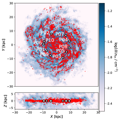
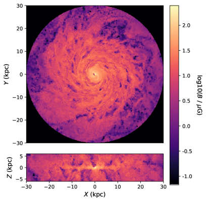
Figure 2: Left panel: Distribution of thermal electrons $n_{\mathrm{th}}$ in the disc midplane (top) and perpendicular to it (bottom) provided by the population synthesis model of Pellegrini & Reissl et al. (2019 sub.). Red dots represent the cluster population and black circles and white labels indicate the selected observer positions. Right panel: Corresponding magnetic field strength of the Au-6 galaxy (Grand et al., 2017) modified as outlined in Section 3.1.

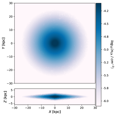
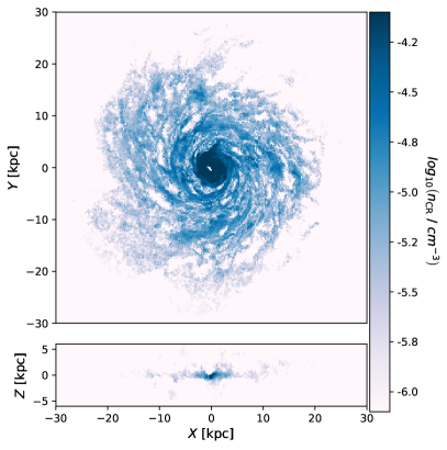
Figure 3: The same as Figure 3 for CR electron number densities $n_{\mathrm{CR}}$ for the CR1 model (left) and CR2 model (right) derived from Equation 25 (left panel) and Equation 28 (right panel), respectively.

3.1 Turbulent magnetic field

While MHD simulations provide the large-scale Galactic magnetic field they usually lack a small scale turbulent component due to insufficient numerical resolution. This component most likely follows a power-law, the exact parameters with regard to scale, magnitude, decay rates needs yet to be constrained (see e.g. Rand & Kulkarni, 1989; Minter & Spangler, 1996; Han et al., 2004; Sun et al., 2008, for details).

Especially, grid cells covering a regions of several $\mathrm{kpc}$ lack the small scale turbulent component. A more detailed modeling might require a subgrid approach but this is beyond the scope of this paper. Hence, we explore the influence of a turbulent magnetic field component added to our Galactic modeling and code testing setup by means of a Gaussian random field. We note that the original field of the Au-6 simulation already entails some turbulence and numerical noise. However, in the context of this paper we refer to the original Au-6 field as large scale field and to the Gaussian component as turbulent component.

A technique for generating Gaussian fluctuations by means of harmonics of a power-spectrum is presented in Martel (2005). However, this technique requires a resolution much smaller than Au-6. In order to reproduce the small-scale structures known from all-sky synchrotron emission and FR observations Haslam et al. (1981); Oppermann et al. (2012); Planck Collaboration et al. (2016b) we follow the procedure applied in Sun et al. (2008) and add to the large scale field $\vec{B}_{\rm MHD}(\vec{r})$ a Gaussian random component,

$$\vec{B}(\vec{r})=\vec{B}_{\rm MHD}(\vec{r})+b_{\rm\sigma_{b}}\vec{N}_{\rm\sigma_{B}}\,,$$ (24)

Here, $\vec{N}_{\rm\sigma_{B}}$ is the normalised direction with an angle between $\vec{N}_{\rm\sigma_{B}}$ and $\vec{B}_{\rm MHD}$ randomly sampled from a Gaussian with a variance of $\sigma_{B}=25^{\circ}$ selected to resemble observed small scale structures (see also Section 4.2). The magnitude of the Galactic turbulent field is estimated to be $\approx 2-3\ \rm{\mu G}$ (Sun et al., 2008). Thus, we sample from a Gaussian with $\sigma_{b}=2\ \rm{\mu G}$. We set $b_{\rm\sigma_{b}}=|\vec{B}_{\rm MHD}|$ in case of $b_{\rm\sigma_{b}}>|\vec{B}_{\rm MHD}|$. This is also in agreement with the finding of Han et al. (2004, 2006). They report that the Galactic regular field is of the same order of magnitude as the turbulent component. Here, we do not attempt to keep the field divergent free since this is not of relevance to RT simulation as outlined in the following sections.

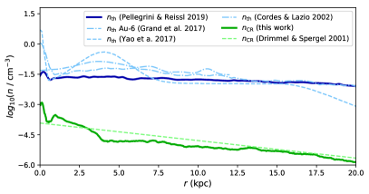
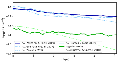
Figure 4: Left panel: Comparison of thermal electron number density $n_{\mathrm{th}}$ resulting from the population synthesis model of Pellegrini & Reissl et al. (2019 sub.) with the estimates presented in Yao et al. (2017) and Cordes & Lazio (2002) (blue lines) and a comparison of the parametrized CR1 electron density $n_{\mathrm{CR}}$ presented in Drimmel & Spergel (2001) with the CR2 mode derived in Section 3.2 (green lines). All quantities are averaged along the Galactic radius $r$ in the disc midplane $z=0\ \mathrm{kpc}$. Right panel: The same, but averaged along the $z$-direction at the solar radius $r=8\ \mathrm{kpc}$.

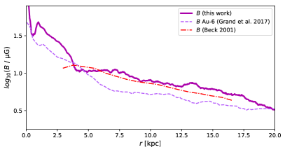
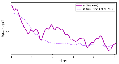
Figure 5: The same as Figure 5 for the magnetic field strength $B$ derived in Section 3.1 in comparison with the original Au-6 field strength (see Grand et al., 2017) and with the data presented in Beck (2001).

3.2 CR electron distribution

Cosmic ray electrons do not seem to be closely connected to the overall gas density structures of the galaxy (Strong et al., 2004b; Page et al., 2007). A smooth parameterisation of the CR electron distribution is suggested in Drimmel & Spergel (2001) and Page et al. (2007), respectively, as

$$n_{\rm CR_{1}}(x,y,z)=n_{\rm 0,CR}\exp\left(-\frac{r}{h_{\rm r}}\right)\cosh^{-2}\left(\frac{|z|}{h_{\rm z}}\right)\,.$$ (25)

Here, $x$, $y$, $z$ are Cartesian coordinates with their origin at the Galactic centre in units of $\mathrm{kpc}$ and $r=\sqrt{x^{2}+y^{2}}$ is the galactocentric radius. We apply a characteristic radius $h_{\rm r}=5\ \rm{kpc}$ and a scale height of $h_{\rm z}=1\ \rm{kpc}$ (Sun et al., 2008) for the CR distribution. The central CR electron density is taken to be the $n_{\rm 0,CR}=1.74\ 10^{-4}\rm{cm^{-3}}$ selected such that we ensure a typical value of $n_{\rm Earth}=6.4\ 10^{-5}\rm{cm^{-3}}$ for our solar neighbourhood at $r=8\ \rm{kpc}$ and $z=0\ \rm{kpc}$. Although, it remains to be seen if this density is typical for the entire Milky-Way. Here, we refer to this parametrization as the CR1 model.

Alternatively, the CR electron distribution can be derived from an equipartition argument. The magnetic energy stored in a cell of a certain volume is given by

$$u_{\rm B}=\frac{1}{8\pi}B^{2}\,.$$ (26)

The total energy density of the CR electrons can be estimated by integrating the particle energy $\gamma m_{\rm e}c^{2}$ over the CR distribution function. This results in

$$\begin{split}u_{\rm CR}=\int_{\gamma_{\rm min}}^{\gamma_{\rm max}}{\gamma m_{\rm e}c^{2}}N_{\rm CR}(\gamma)d\gamma\approx\qquad\qquad\qquad\qquad\\ \qquad\qquad\qquad\qquad n_{\rm CR}m_{\rm e}c^{2}\gamma_{\rm min}\frac{p-1}{p-2}\end{split}$$ (27)

given that $p\neq 2$ and $\gamma_{\rm min}\ll\gamma_{\rm max}$. We assume the magnetic field to be in equipartition with the CR electrons ($u_{\rm B}=u_{\rm CR}$). Consequently, the CR distribution function (Equation 16) scales approximately with the local magnetic field $B$ via:

$$n_{\rm CR_{2}}(x,y,z)\simeq\frac{B^{2}(x,y,z)(p-2)}{8\pi\gamma_{\rm min}(p-1)m_{\rm e}c^{2}}$$ (28)

We refer to this relation as the CR2 model as an alternative synchrotron RT test scenario for POLARIS.

The power law index $p$ as well as the lower cut off $\gamma_{\rm min}$ and upper cut off $\gamma_{\rm max}$ of the distribution function (see Equation 16) are also not well constrained galaxy-wide. The range between the cut offs is usually taken to be between the order of unity and several hundred (e.g. Ferland & Mushotzky, 1984; deKool & Begelman, 1989; Strong et al., 2011). In this work we apply a typical value of $\gamma_{\rm min}=4$ (see e.g Webber, 1998) and $\gamma_{\rm max}=300$, respectively, for the CR spectrum. Indeed, the exact value of the upper cut off is of minor relevance as long as $\gamma_{\rm max}\gg 1$ (compare Equation 17 and Equation 21).

In principle the power-law index $p$ may change dependent on the position within the galaxy. Observations suggested that $p$ varies with height $z$ (e.g. Miville-Deschênes et al., 2008) with lower values in the plane and large values toward the halo with a range of about $2-4$ (Bennett et al., 2003; Miville-Deschênes et al., 2008).

For our galaxy models we assume a fixed power-law index with a canonical value of $p=3$ (Rybicki & Lightman, 1979; Miville-Deschênes et al., 2008). Consequently, the maximal degree of linear polarisation that can be expected from synchrotron emission is $P_{\rm l}=0.75$ (see Equation 20).

4 Results and Discussion

With the above new features and extensions of POLARIS applied to the Au-6 galaxy, we now discuss in detail how the results compare to the observed characteristics of the Milky Way and of selected extragalactic systems.

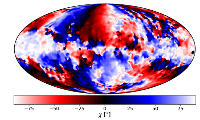
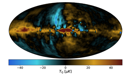
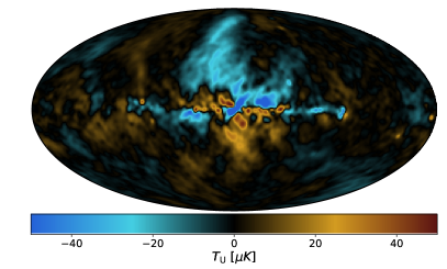
Figure 6: Top Row: Synchrotron emission at $734.8\ \mathrm{mm}$ (left panel) overlaid with polarisation vectors derived from the $1.0\ \mathrm{mm}$ polarisation observations (see Haslam et al., 1981, 1982, for details) and the orientation angles of the Galactic synchrotron polarisation (right panel) at $1.0\ \mathrm{mm}$ (see Equation 4). Bottom row: Corresponding $1.0\ \mathrm{mm}$ synchrotron Stokes Q map (left panel) and Stokes U map (right panel) (see Page et al., 2007; Hinshaw et al., 2009).

4.1 Galactic observables

The spatial distribution of the key input parameters necessary for computing realistic synchrotron emission maps is illustrated in Figures 3 and 3. We show cuts through the disc midplane and perpendicular to it. The thermal electron number density is presented in the left panel of Figure 3 based on the population synthesis model presented in Pellegrini & Reissl et al. (2019 sub.), while the right panel gives the magnetic field structure of the Au-6 galaxy (Grand et al., 2017) extended by a turbulent component, as discussed in Section 3.1. Magnetic field strength and thermal electrons clearly correlate and exhibit a characteristic spiral structure, as expected from extragalactic observations (e.g. Beck, 2001). The distribution of cosmic ray electrons, CR1 and CR2, as discussed in the previous section, is shown in Figure 3. Comparing both distributions one might expect more small-scale features in the synthetic synchrotron observations from model CR2.

A more quantitative view of these distributions is given in Figures 5 and 5, where we present the average radial profile in the disc midplane as well as the vertical profile out of the disc computed at the solar radius of $8\ \mathrm{kpc}$. The thermal electron distribution of the population synthesis model of Pellegrini & Reissl et al. (2019 sub.) (blue line) agrees well with the data of Yao et al. (2017) as well as with the the model of Cordes & Lazio (2002), with only small deviations close to the galactic centre and the very outer disc. As similar behavior is visible in the distribution of cosmic ray electrons (green line), which we compare to the parameterisation of Drimmel & Spergel (2001). In the range $2.5\ \mathrm{kpc}<r<17\ \mathrm{kpc}$ and $z<3\ \mathrm{kpc}$ our model is able to reproduce the existing data and other theoretical models very well in terms of the overall density of free electrons. We note that deviations in the galactic centre and in the outer parts of the disc contribute very little to the observed emission on the sky of an observer at the solar neighbourhood at $r\approx 8\ \mathrm{kpc}$ and $z\approx 0\ \mathrm{kpc}$ (Pakmor et al., 2018). Similar holds for the strengths of the magnetic field which enters our calculation of synchrotron emission and Faraday rotation. Our model very well reproduces the data presented by Beck (2001) in the disc midplane. However, our field is typically 10-20% stronger than the original magnetic field of the Au-6 galaxy (see Grand et al., 2017) because we add a turbulent component as introduced in Section 3.1.

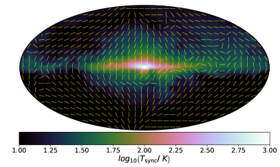
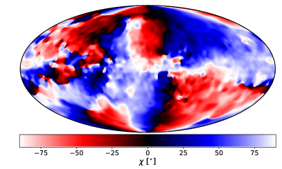
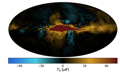
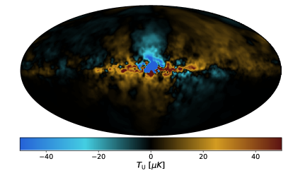
Figure 7: The same as Figure 6 but now for the synthetic emission resulting for the CR1 electron distribution (see Equation 25) as seen from the exemplary observes position P01.

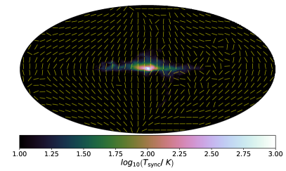
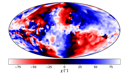
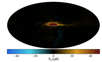
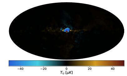
Figure 8: The same as Figure 7 for the CR2 electron distribution (see Equation 28) as seen from the exemplary observes position P01.

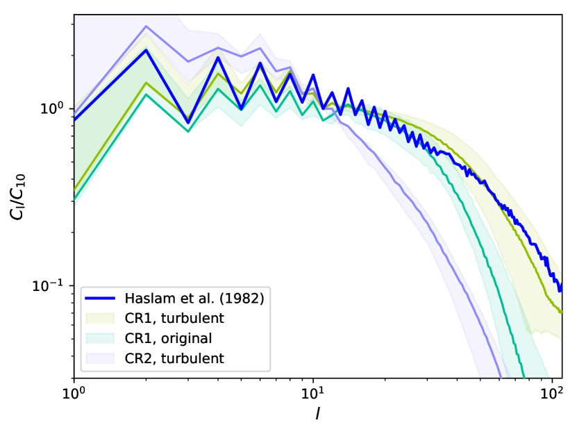
Figure 9: Multipole spectrum as a function of multipole moment $l$ of the synthetic all-sky synchrotron emission maps for the distinct observer positions resulting from the CR1 model with turbulent magnetic field component (yellow) CR1 model with the original Au-6 field (green) and the CR2 model with the turbulent field (purple). For comparison we plot the spectrum of the Haslam et al. (1982) map in blue. All spectra are normalised at $l=10$ for a better comparison. Solid lines are for the observer position P01 while the bands are the range of the spectra of the positions P02-P01.

4.2 Synchrotron emission and polarisation observations

The Haslam et al. (1981, 1982) all-sky map of the Galactic synchrotron emission at a wavelength of $734.8\ \mathrm{mm}$ still represents one of the most important radio surveys to this day. It is the standard which we use to validate our synthetic synchrotron emission maps generated with POLARIS. In addition, we include $1.0\ \mathrm{mm}$ data from the Wilkinson Microwave Anisotropy Probe (WMAP) sky survey (see Page et al., 2007; Hinshaw et al., 2009) to acquire Stokes Q, U, and orientation maps for polarisation comparisons. These maps of intensity as well as polarisation are shown in Figure 6.

To simulate all-sky maps of different observers position within the Milky Way like Au-6 galaxy we employ POLARIS in the mode of spherical detectors using the HEALPIX pixelation scheme at a wavelength of $734.8\ \mathrm{mm}$ as well as $1.0\ \mathrm{mm}$. We do so for ten distinct observer positions as indicated in the left panel of Figure 3. They lie in the disc midplane at $z=0\ \mathrm{pc}$ within a radius of about $8\ \mathrm{pc}\leq r\leq 10\ \mathrm{pc}$. To best mimic the conditions in the solar neighbourhood, we select the observers to be placed within a gas density cavity similar to the Local Bubble that defines our own Galactic environment (see e.g. Fuchs et al., 2009; Liu et al., 2017; Alves et al., 2018). Choosing the positions fully at random may accidentally result in an observer placed within or close to a molecular cloud. This would result in maps that are highly overshadowed by the contribution from very dense gas nearby contrary to what is observed.

As an example of the all-sky maps generated with a POLARIS RT calculation applying the CR1 model we show the result obtained for position P01 in Figure 7. The $734.8\ \mathrm{mm}$ synchrotron emission map (upper left corner) agrees well with the range of intensities found by Haslam et al. (1982) and presented in Figure 6. However, we have stronger emission towards the Galactic Centre. This is a result of the central peak in the magnetic field component of our Galactic model (see Figure 5). The vectors of linear polarisation match overall the ones of the WMAP probe indicating a toroidal field component in both the Milky Way as well as our Galactic model (see also Appendix C for a map with a purely toroidal field). Such a pattern is also known from dust polarisation observations (see Planck Collaboration et al., 2014). However, both observations and synthetic maps of orientation angle $\chi$ show values closer to $-45^{\circ}$ above the galactic centre and $45^{\circ}$ below the centre whereas one would have expected $\pm 90^{\circ}$ along the Galactic latitude for a purely toroidal field (compare Figure 14). We assume that this is because the signal does not probe the entire galaxy but is more dominated by the emission closer to the observer (see also the discussion about the effects of the Local Bubble by Alves et al., 2018). The same holds for the maps of the Stokes Q and U component. The magnitude of synthetic Q and U emission matches with the WMAP observations, but we overpredict the emission from the Galactic Centre.

In Figure 8 we show maps similar to Figure 7, however, now the synthetic emission is based on the CR2 model. The pattern of linear polarisation is very similar to the Milky Way (Figure 6) and to the CR2 model (Figure 7). Also the orientation map shows a similarly coherent polarisation. Comparing the lower panels of these figures reveals that the synchrotron emission in I, Q, and U, respectively, is underestimated by about one to two orders of magnitude throughout most of the galaxy.

To explore this further and to better understand the influence of the different model parameters on the resulting synchrotron maps we quantify the spatial distribution of the emission using a multipole expansion in spherical harmonics (see e.g. Pellegrini & Reissl et al., 2019 sub., for further details about this procedure). In Figure 9 we show the multipole spectrum obtained for the ten different observer positions (see Figure 3) in comparison to the one of the Haslam et al. (1982) maps for the CR1 and CR2 model, respectively, with and without a turbulent component. The amplitude characterises the amount of structure in the maps on different scales, going from large to small as the multipole moments $l$ increase from low to high values. We find that all synthetic spectra exhibit the typical saw-tooth pattern well known for our Milky-Way. Such a pattern can also bee seen in other tracers such as $H_{\alpha}$ (see e.g. Pellegrini & Reissl et al., 2019 sub.). As for synchrotron emission, the multipole spectrum of the smooth CR1 model derived from Drimmel & Spergel (2001) with an additional turbulent field agrees very well with the one of the original Haslam et al. (1981) map. There is only slight tendency for the synthetic maps to overestimate the fluctuations in the range ${20<l<50}$ while for $l>70$ we get a somewhat steeper slope. We note that a good match requires us to add a fluctuating magnetic field component to the relatively smooth magnetic field configuration in the underlying Au-6 galaxy. It follows a Gaussian modulation with $\sigma_{B}=25^{\circ}$ and $\sigma_{b}=2\ \rm{\mu G}$ (see Section 3.1 for definitions). We emphasise that these particular parameters may only apply in the context of this POLARIS CR1 test setup. Different galaxies may require a different choice of parameters. They may also be degenerate with a wide range of parameters leading to similar multipole fits. Furthermore, grid artifacts may enhance the small scale structure of the synthetic maps. However, exploring this range of degeneracy goes beyond the scope of this code paper.

When we take the magnetic field structure of Au-6 at face value and do not add a small-scale turbulent component, we still see a saw-tooth pattern for $l\leq 10$ for model CR1. However, the spectrum decays too quickly at larger $l$ indicating that the corresponding maps exhibit to little small-scale structure. We conclude that the presence of supersonic turbulence, which is ubiquitously observed in the Galactic interstellar medium and which is known to be one of the primary physical agents controlling the star formation process (Elmegreen & Scalo, 2004; Mac Low & Klessen, 2004; Klessen & Glover, 2016), is also important in determining the small-scale characteristics of the Galactic synchrotron emission.

Finally, we also plot the multipole model fit for CR2 with turbulent component in Figure 9. Yet again, we see a saw-tooth pattern pattern, but it is even less predominant and the spectrum decays even more rapidly with increasing $l$. Even with a turbulent magnetic field component, our particular CR2 model is not capable of reproducing the small-scale structures.

This may seem surprising at first sight, because CR2 exhibits much more structure than the smooth CR1 model based on Drimmel & Spergel (2001). Once again, emphasises the importance of the local environment for the observed synchrotron emission. The CR2 model has large patches with little to no free electrons. If the observer is placed within such a region, as we do in P01 to P10 to mimic the Local Bubble, then the immediate surrounding will contribute very little to the observed flux. In our case, this leads to too low emission at high galactic latitutes and towards the galactic anticentre. In addition, we find too little small-scale variations resulting in a steep decline of the angular power spectrum beyond $l\approx 10$.

We emphasise that all these findings concerning the lower emission of the CR2 model may only be true for our particular Galactic disc model. In general, the CR2 model may still be an viable alternative to the CR1 parametrization presented in Drimmel & Spergel (2001) considering other types of MHD simulations as future inputs for POLARIS.

4.3 Extragalactic observations and Faraday depolarisation

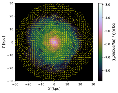
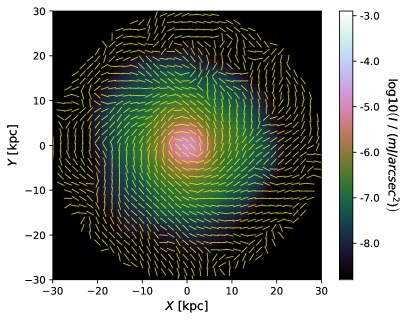
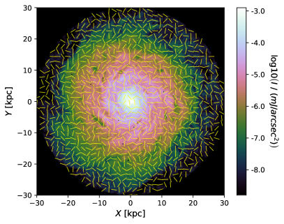
Figure 10: Synchrotron emission maps for a wavelength of $62\ \mathrm{mm}$ with a resolution of $0.15^{\prime\prime}$ (top left) and $15^{\prime\prime}$ (top right) and maps for a wavelength of $201\ \mathrm{mm}$ with a resolution of $0.15^{\prime\prime}$ (bottom left) and $15^{\prime\prime}$ (bottom right). The galaxy is at a distance of $3.5\ \mathrm{Mpc}$ and overlaid with normalised polarisation vectors. The vectors are rotated by $90^{\circ}$ to match the actual magnetic field direction.

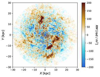
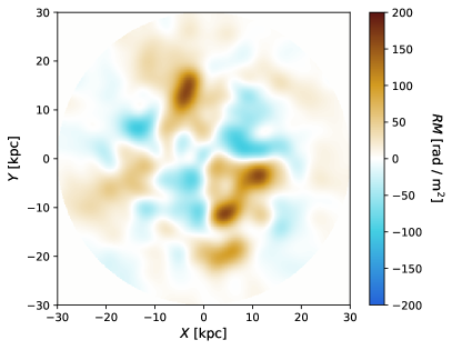
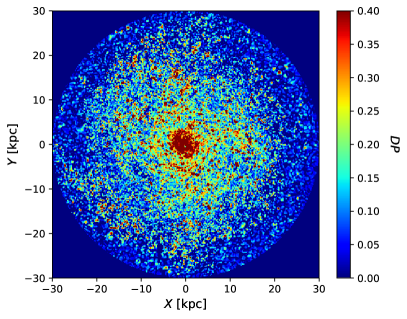
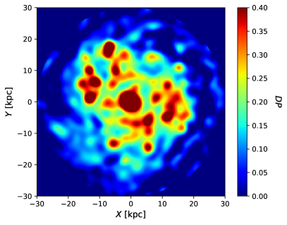
Figure 11: The same as Figure 10 for the Faraday RM (top panels) and the depolarisation fraction DP (bottom panels) as defined in Equation 15 with $\lambda_{1}=201\ \mathrm{mm}$ and $\lambda_{2}=62\ \mathrm{mm}$. Again, images on the left side have a resolution of $0.15^{\prime\prime}$, while the right side was smoothed to $15^{\prime\prime}$.

As part of the radiative transfer calculations that form the base of the emission maps discussed in the previous section POLARIS automatically produces the corresponding map of the Faraday rotation measure (RM). Arguing from the Stokes vector formalism, even a parallel magnetic field may not achieve the highest expected degree of linear polarisation (see Equation 20). The permanent mixing of the Q, U, and V component by means of FC and FR may lead to a depolarisation of radiation due to the additive nature of the Stokes vector. These depolarisation effects especially the Faraday rotation measures (RM) are extensively studied in Sokoloff et al. (1998) and observed in the nearby spiral galaxies IC 342, M51, and NGC 25, respectively, by Heesen et al. (2011a, b), Fletcher et al. (2011), and Beck (2015).

In order to test the POLARIS code for accurate predictions of depolarisation effects and RM in extragalactic objects, we produce similar observations with a face-on planar detector at a distance of $3.5\ \mathrm{Mpc}$ away from the CR1 model with turbulent magnetic field for wavelengths of $62\ \mathrm{mm}$, $201\ \mathrm{mm}$, and $734.8\ \mathrm{mm}$. Here, resolution effects are studied by smoothing the Stokes I, Q, and U maps with a Gaussian beam of $0.15^{\prime\prime}$ and $15^{\prime\prime}$, respectively. The later resolution is comparable to that of Fletcher et al. (2011) and Beck (2015).

We remind the reader that the density of thermal and cosmic ray electrons in the outskirts of the Au-6 galaxy model, i.e. for $r>15\ \mathrm{kpc}$, is higher than in the Milky Way (see Figure 5) and so the resulting synthetic maps may not provide a fully appropriate outside view onto the Milky Way.

Figure 10 presents the resulting emission maps at $62\ \mathrm{mm}$ and $201\ \mathrm{mm}$ for different resolutions overlaid with normalised polarisation vectors tracing the magnetic field direction. For $62\ \mathrm{mm}$ and $0.15^{\prime\prime}$ the polarisation is well ordered in the disc and centre regions with a magnetic field following the spiral pattern, but the polarisation becomes increasingly disordered towards the outer edge of the disc. For the $15^{\prime\prime}$ smoothed map, the toroidal component becomes even more apparent. Such a pattern seems to be a common feature in radio and optical spiral disc observations (e.g. Fendt et al., 1998; Soida et al., 2002; Fletcher et al., 2011; Beck, 2015; Frick et al., 2016) indicating again a strong toroidal field with a non-negligible turbulent component. Observing at $201\ \mathrm{mm}$ (or even $734.8\ \mathrm{mm}$) leads to severe perturbations of this coherent pattern even in the centre, since FR becomes increasingly dominant (see also Equation 13 and Figure 11). Here, synchrotron polarisation does no longer allow to accurately trace the magnetic field morphology at longer wavelengths. A similar trend was observed in the polarisation pattern of M51 for $62\ \mathrm{mm}$ and $201\ \mathrm{mm}$ as presented in Fletcher et al. (2011). In contrast to the $201\ \mathrm{mm}$ maps in Fig. 10, in M51 observations the correlation between the spiral arms and the polarisation patters is not completely lost. However, M51 has only two spiral arms with large inter-arm regions while the Au-6 is much more tightly wound. Hence, the $201\ \mathrm{mm}$ polarisation pattern in Fig. 10 can no longer clearly be attributed to any particular spiral even in our high resolution map.

The corresponding map of the Faraday RM is depicted in the top panels of Figure 11. The spatial distribution as well as the magnitude of the effect (up to $\pm 200\ \mathrm{rad/m^{2}}$) match well with the expectations from a similar high-resolution RM study based on the original AU-6 MHD (Pakmor et al., 2018) and with what is known from extragalactic observations (e.g. Heesen et al., 2011a; Fletcher et al., 2011; Beck, 2015). Faraday rotation can be the result of density fluctuations within the thermal electron distribution as well as in the magnitude and orientation of the magnetic field. Because the magnetic field structure of the Au-6 galaxy is rather regular, even when adding a turbulent component, we conclude that the changes in the magnitude of RM seen in the top panels of Figure 11 is mostly due to fluctuations in the thermal electron density. However, this clearly deserves further investigation. Any follow-up studies would also need to take the contribution of the halo field to the total RM into account, which is an effect that we neglect here.

In the bottom panels of Figure 11 we also show a map of the depolarisation fraction DP, as defined in Equation 15, using $\lambda_{1}=201\ \mathrm{mm}$ and $\lambda_{2}=62\ \mathrm{mm}$ as well as a constant spectral index of $\alpha=1$. The magnitude varies mostly between $0$ and $0.4$ with peak values up to $0.8$ for both the $0.15^{\prime\prime}$ and the $15^{\prime\prime}$ maps. This result concurs with the maps presented in Beck (2015), Fletcher et al. (2011) and Heesen et al. (2011b), although the latter authors also report peak values up to unity. Our map does not particularly resemble the spiral structure of the emission with most of the DP occurring in distinct spots. We note that, these spots are connected to the most ionizing cluster regions of the population synthesis model of Pellegrini & Reissl et al. (2019 sub.). The lack of correlation between density structures and DP is also consistent with observations e.g. with the M51 DP map presented in Fletcher et al. (2011).

We emphasize that the native resolution of our synthetic extragalactic observations corresponds to $0.15\ \mathrm{{}^{\prime\prime}}$, which is a hundred times better than the data presented in Heesen et al. (2011a, b), Fletcher et al. (2011), or Beck (2015), respectively. This demonstrates the high quality of the data coming from the POLARIS RT simulations.

5 Summary

In this paper, we presented an updated and extended version of the polarisation radiative transfer code POLARIS. The new code solves the full four Stokes parameters matrix equation of the radiative transfer problem in order to create synthetic synchrotron emission maps including polarisation, Faraday conversion and Faraday rotation. POLARIS can be used to generate synthetic observations based on multi-physics numerical simulations as input running on the native grids of all major astrophysical MHD codes.

As a case study, we tested the accuracy and predictive capability of the POLARIS code through a set of radiative transfer simulations based on the Auriga cosmological MHD zoom simulation project Grand et al. (2017). The selected galaxy, Au-6, is an analog of the Milky Way. We modified it by employing the star cluster population synthesis model WARPFIELD-POP presented by (Pellegrini & Reissl et al., 2019 sub.) to produce a more realistic distribution of thermal electrons and by adding a turbulent component to the original magnetic field. To explore the impact of cosmic ray electrons, we investigated to different approaches based on exiting models. The radiative transfer simulations we ran explored the influence of the different post-processing steps, electron distributions, as well as observational conditions of the Auriga galaxy on synchrotron observables. We focused our attention on those wavelengths that are most commonly used in observations of Galactic magnetic fields ($1\ \mathrm{mm}$ to $730\ \mathrm{mm}$). Our synthetic synchrotron all-sky maps match well with actual observations both in magnitude and structure. Furthermore, we produced and examined mock observations of extragalactic systems, which show familiar patterns in polarisation, Faraday rotation measure, and depolarisation. Altogether, we demonstrated that POLARIS is a tool that reliable computes synchrotron emission, polarisation, the internal and external depolarisation and Faraday rotation effects. It can produce reliable all-sky maps for a fictitious observer within a galaxy and it can create images of galaxies as seen from far away. POLARIS is a highly versatile radiative transfer code that can be used for the detailed comparison with Galactic and extragalactic observations.

We summarise our scientific findings as follows: (i) Different methods to derive Galactic cosmic ray electron distributions, based on a simple parametrisation and on energy equipartition, reproduce the observed synchrotron polarisation pattern. However, the equipartition approach seems to underestimate the total amount of synchrotron emission. (ii) The presence of a turbulent magnetic field component is required to reproduce the observed Galactic small-scale structures of the synchrotron emission. (iii) Our radiative transfer simulations indicate that the observed Galactic synchrotron emission depends strongly on the actual position within the Milky Way disc. (iv) The depolarisation pattern observed in our synthetic galaxy by an observer far away is largely accounted for by Faraday rotation, its small-scale features are mostly dominated by the thermal electron distribution.

In a series of forthcoming papers we plan to utilise POLARIS to further minimise observed ambiguities in magnetic field measurements by means of dust polarisation (e.g. Reissl et al., 2014, 2018) or Zeeman effect Brauer et al. (2017b, a); Reissl et al. (2018). The set of unique polarisation features unified in a single code has also the potential to address open questions concerning the separation the CMB measurements from the pollution of dust and synchrotron polarisation coming from our own Milky-Way.

Appendix A Error estimation and code limitations

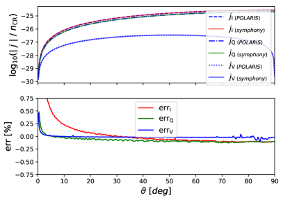
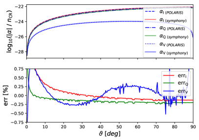
Figure 12: Left column: Fitted emission coefficient $j_{\mathrm{I}}$ for intensity, $j_{\mathrm{Q}}$ for linear polarisation, and $j_{\mathrm{V}}$ for circular polarisation as they are implemented in POLARIS over angle $\vartheta$ in comparison with exact integral solutions provided by the SYMPHONY code. Here, the parameters are $\lambda=734.8\ \mathrm{mm}$, $B=30\ \mathrm{G}$, power-law index $p=3$, $\gamma_{\mathrm{min}}=4$, and $\gamma_{\mathrm{min}}=300$. The error is defined to be $\mathrm{err}=1-j_{(\mathrm{{POLARIS}})}/j_{(\mathrm{{SYMPHONY}})}$. Right column: The same as the left column for the corresponding emission coefficients $\alpha_{\mathrm{I}}$, $\alpha_{\mathrm{Q}}$, and $\alpha_{\mathrm{U}}$, respectively. Note, that all Q coefficients are negative and all V coefficients do change their sign from positive to negative values for $\vartheta>90^{\circ}$.

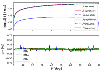
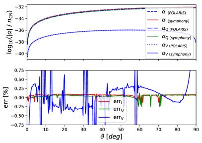
Figure 13: The same as Figure 13 for $B=3\ \mathrm{mG}$.

In this section we explore the limitations of the applied fit functions in comparison with the exact integral solutions of the coefficients of synchrotron emission, absorption, Faraday conversion (FC), and Faraday rotation (FR). For that we consider an maximum error of $1\ \%$ to be acceptable for the POLARIS implementation. This limits the range of wavelength $\lambda$ available for synthetic observations to ${10^{2}<\lambda_{\rm c}/\lambda<10^{9}}$ (see Equation 10 for the definition of $\lambda_{\rm c}$). In turn the range of the energy spectrum is given by ${\gamma_{\rm min}^{2}\ll\lambda_{\rm c}/\lambda<\gamma_{\rm max}^{2}}$ (see Pandya et al., 2016, for details). We note that the upper limit is less strict as long as the ratio ${\lambda_{\rm c}/\lambda}$ is of the same order as $\gamma_{\rm max}^{2}$.

Errors up to $35\ \%$ are reported in Pandya et al. (2016). However, these uncertainties are given for a magnitude of the magnetic field in the order of $\approx 10\ \mathrm{G}$ and for small values of $\vartheta$. Indeed, this rather high field strength is far beyond values typical for the Milky Way where we can expect values of about $6\ \mathrm{\mu G}$ (Strong et al., 2000) in our local environment and up to $1\ \mathrm{mG}$ (Yusef-Zadeh et al., 1996) near the Galactic Centre. A similar range of field strengths can be expected for other spiral galaxies (Niklas, 1995).

We compare the integral solutions calculated with the SYMPHONY code (Pandya et al., 2016) to the fit functions as they are implemented in POLARIS. Here, we find for $B\ll 1\ \mathrm{G}$ the absorption and emission coefficients are less prone to errors even for smaller values of the angle $\vartheta$ (compare Figures 13 and 13). Consequently, we can apply the fit functions throughout the parameter space of the Milky Way model presented in this paper.

We report some irregularities between fit functions and exact integral solutions for a lower cut-off of $\gamma_{\mathrm{min}}\neq 1$. Indeed, the fit functions in SYMPHONY do not apply for $\gamma_{\mathrm{min}}>1$. Hence, we corrected Equations 17 and 21 by an additional factor of $\gamma_{\mathrm{min}}^{1-p}$ in order to provide general solutions for any $\gamma_{\mathrm{min}}>1$.

We also find an offset between the integral solution and the fit functions of the absorption coefficient $\alpha_{\mathrm{Q}}$ of about $4\ \%$ being constant over a large parameter range. Assuming the integral solutions to be correct we multiply an additional factor of $996/1000$ to decrease this offset in Equation 22.

A similar problem occurs for the absorption coefficient $\alpha_{\mathrm{V}}$. Here, the offset depends on the angle $\vartheta$ and exceeds the demanded $1\ \%$ error limit over a wide range of $\vartheta$. We apply an additional correction function to Equation 23 defined to be

$$k_{\mathrm{V}}(\vartheta)=\begin{cases}0.9914+0.0075\times\vartheta^{11/12}&\mbox{if }\vartheta\leq 0.8034\\ 0.9919+0.0013/\sin(0.0048+\vartheta)&\mbox{else}\end{cases}\,.$$ (A1)

In Figures 13 and 13 we plot the emission and absorption as well as the errors between the implementation in SYMPHONY and POLARIS. We attribute the noise in the error plots to the integration scheme of SYMPHONY. Indeed, for $B\leq 3\ \mathrm{mG}$ the implemented fit functions in POLARIS agree very well with the integral solutions of SYMPHONY. The only exception is the corrected absorption coefficient of circular polarisation $\alpha_{\mathrm{V}}$. The correction function pushes the error bellow $0.75\ \%$ except for angles $\vartheta<3^{\circ}$ and $\vartheta>87^{\circ}$, respectively. However, we consider this error acceptable since $\alpha_{\mathrm{V}}\rightarrow 0$ much faster as $\alpha_{\mathrm{I}}$ and $\alpha_{\mathrm{Q}}$, respectively, in this range and contributes only marginally to the total RT process.

Furthermore, the implemented FR and FC coefficients are only valid in a regime with electron temperatures of $T_{\mathrm{e}}\ll 10^{9}-10^{10}\ \mathrm{K}$. In a more extreme environment such as black hole accretion flows (see e.g. Rajesh & Mukhopadhyay, 2010; Chael et al., 2017) the coefficients in Equation 12 and Equation 11 need to be modified by some additional correction factors as discussed e.g. in Shcherbakov (2008) or Dexter (2016).

Appendix B Numerical solver and adaptive step size

Implemented in the POLARIS code is a Runge-Kutta-Fehlberg (RFK45) solver in order to provide a high accuracy solution to the matrix RT problem. This method uses an inbuilt step size $d\ell$ correction to keep the error below a certain threshold $\epsilon$. Here, the solver compares the fourth order Runge-Kutta solution $X_{I,Q,U,V,4}$ for any of the Stokes component with the fifth order solution $X_{I,Q,U,V,5}$ by

$$\epsilon_{\mathrm{I,Q,U,V}}=\left|\frac{X_{I,Q,U,V,4}-X_{I,Q,U,V,5}}{\epsilon_{\mathrm{err}}X_{I,Q,U,V,5}+\epsilon_{\mathrm{abs}}}\right|\,.$$ (B1)

By default the relative error is implemented in POLARIS to be ${\epsilon_{\mathrm{err}}=10^{-8}}$ with an absolute error of ${\epsilon_{\mathrm{abs}}=10^{-30}}$ . The RFK45 method solves the RT problem usually within a few steps per cell. However, in RT with synchrotron polarisation we have to handle the permanent transfer between the Q, U, and V components via the FR and FC coefficients. Consequently, the system of differential equations oscillates between these Stokes parameters of polarisation. A step size that is only based on the I parameter might be too large for the other Stokes parameter and can lead to the forbidden condition of $I<p_{\mathrm{t}}$. Hence, we account for this case by calculating four separate thresholds $\epsilon_{\mathrm{I,Q,U,V}}$ for each of the Stokes parameters. The final threshold is then

$$\epsilon=\min\left(\epsilon_{\mathrm{I}},\epsilon_{\mathrm{Q}},\epsilon_{\mathrm{U}},\epsilon_{\mathrm{V}}\right)\,.$$ (B2)

For the case of $\epsilon>1$ a smaller step size $d\ell_{\mathrm{new}}$ for the current integration step needs to be determined according to

$$d\ell_{\mathrm{new}}=\min\left(\frac{1}{10}\times d\ell_{\mathrm{old}},\frac{1}{4}d\ell_{\mathrm{old}}\epsilon^{-0.2}\right)\,.$$ (B3)

Otherwise, for $\epsilon\leq 1$ the integration step $d\ell$ is sufficiently small to solve the equation system of synchrotron RT within the defined error limits. Finally, the simulations stops when a all rays have reached the detector.

We note that, under rare conditions the solver may still need several thousand steps within a singles cell. In order to circumvent this problem we implemented an alternative solver scheme. When the number of steps per cell exceeds a number of $5\times 10^{5}$ we separate the RT problem. Since the FR and FC coefficients usually require the smaller $d\ell$ we write the system of equations as

$$\frac{d}{d\ell}\vec{S}=-\left(\hat{K}_{\alpha}+\hat{K}_{\kappa}\right)\vec{S}+\vec{J}\,,$$ (B4)

where

$$\hat{K}_{\alpha}=\begin{pmatrix}\alpha_{\rm I}&\alpha_{\rm Q}&0&\alpha_{\rm V}\\ \alpha_{\rm Q}&\alpha_{\rm I}&0&0\\ 0&0&\alpha_{\rm I}&0\\ \alpha_{\rm V}&0&0&\alpha_{\rm I}\end{pmatrix}$$ (B5)

is the absorption matrix and

$$\hat{K}_{\kappa}=\begin{pmatrix}0&0&0&0\\ 0&0&\kappa_{\rm V}&0\\ 0&-\kappa_{\rm V}&0&\kappa_{\rm Q}\\ 0&0&-\kappa_{\rm Q}&0\end{pmatrix}$$ (B6)

is the Faraday matrix. Now, we solve only the RT problem with $\hat{K}_{\alpha}$ by means of the RFK45 solver and $\epsilon_{\mathrm{I}}$ leading to a step size $d\ell_{\mathrm{I}}$ and finally to a solution of $\vec{S}_{\alpha}$ ignoring FR and FC effects. For the Faraday part of the equation we make use of the analytically solution derived by Dexter (2016). Considering only $\hat{K}_{\kappa}$ the oscillation of the Stokes polarisation parameters Q, U, and V by means of Faraday mixing can analytically be calculated as

$$Q_{\kappa}=\frac{\kappa_{Q}}{\kappa^{2}}\left(j_{Q}\kappa_{Q}+j_{V}\kappa_{V}\right)d\ell_{\mathrm{I}}+\frac{\kappa_{V}}{\kappa^{3}}\left(j_{V}\kappa_{Q}+j_{Q}\kappa_{V}\right)\sin\left(\kappa d\ell_{\mathrm{I}}\right)-\frac{j_{U}\kappa_{V}}{\kappa^{2}}\left[1-\cos\left(\kappa d\ell_{\mathrm{I}}\right)\right]\,,$$ (B7)

$$U_{\kappa}=\frac{j_{Q}\kappa_{V}-j_{V}\kappa_{Q}}{\kappa^{2}}\left[1-\cos\left(\kappa d\ell_{\mathrm{I}}\right)\right]+\frac{j_{U}}{\kappa}\sin\left(\kappa d\ell_{\mathrm{I}}\right)\,,$$ (B8)

and

$$V_{\kappa}=\frac{\kappa_{V}}{\kappa^{2}}\left(j_{Q}\kappa_{Q}+j_{V}\kappa_{V}\right)d\ell_{\mathrm{I}}+\frac{\kappa_{V}}{\kappa^{3}}\left(j_{Q}\kappa_{V}+j_{V}\kappa_{Q}\right)\sin\left(\kappa d\ell_{\mathrm{I}}\right)+\frac{j_{U}\kappa_{Q}}{\kappa^{2}}\left[1-\cos\left(\kappa d\ell_{\mathrm{I}}\right)\right]$$ (B9)

with $\kappa^{2}=\kappa_{Q}^{2}+\kappa_{U}^{2}$. This second set of equations results in a solution of $\vec{S}_{\kappa}=(0,Q_{\kappa},U_{\kappa},V_{\kappa})^{T}$. The final solution is then simply ${\vec{S}=\vec{S}_{\alpha}+\vec{S}_{\kappa}}$. However, this approach is far less accurate than solving the full matrix equation. In extreme tests with electron densities of $n_{\mathrm{CR}}>10^{5}\ \mathrm{cm^{-2}}$ and magnetic fields of $B>5\ \mathrm{mG}$ the alternative solver scheme starts to kick in and we can get errors up to $5\ \%-10\ \%$ per cell. However, we consider this error range still to be acceptable as long as the number of grid cells with extreme conditions is sufficiently small enough compared to the total number of grid cells. Furthermore, electron densities up to $10^{5}\ \mathrm{cm^{-2}}$ and a field strength in the order of $\mathrm{mG}$ are rather untypical ISM conditions.

As a last fail-save we skip certain cells completely and jump to the next one when the amount of required RKF45 solver steps exceeds $10^{7}$. Splitting of RT matrices and limiting the maximal amount of solver steps allows the POLARIS code to terminate in any case and within a reasonable time frame. We note, that none of these implemented fail-saves kick in for the Milky Way model of (Pellegrini & Reissl et al., 2019 sub.) utilised in this paper.

Appendix C An idealised toroidal field model

Both, observations as well as modeled synchrotron all-sky polarisation maps discussed in this paper appear to be strongly controlled by a toroidal magnetic field component. Hence, we provide a polarisation map of a purely toroidal field in Figure 14 projected on a healpix sphere for comparison. The map is created with POLARIS assuming constant densities and a perfectly polarised emission perpendicular to the field direction without any absorption. We note, that a purely toroidal field would posses a quadrupole-like symmetry with an orientation of the linear polarisation vectors close to $\pm 90^{\circ}$ along the galactic longitude as well as latitude.

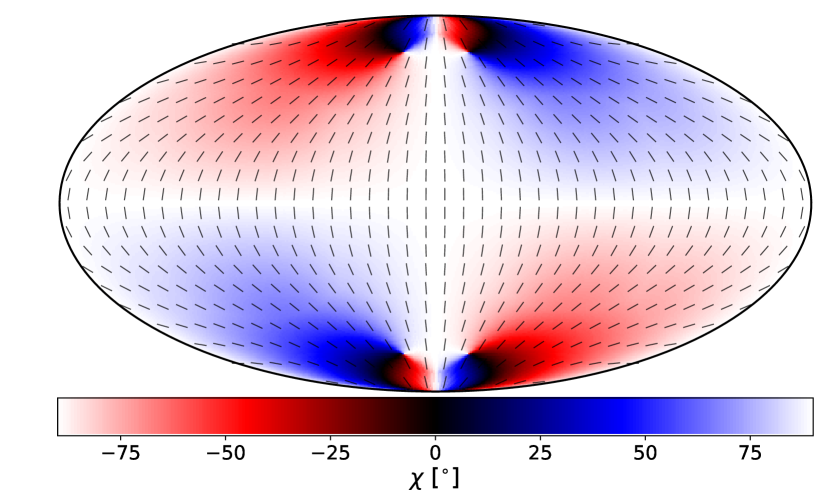
Figure 14: All-sky healpix projection of a purely toroidal magnetic field.

References

- Alves et al. (2018) Alves, M. I. R., Boulanger, F., Ferrière, K., & Montier, L. 2018, A&A, 611, L5, doi: 10.1051/0004-6361/201832637
- Andersson et al. (2015) Andersson, B.-G., Lazarian, A., & Vaillancourt, J. E. 2015, ARA&A, 53, 501, doi: 10.1146/annurev-astro-082214-122414
- Baczynski et al. (2015) Baczynski, C., Glover, S. C. O., & Klessen, R. S. 2015, MNRAS, 454, 380, doi: 10.1093/mnras/stv1906
- Baes et al. (2011) Baes, M., Verstappen, J., De Looze, I., et al. 2011, ApJS, 196, 22, doi: 10.1088/0067-0049/196/2/22
- Beck et al. (2016) Beck, M. C., Beck, A. M., Beck, R., et al. 2016, J. Cosmology Astropart. Phys, 5, 056, doi: 10.1088/1475-7516/2016/05/056
- Beck (2001) Beck, R. 2001, Space Sci. Rev., 99, 243
- Beck (2015) —. 2015, A&A, 578, A93, doi: 10.1051/0004-6361/201425572
- Bennett et al. (2003) Bennett, C. L., Hill, R. S., Hinshaw, G., et al. 2003, ApJS, 148, 97, doi: 10.1086/377252
- Brauer et al. (2017a) Brauer, R., Wolf, S., & Flock, M. 2017a, A&A, 607, A104, doi: 10.1051/0004-6361/201731140
- Brauer et al. (2016) Brauer, R., Wolf, S., & Reissl, S. 2016, A&A, 588, A129, doi: 10.1051/0004-6361/201527546
- Brauer et al. (2017b) Brauer, R., Wolf, S., Reissl, S., & Ober, F. 2017b, A&A, 601, A90, doi: 10.1051/0004-6361/201629001
- Chael et al. (2017) Chael, A. A., Narayan, R., & Saḑowski, A. 2017, MNRAS, 470, 2367, doi: 10.1093/mnras/stx1345
- Chandrasekhar & Fermi (1953) Chandrasekhar, S., & Fermi, E. 1953, ApJ, 118, 113, doi: 10.1086/145731
- Cordes & Lazio (2002) Cordes, J. M., & Lazio, T. J. W. 2002, ArXiv Astrophysics e-prints
- Crutcher (1999) Crutcher, R. M. 1999, ApJ, 520, 706, doi: 10.1086/307483
- Crutcher et al. (1993) Crutcher, R. M., Troland, T. H., Goodman, A. A., et al. 1993, ApJ, 407, 175, doi: 10.1086/172503
- deAvillez & Breitschwerdt (2005) deAvillez, M. A., & Breitschwerdt, D. 2005, A&A, 436, 585, doi: 10.1051/0004-6361:20042146
- deKool & Begelman (1989) deKool, M., & Begelman, M. C. 1989, ApJ, 345, 135, doi: 10.1086/167887
- Dexter (2016) Dexter, J. 2016, MNRAS, 462, 115, doi: 10.1093/mnras/stw1526
- Drimmel & Spergel (2001) Drimmel, R., & Spergel, D. N. 2001, ApJ, 556, 181, doi: 10.1086/321556
- Dullemond (2012) Dullemond, C. P. 2012, RADMC-3D: A multi-purpose radiative transfer tool, Astrophysics Source Code Library. http://ascl.net/1202.015
- Elmegreen & Scalo (2004) Elmegreen, B. G., & Scalo, J. 2004, ARA&A, 42, 211, doi: 10.1146/annurev.astro.41.011802.094859
- Enßlin (2003) Enßlin, T. A. 2003, A&A, 401, 499, doi: 10.1051/0004-6361:20030162
- Enßlin et al. (2017) Enßlin, T. A., Hutschenreuter, S., Vacca, V., & Oppermann, N. 2017, Phys. Rev. D, 96, 043021, doi: 10.1103/PhysRevD.96.043021
- Ercolano et al. (2003) Ercolano, B., Barlow, M. J., Storey, P. J., & Liu, X.-W. 2003, MNRAS, 340, 1136, doi: 10.1046/j.1365-8711.2003.06371.x
- Fauvet et al. (2012) Fauvet, L., Macías-Pérez, J. F., Jaffe, T. R., et al. 2012, A&A, 540, A122, doi: 10.1051/0004-6361/201016349
- Federrath et al. (2010) Federrath, C., Banerjee, R., Clark, P. C., & Klessen, R. S. 2010, ApJ, 713, 269, doi: 10.1088/0004-637X/713/1/269
- Fendt et al. (1998) Fendt, C., Beck, R., & Neininger, N. 1998, A&A, 335, 123
- Ferland & Mushotzky (1984) Ferland, G. J., & Mushotzky, R. F. 1984, ApJ, 286, 42, doi: 10.1086/162574
- Fletcher et al. (2011) Fletcher, A., Beck, R., Shukurov, A., Berkhuijsen, E. M., & Horellou, C. 2011, MNRAS, 412, 2396, doi: 10.1111/j.1365-2966.2010.18065.x
- Frick et al. (2016) Frick, P., Stepanov, R., Beck, R., et al. 2016, A&A, 585, A21, doi: 10.1051/0004-6361/201526796
- Fuchs et al. (2009) Fuchs, B., Breitschwerdt, D., de Avillez, M. A., & Dettbarn, C. 2009, Space Sci. Rev., 143, 437, doi: 10.1007/s11214-008-9427-z
- Gatto et al. (2015) Gatto, A., Walch, S., Low, M.-M. M., et al. 2015, MNRAS, 449, 1057, doi: 10.1093/mnras/stv324
- Gatto et al. (2017) Gatto, A., Walch, S., Naab, T., et al. 2017, MNRAS, 466, 1903, doi: 10.1093/mnras/stw3209
- Gent et al. (2013) Gent, F. A., Shukurov, A., Fletcher, A., Sarson, G. R., & Mantere, M. J. 2013, MNRAS, 432, 1396, doi: 10.1093/mnras/stt560
- Girichidis et al. (2018) Girichidis, P., Naab, T., Hanasz, M., & Walch, S. 2018, MNRAS, 479, 3042, doi: 10.1093/mnras/sty1653
- Girichidis et al. (2016) Girichidis, P., Walch, S., Naab, T., et al. 2016, MNRAS, 456, 3432, doi: 10.1093/mnras/stv2742
- Glover & Clark (2012) Glover, S. C. O., & Clark, P. C. 2012, MNRAS, 421, 116, doi: 10.1111/j.1365-2966.2011.20260.x
- Glover et al. (2010) Glover, S. C. O., Federrath, C., Mac Low, M.-M., & Klessen, R. S. 2010, MNRAS, 404, 2, doi: 10.1111/j.1365-2966.2009.15718.x
- Gordon et al. (2001) Gordon, K. D., Misselt, K. A., Witt, A. N., & Clayton, G. C. 2001, ApJ, 551, 269, doi: 10.1086/320082
- Grand et al. (2017) Grand, R. J. J., Gómez, F. A., Marinacci, F., et al. 2017, MNRAS, 467, 179, doi: 10.1093/mnras/stx071
- Grand et al. (2018a) Grand, R. J. J., Bustamante, S., Gómez, F. A., et al. 2018a, MNRAS, 474, 3629, doi: 10.1093/mnras/stx3025
- Grand et al. (2018b) Grand, R. J. J., Helly, J., Fattahi, A., et al. 2018b, ArXiv e-prints. https://arxiv.org/abs/1804.08549
- Gressel et al. (2013) Gressel, O., Elstner, D., & Ziegler, U. 2013, A&A, 560, A93, doi: 10.1051/0004-6361/201322349
- Haid et al. (2018) Haid, S., Walch, S., Seifried, D., et al. 2018, MNRAS, 478, 4799, doi: 10.1093/mnras/sty1315
- Han (2008) Han, J. L. 2008, Nuclear Physics B Proceedings Supplements, 175, 62, doi: 10.1016/j.nuclphysbps.2007.10.010
- Han et al. (2004) Han, J. L., Ferriere, K., & Manchester, R. N. 2004, ApJ, 610, 820, doi: 10.1086/421760
- Han et al. (2006) Han, J. L., Manchester, R. N., Lyne, A. G., Qiao, G. J., & van Straten, W. 2006, ApJ, 642, 868, doi: 10.1086/501444
- Harries (2014) Harries, T. 2014, TORUS: Radiation transport and hydrodynamics code, Astrophysics Source Code Library. http://ascl.net/1404.006
- Haslam et al. (1981) Haslam, C. G. T., Klein, U., Salter, C. J., et al. 1981, A&A, 100, 209
- Haslam et al. (1982) Haslam, C. G. T., Salter, C. J., Stoffel, H., & Wilson, W. E. 1982, A&AS, 47, 1
- Heesen et al. (2011a) Heesen, V., Beck, R., Krause, M., & Dettmar, R.-J. 2011a, A&A, 535, A79, doi: 10.1051/0004-6361/201117618
- Heesen et al. (2011b) Heesen, V., Rau, U., Rupen, M. P., Brinks, E., & Hunter, D. A. 2011b, ApJ, 739, L23, doi: 10.1088/2041-8205/739/1/L23
- Hennebelle (2018) Hennebelle, P. 2018, A&A, 611, A24, doi: 10.1051/0004-6361/201731071
- Hennebelle & Iffrig (2014) Hennebelle, P., & Iffrig, O. 2014, A&A, 570, A81, doi: 10.1051/0004-6361/201423392
- Heyvaerts et al. (2013) Heyvaerts, J., Pichon, C., Prunet, S., & Thiébaut, J. 2013, MNRAS, 430, 3320, doi: 10.1093/mnras/stt135
- Higdon (1979) Higdon, J. C. 1979, ApJ, 232, 113, doi: 10.1086/157270
- Hill et al. (2012) Hill, A. S., Joung, M. R., Mac Low, M.-M., et al. 2012, ApJ, 750, 104, doi: 10.1088/0004-637X/750/2/104
- Hinshaw et al. (2009) Hinshaw, G., Weiland, J. L., Hill, R. S., et al. 2009, ApJS, 180, 225, doi: 10.1088/0067-0049/180/2/225
- Huang & Shcherbakov (2011) Huang, L., & Shcherbakov, R. V. 2011, MNRAS, 416, 2574, doi: 10.1111/j.1365-2966.2011.19207.x
- Iacobelli et al. (2013) Iacobelli, M., Haverkorn, M., Orrú, E., et al. 2013, A&A, 558, A72, doi: 10.1051/0004-6361/201322013
- Jaffe et al. (2010) Jaffe, T. R., Leahy, J. P., Banday, A. J., et al. 2010, MNRAS, 401, 1013, doi: 10.1111/j.1365-2966.2009.15745.x
- Jansky (1933) Jansky, K. G. 1933, Popular Astronomy, 41, 548
- Jones & Hardee (1979) Jones, T. W., & Hardee, P. E. 1979, ApJ, 228, 268, doi: 10.1086/156843
- Jones & Odell (1977) Jones, T. W., & Odell, S. L. 1977, ApJ, 214, 522, doi: 10.1086/155278
- Joung & Mac Low (2006) Joung, M. K. R., & Mac Low, M.-M. 2006, ApJ, 653, 1266, doi: 10.1086/508795
- Juvela (1999) Juvela, M. 1999, in The Physics and Chemistry of the Interstellar Medium, ed. V. Ossenkopf, J. Stutzki, & G. Winnewisser, 220
- Juvela & Padoan (2003) Juvela, M., & Padoan, P. 2003, A&A, 397, 201, doi: 10.1051/0004-6361:20021433
- Juvela et al. (2018) Juvela, M., Guillet, V., Liu, T., et al. 2018, ArXiv e-prints. https://arxiv.org/abs/1809.00864
- Kiepenheuer (1950a) Kiepenheuer, K. O. 1950a, AJ, 55, 172, doi: 10.1086/106463
- Kiepenheuer (1950b) —. 1950b, Physical Review, 79, 738, doi: 10.1103/PhysRev.79.738
- Kim & Ostriker (2017) Kim, C.-G., & Ostriker, E. C. 2017, ApJ, 846, 133, doi: 10.3847/1538-4357/aa8599
- King & Lubin (2016) King, S., & Lubin, P. 2016, Phys. Rev. D, 94, 023501, doi: 10.1103/PhysRevD.94.023501
- Klessen & Glover (2016) Klessen, R. S., & Glover, S. C. O. 2016, Saas-Fee Advanced Course, 43, 85, doi: 10.1007/978-3-662-47890-5_2
- Kogut et al. (2007) Kogut, A., Dunkley, J., Bennett, C. L., et al. 2007, ApJ, 665, 355, doi: 10.1086/519754
- Körtgen et al. (2018) Körtgen, B., Banerjee, R., Pudritz, R. E., & Schmidt, W. 2018, MNRAS, 479, L40, doi: 10.1093/mnrasl/sly094
- Larsson et al. (2014) Larsson, R., Buehler, S. A., Eriksson, P., & Mendrok, J. 2014, Journal of Quantitative Spectroscopy and Radiative Transfer, 133, 445, doi: 10.1016/j.jqsrt.2013.09.006
- Lazarian (2007) Lazarian, A. 2007, J. Quant. Spec. Radiat. Transf., 106, 225, doi: 10.1016/j.jqsrt.2007.01.038
- Liu et al. (2017) Liu, W., Chiao, M., Collier, M. R., et al. 2017, ApJ, 834, 33, doi: 10.3847/1538-4357/834/1/33
- Mac Low & Klessen (2004) Mac Low, M.-M., & Klessen, R. S. 2004, Reviews of Modern Physics, 76, 125, doi: 10.1103/RevModPhys.76.125
- Marinacci et al. (2017) Marinacci, F., Grand, R. J. J., Pakmor, R., et al. 2017, MNRAS, 466, 3859, doi: 10.1093/mnras/stw3366
- Martel (2005) Martel, H. 2005, ArXiv Astrophysics e-prints
- Martin (1971) Martin, P. G. 1971, MNRAS, 153, 279
- Martin-Alvarez et al. (2018) Martin-Alvarez, S., Devriendt, J., Slyz, A., & Teyssier, R. 2018, MNRAS, 479, 3343, doi: 10.1093/mnras/sty1623
- Min et al. (2009) Min, M., Dullemond, C. P., Dominik, C., de Koter, A., & Hovenier, J. W. 2009, A&A, 497, 155, doi: 10.1051/0004-6361/200811470
- Minter & Spangler (1996) Minter, A. H., & Spangler, S. R. 1996, ApJ, 458, 194, doi: 10.1086/176803
- Misselt et al. (2001) Misselt, K. A., Gordon, K. D., Clayton, G. C., & Wolff, M. J. 2001, ApJ, 551, 277, doi: 10.1086/320083
- Miville-Deschênes et al. (2008) Miville-Deschênes, M.-A., Ysard, N., Lavabre, A., et al. 2008, A&A, 490, 1093, doi: 10.1051/0004-6361:200809484
- Monachesi et al. (2016) Monachesi, A., Gómez, F. A., Grand, R. J. J., et al. 2016, MNRAS, 459, L46, doi: 10.1093/mnrasl/slw052
- Niccolini et al. (2001) Niccolini, G., Lopez, B., & Dutrey, A. 2001, in SF2A-2001: Semaine de l’Astrophysique Francaise, ed. F. Combes, D. Barret, & F. Thévenin, 65
- Niklas (1995) Niklas, S. 1995, PhD thesis, PhD Thesis, Univ. Bonn, (1995)
- Ober et al. (2015) Ober, F., Wolf, S., Uribe, A. L., & Klahr, H. H. 2015, A&A, 579, A105, doi: 10.1051/0004-6361/201526117
- Oppermann et al. (2012) Oppermann, N., Junklewitz, H., Robbers, G., et al. 2012, A&A, 542, A93, doi: 10.1051/0004-6361/201118526
- Page et al. (2007) Page, L., Hinshaw, G., Komatsu, E., et al. 2007, ApJS, 170, 335, doi: 10.1086/513699
- Pakmor et al. (2018) Pakmor, R., Guillet, T., Pfrommer, C., et al. 2018, MNRAS, 481, 4410, doi: 10.1093/mnras/sty2601
- Pakmor et al. (2014) Pakmor, R., Marinacci, F., & Springel, V. 2014, ApJ, 783, L20, doi: 10.1088/2041-8205/783/1/L20
- Pakmor et al. (2016) Pakmor, R., Pfrommer, C., Simpson, C. M., & Springel, V. 2016, ApJ, 824, L30, doi: 10.3847/2041-8205/824/2/L30
- Pakmor & Springel (2013) Pakmor, R., & Springel, V. 2013, MNRAS, 432, 176, doi: 10.1093/mnras/stt428
- Pakmor et al. (2017) Pakmor, R., Gómez, F. A., Grand, R. J. J., et al. 2017, MNRAS, 469, 3185, doi: 10.1093/mnras/stx1074
- Pandya et al. (2016) Pandya, A., Zhang, Z., Chandra, M., & Gammie, C. F. 2016, ApJ, 822, 34, doi: 10.3847/0004-637X/822/1/34
- Pelkonen et al. (2009) Pelkonen, V.-M., Juvela, M., & Padoan, P. 2009, A&A, 502, 833, doi: 10.1051/0004-6361/200811549
- Pelkonen et al. (2017) Pelkonen, V. M., Penttilä, A., Juvela, M., & Muinonen, K. 2017, AGU Fall Meeting Abstracts
- Pellegrini & Reissl et al. (2019 sub.) Pellegrini & Reissl, S., Rahner, D., Klessen, R. S., et al. 2019 sub., arXiv e-prints. https://arxiv.org/abs/1905.04158
- Peters et al. (2017) Peters, T., Naab, T., Walch, S., et al. 2017, MNRAS, 466, 3293, doi: 10.1093/mnras/stw3216
- Planck Collaboration et al. (2014) Planck Collaboration, Ade, P. A. R., Aghanim, N., et al. 2014, A&A, 571, A16, doi: 10.1051/0004-6361/201321591
- Planck Collaboration et al. (2016a) —. 2016a, A&A, 586, A138, doi: 10.1051/0004-6361/201525896
- Planck Collaboration et al. (2016b) —. 2016b, A&A, 586, A138, doi: 10.1051/0004-6361/201525896
- Rajesh & Mukhopadhyay (2010) Rajesh, S. R., & Mukhopadhyay, B. 2010, New A, 15, 283, doi: 10.1016/j.newast.2009.08.005
- Rand & Kulkarni (1989) Rand, R. J., & Kulkarni, S. R. 1989, ApJ, 343, 760, doi: 10.1086/167747
- Reissl et al. (2017) Reissl, S., Seifried, D., Wolf, S., Banerjee, R., & Klessen, R. S. 2017, A&A, 603, A71, doi: 10.1051/0004-6361/201730408
- Reissl et al. (2018) Reissl, S., Stutz, A. M., Brauer, R., et al. 2018, MNRAS, 481, 2507, doi: 10.1093/mnras/sty2415
- Reissl et al. (2016) Reissl, S., Wolf, S., & Brauer, R. 2016, A&A, 593, A87, doi: 10.1051/0004-6361/201424930
- Reissl et al. (2014) Reissl, S., Wolf, S., & Seifried, D. 2014, A&A, 566, A65, doi: 10.1051/0004-6361/201323116
- Rieder & Teyssier (2016) Rieder, M., & Teyssier, R. 2016, MNRAS, 457, 1722, doi: 10.1093/mnras/stv2985
- Rieder & Teyssier (2017) —. 2017, MNRAS, 472, 4368, doi: 10.1093/mnras/stx2276
- Robitaille (2013) Robitaille, T. 2013, in Protostars and Planets VI Posters, 1
- Rybicki & Lightman (1979) Rybicki, G. B., & Lightman, A. P. 1979, Radiative processes in astrophysics
- Seifried et al. (2018) Seifried, D., Walch, S., Reissl, S., & Ibáñez-Mejía, J. C. 2018, ArXiv e-prints. https://arxiv.org/abs/1804.10157
- Shcherbakov (2008) Shcherbakov, R. V. 2008, ApJ, 688, 695, doi: 10.1086/592326
- Simpson et al. (2018) Simpson, C. M., Grand, R. J. J., Gómez, F. A., et al. 2018, MNRAS, 478, 548, doi: 10.1093/mnras/sty774
- Simpson et al. (2016) Simpson, C. M., Pakmor, R., Marinacci, F., et al. 2016, ApJ, 827, L29, doi: 10.3847/2041-8205/827/2/L29
- Soida et al. (2002) Soida, M., Beck, R., Urbanik, M., & Braine, J. 2002, A&A, 394, 47, doi: 10.1051/0004-6361:20021100
- Sokoloff et al. (1998) Sokoloff, D. D., Bykov, A. A., Shukurov, A., et al. 1998, MNRAS, 299, 189, doi: 10.1046/j.1365-8711.1998.01782.x
- Sormani et al. (2018) Sormani, M. C., Treß, R. G., Ridley, M., et al. 2018, MNRAS, 475, 2383, doi: 10.1093/mnras/stx3258
- Steinacker & Henning (2003) Steinacker, J., & Henning, T. 2003, ApJ, 583, L35, doi: 10.1086/367814
- Strong et al. (2000) Strong, A. W., Moskalenko, I. V., & Reimer, O. 2000, ApJ, 537, 763, doi: 10.1086/309038
- Strong et al. (2004a) —. 2004a, ApJ, 613, 962, doi: 10.1086/423193
- Strong et al. (2004b) Strong, A. W., Moskalenko, I. V., Reimer, O., Digel, S., & Diehl, R. 2004b, A&A, 422, L47, doi: 10.1051/0004-6361:20040172
- Strong et al. (2011) Strong, A. W., Orlando, E., & Jaffe, T. R. 2011, A&A, 534, A54, doi: 10.1051/0004-6361/201116828
- Sun et al. (2008) Sun, X. H., Reich, W., Waelkens, A., & Enßlin, T. A. 2008, A&A, 477, 573, doi: 10.1051/0004-6361:20078671
- Väisälä et al. (2018) Väisälä, M. S., Gent, F. A., Juvela, M., & Käpylä, M. J. 2018, A&A, 614, A101, doi: 10.1051/0004-6361/201730825
- Waelkens et al. (2009) Waelkens, A., Jaffe, T., Reinecke, M., Kitaura, F. S., & Enßlin, T. A. 2009, A&A, 495, 697, doi: 10.1051/0004-6361:200810564
- Walch et al. (2015) Walch, S., Girichidis, P., Naab, T., et al. 2015, MNRAS, 454, 238, doi: 10.1093/mnras/stv1975
- Webber (1998) Webber, W. R. 1998, ApJ, 506, 329, doi: 10.1086/306222
- Whitney (2011) Whitney, B. A. 2011, Bulletin of the Astronomical Society of India, 39, 101. https://arxiv.org/abs/1104.4990
- Whitney & Wolff (2002) Whitney, B. A., & Wolff, M. J. 2002, ApJ, 574, 205, doi: 10.1086/340901
- Wolf (2003) Wolf, S. 2003, Computer Physics Communications, 150, 99, doi: 10.1016/S0010-4655(02)00675-6
- Wolf et al. (1999) Wolf, S., Henning, T., & Stecklum, B. 1999, A&A, 349, 839
- Wolleben et al. (2010) Wolleben, M., Fletcher, A., Landecker, T. L., et al. 2010, ApJ, 724, L48, doi: 10.1088/2041-8205/724/1/L48
- Yao et al. (2017) Yao, J. M., Manchester, R. N., & Wang, N. 2017, ApJ, 835, 29, doi: 10.3847/1538-4357/835/1/29
- Yusef-Zadeh et al. (1996) Yusef-Zadeh, F., Roberts, D. A., Goss, W. M., Frail, D. A., & Green, A. J. 1996, ApJ, 466, L25, doi: 10.1086/310165