Asymptotic safety, the Higgs mass and beyond the Standard Model physics

Abstract

There are many hints that gravity is asymptotically safe. The inclusion of gravitational corrections can result in the ultraviolet fundamental Standard Model and constrain the Higgs mass to take the smallest value such that electroweak vacuum is stable. Taking into account the current top quark mass measurements this value is $m_{H}\approx 130$ GeV.
This article considers the predictions of the Higgs mass in two minimal Beyond Standard Model scenarios, where the stability is improved. One is the sterile quark axion model, while the other is the $U(1)_{B-L}$ gauge symmetry model introducing a new massive $Z^{\prime}$ gauge boson. The inclusion of $Z^{\prime}$ boson gives the correct prediction for this mass, while inclusion of sterile quark(s) gives only a slight effect.
Also a new, gravitational solution to the strong CP problem is discussed.

I Introduction

The couplings of the physical models change with scale, and there are two sources of this scaling. The first, classical scaling is due to canonical dimensionality of the operators. The theory, which is classically scale invariant possesses dimensionless couplings only in the action. This is indeed the case for the Standard Model with zero bare Higgs mass, so called Conformal Standard Model Meissner and Nicolai (2007). The other source of scaling is caused by the quantum effects, which can spoil classical scale invariance and provide the generation of scale due to radiative corrections. In particular the Coleman-Weinberg mechanism generates masses in this pattern Coleman and Weinberg (1973). In quantum field theories the change (“running”) of couplings with energy scale is described by renormalisation group equations

$$\mu\frac{\partial}{\partial\mu}g_{i}(\mu)=\beta_{i}(\{g_{j}\}).$$ (1)

Such a general equation can have various possible behaviours for $\mu\to+\infty$, yet only some of them makes the theory predictable up to the infinite energies. In the simplest case the couplings reach the fixed point ($\forall_{i}\beta_{i}(\{g_{j})\})=0$) and the running stops, making the theory scale invariant on the quantum level. However, this is not only possibility, since the coupling can also be attracted to a higher dimensional structure Gukov (2017), like a limit cycle (see for example Dawid et al. (2018); Moroz and Schmidt (2010) for a limit cycle behaviour in $1/r^{2}$ potential) or a chaotic attractor. Such theories can also be UV fundamental, yet they are not scale invariant. On the other hand, scale invariance seems to play some fundamental role in the construction of the quantum gravity theory(ies), see t Hooft (2015, 2017); Rachwał (2018); Wetterich (2019), so in this article we restrict to the fixed point case. The fixed point can be at zero (Gaussian fixed point), making the theory asymptotically free. Alternatively it can reach some non-zero value (non-Gaussian fixed point / residual interaction). We call such theory asymptotically safe. Steven Weinberg hypothesised that gravity possesses an interacting fixed point Weinberg ; Weinberg (1979). This issue was studied in Gastmans et al. (1978); Christensen and Duff (1978); Smolin (1982), where the calculations were done by means of $\epsilon$ expansion in the vicinity of $2$ dimensions. However, in general such fixed points cannot be considered by means of ordinary perturbation theory, where one does expansion of the theory around the fixed point at zero. The study of such fixed points requires other, non-perturbative treatment.
The functional renormalisation group (FRG) is one of the tools which can be used. In the FRG approach one studies the evolution of the effective average action $\Gamma_{k}$, which is an quantum effective action, where all the interactions with momenta lower than $k$ are integrated out. The $\Gamma_{k}$ interpolates between the classical action $S_{\Lambda}$ at the UV scale $\Lambda$ and the full quantum effective action $\Gamma=\Gamma_{k=0}$. The evolution of $\Gamma_{k}$ is given by the Wetterich equation Wetterich (1993); Morris (1994a, b). Using this approach the gravitational fixed points were found (for Euclidean signature), see Reuter (1998); Dou and Percacci (1998). Moreover, the gravitational corrections to the matter beta functions can be calculated and they alter the UV running of the matter couplings. Despite the fact that the asymptotic safety programme for quantum gravity is far from being finished, see Eichhorn (2018); Percacci (2017), yet it seems to be a very promising way to quantise gravity, not only because of its simplicity, but also due to its rich particle physics phenomenology, which can be tested. In particular two years before the discovery of the Higgs boson, its mass was calculated in Shaposhnikov and Wetterich (2010) as $126\pm\textrm{few}$ GeV. However, the authors took the top quark mass smaller than the current observed value. In this article we repeat this calculation and investigate the possible sources of disparity between current experimental measurements and the theoretical predictions.
However the asymptotic safety programme has more predictions in case of particle physics. For example, since the top Yukawa coupling is close to the upper bound in the basin of attraction, hence if it runs to the interacting fixed point, then it is also predictable Eichhorn and Held (2018a). In such scenario the difference between the top and the bottom quark masses Eichhorn and Schiffer (2019) can also be predicted. Moreover the fine structure constant in Grand Unified Theories can also be predicted Eichhorn et al. (2018a). These results are promising, however the results for the Higgs mass calculated for the top interacting fixed point scenario Eichhorn and Held (2018a) gives $m_{H}\approx 132$ GeV. The authors stress that the results arise in a truncation of the RG flow that is limited to the surmised leading-order effects of quantum gravity on matter Eichhorn and Held (2018a). This might be the case, see Gies et al. (2017); Eichhorn et al. (2015); Loebbert and Plefka (2015), however the Planck suppressed couplings doesn’t affect the running in the IR Branchina and Messina (2013); Branchina et al. (2014). The $\lambda(\mu)$ becomes negative at $10^{10}$ GeV and in this article we explore another possibility, namely that addition of Beyond Standard Model fields results in the correct predictions for the Higgs mass. The fact that most of the problems of the Standard Model can be solved at $\sim 1$ TeV scale Shaposhnikov (2007); Lewandowski et al. (2018); Chankowski et al. (2015); Meissner et al. (2019) supports that view and the new physics should affect the prediction of the Higgs mass. In particular we analyse two scenarios: addition the $Z^{\prime}$ boson, which is related to the B-anomalies and addition of sterile quarks.

II Calculation of the Higgs Boson mass in the Standard Model

In this paragraph we revaluate the calculations done in Shaposhnikov and Wetterich (2010) concerning the calculation of the Higgs mass. The Higgs part of Standard Model Lagrangian is given by:

$$\mathcal{L}_{\textrm{Higgs}}=(D_{\mu}H^{\dagger}D^{\mu}H)-\lambda\left((H^{\dagger}H)^{2}-v^{2}\right)^{2},$$ (2)

where $v_{H}\approx 246.22$ GeV. On the tree level one has:

$$m_{H}^{2}=2\lambda v^{2},$$ (3)

and the radiative corrections are $\mathcal{O}(1)$ GeV. The one-loop beta functions (where $\hat{\beta}_{SM}=16\pi^{2}\beta_{SM}$) in the $\overline{MS}$-scheme are:

$$\begin{array}[]{ll}\hat{\beta}_{g_{1}}&=\frac{41}{6}g_{1}^{3},\textrm{ }\hat{\beta}_{g_{2}}=-\frac{19}{6}g_{2}^{3},\textrm{ }\hat{\beta}_{g_{3}}=-7g_{3}^{3},\\ \hat{\beta}_{y_{t}}&=y_{t}\left(\frac{9}{2}y_{t}^{2}-8g_{3}^{2}-\frac{9}{4}g_{2}^{2}-\frac{17}{12}g_{1}^{2}\right),\\ \hat{\beta}_{\lambda_{1}}&=24\lambda_{1}^{2}-3\lambda_{1}\left(3g_{2}^{2}+g_{1}^{2}-4y_{t}^{2}\right)\\ &+\frac{9}{8}g_{2}^{4}+\frac{3}{4}g_{2}^{2}g_{1}^{2}+\frac{3}{8}g_{1}^{4}-6y_{t}^{4},\end{array}$$ (4)

where $g_{1}$, $g_{2}$, $g_{3}$ are $U(1)$, $SU(2)$, $SU(3)$ Standard Model gauge couplings respectively and $y_{t}$ is the top Yukawa coupling. The two-loop beta functions, we have used in our calculations, are given in Machacek and Vaughn (1985); Arason et al. (1992). The gravitational corrections Robinson and Wilczek (2006); Shaposhnikov and Wetterich (2010); Eichhorn et al. (2018b); Pawlowski et al. (2019) to the beta functions are in the leading order:

$$\beta^{\textrm{grav}}_{i}(g_{i},\mu)=\frac{a_{i}}{8\pi}\frac{\mu^{2}}{M_{P}^{2}+2\xi_{0}\mu^{2}}g_{i},$$ (5)

where $M_{P}=2.4\times 10^{18}$ GeV is the low energy Planck mass, $\xi_{0}$ is related to the gravitational fixed point and depends on the matter content, see Eq. (8). For the Standard Model one has $\xi_{0}\approx 0.024$ and $a_{\lambda}=+3$, $a_{y_{t}}=-0.5$, $a_{g_{i}}=-1$. Depending on the sign of $a_{i}$ one gets repelling / attracting fixed point at zero for a given coupling. If one demands that all of the matter couplings to be asymptotically free then the ones with the repelling fixed points becomes predictable and the one with attracting fixed points have to be inside the basin of attraction, otherwise they will diverge Shaposhnikov and Wetterich (2010). Since $a_{\lambda}=+3$, then Higgs self coupling has a repelling fixed point at zero, and becomes a prediction of a theory rather than being a free parameter. On the two-loop level and for $y_{t}=g_{1}=g_{2}=g_{3}=0$ one has:

$$\beta_{\lambda}(\mu)=\frac{1}{16\pi^{2}}\left(24\lambda^{2}-\frac{312}{16\pi^{2}}\lambda^{3}\right)+\frac{a_{\lambda}}{8\pi}\frac{\mu^{2}}{M_{P}^{2}+2\xi_{0}\mu^{2}}\lambda,$$ (6)

which has the following fixed points: $\lambda=0$ (repeller), $\lambda\approx 21$ (attractor), $\lambda\approx-9.36$ (attractor). For this reason two basins of attraction are separated by the single trajectory going to the repelling fixed point. The numerical calculations confirm that if at any scale below Planck scale $\lambda(\mu)<0$ then it drops to the non-perturbative fixed point. If one assumes that $\lambda$ has to stay in the perturbative region, then necessarily one gets $\lambda(\mu)\geq 0$ at all scales. Furthermore in order to avoid the attractor in the positive domain one should assume that (again confirmed by numerics at two loop level):

$$\lambda=\min\{\overline{\lambda}:\forall_{\mu}\overline{\lambda}(\mu)\geq 0,\overline{\lambda}(M_{P})\approx 0\textrm{ and }\beta_{\bar{\lambda}},(M_{P})\approx 0\}$$ (7)

which agrees with the arguments of the authors of Shaposhnikov and Wetterich (2010). Then one needs stable EW vacuum in order to predict the Higgs mass in the line of Shaposhnikov and Wetterich (2010). This reasoning explains also the Multiple Point Principle postulated in Bennett and Nielsen (1994). According to this principle there are two vacuum states with about the same energy density, one at electroweak scale and one at the Planck scale, which can be used to predict the SM couplings Bennett and Nielsen (1994); Froggatt and Nielsen (1996, 2003). It has also interesting cosmological consequences Sidharth et al. (2018). Let us note that the requirement Eq. (7) is actually stronger than the EW stability, since the stability can be affected by Planck suppressed operators, while positivity of $\lambda$ is not affected by Planck physics Branchina and Messina (2013); Branchina et al. (2014).
The current calculations of running of $\lambda(\mu)$ shows that $\lambda(\mu)$ drops to negative values at roughly $10^{10}$ GeV Buttazzo et al. (2013); Bezrukov et al. (2012), making the vacuum metastable. Also the situation is similar if one takes into account the non-minimal $H^{\dagger}HR$ term Bezrukov et al. (2015). However, it was suggested in Bednyakov et al. (2015) that our vacuum can be stable for some space of parameters. Yet for central values of $m_{\textrm{top}}$ and $m_{H}$ the vacuum is metastable with the estimation of the lower stability bound is $m_{H}>(129.6\pm 1.5)$ GeV Buttazzo et al. (2013); Bezrukov et al. (2012). On the other hand from the experimental point of view the Higgs mass is constrained as: $m_{H}=125.18\pm 0.18$ GeV Tanabashi et al. (2018), which corresponds to $\lambda(m_{\textrm{top}})=0.127823\pm 0.000367$ in $\overline{MS}-$scheme for one-loop matching conditions Sirlin and Zucchini (1986); Machacek and Vaughn (1985); Arason et al. (1992) (and $\lambda=0.12924\pm 0.00037$ at the tree level), where we have taken into account the uncertainties in the measurements of the top quark $m_{\textrm{top}}=173.0\pm 0.4$ Tanabashi et al. (2018). Hence the stability of EW vacuum, assumed in Shaposhnikov and Wetterich (2010) is in contradistinction with the measured Higgs value. Yet this stability bound is close enough to the experimental value of the Higgs mass, that one can hope that a slight extensions of the SM can bring it to the correct value.
To obtain the predictions for $\lambda$ we do the two-loop running of the $g_{1},g_{2},g_{3},y_{t},\lambda$ with gravitational corrections and search for optimal $\lambda$ for given set of $g_{1},g_{2},g_{3},y_{t}$, such that $\lambda\geq 0$ and there are no Landau Poles ($\lambda$ does not end in the non-perturbative region). Then given $\lambda$ one can recover the Higgs mass via matching relations (let us note that we treat $v$ as given from experiment).
In our analysis we take one-loop-matched parameters as Buttazzo et al. (2013): $g_{1}(m_{\textrm{top}})=0.35940$, $g_{2}(m_{\textrm{top}})=0.64754$, $g_{3}(m_{\textrm{top}})=1.18823$, and we scan over one-loop matched $y_{t}$ for various experimentally viable $m_{\textrm{top}}$, giving $y_{top}(m_{\textrm{top}})=0.94759\pm 0.0022$, which is slightly lower than the central value obtained in Buttazzo et al. (2013). As a result we get $\lambda=0.15102\pm 0.00158$ giving $m_{H}\approx 135$ GeV at one-loop and $\lambda=0.13866\pm 0.00218$ at two-loops (the uncertainties are due to the $y_{t}$ coupling) and $m_{H}\approx 130.5$ GeV. Actually the two-loop result is close to the stability bound of the Higgs mass, which means high degree of accuracy.
We have checked that if one takes the bottom quark and the taon into account, it changes the predictions for $m_{H}$ less then $1$ KeV, which is far below the theoretical and experimental accuracy. This can be expected since $y_{b}(m_{\textrm{top}})\approx 0.015$ Bednyakov et al. (2017). Due to metastability of vacuum we see that it is necessary to introduce the beyond Standard Model operators in order for Higgs mass to be predicted in the asymptotic safety paradigm at the correct experimental value.

III Beyond Standard Model

III.1 Gravitation constraints

First let us constrain the possible additional matter content. We have:

$$\begin{array}[]{lcr}\xi_{0}=\frac{1}{16\pi G_{N}^{\ast}}&\textrm{ and }&G_{N}^{\ast}\approx-\frac{12\pi}{N_{S}+2N_{D}-3N_{V}-46},\end{array}$$ (8)

where $N_{S},N_{D},N_{V}$ are the number of scalars, fermions and vector particles respectively. We know that $G_{N}(m_{\textrm{top}})\geq 0$ and the running of $G_{N}$ cannot change the sign of $G_{N}$ Reuter (1998). Then we have $G_{N}^{\ast}\geq 0$. So the Beyond Standard Model Theories which extend the Standard Model broadly can be incompatible with the asymptotic safety paradigm. For example such theories are MSSM Dimopoulos et al. (1981) and some of the GUTs Buras et al. (1978); Ibáñez and Ross (1981). It seems Percacci (2017); Wetterich and Yamada (2019) that asymptotic safety prefers the minimal extensions of the Standard Model. One should note that these effects can possibly be truncations artefacts and can disappear after taking into account more operators. On the other hand the actual change of $\xi_{0}$ due to small modifications of the SM doesn’t alter the predictions at observable level.

III.2 Models

As we have said the prediction of $\lambda$ depends highly on the initial value of top Yukawa coupling. It also strongly depends on the running of $y_{t}$. So changing this running alters the prediction of $\lambda$ from asymptotic safety. In this paragraph we shall discuss two extensions of the Standard Model, where $\beta_{y_{t}}$ is slightly changed, because to predict correct value of $\lambda$ it seems that only a minor effect is required. In both models we extend the Higgs sector by an additional complex scalar singlet under $SU(3)_{c},SU(2)_{L}\times U(1)_{Y}$ gauge groups Patt and Wilczek (2006):

$$\mathcal{L}_{\textrm{scalar}}=(D_{\mu}H)^{\dagger}(D^{\mu}H)+(\partial_{\mu}\phi^{\ast}\partial^{\mu}\phi)-V(H,\phi),$$ (9)

$$V(H,\phi)=-m^{2}_{1}H^{\dagger}H-m_{2}^{2}\phi^{\star}\phi+\lambda_{1}(H^{\dagger}H)^{2}$$

$$+\lambda_{2}(\phi^{\star}\phi)^{2}+2\lambda_{3}(H^{\dagger}H)\phi^{\star}\phi.$$ (10)

Often one also includes right handed neutrinos coupled to $\phi$ Lewandowski et al. (2018); Shaposhnikov and Tkachev (2006); Drewes (2013), yet they won’t be relevant to our discussion. The inclusion of portal interaction stabilises the vacuum Meissner and Nicolai (2007); Lewandowski et al. (2018) (also with inclusion of higher order operators Eichhorn and Scherer (2014)), yet in our further analysis we shall put $\lambda_{3}=0$. So there will be no portal stabilisation effect. This is in line with the asymptotic safety analysis of such models Eichhorn et al. (2018c), where one needs $\lambda_{3}=0$ at all scales.

III.2.1 Model I

In the Model I the global, not anomalous SM group $U(1)_{B-L}$, related to the baryon minus lepton $(B-L)$ number, is gauged and a new Gauge boson $B_{\mu}^{\prime}$ Langacker (2009); Chankowski et al. (2006); Basso (2011) is introduced. Then the covariant derivatives receives an additional contribution: $D_{\mu}\to D_{\mu}+i(\tilde{g}Y+g_{1}^{\prime}Y_{B-L})B_{\mu}^{\prime}$, where $Y$ is the hyper-charge and $Y_{B-L}$ is the (B-L)-charge. The $B_{\mu}^{\prime}$ boson becomes massive due to the non-zero vacuum expectation value of $\phi$, and the $\tilde{g}$ describes the mixing between $Z$ and $Z^{\prime}$ after spontaneous symmetry breaking. Following Basso (2011) we analyse the “pure” $B-L$ model by assuming that there is no tree level mixing between Z bosons ($\tilde{g}(m_{\textrm{top}})=0$), which is supported by the current data Tanabashi et al. (2018), which it might be spoiled by radiative corrections. This model is also supported experimentally, since it is the most popular way of explaining so called $B$-anomalies Aaij et al. (2016, 2017); Sierra et al. (2015); Altmannshofer and Straub (2015), which are the observed inconsistencies of the SM with experimental data in the bottom quark decays. The new terms in the beta functions at the one-loop level are (for $\tilde{g}=0$):

$$\begin{array}[]{lcr}\hat{\beta}_{g_{1}^{\prime}}=12g_{1}^{\prime 3},&\hat{\beta}_{y_{t}}=\hat{\beta}_{y_{t}}^{\textrm{SM}}-\frac{2}{3}y_{t}g_{1}^{\prime 2}\theta(\mu-M_{Z^{\prime}}).\end{array}$$ (11)

The mass of the $Z^{\prime}$ boson is restricted to be: $\frac{M_{Z^{\prime}}}{g_{1}^{\prime}}>7$ TeV or $M_{Z^{\prime}}\leq 2m_{\textrm{top}}$ Chiang et al. (2014).

III.2.2 Model II

The Model II is inspired by KSVZ axion Kim (1979); Shifman et al. (1980) and includes new sterile (EW singlet) quarks $Q_{i}$ charged under $U(1)_{PQ}$ coupled to new scalar:

$$\begin{array}[]{lcl}\mathcal{L}&=&\mathcal{L}_{\textrm{fermions}}+\mathcal{L}_{\textrm{Y}}+\mathcal{L}_{\textrm{gauge}}+\mathcal{L}_{\textrm{scalar}}\\ &+&\sum_{i=1}^{n}\left(\bar{Q}_{i}D_{\mu}\gamma^{\mu}Q_{i}-y_{Q}\phi\bar{Q}_{i}Q_{i}+\textbf{h.c.}\right),\end{array}$$ (12)

where we assume that Yukawa matrix $\mathbf{y}_{Q}$ to be diagonal and the quarks acquire masses $M_{i}=y_{Q}v_{\phi}/\sqrt{2}$. The “phase” of $\phi$ is called the axion particle and becomes massive due to instanton effects. This model was proposed to solve the Strong CP problem Ellis and Gaillard. (1979) by spontaneous symmetry breaking of $U(1)_{PQ}$ Peccei and Quinn (1977). As a side comment let us note that asymptotic safety gives a possible explanation to the strong CP problem without axions. The strong CP-violation consists of two terms $\theta_{QCD}=\theta_{topological}+\textrm{arg det}M_{u}M_{d}$ and in principle $\textrm{arg det}M_{u}M_{d}$ should give much bigger contribution to the strong CP-violation. By considering the gravitational corrections, the following reasoning can, at least partially, explain the smallness of the strong CP-violation effect. Namely, in the case of $\textrm{arg det}M_{u}M_{d}$ there is no running till at least 7-loops Ellis and Gaillard. (1979). Despite the fact that the gravitational corrections Eq. (5) are extremely small, yet they can overtake the dynamics even in the IR and drop $\textrm{arg det}M_{u}M_{d}$ to zero, since the matter contributions are $\mathcal{O}\left((\textrm{arg det}M_{u}M_{d})^{17}\right)$. In order for gravitational contributions to be dominant one needs $0.01\gtrsim\textrm{arg det}M_{u}M_{d}$, which is far beyond the experimental bounds. However, this argument requires a more detailed analysis.
Even with $\lambda_{3}=0$ the running of $g_{3}$ is affected by the inclusion of the heavy quarks:

$$16\pi^{2}\frac{dg_{3}}{d\log\mu}=\hat{\beta}(g_{3})\to\hat{\beta}(g_{3})+\frac{2}{3}\sum_{i=1}^{n}\theta(\mu-M_{Q_{i}})g_{3}^{3},$$ (13)

which in turn alters the running of $y_{t}$. Let us note that if there are many such quarks, then even the asymptotic freedom of the QCD can be spoiled. However, in our analysis we focus on addition of one or two sterile quarks into the SM.

III.3 Calculations

At first let us note that both models agree with the condition given by Eq. (8), with $\xi_{1}=0.02$ and $\xi_{2}=0.023$ accordingly. Asymptotic safety requirement gives restrictions on the couplings of new degrees of freedom. In case of Model I, one gets that $g_{1}^{\prime}(m_{\textrm{top}})\in[0.0,0.4]$ (with $a_{g_{1}^{\prime}},a_{\tilde{g}}=-1$). On the other hand the minimal mass for the sterile quark from Model II is $m_{Q}\sim 100$ TeV, otherwise the running becomes unstable. Furthermore if one includes one more quark, then its mass is of the order of $10^{6}$ TeV giving a huge hierarchy, which seems to be very unnatural. Since then we shall restrict ourselves to one heavy, sterile quark. Below, on Fig. [1] we present the calculations for Model I using the two loop beta functions for the couplings, see Das et al. (2017); del Aguila et al. (1988); Luo and Xiao (2003).

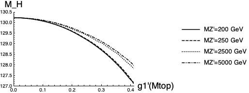
Figure 1: Higgs mass for various $g_{1}^{\prime}$ and $M_{Z^{\prime}}$, $y_{t}=0.94759$

As we can see on the plot for large $g_{1}^{\prime}$ and small $M_{Z^{\prime}}$ the Higgs mass is getting close to the experimental value. For $y_{t}=0.9539$ one even gets $m_{H}\approx 126$ GeV. If we use more precise formulas for two-loop matching Buttazzo et al. (2013) then we get that the central value $y_{t}\approx 0.94$. For this central value and for $g_{1}^{\prime}>0.3$, $m_{Z^{\prime}}<2m_{\textrm{top}}$ Higgs mass is $m_{H}=125\pm 1.5$ GeV depending on the exact parameters. On Fig. 2 we show this dependence using two-loop matched $y_{t}=0.94$ and two-loop matched $y_{t}=0.936$ with higher order QCD corrections.

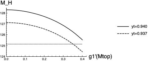
Figure 2: Higgs mass for $M_{Z^{\prime}}=200$ GeV, higher loop matching

The Model I satisfies criteria of EW vacuum stability and is of experimental and theoretical interest. The asymptotic safety predicts hat the mass of the new gauge boson should be small, which can be verified experimentally. Furthermore our argument is confirmed by the fact that for certain space of parameters the EW vacuum in the B-L extension is stable Das et al. (2017); Di Chiara et al. (2015); Delle and Marzo (2016); Z.-W.Wang et al. (2018). The effect of introducing $Z^{\prime}$ boson can be even more significant if the Higgs boson is also charged under $U_{B-L}$, see Di Chiara et al. (2015). Yet in such models $Z^{\prime}$ is highly constrained observationally with $M_{Z^{\prime}}>3$ TeV. Moreover if one relax the condition $\lambda_{3}(\mu)=0$, which is the case in more general $B-L$ models, then one immediately gets the stability of EW vacuum Grabowski et al. (2019); Latosinski et al. (2015); Lewandowski et al. (2018) and hence correct Higgs mass.
Furthermore we have checked that the $\tilde{g}$ corrections and inclusion of right handed neutrinos, botom quark and taon gives the contributions which are negligible. For instance taking into account the $y_{N}$ right handed neutrino Yukawa coupling two loop contribution Das et al. (2017) gives the difference of $10$ MeV between $y_{N}=0.0$ and $y_{N}=0.44$ situation.
In the case of Model II we perform the full two-loop analysis, with one quark $Q$ and with masses in range $m_{Q}\in(10^{5}-10^{18})$ GeV. The results are shown below on Fig. [3].

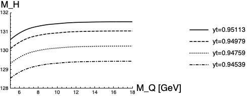
Figure 3: Optimised $\lambda(m_{\textrm{top}})$ for various $M_{Q}$(in logarithmic scale) and $y_{t}$

For Model II the new degrees of freedom influence the running of $\lambda$ much less than in Model I. The change in predicted Higgs mass at the one-loop matching is of order $1.5$ GeV downwards. There are two reasons for that. First of all addition of $Q$ changes only running of $g_{3}$, which in turn changes the running of $y_{t}$ and has only slight effect on $\lambda$. Secondly the new degrees of freedom are constrained to have mass far beyond the EW scale, while the $Z^{\prime}$ mass isn’t constrained that much both theoretically and observationally. We can conclude that inclusion of additional sterile quarks cannot drop the Higgs mass to the correct value. Yet maybe Model II combined with Model I can give the correct Higgs mass.

IV Discussion

There are a few issues which require separate discussion. First of all, to obtain the running of the considered couplings one can solve the full Wetterich equation, see for example Eichhorn and Held (2018a, b); Eichhorn (2017); Wetterich (2018). While Wetterich equation is exact, however it is very difficult (or even impossible) to be solved, because one has to take into account all of the operators which coincide with the symmetries. Moreover one has to choose the cutoff, which is arbitrary Litim. (2001); Percacci (2017). So in order to reproduce the correct perturbative results one has to take into account many higher order operators and choose the proper cutoff. As a state of the art the current FRG calculations match the usual results at the one loop level and the leading contributions to running at two-loop level Wetterich (2018) for pure gauge theories. Moreover the gravitational corrections are ambiguous due to gauge dependence, for example the prediction of top Mass ranges from $130$ to $171$ GeV only due to this effect Eichhorn and Held (2018a). For the sake of phenomenology we decided to use the loop expansion and the EFT gravitational corrections Robinson and Wilczek (2006) supplemented with the gravitational fixed point calculated with the FRG techniques Wetterich and Yamada (2019). Furthermore it seems that these two approaches give similar results (compare the fixed point of top Yukawa coupling in Shaposhnikov and Wetterich (2010) and Eichhorn and Held (2018a)).
One can also argue that $a_{i}$ Shaposhnikov and Wetterich (2010); Zanusso et al. (2010); Robinson and Wilczek (2006) are not calculated to high accuracy, making the whole calculation very sensitive to those parameters, hence not-reliable. This is indeed the case for non-Gaussian fixed point making the prediction of upper bound for top quark mass sensitive to new physics Eichhorn and Held (2018a). Yet in the case of Gaussian fixed point the existence of attractive / repelling fixed point at zero is much more vital than actual value of $a_{\lambda}$ due to the stability argument.
In our analysis we use the $\overline{MS}$ beta functions and parameters. For this scheme we cannot use the Appelquist-Carazzone theorem Appelquist and Carazzone (1975) and we rely on the effective field theory approach Weinberg (1980). In this approach one has to take into account the threshold effects Ross (1978); Hall (1981). In case of Model II the these threshold effects at two-loop precision change the prediction of Higgs mass by $5$ MeV, which is far below both experimental and theoretical accuracy. On the other hand for Model I, due to relative small mass of $Z^{\prime}$, one should fit the observables to the new set of $\overline{MS}$ couplings and then do the running, see discussion in Chankowski et al. (2006). Otherwise one can use mixed on-shell / $\overline{MS}$ scheme Chankowski et al. (2006). Both procedures are beyond the scope of this article and are left for future work. As a matter of fact this theoretical uncertainties are superseded by much bigger experimental ones in the top and Higgs mass measurements (the fact that $g_{1}^{\prime}$ is relevant parameter also contributes to this uncertainty).
Finally the $\xi_{0}$ depends not only on the matter content, but also on the gravity sector. For example in unimodular gravity Eichhorn (2013) it has slightly different value, yet the effect on Higgs mass is negligible (in naive calculations one gets $\mathcal{O}(1$ MeV)), yet it might be interesting to test it in the future. On the other hand there are other more fundamental modifications of gravity, like massive gravity de Rham (2014) or Horava gravity Horava (2009), and their fixed point structure might be completely different. Then with the right theoretical and experiment accuracy one can test quantum structure of spacetime in particle colliders far below Planck scale.

V Conclusions

In this article we have recalculated the Higgs mass in the Standard Model by taking into account the gravitational corrections and asymptotic safety requirements using the current observational bounds on $m_{\textrm{top}}$. Due to the stability bound the Higgs mass is predicted to be a higher than the experimental value.
We have investigated the two beyond SM models which improve the running of $\lambda$. In the Model I we observed that with $\lambda_{3}=0$ one gets $m_{H}\approx 125$ GeV as the lowest value, which agrees with the stability bound. However the other $Z^{\prime}$ models can give different predictions. The correct Higgs mass can also be obtained in the Conformal Standard Model Grabowski et al. (2019) where a new scalar degree of freedom is also constrained to have $m_{\phi}\approx 300$ GeV. On the other hand we have excluded the possibility that the addition of sterile quarks gives the correct $m_{H}$.
Our analysis shows that the addition of new degrees of freedom can stabilise the electroweak vacuum at the experimental value of the Higgs Boson mass. One should stress once again that whole reasoning relies on the precise measurement of the top quark mass Bezrukov and Shaposhnikov (2015) and hence the conclusions can be altered by future measurements.

References

- Meissner and Nicolai (2007) K. A. Meissner and H. Nicolai, Phys. Lett. B 648, 312 (2007), arXiv:hep-th/0612165 [hep-th] .
- Coleman and Weinberg (1973) S. Coleman and E. Weinberg, Phys. Rev. D 7, 1888 (1973).
- Gukov (2017) S. Gukov, Nucl. Phys. B919, 583 (2017), arXiv:1608.06638 [hep-th] .
- Dawid et al. (2018) S. M. Dawid, R. Gonsior, J. H. Kwapisz, K. Serafin, M. Tobolski, and S. Głazek, Phys. Lett. B777, 260 (2018), arXiv:1704.08206 [quant-ph] .
- Moroz and Schmidt (2010) S. Moroz and R. Schmidt, Annals Phys. 325, 491 (2010), arXiv:0909.3477 [hep-th] .
- t Hooft (2015) G. t Hooft, Int. J. Mod. Phys. D24, 1543001 (2015).
- t Hooft (2017) G. t Hooft, in Proceedings, 14th Marcel Grossmann Meeting on Recent Developments in Theoretical and Experimental General Relativity, Astrophysics, and Relativistic Field Theories (MG14) (In 4 Volumes): Rome, Italy, July 12-18, 2015, Vol. 1 (2017) pp. 3–12.
- Rachwał (2018) L. Rachwał, Universe 4, 125 (2018), arXiv:1808.10457 [hep-th] .
- Wetterich (2019) C. Wetterich (2019) arXiv:1901.04741 [hep-th] .
- (10) S. Weinberg, “Critical phenomena for field theorists. lectures presented at int. school of subnuclear physics,” Ettore Majorana, Erice, Sicily, Jul 23 - Aug 8 1976, Erice Subnucl.Phys.1976:1.
- Weinberg (1979) S. Weinberg, in General Relativity: An Einstein centenary survey, edited by S. W. Hawking and W. Israel (1979) pp. 790–831.
- Gastmans et al. (1978) R. Gastmans, R. Kallosh, and C. Truffin, Nucl. Phys. B133, 417 (1978).
- Christensen and Duff (1978) S. M. Christensen and M. J. Duff, Phys. Lett. 79B, 213 (1978).
- Smolin (1982) L. Smolin, Nucl. Phys. B208, 439 (1982).
- Wetterich (1993) C. Wetterich, Phys. Lett. B 301, 90 (1993), arXiv:1710.05815 [hep-th] .
- Morris (1994a) T. R. Morris, Int. J. Mod. Phys. A 9, 2411 (1994a), arXiv:hep-ph/9308265 [hep-ph] .
- Morris (1994b) T. R. Morris, Phys. Lett. B 329, 241 (1994b), arXiv:hep-ph/9403340 [hep-ph] .
- Reuter (1998) M. Reuter, Phys. Rev. D 57, 971 (1998), arXiv:hep-th/9605030 [hep-th] .
- Dou and Percacci (1998) D. Dou and R. Percacci, Class. Quant. Grav. 15, 3449 (1998), arXiv:hep-th/9707239 [hep-th] .
- Eichhorn (2018) A. Eichhorn (2018) arXiv:1810.07615 [hep-th] .
- Percacci (2017) R. Percacci, An Introduction to Covariant Quantum Gravity and Asymptotic Safety (World Scientific, 2017) https://www.worldscientific.com/doi/pdf/10.1142/10369 .
- Shaposhnikov and Wetterich (2010) M. Shaposhnikov and C. Wetterich, Phys. Lett. B 683, 196 (2010), arXiv:0912.0208 [hep-th] .
- Eichhorn and Held (2018a) A. Eichhorn and A. Held, Phys. Lett. B777, 217 (2018a), arXiv:1707.01107 [hep-th] .
- Eichhorn and Schiffer (2019) A. Eichhorn and M. Schiffer, Phys. Lett. B793, 383 (2019), arXiv:1902.06479 [hep-th] .
- Eichhorn et al. (2018a) A. Eichhorn, A. Held, and C. Wetterich, Phys. Lett. B782, 198 (2018a), arXiv:1711.02949 [hep-th] .
- Gies et al. (2017) H. Gies, R. Sondenheimer, and M. Warschinke, The European Physical Journal C 77, 743 (2017).
- Eichhorn et al. (2015) A. Eichhorn, H. Gies, J. Jaeckel, T. Plehn, M. M. Scherer, and R. Sondenheimer, JHEP 04, 022 (2015), arXiv:1501.02812 [hep-ph] .
- Loebbert and Plefka (2015) F. Loebbert and J. Plefka, Mod. Phys. Lett. A30, 1550189 (2015), arXiv:1502.03093 [hep-ph] .
- Branchina and Messina (2013) V. Branchina and E. Messina, Phys. Rev. Lett. 111, 241801 (2013), arXiv:1307.5193 [hep-ph] .
- Branchina et al. (2014) V. Branchina, E. Messina, and A. Platania, JHEP 09, 182 (2014), arXiv:1407.4112 [hep-ph] .
- Shaposhnikov (2007) M. Shaposhnikov, in Astroparticle Physics: Current Issues, 2007 (APCI07) Budapest, Hungary, June 21-23, 2007 (2007) arXiv:0708.3550 [hep-th] .
- Lewandowski et al. (2018) A. Lewandowski, K. A. Meissner, and H. Nicolai, Phys. Rev. D 97, 035024 (2018), arXiv:1710.06149 [hep-ph] .
- Chankowski et al. (2015) P. H. Chankowski, A. Lewandowski, K. A. Meissner, and H. Nicolai, Mod. Phys. Lett. A 30, 1550006 (2015), arXiv:1404.0548 [hep-ph] .
- Meissner et al. (2019) K. A. Meissner, H. Nicolai, and J. Plefka, Phys. Lett. B791, 62 (2019), arXiv:1811.05216 [hep-th] .
- Machacek and Vaughn (1985) M. E. Machacek and M. Vaughn, Nucl. Phys. B249, 70 (1985).
- Arason et al. (1992) H. Arason, D. J. Castano, B. Kesthelyi, S. Mikaelian, E. J. Piard, P. Ramond, and B. D. Wright, Phys. Rev. D46, 3945 (1992).
- Robinson and Wilczek (2006) S. P. Robinson and F. Wilczek, Phys. Rev. Lett. 96, 231601 (2006), arXiv:hep-th/0509050 [hep-th] .
- Eichhorn et al. (2018b) A. Eichhorn, Y. Hamada, J. Lumma, and M. Yamada, Phys. Rev. D 97, 086004 (2018b), arXiv:1712.00319 [hep-th] .
- Pawlowski et al. (2019) J. M. Pawlowski, M. Reichert, C. Wetterich, and M. Yamada, Phys. Rev. D99, 086010 (2019), arXiv:1811.11706 [hep-th] .
- Bennett and Nielsen (1994) D. L. Bennett and H. B. Nielsen, Int. J. Mod. Phys. A9, 5155 (1994), arXiv:hep-ph/9311321 [hep-ph] .
- Froggatt and Nielsen (1996) C. D. Froggatt and H. B. Nielsen, Phys. Lett. B368, 96 (1996), arXiv:hep-ph/9511371 [hep-ph] .
- Froggatt and Nielsen (2003) C. D. Froggatt and H. B. Nielsen, Physics. Proceedings, 31st ITEP Winter School, 6th Moscow International School, Moscow, Russia, February 18-26, 2003, Surveys High Energ. Phys. 18, 55 (2003), arXiv:hep-ph/0308144 [hep-ph] .
- Sidharth et al. (2018) B. G. Sidharth, C. R. Das, C. D. Froggatt, H. B. Nielsen, and L. Laperashvili (2018) arXiv:1801.06979 [hep-ph] .
- Buttazzo et al. (2013) D. Buttazzo, G. Degrassi, P. P. Giardino, G. F. Giudice, F. Sala, A. Salvio, and A. Strumia, JHEP 12, 089 (2013), arXiv:1307.3536 [hep-ph] .
- Bezrukov et al. (2012) F. Bezrukov, M. Yu. Kalmykov, B. A. Kniehl, and M. Shaposhnikov, Helmholtz Alliance Linear Collider Forum: Proceedings of the Workshops Hamburg, Munich, Hamburg 2010-2012, Germany, JHEP 10, 140 (2012), [,275(2012)], arXiv:1205.2893 [hep-ph] .
- Bezrukov et al. (2015) F. Bezrukov, J. Rubio, and M. Shaposhnikov, Phys. Rev. D92, 083512 (2015), arXiv:1412.3811 [hep-ph] .
- Bednyakov et al. (2015) A. V. Bednyakov, B. A. Kniehl, A. F. Pikelner, and O. L. Veretin, Phys. Rev. Lett. 115, 201802 (2015), arXiv:1507.08833 [hep-ph] .
- Tanabashi et al. (2018) M. Tanabashi et al. (Particle Data group), Phys. Rev. D 98, 030001 (2018).
- Sirlin and Zucchini (1986) A. Sirlin and R. Zucchini, Nuclear Physics B 266, 389 (1986).
- Bednyakov et al. (2017) A. V. Bednyakov, B. A. Kniehl, A. F. Pikelner, and O. L. Veretin, Nucl. Phys. B916, 463 (2017), arXiv:1612.00660 [hep-ph] .
- Dimopoulos et al. (1981) S. Dimopoulos, S. Raby, and F. Wilczek, Phys. Rev. D 24, 1681 (1981).
- Buras et al. (1978) A. Buras, J. Ellis, M. Gaillard, and D. Nanopoulos, Nuc. Phys. B 135, 66 (1978).
- Ibáñez and Ross (1981) L. Ibáñez and G. Ross, Phys. Lett. B 105, 439 (1981).
- Wetterich and Yamada (2019) C. Wetterich and M. Yamada, (2019), arXiv:1906.01721 [hep-th] .
- Patt and Wilczek (2006) B. Patt and F. Wilczek, (2006), arXiv:hep-ph/0605188 [hep-ph] .
- Shaposhnikov and Tkachev (2006) M. Shaposhnikov and I. Tkachev, Phys. Lett. B 639, 414 (2006), arXiv:hep-ph/0604236 [hep-ph] .
- Drewes (2013) M. Drewes, Int. J. Mod. Phys. E22, 1330019 (2013), arXiv:1303.6912 [hep-ph] .
- Eichhorn and Scherer (2014) A. Eichhorn and M. M. Scherer, Phys. Rev. D90, 025023 (2014), arXiv:1404.5962 [hep-ph] .
- Eichhorn et al. (2018c) A. Eichhorn, Y. Hamada, J. Lumma, and M. Yamada, Phys. Rev. D 97, 086004 (2018c), arXiv:1712.00319 [hep-th] .
- Langacker (2009) P. Langacker, Rev. Mod. Phys. 81, 1199 (2009), arXiv:0801.1345 [hep-ph] .
- Chankowski et al. (2006) P. H. Chankowski, S. Pokorski, and J. Wagner, Eur. Phys. J. C47, 187 (2006), arXiv:hep-ph/0601097 [hep-ph] .
- Basso (2011) L. Basso, Phenomenology of the minimal B-L extension of the Standard Model at the LHC, Ph.D. thesis, Southampton U. (2011), arXiv:1106.4462 [hep-ph] .
- Aaij et al. (2016) R. Aaij et al. (LHCb), JHEP 02, 104 (2016), arXiv:1512.04442 [hep-ex] .
- Aaij et al. (2017) R. Aaij et al. (LHCb), JHEP 08, 055 (2017), arXiv:1705.05802 [hep-ex] .
- Sierra et al. (2015) A. D. Sierra, F. Staub, and A. Vicente, Phys. Rev. D92, 015001 (2015), arXiv:1503.06077 [hep-ph] .
- Altmannshofer and Straub (2015) W. Altmannshofer and D. M. Straub, Eur. Phys. J. C75, 382 (2015), arXiv:1411.3161 [hep-ph] .
- Chiang et al. (2014) C.-W. Chiang, T. Nomura, and K. Yagyu, JHEP 05, 106 (2014), arXiv:1402.5579 [hep-ph] .
- Kim (1979) J. E. Kim, Phys. Rev. Lett. 43, 103 (1979).
- Shifman et al. (1980) M. A. Shifman, A. Vainshtein, and V. I. Zakharov, Nuclear Physics B 166, 493 (1980).
- Ellis and Gaillard. (1979) J. R. Ellis and M. K. Gaillard., Nucl. Phys. B150, 141 (1979).
- Peccei and Quinn (1977) R. D. Peccei and H. R. Quinn, Phys. Rev. Lett. 38, 1440 (1977).
- Das et al. (2017) A. Das, N. Okada, and N. Papapietro, Eur. Phys. J. C77, 122 (2017), arXiv:1509.01466 [hep-ph] .
- del Aguila et al. (1988) F. del Aguila, G. D. Coughlan, and M. Quiros, Nucl. Phys. B307, 633 (1988), [Erratum: Nucl. Phys.B312,751(1989)].
- Luo and Xiao (2003) M.-x. Luo and Y. Xiao, Phys. Lett. B555, 279 (2003), arXiv:hep-ph/0212152 [hep-ph] .
- Di Chiara et al. (2015) S. Di Chiara, V. Keus, and O. Lebedev, Phys. Lett. B744, 59 (2015), arXiv:1412.7036 [hep-ph] .
- Delle and Marzo (2016) C. C. R. L. Delle and C. Marzo, JHEP 02, 135 (2016), arXiv:1510.02379 [hep-ph] .
- Z.-W.Wang et al. (2018) Z.-W.Wang, F. S. S., T. Steele, and R. B. Mann, J. Phys. G45, 095002 (2018), arXiv:1511.02531 [hep-ph] .
- Grabowski et al. (2019) F. Grabowski, J. H. Kwapisz, and K. A. Meissner, Phys. Rev. D 99, 115029 (2019).
- Latosinski et al. (2015) A. Latosinski, A. Lewandowski, K. A. Meissner, and H. Nicolai, JHEP 2015, 170 (2015), arXiv:1507.01755 [hep-ph] .
- Eichhorn and Held (2018b) A. Eichhorn and A. Held, Phys. Rev. Lett. 121, 151302 (2018b), arXiv:1803.04027 [hep-th] .
- Eichhorn (2017) A. Eichhorn, in Black Holes, Gravitational Waves and Spacetime Singularities Rome, Italy, May 9-12, 2017 (2017) arXiv:1709.03696 [gr-qc] .
- Wetterich (2018) C. Wetterich, Nucl. Phys. B934, 265 (2018), arXiv:1710.02494 [hep-th] .
- Litim. (2001) D. F. Litim., Phys. Rev. D64, 105007 (2001), arXiv:hep-th/0103195 [hep-th] .
- Zanusso et al. (2010) O. Zanusso, L. Zambelli, G. P. Vacca, and R. Percacci, Phys. Lett. B 689, 90 (2010), arXiv:0904.0938 [hep-th] .
- Appelquist and Carazzone (1975) T. Appelquist and J. Carazzone, Phys. Rev. D 11, 2856 (1975).
- Weinberg (1980) S. Weinberg, Phys. Lett. 91B, 51 (1980).
- Ross (1978) D. A. Ross, Nucl. Phys. B140, 1 (1978).
- Hall (1981) L. J. Hall, Nucl. Phys. B178, 75 (1981).
- Eichhorn (2013) A. Eichhorn, Class. Quant. Grav. 30, 115016 (2013), arXiv:1301.0879 [gr-qc] .
- de Rham (2014) C. de Rham, Living Rev. Rel. 17, 7 (2014), arXiv:1401.4173 [hep-th] .
- Horava (2009) P. Horava, Phys. Rev. D79, 084008 (2009), arXiv:0901.3775 [hep-th] .
- Bezrukov and Shaposhnikov (2015) F. Bezrukov and M. Shaposhnikov, J. Exp. Theor. Phys. 120, 335 (2015), [Zh. Eksp. Teor. Fiz.147,389(2015)], arXiv:1411.1923 [hep-ph] .