Analysis of conforming, non-matching, and polygonal methods for Darcy and advection-diffusion-reaction simulations in discrete fracture networks

Abstract

The aim of this study is to compare numerical methods for the simulation of single-phase flow and transport in fractured media, described here by means of the Discrete Fracture Network (DFN) model. A Darcy problem is solved to compute the advective field, then used in a subsequent time dependent transport-diffusion-reaction problem. The numerical schemes are benchmarked in terms of flexibility in handling geometrical complexity, mass conservation and stability issues for advection dominated flow regimes. To this end, three benchmark cases have been specifically designed and are here proposed, representing some of the most critical issues encountered in DFN simulations.

1 Introduction

The movement of liquids in the underground is heavily influenced by the presence of fractures and their relative intersections [24, 37, 26]. Fractures are discontinuities (here assumed planar) along which a rock has been broken, mainly due to geological movements or to artificial stimulation [43]. In this work, we are considering only open structures, characterized by a geometrical aperture, that allow a liquid to flow through [25]. Possibilities are actual fractures, faults, and joints. We are thus excluding low permeable (closed/impervious) objects such as veins or dykes. For particular underground compositions (e.g., granite, shale, or sandstone) the rock permeability is several orders of magnitude smaller than the fracture permeability. It is a common choice and a reasonable approximation to ignore the rock matrix effect in the simulations and rely only on the fractures. The framework is the discrete fracture network model (DFN), where the aperture is not a geometrical constraint but a parameter in the bidimensional representation of the fractures by reduced models, see [42] and the forthcoming references.

The geometrical complexity of natural fracture networks may impose difficulties in the numerical simulations, due to the presence of small intersections between fractures, different intersection configurations (e.g., Y-type or L-type), small angles of intersection, and small distances between intersection lines. In the literature, three main approaches are developed to overcome these difficulties.

The first approach considers rather standard numerical scheme for the discretization of the physical equations, and relies on robust grid generation software. The coupling conditions among fractures are imposed via Lagrange multipliers on a representation of the interfaces conforming with the computational mesh on all sides. To be specific, the edges of the computational elements have to match at the intersections. This approach, commonly known as conforming discretization, may suffer, for example, when intersections lines are very close to each other, see [38, 39, 44, 45]. To partially overcome these problems, a possibility is to consider the class of virtual element methods that allows grid elements of general shapes. Two different numerical methods of this type are introduced in [8, 30, 10, 31, 12].

A second possibility is to keep the intersections explicitly represented, but relaxing the conformity of the edges. This approach, named non-conforming, requires more advanced numerical schemes based on the mortar technique. In this case, we relax the actual generation of the fracture meshes which usually gives less discrete elements than the conforming approach [7, 46]. This method may still suffer in presence of severe geometries. Also in this case the virtual element methods are an interesting option to further decrease the computational cost, see [4, 6].

A third family of schemes comprises the so-called non-matching discretizations. In terms of mesh generation, in this case the intersections do not place any constraints, as the fractures are meshed independently and the coupling conditions are imposed by an optimization procedure. A functional that measures the mismatch in the coupling conditions is minimized iteratively, where only the degrees of freedom involved in the intersections (the cut region) are considered [18, 19, 20, 11, 21]. This procedure is independent on the actual numerical schemes, might take advantage of ad-hoc strategies to enrich the solution in the cut region. Extended finite elements are a successful example, see, for example, [23, 27, 34, 35].

The present work extends and enriches the one proposed in [32] to more complex physical phenomena. The concepts previously discussed are applied to Darcy and heat transport-and-diffusion models. The Darcy velocity is computed first and then used as an advective field for the heat equation. High quality computation or reconstruction of the Darcy velocity may significantly impact the temperature distribution. Moreover, in the heat equation the transport part usually dominates the diffusion (Péclet greater than 1) and stable or stabilized schemes are needed to avoid or limit spurious oscillations that might compromise the accuracy of the solution. In the numerical tests, we are considering several numerical schemes for the comparison to cover most of the combinations discussed and try to assess their performances. The aim of this work is thus twofold: establish a set of benchmark cases and give guidance in the development of more advanced numerical schemes to solve this problem.

The paper is organized as follow. In Section 2 the Darcy and heat models are introduced and discussed, with particular focus on the coupling conditions. Section 3 is devoted to the description of the proposed numerical schemes. Three numerical examples are presented and discussed in Section 4, comparing the performances of the considered numerical schemes. Finally, in Section 5 we draw some conclusions and suggestions for future developments.

2 Mathematical model

In this section we introduce the mathematical model used to describe the hydraulic head and Darcy velocity profiles in a discrete fracture network. Once this problem is solved, the Darcy velocity is considered as advective field to simulate the transport and diffusion of heat in DFNs.

Fractures are considered as non-overlapping planar objects, which can be connected to other fractures through intersection segments, also called traces. We consider $N_{\Omega}$ fractures $\Omega_{i}\subset\mathbb{R}^{3}$ with boundary $\partial\Omega_{i}$, which compose the discrete fracture network $\Omega=\cup_{i=1}^{N_{\Omega}}\Omega_{i}$, and we denote its boundary as $\partial\Omega$ with outward unit normal $\bm{n}_{\rm ext}$, defined on each fracture plane as the unit vector normal to the fracture boundary pointing outward from the fracture polygon. To keep the presentation clear, we make a distinction between external boundaries, where we will impose data, and internal interfaces, i.e. the traces, where we will couple the mathematical models on the fractures.

Given two distinct and intersecting fractures $\Omega_{i}$ and $\Omega_{j}$, with $i\neq j$, we indicate their intersection (trace) as $\overline{\Gamma_{k}}=\overline{\Omega_{i}}\cap\overline{\Omega_{j}}$. For simplicity, we assume that a trace is formed only by two distinct fractures, however this assumption can be relaxed. A natural order of indexes can be introduced to numerate the traces $\Gamma_{k}$ from 1 to $N_{\Gamma}$, being the latter their cardinality. We consider also the function $t:\{1,\ldots,N_{\Omega}\}\times\{1,\ldots,N_{\Omega}\}\rightarrow\{1,\ldots,N_{\Gamma}\}$ such that $k=t(i,j)$ with $\overline{\Gamma_{k}}=\overline{\Omega_{i}}\cap\overline{\Omega_{j}}$. We have $t(i,j)=t(j,i)$ and its inverse $t^{-1}$ is well defined such that $(i,j)=t^{-1}(k)$ where $i<j$. We indicate with $\Gamma=\cup_{k=1}^{N_{\Gamma}}\Gamma_{k}$ the union of all the traces and by $\Gamma_{\Omega_{i}}$ the set of traces belonging to the fracture $\Omega_{i}$. Moreover, consider a fracture $\Omega_{i}$ and a trace $\Gamma_{k}$, with $k\in\Gamma_{\Omega_{i}}$. $\Gamma_{k}$ naturally subdivides $\Omega_{i}$ in two sub-regions, indicated by $\Omega_{i,+}^{k}$ and $\Omega_{i,-}^{k}$, such that $\Gamma_{k}\subset(\partial\Omega_{i,+}^{k}\cap\Omega_{i,-}^{k})$. To each of these sub-regions we associate an outward unit normal perpendicular to $\Gamma_{k}$, denoted by $\bm{n}_{i,+}$ and $\bm{n}_{i,-}$ (with $\bm{n}_{i,+}=-\bm{n}_{i,-}$) and a trace operator, respectively denoted by $\operatorname{{\rm tr}}_{i,+}^{k}$ and $\operatorname{{\rm tr}}_{i,-}^{k}$. Generic trace operators on fracture $\Omega_{i}$ are denoted by $\operatorname{{\rm tr}}_{i}$. An example of a simple DFN with the introduced nomenclature is given in Figure 1.

Figure 1: Representation of two fractures $\Omega_{i}$ and $\Omega_{j}$ intersecting in $\Gamma_{k}$.

We present the Darcy problem in strong and weak form in Subsection 2.1, to compute the hydraulic head and Darcy velocity, whereas the heat equation is introduced along with its weak formulation and functional setting in Subsection 2.2.

2.1 The Darcy model

This section is devoted to the presentation of the mathematical models used to describe the hydraulic head field $h$ and Darcy velocity $\bm{u}$ in a discrete fracture network, further details being available in [18, 19, 30, 32] and references therein. Unknowns and parameters restricted to a fracture $\Omega_{i}$ are denoted by a subscript $i$.

For clarity in the exposition, we start considering a single fracture $\Omega_{i}$. The Darcy model on $\Omega_{i}$ reads: find $(\bm{u}_{i},h_{i})$ such that

$$\begin{aligned} &\bm{u}_{i}+K_{i}\nabla h_{i}=\bm{0}\\ &\nabla\cdot\bm{u}_{i}=f_{i}\end{aligned}\quad\text{in }\Omega_{i}\setminus\Gamma$$ (1a)

Variables, data and differential operators are defined on the tangent plane of the fracture. $$K_{i} f_{i} k_{i}=\epsilon_{i}^{2}/12 \epsilon_{i}$$ is the hydraulic conductivity tensor, which is symmetric and positive definite, and is a scalar source/sink term. In our applications, following lubrication theory [2, 51, 49], we consider a scalar permeability, obtained by the cubic law: , where is the fracture aperture. Moreover, the hydraulic conductivity in (1a) is isotropic and defined as

$$K_{i}=\frac{\epsilon_{i}k_{i}\rho_{w}g}{\mu}I\,,$$

with $$\rho_{w} g \mu$$ the fluid density, the gravity acceleration, the dynamic viscosity of the fluid.

The boundary conditions on $\Omega_{i}$ are

$$\begin{aligned} &\operatorname{{\rm tr}}_{i}^{\partial}h_{i}=\overline{h}_{i}&&\text{on }\partial\Omega_{i,D}\\ &\operatorname{{\rm tr}}_{i}^{\partial}\bm{u}_{i}\cdot\bm{n}_{\rm ext}=0&&\text{on }\partial\Omega_{i,N}\end{aligned}$$ (1b)

where $\partial\Omega_{i,D}$ and $\partial\Omega_{i,N}$ are disjoint portions of the boundary of $\Omega_{i}$ such that $\overline{\partial\Omega_{i}}=\overline{\partial\Omega_{i,D}}\cup\overline{\partial\Omega_{i,N}}$, and $\operatorname{{\rm tr}}_{i}^{\partial}$ gives the trace on the boundary of $\Omega_{i}$. The data $\overline{h}_{i}$ is the given pressure head at the boundary $\partial\Omega_{i,D}$ and we model $\partial\Omega_{i,N}$ as impervious. Other boundary conditions are possible, however, in order to keep the presentation as simple as possible and coherent with the examples proposed in Section 4, we consider only these, being the generalization to other boundary conditions straightforward. We assume, for a single fracture, that $\partial\Omega_{i,D}$ is not empty; in presence of intersecting fractures, instead, we can have $\partial\Omega_{i,D}=\emptyset$ for all the fractures but one. Equations (1a) and (1b) are well studied in the literature, refer to the aforementioned references.

Let us now consider two distinct fractures $\Omega_{i}$ and $\Omega_{j}$ forming an intersection $\Gamma_{k}$. On both fractures we apply Equations (1a) and (1b) and we assume continuous coupling conditions for the hydraulic head and the normal component of the Darcy velocity at the trace. The coupling conditions between two fractures $\Omega_{i}$ and $\Omega_{j}$ such that $t(i,j)=k$, read

$$\begin{aligned} &\sum_{l\in\{i,j\}}\operatorname{{\rm tr}}_{l,+}^{k}\bm{u}_{l}\cdot\bm{n}_{l,+}+\operatorname{{\rm tr}}_{l,-}^{k}\bm{u}_{l}\cdot\bm{n}_{l,-}=0\\ &\operatorname{{\rm tr}}_{i,+}^{k}h_{i}=\operatorname{{\rm tr}}_{i,-}^{k}h_{i}=\operatorname{{\rm tr}}_{j,+}^{k}h_{j}=\operatorname{{\rm tr}}_{j,-}^{k}h_{j}\end{aligned}\quad\text{on $\Gamma_{k}$}\,.$$ (1c)

The case of multiple fractures follows immediately from our assumptions. The Darcy equation can be formalised in the following problem.

Problem 1 (Darcy equation on a DFN - mixed formulation).

Given the set of fractures $\Omega$ and traces $\Gamma$, find $(\bm{u},h)$ such that (1a)-(1b)-(1c) are satisfied.

The weak formulation of Problem 1 requires the introduction of the functional spaces on each $\Omega_{i}$, namely

$${V}_{i}=H_{\nabla\cdot}(\Omega_{i})=\left\{\bm{v}\in\left[L^{2}(\Omega_{i})\right]^{2}:\,\nabla\cdot\bm{v}\in L^{2}(\Omega_{i})\right\}\quad\text{and}\quad Q_{i}=L^{2}(\Omega_{i})\,,$$

equipped with the natural norms that make them complete. The spaces for the global network are

$$\begin{split}V&=\left\{\bm{v}\colon\bm{v}_{i}\in V_{i}\,,\,\operatorname{{\rm tr}}_{i}^{\partial}\bm{v}_{i}\cdot\bm{n}_{\rm ext}=0\text{ on $\partial\Omega_{i,N}$}\quad\forall i\,,\vphantom{\sum_{l\in\{i,j\}}}\right.\\ &\quad\left.\sum_{l\in\{i,j\}}\operatorname{{\rm tr}}_{l,+}^{k}\bm{u}_{l}\cdot\bm{n}_{l,+}+\operatorname{{\rm tr}}_{l,-}^{k}\bm{u}_{l}\cdot\bm{n}_{l,-}=0\quad\forall k\,,\,t^{-1}(k)=(i,j)\right\}\,,\end{split}$$

and $Q=\bigoplus_{i}Q_{i}$, both endowed with their natural norms. The following linear forms are then introduced: $a_{i}:V_{i}\times V_{i}\rightarrow\mathbb{R}$, $b_{i}:V_{i}\times Q_{i}\rightarrow\mathbb{R}$, $G_{i}:\left(H^{\frac{1}{2}}(\partial\Omega_{i,D})\right)^{\prime}\rightarrow\mathbb{R}$ and $F_{i}:Q_{i}\rightarrow\mathbb{R}$ such that, $\forall\bm{u},\bm{v}\in V_{i}$ and $\forall q\in Q_{i}$

$$a_{i}(\bm{u},\bm{v}) =\left(K_{i}^{-\frac{1}{2}}\bm{u},K_{i}^{-\frac{1}{2}}\bm{v}\right)_{\Omega_{i}}\,, b_{i}(\bm{u},q) =-(\nabla\cdot\bm{u},q)_{\Omega_{i}}\,,$$

$$G_{i}(\bm{v}) =-\langle\overline{h}_{i},\operatorname{{\rm tr}}_{i}\bm{v}\cdot\bm{n}\rangle_{\partial\Omega_{i,D}}\,, F_{i}(q) =-(f,q)_{\Omega_{i}}\,.$$

We also require that $f\in Q_{i}$, $\overline{h}_{i}\in H^{\frac{1}{2}}(\partial\Omega_{i,D})$, and $K_{i}\in L^{\infty}(\Omega_{i})$. The less standard functional spaces associated with $G_{i}$ are due to the low regularity of a $H_{\nabla\cdot}$-function at a boundary, as well as the duality pairing used instead of a scalar product. The global forms $a:V\times V\rightarrow\mathbb{R}$, $b:V\times Q\rightarrow\mathbb{R}$, $G:H^{*}\rightarrow\mathbb{R}$, and $F:Q\rightarrow\mathbb{R}$ are the sums of the respective local ones, where we denoted by $H^{*}=\bigoplus_{i}\left(H^{\frac{1}{2}}(\partial\Omega_{i,D})\right)^{\prime}$, the space associated to the boundary term.

Problem 2 (Darcy equation on a DFN - mixed weak formulation).

The weak formulation of Problem 1 is: find $(\bm{u},h)\in V\times Q$ such that

$$a(\bm{u},\bm{v})+b(\bm{v},h)=G(\bm{v}) \forall\bm{v}\in V$$

$$b(\bm{u},q)=F(q) \forall q\in Q$$

Some numerical formulations require the problem written in term of pressure head alone, thus we consider also the primal formulation of Problem 1. Given a fracture $\Omega_{i}$ the model is: find $h_{i}$ such that

$$\begin{aligned} &-\nabla\cdot\left(K_{i}\nabla h_{i}\right)=f_{i}&&\text{in }\Omega_{i}\setminus\Gamma\\ &\operatorname{{\rm tr}}_{i}h_{i}=\overline{h}_{i}&&\text{on }\partial\Omega_{i,D}\\ &\operatorname{{\rm tr}}_{i}K_{i}\nabla{h}_{i}\cdot\bm{n}_{\rm ext}=0&&\text{on }\partial\Omega_{i,N}\end{aligned}$$ (2a)

Given a second distinct fracture $$\Omega_{j} \Omega_{i} \Gamma_{k}$$ which intersects in , the following coupling conditions are added:

$$\begin{aligned} &\sum_{l\in\{i,j\}}\operatorname{{\rm tr}}_{l,+}K_{l}\nabla h_{l}\cdot\bm{n}_{l,+}+\operatorname{{\rm tr}}_{l,-}K_{l}\nabla h_{l}\cdot\bm{n}_{l,-}=0\\ &\operatorname{{\rm tr}}_{i,+}^{k}h_{i}=\operatorname{{\rm tr}}_{i,-}^{k}h_{i}=\operatorname{{\rm tr}}_{j,+}^{k}h_{j}=\operatorname{{\rm tr}}_{j,-}^{k}h_{j}\end{aligned}\quad\text{on }\Gamma_{k}.$$ (2b)

Once the pressure head is computed, the Darcy velocity is given by the first equation of (1a). We can formalize also the primal formulation of the Darcy equation in the following problem.

Problem 3 (Darcy equation on a DFN - primal formulation).

Given the set of fractures $\Omega$ and traces $\Gamma$, find $h$ such that (2a)-(2b) are satisfied $\forall i,k$.

In this case, the weak formulation is simpler than the previous one. To keep the notation standard and since we are introducing a separate formulation of the Darcy problem, in the following we commit abuses in notation. We introduce the functional spaces

$$V_{i}=\{v\in H^{1}(\Omega_{i}):\,\operatorname{{\rm tr}}_{i}^{\partial}v=\overline{h}_{i}\text{ on }\partial\Omega_{i,D}\}\,,$$

and $V_{i,0}$ in the special case of homogeneous head condition. The linear forms now read: $a_{i}:V_{i}\times V_{i,0}\rightarrow\mathbb{R}$ and $F:V_{i,0}\rightarrow\mathbb{R}$ such that, $\forall v\in V_{i,0}$,

$$a_{i}(h,v)=(K_{i}^{\frac{1}{2}}\nabla h,K_{i}^{\frac{1}{2}}\nabla v)_{\Omega_{i}}\quad\text{and}\quad F_{i}(v)=(f,v)_{\Omega_{i}}\,.$$

In this case, we ask $f\in\left(V_{i,0}\right)^{\prime}$, $\overline{h}_{i}\in H^{\frac{1}{2}}(\partial\Omega_{i,D})$, and $K_{i}\in L^{\infty}(\Omega_{i})$. The functional spaces on the whole network are

$$\begin{split}V=\left\{v\colon v_{i}\in V_{i}\quad\forall i\,,\quad\operatorname{{\rm tr}}_{i,+}^{k}v_{i}=\operatorname{{\rm tr}}_{i,-}^{k}v_{i}=\operatorname{{\rm tr}}_{j,+}^{k}v_{j}=\operatorname{{\rm tr}}_{j,-}^{k}v_{j}\quad\right.&\\ \quad\left.\forall k\,,\,t^{-1}(k)=(i,j)\right\}&\,,\end{split}$$

$$\begin{split}V_{0}=\left\{v\colon v_{i}\in V_{i,0}\quad\forall i\,,\quad\operatorname{{\rm tr}}_{i,+}^{k}v_{i}=\operatorname{{\rm tr}}_{i,-}^{k}v_{i}=\operatorname{{\rm tr}}_{j,+}^{k}v_{j}=\operatorname{{\rm tr}}_{j,-}^{k}v_{j}\quad\right.&\\ \quad\left.\forall k\,,\,t^{-1}(k)=(i,j)\right\}&\,,\end{split}$$

with their natural norms. The global forms $a:V\times V_{0}\rightarrow\mathbb{R}$ and $F:V_{0}\rightarrow\mathbb{R}$ are the sums of the respective local ones.

Problem 4 (Darcy equation on a DFN - primal weak formulation).

The weak formulation of Problem 3 is: find $h\in V$ such that

$$a(h,v)=F(v)\qquad\forall v\in V_{0}\,.$$

We note that to obtain symmetric forms in Problem 4 a lifting technique of the Dirichlet datum can be considered.

2.2 The heat equation

In this part, we present the heat equation on the DFN. Once Problem 1 is solved, the Darcy velocity can be used as advective field in the transport problem. We denote the temperature in a DFN as $\theta$, and its restriction to fracture $\Omega_{i}$ as $\theta_{i}$. The heat equation on $\Omega_{i}$ reads: given $\bm{u}_{i}$ find $\theta_{i}$ such that

$$\zeta_{i}\partial_{t}\theta_{i}+\nabla\cdot(\bm{u}_{i}\theta_{i}-D_{i}\nabla\theta_{i})+\iota_{i}(\theta_{i}-\hat{\theta}_{i})=0\quad\text{in }\Omega_{i}\setminus\Gamma\times(0,T]\,,$$ (3a)

where $$T\in\mathbb{R}$$ is the end time of the simulation. Also in this case, the variables, data, and differential operators are defined on the tangent plane of the fracture. The relations to compute the physical parameters are [2, 51, 49]:

$$\zeta_{i} =\frac{\epsilon_{i}c_{e,i}}{\rho_{w}c_{w}}\,, D_{i} =\frac{\epsilon_{i}\lambda_{e,i}}{\rho_{w}c_{w}}\,, \iota_{i} =\frac{\gamma_{e,i}}{\rho_{w}c_{w}}\,,$$

where $$\epsilon_{i} \rho_{w} c_{w} c_{e,i}=\phi_{i}\rho_{w}c_{w}+(1-\phi_{i})\rho_{m}c_{m} \phi_{i} \rho_{m} c_{m} \lambda_{e,i}=\lambda_{w}^{\phi_{i}}\lambda_{m}^{1-\phi_{i}} \gamma_{e,i} \hat{\theta}_{i} \phi_{i}=1 \phi_{i}<1$$ is the fracture aperture, the fluid density, the fluid specific thermal capacity, the fracture effective thermal capacity, the fracture porosity, the density of the rock matrix, the specific thermal capacity of the rock matrix, the effective thermal conductivity, the effective heat transfer coefficient between fluid and rock, and, finally, is the temperature of the rock matrix, acting as external heat source/sink. When the fracture is completely open and no sediments are present, whereas values of indicate that fracture is partially filled with crystals/rocks. Equation (3a) is in conservative form, being the total flux the conserved quantity.

For the sake of brevity and clarity of explanation we do not present boundary conditions in the most general context, but conforming to the numerical tests of Section 4; generalization is however again straightforward. Recalling that $\partial\Omega_{i,D}$ is the Dirichlet portion of the boundary of fracture $\Omega_{i}$ for the Darcy problem in Section 2.1, let us split $\partial\Omega_{i,D}$ into two parts, namely $\partial\Omega_{i,D}^{\rm inflow}$ and $\partial\Omega_{i,D}^{\rm outflow}$. Thus, according to the computed Darcy velocity $\bm{u}_{i}$, on each fracture $\Omega_{i}$, the inflow boundary $\partial\Omega_{i,D}^{\rm inflow}$ is the portion of $\partial\Omega_{i,D}$ where $\bm{u}_{i}\cdot\bm{n}_{\rm ext}<0$ and conversely the outflow boundary is the portion of $\partial\Omega_{i,D}$ where $\bm{u}_{i}\cdot\bm{n}_{\rm ext}>0$, thus linking the nature of the boundary to the solution of the Darcy problem. Please note that $\partial\Omega_{i,D}^{\rm inflow}$ and $\partial\Omega_{i,D}^{\rm outflow}$ might be both empty for most of the fractures. Then boundary conditions on fracture $\Omega_{i}$ are:

$$\begin{aligned} &\operatorname{{\rm tr}}_{i}\theta_{i}=\overline{\theta}_{i}&&\text{on }\partial\Omega_{i,D}^{\rm inflow}\times(0,T]\,,\\ &\operatorname{{\rm tr}}_{i}D_{i}\nabla\theta_{i}\cdot\bm{n}_{\rm ext}=0&&\text{on }\partial\Omega_{i,D}^{\rm outflow}\times(0,T]\,,\\ &\operatorname{{\rm tr}}_{i}D_{i}\nabla\theta_{i}\cdot\bm{n}_{\rm ext}=0&&\text{on }\partial\Omega_{i,N}\times(0,T]\,.\end{aligned}$$ (3b)

By (1b), on the portion $\partial\Omega_{i,N}$ both the diffusive and advective terms are zero for $\theta_{i}$, so $\partial\Omega_{i,N}$ represents an impervious boundary also for the heat equation. Finally, the initial condition on $\Omega_{i}$ is given by

$$\theta_{i}=\overline{\overline{\theta_{i}}}\quad\text{in }\Omega_{i}\setminus\Gamma\times\{0\}.$$ (3c)

We consider now two distinct fractures $\Omega_{i}$ and $\Omega_{j}$ with an intersection $\Gamma_{k}$. On $\Omega_{i}$ the temperature $\theta_{i}$ fulfils (3a), (3b), and (3c). The same for $\theta_{j}$ in the fracture $\Omega_{j}$. The coupling conditions on $\Gamma_{k}\times(0,T]$ are

$$\begin{split}&\sum_{l\in\{i,j\}}\!\!\operatorname{{\rm tr}}_{l,+}(\bm{u}_{l}\theta_{l}-D_{l}\nabla\theta_{l})\cdot\bm{n}_{l,+}+\!\operatorname{{\rm tr}}_{l,-}(\bm{u}_{l}\theta_{l}-D_{l}\nabla\theta_{l})\cdot\bm{n}_{l,-}\!=\!0\,,\\ &\operatorname{{\rm tr}}_{i,+}\theta_{i}=\operatorname{{\rm tr}}_{i,-}\theta_{i}=\operatorname{{\rm tr}}_{j,+}\theta_{j}=\operatorname{{\rm tr}}_{j,-}\theta_{j}\,.\end{split}$$ (3d)

Also in this case, in presence of multiple fractures the generalization of the model is immediate. The heat equation can be formalized in the following problem.

Problem 5 (Heat equation on a DFN).

Given the set of fractures $\Omega$ and traces $\Gamma$ and the Darcy velocity $\bm{u}$, find $\theta$ such that (3a)-(3b)-(3c)-(3d) are satisfied.

To derive the weak formulation of Problem 5 we need to introduce the Bochner space

$$W_{i}^{0}=L^{2}\left(0,T;\left\{v\in H^{1}(\Omega_{i}):\,\operatorname{{\rm tr}}_{i}v\,(t)={\overline{\theta_{i}}}\,(t)\text{ on }\partial\Omega_{i,D}^{\rm inflow}\,\,\,\forall t\in(0,T]\right\}\right),$$

while for the test functions we define

$$W_{i}^{1}=H^{1}\left(0,T;\left\{v\in H^{1}(\Omega_{i}):\,\operatorname{{\rm tr}}_{i}v\,(t)=0\text{ on }\partial\Omega_{i,D}^{\rm inflow}\,\,\,\forall t\in(0,T]\right\}\right)\,.$$

We need to introduce space-time forms associated to each fracture, in particular we have: $m_{i}$, $d_{i}$, $g_{i}$, $r_{i}$ which are defined on $W_{i}^{0}\times W_{i}^{1}\rightarrow\mathbb{R}$, and $S_{i}:W_{i}^{1}\rightarrow\mathbb{R}$ such that

$$m_{i}(\theta,v)=-\int_{0}^{T}(\theta,\partial_{t}\zeta_{i}v)_{\Omega_{i}}\qquad d_{i}(\theta,v)=\int_{0}^{T}(D_{i}^{\frac{1}{2}}\nabla\theta,D_{i}^{\frac{1}{2}}\nabla v)_{\Omega_{i}}$$

$$g_{i}(\theta,v)=\int_{0}^{T}(\nabla\cdot(\bm{u}_{i}\theta),v)_{\Omega_{i}}\quad r_{i}(\theta,v)=\int_{0}^{T}(\iota_{i}\theta,v)_{\Omega_{i}}$$

$$S_{i}(v)=\int_{0}^{T}(\iota_{i}\hat{\theta}_{i},v)_{\Omega_{i}}+(\overline{\overline{\theta_{i}}},v(0))_{\Omega_{i}}$$

The global functional spaces are

$$\begin{split}W^{0}=\left\{v\colon v_{i}\in W_{i}^{0}\quad\forall i\,,\,\operatorname{{\rm tr}}_{i,+}^{k}v_{i}(t)=\operatorname{{\rm tr}}_{i,-}^{k}v_{i}(t)=\operatorname{{\rm tr}}_{j,+}^{k}v_{j}(t)=\operatorname{{\rm tr}}_{j,-}^{k}v_{j}(t)\quad\right.&\\ \quad\left.\forall t\in(0,T]\,,\,\forall k\,,\,t^{-1}(k)=(i,j)\right\}&\,,\end{split}$$

$$\begin{split}W^{1}=\left\{v\colon v_{i}\in W_{i}^{1}\quad\forall i\,,\,\operatorname{{\rm tr}}_{i,+}^{k}v_{i}(t)=\operatorname{{\rm tr}}_{i,-}^{k}v_{i}(t)=\operatorname{{\rm tr}}_{j,+}^{k}v_{j}(t)=\operatorname{{\rm tr}}_{j,-}^{k}v_{j}(t)\quad\right.&\\ \quad\left.\forall t\in(0,T]\,,\,\forall k\,,\,t^{-1}(k)=(i,j)\right\}&\,,\end{split}$$

and the global bilinear forms $m$, $d$, $g$, $r$ and $S$ are the sum over all fractures of the local ones. We finally have the weak formulation of the problem.

Problem 6 (Heat equation on a DFN - weak formulation).

The weak formulation of Problem 5 is: find $\theta\in W^{0}$ such that

$$m(\theta,v)+d(\theta,v)+g(\theta,v)+r(\theta,v)=S(v)\qquad\forall v\in W^{1}\,.$$

Also in this case to obtain a symmetric problem we can use a lifting technique of the Dirichlet datum.

3 Numerical discretization

In this section, we present various discretization strategies, both well established, both unconventional, that can be used to solve the models described in Section 2. These strategies have similarities and differences that can be used to categorize them. A first point concerns the computational mesh and, in particular, how the meshing is performed at fracture intersections: it is possible to have a matching or non-matching grids. In the former case fracture grids are conforming to the intersections among fractures, while in the latter, grid elements arbitrarily cross intersections. A second issue is related to mass conservation: in computing the Darcy velocity, some schemes are locally mass conservative and some other are only globally conservative, and this property may impact the subsequent solution of the heat problem. Also, some numerical schemes are characterized by high numerical diffusivity which might impact the solution but also avoids nonphysical spurious oscillations in advection dominated flow regimes, whereas other schemes need to adopt stabilitazion techniques.

Six different approaches are considered in the present work, given as the combination of a numerical scheme for the computation of the Darcy velocity and a numerical scheme for the spatial semi-discretization of the subsequent non-stationary advection-diffusion-reaction problem (shortly denoted as Heat equation). The implicit Euler method is used, instead, in all cases, for time evolution. The approaches are listed in Table 1. The scheme tagged tpfaup is given by the combination of the Two Point Flux Approximation (tpfa) method for the Darcy problem and the TPFA with upwinding for the advection term (tpfa+upwind) for the Heat equation. Scheme mfemup uses, instead mixed finite elements (mfem) for the Darcy equation and again tpfa+upwind for the Heat equation. The method mvemup, uses instead the Virtual Element Method in mixed formulation (mvem) for the Darcy problem, on matching polygonal meshes. These schemes are implemented in PorePy, a simulation tool written in Python for fractured and deformable porous media, see [41, 40]. PorePy is freely available on GitHub along with the numerical tests proposed in Section 4. The method labeled mfemsupg is based on mixed standard finite elements for the numerical resolution of the Darcy problem and on standard finite elements (fem) with Streamline Upwind Petrov-Galerkin (supg) stabilization [28] for the Heat equation. Finally methods femsupg and xfemsupg use a non-conventional optimization based approach for the Darcy equation and, with supg stabilization also for the Heat equation. The optimization approach can adopt different baseline discretization methods: here we consider the variants using standard finite elements (opt-fem) and extended finite elements (opt-xfem). Methods mfemsupg femsupg and xfemsupg are implemented in C++ and Matlab^®.

The forthcoming parts describe in more details the previous approaches, grouping them according to the coupling at the traces: matching coupling at traces in Subsection 3.1 and non-matching coupling in Subsection 3.2.

Tag	Darcy eq.	Heat eq.	Grid
tpfaup	tpfa	tpfa + upwind	Matching triangles
mfemup	mfem	tpfa + upwind	Matching triangles
mvemup	mvem	tpfa + upwind	Matching polygons
mfemsupg	mfem	fem + supg	Matching triangles
femsupg	opt-fem	opt-fem + supg	Non-match. triangles
xfemsupg	opt-xfem	opt-xfem + supg	Non-match. triangles

Table 1: List of numerical schemes proposed to solve the Darcy and heat problems, with the type of meshes used.

3.1 Matching discretization at traces

Here advantages and drawbacks of a conforming discretization at the traces are discussed. As mentioned before in a conforming grid, the meshes of both the intersecting fractures match the trace with their geometry. The trace is thus entirely covered by contiguous cell edges of the two fractures, see Figure 2(a)-2(b) as an example. This approach has the clear advantage of an easy applicability to most of the existing and well established numerical methods (finite volumes, finite elements). However, in the case of complex geometries the computational cost might increase and become a severe constraint in complex fracture networks.

(a) matching triangles

(b) matching polygons obtained by coarsening

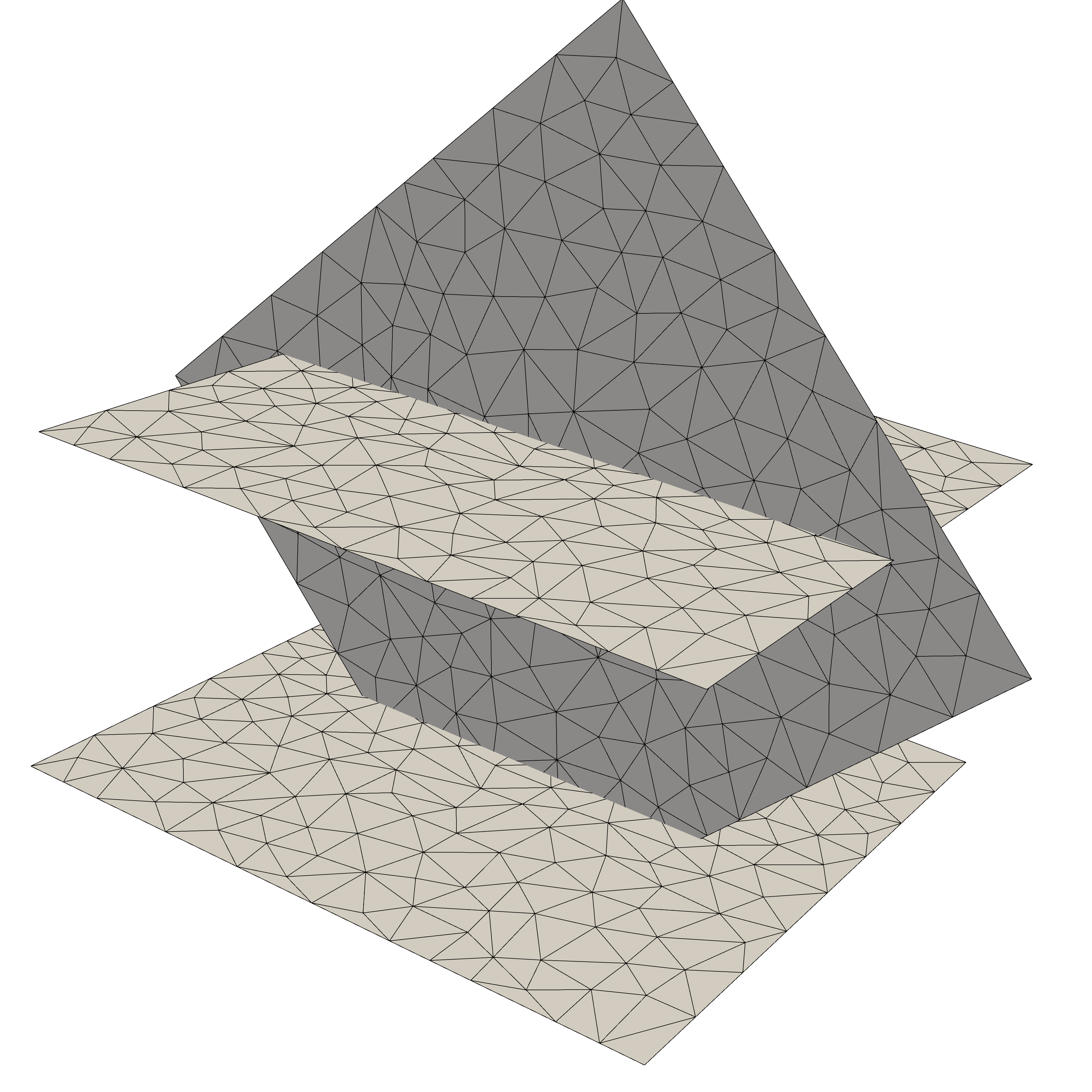
(c) non-matching triangles

Figure 2: Examples of matching meshes.

To solve the Darcy problem, we rely on different classes of numerical schemes: finite volumes, finite elements in primal and mixed formulation, and virtual elements in mixed formulation. For the finite volume class, we choose the two-point flux approximation tpfa on simplicial grids, applied to Problem 4, see [1] for details. This scheme is well known in the industry field and widely used for its velocity in assembling the discrete problem and for having a narrow matrix stencil. The scheme is locally conservative and robust with respect to strong variations of the hydraulic conductivity coefficient, however it is consistent only for $K$-orthogonal grids. Regarding the class of finite elements, we consider mixed finite elements with the pair of spaces $\mathbb{RT}_{0}-\mathbb{P}_{0}$ for the Darcy velocity and piecewise constants for the hydraulic head, denoted by mfem, defined on a simplicial grid, for further references see [47, 48]. It is well known that $\mathbb{RT}_{0}-\mathbb{P}_{0}$ is locally conservative and more robust than primal $\mathbb{P}_{1}$ finite elements with respect to strong variations on the hydraulic conductivity coefficient. On the other hand, it gives a larger linear system, with a saddle-point structure. The mfem scheme solves the Darcy problem in the form presented in Problem 2. In some particular scenarios the regularity requirements on meshes formed by triangles are too restrictive and schemes able to handle generally shaped cells are more suitable. In these cases we rely on the new class of virtual element methods, which are variational methods where the basis functions of the discrete spaces are not prescribed a-priori, and are defined implicitly on general star-shaped elements as solutions of suitable local PDEs. See the seminal works [3, 22, 5, 6] and those related to DFN [8, 7, 9, 10, 30]. In our analysis we consider only the lowest order mixed (mvem) formulation, which can be viewed as a generalization $\mathbb{RT}_{0}-\mathbb{P}_{0}$ mixed finite elements on generally shaped cells, solving Problem 2. Virtual element methods share many properties with their finite element counterpart: indeed, mvem are locally conservative, robust with respect to the hydraulic conductivity variation and have the same grid stencil of the $\mathbb{RT}_{0}-\mathbb{P}_{0}$. Here we use mvem on polygonal grids, obtained by coarsening a mesh originally made of triangular elements in order to reduce the number of cells required in the simulation for complex geometries, as described in [30, 29].

To solve the heat equation (Problem 6), we use a tpfa scheme for the diffusive term and a weighted upwind scheme for the advective term. The advantage of this choice is that we obtain a stable scheme which respects the maximum and minimum principle, without oscillation due to high grid-Péclet numbers. However, for some applications the obtained scheme might be too diffusive. Finally, we consider also standard $\mathbb{P}_{1}$ finite elements, with a supg stabilized discrete variational formulation, which is a globally conservative numerical scheme.

Since in all the above cases we have matching meshes, and thus the degrees of freedom on the trace of one fracture correspond to the degrees of freedom of the intersecting one, coupling conditions can be imposed strongly.

Methods tpfaup, mfemup and mfemsupg are considered here standard reference approaches of different discretization strategies (finite volume and finite element based), and are used to benchmark the behavior of the other less conventional approaches, based e.g. on polygonal or non-matching discretizations.

3.2 Non-matching discretization at traces

When dealing with huge networks, the generation of conforming meshes may require a large computational cost. Then, it is worth considering a class of methods that do not require any kind of conformity of the fracture meshes to traces, see, for example, Figure 2(c).

In [16, 17, 18, 19, 13, 14] a PDE-constrained optimization approach is proposed, based on non-conforming meshes, that can be applied both to Problem 4 and Problem 6. In this framework, the problem is rewritten as a minimization problem for a functional measuring the error in fulfilling matching conditions, constrained by local PDEs on each fracture. This approach provides not only a numerical approximation of the solution but also a directly computed approximation of the flux exchanged at traces, which is of interest for many applications. The discretization can be based on different methods: standard $\mathbb{P}_{1}$ finite elements are the simplest choice, and the resulting scheme is denoted as opt-fem. However, as mesh elements arbitrarily cross the traces, the jump of the co-normal derivative of the solution at fracture intersections, still directly computed by the method, can not be correctly represented by non conforming $\mathbb{P}_{1}$ finite elements. Thus the use of local extended finite elements is also considered, being at the basis of the method denoted opt-xfem. When used for advection dominated flow regimes, the supg-stabilized versions of the method are used (femsupg, xfemsupg).

The resulting numerical schemes inherit the mass-conservation properties of the local discrete formulations, thus they are globally but not locally conservative. A huge advantage of this method is that the matrices resulting from the local discrete problems can be computed in parallel, and also the solution can be computed strongly relying on parallel computing. In [20] a MPI-based parallel algorithm is proposed for assembling and solving the discrete problem using the conjugate gradient method on huge networks of fractures, whereas in [15] an implementation suitable for GPGPUs is presented.

4 Examples

In this section, we present three test cases with the aim of validating and comparing the previously introduced models. Extending the work proposed in [32], here we analyse the various approaches for time dependent problems of advection-diffusion-reaction, where the advection velocity is computed by means of the same approach solving a diffusion problem. The key aspects of the various schemes will be highlighted and investigated, along with the impact of the lack of conservation of fluxes, both locally and through a trace, that characterizes some of the proposed approaches. For the considered test cases, both local and global quantities will be computed at different time steps, and used to assess and compare the behaviour of the various approaches, such as i) the integral mean in space of the temperature on a fracture $\Omega$, denoted as $\langle{\theta}\rangle_{\Omega}$; ii) the total flux mismatch on a trace, $\delta\Phi_{\Gamma}$ defined as the integral of the sum of the net total fluxes $\Phi_{\Gamma,i}$ and $\Phi_{\Gamma,j}$ entering or leaving the two fractures $\Omega_{i}$ and $\Omega_{j}$ meeting at trace $\Gamma$, respectively, i.e. $\delta\Phi=|{\Phi_{\Gamma,i}+\Phi_{\Gamma,j}}|$,

$$\Phi_{\Gamma,i}=-\int_{\Gamma}\left(\mathop{\left[\!\!\left[\operatorname{{\rm tr}}_{i}D_{i}\nabla\theta_{i}\cdot\bm{n}_{i\Gamma}\right]\!\!\right]_{\Gamma}}\nolimits+\mathop{\left[\!\!\left[\operatorname{{\rm tr}}_{i}\theta_{i}\operatorname{{\rm tr}}_{i}\bm{u_{i}}\cdot\bm{n}_{i\Gamma}\right]\!\!\right]_{\Gamma}}\nolimits\right)$$

with $\bm{n}_{i\Gamma}$ the unit normal vectors to $\Gamma$, with fixed orientation on $\Omega_{i}$; and iii) the averaged $\theta$ on the outflow boundary, $\partial\Omega^{\mathrm{outflow}}_{D}$, denoted as

$$\langle{\theta}\rangle_{\mathrm{outflow}}:=\dfrac{1}{|{\partial\Omega^{\mathrm{outflow}}_{D}}|}\int_{\partial\Omega^{\mathrm{outflow}}_{D}}\operatorname{{\rm tr}}\theta.$$

The considered test cases are designed in order to challenge the proposed approaches with complex geometries and/or realistic models. In Subsection 4.1 we consider the effect of vanishing trace from a simple network, by a sequence of simulations. In the second example presented in Subsection 4.2 a synthetic small network of $10$ fractures is considered, to analyse the behaviour of the methods on a more general, yet simple configuration. We finally conclude with a realistic example in Subsection 4.3, where a network of 89 fractures is generated from an extrusion of an interpreted natural outcrop and physically sound values for the various parameters are used.

With the purpose of establishing a standard reference for the analysis of numerical schemes for flow in fractures, test cases in Subsections 4.1 and 4.3 are borrowed from [32] and adapted to the present context, all the geometrical data being available in [33].

4.1 Vanishing trace between intersecting fractures

As a first test case, named Test Case 1, the same setting of the problem proposed in the example of [32, Subsection 4.3.1] is considered. In the reference, the Darcy problem was tackled, whereas here a non-stationary advection-diffusion problem for the passive scalar $\theta$ is solved.

In this test case the same problem is solved on different geometries. Let us consider a network composed of three fractures, named $\Omega_{l}$, $\Omega_{r}$, and $\Omega_{c}$, as shown in Figure 3. Fracture $\Omega_{l}$ has a fixed position, whereas fractures $\Omega_{r}$, and $\Omega_{c}$ are displaced, for each different geometry of a same distance along the $z$-direction, such that the length of the intersection line between fractures $\Omega_{l}$ and $\Omega_{r}$, denoted as $\Gamma_{0}$, progressively reduces from the configuration shown in Figure 5, being instead fixed the intersection between $\Omega_{r}$, and $\Omega_{c}$, denoted as $\Gamma_{1}$. In such a way 21 different configurations are obtained, with the length of the vanishing trace $\Gamma_{0}$ ranging from $0.6$ at configuration $C0$, as shown in Figure 3, to $0.01$, at configuration $C20$. The geometries corresponding to configurations $C0$, $C10$ and $C20$ are shown in Figure 5. For each configuration, the Darcy problem, formulated as in 2 or 4, depending on the method, is first solved in order to compute the Darcy velocity $\bm{u}$, with a null source term. A unitary hydraulic conductivity $K$ is used for all the fractures and pressure head boundary conditions are prescribed on the bottom part of $\partial\Omega_{l}$ (inflow) and $\partial\Omega_{r}$ (outflow) equal to $1$ and $0$, respectively (see Figure 3). On the other portions of the boundary a no-flux boundary condition is imposed. Subsequently, an advection-diffusion problem is solved, obtained from Problem 6 setting the reaction operator $r(\cdot,\cdot)\equiv 0$, and with null source. We assume a unitary coefficient $\zeta$, a diffusion coefficient $D$ equal to $10^{-4}$ and a constant in time unitary Dirichlet boundary condition on the inflow part of the domain boundary, whereas homogeneous Neumann boundary condition are set on the rest of the boundary.

Figure 3: Geometry of Test Case 1. The inflow and outflow portions of the boundary are represented by red and blue lines, respectively.

The meshes used for the space discretization are different for conforming-triangular, conforming-polygonal and non-matching strategies, as discussed above. The mesh for the conforming schemes are generated using the Gmsh [36] library, and two different mesh parameters are used, corresponding to about $10^{3}$ and $10^{4}$ elements for the configuration $C0$. Clearly, as the length of trace $\Gamma_{0}$ progressively reduces from configuration $C0$ to $C20$, the mesh generation tool tends to increase the number of elements in order to meet the conformity requirement without compromising mesh quality. This process inevitably leads to a large increment of the number of elements from configuration $C0$ to $C20$, for each of the three initial refinement levels. The mesh for the non-matching schemes is obtained through the Triangle [50] software, using two mesh parameters, again corresponding to about $10^{3}$, and $10^{4}$ elements. In this case, instead, since the mesh is independent from the traces, the number of elements is practically unaffected by the change of the geometry from configurations $C0$ to $C20$ (small oscillations of few elements are observed as a consequence of the change of the coordinates of fracture $\Omega_{l}$). The polygonal mesh for the mvem approach is finally built gluing together the triangular elements of the conforming mesh, thus aiming at mitigating the increase of mesh elements and degrees of freedom. The number of elements for the various schemes, for each geometrical configuration is reported in Figure 4, on the leftmost column, for the coarse (top) and fine (bottom) meshes. The centre and right columns of Figure 4 report instead the number of degrees of freedom corresponding to each method, which can be used as an indication of the corresponding computational cost. We remark, however, that the computational cost is also largely affected by the approach used to solve linear systems: some of the proposed methods, e.g., have efficient parallel solvers, other take advantage of standard domain decomposition strategies to achieve computational efficiency. Also, the availability of effective preconditioners should be taken into account. Here, however, the main focus is on the analysis of the response of the methods in terms of prediction accuracy versus geometrical and model complexities typical of DFN simulations, thus we refer to the literature of each method for further details on computational efficiency issues.

In the following of this test case, for brevity, the mesh with $10^{3}$ cells on configuration $C0$ will be denoted as coarse mesh and the mesh with $10^{4}$ cells on $C0$ as the fine. For time discretization an equally spaced mesh with time-step equal to $0.05$ is considered and $300$ time-steps are performed, starting from an all zero initial condition.

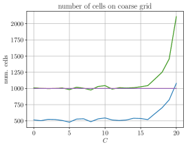
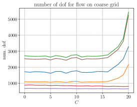
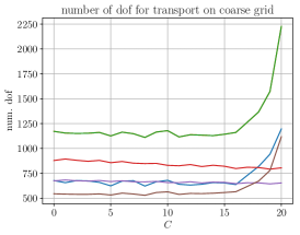
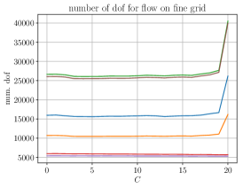
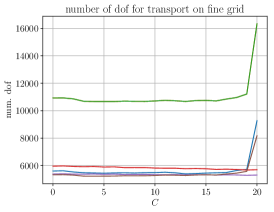
Figure 4: Number of cells (left), number of DOFs for the Darcy problem (middle) and number of DOFs for the dispersion problem (right) against configuration id for the two mesh parameters of Test Case 1, coarse mesh on the top and fine mesh on the bottom grids.

The solution obtained with the scheme mfem is reported, as an example, in Figure 5 on configurations $C0$, $C10$ and $C20$. On the leftmost column the pressure head distribution in the network is shown for the three geometries, whereas the remaining columns depict the temperature distribution $\theta$ at three time-steps corresponding to a time $t=1.25$, $t=2.5$ and $t=5$, respectively. We can notice that, as the trace between fractures $\Omega_{l}$ and $\Omega_{r}$ vanishes, the pressure head distribution displays a steeper gradient around the intersection, and the effective permeability of the network reduces, thus also reducing the penetration depth of the higher temperature zone in the network at fixed time frames. From a computational point of view, simulations become more and more challenging as the solution starts to display steep gradients, especially for methods built on non-conforming meshes, that are not adapted to the geometry, as shown in Figure 6.

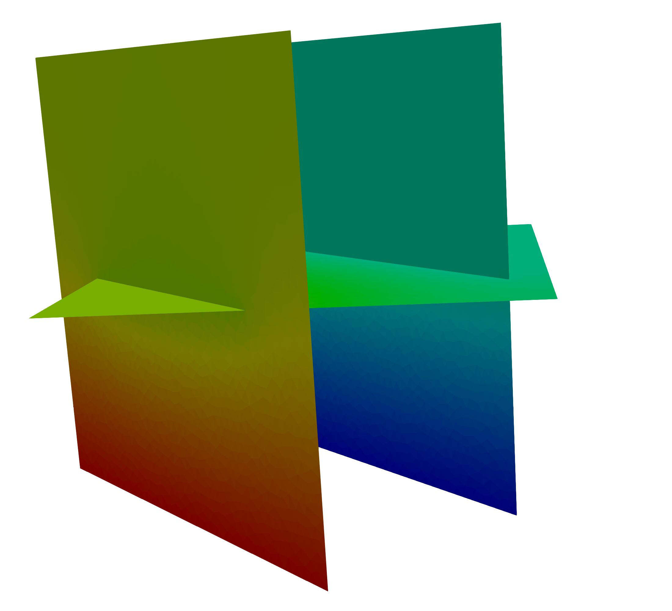
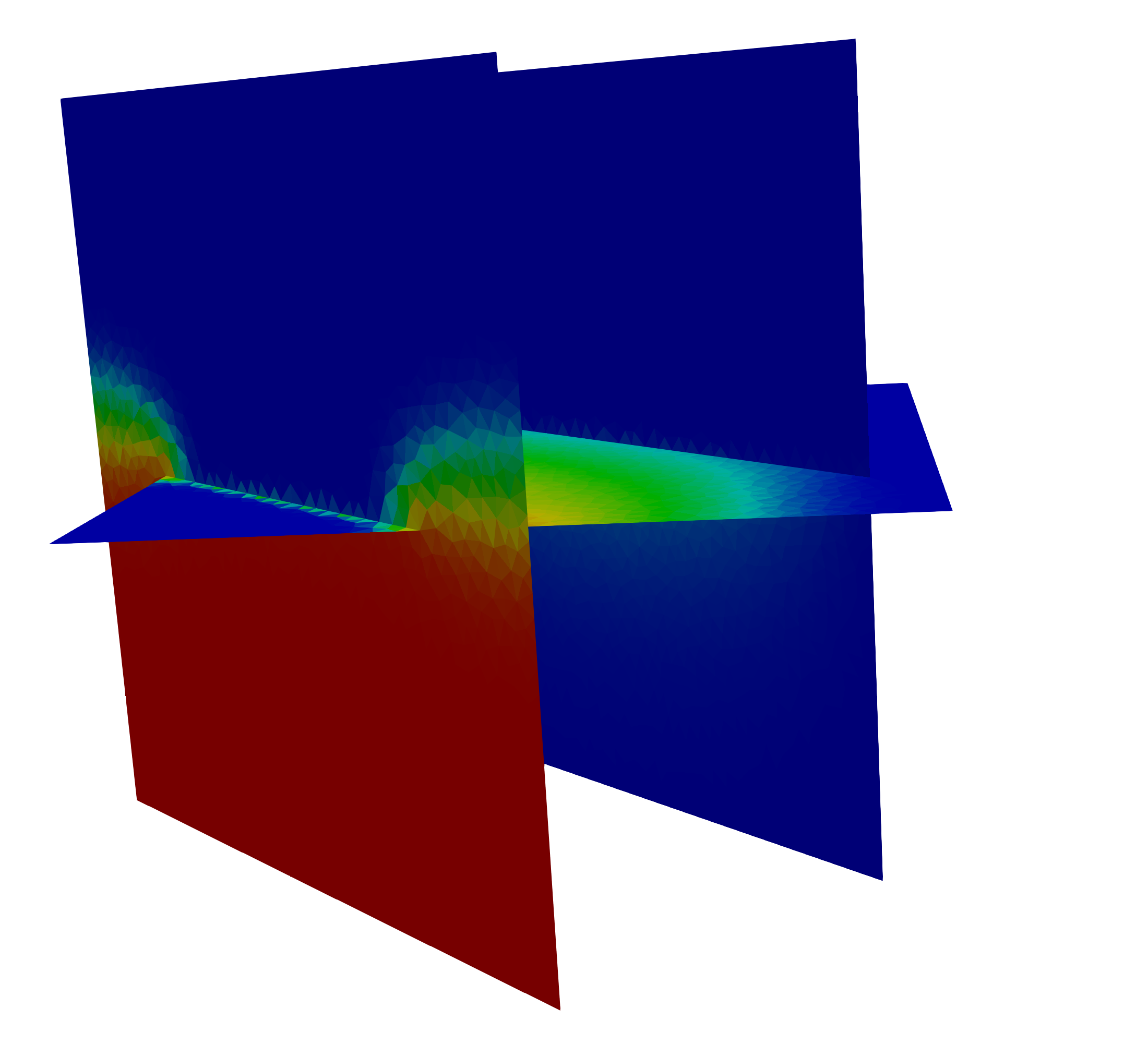
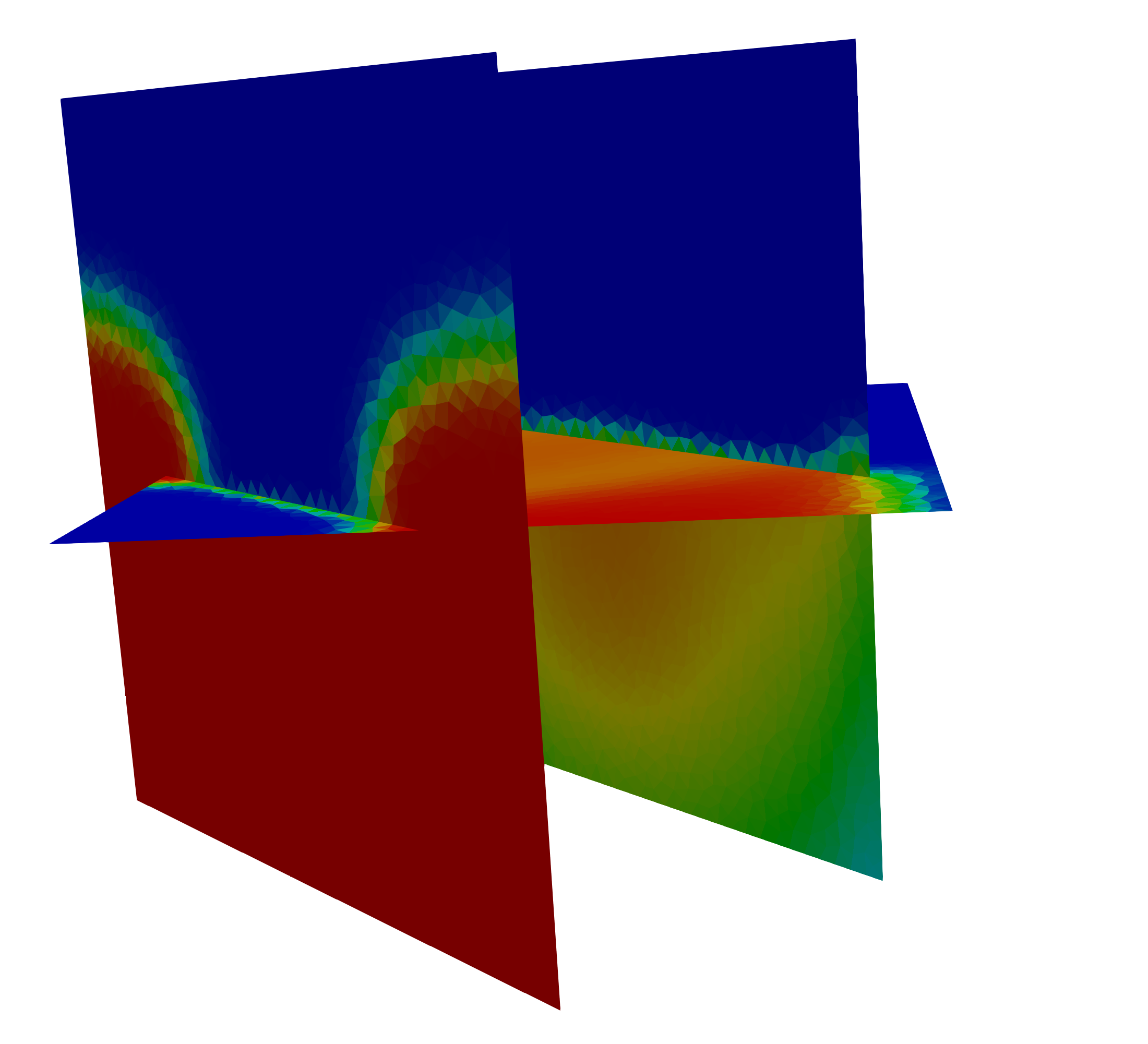
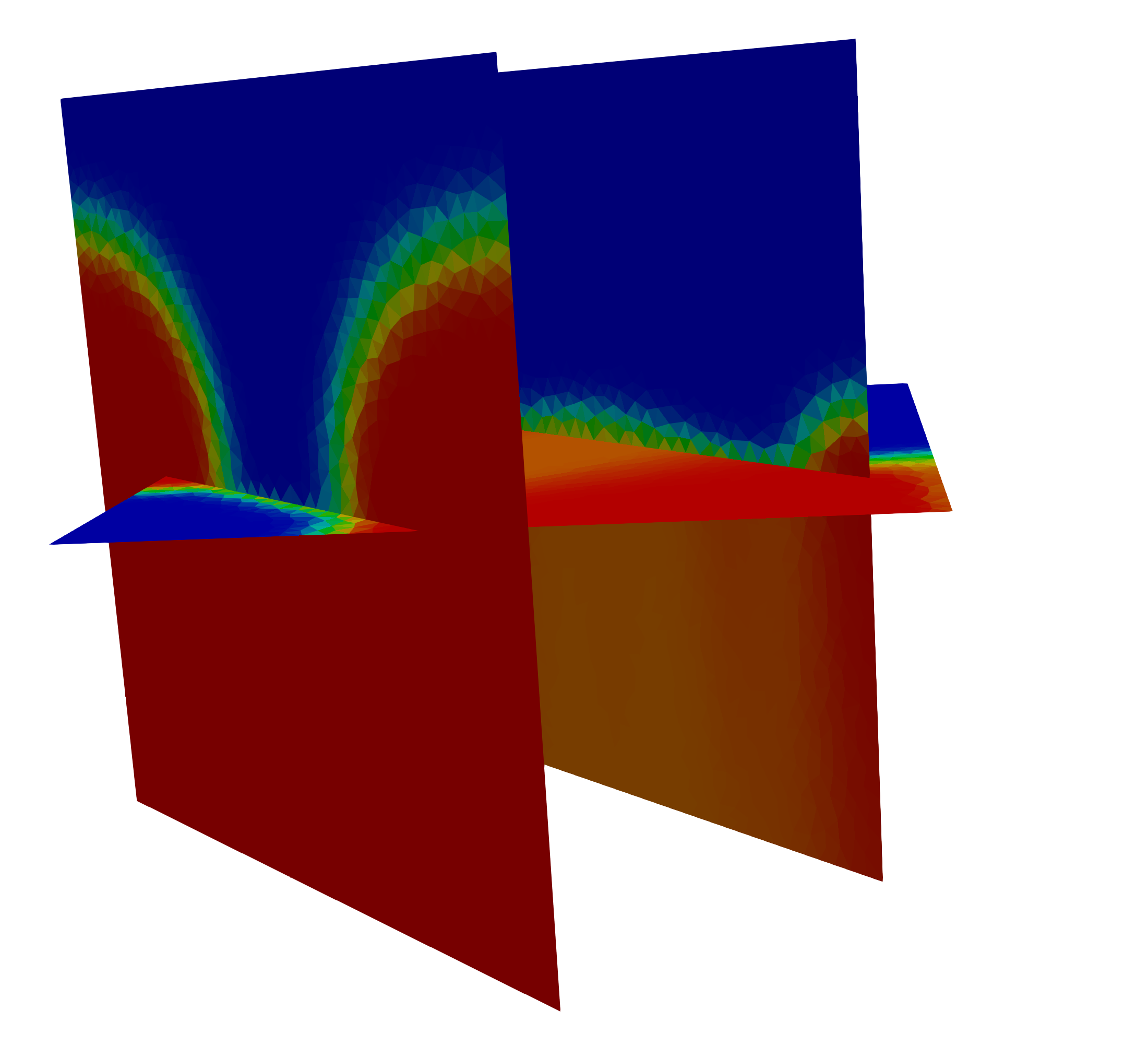
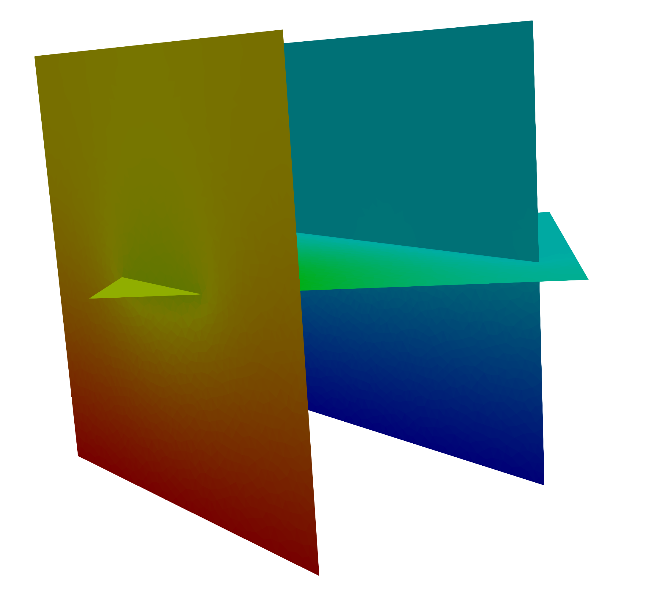
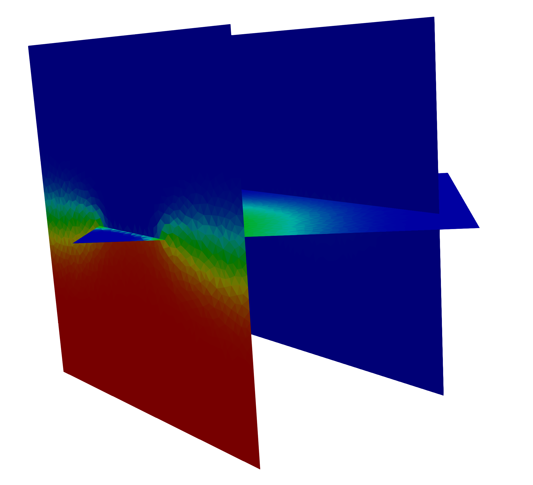
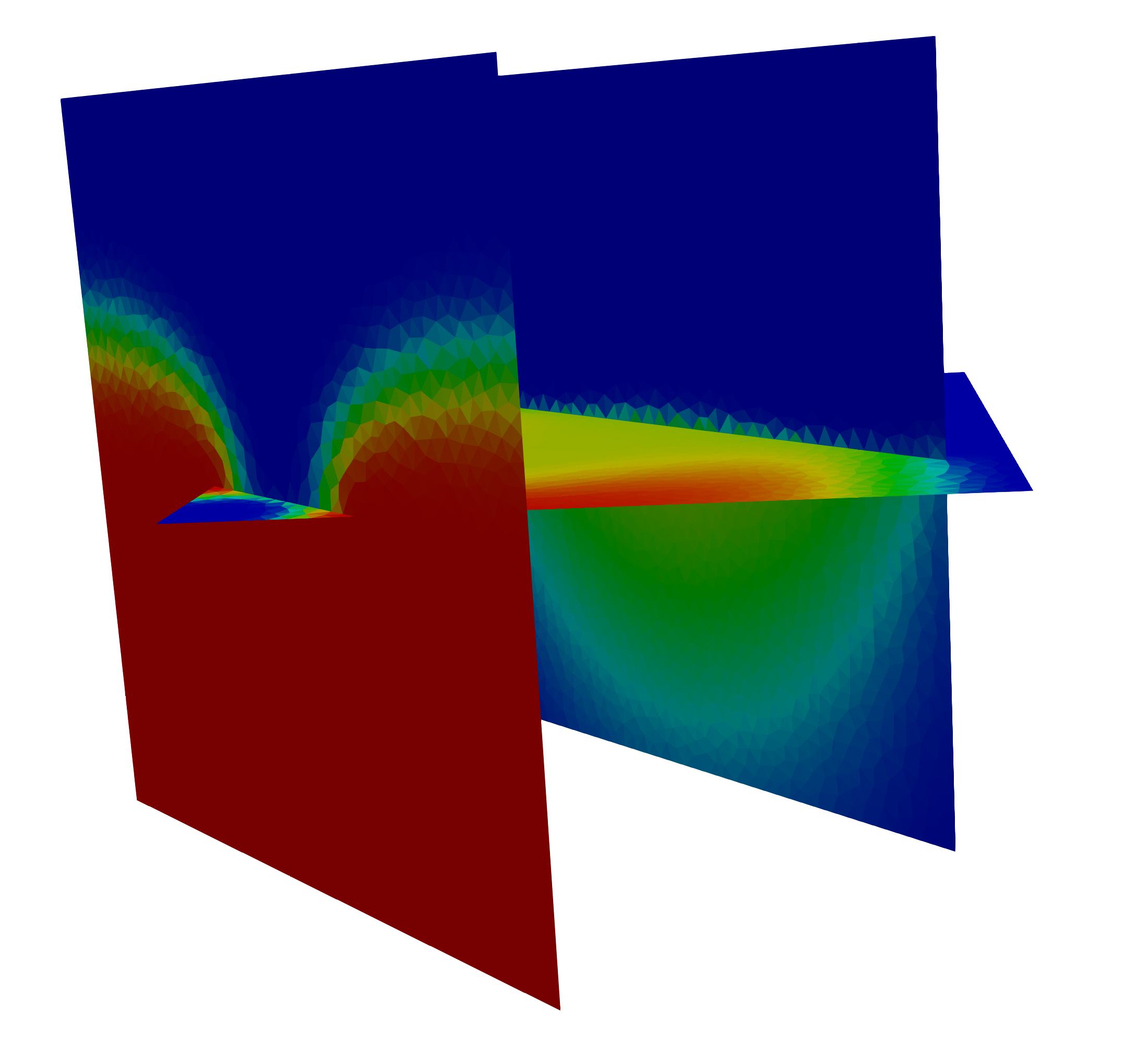
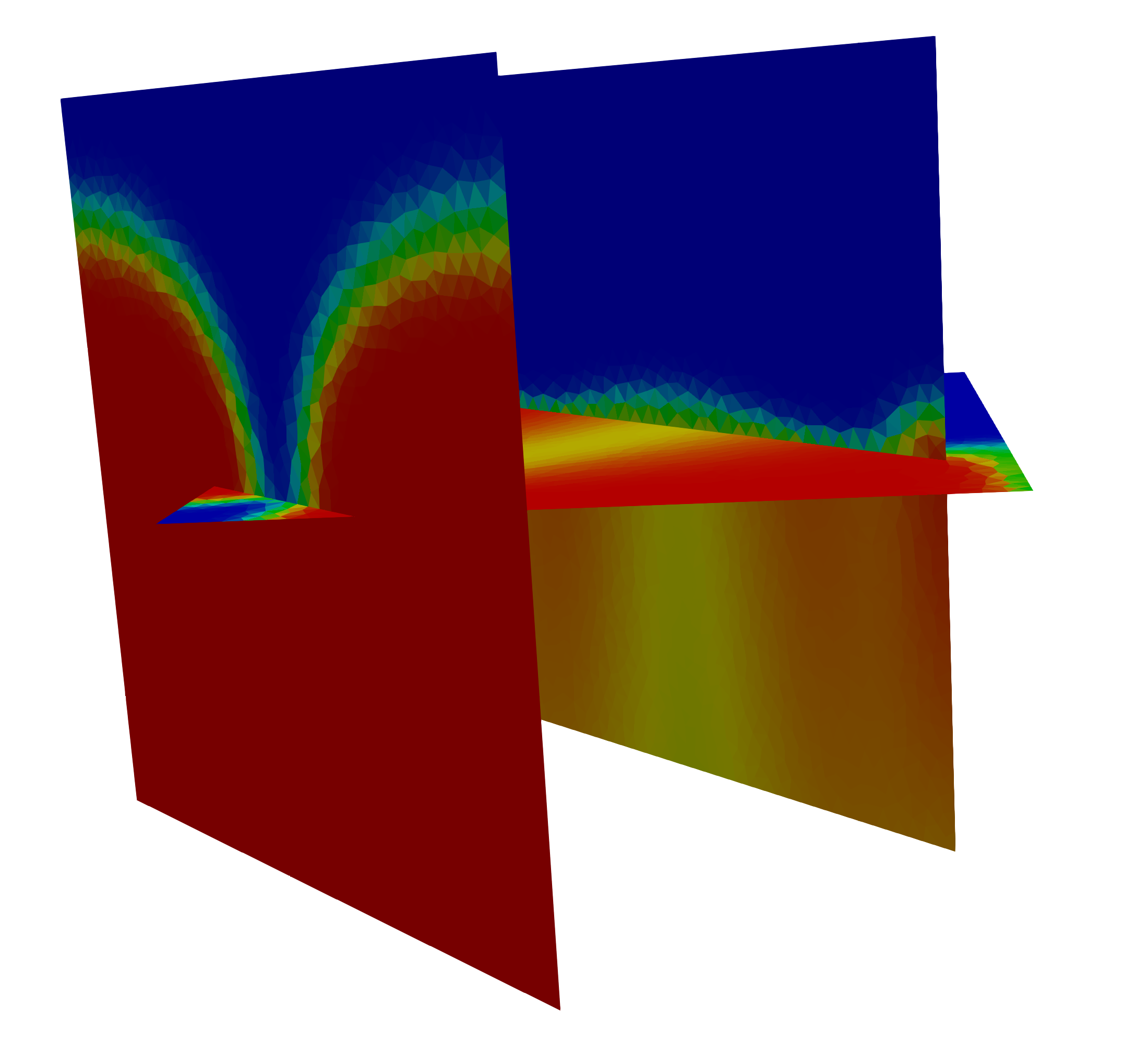
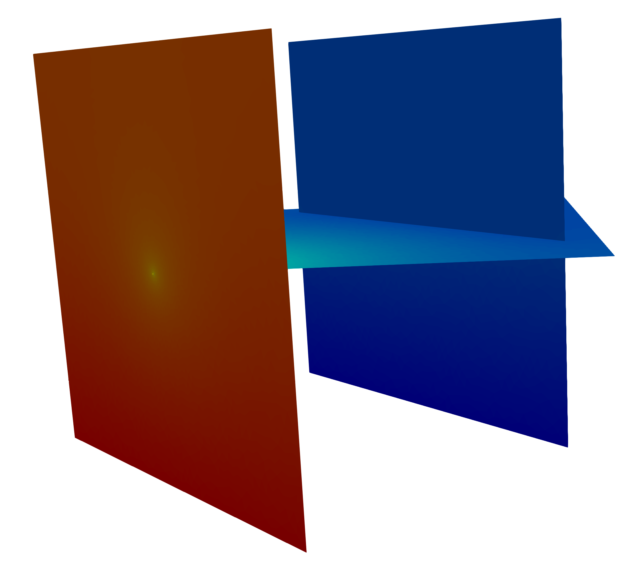
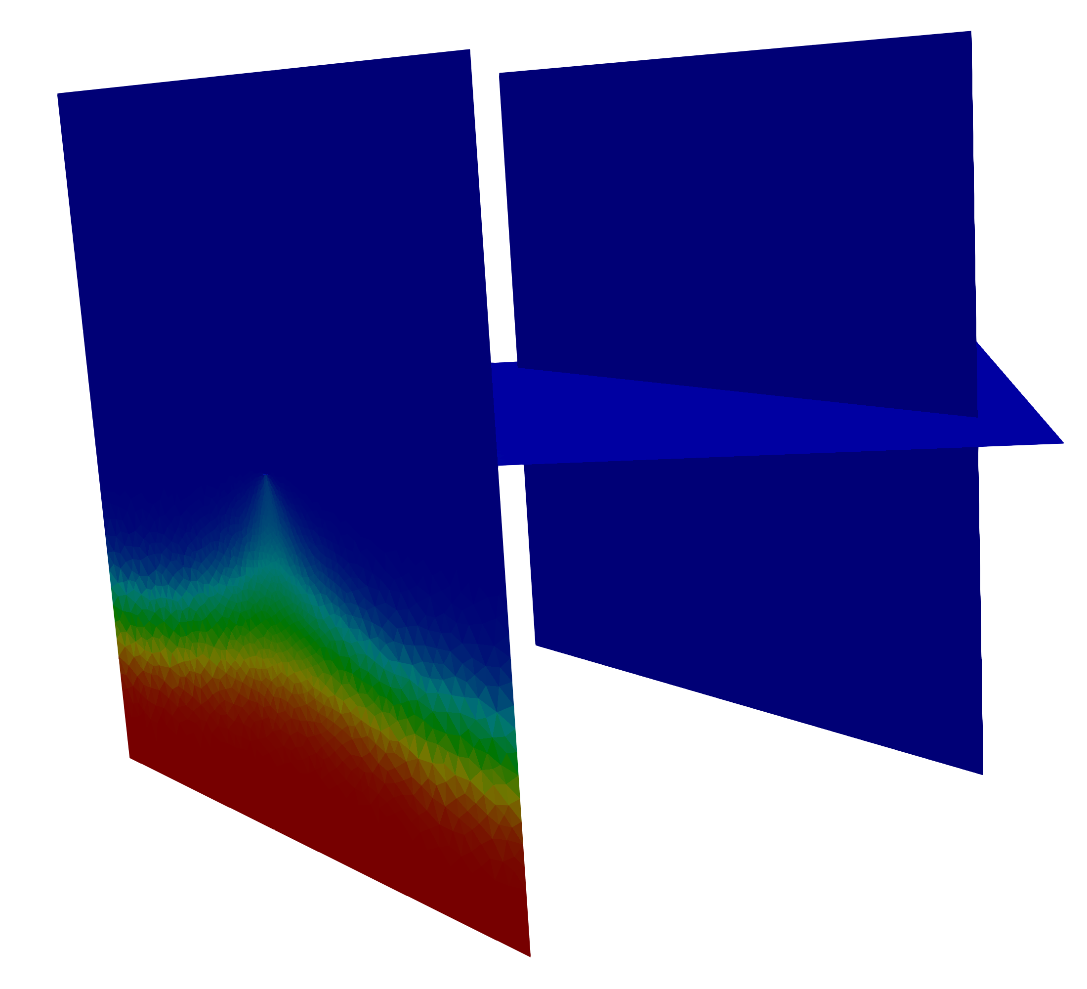
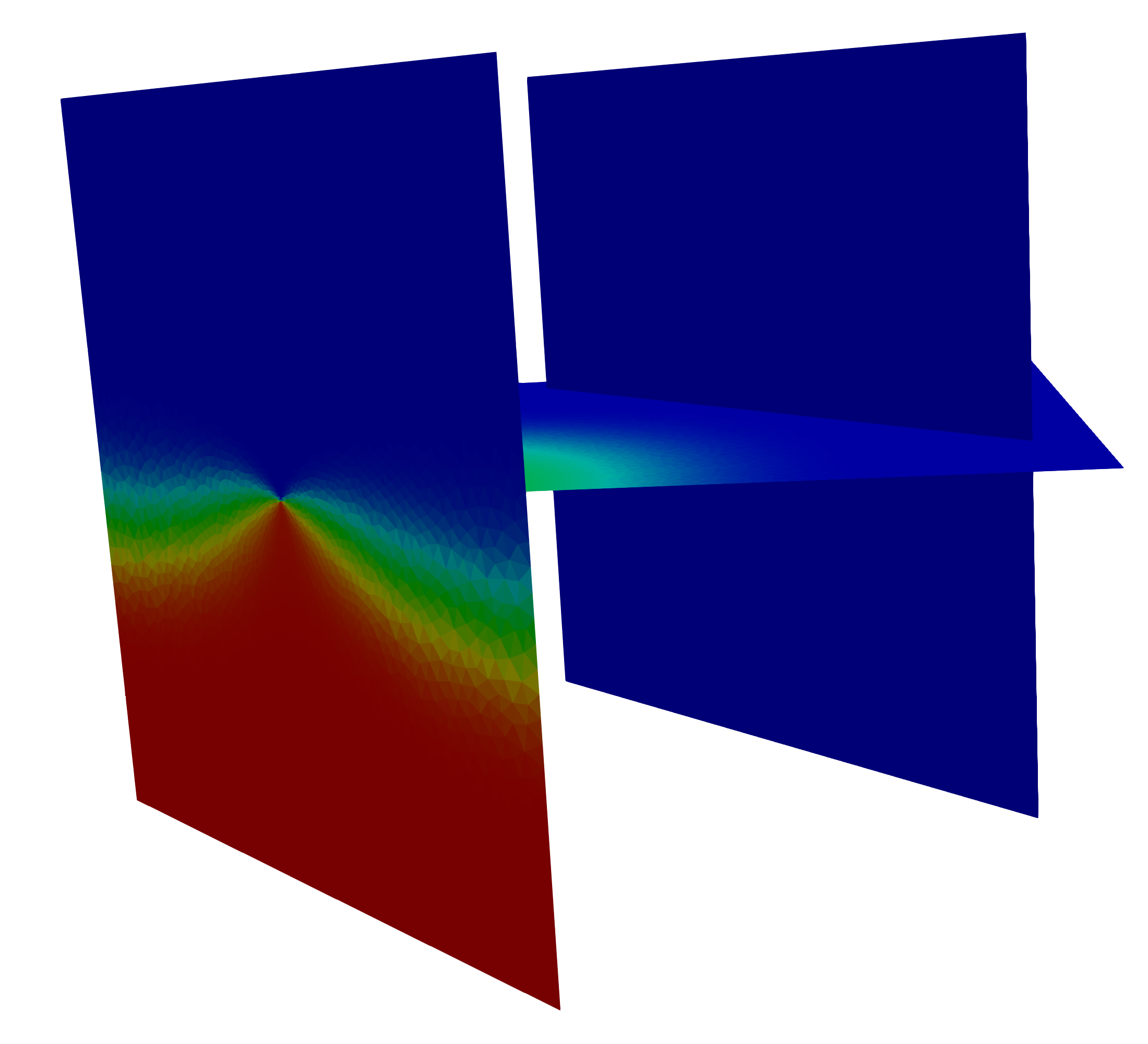
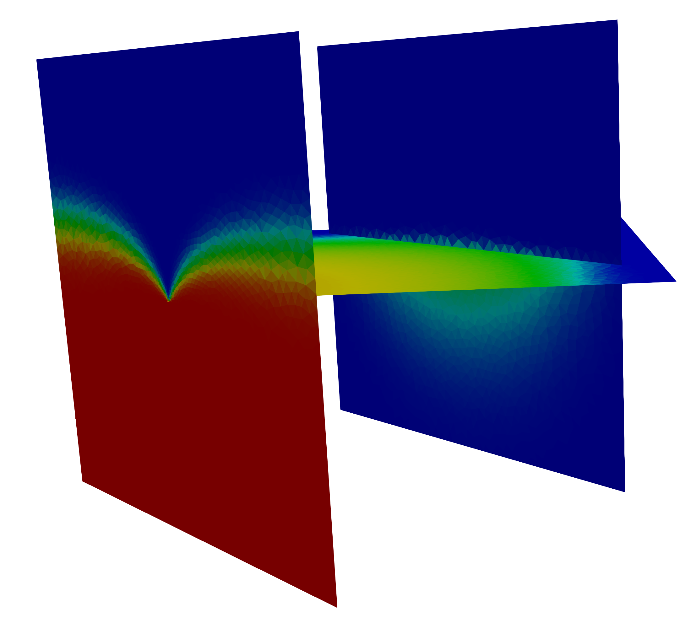
Figure 5: Solution of Test Case 1. On the pressure head solution is shown on the leftmost column at configurations $C0$, $C10$ and $C20$. On the remaining columns the solution $\theta$ is represented at $t=\{1.25,2.5,5\}$, respectively. The colour scale spans from $0$ to $1$.

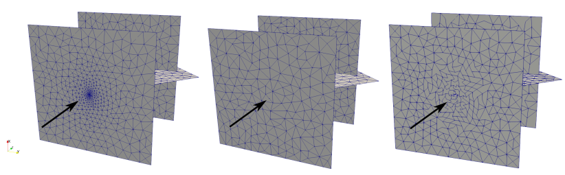
Figure 6: Mesh for Test Case 1 on configuration $C20$ for conforming (left) non-conforming (middle) and coarsened (right) schemes

For all the proposed numerical schemes, at each time-step, the following quantities are computed: the average temperature $\langle{\theta}\rangle_{\Omega}$, the average temperature $\langle{\theta}\rangle_{\mathrm{outflow}}$ on the outflow portion of the boundary, and, for non-locally conservative schemes, as the optimization-based methods, the total flux mismatch $\delta\Phi_{\Gamma}$ at each trace.

A reference solution is computed using the mfem method on a mesh much finer than the three considered here for the simulations, counting about $6.3\times 10^{5}$ cells, almost independently from the configuration id, as cell size is capable of resolving the smallest length of the vanishing trace.

The plots in Figure 7 propose a comparison of average temperature for all the proposed methods against time, on three selected configuration, for all the considered meshes. In the picture, dashed black lines represent relative errors with respect to the reference solution. As expected, all the curves are in very good agreement, also on the coarsest mesh, for configuration $C0$, whereas small discrepancies appear for configuration $C10$ on the coarse mesh that however disappear as the mesh is refined. Larger differences appear, for methods femsupg and xfemsupg, instead for the simulations on configuration $C20$. This is expected, since, as mentioned, when the varying trace becomes very small, methods built on non-matching meshes can not rely on the effect of mesh refinement around the vanishing trace which clearly improves representation capabilities of conforming methods. We observe that method mvemup retains good approximation capabilities despite the coarsening.

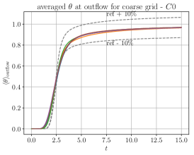
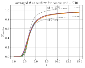
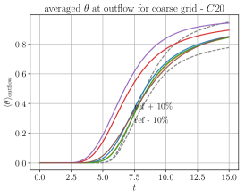
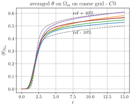
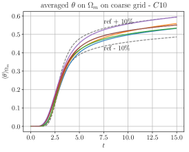
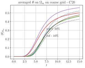
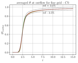
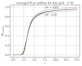
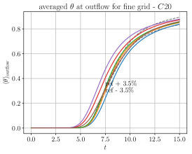
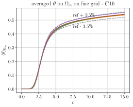
Figure 7: Average temperature on curves against time for Test Case 1 on the coarsest (first six pictures) and finest (last six pictures) for selected fracture and configurations. Columns refer to the same geometrical configuration: $C0$ on column 1, $C10$ on column 2 and $C20$ on column 3. The average temperature curves refer to fracture $\Omega_{m}$.

In order to quantify what is the effect of mesh adaptation due to conformity requirements on the quality of the solution with respect to the effect of the approximations introduced by the non-matching schemes themselves, in Figure 8 (left) the outflow average temperature for the methods opt-xfem and opt-fem is reported against time, for configuration $C20$ on a perturbation of the coarse mesh used for the conforming methods for configuration $C20$, overlapped to the curves of the other schemes, in transparency, on the original meshes. We observe that the curves of methods opt-fem and opt-xfem on the perturbed adapted mesh are now much closer to the curves of other conforming approaches, thus clearly showing the effect of mesh adaptation on the quality of the solution. The solution obtained with the opt-xfem approach on the perturbed mesh at $t=15$ is reported in Figure 8, on the right, along with a detail of the mesh around $\Gamma_{0}$, clearly showing the non conformity of the mesh. Two aspects are to be remarked: first, the non-conforming approaches are capable of producing reasonable approximations of the solution also on the coarse mesh, which can be greatly improved refining the mesh and still using a fraction of the degrees of freedom required by the conforming approaches, see, e.g., the last two plots in the third column of Figure 7; second, non-conforming approaches allow to freely choose the refinement level of the mesh, thus allowing to efficiently use mesh adaptation strategies, only refining the mesh where required, independently of the geometrical constraints [14].

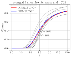
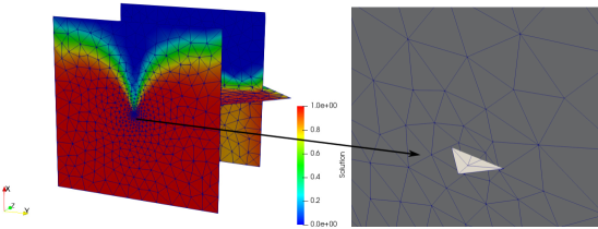
Figure 8: Outflow average temperature curve with opt-xfem and opt-fem approaches (left), and solution with opt-xfem at $t=15$ with a zoom of the mesh around $\Gamma_{0}$ (right), both on on the perturbed mesh of configuration $C20$.

As the non-conforming approaches opt-xfem and opt-fem are non locally conservative, Figure 9 report the value of $\delta\Phi$ against time on the coarsest mesh for the two traces of this example at configurations $C0$, $C10$ and $C20$, from left to right, respectively, results with the opt-xfem approach are on the top, results with opt-fem on the bottom. The maximum-in-time absolute values of the total flux on traces $\Gamma_{0}$ and $\Gamma_{1}$ are reported in Table 2, computed on the finest mesh as $\Phi_{\Gamma_{0}}=\max_{t}\frac{1}{2}\left(\Phi_{\Gamma_{0},l}+\Phi_{\Gamma_{0},c}\right)$, and $\Phi_{\Gamma_{1}}=\max_{t}\frac{1}{2}\left(\Phi_{\Gamma_{1},c}+\Phi_{\Gamma_{1},r}\right)$. We can see that relative values of less than $1\%$ are obtained for all times for both methods, with the higher values corresponding to the configuration $C20$, as expected. Moreover, for the larger times, mismatch values tend to decrease or to remain constant at a fixed value. Thus this non-local-conservation has a negligible impact on the computed solution. Further, mismatch errors can be reduced by refining the mesh.

The mesh Péclet number for this problem ranges between a maximum of about $6\times 10^{2}$ to a minimum of about $100$ on the computational meshes for opt-xfem, opt-fem and mfem methods, thus a Streamline-Upwind-Petrov-Galerkin (supg) stabilization strategy was adopted. As a consequence small overshoots/undershoots in the solution are observed in supg stabilized methods, as well known in the literature, whereas the intrinsic diffusive behavior of methods using upwinding for advection prevents this kind of phenomena.

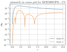
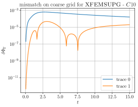
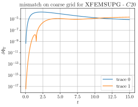
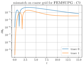
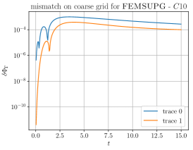
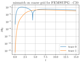
Figure 9: Total flux mismatch against time for Test Case 1 on traces $\Gamma_{0}$ (top) and $\Gamma_{1}$ (bottom) for configuration $C0$ (left), $C10$ (middle) and $C20$ (right)

Table 2: Maximum value in time of total fluxes $\Phi_{\Gamma_{0}}$ and $\Phi_{\Gamma_{1}}$ on traces $\Gamma_{0}$ and $\Gamma_{1}$ of Test Case 1, respectively, computed with the xfemsupg method on configurations $C0$, $C10$ and $C20$.

	$C0$	$C10$	$C20$
$\Phi_{\Gamma_{0}}$	0.6072	0.4725	0.251
$\Phi_{\Gamma_{1}}$	0.876	0.912	1.300

4.2 Synthetic network

In the second test, labeled Test Case 2, we consider a more complex network composed of 10 fractures with 14 traces, thus being more similar to (a portion of) realistic DFNs, still remaining simple enough to perform analyses on the solutions obtained with the considered schemes. The network is represented in Figure 10, where the inflow and outflow portions of the boundary are also marked. Also in this case the Darcy velocity $\bm{u}$ is first computed solving problem 2 or 4, depending on the chosen numerical scheme, with constant hydraulic conductivity equal to one on all fractures and null source term. A unitary pressure head drop is imposed between the inflow and outflow portions of the border, all other fracture edges being insulated. The Darcy velocity is then used as an input for an advection-diffusion problem for a scalar quantity $\theta$, as formulated in 6, with null source and reaction terms. A coefficient $\zeta=1$ is chosen, whereas the diffusion coefficient is $D=10^{-4}$. A unitary Dirichlet boundary condition is prescribed on the inflow border and all other edges are insulated.

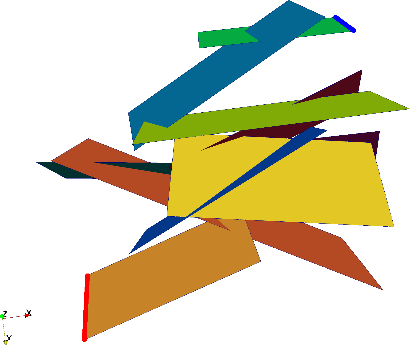
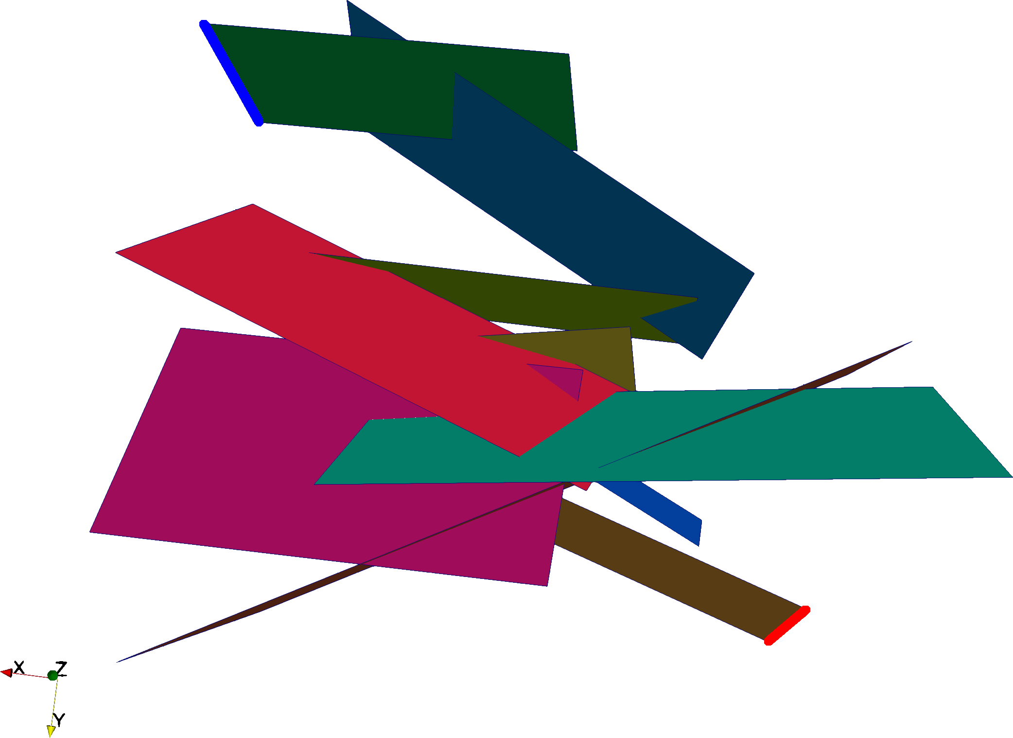
Figure 10: Geometry of Test Case 2 and two views of the network. A red line represents the inflow and a blue thick line the outflow part of the boundary, respectively.

Two meshes are used also for Test Case 2 counting about $10^{3}$ elements (coarse mesh) and $4\times 10^{4}$ elements (fine mesh), respectively. The mesh Péclet number, related to the coarse mesh for supg stabilized methods, is of about $100$. An equally-spaced mesh is then used for time discretization with $500$ steps of length $0.05$. Also in this case, the initial solution is the null function. An example of the obtained numerical solution with the tpfa method is shown in Figure 11: in the first column on the left the pressure head distribution in the network is represented, solution of the Darcy problem on the coarse (top) and fine (bottom) meshes; the remaining columns depict the solution $\theta$ of the dispersion problem at three selected time frames, corresponding to $t=3.35$, $t=6.25$ and $t=12.5$, again on the coarse (top) and fine (bottom) mesh. Coherently the heat flows from the inflow to the outflow by following a tortuous path given by the complex disposition of the fractures and traces. The solution on the coarse grid has a spreader front than on the fine grid due to the artificial diffusivity of the scheme.

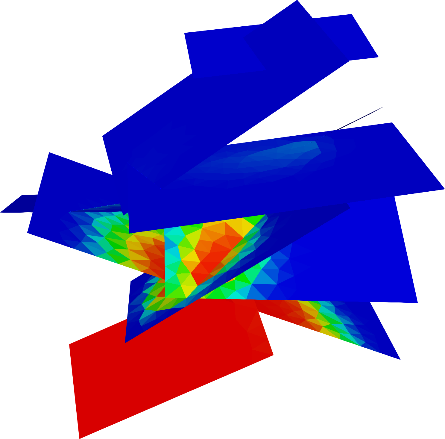
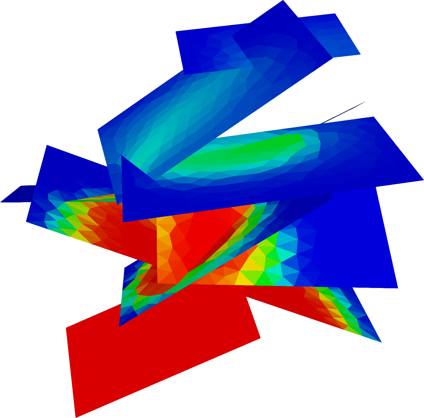
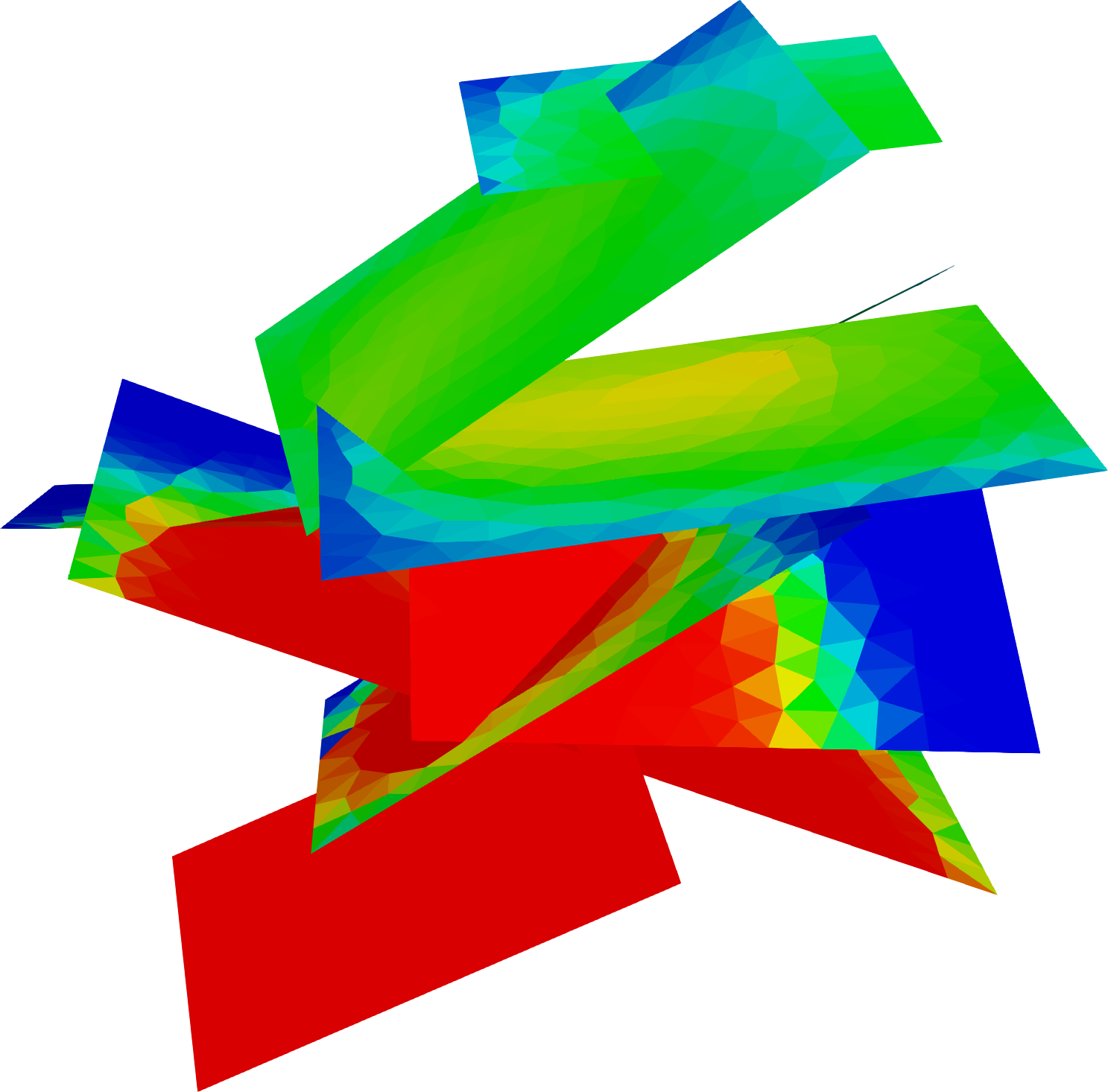
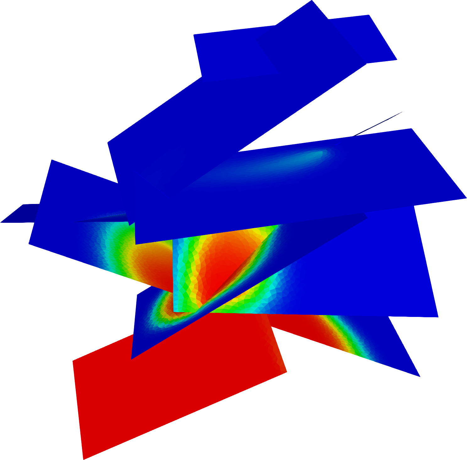
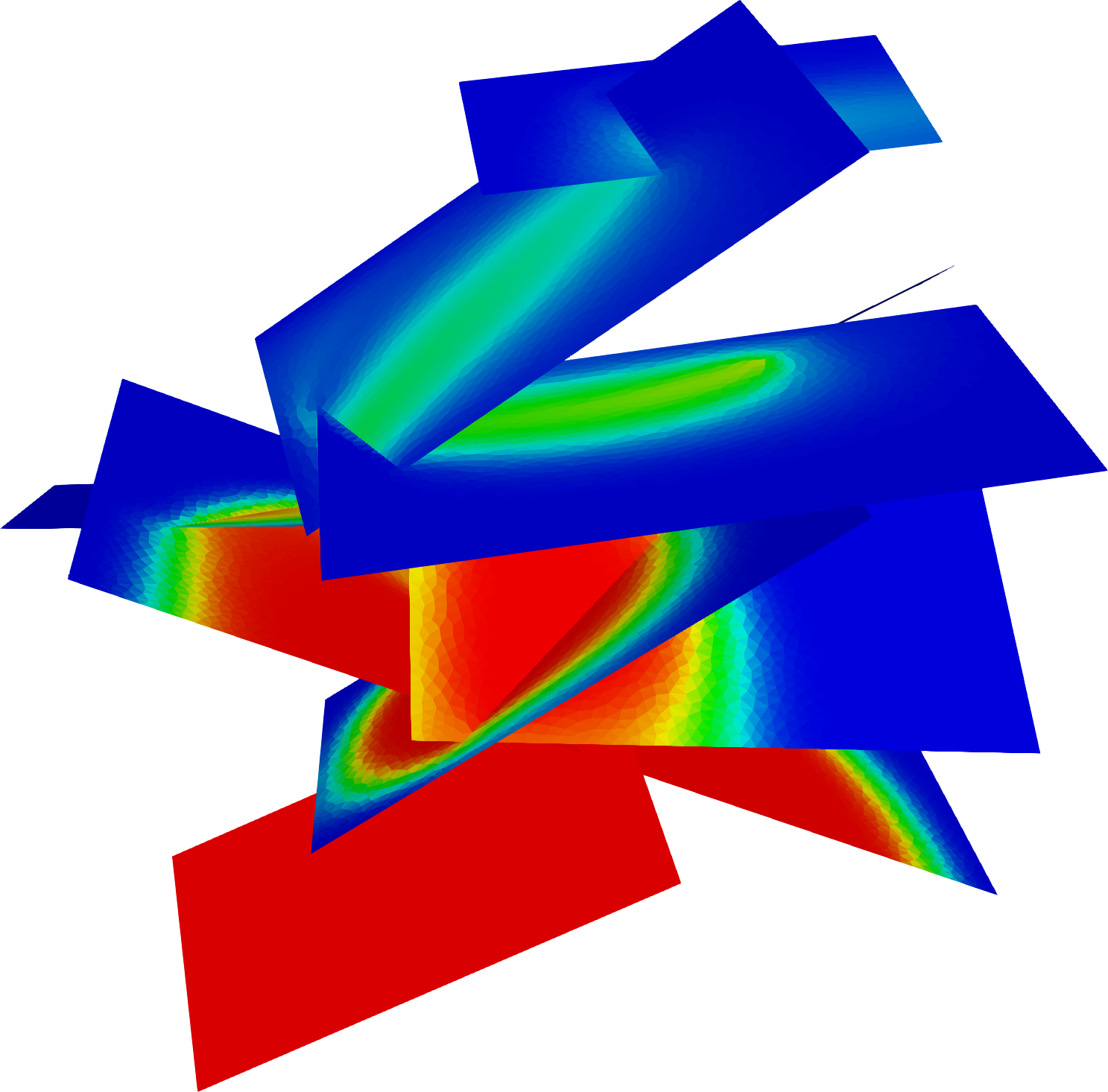
Figure 11: Solution of the test case in Subsection 4.2. On the first column the pressure head solution for the two grid refinements. The other columns show $\theta$ at different time: 3.35, 6.25, and 12.5, respectively, for both level of refinement. In all cases the solution is rescaled in the range $[0,1]$.

As previously, the average temperature $\langle{\theta}\rangle_{\Omega}$ on selected fractures, the average outflow temperature $\langle{\theta}\rangle_{\mathrm{outflow}}$ and flux mismatch $\delta\Phi_{\Gamma}$ at traces are used to compare and assess the approximation capabilities of the various schemes. The curves of $\langle{\theta}\rangle_{\Omega_{1}}$, $\langle{\theta}\rangle_{\Omega_{3}}$ and $\langle{\theta}\rangle_{\mathrm{outflow}}$ are reported in Figure 12. A reference solution is computed with the mfemsupg method on a mesh counting about $2\times 10^{4}$ cells, and relative error curves with respect to this solution are shown in dashed lines in the Figure 12. We can observe that, despite the network has a larger number of fractures and fracture intersections with respect to Test Case 1, all the methods, in absence of severe geometrical features have good approximation properties, that further improve with mesh refinement. The larger differences are observed for the average outflow temperature curve related to the mvemup approach on the coarse mesh and for the average temperature curves of femsupg again on the coarse mesh. In both cases differences slightly exceed $10\%$ of the reference, and are reduced by mesh refinement. Concerning the mvemup the difference is caused by the coarsening process which reduces the number of elements of the original mesh to about one half. Also, the tpfa method used for advection is observed to have poor performances on irregular polygonal cells, as the ones generated by the coarsening method. Concerning the femsupg method, some discrepancies with respect to the reference are to be expected, as the approach is designed to be computationally inexpensive, nonetheless it is capable of providing satisfactory predictions.

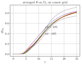
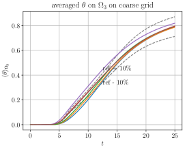
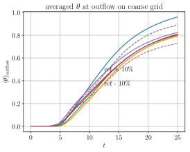
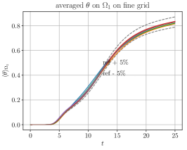
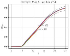
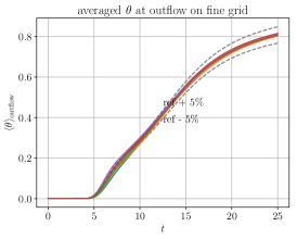
Figure 12: Average temperature on two selected fractures (left and middle columns) and at outflow (right column) curves against time for Test Case 2. Coarse mesh on top, fine mesh at the bottom.

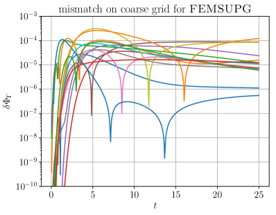
Figure 13: Total flux mismatch against time for all the traces of the network of Test Case 2 on the coarse mesh with methods femsupg (left) and xfemsupg (right).

Curves of the total flux mismatch at the traces are reported against time in Figure 13 for the femsupg and xfemsupg methods. In this picture values of $\delta\Phi_{\Gamma}$ are shown, without labels, for all the traces in the network, highlighting that, in all cases, the errors remain limited in time. Further, maximum-in-time mismatch values are lower than $1\%$ of the total flux, for all the traces; values of the maximum flux with respect to time on each trace are reported in Table 3, computed with the xfemsupg method on the finest mesh.

Table 3: Maximum value in time of total flux across each trace of the DFN for Test Case 2 computed with the xfemsupg method on the fine mesh.

$\Phi_{\Gamma_{1}}$	$\Phi_{\Gamma_{2}}$	$\Phi_{\Gamma_{3}}$	$\Phi_{\Gamma_{4}}$	$\Phi_{\Gamma_{5}}$	$\Phi_{\Gamma_{6}}$	$\Phi_{\Gamma_{7}}$
0.040	0.079	0.150	0.260	0.284	0.047	0.074
$\Phi_{\Gamma_{8}}$	$\Phi_{\Gamma_{9}}$	$\Phi_{\Gamma_{1}0}$	$\Phi_{\Gamma_{1}1}$	$\Phi_{\Gamma_{1}2}$	$\Phi_{\Gamma_{1}3}$	$\Phi_{\Gamma_{1}4}$
0.020	0.393	0.163	0.443	0.061	0.058	0.063

4.3 Extruded real outcrop

In this last test case we consider a fracture network generated from an extruded outcrop, located in Western Norway. The test case is inspired by Section 4.4 of [32]. The network is composed by 89 intersecting fractures resulting in 166 traces. There are 7 non-connected fractures and with no flow boundary conditions, which will not contribute to the solution. The geometry is depicted in Figure 14. The aim of this test case is to validate the proposed numerical schemes in presence of realistic physical parameters of a real fracture network. However, we assume that all the fractures share the same values of hydraulic conductivity and heat diffusion coefficient.

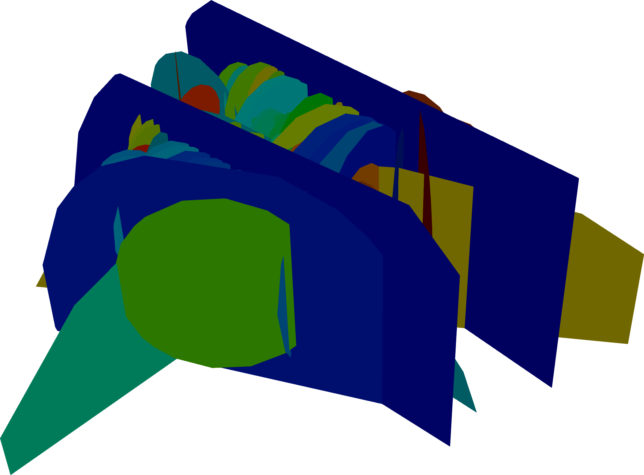
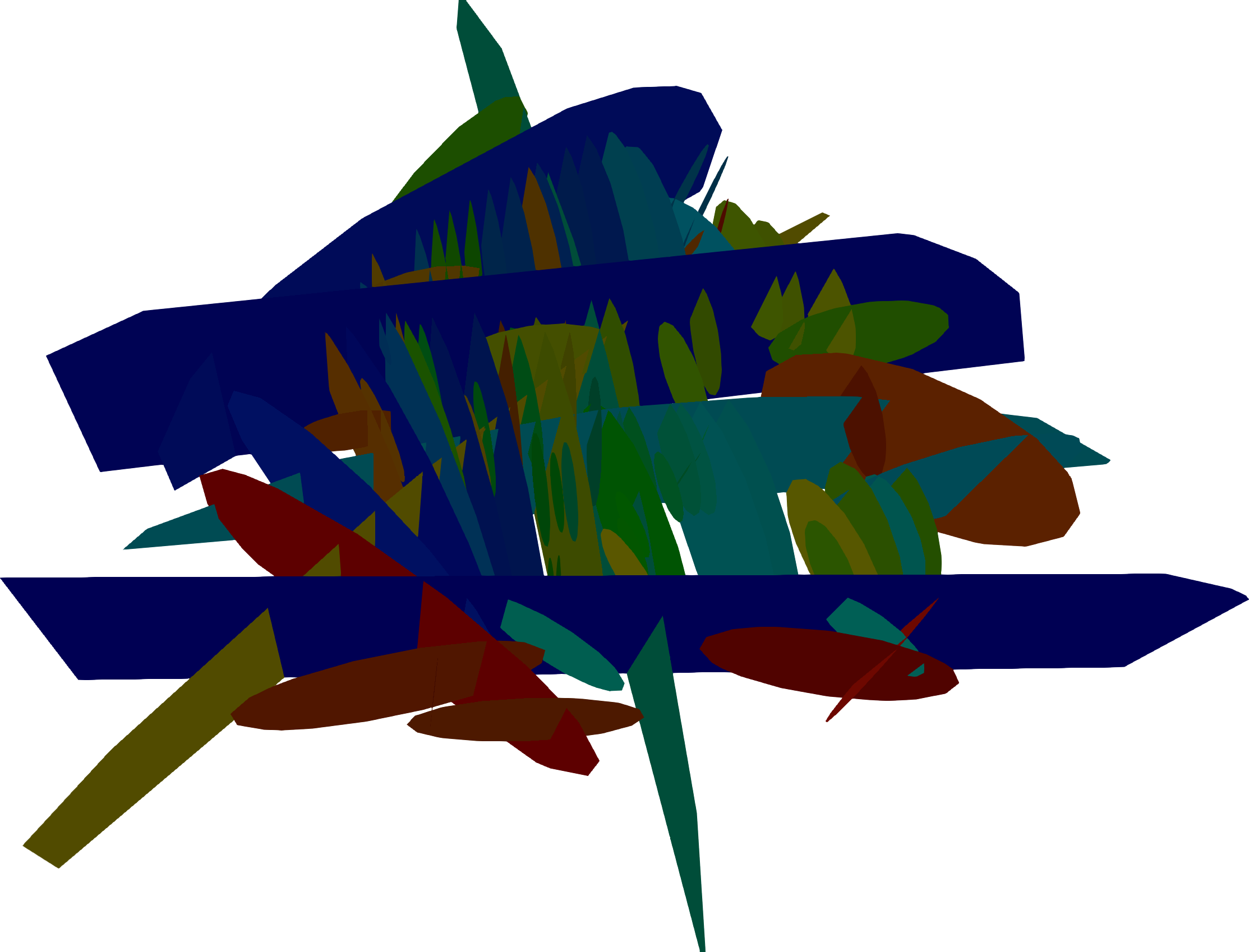
Figure 14: Geometry of the test case in Subsection 4.3. On the top two screenshot of the geometry of the network. On the bottom a sketch of the network with only the largest fractures to present the boundary conditions: on the left in the case of inflow and outflow imposed on two different fractures, on the right on the same fracture. The inflow is represented in red and the outflow in blue.

We consider two distinct problems, that differ from each other from the position of the inflow and outflow boundaries. In the first case (denoted as case 1) the inflow and outflow are imposed on two different fractures, while in the second case (case 2) they belong to the same fracture. See Figure 14 where a sketch of the network is shown with the position of the inflow and outflow boundaries. On the other portions of the boundaries a no flow boundary condition is given. In both cases, we require a simulation grid with roughly 70k elements.

Fractures are immersed in granite and we assume that at the beginning of the simulation the water contained in the fractures is at $353.15\text{\,}\mathrm{K}\text{/}$ ($80\text{\,}\mathrm{\SIUnitSymbolCelsius}\text{/}$). The relations to compute the physical parameters for the simulations are the ones presented in Subsection 2.2. We assume $\epsilon_{i}=$2\text{\,}\mathrm{mm}\text{/}$$ $\forall i$, and $\phi_{i}=0.95$ $\forall i$. The water and rock physical parameters are reported in Table 4.

	Water	Rock
Dynamic viscosity	$\mu=$3.55\text{\,}\mathrm{Pa}\text{\,}\mathrm{s}\text{/}$$	–
Thermal conductivity	$\lambda_{w}=$0.667\text{\,}\mathrm{W}\text{/}\text{(}\mathrm{m}\text{\,}\mathrm{K}\text{)}$$	$\lambda_{m}=$3.07\text{\,}\mathrm{W}\text{/}\text{(}\mathrm{m}\text{\,}\mathrm{K}\text{)}$$
Density	$\rho_{w}=$1000\text{\,}\mathrm{kg}\text{/}{\mathrm{m}}^{3}$$	$\rho_{m}=$2700\text{\,}\mathrm{kg}\text{/}{\mathrm{m}}^{3}$$
Specific heat capacity	$c_{w}=$4099\text{\,}\mathrm{J}\text{/}\text{(}\mathrm{kg}\text{\,}\mathrm{K}\text{)}$$	$c_{m}=$790\text{\,}\mathrm{J}\text{/}\text{(}\mathrm{kg}\text{\,}\mathrm{K}\text{)}$$
Heat transfer coefficient	$\gamma=$1.25\text{\times}{10}^{-3}\text{\,}\mathrm{W}\text{/}\text{(}{\mathrm{m}}^{2}\text{\,}\mathrm{K}\text{)}$$

Table 4: List of rock and water coefficients for the example in Subsection 4.3.

From these data we obtain, $\forall i=1,\ldots,N_{\Omega}$,

$$K_{i} \approx$1.84\text{\times}{10}^{-6}\text{\,}{\mathrm{m}}^{2}\text{/}\mathrm{s}$\,, c_{e,i} \approx$4\,000\,700\text{\,}\mathrm{J}\text{/}\text{(}{\mathrm{m}}^{3}\text{\,}\mathrm{K}\text{)}$\,,$$

$$\lambda_{e,i} \approx$0.72\text{\,}\mathrm{W}\text{/}\text{(}\mathrm{m}\text{\,}\mathrm{K}\text{)}$\,, \zeta_{i} \approx$1.95\text{\times}{10}^{-3}\text{\,}\mathrm{m}\text{/}$\,,$$

$$D_{i} \approx$0.35\text{\times}{10}^{-9}\text{\,}{\mathrm{m}}^{3}\text{/}\mathrm{s}$\,, \iota_{i} \approx$3.05\text{\times}{10}^{-10}\text{\,}\mathrm{m}\text{/}\mathrm{s}$\,.$$

Regarding boundary conditions, for the Darcy problem we impose a pressure head equal to $2.5\text{\,}\mathrm{km}\text{/}$ at the inflow boundary and $0\text{\,}\mathrm{m}\text{/}$ at the outflow boundary, while for the heat problem we impose $303.15\text{\,}\mathrm{K}\text{/}$ ($30\text{\,}\mathrm{\SIUnitSymbolCelsius}\text{/}$) at the inflow and zero diffusive flux at the outflow. The simulation time is a year ($3.154\text{\times}{10}^{7}\text{\,}\mathrm{s}\text{/}$), divided in 200 time steps.

The conforming computational mesh counts about $7\times 10^{4}$ elements, while the non-matching computational mesh has $2\times 10^{4}$ cells and are shown in Figure 15. It is possible to notice, how, in order to meet the conformity requirement, mesh elements of the conforming mesh are concentrated near the traces, whereas, the non-matching mesh has all elements of equal size evenly distributed in the network. The non matching mesh is characterized by a mesh Péclet number of about $3\times 10^{4}$ for case 1 and $6.6\times 10^{4}$ for case 2, reached on fracture $\Omega_{0}$, in both cases. The non-adapted mesh and the high mesh Péclet number make this example extremely complex for methods built on non-conforming meshes and relying on stabilization for advection dominated flow regimes.

The computed solution with the mfemup scheme is reported in Figure 16 where we display the solution of the Darcy problem on the left and the solution at the end of time evolution on the right, for both the setting of case 1, on top and case 2, at the bottom.

Figure 17 shows the curves against time of the average temperature on the inflow ($\Omega_{0}$) and outflow ($\Omega_{1}$) fractures, along with the average temperature on the outflow boundary. Despite the complexity of the geometry and of the model, curves appear in good agreement. For this last example no coarsening was used for the mvemup method, as the poor performances of the tpfa method on polygonal cells, already observed in Test Case 2, have a strong impact on the quality of the solution in this more complex case. The curves related to the mvemup approach on triangular meshes are almost perfectly overlapped to the curves of the mfemup method. Curves of xfemsupg and femsupg are in good agreement with those of the other methods.

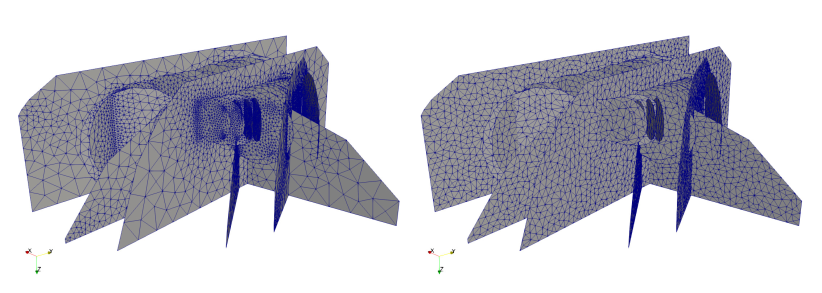
Figure 15: Conforming (left) and non-matching (right) mesh for Test Case 3

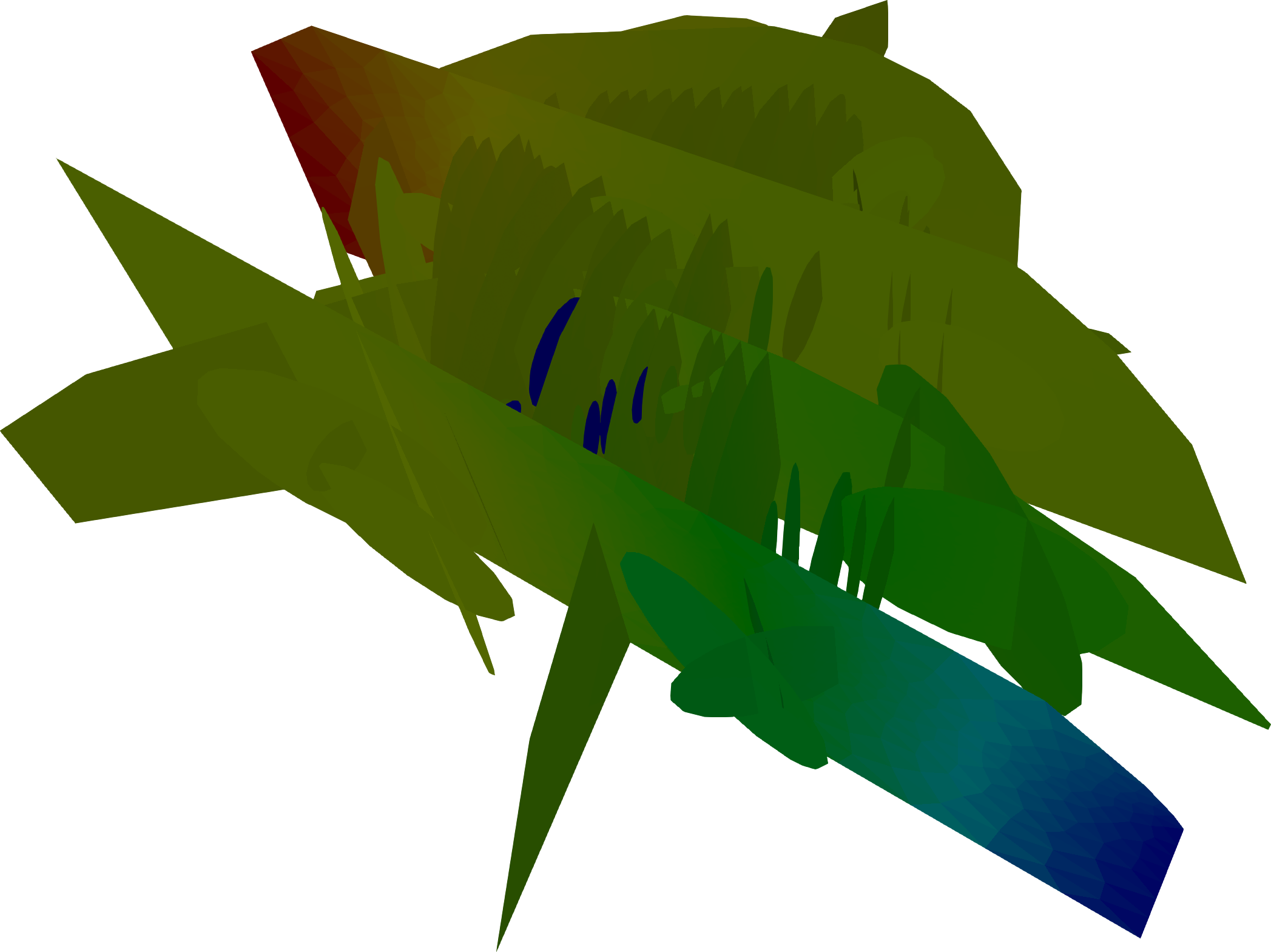
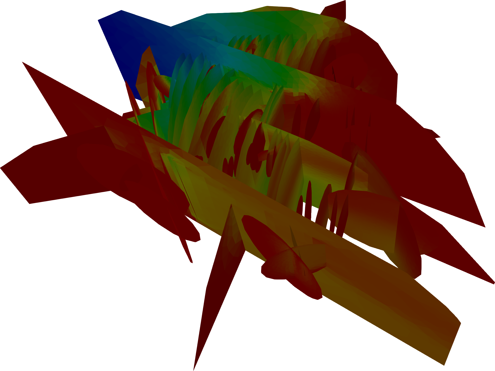
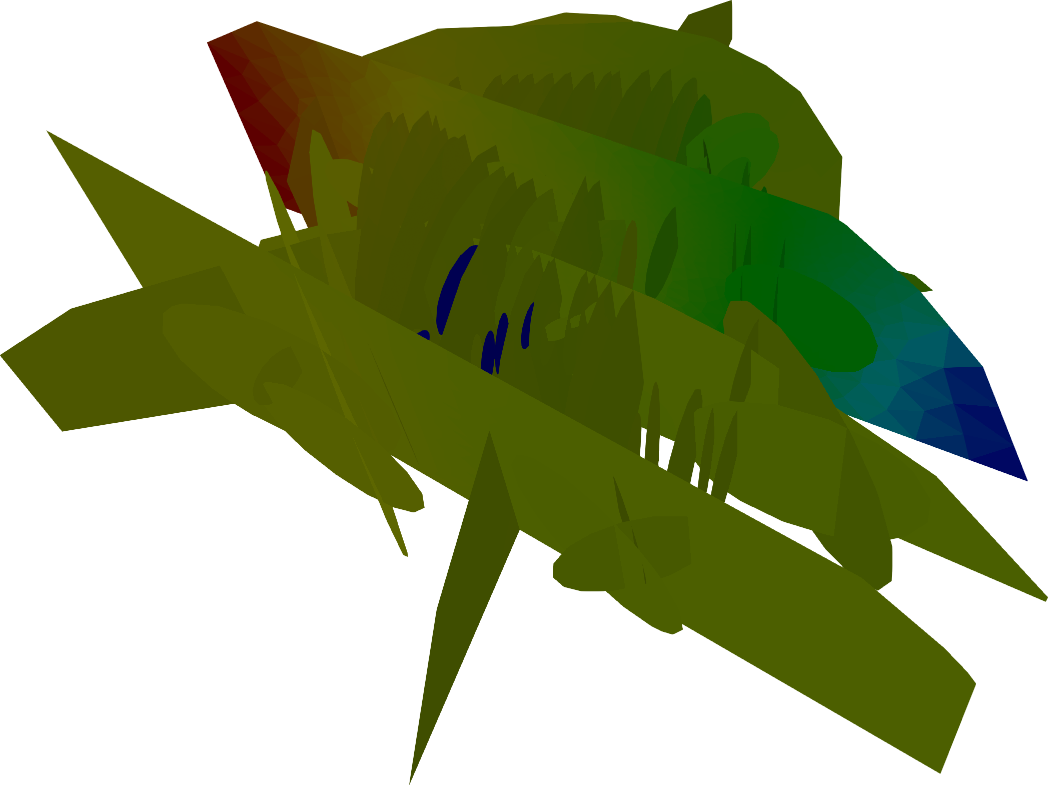
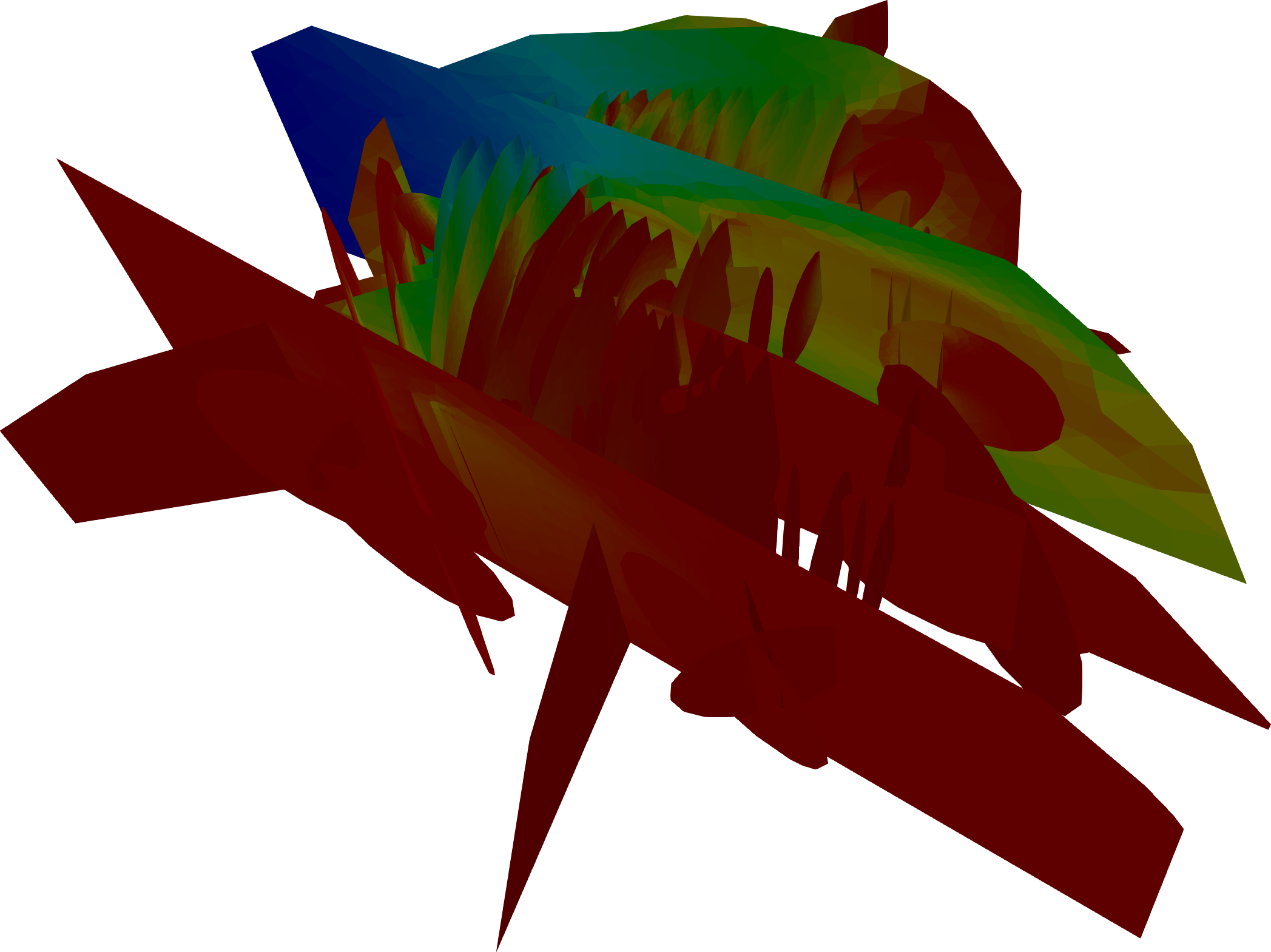
Figure 16: Solution with the mfemup scheme for the Test Case 3: case 1 on the top; case 2 at the bottom. The first column shows the pressure head solution, the second column the temperature distribution at the end of time-evolution.

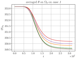
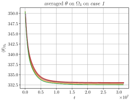
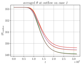
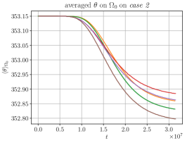
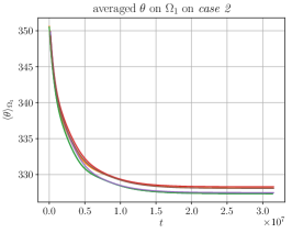
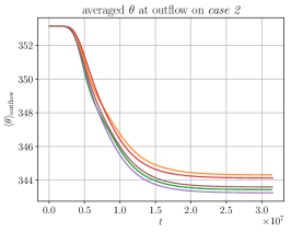
Figure 17: Curves of average theta on fractures $\Omega_{0}$ (left) and $\Omega_{1}$ and at outflow (right) against time for Test Case 3: case 1 top, case 2 bottom.

5 Conclusions

In this work, we presented a detailed comparative study of several solution strategies for single-phase flow and transport in discrete fracture networks. The proposed numerical schemes are challenged with networks of increasing geometrical complexity and with unsteady advection-reaction-diffusion problems. The characteristics of the various approaches are compared in terms of flexibility in handling geometrical complexity, local and global conservativity and stability to high Péclet numbers.

Methods based on matching grids at the traces trade simplicity in imposing coupling conditions with the lack of control on the number of mesh elements, which is actually constrained by the conformity requirement. On the other hand, non-matching and polygonal based approaches demand ad-hoc discretization strategies but allow full flexibility in meshing. Non-locally conservative schemes might be susceptible to loss in mass in particular at the intersection of fractures. The proposed examples showed that this quantity is small and, for many practical problems it is possible to conclude that it might be acceptable compared to the usual uncertainty in the model parameters. Finally, we have compared schemes that are naturally stable with respect to high Péclet number, with schemes that require a stabilization term to avoid spurious oscillations. Also in this case the obtained solutions are coherent with respect to each other. We can conclude that numerical schemes based on polygonal or non-matching meshes give a good balance in terms of computational cost and accuracy with less limitations compared to the matching cases on more standard grids.

References

References

- [1] I. Aavatsmark. Interpretation of a two-point flux stencil for skew parallelogram grids. Computational Geosciences, 11(3):199–206, 2007.
- [2] J. Bear. Dynamics of Fluids in Porous Media. American Elsevier, 1972.
- [3] L. Beirão da Veiga, F. Brezzi, A. Cangiani, G. Manzini, L. D. Marini, and A. Russo. Basic principles of virtual element methods. Mathematical Models and Methods in Applied Sciences, 23(01):199–214, 2013.
- [4] L. Beirão da Veiga, F. Brezzi, L. D. Marini, and A. Russo. H(div) and H(curl)-conforming VEM. Numerische Mathematik, 133(2):303–332, Jun 2014.
- [5] L. Beirão da Veiga, F. Brezzi, L. D. Marini, and A. Russo. The hitchhiker’s guide to the virtual element method. Mathematical Models and Methods in Applied Sciences, 24(08):1541–1573, 2014.
- [6] L. Beirão da Veiga, F. Brezzi, L. D. Marini, and A. Russo. Mixed virtual element methods for general second order elliptic problems on polygonal meshes. ESAIM: Mathematical Modelling and Numerical Analysis, 50(3):727–747, 2016.
- [7] M. F. Benedetto, S. Berrone, A. Borio, S. Pieraccini, and S. Scialò. A hybrid mortar virtual element method for discrete fracture network simulations. Journal of Computational Physics, 306:148 – 166, 2016.
- [8] M. F. Benedetto, S. Berrone, S. Pieraccini, and S. Scialò. The virtual element method for discrete fracture network simulations. Computer Methods in Applied Mechanics and Engineering, 280(0):135–156, 2014.
- [9] M. F. Benedetto, S. Berrone, and S. Scialò. A globally conforming method for solving flow in discrete fracture networks using the virtual element method. Finite Elements in Analysis and Design, 109:23–36, 2016.
- [10] M. Fernando Benedetto, A. Borio, and S. Scialò. Mixed virtual elements for discrete fracture network simulations. Finite Elements in Analysis and Design, 134:55–67, 2017.
- [11] M.F. Benedetto, S. Berrone, A. Borio, S. Pieraccini, and S. Scialò. Order preserving SUPG stabilization for the virtual element formulation of advection-diffusion problems. Computer Methods in Applied Mechanics and Engineering, 311:18–40, 2016.
- [12] S. Berrone and A. Borio. Orthogonal polynomials in badly shaped polygonal elements for the Virtual Element Method. Finite Elements in Analysis and Design, 129:14–31, 2017.
- [13] S. Berrone, A. Borio, and S. Scialò. A posteriori error estimate for a PDE-constrained optimization formulation for the flow in DFNs. SIAM J. Numer. Anal., 54(1):242–261, 2016.
- [14] S. Berrone, A. Borio, and F. Vicini. Reliable a posteriori mesh adaptivity in discrete fracture network flow simulations. Computer Methods in Applied Mechanics and Engineering, 354:904 – 931, 2019.
- [15] S. Berrone, A. D’Auria, and F. Vicini. Fast and robust flow simulations in discrete fracture networks with GPGPUs. GEM - International Journal on Geomathematics, 10(1):8, Jan 2019.
- [16] S. Berrone, S. Pieraccini, and S. Scialò. A PDE-constrained optimization formulation for discrete fracture network flows. SIAM Journal on Scientific Computing, 35(2):B487–B510, 2013.
- [17] S. Berrone, S. Pieraccini, and S. Scialò. On simulations of discrete fracture network flows with an optimization-based extended finite element method. SIAM Journal on Scientific Computing, 35(2):908–935, 2013.
- [18] S. Berrone, S. Pieraccini, and S. Scialò. An optimization approach for large scale simulations of discrete fracture network flows. Journal of Computational Physics, 256:838–853, 2014.
- [19] S. Berrone, S. Pieraccini, and S. Scialò. Towards effective flow simulations in realistic discrete fracture networks. Journal of Computational Physics, 310:181–201, 2016.
- [20] S. Berrone, S. Scialò, and F. Vicini. Parallel meshing, discretization and computation of flow in massive Discrete Fracture Networks. SIAM J. Sci. Comput., 41(4):C317–C338, 2019.
- [21] Stefano Berrone, Sandra Pieraccini, and Stefano Scialò. Flow simulations in porous media with immersed intersecting fractures. Journal of Computational Physics, 345:768 – 791, 2017.
- [22] F. Brezzi, R. S. Falk, and D. L. Marini. Basic principles of mixed virtual element methods. ESAIM: Mathematical Modelling and Numerical Analysis, 48(4):1227–1240, 2014.
- [23] C. D’Angelo and A. Scotti. A mixed finite element method for Darcy flow in fractured porous media with non-matching grids. Mathematical Modelling and Numerical Analysis, 46(02):465–489, 2012.
- [24] P. A. Dowd, J. A. Martin, C. Xu, R. J. Fowell, and K. V. Mardia. A three-dimensional fracture network data set for a block of granite. International Journal of Rock Mechanics and Mining Sciences, 46(5):811–818, 2009.
- [25] J. Erhel, J.-R. de Dreuzy, and B. Poirriez. Flow simulation in three-dimensional discrete fracture networks. SIAM Journal on Scientific Computing, 31(4):2688–2705, 2009.
- [26] B. Flemisch, I. Berre, W. Boon, A. Fumagalli, Nicolas Schwenck, A. Scotti, I. Stefansson, and Alexandru Tatomir. Benchmarks for single-phase flow in fractured porous media. Advances in Water Resources, 111:239–258, Januray 2018.
- [27] L. Formaggia, A. Fumagalli, A. Scotti, and P. Ruffo. A reduced model for Darcy’s problem in networks of fractures. ESAIM: Mathematical Modelling and Numerical Analysis, 48:1089–1116, 7 2014.
- [28] L. P. Franca, S. L. Frey, and T.J.R. Hughes. Stabilized finite element methods: I. Application to the advective-diffusive model. Computer Methods in Applied Mechanics and Engineering, 95(2):253–276, 1992.
- [29] A. Fumagalli. Dual virtual element method in presence of an inclusion. Applied Mathematics Letters, 86:22–29, Dec. 2018.
- [30] A. Fumagalli and E. Keilegavlen. Dual virtual element method for discrete fractures networks. SIAM Journal on Scientific Computing, 40(1):B228–B258, 2018.
- [31] A. Fumagalli and E. Keilegavlen. Dual virtual element methods for discrete fracture matrix models. Oil & Gas Science and Technology - Revue d’IFP Energies nouvelles, 74(41):1–17, 2019.
- [32] A. Fumagalli, E. Keilegavlen, and S. Scialò. Conforming, non-conforming and non-matching discretization couplings in discrete fracture network simulations. Journal of Computational Physics, 376:694–712, 2019.
- [33] A. Fumagalli, E. Keilegavlen, and S. Scialò. Input and benchmarking data for flow simulations in discrete fracture networks. Data in Brief, 21:1135 – 1139, 2018.
- [34] A. Fumagalli and A. Scotti. A numerical method for two-phase flow in fractured porous media with non-matching grids. Advances in Water Resources, 62, Part C(0):454–464, 2013. Computational Methods in Geologic CO2 Sequestration.
- [35] A. Fumagalli and A. Scotti. A reduced model for flow and transport in fractured porous media with non-matching grids, pages 499–507. Springer Berlin Heidelberg, 2013.
- [36] C. Geuzaine and J.-F. Remacle. Gmsh: A 3-d finite element mesh generator with built-in pre- and post-processing facilities. International Journal for Numerical Methods in Engineering, 79(11):1309–1331, 2009.
- [37] N. J. Hardebol, C. Maier, H. Nick, S. Geiger, G. Bertotti, and H. Boro. Multiscale fracture network characterization and impact on flow: A case study on the latemar carbonate platform. Journal of Geophysical Research: Solid Earth, 120(12):8197–8222, 2015. 2015JB011879.
- [38] J. D. Hyman, C. W. Gable, S. L. Painter, and N. Makedonska. Conforming Delaunay Triangulation of Stochastically Generated Three Dimensional Discrete Fracture Networks: A Feature Rejection Algorithm for Meshing Strategy. SIAM Journal on Scientific Computing, 36(4):A1871–A1894, 2014.
- [39] J. D. Hyman, S. Karra, N. Makedonska, C. W. Gable, S. L. Painter, and H. S. Viswanathan. dfnWorks: A discrete fracture network framework for modeling subsurface flow and transport. Computers & Geosciences, 84:10–19, nov 2015.
- [40] E. Keilegavlen, A. Fumagalli, R. Berge, and I. Stefansson. Implementation of mixed-dimensional models for flow in fractured porous media. In Florin Adrian Radu, Kundan Kumar, I. Berre, J. M. Nordbotten, and Iuliu Sorin Pop, editors, Numerical Mathematics and Advanced Applications ENUMATH 2017, volume 126, pages 573–580. Springer International Publishing, 2019.
- [41] E. Keilegavlen, A. Fumagalli, R. Berge, I. Stefansson, and I. Berre. Porepy: An open source simulation tool for flow and transport in deformable fractured rocks. Technical report, arXiv:1712.00460 [cs.CE], 2017.
- [42] V. Martin, J. Jaffré, and J. E. Roberts. Modeling Fractures and Barriers as Interfaces for Flow in Porous Media. SIAM Journal on Scientific Computing, 26(5):1667–1691, 2005.
- [43] M. McClure, M. Babazadeh, S. Shiozawa, and J. Huang. Fully Coupled Hydromechanical Simulation of Hydraulic Fracturing in Three-Dimensional Discrete Fracture Networks. In SPE Hydraulic Fracturing Technology Conference. Society of Petroleum Engineers, feb 2015.
- [44] H. Mustapha and K. Mustapha. A New Approach to Simulating Flow in Discrete Fracture Networks with an Optimized Mesh. SIAM Journal on Scientific Computing, 29(4):1439–1459, 2007.
- [45] T. D. Ngo, A. Fourno, and B. Noetinger. Modeling of transport processes through large-scale discrete fracture networks using conforming meshes and open-source software. Journal of Hydrology, 554:66 – 79, 2017.
- [46] J. M. Nordbotten, W. Boon, A. Fumagalli, and E. Keilegavlen. Unified approach to discretization of flow in fractured porous media. Computational Geosciences, 2018.
- [47] P.-A. Raviart and J.-M. Thomas. A mixed finite element method for second order elliptic problems. Lecture Notes in Mathematics, 606:292–315, 1977.
- [48] J. E. Roberts and J.-M. Thomas. Mixed and hybrid methods. In Handbook of numerical analysis, Vol. II, Handb. Numer. Anal., II, pages 523–639. North-Holland, Amsterdam, 1991.
- [49] J. H. Schön. Physical Properties of Rocks, volume 8 of Handbook of Petroleum Exploration and Production. Elsevier, 2011.
- [50] J. R. Shewchuk. Triangle: Engineering a 2D Quality Mesh Generator and Delaunay Triangulator. In Ming C. Lin and Dinesh Manocha, editors, Applied Computational Geometry: Towards Geometric Engineering, volume 1148 of Lecture Notes in Computer Science, pages 203–222. Springer-Verlag, May 1996. From the First ACM Workshop on Applied Computational Geometry.
- [51] M. Wangen. Physical Principles of Sedimentary Basin Analysis. Cambridge University Press, 2010.