JeLLyFysh-Version1.0 - a Python application for all-atom event-chain Monte Carlo

Abstract

We present JeLLyFysh-Version1.0, an open-source Python application for event-chain Monte Carlo (ECMC), an event-driven irreversible Markov-chain Monte Carlo algorithm for classical $N$-body simulations in statistical mechanics, biophysics and electrochemistry. The application’s architecture closely mirrors the mathematical formulation of ECMC. Local potentials, long-ranged Coulomb interactions and multi-body bending potentials are covered, as well as bounding potentials and cell systems including the cell-veto algorithm. Configuration files illustrate a number of specific implementations for interacting atoms, dipoles, and water molecules.

1 Introduction

Figure 1: ECMC time evolution. At events $E_{a},E_{b},E_{c},\dots$, a number of factors ($\{a_{1},a_{2},\ldots,a_{5}\},\{b_{1},b_{2},\ldots,b_{6}\},\ldots$) are activated. For each leg ($(E_{a}\to E_{b})$, $(E_{b}\to E_{c})$, …), each factor must at all times independently accept the continued non-interacting evolution, and must determine a candidate event time at which this is no longer the case. The earliest candidate event time (which determines the veto) and its out-state yield the next event (the event $E_{b}$ is triggered by $a_{2}$). In JF-V1.0, after committing an event to the global state, candidate events with certain tags are trashed (tags t_1, t_3 at $E_{b}$) or maintained active (tags t_2, t_4 at $E_{b}$), and others are newly activated. JF introduces non-confirmed events and also pseudo-factors, which complement the factors of ECMC, and which may also trigger events.

Event-chain Monte Carlo (ECMC) is an irreversible continuous-time Markov-chain algorithm [5, 28] that often equilibrates faster than its reversible counterparts [30, 19, 22, 23, 24]. ECMC has been successfully applied to the classic $N$-body all-atom problem in statistical physics [4, 17]. The algorithm implements the time evolution of a piecewise non-interacting, deterministic, system [6]. Each straight-line, non-interacting leg of this time evolution terminates in an event, defined through the event time at which it takes place and through the out-state, the updated starting configuration for the ensuing leg. An event is chosen as the earliest of a set of candidate events, each of which is sampled using information contained in a so-called factor. The entire trajectory samples the equilibrium probability distribution.

ECMC departs from virtually all Monte Carlo methods in that it does not evaluate the equilibrium probability density (or its ratios). In statistical physics, ECMC thus computes neither the total potential (or its changes) nor the total force on individual point masses. Rather, the decision to continue on the current leg of the non-interacting time evolution builds on a consensus which is established through the factorized Metropolis algorithm [28]. A veto puts an end to the consensus, triggers the event, and terminates the leg (see Fig. 1). In the continuous problems for which ECMC has been conceived, the veto is caused by a single factor.

The resulting event-driven ECMC algorithm is reminiscent of molecular dynamics, and in particular of event-driven molecular dynamics [1, 2, 3], in that there are velocity vectors (which appear as lifting variables). These velocities do not correspond to the physical (Newtonian) dynamics of the system. ECMC differs from molecular dynamics in three respects: First, ECMC is event-driven, and it remains approximation-free, for any interaction potential [32], whereas event-driven molecular dynamics is restricted to hard-sphere or piecewise constant potentials. (Interaction potentials in biophysical simulation codes have been coarsely discretized [8] in order to fit into the event-driven framework [36, 33, 34].) Second, in ECMC, most point masses are at rest at any time, whereas in molecular dynamics, all point masses typically have non-zero velocities. In ECMC, an arbitrary fixed number of (independently) active point masses (with non-zero velocities) and identical velocity vectors for all of them may be chosen. In JF-V1.0, as in most previous applications of ECMC, only a single independent point mass is active. The ECMC dynamics is thus very simple, yet it mixes and relaxes at a rate at least as fast as in molecular dynamics [19, 23, 24]. Third, ECMC by construction exactly samples the Boltzmann (canonical) distribution, whereas molecular dynamics is in principle micro-canonical, that is, energy-conserving. Molecular dynamics is thus generally coupled to a thermostat in order to yield the Boltzmann distribution. The thermostat there also eliminates drift in physical observables due to integration errors. ECMC is free from truncation and discretization errors.

ECMC samples the equilibrium Boltzmann distribution without being itself in equilibrium, as it violates the detailed-balance condition. Remarkably, it establishes the aforementioned consensus and proceeds from one event to the next with $\mathcal{O}(1)$ computational effort even for long-range potentials, as was demonstrated for soft-sphere models, the Coulomb plasma [18, 19], and for the simple point-charge with flexible water molecules (SPC/Fw) model [39, 9].

JeLLyFysh (JF) is a general-purpose Python application that implements ECMC for a wide range of physical systems, from point masses interacting with central potentials to composite point objects such as finite-size dipoles, water molecules, and eventually peptides and polymers. The application’s architecture closely mirrors the mathematical formulation that was presented previously (see [9, Sect II]). The application can run on virtually any computer, but it also allows for multiprocessing and, in the future, for parallel implementations. It is being developed as an open-source project on GitHub. Source code may be forked, modified, and then merged back into the project (see Section 6 for access information and licence issues). Contributions to the application are encouraged.

The present paper introduces the general architecture and the key features of JF. It accompanies the first public release of the application, JeLLyFysh-Version1.0 (JF-V1.0). JF-V1.0 implements ECMC for homogeneous, translation-invariant $N$-body systems in a regularly shaped periodic simulation box and with interactions that can be long-ranged. In addition, the present paper presents a cookbook that illustrates the application for simplified core examples that can be run from configuration files and validated against published data [9]. A full-scale simulation benchmark against the Lammps application is published elsewhere [35].

The JF application presented in this paper is intended to grow into a basis code that will foster the development of irreversible Markov-chain algorithms and will apply to a wide range of computational problems, from statistical physics to field theory [13]. It may prove useful in domains that have traditionally been reserved to molecular dynamics, and in particular in the all-atom Coulomb problem in biophysics and electrochemistry.

The content of the present paper is as follows: The remainder of Section 1 discusses the general setting of JF as it implements ECMC. Section 2 describes its mediator-based architecture [10]. Section 3 discusses how the eponymous events of ECMC are determined in the event handlers of JF. Section 4 presents system definitions and tools, such as the user interface realized through configuration files, the simulation box, the cell systems, and the interaction potentials. Section 5, the cookbook, discusses a number of worked-out examples for previously presented systems of atoms, dipoles or water molecules with Coulomb interactions [9]. Section 6 discusses licence issues, code availability and code specifications. Section 7 presents an outlook on essential challenges and a preview of future releases of the application.

1.1 Configurations, factors, pseudo-factors, events, event handlers

In ECMC, configurations $c=\{\mathbf{s}_{1},\ldots,\mathbf{s}_{i},\ldots,\mathbf{s}_{N}\}$ are described by continuous time-dependent variables where $\mathbf{s}_{i}(t)$ represents the position of the $i$th of $N$ point masses (although it may also stand for the continuous angle of a spin on a lattice [30]). JF is an event-driven implementation of ECMC, and it treats point masses and certain collective variables (such as the barycenter of a composite point object) on an equal footing. Rather than the time-dependent variables $\mathbf{s}_{i}(t)$, its fundamental particles ( Particle objects) are individually time-sliced positions (of the point masses or composite point objects). Non-zero velocities and time stamps are also recorded, when applicable. The full information can be packed into units ( Unit objects), that are moved around the application (see Section 1.2).

Each configuration $c$ has a total potential $U(\{\mathbf{s}_{1},\ldots,\mathbf{s}_{N}\})$, and its equilibrium probability density $\pi$ is given by the Boltzmann weight

$$\pi(\{\mathbf{s}_{1},\ldots,\mathbf{s}_{N}\})=\exp\left[-\beta U(\{\mathbf{s}_{1},\ldots,\mathbf{s}_{N}\})\right],$$ (1)

that is sampled by ECMC (see [9]). The total potential $U$ is decomposed as

$$U(\{\mathbf{s}_{1},\ldots,\mathbf{s}_{N}\})=\sum_{M\in\mathcal{M}}U_{M}(\{\mathbf{s}_{i}:i\in I_{M}\}),$$ (2)

and the Boltzmann weight of eq. (1) is written as a product over terms that depend on factors $M$, with their corresponding factor potentials $U_{M}$. A factor $M=(I_{M},T_{M})$ consists of an index set $I_{M}$ and of a factor type $T_{M}$, and $\mathcal{M}$ is the set of factors that have a non-zero contribution to eq. (2) for some configuration $c$. In the SPC/Fw water model, for example, one factor $M$ with factor type $T_{M}=\text{Coulomb}$ might describe all the Coulomb potentials between two given water molecules, and the factor index set $I_{M}$ would contain the identifiers (indices) of the involved four hydrogens and two oxygens (see Section 5.3).

ECMC relies on the factorized Metropolis algorithm [28], where the move from a configuration $c$ to another one, $c^{\prime}$, is accepted with probability

$$p^{\text{Fact}}(c\to c^{\prime})=\prod_{M}\min\left[1,\exp\left(-\beta\Delta U_{M}\right)\right],$$ (3)

where $\Delta U_{M}=U_{M}(c^{\prime}_{M})-U_{M}(c_{M})$. Rather than to evaluate the right-hand side of eq. (3), the product over the factors is interpreted as corresponding to a conjunction of independent Boolean random variables

$$X^{\text{Fact}}(c\to c^{\prime})=\bigwedge_{M\in\mathcal{M}}X_{M}(c_{M}\to c^{\prime}_{M}).$$ (4)

In this equation, $X^{\text{Fact}}(c\to c^{\prime})$ is “True” (the proposed Monte Carlo move is accepted) if the independently sampled factorwise Booleans $X_{M}$ are all “True”. Equivalently, the move $c\to c^{\prime}$ is accepted if it is independently accepted by all factors. This realizes the aforementioned consensus decision (see Fig. 1). For an infinitesimal displacement, the random variable $X_{M}$ of only a single factor $M$ can be “False”, and the factor $M$ vetoes the consensus, creates an event, and starts a new leg. In this process, $M$ requires only the knowledge of the factor in-state (based on the configuration $c_{M}$, and the information on the move), and the factor out-state (based on $c^{\prime}_{M}$) provides all information on the evolution of the system after the event. The event is needed in order to enforce the global-balance condition (see Fig. 2a). In this process, lifting variables [7], corresponding to generalized velocities, allow one to repeat moves of the same type (same particle, same displacement), as long as they are accepted by consensus. Physical and lifting variables build the overcomplete description of the Boltzmann distribution at the base of ECMC, and they correspond to the global physical and global lifting states of JF, its global state.

Figure 2: Factors and pseudo-factors. (a): In-state and sampled out-state (each with two active units) for a three-unit factor $M$ (implementing, for example, the inter-molecular bending potential $U_{M}$ of Section 4.4.5). (b): In- and out-states for a cell-boundary event handler realizing a pseudo-factor. Times at which units are time-sliced are indicated. $t_{\text{out}}$ is the event time.

JF, the computer application, is entirely formulated in terms of events, beyond the requirements of the implemented event-driven ECMC algorithm. The application relies on the concept of pseudo-factors, which complement the factors in eq. (2), but are independent of potentials and without incidence on the global-balance condition (see Fig. 2b). In JF, the sampling of configuration space, for example, is expressed through events triggered by pseudo-factors. Pseudo-factors also trigger events that interrupt one continuous motion (one “event chain” [5]) and start a new one. Even the start and the end of each run of the application are formulated as events triggered by pseudo-factors.

In ECMC, among all factors $M$ in eq. (2), only those for which $U_{M}$ changes along one leg can trigger events. In JF, these factors are identified in a separate element of the application, the activator (see Section 2.4), and they are realized in yet other elements, the event handlers. An event handlers may require an in-state. It then computes the candidate event time and its out-state (from the in-state, from the factor potential, and from random elements). The complex operation of the activator and the event handlers is organized in JF-V1.0 with the help of a tag activator, with tags essentially providing finer distinction than the factor types $T_{M}$. A tagger identifies a certain pool of factors, and also singles out factors that are to be activated for each tag. The triggering of an event associated with a given tag entails the trashing of candidate events with certain tags, while other candidate events are maintained (see Fig. 1). Also, new candidate events have to be computed by event handlers with given tags. This entire process is managed by the tag activator.

1.2 Global state, internal state

In the event-driven formulation of ECMC, a point mass with identifier $\sigma$ and with zero velocity is simply represented through its position, while an active point mass (with non-zero velocity) is represented through a time-sliced position $\mathbf{s}_{\sigma}(t_{\sigma})$, a time stamp $\sigma(t_{\sigma})$ and a velocity $\mathbf{v}_{\sigma}$:

$$\mathbf{s}_{\sigma}(t)=\begin{cases}\mathbf{s}_{\sigma}&\quad\text{if $\mathbf{v}_{\sigma}=0$}\\ \mathbf{s}_{\sigma}(t_{\sigma})+(t-t_{\sigma})\mathbf{v}_{\sigma}&\quad\text{else (active point mass)}\end{cases}.$$ (5)

An active point mass thus requires storing of a velocity $\mathbf{v}_{i}$ and of a time stamp $t_{\sigma}$, in addition to the time-sliced position $\mathbf{s}_{\sigma}(t_{\sigma})$. In JF, the global state traces all the information in eq. (5). It is broken up into the global physical state, for the time-sliced positions $\mathbf{s}_{\sigma}$, and the global lifting state, for the non-zero velocities $\mathbf{v}_{\sigma}$ and the time stamps $t_{\sigma}$.

JF represents composite point objects as trees described by nodes. Leaf nodes correspond to the individual point masses. A tree’s inner nodes may represent, for example, the barycenters of parts of a molecule, and the root node that of the entire molecule (see Fig. 3a-b). The velocities inside a composite point object are kept consistent, which means that the global lifting state includes non-zero velocities and time stamps of inner and root nodes. The storing element of the global state in JF is the state handler (see Section 2.3). The global state is not directly accessed by other elements of the application, but branches of the tree can be extracted (copied) temporarily, together with their unit information. Independent and induced units differentiate between those that appear in ECMC and those that are carried along in order to assure consistency (see Fig. 3).

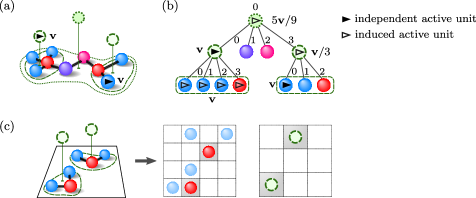
Figure 3: Tree representation of composite point objects in JF-V1.0. (a): Molecule with functional parts. (b): Tree representation, with leaf nodes for the individual atoms and higher-level nodes for barycenters. Nodes each have a particle (a Particle object) containing a position vector and charge values. A unit (a Unit object), associated with a node, copies out the particle’s identifier and its complete global-state information. (c): Internal representation of composite point objects with separate cell systems for particle identifiers on different levels. On the leaf level, only one kind of particles is tracked.

For internal computations, the global state may be supplemented by an internal state that is kept, not in the state handler, but in the activator part of the application (see Section 2.4). In JF-V1.0, the internal state consists in cell-occupancy systems, which associate identifiers of composite point objects or point masses to cells. (An identifier is a generalized particle index with, in the case of a tree, a number of elements that correspond to the level of the corresponding node.) In JF, cell-occupancy systems are used for book-keeping, and also for cell-based bounding potentials. JF-V1.0 requires consistency between the time-sliced particle information and the units. This means that the time-sliced position $\mathbf{s}_{\sigma}(t_{\sigma})$ and the time-dependent position $\mathbf{s}_{\sigma}(t)$ in eq. (5) belong to the same cell (see Fig. 2b). Several cell-occupancy systems may coexist within the internal state (possibly on different tree-levels and with different cell systems, see Fig. 3c and Section 5.3.4). ECMC requires time-slicing only for units whose velocities are modified. Beyond the consistency requirements, JF-V1.0 performs time-slicing also for unconfirmed events, that is, for triggered events for which, after all, the out-state continues the straight-line motion of the in-state (see Section 3.1.2).

1.3 Lifting schemes

In its lifted representation of the Boltzmann distribution, ECMC introduces velocities for which there are many choices, that is, lifting schemes. The number of independent active units can in particular be set to any value $n_{\text{ac}}>1$ and then held fixed throughout a given run. This generalizes easily from the known $n_{\text{ac}}=1$ case [12]. A simple $n_{\text{ac}}$-conserving lifting scheme uses a factor-derivative table (see [9, Fig. 2]), but confirms the active out-state unit only if the corresponding unit is not active in the in-state (its velocity is None). For $|I_{M}|>3$, the lifting scheme (the way of determining the out-state given the in-state) is not unique, and its choice influences the ECMC dynamics [9]. In JF-V1.0, different lifting-scheme classes are provided in the JF  lifting package. They all construct independent-unit out-state velocities for independent units that equal the in-state velocities. This appears as the most natural choice in spatially homogeneous systems [5].

1.4 Multiprocessing

In ECMC, factors are statistically independent. In JF, therefore, the event handlers that realize these factors can be run independently on a multiprocessor machine. With multiprocessor support enabled, candidate events are concurrently determined by event handlers on separate processes, using the Python multiprocessing module. Candidate event times are then first requested in parallel from active event handlers, and then the out-state for the selected event. Given a sufficient number of available processors, out-states may be computed for candidate events in advance, before they are requested (see Section 2.1). The event handlers themselves correspond to processes that usually last for the entire duration of one ECMC run. When not computing, event handlers are either in idle stage waiting to compute an candidate event time or in suspended stage waiting to compute an out-state.

Using multiple processes instead of threads circumvents the Python global interpreter lock, but the incompressible time lag due to data exchange slows down the multiprocessor implementation of the mediator with respect to the single-processor implementation.

1.5 Parallelization

ECMC generalizes to more than one independent active unit, and a sequential, single-process ECMC computation remains trivially correct for arbitrary $n_{\text{ac}}$ (although JF-V1.0 only fully implements the $n_{\text{ac}}=1$ case). The relative independence of a small number of independent active units in a large system, for $1\ll n_{\text{ac}}\ll N$, allows one to consider the simultaneous committing in different processes of $n_{\text{pr}}$ events to the shared global state. (A conflict arises if this disagrees with what would result by committing them in a single process.) If $n_{\text{pr}}\ll N$, conflicts between processes disappear (for short-range interacting systems) if nearby active units are treated in a single process (see Fig. 4a). The parallel implementation of ECMC, for short-range interactions, is conceptually much simpler than that of event-driven molecular dynamics [29, 14, 20], and it may well extend to long-range interacting system.

An alternative type of parallel ECMC, domain decomposition into $n_{\text{ac}}$ stripes, was demonstrated for two-dimensional hard-spheres systems, and considerable speed-up was reached [16]. Here, stripes are oriented parallel to the velocities, with one active unit per stripe. Stripes are isolated from each other by immobile layers of spheres [16], which however cause rejections (or reversals of one or more components of the velocity). The stripe decomposition eliminates all scheduling conflicts. As any domain decomposition [29], it is restricted to physical models with short-range interactions. It is not implemented in JF-V1.0 (see Fig. 4b).

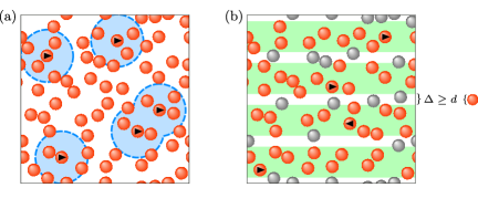
Figure 4: Parallel ECMC with local potentials (interaction range $d$). (a): Multiprocess version with $n_{\text{ac}}\ll N$ active units. Nearby active units avoid conflict in a single process. (b): Domain decomposition with separated stripes. Particles in between stripes are immobile. The separation region (of width $\Delta$) is wider than $d$, so that all conflict between stripes is avoided (see [16]).

2 JF architecture

JF adopts the design pattern based on a mediator [10], which serves as the central hub for the other elements that do not directly connect to each other. In this way, interfaces and data exchange are particularly simple. The mediator design maximizes modularity in view of future extensions of the application.

2.1 Mediator

The mediator is doubled up into two modules (with SingleProcessMediator and MultiProcessMediator classes). The run method of either class is called by the executable run.py script of the application, and it loops over the legs of the continuous-time evolution. The loop is interrupted when an EndOfRun exception is raised, and a post_run method is invoked. For the single-process mediator, all the other elements are instances of classes that provide public methods. In particular, the mediator interacts with event handlers. For the multi-process mediator, each event handler has its own autonomous iteration loop and runs in a separate process. It exchanges data with the mediator through a two-way pipe. Receiving ends on both sides detect when data is available using the pipe’s recv methods.

In JF-V1.0, the same event-handler classes are used for the single-process and multi-process mediator classes. The multi-process mediator achieves this through a monkey-patching technique. It dynamically adds a run_in_process method to each created instance of an event handler, which then runs as an autonomous iteration loop in a process and reacts to shared flags set by the mediator. The multi-process mediator in addition decorates the event handler’s send_event_time and send_out_state methods so that output is not simply returned (as it is in the single-process mediator) but rather transmitted through a pipe. Only the mediator accesses the event handlers, and these re-definitions of methods and classes (which abolish the need for two versions for each event-handler class) are certain not to produce undesired side effects.

On one leg of the continuous-time evolution, the mediator goes through nine steps (see Fig. 5). In step $1$, the active global state (that part of the global state that appears in the global lifting state) is obtained from the state handler. (In the tree state handler of JF-V1.0, branches of independent units are created for all identifiers that appear in the lifting state.) Knowing the preceding event handler (which initially is None) and the active global state, it then obtains from the activator, in step $2$, the event handlers to activate together with their in-state identifiers. For this, the activator may rely on its internal state, but not on the global state, to which it has no access. In step $3$, the corresponding in-states are extracted (that is, copied) from the state handler. In step $4$, candidate event times are requested from the appropriate event handlers and pushed into the scheduler’s push_event method. In step $5$, the mediator obtains the earliest candidate event time from the scheduler’s get_succeeding_event method and and asks its event handler for the event out-state (step $6$) to be committed to the global state (step $7$). The activator, in step $8$, determines which candidate events are to be trashed (in JF-V1.0: based on their tags), that is, which candidate event times are to be eliminated from the scheduler. Also, the activator collects the corresponding event handlers, as they become available to determine new candidate events. In the optional final step $9$, the mediator may connect (via the input–output handler) to an output handler, depending on the preceding event handler. A mediating method defines the arguments sent to the output handler (for example the extracted global state), and considerable computations may take place there.

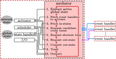
Figure 5: JF architecture, built on the mediator design pattern. The iteration loop takes the system from one event to the next (for example from $E_{a}$ to $E_{b}$ in Fig. 1). All elements of JF interact with the mediator, but not with each other. The multi-process mediator interacts with event handlers running on separate processes, and exchanges data via pipes.

The multi-process mediator uses a single pipe to receive the candidate event time and the out-state from an event handler. In order to distinguish the received object, the mediator assigns four different stages to the event handlers ( idle, event_time_started, suspended, out_state_started stages). The assigned stage determines which flags can be set to start the send_event_time or send_out_state methods. It also determines the nature of the data contained in the pipe. In the idle stage, the mediator can set the starting flag after which the event handler will wait to receive the in-state through the pipe. This starts the event_time_started stage during which the event handler determines the next candidate event time and places it into the pipe. After the mediator has recovered the data from the pipe, it places the event handler into the suspended stage. If requested (by flags), the event handler can then either compute the out-state ( out_state_started stage), or else revert to the event_time_started stage.

The strategy for suspending an event handler or for having it start an out-state computation (before the request) can be adjusted to the availability of physical processors on the multi-processor machine. However, in JF-V1.0, the communication via pipes presents a computational bottleneck.

2.2 Event handlers

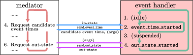
Figure 6: Basic stages of event handlers for factors and pseudo-factors (stages 1 and 3 relevant for the multi-process mediator only). In the idle and suspended stages, the event handler is halted (via flags controlled by the multi-process mediator), thus liberating resources for other candidate-event-time requests. With the multi-process mediator, candidate out-states may be computed before the out-state request arrives.

Event handlers (instances of a number of classes that inherit from the abstract EventHandler class) provide the send_event_time and send_out_state methods that return candidate events. These candidate events either become events of a factor or pseudo-factor or they will be be trashed.

When realizing a factor or a pseudo-factor, event handlers receive the in-state as an argument of the send_event_time method. The send_out_state method then takes no argument. In contrast, event handlers that realize a set of factors or pseudo-factors request candidate event times without first specifying the complete in-state, because the element of the set that triggers the event is yet unknown at the event-time request (see Section 3.2.2 for examples of event handlers that realize sets of factors). The send_event_time method then takes the part of the in-state which is necessary to calculate the candidate event time. Also, it may return supplementary arguments together with the candidate event time, which is used by the mediator to construct the full in-state. The in-state is then an argument of the send_out_state method, as it was not sent earlier.

In JF-V1.0, each run requires a start-of-run event handler (an instance of a class that inherits from the abstract StartOfRunEventHandler class), and it cannot terminate properly without an end-of-run event handler. Section 3 discusses several event-handler classes that are provided.

2.3 State handler

The state handler (an instance of a class that inherits from the abstract StateHandler class) is the sole separate element of JF to access the global state. In JF-V1.0, the global physical state (all positions of point masses and composite point objects) is contained in an instance of the TreePhysicalState class represented as a tree consisting of nodes (each node corresponds to a Node object). Each node contains a particle (a Particle object) which holds a time-sliced position. In JF-V1.0, each leaf node may in addition have charges as a Python dictionary mapping the name of the charge onto its value.

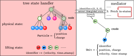
Figure 7: Inner storage of the tree state handler and example of its extract_from_global_state method, applied to the global state of Fig. 3b.

Each tree is specified through its root node. Root nodes can be iterated over (in JF-V1.0, they are members of a list). Each node is connected to its parent and its children, which can also be iterated over. In JF-V1.0, the children are again members of a list. These lists imply unique identifiers of nodes and their particles as tuples. The first entry of the tuple gives a node’s root node list index, followed by the indices on lower levels down to the node itself (see Fig. 3).

The global lifting state is stored in JF-V1.0 in a Python dictionary mapping the implicit particle identifier onto its time stamp and its velocity vector. This information is contained in an instance of the TreeLiftingState class. Both the physical and lifting states are combined in the TreeStateHandler which implements all methods of a state handler.

To communicate with other elements of the JF application (such as the event handlers and the activator) via the mediator, the state handler combines the information of the global physical and the global lifting state into units (that is, temporary Unit objects, see Fig. 7). A given physical-state and lifting-state information for a node in the state handler is mirrored (that is copied) to a unit containing its implicit identifier, position, charge, velocity and time stamp. All other elements can access, modify, and return units. This provides a common packaging format across JF. The explicit identifier of a unit allows the program to integrate changed units into the state handler’s global state.

In the tree state handler of JF-V1.0, the local tree structure of nodes can be extracted into a branch of cnodes, that is, nodes containing units. Each event handler only requires the global state reduced to a single factor in order to determine candidate event times and out-states. As a design principle in JF-V1.0, the event handlers keep the time-slicing of composite point objects and its point masses consistent. Information sent to event handlers via the mediator is therefore structured as branches, that is the information of a node with its ancestors and descendants. The state handler’s extract_from_global_state method creates a branch for a given identifier of a particle by constructing a temporary copy of the immutable node structure of the state handler using cnodes. Out-states of events in the form of branches can be committed to the global state using the insert_into_global_state method.

The extract_active_global_state method, the first of two additional methods provided by the state handler, extracts the part of the global state which appears in the global lifting state. The tree state handler constructs the minimal number of branches, where each node contains an active unit, so that all implicit identifiers appearing in the global lifting state are represented. The activator may then determine the factors which are to be activated. The method is also used to time-slice the entire global state (see Section 3.2.2). Second, the extract_global_state method extracts the full global state. (For the tree state handler of JF-V1.0, this corresponds to a branch for each root node.) This method does not copy the positions and velocities.

In JF-V1.0, the global physical state is initialized via the input handler within the input–output handler (see Section 2.6). The initial lifting state, however, is set via the out-state of the start-of-run event handler, which is committed to the global state at the beginning of the program (see Section 3.2.2). This means that, in JF-V1.0, the lifting state cannot be initialized from a file.

2.4 Activator

The activator, a separate element of the JF application, is an instance of a class that inherits from the abstract Activator class. At the beginning of each leg, the activator provides to the mediator the new event handlers which are to be run, using the get_event_handlers_to_run method. (As required by the mediator design pattern, no data flows directly between the activator and the event handlers, although it initially obtains their references, and subsequently manages them.) The activator also returns associated in-state identifiers of particles within the global state. The extracted parts of the global state of these are needed by the event handlers to compute their candidate event time (the identifier may be None if no information is needed). Finally, it readies for the mediator a list of trashable candidate events at the end of each leg in the get_trashable_events method, once the mediator has committed the preceding event to the global state via the state handler.

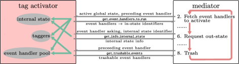
Figure 8: Tag activator, and its complex interaction with the mediator. It readies event handlers and in-state identifiers, provides internal-state information for an out-state request, and identifies the trashable candidate events, as a function of the preceding event.

In JF-V1.0, the activator is an instance of the TagActivator class (that inherits from the Activator class). The tag activator’s operations depend on the interdependence of tags of event handlers and their events. Event handlers receive their tag by instances of classes located in the activator and derived from the abstract Tagger class that are called “taggers”.

A tagger centralizes common operations for identically tagged event handlers (see Fig. 8). On initialization, the tagger receives its tag (a string-valued tag attribute) and an event handler (that is, a single instance), of which it creates as many identical event-handler copies as needed (using the Python deepcopy method). Each tagger provides a yield_identifiers_send_event_time method which generates in-state identifiers based on the branches containing independent active units (this means that the taggers are implemented especially for the TreeStateHandler, the TagActivator however is not restricted to this since it just transmits the extracted active global state). These in-states are passed (after extracting the part of the global state related to the identifiers from the state handler) to the send_event_time method of the tagger’s event handlers. The number of event handlers inside a tagger should meet the maximum number of events with the given tag simultaneously in the scheduler. In this paper, event handlers (and their candidate events) are referred to by tags, although in JF they do not have the tag attribute of their taggers.

On initialization, a tagger also receives a list of tags for event handlers that it creates, as well as a list of tags for event handlers that need to be trashed. The tag activator converts this information of all taggers into its internal _create_taggers and _trash_taggers dictionaries. Additionally, the tag activator creates an internal dictionary mapping from an event handler onto the corresponding tagger (_event_handler_tagger_dictionary).

A call of the get_event_handlers_to_run method is accompanied by the event handler which created the preceding event and by the extracted active global state. The event handler is first mapped onto its tagger. The taggers returned by the _create_taggers dictionary then generate the in-states identifiers, which are returned together with the corresponding event handlers (in a dictionary). For the initial call of the get_event_handlers_to_run method no information on the preceding event handler can be provided. This is solved by initially returning the start-of-run event handler. Similarly the _trash_taggers dictionary is used on each call of get_trashable_events. The corresponding event handlers are then also liberated, meaning that the activator can return them in the next call of the get_event_handlers_to_run method. For this, the activator internally splits the pool of all event handlers of a given tag internally into those with a scheduled candidate event and the ones that are available to take on new candidate events.

The activator also maintains the internal state. In JF-V1.0, the internal state consists in cell-occupancy systems. Therefore, the internal state is an instance of a class that inherits from the CellOccupancy class, which itself inherits from the abstract InternalState class. Taggers may refer to internal-state information to determine the in-states of their event handlers. The cell-occupancy system does not double up on the information available in the state handler. It keeps track of the identifier of a particle (which may correspond to a point mass or a composite point object), but does not store or copy the particle itself (see Section 4.3). The mediator can access the internal state via the get_info_internal_state method (see Fig. 8). To acquire consistency between the global state and the internal state (and between a particle and its associated unit), a pseudo-factor triggers an event for each active unit tracked by the cell-occupancy system that crosses a cell boundary (see Fig. 2b). The internal state is updated in each call of the get_event_handlers_to_run method.

2.5 Scheduler

The scheduler is an instance of a class inheriting from the abstract Scheduler class. It keeps track of the candidate events and their associated event-handler references. Its get_succeeding_event method selects among the candidate events the one with the smallest candidate event time, and it returns the reference of the corresponding event handler. Its push_event method receives a new candidate event time and event-handler reference. Its trash_event method eliminates a candidate event, based on the reference of its event handler. In JF-V1.0, the scheduler is an instance of the HeapScheduler class. It implements a priority queue through the Python heapq module.

2.6 Input–output handler

The input–output handler is an instance of the InputOutputHandler class. The input–output handler connects the JF application to the outside world, and it is accessible by the mediator. The input–output handler breaks up into one input handler (an instance of a class that inherits from the abstract InputHandler class) and a possibly empty list of output handlers (instances of classes that inherit from the abstract OutputHandler class). These are accessed by the mediator only via the input–output handler. Output handlers can also perform significant calculations.

The input handler enters the initial global physical state into the application. JF-V1.0 provides an input handler that enters protein-data-bank formatted data (.pdb files) as well as an input handler which samples a random initial state. The initial state (constructed as a tree for the case of the tree state handler) is returned when calling the read method of the input–output handler, which calls the read method of the input handler.

The output handlers serve many purposes, from the output in .pdb files to the sampling of correlation functions and other observables, to a dump of the entire run. They obtain their arguments (for example the entire global state) via its write method. The write method of the input–output handler receives the desired output handler as an additional argument through the mediating methods of specific event handlers. These are triggered for example after a sampling or an end-of-run event. The corresponding event handlers are initialized with the name of their output handlers.

3 JF event-handler classes

Event handler classes differ in how they provide the send_event_time and send_out_state methods. Event handlers split into those that realize factors and sets of factors and those that realize pseudo-factors and sets of pseudo-factors. The first are required by ECMC while the second permit JF to represent the entire run in terms of events.

3.1 Event handlers for factors or sets of factors

Event handlers that realize a factor $M$, or a set of factors are implemented in different ways depending on the analytic properties of the factor potential $U_{M}$ and on the number of independent active units.

3.1.1 Invertible-potential event handlers

In JF, an invertible factor potential $U_{M}$ (an instance of a class that inherits from the abstract InvertiblePotential class) has its event rate integrated in closed form along a straight-line trajectory (see Fig. 1). The sampled cumulative event rate ($U_{M}^{+}$ in [9, eq. (45)]) provides the displacement method. Together with the time stamp and the velocity of the active unit, this determines the candidate event time. In JF-V1.0, the two-leaf-unit event handler (an instance of the TwoLeafUnitEventHandler class) is characterized by two independent units at the leaf level. It realizes a two-particle factor with an invertible factor potential. The in-state (an argument of the send_event_time method) is stored internally, and it remains available for the subsequent call of the send_out_state method. Because of the two independent units, the lifting simply consists in these two units switching their velocities (using the internal _exchange_velocity method) and keeping the velocities of all induced units consistent.

3.1.2 Event handlers for factors with bounding potential

For a factor potential $U_{M}$ that is not inverted (by choice or by necessity because it is non-invertible), the cumulative event rate $U_{M}^{+}$ is unavailable (or not used) and so is its displacement method. Only the derivative method is used. To realize such a factor without an inverted factor potential, an event handler then uses the displacement method of an associated bounding potential whose event rate at least equals that of $U_{M}$ and that is itself invertible. A non-inverted $U_{M}$ may be associated with more than one bounding potential, each corresponding to a different event handler (the molecular Coulomb factors in Section 5.2 associate the Coulomb factor potential in the same run with different bounding potentials). In JF-V1.0, a number of event handlers are instances of classes that inherit from the EventHandlerWithBoundingPotential class, and that realize factors with bounding potentials. Each of these event handlers translates the sampled displacement of the bounding potential into a candidate event time. On an out-state request (via the send_out_state method), the event handler confirms the event with probability that is given by the ratio of the event rates of the factor potential and the bounding potential. The out-state consists of independent units together with their branches of induced units. For two independent units, the lifting limits itself to the application of a local _exchange_velocity method, which exchanges independent-unit velocities and enforces velocities for the induced units. For more independent units, the out-state calculation requires a lifting. For an unconfirmed event, no lifting takes place. In JF-V1.0, confirmed and unconfirmed event have time-sliced out-states. Inefficient treatment of unconfirmed events is the main limitation of this version of the application.

A special case of a bounding potential is the cell-based bounding potential which features piecewise cell-bounded event rates. The two independent units are localized within their respective cells, and the bounding potential’s rate is for all positions of the units larger than the factor potential event rate. In JF-V1.0, the constant cell-bounded event rate is determined for all pairs of cells on initialization (see Section 4.4.4). The resulting displacement may move the independent active unit outside its cell. The proposed candidate event will then however be preempted by a cell-boundary event and then trashed (see Section 3.2.1).

3.1.3 Cell-veto event handlers

Cell-veto event handlers (instances of a number of classes that inherit from the abstract CellVetoEventHandler class) realize sets of factors, rather than a single factor. The factor in-states (for each element of the set) are not transmitted with the candidate-event-time request. Instead, the branch of the independent active unit is an argument of the send_event_time method. The sampled factor in-state is transmitted with the out-state request. The cell-veto event handler implements Walker’s algorithm [37] in order to sample one element in the set of factors in $\mathcal{O}(1)$ operations.

Cell-veto event handlers are instantiated with an estimator (see Section 4.6). In addition, they obtain a cell system which is read in through its initialize method (see Section 4.2). The estimator provides upper limits for the event rate (in the given direction of motion) for the independent active unit anywhere in one specific cell (called “zero-cell”, see Section 4.3), and for a target unit in any other cell, except for a list of excluded cells. These upper limits can be translated from the zero-cell to any other active-unit cell, because of the homogeneity of the simulation box. In JF-V1.0, the cell systems for the cell-veto event handler can be on any level of the particles’ tree representation (see Section 5.3.4, where a molecule-cell system tracks individual water molecules on the root level, while a oxygen-cell system tracks only the leaf nodes corresponding to oxygens).

A Walker sampler is an instance of the Walker class in the event_handler package. It provides the total event rate (total_rate), that for a homogeneous periodic system is a constant throughout a run. On a candidate-event-time request, a cell-veto event handler computes a displacement, but no longer through the displacement method of a factor potential or a bounding potential, but simply as an exponential random number divided by the total event rate. (The particularly simple send_event_time method of a cell-veto event handler is implemented in the abstract CellVetoEventHandler class.) (see [9] for a full description). The Walker sampler’s sample_cell method samples the cell of the target unit in $\mathcal{O}(1)$. It is returned, together with the candidate event time, as an argument of the send_event_time method. The out-state request is accompanied by the branch of the independent unit in the target cell, if it exists. Confirmation of events and, possibly, lifting are handled as in Section 3.1.2.

3.2 Event handlers for pseudo-factors or sets of pseudo-factors

The pseudo-factors of JF unify the description of the ECMC time evolution entirely in terms of events. The distinction between event handlers that realize pseudo-factors and those that realize sets of pseudo-factors remains crucial. In the former, the factor in-state is known at the candidate-event-time request. It is transmitted at this moment and kept in the memory of the event handler for use at the out-state request. For a set of pseudo-factors, the factor in-state can either not be specified at the candidate-event-time request, or would require transmitting too much data (one in-state per element of the set). It is therefore transmitted later, with the out-state-request (see Fig. 9).

3.2.1 Cell-boundary event handler

In the presence of a cell-occupancy system, JF-V1.0 preserves consistency between the tracked particles of the global physical state and the corresponding units (which must belong to the same cell). This is enforced by a cell-boundary event handler, an instance of the CellBoundaryEventHandler class. This event handler has a single independent unit and realizes a pseudo-factor with a single identifier. A cell-boundary event leads to the internal state to be updated (see Section 2.4).

On instantiation, a cell-boundary event handler receives a cell system. (Each cell-occupancy system requires one independent cell-boundary event handler.) A candidate-event-time request by the mediator is accompanied by the in-state contained in a single branch and a single unit on the level tracked by the cell-occupancy system. An out-state request is met with the cell-level-unit’s position corresponding to the minimal position in the new cell.

3.2.2 Event handlers for sampling, end-of-chain, start-of-run, end-of-run

Sampling event handlers are instances of classes that inherit from the abstract SamplingEventHandler class. Sampling event handlers are expected to produce output (they inherit from the EventHandlerWithOutputHandler class and are connected, on instantiation, with their own output handler which is used in the mediating method of this event handler). Several sampling event handlers may coexist in one run. Their output handler is responsible for computing physical observable at the sampling event time (see Section 2.6). JF-V1.0 implements sampling events as the time-slicing of all the active units. A sampling event handler thus realizes a set of single-unit pseudo-factors, and the in-state is not specified at the candidate-event-time request. In JF-V1.0, the candidate event times of the sampling event handler are equally spaced. The out-state request is accompanied by branches of all independent active units, which are then all time-sliced simultaneously. Sampling candidate events are normally trashed only by themselves and by an end-of-run event.

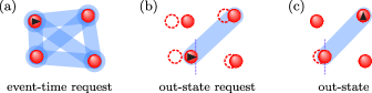
Figure 9: Set of pseudo-factors realized by the end-of-chain event handler. (a): Set of end-of-chain pair pseudo-factors for four point masses coupling the final active unit of the old chain and the beginning active unit of the new chain. (b): At the event time, the realized pseudo-factor with the incoming active unit and the outgoing unit is known. (c): A new event chain is started. The outgoing active unit is shown.

End-of chain event handlers are instances of classes that inherit from the abstract EndOfChainEventHandler class. They effectively stop one event chain and reinitialize a new one. This is often required for the entire run to be irreducible (see [9]). The end-of-chain event handler clearly realizes a set of pseudo-factors, rather than a single pseudo-factor (see Fig. 9a). An end-of-chain event handler implements a method to sample a new direction of motion. In addition, it implements a method to determine a new chain length (that gives the time of the next end-of-chain event) and, finally, the identifiers of the next independent active cnodes. For this, the end-of-chain event handler is aware of all the possible cnode identifiers (see Section 4.2).

On an event-time request, the end-of-chain event handler returns the next candidate event time (computed from the new chain length) and the identifier of the next independent active cnode. The out-state request is accompanied by the current and the succeeding independent active units and their associated branches (see Fig. 9b). For the out-state, the event handler determines the next direction of motion (see Fig. 9c).

A start-of-run event handler (an instance of a class that inherits from the abstract StartOfRunEventHandler class) is the sole event handler whose presence is required. The start-of-run event is the first one to be committed to the global state, because its candidate event time is set equal to the initial time of the run (usually zero) and because the activator will initially only activate the start-of-run event handler. The start-of-run event handler serves two purposes. First, it sets the initial lifting state. Second, the activator uses the start-of-run event handler as an entry point. Its tag (the start_of_run tag in the configuration files of Section 5) is then used to determine the events that should be activated and created thereafter.

The end-of-run event handler (an instance of a class that inherits from the abstract EndOfRunEventHandler class) terminates a run by raising an end-of-run exception and thus ends the mediator loop. An end-of-run event handler is usually connected, on instantiation, with its own output handler. In JF-V1.0, its send_event_time method returns the total run-time, which transits from the configuration file. On the send_out_state request, all active units are time-sliced. The end-of-run output handler may further process the global state which it receives via the mediating method of the end-of-run event handler.

3.3 Event handlers for rigid motion of composite point objects, mode switching

The event handlers of JF-V1.0 are generally suited for the rigid motion of composite point objects (root mode), that is, for independent non-leaf-node units (as implemented in Section 5.2.4). This is possible because all event handlers keep the branches of independent units consistent. As the subtree-node units of an independent-unit node move rigidly, the displacement is not irreducible. Mode switching into leaf mode (with single active leaf units) then becomes a necessity in order to have all factors be considered during one run and to assure the irreversibility of the implemented algorithm. In JF-V1.0, the corresponding event handlers are instances of the RootLeafUnitActiveSwitcher class. On instantiation, they are specified to switch either from leaf mode to root mode or vice versa.

These event handlers resemble the end-of-chain event handler, but only one of them is active at any given time. They provide a method to sample the new candidate event time based on the time stamp of the active independent unit at the time of its activation. An out-state request from one of these event handlers is accompanied by the entire tree of the current independent active unit of one mode and met with the tree of the independent active unit on the alternate mode.

4 JF run specifications and tools

The JF application relies on a user interface to select the physical system that is considered, and to fully specify the algorithm used to simulate it. Inside the application, some of these choices are made available to all modules (rather than having to be communicated repeatedly by the mediator). The application also relies on a number of tools that provide key features to many of its parts.

4.1 Configuration files, logging

The user interface for each run of the JF application consists in a configuration file that is an argument of the executable run.py script. It specifies the physical and algorithmic parameters (temperature, system shape and size, dimension, type of point masses and composite point objects, and also factors, factor potentials, lifting schemes, total run time, sampling frequency, etc).

A configuration file is composed of sections that each correspond to a class requiring input parameters. The [Run] section specifies the mediator and the setting. The ensuing sections choose the parameters in the __init__ methods of the mediator and of the setting. Each section contains pairs of properties and values. The property corresponds to the name of the argument in the __init__ method of the given class, and its value provides the argument (see Fig. 12). The content of the configuration file is parsed by the configparser module and passed to the JF factory (located in the base.factory module) in run.py. Standard Python naming conventions are respected in the classes built by the JF factory, which implies the naming conventions in the configuration file (see Section 6.3 for details). Within the configuration file, sections can be written in any order, but their explicit nesting is not allowed. The nestedness is however implicit in the structure of the configuration file.

The JF application returns all output via files under the control of output handlers. Run-time information is logged (the Python logging module is used). Logged information can range from identification of CPUs to the initialization information of classes, run-time information, etc. Logging output (to standard output or to a file) can take place on a variety of levels from DEBUG to INFO to WARNING that are controlled through arguments of run.py. An identification hash of the run is part of the logging output. It also tags all the output files so that input, output and log files are uniquely linked (the Python uuid module is used).

4.2 Globally used modules

JF-V1.0 requires that all trees representing composite point objects are identical and of height at most two. Furthermore, in the $NVT$ physical ensemble, the particle number, system size and temperature remain unchanged throughout each run. After initialization, as specified in the configuration file, these parameters are stored in the JF  setting package and the modules therein, which may be imported by all other modules, which can then autonomously construct identifiers. Helper functions for periodic boundary conditions (if available) and for the sampling of random positions are also accessible.

JF-V1.0 implements hypercubic and hypercuboid setting modules. Both settings define the inverse temperature and also the attributes of all possible particle identifiers, which are broadcast directly by the setting package. In contrast, the parameters of the physical system are accessed only using the modules of the specific setting (for example the setting.hypercubic_setting module). The setting package and its modules are initialized by classes which inherit from the abstract Setting class. The HypercuboidSetting class defines only the hypercuboid setting, the HypercubicSetting class, however, sets up both the hypercubic_setting and the hypercuboid_setting modules together with the setting package. This allows modules that are specifically implemented for a hypercuboid setting to be used with the hypercubic setting.

Each setting can implement periodic boundaries, by inheriting from the abstract PeriodicBoundaries class and by implementing its methods. Since many modules of JF only rely on periodic boundaries but not on the specific setting, the setting package gives also access to the initialized periodic boundary conditions. Similarly, a function to create a random position is broadcast by the setting package. All the configuration files in Section 5 are for a three-dimensional cubic simulation box, that is, use the hypercubic setting with dimension = 3.

Additional useful modules are located in the JF base package. The abstract Initializer class located in the initializer module enforces the implementation of an initialize method. This method must be called before other public methods of the inheriting class. The strings module provides functions to translate strings from snake to camel case and vice versa, as well as to translate a package path into a directory path. Helper functions for vectors, such as calculating the norm or the dot product, are located in the vectors module.

4.3 Cell systems and cell-occupancy systems

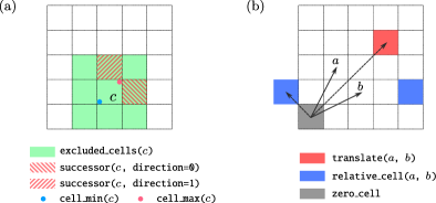
Figure 10: Cell methods. (a): excluded_cells, successor, cell_min and cell_max methods required by the abstract Cells class. Horizontal and vertical directions are indexed as $0$ and $1$, respectively. (b): translate and relative_cell methods (illustrated by vectors) required by the PeriodicCells class, in addition to the methods of the Cells class. Periodic boundary conditions are required, and the two blue cells are identical. The periodic-cell system’s origin is given by the zero_cell property.

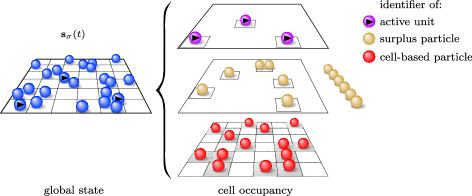
Figure 11: Cell-occupancy system, an internal state of the activator, with active units accounted for differently from surplus and cell-based particles. Only a fixed number of cell-based particle identifiers are allowed per cell (here one per cell). Surplus-particle identifiers may be iterated over from the outside of the cell-occupancy system with a yield_surplus method. In JF-V1.0, surplus particles form an internal dictionary mapping the cell onto the particle identifier.

A cell-occupancy system is an instance of a class that inherits from the abstract CellOccupancy class, located in the activator. Any cell-occupancy system is associated with a cell system, itself an instance of a class that inherits from the abstract Cells class.

In JF-V1.0, the cell system consists in a regular grid of cells that are referred to through their indices. Cells can be iterated over with the yield_cells method. For a given cell, the excluded cells are accessed by the excluded_cells method, the successor cell in a suitably defined direction by the successor method and the lower and upper bound position in each direction through the cell_min and cell_max methods (see Fig. 10a). Finally, the position_to_cell method returns the cell for a given position. Cell systems with periodic boundary conditions are described as periodic cell systems (instances of classes that inherit from the abstract PeriodicCells class, which itself inherits from the Cells class). Their zero_cell property corresponds to the cell located at the origin. Their relative_cell method receives a cell and a reference cell, and establishes equivalence between the relative and the zero-cell. The inverse to this is the translate method (see Fig. 10b).

A cell-occupancy system (which is located in the activator) associates the identifiers of cell-based particles and of surplus particles with a cell. It also stores active cells, that is, cells that contain an active unit (see Fig. 11). Cell-based and surplus particles in the state handler correspond to units with zero velocity, so that there is no real distinction between units and particles for them. The cell-occupancy system inherits from the abstract InternalState class and therefore provides __getitem__ and update methods. The former returns a particle identifier based on a cell, whereas the latter updates the cell occupancies based on the currently active units. This keeps the internal state consistent with the global state. Moreover the cell-occupancy may iterate over surplus particle identifiers via the yield_surplus method. The active cells and the corresponding identifiers of the active units are generated using the yield_active_cells method (see Fig. 11).

JF-V1.0 implements the SingleActiveCellOccupancy class which features only a single active cell and which keeps the active unit identifier among its private attributes. The cell-based particle identifiers are stored in an internal _occupant list, and surplus-particle identifiers are stored in an internal _surplus dictionary mapping the cell indices onto the surplus-particle identifiers.

The stored cell-occupancy system can address different levels of composite particles: one cell-occupancy system may track particles (and units) associated to root nodes, and another one particles that go with leaf nodes. This is set on initialization via the cell_level property which equals the length of the particle identifier tuple. The concerned cell system is itself set on initialization. An indicator charge allows one to select specific particles on a given level for tracking.

A single run can feature several internal states stored within the activator. These instances may rely on different cell-occupancy systems and cell systems. For consistency between internal states and the global state, each cell-occupancy system requires its own cell-boundary event handler.

4.4 Inter-particle potentials and bounding potentials

In JF, potentials play a dual role, as factor potentials $U_{M}$ to event handlers but also as bounding potentials for factor potentials $U_{M}$. Potentials are located in the JF potential package. They inherit from the abstract Potential class and provide a derivative method. They may in addition inherit from the abstract InvertiblePotential class, and must then provide a displacement method. In JF-V1.0, derivatives and displacements are with respect to the positive change of the active unit along one of the coordinates (indicated through the direction). For a potential $U(\mathbf{r}_{ij})$ and direction $=0$, the derivative is for example given by $\left[\partial/\partial x_{i}U(\mathbf{r}_{ij})\right]$.

4.4.1 Inverse-power-law potential, Lennard-Jones potential

The inverse-power-law potential (an instance of the InversePowerPotential class that inherits from the abstract InvertiblePotential class) concerns the separation vector $\mathbf{r}_{ij}=\mathbf{r}_{j}-\mathbf{r}_{i}$ (without periodic boundary conditions, in $d$-dimensional space) between a unit $j$ and an active unit $i$ as

$$U_{(\{i,j\},\,\text{inv})}(\mathbf{r}_{ij},c_{i},c_{j})=c_{i}c_{j}k\left(\frac{1}{|\mathbf{r}_{ij}|}\right)^{p}.$$ (6)

Here, $k$ and $p>0$ correspond to the prefactor and power parameters set on initialization. The charges $c_{i}$ and $c_{j}$ are entered into the methods of the potential as parameters charge_one and charge_two. This allows one instance of the InversePowerPotential class to be used for different charges. The derivative method is straightforward, while the displacement method distinguishes the repulsive ($c_{i}c_{j}k>0$) and the attractive ($c_{i}c_{j}k<0$) cases.

The Lennard-Jones potential (an instance of the LennardJonesPotential class) implements the Lennard-Jones potential

$$U_{\left(\{i,j\},\,\text{\text{LJ}}\right)}(\mathbf{r}_{ij})=k_{\text{LJ}}\left[\left(\frac{\sigma}{|\mathbf{r}_{ij}|}\right)^{12}-\left(\frac{\sigma}{|\mathbf{r}_{ij}|}\right)^{6}\right],$$ (7)

where $\mathbf{r}_{ij}=\mathbf{r}_{j}-\mathbf{r}_{i}$ is the separation vector (without periodic boundary conditions, in $d$-dimensional space) between a unit $j$ and an active unit $i$. and where $k_{\text{LJ}}$ and $\sigma$ correspond to the parameters prefactor and characteristic_length set on instantiation. This Lennard-Jones potential provides a straightforward derivative method. Its displacement method relies on an algebraic inversion.

4.4.2 Displaced-even-power-law potential

An instance of the DisplacedEvenPowerPotential class that inherits from the abstract InvertiblePotential class, the displaced-even-power-law potential, concerns the separation vector $\mathbf{r}_{ij}=\mathbf{r}_{j}-\mathbf{r}_{i}$ (without periodic boundary conditions, in $d$-dimensional space) between a unit $j$ and an active unit $i$

$$U_{(\{i,j\},\,\text{depp})}(\mathbf{r}_{ij})=k_{\text{depp}}\left(|\mathbf{r}_{ij}|-r_{0}\right)^{p},$$ (8)

where $k_{\text{depp}}>0$, $p\in\{2,4,6,\dots\}$, and $r_{0}$, respectively, are the parameters prefactor, power, and equilibrium_separation parameters set on instantiation. The derivative and displacement methods are provided analytically.

4.4.3 Merged-image Coulomb potential and bounding potential

An instance of the MergedImageCoulombPotential class that inherits from the abstract Potential class, the merged-image Coulomb potential is defined for a separation vector $\mathbf{r}_{ij}=\mathbf{r}_{j}-\mathbf{r}_{i}$ (with periodic boundary conditions, in three-dimensional space) between a unit $j$ and an active unit $i$ as

$$U_{\rm C}(\mathbf{r}_{ij},c_{i},c_{j})=\sum_{\mathbf{n}}c_{i}c_{j}/|\mathbf{r}_{ij}+\mathbf{n}\mathbf{L}|,\quad\mathbf{n}\in\mathbb{Z}^{3},$$ (9)

where $\mathbf{L}=(L_{x},L_{y},L_{x})$ are the sides of the three-dimensional simulation box with periodic boundary conditions. The conditionally convergent sum in eq. (9) can be consistently defined in terms of “tin-foil” boundary conditions [21]. It then yields an absolutely convergent sum, partly in real space and partly in Fourier space (see [9, Sect. IIIA]),

$$\psi(\mathbf{r}_{ij},c_{i},c_{j})=c_{i}c_{j}\left[\sum_{\mathbf{n}\in\mathbb{Z}^{3}}\frac{{\rm erfc}(\alpha|\mathbf{r}_{ij}+\mathbf{n}L|)}{|\mathbf{r}_{ij}+\mathbf{n}L|}\right.\left.\!\!+\frac{4\pi}{L^{3}}\!\!\!\sum_{\mathbf{q}\neq(0,0,0)}\!\!\!\!\!\!\frac{\mathrm{e}^{-\mathbf{q}^{2}/(4\alpha^{2})}}{\mathbf{q}^{2}}\cos\left(\mathbf{q}\cdot\mathbf{r}_{ij}\right)\right],$$ (10)

with $\alpha$ a tuning parameter and $\mathbf{q}=2\pi\mathbf{m}/L$, $\mathbf{m}\in\mathbb{Z}^{3}$. JF-V1.0 provides this class for a cubic simulation box, with parameters that are optimized to reach machine precision for its derivative method. Summations over $\mathbf{n}$ and $\mathbf{m}$ are taken within spherical cutoffs, namely for all ${|\mathbf{n}|\leq{\leavevmode\lstinline{{\lst@@@set@language\lst@@@set@numbers\lst@@@set@frame\lst@@@set@rulecolor\lst@@@set@language\lst@@@set@frame{\@listingGroup{ltx_lst_identifier}{position\textunderscore cutoff}}}}}}$ and ${|\mathbf{m}|\leq{\leavevmode\lstinline{{\lst@@@set@language\lst@@@set@numbers\lst@@@set@frame\lst@@@set@rulecolor\lst@@@set@language\lst@@@set@frame{\@listingGroup{ltx_lst_identifier}{fourier\textunderscore cutoff}}}}}}$ except that $\mathbf{m}=(0,0,0)$. (The potential in eq. (10) differs from the tin-foil Coulomb potential in a constant self-energy term that does not influence the derivatives.)

The merged-image Coulomb potential is not invertible. When it serves as a factor potential, bounding potentials provide the required displacement method. JF-V1.0 provides a merged-image Coulomb bounding potential as an instance of the InversePowerCoulombBoundingPotential class, with

$$U_{\rm C,\text{Bounding}}=c_{i}c_{j}k_{b}/{|\mathbf{r}_{ij,0}|}.$$ (11)

Here, $\mathbf{r}_{ij,0}$ is the minimum separation vector, that is, the vector between $\mathbf{r}_{i}$ and the closest image of $\mathbf{r}_{j}$ under the periodic boundary conditions. (The merged-image Coulomb bounding potential thus involves no sum over periodic images.) The constant $k_{b}$ is chosen as

$$k_{b}=\max_{\mathbf{r}\in[-L/2,L/2]^{3}}\frac{|\mathbf{r}|^{3}}{x}\frac{\partial\psi(\mathbf{r})}{\partial x},$$ (12)

so that the factor-potential event rate is bounded. A constant $k_{b}\gtrsim 1.5836$ (the parameter prefactor) is appropriate for a cubic simulation box. The merged-image Coulomb bounding potential is closely related to the inverse-power-law potential of eq. (6) with $p=1$, although the restriction to the minimum separation vector makes that the latter cannot be used directly.

4.4.4 Cell-based bounding potential

A cell-based bounding potential is an instance of a class that inherits from the abstract InvertiblePotential class. It bounds the derivative of the factor potential inside certain cell regions by constants. These constants can be computed analytically on demand or even sampled using a separate Monte Carlo algorithm. On initialization, a cell-based bounding potential receives an estimator (see Section 4.6). Also the information about the cell system is transmitted. Then, the cell-based bounding potential iterates over all pairs of cells (making use of periodic boundary conditions) and determines an upper and lower bound derivative for the factor units being in those cells for each possible direction of motion using the estimator. Here, the cell-based bounding potential is not applied to excluded cells, where the cell-bounded event rate diverges, is simply too large, or otherwise inappropriate.

The constant-derivative bound leads to a piecewise linear invertible bounding potential. The call of the displacement method is accompanied by the direction of motion, the charge product, the sampled potential change and the cell separation. In JF-V1.0, any cell-based bounding potential requires a cell-boundary event handler, that detects when the displacement proposed by the displacement method in fact takes place outside the cell for which it is computed.

4.4.5 Three-body bending potential

The SPC/Fw water model of Section 5.3 includes a bending potential (an instance of the BendingPotential class), which describes the fluctuations in the bond angle within each molecule. For the three units $i$, $j$, and $k$ within such a molecule in three-dimensional space (with $j$ being the oxygen), it is given by

$$U_{(\{i,j,k\},\,\text{\text{bending}})}(\mathbf{r}_{ij},\mathbf{r}_{jk})=\frac{1}{2}k_{b}\Big{(}\phi_{\{i,j,k\}}(\mathbf{r}_{ij},\mathbf{r}_{jk})-\phi_{0}\Big{)}^{2}.$$ (13)

Here, $\phi_{\{i,j,k\}}(\mathbf{r}_{ij},\mathbf{r}_{jk})$ denotes the internal angle between the two hydrogen–oxygen legs. The constants $k_{b}$ and $\phi_{0}$ are set on initialization of the potential (see [9]). The derivative method is provided explicitly for this potential, which is however not invertible.

In JF-V1.0, the associated bounding potential is constructed dynamically by an event handler which dynamically constructs a piecewise linear bounding potential. Here, the event handler speculates on a constant bounding event rate through its position between two subsequent time-sliced positions of the active unit: $q_{\rm bounding}=\max\{q(\mathbf{r}),q(\mathbf{r}+\mathbf{v}\Delta t)\}+\text{const}$ where $q(\mathbf{r})$ is the potential derivative at $\mathbf{r}$. The interval length $|\mathbf{v}\Delta t|$ and the constant offset are input from the configuration file. Fine-tuning provides an efficient bounding potential that does not under-estimate the event rate, yet limits the ratio of unconfirmed events.

4.5 Lifting schemes

Event handlers with more than two independent units require a lifting scheme (an instance of a class that inherits from the Lifting class). The event handler calls a method of the lifting scheme to compute its out-state. At first, the event handler prepares factor derivatives of relevant time-sliced units. The derivative table (see [9, Figs 2 and 10]) is filled with unit identifiers, factor derivatives and activity information through its insert method. Finally, the event handler calls the get_active_identifier method that returns the identifier of the next independent active unit. The lifting scheme’s reset method deletes the derivative table. It is called before the first derivative is inserted. JF-V1.0 implements the ratio, inside-first and outside-first lifting schemes for a single independent active unit (see [9, Sect. IV]).

4.6 Estimator

Estimators (instances of a class that inherits from the abstract Estimator class) determine upper and lower bounds on the factor derivative in a single direction between a minimum and maximum corner of a hypercuboid for the possible separations. For this, they provide the derivative_bound method. Both upper and lower bounds are useful when the potential can have either positive and negative charge products (as happens for example for the merged-image Coulomb potential as a function of the two charges). In general, an estimator compares the factor derivatives for different separations in the hypercuboid to obtain the bounds. These are corrected by a prefactor and optionally by an empirical bound, which are set on instantiation (together with the factor potential).

JF-V1.0 provides estimators which either regard regularly or randomly sampled separations within the hypercuboid. The inner-point and boundary-point estimators vary the separation evenly within the hypercuboid or on the edge of the hypercuboid, respectively. For these separations, the factor potential derivatives (optionally including charges) are compared. Two more estimators consider the interaction between a charged active unit and two oppositely charged target units within a dipole. Here, the factor derivative is summed for the two possible active-target pairs. A Monte-Carlo estimator distributes both the separation and the dipole orientation randomly. The dipole-inner-point estimator varies the separations evenly but aligns the dipole orientation along the direction of the gradient of the factor derivative. The implemented estimators are appropriate for the cookbook examples of Section 5, where the upper and lower bounds on the factor derivatives (and equivalently on the event rates) must be computed for a small number of cell pairs only.

5 JF Cookbook

The configuration files in JF-V1.0 introduce to the key features of the application by constructing runs for two charged point masses, for two interacting dipoles of charges, and for two interacting water molecules (using the SPC/Fw model). All configuration files are for a three-dimensional cubic simulation box with periodic boundary conditions, and they reproduce published data [9].

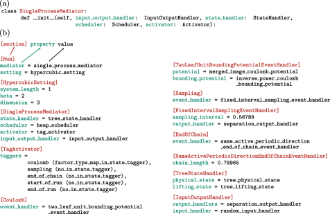
Figure 12: Configuration file coulomb_atoms/power_bounded.ini. (a): A typical __init__ method of a JF class. (b): Excerpts of the configuration file (some lines split for clarity). Sections with properties and values that correspond to the argument names in the __init__ methods of JF classes.

As specified in their [Run] sections, the configuration files use a single-process mediator (an instance of the SingleProcessMediator class), and the setting package is initialized by an instance of the HypercubicSetting class (see for example Fig. 12). All configuration files in the directory use a heap scheduler (an instance of the HeapScheduler class), a tree state handler (instance of the TreeStateHandler class), as well as an tag activator (an instance of the TagActivator class) in order to activate event handlers, trash candidate events and prepare in-states.

The start_of_run, end_of_run, end_of_chain, and sampling event handlers (that realize common pseudo-factors) are implemented in largely analogous sections across all the configuration files, although their parent sections (that define the corresponding taggers) provide different tag lists for trashing and activation of event handlers. The corresponding tagger sections are presented in detail in Section 5.1.1, and only briefly summarized thereafter.

5.1 Interacting atoms

The configuration files in the coulomb_atoms directory of JF-V1.0 implement the ECMC sampling of the Boltzmann distribution for two identical charged point masses. They interact with the merged-image Coulomb pair potential and are described by a Coulomb pair factor. One of the two point masses is active, and it moves either in $+x$, in $+y$, or in $+z$ direction. Statistically equivalent output is obtained for the merged-image Coulomb pair potential (the factor potential) associated with the inverse-power bounding potential (Section 5.1.1), or else with a cell-based bounding potential, either realized directly (Section 5.1.2), or through a cell-veto event handler (Section 5.1.3). Although the configuration files use the language of Section 1.2 for the representation of particles, all trees and branches are trivial, and each root node is also a leaf node.

5.1.1 Atomic factors, inverse-power Coulomb bounding potential

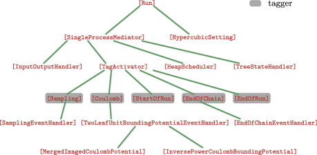
Figure 13: Tree representation the sections in the configuration file coulomb_atoms/power_bounded.ini. Only part of the tree is shown and names of event handlers for sampling and end-of-chain are shortened. The children of the [TagActivator] section correspond to all the declared taggers, which point towards sections for their associated event-handler classes.

The configuration file coulomb_atoms/power_bounded.ini implements a single Coulomb pair factor with the merged-image Coulomb factor potential that is associated with its inverse-power Coulomb bounding potential. The same event handler realizes this factor for any separation of the point masses. The activator requires no internal state.

Although it would be feasible to directly implement (that is, hard-wire) all event handlers for this simple system, the tag activator is used. All event handlers are thus accessed via taggers that are listed, together with their tags, in the [TagActivator] section (see Fig. 13 for a tree representation of the sections). The coulomb tagger is an instance of the FactorTypeMapInStateTagger class, indicating that its event handlers require a specific in-state created from a pattern stored in a file indicated in the [FactorTypeMaps] section. This pattern mirrors the factor index sets and factor types for a system with two root nodes (see eq. (2)). The entry [0, 1], Coulomb in this file indicates that, for two point masses, a Coulomb potential would act between particles 0 and 1. From this information, the tagger’s yield_identifiers_send_event_time method generates all the in-state identifier for any number of point masses.

The [Coulomb] section specifies input for the coulomb tagger’s tag lists (the creates list and the trashes list). Here, a coulomb event creates and trashes only coulomb candidate events (see the configuration file of Section 5.3.1 for different tag lists for the same coulomb event handlers).

The [Coulomb] section further specifies that the coulomb event handler is an instance of the TwoLeafUnitBoundingPotentialEventHandler class and that, for two point masses, only one coulomb event handler is needed. The corresponding section specifies the factor potential to be an instance of the MergedImageCoulombPotential class. It specifies the bounding potential as an instance of the InversePowerCoulombBoundingPotential class. The sampling, end_of_chain, start_of_run and end_of_run taggers are all instances of the NoInStateTagger class (their event handlers require no in-state), and also provide their event handlers and their tag lists, which are then transmitted to the tag activator. Each of these taggers’ yield_identifiers_send_event_time methods yields the in-state identifiers needed by the taggers’ event handlers in order to realize corresponding factors or pseudo-factors.

The configuration file’s [InputOutputHandler] section specifies the input-output handler. It consists of the separation-output handler (an instance of the SeparationOutputHandler class), which is connected to the sampling event handler. In the present example, it samples the nearest-image separation (under periodic boundary conditions) of any two point masses. The initial global physical state is created randomly by the random-input handler (an instance of the RandomInputHandler class). The configuration file coulomb_atoms/power_bounded.ini reproduces published data (see Fig. 14,\raisebox{-.9pt} {2}⃝).

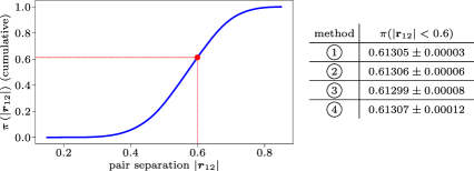
Figure 14: Cumulative histogram of the pair separation $|\mathbf{r}_{12}|$ (nearest image) for two charges in a periodic three-dimensional cubic simulation box with periodic boundary conditions ($\beta c_{1}c_{2}=2$, $L=1$). \raisebox{-.9pt} {1}⃝: Reversible Markov-chain Monte Carlo (see [9, Fig. 8]) \raisebox{-.9pt} {2}⃝: Method of Section 5.1.1 \raisebox{-.9pt} {3}⃝: Method of Section 5.1.2 \raisebox{-.9pt} {4}⃝: Method of Section 5.1.3 , each with standard errors for $\pi(|\mathbf{r}_{12}|<0.6)$.

The configuration file coulomb_atoms/power_bounded.ini can be modified for $N$ point masses. In the [RandomInputHandler] section, the number of root nodes must then equal $N$. In the [Coulomb] section, the number of event handlers must be set to at least $N-1$ (this instructs the Coulomb tagger to deep-copy the required number of event handlers). Without changing the factor-type map with respect to the $N=2$ case, each event handler which will be presented with the correct in-state corresponding to a pair of units with one of them being the active unit. The complexity of the implemented algorithm is $\mathcal{O}(N)$ per event.

5.1.2 Atomic factors, cell-based bounding potential

The configuration file coulomb_atoms/cell_bounded.ini implements a single Coulomb pair factor with the merged-image Coulomb potential, just as the configuration file of Section 5.1.1. However, a cell-occupancy internal state associates the factor potential with a cell-based bounding potential. The target (non-active) unit may be cell-based or surplus (see Fig. 11). The target unit may also be in an excluded nearby cell of the active cell (see Fig. 10), for which the cell-based bounding potential cannot be used. In consequence, three taggers correspond to distinct event handlers that together realize the Coulomb pair factor. The consistency requirement of JF-V1.0 assures that particles and units are always associated with the same cell.

Taggers and their tags are listed in the [TagActivator] section. The coulomb_cell_bounding tagger, for example, appears as an instance of the CellBoundingPotentialTagger class. The coulomb_cell_bounding event handler then realizes the Coulomb factor unless the cell of the target particle is excluded with respect to the active cell and unless it is a surplus particle (in these cases the tagger does not generate any in-state for its event handler). Otherwise, the Coulomb pair factor is realized by a coulomb_surplus-tagged event handler or by a coulomb_nearby event handler. (For two units, as the active unit is taken out of the cell-occupancy system, no surplus candidate events are ever created.)

The cell-occupancy systems (an instance of the SingleActiveCellOccupancy class) is also declared in the [TagActivator] section and further specified in the [SingleActiveCellOccupancy] section. The associated cell system is described in the [CuboidPeriodicCells] section. The internal state, set in the [SingleActiveCellOccupancy] section, has no charge value. This indicates that the identifiers of all particles at the cell level (here cell_level $=1$) are tracked (see Section 5.3.2 for an example where this is handled differently).

The coulomb_nearby tagger, an instance of the ExcludedCellsTagger class, yields the identifiers of particles in excluded cells of the active cell, by iterating over cells and by checking whether they contain appropriate identifiers. The coulomb_surplus tagger similarly relies on the yield_surplus method of the cell-occupancy system to generate in-states.

To keep the internal state consistent with the global state, a cell-boundary event handler is used in the CellBoundaryTagger class (together, this builds cell_boundary candidate events). The cell-boundary tagger just yields the active-unit identifier as the in-state used in the corresponding event handler. The configuration file coulomb_atoms/cell_bounded.ini reproduces published data (see Fig. 14,\raisebox{-.9pt} {3}⃝).

To adapt the configuration file for $N>2$ point masses (from the $N=2$ case that is provided), in the [RandomInputHandler], number_of_root_nodes must be set to $N$. The number of coulomb_cell_bounding, coulomb_nearby, and coulomb_surplus event handlers must be increased. Surplus particles can now exist. The number of event handlers to allow for depends on the cell system, whose parameters must be adapted in order to limit the number of surplus particles, and also to retain useful cell-based bounds for the Coulomb event rates.

5.1.3 Atomic factors, cell-veto

The configuration file coulomb_atoms/cell_veto.ini implements a Coulomb pair factor together with the merged-image Coulomb potential. A cell-occupancy internal state is used. The Coulomb pair factor is then realized, among others, by a cell-veto event handler, which associates the merged-image Coulomb potential with a cell-based bounding potential.

All the Coulomb pair factors of the active particle with target particles that are neither excluded nor surplus are taken together in a set of Coulomb factors, and realized by a single coulomb_cell_veto event handler. The candidate event-time can be calculated with the branch of the active unit as the in-state, which is implemented in the CellVetoTagger class. (The cell-veto tagger returns the identifier of the active unit.) The event handler returns the target cell (in which the candidate unit is to be localized) together with the candidate event time. The out-state request is accompanied by the branch of the target unit (if it exists), and the out-state computation is in analogy with the case studied in Section 5.1.2.

The configuration file features the coulomb_cell_veto tag together with the coulomb_nearby, coulomb_surplus, cell_boundary, sampling, end_of_chain, start_of_run, and end_of_run tags. The configuration file reproduces published data (see Fig. 14,\raisebox{-.9pt} {4}⃝).

To adapt the configuration file for $N$ point masses, the number of root nodes must be set to $N$ in the [RandomInputHandler] section. The number of event handlers for the coulomb_nearby and coulomb_surplus events might have to be increased. However, a single cell-veto event handler realizes any number of factors with cell-based target particles whereas in Section 5.1.2 each of them required its own event handler.

5.2 Interacting dipoles

The configuration files in the dipoles directory of JF-V1.0 implement the ECMC sampling of the Boltzmann distribution for two identical finite-size dipoles, for a model that was introduced previously [9]. Point masses in different dipoles interact via the merged-image Coulomb potential (pairs $1-3$, $1-4$, $2-3$, $2-4$ in Fig. 15). Point masses within each dipole interact with a short-ranged potential (pairs $1-2$ and $3-4$). A repulsive short-range potential between oppositely charged atoms in different dipoles counterbalances the attractive Coulomb potential at small distances (pairs $1-4$ and $2-3$).

Each dipole is a composite point object made up of two oppositely charged point masses. It is represented as a tree with one root node that has two children. The number of root nodes in the system is set in the [RandomInputHandler] section of the configuration file, where the dipoles are created randomly through the fill_root_node method in the DipoleRandomNodeCreator class. In the setting package, the input handler specifies that there are two root nodes (number_of_root_nodes $=2$). Each of them contains two nodes (which is coded as number_of_nodes_per_root_node $=2$) and the number of node levels is two (number_of_node_levels $=2$). As this numbers are set in the setting package, all the JF modules can autonomously construct all possible particle identifiers.

Statistically equivalent output is obtained for pair factors for all interactions (Section 5.2.1), for dipole–dipole Coulomb factors and their factor potential associated with a cell-based bounding potential (Section 5.2.2), for dipole–dipole Coulomb factors with the cell-veto algorithm (Section 5.2.3), and by alternating between concurrent moves of the entire dipoles with moves of the individual point masses (Section 5.2.4). The latter example showcases the collective-motion possibilities of ECMC integrated into JF. All configuration files here implement the short-ranged potential as an instance of the DisplacedEvenPowerPotential class with power $=2$ and the repulsive short-range potential as an instance of the InversePowerPotential class with power $=6$.

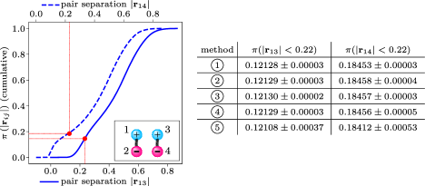
Figure 15: Cumulative histogram of the pair separation $|\mathbf{r}_{13}|$ and $|\mathbf{r}_{14}|$ (nearest image) for two dipoles (see the inset) in a periodic three-dimensional cubic simulation box with periodic boundary conditions ($\beta c_{i}c_{j}=\pm 1$, $L=1$). \raisebox{-.9pt} {1}⃝: Reversible Markov-chain Monte Carlo (see [9, Fig. 11]) \raisebox{-.9pt} {2}⃝: Method of Section 5.2.1 \raisebox{-.9pt} {3}⃝: Method of Section 5.2.2 \raisebox{-.9pt} {4}⃝: Method of Section 5.2.3 \raisebox{-.9pt} {5}⃝: Method of Section 5.2.4, each with standard errors for $\pi(|\mathbf{r}_{13}|<0.22)$ and $\pi(|\mathbf{r}_{14}|<0.22)$.

5.2.1 Atomic Coulomb factors

The configuration file dipoles/atom_factors.ini implements for each concerned pair of point masses a Coulomb pair factor, with the merged-image Coulomb potential associated with the the inverse-power Coulomb bounding potential. Several event handlers that are instances of the same class realize these factors, and the number of event handlers must scale with their number. No internal state is declared. Pair factors are implemented for each pair of point masses that interact with a harmonic or a repulsive potential. One of the four point masses is active at each time, and it moves either in $+x$, in $+y$, or in $+z$ direction. The configuration file represents composite point objects as trees with two levels (see Section 1.2). Positions and velocities are kept consistent on both levels, although the root-unit properties are not made use of. The tree structure only serves to identify leaf units on the same dipole.

In the configuration file, taggers and tags are listed in the [TagActivator] section. The coulomb, harmonic, and repulsive taggers are separate instances of the same FactorTypeMapInStateTagger class, and the corresponding sections set up the corresponding event handlers. Both the harmonic and the repulsive event handlers are instances of the TwoLeafUnitEventHandler class. Aliasing nevertheless assures a tree-structured configuration file (the harmonic tagger is for example declared with a HarmonicEventHandler class which is an alias for the TwoLeafUnitEventHandler class). The coulomb tagger and its event handlers are treated as in Section 5.1.1.

The sampling, start-of-run, end-of-run and end-of-chain pseudo-factors are realized by event handlers that are set up in the same way as in all other configuration files. However, the parent sections differ: the parent of the [InitialChainStartOfRunEventHandler] section sets the start_of_run tagger, which specifies that after the start_of_run event, new coulomb, harmonic, repulsive, sampling end_of_chain, and end_of_run event handlers must be activated. The tag lists thus differ from those of the [StartOfRun] section in other configuration files. The configuration file dipoles/atom_factors.ini reproduces published data (see Fig. 15,\raisebox{-.9pt} {2}⃝).

5.2.2 Molecular Coulomb factors, cell-based bounding potential

The configuration file dipoles/cell_bounded.ini implements for each pair of dipoles a Coulomb four-body factor. (The sum of the merged-image Coulomb potentials for pairs $1-3$, $1-4$, $2-3$, $2-4$ in Fig. 15 constitutes the Coulomb factor potential.) The event rates for such factors decay much faster with distance than for Coulomb pair factors, and the chosen lifting scheme considerably influences the dynamics (see [9, Sect. IV]). The configuration file installs a cell-occupancy internal state on the dipole level (rather than for the point masses). A cell-bounded event handler then realizes a Coulomb four-body factor with its factor potential associated with an orientation-independent cell-based bounding potential for dipole pairs that are not in excluded cells relative to each other. The configuration file furthermore implements pair factors for the harmonic and the repulsive interactions. One of the four point masses is active at each time, and it moves either in $+x$, in $+y$, or in $+z$ direction.

The configuration file’s [TagActivator] section defines all taggers and their corresponding tags. Among the taggers for event handlers realizing the Coulomb four-body factor, the coulomb_cell_bounding tagger differs markedly from the set-up in Section 5.1.2, as the event handler is for a pair of composite point objects. The lifting scheme is set to inside_first_lifting. The bounding potential is defined in the [CellBoundingPotential] section. A dipole Monte Carlo estimator is used for simplicity (see Section 4.6). As it obtains an upper bound for the event rate from random trials for each relative cell orientations, its use is restricted to there being only a small number of cells. The coulomb_nearby and coulomb_surplus taggers are for event handlers realizing the Coulomb four-body factor when the bounding potential cannot be used. In this case, the merged-image Coulomb potential is summed for the factor potential, but also for the bounding potential. The standard sampling, end_of_chain, end_of_run, start_of_run taggers as well as the ones responsible for the harmonic and repulsive potentials are set up in a similar way as in Section 5.2.1.

The [TagActivator] section defines the internal state that is used by the coulomb_cell_bounding, coulomb_nearby, and coulomb_surplus taggers. The [SingleActiveCellOccupancy] section specifies the cell level (cell_level $=1$ indicates that the particle identifiers have length one, corresponding to root nodes, rather than length two, which would correspond to the dipoles’ leaf nodes). Positions and velocities must thus be kept consistent on both levels. The cell-occupancy system requires the presence of a cell_boundary event handler, again on the level of the root nodes. This event handler is aware of the cell level, and it ensures consistency of the events triggered by the cell-based bounding potential with the underlying cell system. The configuration file dipoles/cell_bounded.ini reproduces published data (see Fig. 15,\raisebox{-.9pt} {3}⃝).

5.2.3 Molecular Coulomb factors, cell-veto

The configuration file dipoles/cell_veto.ini implements the same factors and pseudo-factors and the same internal state as the configuration file of Section 5.2.2. A single cell-veto event handler then realizes the set of factors that relate to cells that are not excluded for any number of cell-based particles, whereas in the earlier implementation, the number of cell-bounded event handlers must exceed the possible number of particles in non-excluded cells of the active cell. This is what allows to implement ECMC with a complexity of $\mathcal{O}(1)$ per event.

The configuration file resembles that of Section 5.2.2. It mainly replaces the latter file’s coulomb_cell_bounding event handlers with a coulomb_cell_veto event handler. Slight differences reflect the fact that a cell-veto event handler uses no displacement method of the bounding potential but obtains the displacement from the total event rate (see the discussion in Section 3.1.3). The configuration file dipoles/cell_veto.ini reproduces published data (see Fig. 15,\raisebox{-.9pt} {4}⃝).

5.2.4 Atomic Coulomb factors, alternating root mode and leaf mode

The configuration file dipoles/dipole_motion.ini implements two different modes. In leaf mode, at each time one of the four point masses is active, and it moves either in $+x$, in $+y$, or in $+z$ direction (see Fig. 16a). In root mode, at each time the point masses of one dipole moves as a rigid block, in the same direction (see Fig. 16b). (The root mode, by itself, does not assure irreducibility of the Markov-chain algorithm, as the orientation and shape of any dipole molecule would remain unchanged throughout the run.)

JF-V1.0 represents the dipoles as trees, and both modes are easily implemented. In leaf mode, the Coulomb factors are realized by coulomb_leaf event handlers that are instances of the same class as the coulomb_nearby event handlers in Sections 5.2.2 and 5.2.3. The root mode, in turn, is patterned after the simulation of two point masses (as in Section 5.1.1): all inner-dipole potentials are constant. The inter-dipole Coulomb potentials sum up to an effective two-body potential, the factor potential of a two-body factor realized in a Coulomb-dipole event handler. The repulsive short-range potential between oppositely charged atoms in different dipoles also translates into a potential between the dipoles in rigid motion, and serves as a factor potential of a two-body factor, realized in a specific event handler.

Taggers and their tags are listed in the [TagActivator] section. The harmonic_leaf, repulsive_leaf (leaf-mode) taggers, as well as all those related to event handlers that realize pseudo-factors are as in Section 5.2.1. The coulomb_leaf tagger corresponds to the coulomb_nearby tagger in Section 5.2.2. The coulomb_root and repulsive_root taggers are analogous to those in Section 5.1.1 for the two-atom case.

As all other operations that take place in JF, the switches between leaf mode and root mode are also formulated as events. They are related to two pseudo-factors and realized by a leaf_to_root event handler and by a root_to_leaf event handler, respectively. (These two event handlers are aliases for instances of the RootLeafUnitActiveSwitcher class.) The root_to_leaf and leaf_to_root taggers, in addition to the create and trash lists, set up separate activate and deactivate lists (see Section 2.4). The configuration file reproduces published data (see Fig. 15,\raisebox{-.9pt} {5}⃝). Of particular interest is that the tree representation of composite point objects keeps consistency between leaf-node units and root-node units: the event handlers return branches of cnodes for all independent units (see Fig. 7) whose unit information can be integrated into the global state.

Figure 16: Two moves implemented in dipoles/dipole_motion.ini. (a): In leaf mode, a single independent active leaf unit has velocity $\mathbf{v}$. The corresponding dipole center (the active root unit) is induced to move at $\mathbf{v}/2$. (b): In root mode, one dipole (independent active root unit) has velocity $\mathbf{v}$, and both its active leaf units have induced velocity $\mathbf{v}$.

5.3 Interacting water molecules (SPC/Fw model)

The configuration files in the water directory implement the ECMC sampling of the Boltzmann distribution for two water molecules, using the SPC/Fw model that was previously studied with ECMC [9]. Molecules are represented as composite point objects with three charged point masses, one of which is positively charged (representing the oxygen) and the two others are negatively charged (representing the hydrogens). Point masses in different water molecules interact via the merged-image Coulomb potential. In addition, point masses within each molecule interact with a three-body bending interaction, and a harmonic oxygen–hydrogen potential. Finally, any two oxygens interact through a Lennard-Jones potential [9].

In the tree state handler (defined in the [TreeStateHandler] section, a child of the [SingleProcessMediator] section), water molecules are represented as trees with a root node and three children (the leaf nodes of the tree). The total number of water molecules (that is, of root nodes) is set in the [RandomInputHandler] section of each configuration file. The molecules are created through the fill_root_node method in the WaterRandomNodeCreator class. There are two node levels (number_of_node_levels $=2$) and three nodes per root node (number_of_nodes_per_root_node $=3$). The charges of a molecule are set in the [ElectricChargeValues] section (a descendant of the [WaterRandomNodeCreator] section).

All the configuration files in the water directory of JF-V1.0 implement the pair harmonic factors that are realized through harmonic event handlers. The corresponding taggers are defined in the [Harmonic] sections, with the displaced even-power potential and its parameters set in the [HarmonicEventHandler] and [HarmonicPotential] sections. The configuration files furthermore implement the taggers corresponding to the three-body bending factors in their [Bending] sections. The bending event handler has three independent units (attached to branches). It thus requires a lifting scheme (which is chosen in the [BendingEventHandler] section), which is however unique (see [9, Fig. 2]). In all these configuration files, one of the six point masses is active, and it moves either in $+x$, in $+y$, or in $+z$ direction (the optional rigid displacement of the entire water molecule, could be set up as in Section 5.2.4).

Statistically equivalent output is obtained for a simple set-up featuring pair factors for the Coulomb potential and a Lennard-Jones interaction that is inverted (Section 5.3.1), or for a molecular-factor Coulomb potential associated with a power-law bounding potential and a cell-based Lennard-Jones bounding potential (Section 5.3.2). In addition, the cell-veto algorithm for the Coulomb potential coupled to an inverted Lennard-Jones potential (Section 5.3.3) is also provided. Finally, cell-veto event handlers take part in the realization of complex molecular Coulomb factors and also realize Lennard-Jones factors between oxygens (Section 5.3.4). This illustrates how multiple independent cell-occupancy systems may coexist within the same run.

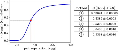
Figure 17: Cumulative histogram of the oxygen–oxygen pair separation $|\mathbf{r}_{\text{OO}}|$ for two SPC/Fw water molecules in a periodic cubic simulation box. \raisebox{-.9pt} {1}⃝: Reversible Markov-chain Monte Carlo (see [9, Fig. 14]) \raisebox{-.9pt} {2}⃝: Method of Section 5.3.1 \raisebox{-.9pt} {3}⃝: Method of Section 5.3.2 \raisebox{-.9pt} {4}⃝: Method of Section 5.3.3 \raisebox{-.9pt} {5}⃝: Method of Section 5.3.4, each with standard errors for $\pi(|\mathbf{r}_{\text{OO}}|<2.9)$.

5.3.1 Atomic Coulomb factors, Lennard-Jones inverted

The configuration file water/coulomb_power_bounded_lj_inverted.ini implements pair Lennard-Jones, harmonic and Coulomb factors. The Coulomb factors are realized for any distance of the point masses by event handlers that associate the merged-image Coulomb potential with its inverse-power Coulomb bounding potential. The Lennard-Jones potential is inverted. This configuration file needs no internal state.

In the configuration file, the [TagActivator] section lists all the taggers together with their tags, which in addition to the taggers related to pseudo-factors, are reduced to coulomb, harmonic, bending, and lennard_jones. The merged-image Coulomb potential with its associated power-law bounding potential (both for attractive and repulsive charge products) is specified in the [Coulomb] section of the configuration file. The Lennard-Jones potential is invertible and its displacement method is used rather than that of a bounding potential. The output handler is defined in the [OxygenOxygenSeparationOutputHandler] section, a child of the [InputOutputHandler] section. It obtains all the units, extracts the oxygens through their unit identifier, and records the oxygen–oxygen separation distance. This reproduces published data (see Fig. 17,\raisebox{-.9pt} {2}⃝).

5.3.2 Molecular Coulomb factors, Lennard-Jones cell-bounded

The configuration file water/coulomb_power_bounded_lj_cell_bounded.ini for the water system corresponds to pair factors for the Lennard-Jones and the harmonic potentials and to molecular factors for the Coulomb interaction. The Coulomb factor potential is the sum of the merged-image Coulomb potential for the nine relevant pairs of point masses (pairs across two molecules). It is realized in a particular event handler, analogously to how this is done for the Coulomb interaction in Sections 5.2.2 and 5.2.3. The associated bounding potential (both for attractive and repulsive charge combinations) is given by the sum over all the individual pairs. Although the Lennard-Jones interaction can be inverted, the configuration file sets up a cell-occupancy internal state that tracks the identifiers for the oxygens. As in previous cases, this leads to three types of events, corresponding to the nearby, surplus, and cell-based particles, in addition to cell-boundary events.

Taggers and their tags are listed in the [TagActivator] section. Taggers are generally utilized as in other configuration files. The internal state is specified in the [TagActivator] section. As set up in the [SingleActiveCellOccupancy] section, it features a oxygen_indicator charge (set in the [OxygenIndicator] section). The oxygen-indicator charge is non-zero only for the oxygens. In consequence, the oxygen cell system (defined in the [OxygenCell] section) tracks only oxygens. This reproduces published data (see Fig. 17,\raisebox{-.9pt} {3}⃝). Nevertheless, this configuration file does not scale up easily with system size.

5.3.3 Molecular Coulomb cell-veto, Lennard-Jones inverted

The configuration file water/coulomb_cell_veto_lj_inverted.ini for the water system corresponds to the same factors as in Section 5.3.2. As a preliminary step towards the treatment of all long-range interactions with the cell-veto algorithm, in Section 5.3.4, molecular Coulomb factors are realized here (for non-excluded cells of the active cell) with a cell-veto event handler.

Taggers and their tags are listed in the [TagActivator] section, and they are generally similar to those of other configuration files. In addition, the internal state for the Coulomb system is defined in the [TagActivator] section and further described in the [SingleActiveCellOccupancy] section. The latter describes the cell level (which serves for the water molecules) as on the root node level (cell_level $=1$), the barycenter of the leaf-node positions of each water molecule. (Root-node and leaf-node positions are set in the random input handler, which itself uses a water random node creator.)

The event handlers consistently update all leaf-node positions and root-node positions from a valid initial configuration obtained in an instance of the WaterRandomNodeCreator class. Consistency will be deteriorated over long runs, but this is of little importance for the simple example case presented here. The configuration file reproduces published data (see Fig. 17,\raisebox{-.9pt} {4}⃝).

5.3.4 Molecular Coulomb cell-veto, Lennard-Jones cell-veto

The configuration file water/coulomb_cell_veto_lj_cell_veto.ini offers no new factors compared to Sections 5.3.2 and 5.3.3, but it uses, for illustration purposes, two cell-occupancy systems and two cell-veto event handlers. As nearby and surplus particles are excluded from the cell-veto treatment, this implies two sets of cell-based, nearby, and surplus event handlers in addition to two cell-boundary event handlers. For the molecular Coulomb factors, the cell-veto event handler receives as a factor potential the sum of pairwise merged-image Coulomb potentials with attractive and repulsive charge combinations. Cells track the barycenter of individual water molecules, and consistency between root-node units and leaf-node units is of importance. Although the Lennard-Jones potential can be inverted, the configuration file sets up a second cell-occupancy system for the Lennard-Jones potential. The cell-occupancy system tracks only leaf-node particles that correspond to oxygen atoms.

Taggers and their tags are listed in the [TagActivator] section. This section is of interest as it sets up the internal state as two cell-occupancy systems, both instances of the same SingleActiveCellOccupancy class. They require different parameters, and are therefore presented under aliases, in the [OxygenCell] and [MoleculeCell] sections. Each of theses cell-occupancy systems use a separate cell system instance of the same class. As the two cell systems have the same parameters, they do not need to be aliased in the configuration file. The configuration file reproduces published data (see Fig. 17,\raisebox{-.9pt} {5}⃝).

6 Licence, GitHub repository, Python version

JF, the Python application described in this paper, is an open-source software project that grants users the rights to study and execute, modify and distribute the code. Modifications can be fed back into the project.

6.1 Licence information, used software

JF is made available under the GNU GPLv3 licence (for details see the JF LICENCE file). The use of the Python MDAnalysis package [27, 11] for reading and writing .pdb files, of the Python Dill package [25, 26] for dumping and restarting a run of the application, and of the Python Matplotlib [15] and NumPy [31, 38] packages for the graphical analysis of output is acknowledged.

6.2 GitHub repository

JeLLyFysh, the public repository for all the code and the documentation of the application, is part of a public GitHub organization. The repository can be forked (that is, copied to an outside user’s own public repository) and from there studied, modified and run in the user’s local environment. Users may contribute to the JF application via pull requests (see the JF README and CONTRIBUTING.md files for instructions and guidelines). All communication (bug reports, suggestions) takes place through GitHub “Issues”, that can be opened in the repository by any user or contributor, and that are classified in GitHub projects on JeLLyFysh.

6.3 Python version, coding conventions

JF-V1.0 is compatible with Python 3.5 (and higher) and with PyPy 7 (and higher), a just-in-time compiling Python alternative to interpreted CPython (see the JF documentation for details). JF code adheres to the PEP8 style guide for Python code, except for the linewidth that is set to 120 (see the CONTRIBUTING.md file for details).

Following the PEP8 Python naming convention, JF modules and packages are spelled in snake case and classes in camel case (the state_handler module thus contains the StateHandler class). In configuration files, section titles are in camel case and enclosed in square brackets (see Fig. 13).

Versioning of the JF project adopts two-to-four-field version numbers defined as Milestone.Feature.AddOn.Patch. Version 1.0, as described, represents the first development milestone which reproduces published data [9]. Patches and bugfixes of this version will be given number 1.0.0.1, 1.0.0.2, etc. (Finer-grained distinction between versions is obtained through the hashes of master-branch GitHub commits.) New configuration files and required extensions are expected to lead to versions 1.0.1. 1.0.2, etc. Version 1.1 is expected to fully implement different dimensions and arbitrary rectangular and cuboid shapes of the JF potential package. Versions 1.2 and 1.3 will consistently implement $n_{\text{ac}}>1$ independent active particles (on a single processor) and eliminate unnecessary time-slicing for some events triggered by pseudo-factors and for unconfirmed events. All development from Versions 1.0 to 2.0 can be undertaken concurrently. Fully parallel code is planned for Version 3.0. In JF development, two-field versions (2.0, 3.0, etc) may introduce incompatible code, while three- and four-field version numbers are intended to be backward compatible.

7 Conclusions, outlook

As presented in this paper, JF is a computer application for ECMC simulations that is hoped to become useful for researchers in different fields of computational science. The JF-V1.0 constitutes its first development milestone: built on the mediator design pattern, it systematically formulates the entire ECMC time evolution in terms of events, from the start-of-run to the end-of-run, including sampling, restarts (that is, end-of-chain), and the factor events. A number of configuration files validate JF-V1.0 against published test cases for long-range interacting systems [9].

For JF-V1.0, consistency has been the main concern, and code has not yet been optimized. Also, the handling of exceptions remains rudimentary, although this is not a problem for the cookbook examples of Section 5.

All the methods are written in Python. Considerable speed-up can certainly be obtained by rewriting time-consuming parts of the application in compiled languages, in particular of the potential package. One of the principal limitations of JF-V1.0 is that pseudo-factor-related and unconfirmed events are time-sliced, leading to superfluous trashing and re-activation of candidate events. Optimized bounding potentials for many-particle factor potentials appear also as a priority.

The consistent implementation of an arbitrary number $n_{\text{ac}}$ of simultaneously active particles is straightforward, although it has also not been implemented fully in JF-V1.0. (As mentioned, this is planned for JF (Version 2.0)). This will enable full parallel implementations on multiprocessor machines. Simplified parallel implementations for one-dimensional systems and for hard-disk models in two dimensions are currently being prototyped. The parallel computation of candidate events (using the MultiProcessMediator class implemented in JF-V1.0) is at present rather slow. Bringing the full power of parallelization and of multi-process ECMC to real-world applications appears as its outstanding challenge for JF.

References

- Alder and Wainwright [1957] Alder, B.J., Wainwright, T.E., 1957. Phase Transition for a Hard Sphere System. J. Chem. Phys. 27, 1208–1209. doi:10.1063/1.1743957.
- Alder and Wainwright [1959] Alder, B.J., Wainwright, T.E., 1959. Studies in Molecular Dynamics. I. General Method. J. Chem. Phys. 31, 459–466. doi:10.1063/1.1730376.
- Bannerman and Lue [2010] Bannerman, M.N., Lue, L., 2010. Exact on-event expressions for discrete potential systems. J. Chem. Phys. 133, 124506–124506. doi:10.1063/1.3486567.
- Bernard and Krauth [2011] Bernard, E.P., Krauth, W., 2011. Two-Step Melting in Two Dimensions: First-Order Liquid-Hexatic Transition. Phys. Rev. Lett. 107, 155704. URL: http://link.aps.org/doi/10.1103/PhysRevLett.107.155704, doi:10.1103/PhysRevLett.107.155704.
- Bernard et al. [2009] Bernard, E.P., Krauth, W., Wilson, D.B., 2009. Event-chain Monte Carlo algorithms for hard-sphere systems. Phys. Rev. E 80, 056704. URL: http://link.aps.org/doi/10.1103/PhysRevE.80.056704, doi:10.1103/PhysRevE.80.056704.
- Bierkens et al. [2017] Bierkens, J., Bouchard-Côté, A., Doucet, A., Duncan, A.B., Fearnhead, P., Roberts, G., Vollmer, S.J., 2017. Piecewise Deterministic Markov Processes for Scalable Monte Carlo on Restricted Domains arXiv:1701.04244.
- Diaconis et al. [2000] Diaconis, P., Holmes, S., Neal, R.M., 2000. Analysis of a nonreversible Markov chain sampler. Annals of Applied Probability 10, 726–752.
- Ding et al. [2008] Ding, F., Tsao, D., Nie, H., Dokholyan, N.V., 2008. Ab Initio Folding of Proteins with All-Atom Discrete Molecular Dynamics. Structure 16, 1010–1018. URL: https://doi.org/10.1016/j.str.2008.03.013, doi:10.1016/j.str.2008.03.013.
- Faulkner et al. [2018] Faulkner, M.F., Qin, L., Maggs, A.C., Krauth, W., 2018. All-atom computations with irreversible Markov chains. The Journal of Chemical Physics 149, 064113. URL: https://doi.org/10.1063/1.5036638, doi:10.1063/1.5036638.
- Gamma et al. [1994] Gamma, E., Helm, R., Johnson, R., Vlissides, J.M., 1994. Design Patterns: Elements of Reusable Object-Oriented Software. 1 ed., Addison-Wesley Professional.
- Gowers et al. [2016] Gowers, R., Linke, M., Barnoud, J., Reddy, T., Melo, M., Seyler, S., Domański, J., Dotson, D., Buchoux, S., Kenney, I., Beckstein, O., 2016. MDAnalysis: A Python Package for the Rapid Analysis of Molecular Dynamics Simulations, in: Proceedings of the 15th Python in Science Conference, SciPy. URL: https://doi.org/10.25080/majora-629e541a-00e, doi:10.25080/majora-629e541a-00e.
- Harland et al. [2017] Harland, J., Michel, M., Kampmann, T.A., Kierfeld, J., 2017. Event-chain Monte Carlo algorithms for three- and many-particle interactions. EPL (Europhysics Letters) 117, 30001. URL: http://stacks.iop.org/0295-5075/117/i=3/a=30001.
- Hasenbusch and Schaefer [2018] Hasenbusch, M., Schaefer, S., 2018. Testing the event-chain algorithm in asymptotically free models. Phys. Rev. D 98, 054502. URL: https://link.aps.org/doi/10.1103/PhysRevD.98.054502, doi:10.1103/PhysRevD.98.054502.
- Herbordt et al. [2009] Herbordt, M.C., Khan, M.A., Dean, T., 2009. Parallel Discrete Event Simulation of Molecular Dynamics Through Event-Based Decomposition, in: 2009 20th IEEE International Conference on Application-specific Systems, Architectures and Processors, IEEE. URL: https://doi.org/10.1109/asap.2009.39, doi:10.1109/asap.2009.39.
- Hunter [2007] Hunter, J.D., 2007. Matplotlib: A 2D Graphics Environment. Computing in Science & Engineering 9, 90–95. URL: https://doi.org/10.1109/mcse.2007.55, doi:10.1109/mcse.2007.55.
- Kapfer and Krauth [2013] Kapfer, S.C., Krauth, W., 2013. Sampling from a polytope and hard-disk Monte Carlo. Journal of Physics: Conference Series 454, 012031. URL: http://stacks.iop.org/1742-6596/454/i=1/a=012031, doi:10.1088/1742-6596/454/1/012031.
- Kapfer and Krauth [2015] Kapfer, S.C., Krauth, W., 2015. Two-Dimensional Melting: From Liquid-Hexatic Coexistence to Continuous Transitions. Phys. Rev. Lett. 114, 035702. URL: http://link.aps.org/doi/10.1103/PhysRevLett.114.035702, doi:10.1103/PhysRevLett.114.035702.
- Kapfer and Krauth [2016] Kapfer, S.C., Krauth, W., 2016. Cell-veto Monte Carlo algorithm for long-range systems. Phys. Rev. E 94, 031302. URL: http://link.aps.org/doi/10.1103/PhysRevE.94.031302, doi:10.1103/PhysRevE.94.031302.
- Kapfer and Krauth [2017] Kapfer, S.C., Krauth, W., 2017. Irreversible Local Markov Chains with Rapid Convergence towards Equilibrium. Phys. Rev. Lett. 119, 240603. URL: https://link.aps.org/doi/10.1103/PhysRevLett.119.240603, doi:10.1103/PhysRevLett.119.240603.
- Khan and Herbordt [2011] Khan, M.A., Herbordt, M.C., 2011. Parallel discrete molecular dynamics simulation with speculation and in-order commitment. Journal of Computational Physics 230, 6563 – 6582. URL: http://www.sciencedirect.com/science/article/pii/S0021999111002968, doi:https://doi.org/10.1016/j.jcp.2011.05.001.
- de Leeuw et al. [1980] de Leeuw, S.W., Perram, J.W., Smith, E.R., 1980. Simulation of electrostatic systems in periodic boundary conditions. II. Equivalence of boundary conditions. Proc. R. Soc. A 373, 57–66. URL: http://rspa.royalsocietypublishing.org/content/373/1752/57, doi:10.1098/rspa.1980.0136.
- Lei and Krauth [2018a] Lei, Z., Krauth, W., 2018a. Irreversible Markov chains in spin models: Topological excitations. EPL 121, 10008.
- Lei and Krauth [2018b] Lei, Z., Krauth, W., 2018b. Mixing and perfect sampling in one-dimensional particle systems. EPL 124, 20003. URL: http://stacks.iop.org/0295-5075/124/i=2/a=20003.
- Lei et al. [2019] Lei, Z., Krauth, W., Maggs, A.C., 2019. Event-chain Monte Carlo with factor fields. Physical Review E 99. URL: https://doi.org/10.1103/physreve.99.043301, doi:10.1103/physreve.99.043301.
- McKerns and Aivazis [2010] McKerns, M.M., Aivazis, M.A., 2010. Pathos: a framework for heterogeneous computing. URL: http://trac.mystic.cacr.caltech.edu/project/pathos.
- McKerns et al. [2011] McKerns, M.M., Strand, L., Sullivan, T., Fang, A., Aivazis, M.A., 2011. Building a Framework for Predictive Science , in: van der Walt, S., Millman, J. (Eds.), Proceedings of the 10th Python in Science Conference, pp. 67 – 78.
- Michaud-Agrawal et al. [2011] Michaud-Agrawal, N., Denning, E.J., Woolf, T.B., Beckstein, O., 2011. MDAnalysis: A toolkit for the analysis of molecular dynamics simulations. Journal of Computational Chemistry 32, 2319–2327. URL: https://doi.org/10.1002/jcc.21787, doi:10.1002/jcc.21787.
- Michel et al. [2014] Michel, M., Kapfer, S.C., Krauth, W., 2014. Generalized event-chain Monte Carlo: Constructing rejection-free global-balance algorithms from infinitesimal steps. J. Chem. Phys. 140, 054116. doi:10.1063/1.4863991, arXiv:1309.7748.
- Miller and Luding [2003] Miller, S., Luding, S., 2003. Event-driven molecular dynamics in parallel. Journal of Computational Physics 193, 306–316. URL: https://doi.org/10.1016/j.jcp.2003.08.009, doi:10.1016/j.jcp.2003.08.009.
- Nishikawa et al. [2015] Nishikawa, Y., Michel, M., Krauth, W., Hukushima, K., 2015. Event-chain algorithm for the Heisenberg model: Evidence for z sim 1 dynamic scaling. Phys. Rev. E 92, 063306. doi:10.1103/PhysRevE.92.063306, arXiv:1508.05661.
- Oliphant [2006] Oliphant, T.E., 2006. A guide to NumPy. Trelgol Publishing USA.
- Peters and de With [2012] Peters, E.A.J.F., de With, G., 2012. Rejection-free Monte Carlo sampling for general potentials. Phys. Rev. E 85, 026703. URL: http://link.aps.org/doi/10.1103/PhysRevE.85.026703, doi:10.1103/PhysRevE.85.026703.
- Proctor et al. [2011] Proctor, E.A., Ding, F., Dokholyan, N.V., 2011. Discrete molecular dynamics. Wiley Interdisciplinary Reviews: Computational Molecular Science 1, 80–92. URL: https://onlinelibrary.wiley.com/doi/abs/10.1002/wcms.4, doi:10.1002/wcms.4, arXiv:https://onlinelibrary.wiley.com/doi/pdf/10.1002/wcms.4.
- Proctor and Dokholyan [2016] Proctor, E.A., Dokholyan, N.V., 2016. Applications of Discrete Molecular Dynamics in biology and medicine. Current Opinion in Structural Biology 37, 9 – 13. URL: http://www.sciencedirect.com/science/article/pii/S0959440X15001578, doi:https://doi.org/10.1016/j.sbi.2015.11.001. theory and simulation - Macromolcular machines.
- Qin et al. [2019] Qin, L., Höllmer, P., Maggs, A.C., Krauth, W., 2019. Benchmarking ECMC against Lammps. Manuscript in preparation.
- Shirvanyants et al. [2012] Shirvanyants, D., Ding, F., Tsao, D., Ramachandran, S., Dokholyan, N.V., 2012. Discrete Molecular Dynamics: An Efficient And Versatile Simulation Method For Fine Protein Characterization. The Journal of Physical Chemistry B 116, 8375–8382. URL: https://doi.org/10.1021/jp2114576, doi:10.1021/jp2114576, arXiv:https://doi.org/10.1021/jp2114576. pMID: 22280505.
- Walker [1977] Walker, A.J., 1977. An Efficient Method for Generating Discrete Random Variables with General Distributions. ACM Trans. Math. Softw. 3, 253–256. URL: http://doi.acm.org/10.1145/355744.355749, doi:10.1145/355744.355749.
- van der Walt et al. [2011] van der Walt, S., Colbert, S.C., Varoquaux, G., 2011. The NumPy Array: A Structure for Efficient Numerical Computation. Computing in Science & Engineering 13, 22–30. URL: https://doi.org/10.1109/MCSE.2011.37, doi:10.1109/MCSE.2011.37.
- Wu et al. [2006] Wu, Y., Tepper, H.L., Voth, G.A., 2006. Flexible simple point-charge water model with improved liquid-state properties. The Journal of Chemical Physics 124, 024503. URL: https://doi.org/10.1063/1.2136877, doi:10.1063/1.2136877.