Reduced Rovibrational Coupling Cartesian Dynamics for Semiclassical Calculations: Application to the Spectrum of the Zundel Cation

Abstract

We study the vibrational spectrum of the protonated water dimer, by means of a divide-and-conquer semiclassical initial value representation of the quantum propagator, as a first step in the study of larger protonated water clusters. We use the potential energy surface from [Huang et al., J. Chem. Phys. $\bm{122}$, 044308 (2005)]. To tackle such an anharmonic and floppy molecule, we employ fully Cartesian dynamics and carefully reduce the coupling to global rotations in the definition of normal modes. We apply the time-averaging filter and obtain clean power spectra relative to suitable reference states, that highlight the spectral peaks corresponding to the fundamental excitations of the system. Our trajectory-based approach allows us for physical interpretation of the very challenging proton transfer modes. We find that it is important, for such a floppy molecule, to selectively avoid to initially excite lower energy modes, in order to obtain cleaner spectra. The estimated vibrational energies display a mean absolute error (MAE) of $\sim 29\text{cm}^{-1}$ with respect to available Multi-Configuration time-dependent Hartree calculations and $\text{MAE}\sim 14\text{cm}^{-1}$ when compared to the optically active experimental excitations of the Ne-tagged Zundel cation. The reasonable scaling in the number of trajectories for Monte Carlo convergence is promising for applications to higher dimensional protonated cluster systems.

I Introduction

Floppy molecules are one of the major vibrational spectroscopic challenges for ab initio simulations.Bowman, Carrington, and Meyer (2008) The strong couplings between vibrations and global and internal hindered rotations present in these moieties generate a high density of strongly anharmonic energy levels. A theoretical accurate method able to calculate these levels and, at the same time, to assign them, is very much desired. Besides grid approaches,Bowman, Carrington, and Meyer (2008); Thomas and Carrington Jr (2015) which rely on pre-computed and fitted potential energy surfaces (PES) and suitable basis set representations, or imaginary-time correlation function calculations from path-integral methods,Bertaina, Galli, and Vitali (2017) classical trajectories are a direct and ab initio dynamics way to calculate vibrational density of states via Fourier transform of correlation functions. In particular, semiclassical molecular dynamics,Miller (2001, 2005) which relies on classical trajectories, allows for the calculation of quantum wave-packet correlation functions, together with their Fourier transform, the quantum power spectrum. This spectrum reproduces quantum features, such as zero point energy (ZPE) values, tunneling, delocalization effects, overtones, quantum resonances, etc. These phenomena are particularly relevant in systems featuring hydrogen bonds and containing water molecules.Yang et al. (2019); Gabas et al. (2018) Instead, a classical Fourier transform of the velocity correlation function can only provide the effect of classical PES anharmonicity on the frequencies of vibration. Another advantage of the semiclassical approach is that a suitable partitioning of phase space sampling,Di Liberto, Conte, and Ceotto (2018a) or the use of single trajectories,Gabas et al. (2018) allows for a favorable scaling with the dimensionality of the considered molecules.

Given the relevance of protonated water clusters, both from the point of view of experimental accuracy and theoretical challenge, the protonated water dimer $\text{H}_{5}\text{O}{}_{2}^{+}$ (also known as the Zundel cation),Zundel and Metzger (1968) is a good test case for our purposes. This molecule features two bands of high-frequency O-H stretching modes, that can be recovered, in a semiclassical treatment, only with high-energy trajectories; it displays strongly anharmonic dynamics for the shared proton, that manifests itself in a distinctive proton transfer doublet. This feature involves both proton transfer, wagging of the two water moieties, and stretching of the two oxygens. The low-frequency barriers between equivalent global minima,Wales (1999) accessible via the wagging modes and internal torsion, render classical trajectories particularly unstable, a property that presents a clear challenge for theoretical methods in general and for semiclassical ones in particular, because they rely on the evaluation of the stability matrix to include quantum corrections. Moreover, the resulting enlarged symmetry group of the molecule requires careful consideration in trajectory sampling.

The Zundel cation is the most representative member of the family of protonated water clusters, towards which many computational efforts are being devoted, mainly motivated by a flourishing of experimental results,Miyazaki et al. (2004); Shin et al. (2004); Douberly et al. (2010, 2010); Thämer et al. (2015); Wolke et al. (2016); Fagiani et al. (2016) and the request for higher accuracy.Singh et al. (2006); Agostini, Vuilleumier, and Ciccotti (2011); Yu and Bowman (2017, 2019); Egan and Paesani (2019)In this respect, this molecule is a prototypical example that has been tackled by various approaches, given the great biological relevance of the charge transport mechanism in aqueous solutions.de Grotthuss (1806); Agmon (1995); Tuckerman et al. (1995); Mohammed et al. (2005); Marx (2006); Berkelbach, Lee, and Tuckerman (2009) On the experimental side, the vibrational spectrum of the Zundel cation has been investigated by infrared multiphoton photodissociation spectroscopy Asmis et al. (2003); Fridgen et al. (2004) and noble gases predissociation spectroscopy, in particular Argon and Neon. Yeh et al. (1989); Headrick, Bopp, and Johnson (2004); Hammer et al. (2005)

The theoretical literature about the vibrational spectrum of the Zundel cation is quite vast, since its strong anharmonicity provides the ideal test-bed for theoretical methods. The PES computed at the level of coupled cluster theory and devised in Ref. Huang, Braams, and Bowman, 2005, has been employed by a plethora of methods for vibrational calculations, such as vibrational configuration interaction (VCI),Dai et al. (2003) diffusion Monte Carlo,McCoy et al. (2005); Hammer et al. (2005) classical molecular dynamics,Kaledin, Kaledin, and Bowman (2006); Kaledin et al. (2009) ring polymer molecular dynamics,Huang, Habershon, and Bowman (2008); Rossi, Ceriotti, and Manolopoulos (2014); Rossi, Kapil, and Ceriotti (2017) and semiclassical methods.Di Liberto, Conte, and Ceotto (2018b) In a series of papers, the static and dynamical properties of the Zundel cation have been studied with the Multi-Configuration Time-Dependent Hartree (MCTDH) method, elucidating in particular the nature of the proton-transfer doublet.Vendrell et al. (2007); Vendrell, Gatti, and Meyer (2007a, a, b); Vendrell and Meyer (2008); Vendrell et al. (2009); Vendrell, Gatti, and Meyer (2009a, b) Ab initio molecular dynamics has been used to investigate the role of tagging atoms in messenger spectroscopy.Baer, Marx, and Mathias (2010) Ref. Pitsevich et al., 2017 shows results from perturbative theory, together with an extensive review of the literature. Recently, effort is being devoted to studying static properties of the protonated water dimer by new methods, employing on-the-fly coupled cluster electronic structure, Spura, Elgabarty, and D. Kühne (2015); Spura, Elgabarty, and Kühne (2015) neural network potentials, Schran et al. (2017); Schran, Brieuc, and Marx (2018) and variational Monte Carlo.Dagrada et al. (2014); Mouhat et al. (2017)

This paper describes a reduced rovibrational coupling Cartesian dynamics approach for semiclassical calculations that we apply to the vibrational spectrum of the Zundel cation, as a first step towards the study of bigger protonated water clusters. The standard way to perform semiclassical (SC) molecular dynamics is using a normal mode coordinate framework determined by diagonalizing the Hessian matrix at the optimized equilibrium geometry. However, the numerical procedure is not free of ro-vibrational couplings and, even if this approximation leads commonly to satisfactory outcomes, it may be too drastic for small floppy molecules, where rovibrational coupling is strong. In this paper, we use full Cartesian dynamics and we analytically remove rovibrational coupling from initial Cartesian conditions and from the normal modes used in the evaluation of wave-packet overlaps and stability matrix, finding this to be quite beneficial for the spectrum quality. In particular, we are able to drop some of the approximations employed in previous semiclassical calculations,Di Liberto, Conte, and Ceotto (2018b) by carefully reducing numerical noise which arises from the use of normal-mode dynamics and non optimal rovibrational decoupling. Moreover, we determine that a careful choice of the initial conditions, where no kinetic energy is given to the floppiest modes,Di Liberto, Conte, and Ceotto (2018a) is necessary for an accurate determination of the frequencies of the higher energy modes in water systems. At variance with the standard phase-space sampling, which would prevent the convergence of the results, this approach is promising for larger water clusters as well. In addition, we show how our semiclassical approach can provide useful physical insight into the dynamics of the proton-transfer modes, when it is reduced to a single classical trajectory picture.

In Section II, we describe in some detail the methodology used in this work, to ease the reproducibility of our results. More specifically, in Section II.1, we introduce the semiclassical propagator in the Cartesian coherent states set, we then define normal modes in Section II.2, focusing on the analytical determination of infinitesimal translations and rotations, and, in Section II.3, we introduce the time-averaging filter and the divide-and-conquer semiclassical approach. In Section II.4, we characterize the types of reference states whose survival amplitude is to be Fourier transformed for power spectrum evaluation. In Section II.5, we explain the phase-space sampling of the initial conditions for the classical trajectories. In Section III, we report the results, regarding the stretching (Sec. III.1), bending (Sec. III.2), proton transfer (Sec. III.3), proton perpendicular (Sec. III.4), and O-O stretching modes (Sec. III.5). In Section III.6, we qualitatively analyze proton transfer by means of suitable trajectories. In Section IV, we draw future perspectives. Appendix A recaps known results on coherent states and Appendix B shows some details in the derivation of normal modes.

II Methods

In this work, to simulate the Zundel cation, we employ the accurate PES by Huang et al.,Huang, Braams, and Bowman (2005) which was fitted to coupled cluster level calculations. The kinetic nuclear energy of the $N$ atoms is evaluated in Cartesian coordinates, employing the bare nuclear masses $m_{i}$, and the resulting Hamiltonian is $H(\bm{P},\bm{X})=\frac{1}{2}\sum_{i}P_{i}^{2}+V(\bm{X})$. The Cartesian coordinates $\bm{x}=(x_{1x},x_{1y},x_{1z},\dots,x_{Nx},x_{Ny},x_{Nz})$ are mass scaled $X_{k}=x_{k}\sqrt{m_{k}}/\hbar$, where the index $k$ indicates both the atom and the Cartesian axis. Correspondingly, Cartesian momenta $P_{k}$ imply a factor $1/\sqrt{m_{k}}$. Moreover, it is understood that time includes a factor $1/\hbar$, so that we have energies and frequencies interchangeably.

We calculate the quantum vibrational spectral density of a molecular system, described by the Hamilton operator $\hat{H}$, as the Fourier transform of the survival amplitude $\braket{\chi}{e^{-i\hat{H}t}}{\chi}$ of a suitable reference state $\ket{\chi}$:

$$I_{\chi}(E)\equiv\int_{-\infty}^{+\infty}\frac{dt}{2\pi}\braket{\chi}{e^{-i\hat{H}t}}{\chi}e^{iEt}\;.$$ (1)

In Eq. (1) the spectral peak intensities $I_{\chi}(E)$ strongly depend on the reference state choice (to the point that they may be zero if the reference state is orthogonal to the eigenstate of interest), while their positions are invariant.

II.1 Semiclassical Cartesian propagator

To reduce the amount of rovibrational couplings in our spectra calculations, we choose to perform symplectic classical dynamics in Cartesian coordinates,McLachlan and Atela (1992); Brewer, Hulme, and Manolopoulos (1997) and successively calculate the power spectra in normal-mode coordinates using the semiclassical approximation.

Semiclassical theory approximates the exact quantum mechanical amplitude by adopting a stationary phase approximation of the Feynman path integral,Feynman and Hibbs (1965) in the formal limit $\hbar\to 0$, implying that the most contributing paths are those obeying the classical equations of motion. The original van Vleck formulation of the semiclassical propagatorVan Vleck (1928) was made more practical via the Semiclassical Initial Value Representation (SCIVR) theory introduced by Miller,Miller (1970, 2001) where a phase space integral over initial conditions $\left(\bm{P}_{0},\bm{X}_{0}\right)$ is performed, instead of a boundary conditions trajectory search. From now on, a subscript $t$ indicates evolution up to time $t$ from the initial conditions, according to Hamilton equations.

Employing coherent states as proposed by Heller,Heller (1981a, b, 1991) later developed by Herman and Kluk,Herman and Kluk (1984) and settled on firmer ground by Kay,Kay (1994a, b, c, 2006) the quantum propagator in semiclassical approximation is

$$e^{-i\hat{H}t}=\int\frac{d\bm{P}_{0}d\bm{X}_{0}}{\left(2\pi\right)^{F}}C_{t}\left(\bm{P}_{0},\bm{X}_{0}\right)e^{iS_{t}}\ket{\bm{P}_{t},\bm{X}_{t}}\bra{\bm{P}_{0},\bm{X}_{0}},$$ (2)

where $F=3N$ and $S_{t}\equiv S_{t}(\bm{P}_{0},\bm{X}_{0})=\int_{0}^{t}dt^{\prime}\left[\frac{1}{2}\sum_{k}P_{t^{\prime}k}^{2}-V(\bm{X}_{t^{\prime}})\right]$ is the classical action of the trajectory, starting from $\left(\bm{P}_{0},\bm{X}_{0}\right)$. The wavepackets $\ket{\bm{P}_{t},\bm{X}_{t}}$ are coherent states, displaying a Gaussian shape, in both position and momentum representations, and saturating the uncertainty bound, thus drawing a link between the quantum and classical representations of atoms. See Appendix A for a recall of basic properties of coherent states. Explicitly:

$$\braket{\bm{X}}{\underline{\bm{P}},\underline{\bm{X}}}=\left|\frac{\bm{\Gamma}}{\pi}\right|^{\frac{1}{4}}e^{-\frac{1}{2}(\bm{X}-\underline{\bm{X}})\bm{\Gamma}(\bm{X}-\underline{\bm{X}})+i\underline{\bm{P}}(\bm{X}-\underline{\bm{X}})}$$ (3)

where $(\underline{\bm{P}},\underline{\bm{X}})$ parametrizes the center of the Gaussian in the momentum and the position representations and $\bm{\Gamma}$ is a (in principle arbitrary) constant real symmetric positive-definite matrix. Although a simple approach is to take a diagonal $\bm{\Gamma}$, implying absence of correlation between Cartesian coordinates, it is clear that considering a full non-sparse matrix opens up the possibility of deep optimization of the convergence of Eq. (2). We discuss this in detail in the next section.

The prefactor $C_{t}$ in Eq. (2) can be determined by imposing that the saddle point approximation of Eq. (2), in the position basis $\ket{\bm{X}}$, matches the van Vleck propagator.Kay (1994b) $C_{t}$ depends on the full monodromy matrix

$$\left(\begin{array}[]{cc}\boldsymbol{M_{PP}}&\boldsymbol{M_{PX}}\\ \boldsymbol{M_{XP}}&\boldsymbol{M_{XX}}\end{array}\right)\equiv\left(\begin{array}[]{cc}\partial\bm{P}_{t}/\partial\bm{P}_{0}&\partial\bm{P}_{t}/\partial\bm{X}_{0}\\ \partial\bm{X}_{t}/\partial\bm{P}_{0}&\partial\bm{X}_{t}/\partial\bm{X}_{0}\end{array}\right),$$ (4)

and the $\bm{\Gamma}$ matrix. The resulting expression is

$$C_{t}=\left|\frac{1}{2}\left(\boldsymbol{M_{XX}}+\bm{\Gamma}^{-1}\boldsymbol{M_{PP}}\bm{\Gamma}+i\bm{\Gamma}^{-1}\boldsymbol{M_{PX}}-i\bm{M_{XP}}\bm{\Gamma}\right)\right|^{\frac{1}{2}}.$$ (5)

The propagator in Eq. (2) can require hundreds of thousands of classical trajectories to converge, when evaluated with Monte Carlo methods, even for relatively small molecules.Kay (1994a, c); Church, Antipov, and Ananth (2017); Antipov, Ye, and Ananth (2015); Bonfanti et al. (2018) To overcome this issue, Kaledin and MillerKaledin and Miller (2003a, b) proposed the following time-averaged version (TA SCIVR) of the spectral density:

$$I_{\chi}\left(E\right)=\frac{2\pi}{T}\int\frac{d\bm{P}_{0}d\bm{X}_{0}}{\left(2\pi\right)^{F}}\left|\int_{0}^{T}\frac{dt}{2\pi}e^{i\left(S_{t}+\varphi_{t}+Et\right)}\braket{\chi}{\bm{P}_{t},\bm{X}_{t}}\right|^{2},$$ (6)

where the separable approximation is employed, namely only the complex phase $\varphi_{t}(\bm{P}_{0},\bm{X}_{0})=\arg{\left[C_{t}(\bm{P}_{0},\bm{X}_{0})\right]}$ of the prefactor is retained, and $T$ is the total duration of the classical trajectories. The time-averaging procedure (in separable approximation) acts as a filter on rapidly oscillating phase contributions, thus strongly dampening noise in the resulting spectra, while still retaining accuracy on the position of the spectral peaks. Within this formalism it was possible to reproduce vibrational spectra of small molecules by evolving roughly only one thousand classical trajectories per degree of freedom,Kaledin and Miller (2003a, b); Tamascelli et al. (2014); Di Liberto and Ceotto (2016); Zhuang et al. (2012); Ceotto, Zhuang, and Hase (2013) also demonstrating that it does not suffer from ZPE leakage,Buchholz et al. (2018) and that the cost of evaluating the Hessian can be reduced by employing a database.Conte et al. (2019) With a careful choice of initial conditions, it is even possible to employ a single classical trajectory per sought spectral peak, via the Multiple Coherent State (MC SCIVR) approach.Ceotto et al. (2009a, b); Ceotto, Tantardini, and Aspuru-Guzik (2011); Ceotto et al. (2011); Ceotto, Dell’Angelo, and Tantardini (2010); Conte, Aspuru-Guzik, and Ceotto (2013); Gabas, Conte, and Ceotto (2017); Buchholz, Grossmann, and Ceotto (2016, 2017, 2018) Impressive results have also been obtained with the Thawed Gaussian approach.Wehrle, Šulc, and Vaníček (2014); Wehrle, Oberli, and Vaníček (2015); Begušić, Cordova, and Vaníček (2019) Due to the floppy nature of the Zundel cation, in this work we focus on phase-space integration, that validates our use of single trajectories in Sec III.6 for a qualitative study of proton transfer.

II.2 Roto-translational modes orthonormalization

Even if we perform Cartesian dynamics, we choose to introduce normal modes in the specific choice of the $\bm{\Gamma}$ and $\bm{M}$ matrices. This increases efficiency and allows for a direct term of comparison with classical normal mode analysis and classification. Normal modes are defined as $q_{l}=\sum_{j}L_{lj}^{T}\delta X_{j}=\sum_{j}L_{jl}\delta X_{j}$, and conversely $\delta{X}_{j}=\sum_{l}L_{jl}q_{l}$, namely they are linear combinations of displacements of mass-scaled Cartesian coordinates $\delta\bm{X}=\bm{X}-\bm{X}^{eq}$ from the (typically global) equilibrium molecular geometry $\bm{X}^{eq}$. Analogously, normal momenta result in $p_{l}=\sum_{j}L_{jl}P_{j}$. The $\bm{L}$ matrix is orthogonal $\bm{L}^{-1}=\bm{L}^{T}$ and is determined by diagonalizing the (mass-scaled) Hessian $h_{jk}={\partial^{2}V(\bm{X})}/{\partial X_{j}\partial X_{k}}=\sum_{l}L_{jl}\Omega_{l}L_{lk}^{T}$ of the potential evaluated at $\bm{X}^{eq}$. The diagonal $\bm{\Omega}$ matrix is conventionally ordered by increasing positive eigenvalues. However, due to global rotational and translational invariance, the Hessian at the minimum should display 3 null eigenvalues for translations, and 3 (or 2 for linear geometries) null eigenvalues pertaining to linearized rigid rotations. However, such eigenvalues are not found to be exactly zero, due to the used finite differences algorithm, and numerical precision in the geometry optimization and in the diagonalization routines. Moreover, the corresponding rows of $\bm{L}^{T}$ typically result in an arbitrary combination of translations and infinitesimal rotations, due to their near degeneracy. In this work, we analytically determine such rows, in the center-of-mass and principal-axes frame. We conventionally assign the roto-translational normal modes to the last 6 rows of $\bm{L}^{T}$, and obtain (deferring details to Appendix B):Eckart (1935); Wilson, Decius, and Cross (1980); Miller, Handy, and Adams (1980); Jellinek and Li (1989)

$$L_{F-3+\alpha,k\beta}^{T}=\frac{\delta_{\beta,\alpha}\sqrt{m_{k}}}{\sqrt{\sum_{j}m_{j}}}\;,$$ (7)

for the translational modes, where $\alpha=1,2,3$ refer to the $x,y,z$ axes, respectively, and we render the coordinate index $\beta=1,2,3$, for atom $k$ explicit. For the infinitesimal rotational modes around the reference geometry, we obtain

$$L_{F-6+\alpha,k\gamma}^{T}=\frac{\sum_{\beta}\epsilon_{\alpha\beta\gamma}X_{k\beta}^{eq}}{\sqrt{\sum_{j}\left[-(X_{j\alpha}^{eq})^{2}+\sum_{\beta}(X_{j\beta}^{eq})^{2}\right]}}$$ (8)

with $\alpha=1,2,3$, where $\epsilon_{\alpha\beta\gamma}$ is the Levi-Civita symbol. We enforce the other rows of $\bm{L}^{T}$, pertaining to internal vibrations, to be orthonormal with each other and with the roto-translational modes via a Gram-Schmidt procedure.

In the last equation, it is important to notice that we use the coordinates of the reference geometry, since, for efficiency, we want a constant-in-time $\bm{L}$ matrix and we are linearizing the rotational coordinates at that specific configuration. We enforce such analytical orthonormalization, because, when performing normal-mode dynamics,Kaledin and Miller (2003a); Ceotto, Tantardini, and Aspuru-Guzik (2011) that ignores Watson’s coupling between vibrations and global rotations,Watson (1968); Wilson, Decius, and Cross (1980) the use of these infinitesimal rotational coordinates, referred to $\bm{X}^{eq}$, yields small errors for small vibrations, which are often neglected (see, for example, Ref. Avila and Carrington Jr, 2011, for a complete treatment). Symplectic Cartesian dynamics has comparatively the advantage that angular momentum is exactly conserved and the kinetic term has its simplest form. Since we remove angular momentum at the beginning of the trajectories, this is zero along the symplectic dynamics, except for numerical accuracy errors, which could be removed at each step.Kumar P. and Marx (2006) We found indeed that the precision of the Zundel cation semiclassical spectrum was much refined when employing Cartesian dynamics rather than normal-mode dynamics.

II.3 Normal mode power spectra formulation

To derive the semiclassical normal-mode expression for the vibrational density of states calculation, we choose the $\bm{\Gamma}$ matrix of the widths of the employed coherent states in Eq. (3) to be the optimal one in the quadratic approximation:

$$\Gamma_{kj}=\sum_{l}L_{kl}\omega_{l}L_{lj}^{T}\;,$$ (9)

where $\omega_{l}=\sqrt{\Omega_{l}}$ for the first $N_{v}=3N-6$ vibrational modes. The eigenvalues of the Hessian for the roto-translational modes are zero and cannot thus provide suitable widths, which we temporarily set at arbitrary positive values. Our divide-and-conquer approach, described below, will allow us to prevent them to affect the results. We also adopt the matrix notation $\bm{\omega}\equiv\text{diag}(\omega_{1},\dots,\omega_{F})$.

By choosing this specific expression for $\bm{\Gamma}$, one is able to draw a direct relation between approaches employing normal coordinates only,Kaledin and Miller (2003a); Ceotto et al. (2009a, b); Ceotto, Dell’Angelo, and Tantardini (2010); Ceotto, Tantardini, and Aspuru-Guzik (2011); Ceotto et al. (2011) and those expressed in Cartesian coordinates.Harland and Roy (2003); Issack and Roy (2005, 2007a, 2007b); Wong et al. (2011) While the potential in the classical action is evaluated in Cartesian notation, since the PES is available in Cartesian coordinates, all other elements composing Eq. (2) are easily converted from Cartesian to normal coordinates, using Eq. (9). Since $\bm{L}$ is orthogonal, the Jacobian of the transformation from Cartesian to normal coordinates is unity, so $d\bm{P}_{0}d\bm{X}_{0}=d\bm{p}_{0}d\bm{q}_{0}$. The coherent states in normal coordinate representation are

$$\braket{\bm{q}}{\underline{\bm{p}},\underline{\bm{q}}}\equiv\left|\frac{\bm{\omega}}{\pi}\right|^{\frac{1}{4}}e^{\sum_{l}^{F}\left[-\frac{\omega_{l}}{2}(q_{l}-\underline{q}_{l})^{2}+i\underline{p}_{l}(q_{l}-\underline{q}_{l})\right]}=\braket{\bm{X}}{\underline{\bm{P}},\underline{\bm{X}}}$$ (10)

and they are centered in $(\underline{\bm{p}},\underline{\bm{q}})\equiv(\bm{L}^{T}\underline{\bm{P}},\bm{L}^{T}\delta\underline{\bm{X}})$. Thanks to the product property of determinants, for a generic matrix $\bm{{A}}$ we have $\det{\bm{A}}=\det{(\bm{L}^{T}\bm{A}\bm{L})}$, and the prefactor is simply transformed to:

$$C_{t}=\left|\frac{1}{2}\left(\boldsymbol{M_{qq}}+\bm{\omega}^{-1}\boldsymbol{M_{pp}}\bm{\omega}+i\bm{\omega}^{-1}\boldsymbol{M_{pq}}-i\boldsymbol{M_{qp}}\bm{\omega}\right)\right|^{\frac{1}{2}},$$ (11)

where the notation for $\bm{M}$ is analogous to Eq. (4). Notice that the $\bm{\omega}$ matrices multiplying $\boldsymbol{M_{pp}}$ in general do not simplify, even though they are diagonal, since they are not uniform along the diagonal.

Recently, some of us have proposed the divide-and-conquer semiclassical initial value representation method, DC SCIVR, that allows to recover vibrational power spectra of high-dimensional molecules, as well as complex systems, like water clusters, protonated glycine molecules and nucleobases.Ceotto, Di Liberto, and Conte (2017); Di Liberto, Conte, and Ceotto (2018b, a); Gabas et al. (2018); Gabas, Di Liberto, and Ceotto (2019) The very basic idea of this method is to exploit the usual full-dimensional dynamics, but applying the semiclassical formalism each time to a subspace $\mathcal{S}$ of reduced dimensionality $\tilde{F}$, to enhance the Fourier signal pertaining to the states of interest. The sum of the spectra of each subspace provides the full-dimensional spectrum.Ceotto, Di Liberto, and Conte (2017) A related method was devised in Ref. Wehrle, Šulc, and Vaníček, 2014. We denote quantities projected to the subspace by $\sim$. In our case, we only consider subspaces made of collections of normal modes: in practice, this results in the action of the projection simply being the removal of rows and columns pertaining to excluded modes. The working DC SCIVR formula is then:

$$\tilde{I}_{\chi}\left(E\right)=\frac{2\pi}{T}\int\frac{d\tilde{\bm{p}}_{0}d\tilde{\bm{q}}_{0}}{(2\pi)^{\tilde{F}}}\left|\int_{0}^{T}\frac{dt}{2\pi}e^{i\left(\tilde{S}_{t}+\tilde{\phi}_{t}+Et\right)}\braket{\tilde{\chi}}{\tilde{\bm{p}}_{t},\tilde{\bm{q}}_{t}}\right|^{2}.$$ (12)

Coherent states can be straightforwardly projected as $\ket{\tilde{\bm{p}},\tilde{\bm{q}}}=\prod_{l\in\mathcal{S}}\ket{p_{l},q_{l}}$. Analogously, the reference state $\ket{\tilde{\chi}}$ is defined only in the subspace. Employing the $\tilde{\bm{M}}_{\bm{ij}}$ sub-blocks, the pre-exponential factor is analogous to Eq. (11). Notice that we project the monodromy matrix $\bm{M}$ onto the subspace only after evolving its full-dimensional version. This would be equivalent to only evolving the subspace monodromy matrix $\tilde{\bm{M}}$, only in the case of complete decoupling.

The most delicate part, within the DC method, is the calculation of the projected action, since, for a non-separable potential, the exact projected potential is in general unknown. While the kinetic term is obtained by only considering the momenta projected into $\mathcal{S}$, a suitable choice for an effective potential,Ceotto, Di Liberto, and Conte (2017) which is exact in the separability limit, is $\tilde{V}\left(\tilde{\bm{q}}\right)\equiv V\left(\bm{q}\right)-V\left(\bm{q}_{\mathcal{S}}^{eq};\bm{q}_{\bar{\mathcal{S}}}\right)$, where, from the full potential at the current configuration, we remove the potential due to modes belonging to the complementary subspace $\bar{\mathcal{S}}$, while modes in $\mathcal{S}$ are set at equilibrium.

The phase-space integration in Eq. (12) is reduced to the degrees of freedom of the subspace, while the other modes are set initially at their equilibrium geometry position, and mass-scaled momenta corresponding to their harmonic ZPE, $\bar{p}_{l}=\sqrt{\omega_{l}}$. The subspaces are chosen in order to collect together strongly interacting modes and the partition is devised by taking advantage either of a time-averaged Hessian matrix along trial trajectories or by looking at the conservation of Liouville theorem.Ceotto, Di Liberto, and Conte (2017); Di Liberto, Conte, and Ceotto (2018b) In this work, we always project away the global translational and rotational modes, thus removing any dependence on their arbitrary width (a symbol $\sim$ is understood in all the following definitions). This is crucial for avoiding that spurious rotational peaks appear in the spectra. The vibrational modes are instead collected in a single 15-dimensional subspace that is used for the evaluation of the overlaps, the action and the prefactor. Further partitioning is used only for trajectory sampling, as described in Sec. II.5.

II.4 Choice of reference states

Although the position $E_{n}$ of the peaks in the spectra does not depend on the reference state $\ket{\chi}$, their height is directly related to the overlap $c_{n}$ of $\ket{\chi}$ with the corresponding vibrational eigenstates $\ket{n}$ of the system, namely $I_{\chi}(E)=\sum_{n}|c_{n}|^{2}\delta(E-E_{n})$. The choice of the reference state is then crucial in obtaining a high signal-to-noise ratio, and in the correct assignment of the peaks.

In this work we investigate four types of reference states, and show that they can portray useful complementary information: i) (anti)symmetrized coherent states of normal modes; ii) harmonic states of normal modes; iii) Cartesian superpositions of harmonic states; and iv) harmonic states symmetrized according to different molecular symmetric configurations. As shown below, their implementation is simple, and with a single simulation one can simultaneously evaluate their corresponding correlation functions. Also, their allow for a direct physical insight of one vibrational peak at a time.

i) For harmonic systems, the coherent reference state $\ket{p_{l}^{eq},q_{l}^{eq}}$ of a single mode $l$ in its equilibrium position $q^{eq}=0$ yields a signal for all spectral peaks, with a height that is most pronounced at $E\approx(p_{l}^{eq})^{2}/2$, so it is beneficial to choose $(p_{l}^{eq})^{2}=(2n_{l}+1)\omega_{i}$, when one is interested in the $n_{l}$-th state of mode $l$.Ceotto et al. (2009b) For anharmonic systems, this harmonic prescription is still efficient because of the Gaussian delocalization. When phase-space integration is very computationally demanding, a single coherent reference state can be used, where all $p_{l}^{eq}$ are set to their harmonic ZPE value $p_{l}^{eq}=\sqrt{\omega_{l}}$. A more precise characterization of peaks can be obtained by taking combinations of coherent states that reproduce relevant symmetries. For example, one can select different parities related to even/odd harmonic states by considering a superposition of the following, unnormalized, form:Kaledin and Miller (2003b, a); Ceotto, Tantardini, and Aspuru-Guzik (2011); Conte, Aspuru-Guzik, and Ceotto (2013)

$$\ket{\chi}=\prod_{l=1}^{F}\left(\ket{p_{l}^{eq},q_{l}^{eq}}+\varepsilon_{l}\ket{-p_{l}^{eq},q_{l}^{eq}}\right)\;.$$ (13)

By setting $\varepsilon_{l}=1$ for each mode, the ZPE signal (and even overtones) is enhanced, while setting $\varepsilon_{l}=-1$ for the l-th degree of freedom, selects its fundamental excitation (and odd overtones). In the latter case, an even better signal is obtained if the reference momentum of the l-th mode is set to its harmonic value $p_{l}^{eq}=\sqrt{3\omega_{l}}$.

ii) Although the semiclassical representation of the propagator is expanded on a coherent basis set, it may be useful to use harmonic reference states.Micciarelli et al. (2018) These states are particularly advantageous, when considering multiple excited states. These multiple harmonic states are more convenient than antisymmetric combinations of coherent states, because they provide a better defined signal onto the states of interest. By exploiting the property that the coherent states of the l-th normal mode are eigenstates of the destruction operator $\hat{a}_{l}=\frac{1}{\sqrt{2}}\left(\sqrt{\omega_{l}}\hat{q}_{l}+i\frac{\hat{p}_{l}}{\sqrt{\omega_{l}}}\right)$, it is immediate to get the following standard result for the overlap between a harmonic reference state $\ket{l_{n_{l}}}$, where $n_{l}$ is the excited state quantum number, and the running coherent state $\ket{p_{l}^{\alpha},q_{l}^{\alpha}}$:

$$\braket{l_{n_{l}}}{p_{l}^{\alpha},q_{l}^{\alpha}}=\braket{0}{p_{l}^{\alpha},q_{l}^{\alpha}}\frac{\alpha_{l}^{n_{l}}}{\sqrt{n_{l}!}}\;,$$ (14)

where $\braket{0}{p_{l}^{\alpha},q_{l}^{\alpha}}=\exp{\left(-\frac{\omega_{l}(q_{l}^{\alpha})^{2}}{4}-\frac{(p_{l}^{\alpha})^{2}}{4\omega_{l}}-\frac{ip_{l}^{\alpha}q_{l}^{\alpha}}{2}\right)}$ and $\alpha_{l}=\left(\sqrt{\omega_{l}}q_{l}^{\alpha}+ip_{l}^{\alpha}/\sqrt{\omega_{l}}\right)/\sqrt{2}$.

iii) The third class of reference states that we consider corresponds to the states resulting from the application of a nuclear Cartesian coordinate of interest to the harmonic normal-mode ground state, i.e. $\ket{\chi}=\hat{x}_{j\gamma}\ket{\bm{0}}$.Vendrell, Gatti, and Meyer (2007b) This reference state highlights multiple spectral peaks corresponding to the displacement of that Cartesian coordinate, and it is useful for considering the contribution to that displacement from all normal modes, mostly in their fundamental excitations. Of course, it is also related to an element of the nuclear dipole-dipole correlation function. In this work, we consider, in particular, the projection of the position of the shared proton on the axis connecting the oxygen atoms, which is conventionally called $z$. Close to the reference geometry, this projection may be approximated by $z=x_{H,z}-(x_{O_{1},z}+x_{O_{2},z})/2$, where $\bm{x}_{H}$ is the position of the shared proton, and $\bm{x}_{O_{i}}$is the position of the i-th oxygen nucleus. The projection is obtained by observing that, after Cartesian coordinates are expanded onto normal modes, we can use the standard result (see Appendix A):

$$\braket{0}{\hat{q}_{l}}{p_{l}^{\alpha},q_{l}^{\alpha}}=\left(\frac{q_{l}^{\alpha}}{2}+i\frac{p_{l}^{\alpha}}{2\omega_{l}}\right)\braket{0}{p_{l}^{\alpha},q_{l}^{\alpha}}\;,$$ (15)

and we trace back to the previous harmonic-state case. Since in principle all normal modes are necessary, to reconstruct the full $z$ coordinate, in the DC approach either one considers the full-dimensional set of normal modes, or the coordinate is expanded only onto a subset of normal modes.

iv) The last class of states that we consider is specific to fluxional molecules, where different versions of the reference geometry, related by global rotations, reflections and permutations, are relevant. These states are a suitable combination of harmonic states and we describe them in detail in Sec. III.4, where we apply them to the study of the perpendicular motion of the shared proton.

II.5 Trajectory length and phase space sampling criteria

Since we perform a Fourier transform of the survival amplitude, to get the vibrational spectra, there is an intrinsic width $\pi/T$ in the spectral peaks, depending on the total time of the trajectories $T$. One would then aim at evolving long trajectories, to reduce the peak width. When complex systems are under investigation, however, some monodromy matrix eigenvalues increase exponentially along the dynamics, causing issues in the evaluation of the pre-exponential factor $C_{t}$, and, consequently, on the spectral density in Eq. (6). A number of approaches has been devised to tackle this issue, including the use of approximate $C_{t}$,Di Liberto and Ceotto (2016) or the use of the original Eq. (11) and rejecting the trajectories such that $\left|1-\left|\bm{M}^{T}\bm{M}\right|\right|\geq\epsilon$, with the arbitrary threshold $\epsilon$ usually in the range 10^-5–10^-3.

The drawback of this approach is that, if the rejection rate is higher than 90%, there is an order of magnitude ratio between the propagated trajectories and those effectively contributing to Eq. (6). In the case of the Zundel cation, we typically consider trajectories as long as $T=2\cdot 10^{4}\text{au}$ ($0.5\text{ps}$), a duration that corresponds to a Fourier width of $35\text{cm}^{-1}$ (a resolution analog to the one of the MCTDH calculations in Ref. Vendrell, Gatti, and Meyer, 2007b). We found that this would typically correspond to a rejection rate higher than 95%, making almost unfeasible to converge Eq. (6).

In this work, we aim at obtaining the best possible performance of the TA SCIVR method applied to the Zundel cation, while still retaining the original Herman-Kluk prefactor within the separable approximation. We then modify an approach by Kay,Kay (1994c) to grasp all the possible information by each trajectory run, before they become too much chaotic. In performing the initial representation phase-space integral, the contribution of each trajectory is accounted for by a weight $w$, depending on the time $T_{\epsilon}$ at which the $\epsilon$ threshold is crossed, and defined as:

$$w=\begin{cases}0,&\text{if}\ T_{\epsilon}<T_{m}/2\\ \left(\frac{T_{\epsilon}}{T_{m}/2}-1\right)^{2}&\text{otherwise}\end{cases}$$ (16)

where $T_{m}$ is the duration of the longest non-chaotic trajectory. The total spectrum is then the weighted average of the spectra corresponding to all trajectories. This strategy allows to significantly increase the number of contributing trajectories (albeit shorter than the longest ones). Too short trajectories, which yield a broad contribution to the spectrum, are not contributing anyway. We observed that the main effect of this approach (also on smaller molecules such as methane, not shown here) is to smoothen the resulting spectra, without the need of a damping factor, while the position of the spectral peaks is not affected, being dominated by the longest trajectories.

These improvements in the TA SCIVR methodology allow us to employ an hybrid approach between the full-dimensional and the DC methods. On the one hand, we retain the full vibrational subspace $\mathcal{S}$, projecting away only the global rotations and translations, when evaluating the prefactor, action and overlaps, like in the standard TA SCIVR method. On the other hand, we restrict the initial phase-space sampling to subspaces $\mathcal{S}^{\prime}\subset\mathcal{S}$ of normal modes, depending on the vibrational states of interest, like in the DC SCIVR method. In particular, we find it important to assign initial zero momentum to modes outside the considered subspaces $\mathcal{S}^{\prime}$, especially the low-frequency ones, that correspond to torsion, wagging and rocking. This prescription is crucial in order to remove the appearance of secondary peaks in the spectra,Di Liberto, Conte, and Ceotto (2018a) which would naturally occur due to coupling. In this way, we can also avoid to introduce a damping factor in the Fourier transform, which would produce artificial broadening of the spectral features. To justify this approach, one has to consider that classical dynamics transfers energy also to such modes, but not sufficiently so as to introduce noise in the resulting spectra, and that the harmonic estimate is far above the actual ZPE. Notice, moreover, that the typical classical energy of the trajectories that we sample is of the order of $1000\text{cm}^{-1}\approx 1500K$, depending on the considered normal modes subspace, and would still correspond, in a classical molecular dynamics simulation, to very high temperatures. This explains why the anharmonic part of the potential is explored, even when we adopt the partial sampling procedure described in this section. This also indicates that, in the Zundel cation case, the crucial benefit of the DC approach used in Ref. Di Liberto, Conte, and Ceotto, 2018b was not the projection per se, but the careful choice of the initial conditions for the modes weakly involved in the spectral peaks of interest. This approach should be considered the new standard for the semiclassical study of water systems.

When performing integration of the initial phase-space coordinates in Eq. (12) for modes in a subspace $\mathcal{S}^{\prime}$, we employ a Monte Carlo method with importance sampling. The roto-translational modes are set at $q_{l,0}=0$ and $p_{l,0}=0$. Modes in the full vibrational subspace $\mathcal{S}$ are indicated by $\tilde{q}_{l}$, while those belonging to the sampling subset $\mathcal{S}^{\prime}$ by $\bar{q}_{l}$. Vibrational modes in $\mathcal{S}$, but not in $\mathcal{S}^{\prime}$, are initially set at momenta equal to zero or to the ZPE prescription $p_{l,0}=\sqrt{\omega_{l}}$. We consider the distribution $|\braket{\tilde{\chi}}{\tilde{\bm{p}}_{0},\tilde{\bm{q}}_{0}}|^{2}$ at time $t=0$, which contains the factor

$$g_{q}(\bar{\bm{q}}_{0})=\prod_{l\in\mathcal{S}^{\prime}}\exp{\left(-\omega_{l}\bar{q}_{0,l}^{2}/2\right)}\;,$$ (17)

since $\bm{q}^{eq}=0$, that we use as a distribution for $\bar{\bm{q}}_{0}$. When the reference state is a coherent one, in addition one analogously gets the following sampling factor:

$$g_{p}(\bar{\bm{p}}_{0})=\prod_{l\in\mathcal{S}^{\prime}}\exp{\left(-\left(\bar{p}_{0,l}-\bar{p}_{l}^{eq}\right)^{2}/(2\omega_{l})\right)}\;,$$ (18)

that we use as a distribution for $\bar{\bm{p}}_{0}$. When considering harmonic reference states, we observe that $(\hat{a}_{l}^{\dagger})^{n}\ket{0}$ also has a significant overlap with the coherent state $\ket{p_{l}^{eq},q_{l}^{eq}}$, with $p_{l}^{eq}=\sqrt{(2n+1)\omega_{l}}$. The integral in Eq. (12) is thus estimated with

$$\tilde{I}_{\chi}\left(E\right)\approx\frac{\mathcal{N}}{\sum_{j}w_{j}}\sum_{j}^{N_{T}}w_{j}\left|\sum_{t}^{T_{\epsilon}^{j}}e^{i\left(\tilde{S}_{t}^{j}+\tilde{\phi}_{t}^{j}+Et\right)}\frac{\braket{\tilde{\chi}}{\tilde{\bm{p}}_{t}^{j},\tilde{\bm{q}}_{t}^{j}}}{\sqrt{g_{q}^{j}g_{p}^{j}}}\right|^{2},$$ (19)

where $\mathcal{N}$ is a normalization factor, $N_{T}$ is the number of trajectories, $j$ is their index and correspondingly $g_{q}^{j}g_{p}^{j}\equiv g_{q}(\bar{\bm{q}}^{j}_{0})g_{p}(\bar{\bm{p}}^{j}_{0})$, while $w_{j}$ is the weight according to Eq. (16) for a time evolution $T_{\epsilon}^{j}$. Notice, again, that the overlaps, the action and the pre-exponential factor phase are evaluated using all the vibrational modes $\tilde{\bm{p}},\tilde{\bm{q}}$ at time $t$. The Monte Carlo uncertainty can be evaluated from the variance of the above expression, using the sum of the weights as a proxy for an effective number of independent trajectories. We employ the timestep $\Delta t=10\text{au}$ ($0.25\text{fs}$) and the threshold $\epsilon=10^{-3}$.

III Results

Description	Symbol	Normal mode	HO	Expt.Hammer et al. (2005)	VCI(DMC)McCoy et al. (2005); Hammer et al. (2005)	MCTDHVendrell, Gatti, and Meyer (2007b, 2009b)	This work
wagging	$w_{3}$	$2_{1}$	338			374(386)	358
O-O stretching	$1R$	$6_{1}$	630			550	580
	$2R$	$6_{2}$	1260			1069	1124
transfer low	$(w_{3},1R)$	$(2_{1},6_{1})$	968	928		918(913)	891
transfer high	$z$	$7_{1}$	861	1047	1070(995)	1033(1050)	1062
proton perp.	$y,x$	$8_{1},9_{1}$	1494,1574			1391	1453
bending modes
bending gerade	bg	$10_{1}$	1720		1604	1606	1678
bending ungerade	bu	$11_{1}$	1770	1763	1781	1741(1756)	1751
O-H stretch
s(m)as(d)	s-as	$12_{1}$	3744	3603	3610(3511)	3607	3607
s(m)s(d)	s-s	$13_{1}$	3750		3625(3553)	3614(3618)	3609
as(m)as(d),as(m)s(d)	as	$14_{1},15_{1}$	3832	3683	3698(3652)	3689(3680)	3679,3690

Table 1: Semiclassical vibrational energy levels of the Zundel cation. Direct comparison to available MCTDH levels yields $\text{MAE}=29\text{cm}^{-1}$. Notice that both the TA SCIVR and the MCTDHVendrell, Gatti, and Meyer (2007b) methods have a similar Fourier resolution of about $30\text{cm}^{-1}$. The results in this work, compared to available experimental data, yield a MAE of $14\text{cm}^{-1}$, while the MAE of the MCTDH results reported in Ref. Vendrell, Gatti, and Meyer, 2007b is $11\text{cm}^{-1}$. See text for a critical assessment of other systematic errors. Symbols in parentheses indicate combined excitations, while lists of results separated by commas indicate alternate estimations of spectral peaks using different reference states or trajectory sampling.

In this Section, we describe the results obtained for the vibrational spectrum of the Zundel cation, using the hybrid full-dimensional/DC SCIVR approach described above. Although we evaluate the full pre-exponential factor, action and overlaps (excluded global translational and rotational modes), we sample phase space according to the subspace partitioning introduced in Ref. Di Liberto, Conte, and Ceotto, 2018b for the Zundel cation, where the magnitude of the off-diagonal Hessian elements along a representative trajectory was monitored. In each following Section, we indicate the corresponding sampling subspace $\mathcal{S}^{\prime}$. Results are typically obtained with $12000$ sampled trajectories, which are sufficient to reach convergence for the positions of the peaks with a Monte Carlo uncertainty of $10\text{cm}^{-1}$, which is lower than the typical Fourier width of $35\text{cm}^{-1}$ and the typical accuracy of SCIVR methods which is $\sim 20\text{cm}^{-1}$.Ma et al. (2018) We also draw a gray error band behind the spectral profiles in the figures, indicating the estimation of the standard deviation of the Monte Carlo mean evaluated by Eq. (19), conditioned to the choice that modes belonging to the complementary subspaces $\bar{\mathcal{S}}^{\prime}$ are initialized at their equilibrium positions and with momenta corresponding to either their harmonic ZPE or to zero. Spectra are shifted with respect to the ZPE value of the subspace.Ceotto, Di Liberto, and Conte (2017) We normalize each spectrum to its maximum amplitude, since we do not evaluate absorption spectra, but power spectra of relevant reference states. We also notice that the relative height of secondary peaks, while informative, may be particularly affected by the sampling phase space center, contrarily to the main peaks, whose energies are close to the typical kinetic energies distributed in the sampling of initial momenta.De Leon and Heller (1983)

According to Ref. Di Liberto, Conte, and Ceotto, 2018b, sampling subspaces are chosen to be the O-H stretching sector, the bending sector, the proton transfer mode, the proton perpendicular sector, the O-O stretching mode. Variants of these choices are indicated when discussing the results.

Quite generically, we are able to recover good accuracy for the fundamental transfer, bending, and O-H stretching modes, which are also the most significant states in experimental absorption spectra. However, the convergence in the number of trajectories for the states in the frequency region $1100\div 1700\text{cm}^{-1}$ is quite difficult to achieve. This especially affects the overtones of the O-O stretching and proton transfer modes, and the fundamental excitation of the shared proton perpendicular motion. The strong coupling of these modes was already observed in a classical analysis.Kaledin, Kaledin, and Bowman (2006) Moreover, we do not show results for states at frequencies below $500\text{cm}^{-1}$, except for a wagging state. For these modes a monodimensional sampling would strongly affect the position of the peaks, while attempting to extend the dimension of the sampling subspaces renders the trajectories so chaotic that only broad features are recovered. In particular, the lowest torsional mode, at a harmonic frequency equal to $170\text{cm}^{-1}$, but much lower in frequency at anharmonic level,Vendrell, Gatti, and Meyer (2007b) is so easily excitable along the classical trajectories of other low frequency modes that it would jeopardize any spectroscopic signal resolution.

In Table 1, we collect the positions of the peaks of the various vibrational modes, as extracted from the semiclassical spectra, and compare them to the harmonic frequencies, the experimental results for Ne-tagged molecules from Ref. Hammer et al., 2005, the VCI and DMC results of Refs. McCoy et al., 2005; Hammer et al., 2005, and the MCTDH results from Refs. Vendrell, Gatti, and Meyer, 2007b, 2009b. We adopt the nomenclature used in Ref. Vendrell, Gatti, and Meyer, 2007b. We take the MCTDH results of Ref. Vendrell, Gatti, and Meyer, 2007b as a benchmark for our calculations, since it uses the same PES as in our work, even though some of those findings have been updated.Vendrell, Gatti, and Meyer (2009b)

III.1 O-H stretching modes

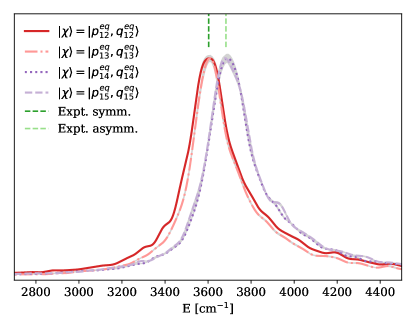
Figure 1: Semiclassical power spectra in the O-H stretching region, for different reference coherent states and corresponding trajectory sampling, as described in Sec. III.1. The straight dashed lines correspond to the experimental results of Ref. Hammer et al., 2005 for the (monomer) symmetric and (monomer) asymmetric bands. Gray bands behind the curves indicate the standard deviation of the estimated spectra.

In Fig. 1, we show the results for the fundamental O-H stretching modes. Experimentally, a doublet is observed.Hammer et al. (2005) MCTDH Vendrell, Gatti, and Meyer (2007b) indicated that each peak of the doublet comprises two fundamental states, and that the degeneracy of the lower energy peak is slightly lifted.

We consider the set of vibrational stretchings (modes $12-15$), and sample their initial momenta with the distribution in Eq. (18) centered at their ZPE momenta $p_{l}^{eq}=\sqrt{\omega_{l}}$. All other modes have initial null velocity. We employ antisymmetrized coherent states, of type (i), centered at the same momenta as the relevant reference states. These stretching modes are usually fairly decoupled from the rest of the dynamics, due to their high energy, in the $3000\div 4000~{}\text{cm}^{-1}$ range. We find very good agreement with both the MCTDH results and the experimental observations. We adopt the nomenclature of Ref. Pitsevich et al., 2017, $a(m)b(d)$, simplified into $a-b$, where $a=s,as$ and $b=s,as$. $s(m)$ and $as(m)$ indicate the symmetry/asymmetry of the monomer stretchings and $s(d)$, $as(d)$ indicate the in- or out-of-phase combination of the monomer stretchings in the dimer. The $s-as$ and $s-s$ modes are essentially degenerate. The optically active one ($s-as$), at $3607\text{cm}^{-1}$, is compatible with the experimental observation at $3603\text{cm}^{-1}$ and with the MCTDH result at $3607\text{cm}^{-1}$. The fully symmetric optically inactive mode ($s-s$), found at $3609\text{cm}^{-1}$, is compatible with the MCTDH result at $3614\text{cm}^{-1}$. For the higher frequency peak, which has double degeneracy and corresponds to the optically active monomer-asymmetric modes, we obtain two estimates, $3679\text{cm}^{-1}$ for $as-as$ and $3690\text{cm}^{-1}$ for $as-s$, that differ by only $\sim 10\text{cm}^{-1}$. They are equivalent within the uncertainty given by the finite number of trajectories and compare very well to the MCTDH result at $3689\text{cm}^{-1}$ and the experimental observation at $3683\text{cm}^{-1}$.

III.2 Bending modes

In Fig. 2, we show our results for the subspace of the two in-plane water bendings (normal modes $10,11$). We sample their momenta around the ZPE harmonic prescription $p_{l}^{eq}=\sqrt{\omega_{l}}$, together with the O-H stretching modes. The stretching modes are initialized at their ZPE momenta, while all other modes are initialized at zero momentum. We employ antisymmetrized coherent states of type (i) centered at the same momenta as the relevant reference states. We find very good agreement with MCTDH ($1741\text{cm}^{-1}$) and the experimental values ($1763\text{cm}^{-1}$) for the higher energy mode, found at $1751\text{cm}^{-1}$. This mode is optically active, because the corresponding normal mode contains a significant contribution from proton transfer. The lower frequency mode, at $1668\text{cm}^{-1}$, is not optically active, since the corresponding normal mode involving a perpendicular shared proton fluctuation, and we cannot thus compare it to experiment. Notice that the height of the power spectrum peak is arbitrarily normalized, and not directly comparable to absorption spectra. Our result is half way between the harmonic ($1720\text{cm}^{-1}$) and the MCTDH ($1606\text{cm}^{-1}$) ones.

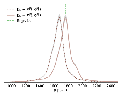
Figure 2: Semiclassical power spectra in the bendings’ region. Curves refer to different reference coherent states and trajectory sampling, as explained in Sec. III.2. The straight dashed line corresponds to the experimental result of Ref. Hammer et al., 2005 for optically active bending band. Gray bands behind the curves indicate the standard deviation of the estimated spectra.

III.3 Proton transfer modes

In Fig. 3, we show our results for the proton transfer excitation. Experimentally, the proton transfer mode shows a very neat doublet, especially when the protonated water dimer is tagged with Ne.Hammer et al. (2005) These two states have been investigated in many articles, due to their controversial nature.Kaledin, Kaledin, and Bowman (2006); Vendrell, Gatti, and Meyer (2007b); Vendrell and Meyer (2008) Initially, the doublet was associated to tunneling splitting similar to hydrogen bonding. However, it is now clear that, in most of the relevant configuration space close to equilibrium, the shared proton only visits a shallow single minimum (see Sec. III.6),Schran, Brieuc, and Marx (2018); Marx (2006) and the doublet structure is due to a Fermi resonance involving the bare proton-transfer mode and a combination of O-O stretching and wagging modes.Vendrell, Gatti, and Meyer (2007b, 2009b) Due to the very shallow shape of the PES in this region, this is a very tough calculation for a semiclassical approach, which relies of the evaluation of the Hessian matrix along classical trajectories. In Ref. Di Liberto, Conte, and Ceotto, 2018b, some of us proposed an interpretation in terms of a combination of the fundamental transition of the $7$-th mode (the bare proton transfer mode) and the first overtone of mode $3$ (namely, the second wagging mode). Here, we investigate more thoroughly this issue.

In the proton transfer dynamics, we identify three main players. One is the wagging normal mode $2$, which is per se a collective mode describing the out-of-phase combination of the monomer-localized wagging modes. In the notation of Ref. Vendrell, Gatti, and Meyer, 2007b, this state can be identified with $w_{3}$, namely an overtone in the wagging subspace. The second one is mode 7, which describes the bare proton transfer. By inspecting matrix $\bm{L}$, normal modes 7 and 2 are those which give the largest contribution to the projection of the shared proton on the O-O axis. In particular, both modes involve asymmetric wagging of the water monomers, synchronized with shared proton transfer, and they essentially differ by the sign and amplitude of the proton transfer component. The third relevant player is normal mode 6, describing O-O stretching, which couples very anharmonically to proton transfer.

To avoid too chaotic trajectory dynamics, we choose to sample the initial momentum of mode $7$ only, around its fundamental energy, $p_{7}^{eq}=\sqrt{3\omega_{7}}$. All the other modes are initialized at zero momentum, but obviously get excited along the trajectories because of the quick energy transfer. Other choices, in which the sampling subspace $\mathcal{S}^{\prime}$ is extended, would deteriorate the signal, since trajectories would soon become unstable and thus yield a broader spectrum. This refined methodology allows us to observe a clean spectral feature in the $800-1100\text{cm}^{-1}$ region, with two peaks at $891\text{cm}^{-1}$ and $1062\text{cm}^{-1}$, to be compared with the experimental doublet for the Ne-tagged molecule at $928\text{cm}^{-1}$ and $1047\text{cm}^{-1}$ and the MCTDH results at $918\text{cm}^{-1}$ and $1033\text{cm}^{-1}$.

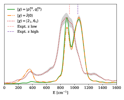
Figure 3: Semiclassical power spectra in the proton transfer region. Curves refer to different reference states, of types (i), (iii), and (ii), respectively. The corresponding trajectory sampling is described in Sec. III.3. The straight dashed lines correspond to the experimental result of Ref. Hammer et al., 2005 for the proton transfer doublet. Gray bands behind the curves indicate the standard deviation of the estimated spectra.

Now, we want to understand each mode contribution to the doublet peaks. For this goal, we employ three different reference states. The first one is the coherent state $\ket{\chi}=\ket{p_{7}^{eq},q_{7}^{eq}}$. Once properly antisymmetrized according to Eq. (13), it directly shows a neat doublet structure, where the higher frequency peak is very close to experiment, while the lower frequency peak is half way between the experimental peak and the harmonic $7_{1}$ excitation. Given the strongly chaotic nature of these modes dynamics, we observe the peak width to depend on the maximum number of time-steps of the trajectories. When choosing a looser $\epsilon$ threshold, the main contribution is given by few long-time trajectories and the Monte Carlo convergence for the higher frequency peak is very tough. Instead, if one chooses a smaller value of $\epsilon$, trajectories are too short to yield a well-resolved and accurate enough signal. For these reasons, the Monte Carlo uncertainty for the two peaks is$~{}\sim 30\text{cm}^{-1}$.

The second reference that we employ is the harmonic ground state, excited by the $z$ coordinate $\ket{\chi}=\hat{z}\ket{\bm{0}}$, evaluated as described in Sec. II.4 at iii). Since all normal modes contribute to the composition of this reference state, we can find a third peak at $358\text{cm}^{-1}$. We assign it to $w_{3}$, corroborating the view that the wagging mode is intimately linked to proton transfer.

The third reference state is of type (ii), namely the combined harmonic overtone of the wagging and the O-O stretching modes $\ket{\chi}=\ket{2_{1},6_{1}}$, indicated as $(w_{3},1R)$ in Ref. Vendrell, Gatti, and Meyer, 2007b. In this case, we modify the sampling subspace $\mathcal{S}^{\prime}$ and sample the initial momenta of the $2$nd and $6$th normal-modes around their harmonic approximations $p_{l}=\sqrt{\omega_{l}}$. The resulting semiclassical power spectrum manifests again a small feature at a frequency $~{}380\text{cm}^{-1}$, which can be assigned an uncertainty of $~{}\sim 25{cm}^{-1}$, and a very prominent peak situated in the region of the lower-energy peak of the proton-transfer doublet. Here, the Monte Carlo uncertainty is higher because of the slow convergence in the trajectory number due to the O-O stretching initial excitation. Then, it is reasonable to consider this peak as compatible with the lower frequency peak originated from the $\ket{\chi}=\ket{p_{7}^{eq},q_{7}^{eq}}$ spectrum and to infer a major contribution of the $(w_{3},1R)$ to the lower-energy peak.

III.4 Proton perpendicular modes

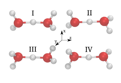
Figure 4: Four minima of the Zundel cation geometry that are relevant for the description of the perpendicular motion of the shared proton.

The vibrational states mainly describing the motion of the shared proton perpendicular to the O-O segment ($z$ direction) are conventionally called $x$ and $y$. In Fig. 4, we call version I the reference geometry minimum of the PES employed in this work. Such geometry minimum manifests $C_{2}$ symmetry, and the normal modes which mostly pertain to the shared-proton $x$ and $y$ states are the $9$th and the $8$th, corresponding to very different harmonic frequencies $\omega_{9}=1574\text{cm}^{-1}$ and $\omega_{8}=1494\text{cm}^{-1}$. However, for fluxional molecules, a single global minimum is not sufficient to describe the relevant symmetries, since very anharmonic low-frequency modes, like internal rotational modes (torsions and waggings), experience relatively low-energy barriers towards other equivalent global minima. These minima are related to the reference one by a combination of global rotations, reflections and permutations. For these systems, the relevant symmetry group is a permutation-inversion group, as introduced by Longuet-Higgins in Ref. Longuet-Higgins, 1963. The barrier for wagging is particularly small ($\sim 100\text{cm}^{-1}$),Wales (1999) and the Zundel cation belongs to the $\mathcal{G}_{16}$ group, once torsion and wagging of the water monomers are properly considered. Within this extended group, the $x$ and $y$ states must be degenerate, being of $E$ symmetry. This can be seen in Fig. 4, where we indicated by I, II, III, IV the four global minima of the molecule, that can be reached when $0$, $1$, or 2 monomer inversions (wagging) are considered (we do not consider the feasibility of overcoming the torsional barrier). In particular, version II is accessible via the right monomer wagging, version III via the left monomer wagging, version IV via both waggings. In terms of permutation-inversions, version II can be obtained by first a $-\pi/2$ rotation around the $z$-axis, then a reflection $x\to-x$ and finally the permutation of the hydrogens of the left monomer. Version III is instead obtained by a $\pi/2$ rotation around the $z$-axis, then a reflection $x\to-x$ and finally the permutation of the hydrogens of the right monomer. Version IV is obtained by a $\pi$ rotation around the $z$-axis and the permutation of both the left hydrogens and, separately, of the right hydrogens. We call these operations $\mathcal{P}_{A}$, where $A=$I, II, III, IV and $\mathcal{P}_{I}$ is the identity.

When viewed from versions II or III, the shared-proton $x$ motion is dominated by normal mode $8$, instead of $9$, at variance with versions I and IV. The opposite is true for the $y$ motion. By properly taking into account sign changes, we then introduce two symmetrized states of harmonic modes of the type (ii), that describe the perpendicular motion:

$$\ket{y_{S}}=\ket{8_{1}}_{\text{I}}+\ket{9_{1}}_{\text{II}}-\ket{9_{1}}_{\text{III}}-\ket{8_{1}}_{\text{IV}}$$ (20)

and

$$\ket{x_{S}}=\ket{9_{1}}_{\text{I}}-\ket{8_{1}}_{\text{II}}+\ket{8_{1}}_{\text{III}}-\ket{9_{1}}_{\text{IV}}$$ (21)

where the indexes I, II, III, IV indicate in which geometry the normal modes are defined. Equivalently, one may make linear combinations of properly antisymmetrized coherent states of type (i). The two states are linearly independent, and have the same energy, since one can apply the operators $\mathcal{P}_{A}$, which commute with the Hamiltonian, to convert one into the other.

According to MCTDH estimates, the energy of the proton-perpendicular subspace is $1391\text{cm}^{-1}$. If we naively sampled separately normal modes $8$ and $9$, only referred to version I and with momenta centered at their respective first excited harmonic energies, we would obtain non-degenerate peaks, although strongly red-shifted from the harmonic values.

The correct procedure is, on the contrary, to enforce the described symmetry and consider the reference states $\ket{y_{S}}$ and $\ket{x_{S}}$. Moreover, also the sampling of trajectories is to be symmetrized, in principle by launching ensembles of trajectories starting from the four versions of the molecule and with the momentum of the shared proton in the $x$ direction.Conte, Aspuru-Guzik, and Ceotto (2013) However, a more efficient procedure exploits the symmetry operations $\mathcal{P}_{A}$, by sampling trajectories centered on version I only, but by summing the contributions of 4 different samples of momenta: two centered on the fundamental excitation of mode $8$, but with opposite signs, and two centered on the fundamental excitation of mode $9$, with both signs, for a total of $96000$ trajectories. To better explore the regions of phase space close to monomer inversions, we also give initial momentum to the other normal modes which facilitate such motions, namely to modes 2 and 7, with an energy corresponding to their harmonic ZPE. Moreover, the calculation of the overlap between the running coherent states and the reference states $\ket{y_{S}}$ and $\ket{x_{S}}$ may use the relations $\langle\bm{x}|8_{1}\rangle_{A}=\langle\mathcal{P}_{A}^{-1}(\bm{x})|8_{1}\rangle_{I}$ that relate the Cartesian coordinates referred to geometry A to the coordinates referred to geometry I by using the inverse operators $\mathcal{P}_{A}^{-1}$. The resulting spectra are showed in Fig. 5. One can see that degeneracy for the main peaks is essentially recovered, within errorbars, and that the semiclassical estimate for the perpendicular states is $1453\text{cm}^{-1}$, given by the average value of the two spectral peaks. We are unable to assign the minor features that appear far from the main peaks, due to insufficient trajectory sampling in that region.

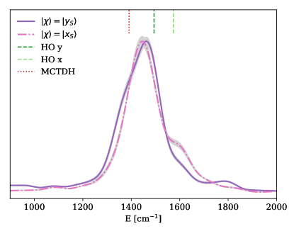
Figure 5: Semiclassical power spectra in the shared proton perpendicular mode region, employing symmetrized reference states of type (iv) and multi-reference trajectory sampling, as explained in Sec. III.4. The straight dashed lines correspond to the non degenerate harmonic frequencies of the 8th and 9th normal modes. The dotted line indicates the MCTDH result from Ref. Vendrell, Gatti, and Meyer, 2007b . Gray bands behind the curves indicate the standard deviation of the estimated spectra.

III.5 O-O stretching related states

We now perform our TA SCIVR calculation for the strong anharmonic modes involving the O-O stretching. In Fig. 6, we report the power spectra of the harmonic states $\ket{6_{1}}$ and $\ket{6_{2}}$, namely those containing one or two excitations of $R$, according to Ref. Vendrell, Gatti, and Meyer, 2007b nomenclature. We employ a subspace $\mathcal{S}^{\prime}$ momentum sampling involving normal modes $2$ (wagging), $6$ (O-O stretch), and $7$ (proton transfer). We sample modes $6$ and $7$ by centering the distribution of their momenta around their fundamental energies. Mode $2$ is also sampled, around its ZPE-associated momentum, because of its strong coupling to both other states. We noticed, indeed, that especially the estimation of the correlated state $1R$ is influenced by the sampling of mode $2$. However, exciting the wagging and the O-O stretching modes together results in strongly chaotic trajectories. This implies an amplified Fourier uncertainty of $60\text{cm}^{-1}$. Thus, for these spectra, we employ $34000$ trajectories. The relatively large statistical uncertainties present in Fig. 6 indicate the slow convergence due to the strong anharmonicity of these modes. We did not pursue calculations with even more trajectories, given the expected uncertainty due to the Fourier transform. However, we notice a good estimate of the $1R$ frequency at $580\text{cm}^{-1}$, to be compared to the MCTDH result at $550\text{cm}^{-1}$, and an acceptable evaluation of the $2R$ frequency at $1124\text{cm}^{-1}$, which is strongly red-shifted from the harmonic expectation, but partially blue-shifted with respect to the MCTDH calculation, at $1069\text{cm}^{-1}$.

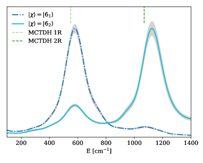
Figure 6: Semiclassical power spectra in the O-O stretching region, employing harmonic reference states of type (ii), and trajectory sampling as explained in Sec. III.5. The straight dashed lines indicate the MCTDH results from Ref. Vendrell, Gatti, and Meyer, 2007b. Gray bands behind the curves show the standard deviation of the estimated spectra.

III.6 Insight from single trajectories

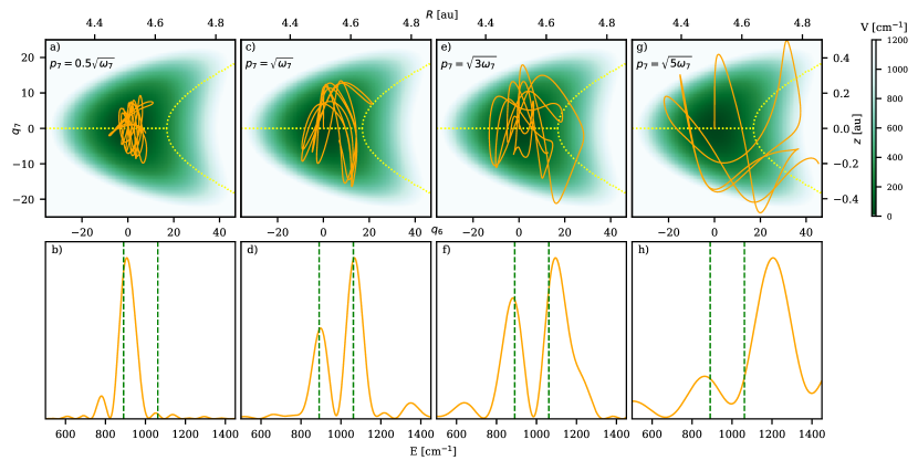
Figure 7: Upper panels: density plot of a section of the PES with all normal modes set to equilibrium except for modes $q_{6}$ (O-O stretching) and $q_{7}$ (proton transfer); top and right axes show the corresponding $R$ and $z$ coordinates; for each value of $q_{6}$, the minima of the PES with varying $q_{7}$ are indicated (dotted lines); the projections of the trajectories, where only $p_{7}$ is initially excited, are indicated (solid line). Lower panels: corresponding single trajectory spectra from Eq. (19) employing the $\ket{p_{7}^{eq},q_{7}^{eq}}$ reference state; the position of the peaks from phase-space integration (Table 1) is indicated (dashed lines).

One may ask to what extent single classical trajectories are informative of the quantum dynamics of the system, in the spirit of the MC SCIVR approach.Ceotto et al. (2009b) For example, tunneling splitting in ammonia has been resolved with few trajectories.Conte, Aspuru-Guzik, and Ceotto (2013) Here, we focus on the proton transfer mode, and deepen our investigation on the role of possible tunneling splitting versus anharmonicity.

We give initial kinetic energy only to the 7-th normal mode, varying its initial momentum, while setting all the initial coordinates at the reference geometry. In Fig. 7, we observe that some single trajectories yield the expected doublet spectral structure, and that this feature strongly and quantitatively depends on the initial $p_{7}$ momentum. To gain more physical insight, we draw the projection of the trajectories onto the subspace spanned by modes 7 (proton transfer) and 6 (O-O stretching), which are close enough to the global minimum and essentially dominated by the coordinates $z=x_{H,z}-(x_{O_{1},z}+x_{O_{2},z})/2$ and $R=x_{O_{2},z}-x_{O_{1},z}$. We also draw the corresponding section of the PES (when all other normal modes are kept at equilibrium), and indicate the minimum of the PES along the proton transfer direction, with varying $R$ distance. One can see that, only for $R\gtrsim 4.63a.u.$, a double minimum shape is acquired by the potential restricted to the $q_{7}$ coordinate. When $p_{7}\ll\sqrt{\omega_{7}}$ (panels a,b), the trajectory does not leave the shallow global well and a single peak appears in the spectrum, close to the harmonic result, because only the bottom of the well is sampled. For $p_{7}=\sqrt{\omega_{7}}$ (panels c,d), a double-peak structure is obtained, which is surprisingly close to the integrated spectrum, even though the trajectory seems to be mostly confined to the region where a single well is present. This is consistent with the already discussed interpretation of the doublet as arising not from tunneling, but from strong anharmonicity and coupling to O-O stretching (for simplicity, we do not discuss here the wagging coordinate).Schran, Brieuc, and Marx (2018) Notice, also, that here we have used a single reference coherent state centered at the geometry minimum, so the coherent states following each classical trajectory are not overlapping with a superposition of localized states, differently than the case of ammonia of Ref. Conte, Aspuru-Guzik, and Ceotto, 2013.

For higher momentum $p_{7}=\sqrt{3\omega_{7}}$ (panels e,f), corresponding to the center of the sampling described in Sec. III.3, a small part of the trajectory is indeed exploring the double-well region. The doublet is still present, but the trajectory is apparently less recurring on already visited space, probably due to excitation of many other coordinates (not visible in the projection). At even higher initial momentum (panels g,h), energy transfer is so high that the resulting spectrum is quite broadened and the doublet is essentially lost. Notice that the integrated spectra showed in Sec. III.3 contain all these contributions, properly weighted by the reference state.

We draw again the conclusion that the double-well structure, and a related tunneling splitting, is not relevant in quantitatively explaining the proton-transfer doublet. An extensive analysis of the delocalization of the shared proton as a function of the relative O-O distance has been recently performed using path-integral methods.Schran, Brieuc, and Marx (2018)

IV Conclusions

In this work, we tackled the challenging problem of the estimation of the vibrational spectrum of a strongly anharmonic molecule, such as the protonated water dimer, by means of a TA SCIVR method. We showed that it is currently possible to reach a $20\text{cm}^{-1}$ spectroscopic accuracy, similarly to what has already been established for smaller molecules. The crucial improvements, that rendered this calculation possible, are: (i) the analytical definition of global translational and rotational coordinates at equilibrium; (ii) the accounting for the contribution of all classical trajectories, with a weight depending on the duration of their stability; (iii) the application of various reference states, highlighting the nature of the states of interest; (iv) the tailored initial distribution of kinetic energy to the modes that form the subspaces of the DC approach, avoiding the initial excitation of floppy modes, and (v) the proper symmetrization of both the reference state and trajectory sampling, when dealing with the full symmetry group of fluxional molecules.

We believe this work paves the way toward different research directions. In particular, due to the strongly anharmonic nature of acid solutions, and of water clusters, integration over phase space of at least some relevant modes is probably necessary to obtain valuable quantitative, and not only qualitative, comparison to the experimental results. To be competitive, phase-space integration necessitates high-dimensional PES. Nevertheless, as the analysis of the proton transfer mechanism demonstrates, valuable qualitative information can be extracted also from a single suitably chosen trajectory, and this should be investigated more. Moreover, the chaotic nature of most of the trajectories stimulates an effort in extracting useful information from short time duration, employing estimation techniques other than the Fourier transform, that allow to reduce the width of the reconstructed spectral peaks by means of, for example, filter diagonalization, compressed sensing or super-resolution. The floppiness of water complexes points at the usefulness of an Eckart frame in defining normal modes in regions far from the equilibrium geometryWehrle, Šulc, and Vaníček (2014) and to a proper consideration of multiple geometries in the reference states. The divide-and-conquer approach adopted for the phase space integration showed a reasonable scaling respect to number of degrees of freedom and it opens the route for tackling higher dimension protonated water clusters. Finally, since an electric dipole surface is available from Ref. Huang, Braams, and Bowman, 2005, the evaluation of the full absorption spectrum should be feasible.Micciarelli et al. (2018, 2019)

Appendix A Properties of coherent states

From now on, we assume that the quantum numbers associated to global translational and rotational invariance, namely the momentum of the center of mass and the angular momentum, are set to zero.

The remaining $\tilde{F}$ normal modes’ coordinates are promoted to operators $\hat{q}_{l}$ and $\hat{p}_{l}$, respecting the canonical commutation relations $\left[\hat{q}_{l},\hat{p}_{l^{\prime}}\right]=i\delta_{ll^{\prime}}$. Let us introduce the annihilation and construction operators via $\hat{a}_{l}=\frac{1}{\sqrt{2}}\left(\sqrt{\omega_{l}}\hat{q}_{l}+\frac{i}{\sqrt{w_{l}}}\hat{p}_{l}\right)$ and $\hat{a}_{l}^{\dagger}=\frac{1}{\sqrt{2}}\left(\sqrt{\omega_{l}}\hat{q}_{l}-\frac{i}{\sqrt{w_{l}}}\hat{p}_{l}\right)$, where $\left[\hat{a}_{l},\hat{a}_{l^{\prime}}^{\dagger}\right]=1$. The harmonic vacuum state for a single normal mode $\ket{0}$ is defined by $\hat{a}_{l}\ket{0}=0$, and has coordinate representation $\braket{q_{l}}{0}=(\omega/\pi)^{1/4}\exp{(-\omega q_{l}^{2}/2)}$.

Two classes of states are of major importance in the context of semiclassical vibrational spectroscopy: harmonic states and coherent states. The normalized harmonic basis is defined by the repeated action of the creation operator $\ket{l_{n}}=\frac{(\hat{a}_{l}^{\dagger})^{n}}{\sqrt{n!}}\ket{0}$, with the property that $\ket{l_{n}}$ is the eigenvector of the number operator $\hat{N}_{l}=\hat{a}_{l}^{\dagger}\hat{a}_{l}$ with eigenvalue $n$. To account for harmonic excitations of different normal modes, tensor products are formed $\ket{1_{n_{1}},2_{n_{2}},\dots,\tilde{F}_{n_{\tilde{F}}}}\equiv\ket{1_{n_{1}}}\ket{2_{n_{2}}}\dots\ket{\tilde{F}_{n_{\tilde{F}}}}$.

The coherent states are defined to be eigenvectors of the destruction operator (we omit now the normal mode index $l$ for clarity) $\hat{a}\ket{\alpha}=\alpha\ket{\alpha}$, where $\alpha$ is a complex number, which is uniquely defined by the expectation values of position $q^{\alpha}\equiv\braket{\alpha}{\hat{q}}{\alpha}=\braket{\alpha}{\frac{\hat{a}+\hat{a}^{\dagger}}{\sqrt{2\omega}}}{\alpha}=\frac{\alpha+\alpha^{*}}{\sqrt{2\omega}}=\Re{(\alpha)}\sqrt{\frac{2}{\omega}}$ and momentum $p^{\alpha}\equiv\braket{\alpha}{\hat{p}}{\alpha}=\braket{\alpha}{\frac{\hat{a}-\hat{a}^{\dagger}}{i}{\sqrt{\frac{\omega}{2}}}}{\alpha}=\frac{\alpha-\alpha^{*}}{i}{\sqrt{\frac{\omega}{2}}}=\Im{(\alpha)}\sqrt{2\omega}$. Thus $\alpha\equiv\frac{1}{\sqrt{2}}\left(\sqrt{\omega}q^{\alpha}+\frac{i}{\sqrt{w}}p^{\alpha}\right)$. Typically, when $\omega$ is clear from the context, we also denote $\ket{\alpha}=\ket{p^{\alpha},q^{\alpha}}$.

To obtain the expansion of coherent states in the harmonic basis $\ket{\alpha}=\sum_{n=0}^{\infty}c_{n}\ket{n}$ (where again, we omit the normal mode index $l$ and only indicate the number of harmonic excitations $n$), we notice that $\braket{n}{\alpha}=\braket{0}{\frac{\hat{a}^{n}}{\sqrt{n!}}}{\alpha}=\frac{\alpha^{n}}{\sqrt{n!}}\braket{0}{\alpha}=c_{0}\frac{\alpha^{n}}{\sqrt{n!}}$. To fix the modulus of $c_{0}$, one evaluates the norm $\braket{\alpha}{\alpha}=\sum_{n=0}^{\infty}|c_{n}|^{2}=|c_{0}|^{2}\sum_{n=0}^{\infty}\frac{|\alpha|^{2n}}{n!}=|c_{0}|^{2}e^{|\alpha|^{2}}\equiv 1$. Therefore, one gets the well-known relation:

$$\ket{\alpha}=e^{-|\alpha|^{2}/2}e^{-i\frac{p^{\alpha}q^{\alpha}}{2}}\sum_{n=0}^{\infty}\frac{\alpha^{n}}{\sqrt{n!}}\ket{n}\;,$$ (22)

where the arbitrary global complex phase, which is relevant when taking overlaps of different states, is fixed by adopting the convention widely used in the context of the semiclassical literature. By using the Baker-Campbell-Hausdorff formula $\exp{(\hat{A}+\hat{B})}=\exp{(\hat{A})}\exp{(\hat{B})}\exp{(-c/2)}$, provided $\left[\hat{A},\hat{B}\right]=c$ is a C-number, it is easy to verify that the above equation is equivalent to the standard relation

$$\ket{\alpha}=e^{-i\frac{p^{\alpha}q^{\alpha}}{2}}e^{\alpha\hat{a}^{\dagger}-\alpha^{*}\hat{a}}\ket{0}=e^{-iq^{\alpha}\hat{p}}e^{i\hat{q}p^{\alpha}}\ket{0}\;.$$ (23)

The coordinate representation of a coherent state is thus:

$$\braket{q}{\alpha} =\braket{q}{e^{-iq^{\alpha}\hat{p}}e^{i\hat{q}p^{\alpha}}}{0}=\braket{q-q^{\alpha}}{e^{i\hat{q}p^{\alpha}}}{0}$$

$$=e^{i(q-q^{\alpha})p^{\alpha}}\braket{q-q^{\alpha}}{0}$$

$$=\left(\frac{\omega}{\pi}\right)^{\frac{1}{4}}e^{-\frac{\omega}{2}(q-q^{\alpha})^{2}+ip^{\alpha}(q-q^{\alpha})}$$ (24)

having used $e^{iq^{\alpha}\hat{p}}\ket{q}=\ket{q-q^{\alpha}}$.

The overlap of two coherent states is:

$$\braket{\alpha}{\beta} =e^{-\frac{|\alpha|^{2}+|\beta|^{2}}{2}+i\frac{p^{\alpha}q^{\alpha}-p^{\beta}q^{\beta}}{2}}\sum_{n,n^{\prime}=0}^{\infty}\frac{(\alpha^{*})^{n}\beta^{n^{\prime}}}{\sqrt{n!n^{\prime}!}}\braket{n}{n^{\prime}}$$

$$=e^{-\frac{|\alpha|^{2}+|\beta|^{2}}{2}+i\frac{p^{\alpha}q^{\alpha}-p^{\beta}q^{\beta}}{2}}\sum_{n=0}^{\infty}\frac{(\alpha^{*}\beta)^{n}}{n!}$$

$$=e^{\alpha^{*}\beta-\frac{|\alpha|^{2}+|\beta|^{2}}{2}+i\frac{p^{\alpha}q^{\alpha}-p^{\beta}q^{\beta}}{2}}$$

$$=e^{-\frac{\omega(q^{\alpha}-q^{\beta})^{2}}{4}-\frac{(p^{\alpha}-p^{\beta})^{2}}{4\omega}+i\frac{(p^{\alpha}+p^{\beta})(q^{\alpha}-q^{\beta})}{2}}\;.$$ (25)

It is particularly easy to calculate the expectation value of creation and destruction operators in coherent states:

$$\braket{\alpha}{(\hat{a}^{\dagger})^{n}}{\beta}=(\alpha^{*})^{n}\braket{\alpha}{\beta},\quad\braket{\alpha}{\hat{a}^{n}}{\beta}=\beta^{n}\braket{\alpha}{\beta}.$$ (26)

In the calculation of some of the semiclassical survival amplitudes evaluated in this work, the expectation value of a normal mode coordinate operator is relevant:

$$\braket{\alpha}{\hat{q}}{\beta} =\frac{\braket{\alpha}{\hat{a}+\hat{a}^{\dagger}}{\beta}}{\sqrt{2\omega}}=\frac{\beta+\alpha^{*}}{\sqrt{2\omega}}\braket{\alpha}{\beta}$$

$$=\left(\frac{q^{\alpha}+q^{\beta}}{2}-i\frac{p^{\alpha}-p^{\beta}}{2\omega}\right)\braket{\alpha}{\beta}\;.$$ (27)

Notice that in the MC SCIVR approach,Ceotto et al. (2009b) emphasis on specific modes is put by considering coherent overlaps of the form:

$$\bra{\alpha} \left(\ket{p^{\beta},q^{\beta}}-\ket{-p^{\beta},q^{\beta}}\right)=\bra{\alpha}\left(\ket{\beta}-\ket{\beta^{*}}\right)$$

$$=e^{-\frac{\omega(q^{\alpha}-q^{\beta})^{2}}{4}-\frac{(p^{\alpha}-p^{\beta})^{2}}{4\omega}+i\frac{(p^{\alpha}+p^{\beta})(q^{\alpha}-q^{\beta})}{2}}$$

$$\phantom{=}-e^{-\frac{\omega(q^{\alpha}-q^{\beta})^{2}}{4}-\frac{(p^{\alpha}+p^{\beta})^{2}}{4\omega}+i\frac{(p^{\alpha}-p^{\beta})(q^{\alpha}-q^{\beta})}{2}}$$

$$=\braket{\alpha}{\beta}\left(1-e^{-\frac{p^{\alpha}p^{\beta}}{\omega}-ip^{\beta}(q^{\alpha}-q^{\beta})}\right)$$

$$\underset{p^{\beta}\to 0}{\sim}2ip^{\beta}\braket{\alpha}{\beta}\left(\frac{q^{\alpha}-q^{\beta}}{2}-i\frac{p^{\alpha}}{2\omega}\right)\;,$$ (28)

which is proportional to Eq. (27), provided momentum $p^{\beta}$ is small and the center of the reference state is $q^{\beta}=0$.

Finally, the expectation value of a Cartesian coordinate operator, considering the relevant case $\ket{\bm{\beta}}=\ket{\bm{0}}$, is simply given by a linear combination of normal modes’ expectation values:

$$\braket{\bm{\alpha}}{\hat{x}_{j\gamma}}{\bm{0}}-{x}_{j\gamma}^{eq}=\braket{\bm{\alpha}}{\bm{0}}\sum_{l}\frac{L_{j\gamma,l}}{\sqrt{m_{j}}}\left[\frac{(q^{\alpha})_{l}}{2}-i\frac{(p^{\alpha})_{l}}{2\omega}\right].$$ (29)

Appendix B Global translational and rotational symmetries

We follow Refs. Eckart, 1935; Wilson, Decius, and Cross, 1980; Miller, Handy, and Adams, 1980; Jellinek and Li, 1989 in analytically defining the normal modes corresponding to global translations and infinitesimal rotations at the reference geometry.

We proceed with a classical derivation using Poisson brackets, which can easily translated to quantum formalism. We generically consider a function which is a linear superposition of single atom (mass-scaled) Cartesian momenta:

$$B=\sum_{k\beta}b_{k\beta}(\bm{X})P_{k\beta}\;,$$ (30)

where, possibly, the coefficients $b_{k\beta}$ depend on the position, and we render the axis coordinate $\beta$ explicit. We assume that the Poisson bracket of such function with the interaction potential is zero: $\{B,V(\bm{X})\}=0$. Since the interaction potential does not depend on momentum, we get

$$\sum_{k\beta}b_{k\beta}(\bm{X})\frac{\partial V}{\partial X_{k\beta}}=0\;,$$ (31)

namely, functions, which are linear combinations of momenta and have null Poisson bracket (commute) with the interaction potential, simply correspond to null gradients of the potential along the same linear combinations of Cartesian coordinates.

From the above commutation relation, it obviously follows that $\{B,\{B,V(\bm{X})\}\}=0$. We thus get:

$$\sum_{k\beta,j\alpha}\left(b_{k\beta}(\bm{X})\frac{\partial b_{j\alpha}(\bm{X})}{\partial X_{k\beta}}\frac{\partial V}{\partial X_{j\alpha}}+\right.\\ \left.b_{k\beta}(\bm{X})b_{j\alpha}(\bm{X})\frac{\partial^{2}V}{\partial X_{k\beta}\partial X_{j\alpha}}\right)=0\;.$$ (32)

In the case of global momentum, associated to the translational symmetry of the molecule as a whole, $\partial b_{j\alpha}/\partial X_{k\beta}=0$. So, it is guaranteed that also the second derivative of the potential along the direction corresponding to $\bm{b}$, at any position, is null, since the first term in Eq. (32) drops out. In order to analytically assign such zero eigenvalues to global translations, we explicitly construct the corresponding eigenvectors and conventionally associate them to the last three rows of $\bm{L}^{T}$. Since the (not mass-scaled) center-of-mass momenta of the molecule are $P_{\alpha}^{CM}={\sum_{k}\sqrt{m_{k}}P_{k\alpha}}$, we impose $p_{F-3+\alpha}=\sum_{k\beta}L_{F-3+\alpha,k\beta}^{T}P_{k\beta}\propto P_{\alpha}^{CM}$, yielding Eq. (7). It is clear that these vectors are orthonormal to each other. These rows of $\bm{L}^{T}$ do not depend on $\bm{X}^{eq}$, so they are independent of the initial position and orientation of the molecule. Their treatment is therefore analytical.

Rotation around any axis does not change the interaction potential, however it is beneficial to relate the normal coordinates corresponding to global rotations to the infinitesimal generators of rotation around the principal axes of inertia, namely the global angular momentum components. To render $\bm{L}$ more sparse, it is useful to use the principal axes’ coordinate frame. The inertia tensor of the reference geometry

$$\tilde{I}_{\alpha\beta}=\sum_{k}m_{k}\left[-x_{k\alpha}^{eq}x_{k\beta}^{eq}+\delta_{\alpha\beta}\sum_{\gamma}(x_{k\gamma}^{eq})^{2}\right]$$ (33)

is diagonalized with $\tilde{\bm{I}}=\bm{R}\bm{I}\bm{R}^{T}$, and the orthogonal matrix $\bm{R}$ is used to rotate the coordinates of the reference geometry to the principal axes’ frame of the reference geometry $\bm{X}_{i}^{eq}\to\bm{R}^{T}\bm{X}_{i}^{eq}$, which we then use throughout this article.

Global angular momentum is defined as

$$J_{\alpha}=\hbar\sum_{k\beta\gamma}\epsilon_{\alpha\gamma\beta}X_{k\gamma}P_{k\beta}\;,$$ (34)

where $\epsilon_{\alpha\gamma\beta}$ is the Levi-Civita symbol and $\hbar$ appears due to our definition of mass-scaled coordinates. In this case the linear coefficients

$$b_{k\beta}(\bm{X})=\hbar\sum_{\gamma}\epsilon_{\alpha\gamma\beta}X_{k\gamma}$$ (35)

do depend on position. So the first term in Eq. (32) is in principle not negligible, unless Eq. (32) is evaluated exactly at a stationary point of the potential.Miller, Handy, and Adams (1980) This is what is usually done when considering the equilibrium geometry. However, it is clear that numerical inaccuracy in calculating $\bm{X}^{eq}$ directly impacts the numerical determination of the rotational modes, namely, null or almost null eigenvalues of the Hessian, besides those corresponding to translations, do not necessarily accurately correspond to global rotations. On the contrary, rotational modes can and should be analytically determined independently of the evaluated Hessian. Ideally, one would also evaluate instantaneous rotational and vibrational modes all along the classical trajectories, especially when considering finite angular momentum or reaction dynamics,Eckart (1935); Miller, Handy, and Adams (1980); Peslherbe and Hase (1994) but we prefer to define a constant $\bm{L}$ matrix, and make the approximation of using the reference geometry coordinates instead of the instantaneous position coordinates $\bm{X}\to\bm{X}^{eq}$ in Eq. (34). Therefore, the introduced rotational modes are the exact infinitesimal rotations at the reference geometry.Wilson, Decius, and Cross (1980) The use of a fixed $\bm{L}$ is probably part of the reason why we are unable to faithfully discriminate the very low energy floppy modes. On the contrary, the relatively higher energy modes can be correctly assigned, since their harmonic widths are smaller and thus their typical classical motion is close to the geometry minimum. Nevertheless, the overlap factors quench the part of the classical motion which explores regions further from the geometry minimum.

We conventionally assign the penultimate three (two, for linear reference geometries) rows $\bm{L}^{T}$ to the rotational modes $p_{F-6+\alpha}=\sum_{k\beta}L_{F-6+\alpha,k\beta}^{T}P_{k\beta}$, and use Eqs. (30) and (35), to obtain $p_{F-6+\alpha}\propto\sum_{k\beta\gamma}\epsilon_{\alpha\gamma\beta}X_{k\gamma}^{eq}P_{i\beta}$ which implies Eq. (8), whose denominator simply guarantees normalization. The 9 scalar products of the infinitesimal rotation modes yield the inertia tensor, so orthogonality of those vectors is guaranteed when using the principal axes frame. Finally, the translational and rotational vectors are trivially orthogonal.

The above defined analytical translational and rotational modes are then projected away from all the internal vibrational modes, as obtained from the diagonalization of the scaled Hessian, via a Gram-Schmidt procedure. In the divide-and-conquer approach the rotational modes are disregarded (set to null values), and this is equivalent to make the approximations $\sum_{k\gamma\beta}\epsilon_{\alpha\gamma\beta}X_{k\gamma}^{eq}\delta X_{k\beta}\approx 0$ ($\alpha=1,2,3$). These equations resemble the Eckart conditions, with the difference that we do not use them to optimally rotate the reference frame at each step of the trajectories.Eckart (1935); Wehrle, Šulc, and Vaníček (2014); Wehrle, Oberli, and Vaníček (2015) When considering rovibrational spectra, on the contrary, using the Eckart frame would be crucial.

References

- Bowman, Carrington, and Meyer (2008) J. M. Bowman, T. Carrington, and H.-D. Meyer, Molecular Physics 106, 2145 (2008).
- Thomas and Carrington Jr (2015) P. S. Thomas and T. Carrington Jr, J. Phys. Chem. A 119, 13074 (2015).
- Bertaina, Galli, and Vitali (2017) G. Bertaina, D. E. Galli, and E. Vitali, Adv. Phys. X 2, 302 (2017).
- Miller (2001) W. H. Miller, J. Phys. Chem. A 105, 2942 (2001).
- Miller (2005) W. H. Miller, Proc. Natl. Acad. Sci. USA 102, 6660 (2005).
- Yang et al. (2019) N. Yang, C. H. Duong, P. J. Kelleher, A. B. McCoy, and M. A. Johnson, Science 364, 275 (2019).
- Gabas et al. (2018) F. Gabas, G. Di Liberto, R. Conte, and M. Ceotto, Chem. Sci. 9, 7894 (2018).
- Di Liberto, Conte, and Ceotto (2018a) G. Di Liberto, R. Conte, and M. Ceotto, J. Chem. Phys. 148, 104302 (2018a).
- Zundel and Metzger (1968) G. Zundel and H. Metzger, Z. Phys. Chem. 58, 225 (1968).
- Wales (1999) D. J. Wales, J. Chem. Phys. 110, 10403 (1999).
- Miyazaki et al. (2004) M. Miyazaki, A. Fujii, T. Ebata, and N. Mikami, Science 304, 1134 (2004).
- Shin et al. (2004) J.-W. Shin, N. I. Hammer, E. G. Diken, M. A. Johnson, R. S. Walters, T. D. Jaeger, M. A. Duncan, R. A. Christie, and K. D. Jordan, Science 304, 1137 (2004).
- Douberly et al. (2010) G. Douberly, R. Walters, J. Cui, K. D. Jordan, and M. Duncan, J. Phys. Chem. A 114, 4570 (2010).
- Thämer et al. (2015) M. Thämer, L. De Marco, K. Ramasesha, A. Mandal, and A. Tokmakoff, Science 350, 78 (2015).
- Wolke et al. (2016) C. T. Wolke, J. A. Fournier, L. C. Dzugan, M. R. Fagiani, T. T. Odbadrakh, H. Knorke, K. D. Jordan, A. B. McCoy, K. R. Asmis, and M. A. Johnson, Science 354, 1131 (2016).
- Fagiani et al. (2016) M. R. Fagiani, H. Knorke, T. K. Esser, N. Heine, C. T. Wolke, S. Gewinner, W. Schöllkopf, M.-P. Gaigeot, R. Spezia, M. A. Johnson, and K. R. Asmis, Phys. Chem. Chem. Phys. 18, 26743 (2016).
- Singh et al. (2006) N. J. Singh, M. Park, S. K. Min, S. B. Suh, and K. S. Kim, Angew. Chem. Int. Ed. 45, 3795 (2006).
- Agostini, Vuilleumier, and Ciccotti (2011) F. Agostini, R. Vuilleumier, and G. Ciccotti, J. Chem. Phys. 134, 084302 (2011).
- Yu and Bowman (2017) Q. Yu and J. M. Bowman, J. Am. Chem. Soc. 139, 10984 (2017).
- Yu and Bowman (2019) Q. Yu and J. M. Bowman, J. Phys. Chem. A 123, 1399 (2019).
- Egan and Paesani (2019) C. K. Egan and F. Paesani, J. Chem. Theory Comput. (2019), 10.1021/acs.jctc.9b00418.
- de Grotthuss (1806) C. J. T. de Grotthuss, Annales de chimie 58, 54 (1806).
- Agmon (1995) N. Agmon, Chem. Phys. Lett. 244, 456 (1995).
- Tuckerman et al. (1995) M. Tuckerman, K. Laasonen, M. Sprik, and M. Parrinello, J. Chem. Phys. 103, 150 (1995).
- Mohammed et al. (2005) O. F. Mohammed, D. Pines, J. Dreyer, E. Pines, and E. T. J. Nibbering, Science 310, 83 (2005).
- Marx (2006) D. Marx, Chem. Phys. Chem. 7, 1848 (2006).
- Berkelbach, Lee, and Tuckerman (2009) T. C. Berkelbach, H.-S. Lee, and M. E. Tuckerman, Phys. Rev. Lett. 103, 238302 (2009).
- Asmis et al. (2003) K. R. Asmis, N. L. Pivonka, G. Santambrogio, M. Brümmer, C. Kaposta, D. M. Neumark, and L. Wöste, Science 299, 1375 (2003).
- Fridgen et al. (2004) T. D. Fridgen, T. B. McMahon, L. MacAleese, J. Lemaire, and P. Maitre, J. Phys. Chem. A 108, 9008 (2004).
- Yeh et al. (1989) L. I. Yeh, M. Okumura, J. D. Myers, J. M. Price, and Y. T. Lee, J. Chem. Phys. 91, 7319 (1989).
- Headrick, Bopp, and Johnson (2004) J. M. Headrick, J. C. Bopp, and M. A. Johnson, J. Chem. Phys. 121, 11523 (2004).
- Hammer et al. (2005) N. I. Hammer, E. G. Diken, J. R. Roscioli, M. A. Johnson, E. M. Myshakin, K. D. Jordan, A. B. McCoy, X. Huang, J. M. Bowman, and S. Carter, J. Chem. Phys. 122, 244301 (2005).
- Huang, Braams, and Bowman (2005) X. Huang, B. J. Braams, and J. M. Bowman, J. Chem. Phys. 122, 044308 (2005).
- Dai et al. (2003) J. Dai, Z. Bačić, X. Huang, S. Carter, and J. M. Bowman, J. Chem. Phys. 119, 6571 (2003).
- McCoy et al. (2005) A. B. McCoy, X. Huang, S. Carter, M. Y. Landeweer, and J. M. Bowman, J. Chem. Phys. 122, 061101 (2005).
- Kaledin, Kaledin, and Bowman (2006) M. Kaledin, A. L. Kaledin, and J. M. Bowman, J. Phys. Chem. A 110, 2933 (2006).
- Kaledin et al. (2009) M. Kaledin, A. L. Kaledin, J. M. Bowman, J. Ding, and K. D. Jordan, J. Phys. Chem. A 113, 7671 (2009).
- Huang, Habershon, and Bowman (2008) X. Huang, S. Habershon, and J. M. Bowman, Chem. Phys. Lett. 450, 253 (2008).
- Rossi, Ceriotti, and Manolopoulos (2014) M. Rossi, M. Ceriotti, and D. E. Manolopoulos, J. Chem. Phys. 140, 234116 (2014).
- Rossi, Kapil, and Ceriotti (2017) M. Rossi, V. Kapil, and M. Ceriotti, J. Chem. Phys. 148, 102301 (2017).
- Di Liberto, Conte, and Ceotto (2018b) G. Di Liberto, R. Conte, and M. Ceotto, J. Chem. Phys. 148, 014307 (2018b).
- Vendrell et al. (2007) O. Vendrell, F. Gatti, D. Lauvergnat, and H.-D. Meyer, J. Chem. Phys. 127, 184302 (2007).
- Vendrell, Gatti, and Meyer (2007a) O. Vendrell, F. Gatti, and H.-D. Meyer, Angew. Chem. Int. Ed. 46, 6918 (2007a).
- Vendrell, Gatti, and Meyer (2007b) O. Vendrell, F. Gatti, and H.-D. Meyer, J. Chem. Phys. 127, 184303 (2007b).
- Vendrell and Meyer (2008) O. Vendrell and H.-D. Meyer, Phys. Chem. Chem. Phys. 10, 4692 (2008).
- Vendrell et al. (2009) O. Vendrell, M. Brill, F. Gatti, D. Lauvergnat, and H.-D. Meyer, J. Chem. Phys. 130, 234305 (2009).
- Vendrell, Gatti, and Meyer (2009a) O. Vendrell, F. Gatti, and H.-D. Meyer, Angew. Chem. Int. Ed. 48, 352 (2009a).
- Vendrell, Gatti, and Meyer (2009b) O. Vendrell, F. Gatti, and H.-D. Meyer, J. Chem. Phys. 131, 034308 (2009b).
- Baer, Marx, and Mathias (2010) M. Baer, D. Marx, and G. Mathias, Angew. Chem. Int. Ed. 49, 7346 (2010).
- Pitsevich et al. (2017) G. Pitsevich, A. Malevich, E. Kozlovskaya, E. Mahnach, I. Doroshenko, V. Pogorelov, L. G. M. Pettersson, V. Sablinskas, and V. Balevicius, J. Phys. Chem. A 121, 2151 (2017).
- Spura, Elgabarty, and D. Kühne (2015) T. Spura, H. Elgabarty, and T. D. Kühne, Phys. Chem. Chem. Phys. 17, 14355 (2015).
- Spura, Elgabarty, and Kühne (2015) T. Spura, H. Elgabarty, and T. D. Kühne, Phys. Chem. Chem. Phys. 17, 19673 (2015).
- Schran et al. (2017) C. Schran, F. Uhl, J. Behler, and D. Marx, J. Chem. Phys. 148, 102310 (2017).
- Schran, Brieuc, and Marx (2018) C. Schran, F. Brieuc, and D. Marx, J. Chem. Theory Comput. 14, 5068 (2018).
- Dagrada et al. (2014) M. Dagrada, M. Casula, A. M. Saitta, S. Sorella, and F. Mauri, J. Chem. Theory Comput. 10, 1980 (2014).
- Mouhat et al. (2017) F. Mouhat, S. Sorella, R. Vuilleumier, A. M. Saitta, and M. Casula, J. Chem. Theory Comput. 13, 2400 (2017).
- McLachlan and Atela (1992) R. I. McLachlan and P. Atela, Nonlinearity 5, 541 (1992).
- Brewer, Hulme, and Manolopoulos (1997) M. L. Brewer, J. S. Hulme, and D. E. Manolopoulos, J. Chem. Phys. 106, 4832 (1997).
- Feynman and Hibbs (1965) R. P. Feynman and A. R. Hibbs, Quantum mechanics and path integrals (McGraw-Hill, 1965).
- Van Vleck (1928) J. H. Van Vleck, Proc. Natl. Acad. Sci. 14, 178 (1928).
- Miller (1970) W. H. Miller, J. Chem. Phys. 53, 1949 (1970).
- Heller (1981a) E. J. Heller, J. Chem. Phys. 75, 2923 (1981a).
- Heller (1981b) E. J. Heller, Acc. Chem. Res. 14, 368 (1981b).
- Heller (1991) E. J. Heller, J. Chem. Phys. 94, 2723 (1991).
- Herman and Kluk (1984) M. F. Herman and E. Kluk, Chem. Phys. 91, 27 (1984).
- Kay (1994a) K. G. Kay, J. Chem. Phys. 100, 4432 (1994a).
- Kay (1994b) K. G. Kay, J. Chem. Phys. 100, 4377 (1994b).
- Kay (1994c) K. G. Kay, J. Chem. Phys. 101, 2250 (1994c).
- Kay (2006) K. G. Kay, Chem. Phys. 322, 3 (2006).
- Church, Antipov, and Ananth (2017) M. Church, S. V. Antipov, and N. Ananth, J. Chem. Phys. 146, 234104 (2017).
- Antipov, Ye, and Ananth (2015) S. V. Antipov, Z. Ye, and N. Ananth, J. Chem. Phys. 142, 184102 (2015).
- Bonfanti et al. (2018) M. Bonfanti, J. Petersen, P. Eisenbrandt, I. Burghardt, and E. Pollak, J. Chem. Theory Comput. 14, 5310 (2018).
- Kaledin and Miller (2003a) A. L. Kaledin and W. H. Miller, J. Chem. Phys. 118, 7174 (2003a).
- Kaledin and Miller (2003b) A. L. Kaledin and W. H. Miller, J. Chem. Phys. 119, 3078 (2003b).
- Tamascelli et al. (2014) D. Tamascelli, F. S. Dambrosio, R. Conte, and M. Ceotto, J. Chem. Phys. 140, 174109 (2014).
- Di Liberto and Ceotto (2016) G. Di Liberto and M. Ceotto, J. Chem. Phys. 145, 144107 (2016).
- Zhuang et al. (2012) Y. Zhuang, M. R. Siebert, W. L. Hase, K. G. Kay, and M. Ceotto, J. Chem. Theory Comput. 9, 54 (2012).
- Ceotto, Zhuang, and Hase (2013) M. Ceotto, Y. Zhuang, and W. L. Hase, J. Chem. Phys. 138, 054116 (2013).
- Buchholz et al. (2018) M. Buchholz, E. Fallacara, F. Gottwald, M. Ceotto, F. Grossmann, and S. D. Ivanov, Chem. Phys. 515, 231 (2018), Ultrafast Photoinduced Processes in Polyatomic Molecules: Electronic Structure, Dynamics and Spectroscopy (Dedicated to Wolfgang Domcke on the occasion of his 70th birthday).
- Conte et al. (2019) R. Conte, F. Gabas, G. Botti, Y. Zhuang, and M. Ceotto, J. Chem. Phys. 150, 244118 (2019).
- Ceotto et al. (2009a) M. Ceotto, S. Atahan, S. Shim, G. F. Tantardini, and A. Aspuru-Guzik, Phys. Chem. Chem. Phys. 11, 3861 (2009a).
- Ceotto et al. (2009b) M. Ceotto, S. Atahan, G. F. Tantardini, and A. Aspuru-Guzik, J. Chem. Phys. 130, 234113 (2009b).
- Ceotto, Tantardini, and Aspuru-Guzik (2011) M. Ceotto, G. F. Tantardini, and A. Aspuru-Guzik, J. Chem. Phys. 135, 214108 (2011).
- Ceotto et al. (2011) M. Ceotto, S. Valleau, G. F. Tantardini, and A. Aspuru-Guzik, J. Chem. Phys. 134, 234103 (2011).
- Ceotto, Dell’Angelo, and Tantardini (2010) M. Ceotto, D. Dell’Angelo, and G. F. Tantardini, J. Chem. Phys. 133, 054701 (2010).
- Conte, Aspuru-Guzik, and Ceotto (2013) R. Conte, A. Aspuru-Guzik, and M. Ceotto, J. Phys. Chem. Lett. 4, 3407 (2013).
- Gabas, Conte, and Ceotto (2017) F. Gabas, R. Conte, and M. Ceotto, J. Chem. Theory Comput. 13, 2378 (2017).
- Buchholz, Grossmann, and Ceotto (2016) M. Buchholz, F. Grossmann, and M. Ceotto, J. Chem. Phys. 144, 094102 (2016).
- Buchholz, Grossmann, and Ceotto (2017) M. Buchholz, F. Grossmann, and M. Ceotto, J. Chem. Phys. 147, 164110 (2017).
- Buchholz, Grossmann, and Ceotto (2018) M. Buchholz, F. Grossmann, and M. Ceotto, J. Chem. Phys. 148, 114107 (2018).
- Wehrle, Šulc, and Vaníček (2014) M. Wehrle, M. Šulc, and J. Vaníček, J. Chem. Phys. 140, 244114 (2014).
- Wehrle, Oberli, and Vaníček (2015) M. Wehrle, S. Oberli, and J. Vaníček, J. Phys. Chem. A 119, 5685 (2015).
- Begušić, Cordova, and Vaníček (2019) T. Begušić, M. Cordova, and J. Vaníček, J. Chem. Phys. 150, 154117 (2019).
- Eckart (1935) C. Eckart, Phys. Rev. 47, 552 (1935).
- Wilson, Decius, and Cross (1980) E. Wilson, J. Decius, and P. Cross, Molecular Vibrations: The Theory of Infrared and Raman Vibrational Spectra, Dover Books on Chemistry Series (Dover Publications, 1980).
- Miller, Handy, and Adams (1980) W. H. Miller, N. C. Handy, and J. E. Adams, J. Chem. Phys. 72, 99 (1980).
- Jellinek and Li (1989) J. Jellinek and D. H. Li, Phys. Rev. Lett. 62, 241 (1989).
- Watson (1968) J. K. Watson, Mol. Phys. 15, 479 (1968).
- Avila and Carrington Jr (2011) G. Avila and T. Carrington Jr, J. Chem. Phys. 135, 064101 (2011).
- Kumar P. and Marx (2006) P. Kumar P. and D. Marx, Phys. Chem. Chem. Phys. 8, 573 (2006).
- Harland and Roy (2003) B. B. Harland and P.-N. Roy, J. Chem. Phys. 118, 4791 (2003).
- Issack and Roy (2005) B. B. Issack and P.-N. Roy, J. Chem. Phys. 123, 084103 (2005).
- Issack and Roy (2007a) B. B. Issack and P.-N. Roy, J. Chem. Phys. 126, 024111 (2007a).
- Issack and Roy (2007b) B. B. Issack and P.-N. Roy, J. Chem. Phys. 127, 144306 (2007b).
- Wong et al. (2011) S. Y. Y. Wong, D. M. Benoit, M. Lewerenz, A. Brown, and P.-N. Roy, J. Chem. Phys. 134, 094110 (2011).
- Ceotto, Di Liberto, and Conte (2017) M. Ceotto, G. Di Liberto, and R. Conte, Phys. Rev. Lett. 119, 010401 (2017).
- Gabas, Di Liberto, and Ceotto (2019) F. Gabas, G. Di Liberto, and M. Ceotto, J. Chem. Phys. 150, 224107 (2019).
- Micciarelli et al. (2018) M. Micciarelli, R. Conte, J. Suarez, and M. Ceotto, J. Chem. Phys. 149, 064115 (2018).
- Ma et al. (2018) X. Ma, G. Di Liberto, R. Conte, W. L. Hase, and M. Ceotto, J. Chem. Phys. 149, 164113 (2018).
- De Leon and Heller (1983) N. De Leon and E. J. Heller, J. Chem. Phys. 78, 4005 (1983).
- Longuet-Higgins (1963) H. C. Longuet-Higgins, Mol. Phys. 6, 445 (1963).
- Micciarelli et al. (2019) M. Micciarelli, F. Gabas, R. Conte, and M. Ceotto, J. Chem. Phys. 150, 184113 (2019).
- Peslherbe and Hase (1994) G. H. Peslherbe and W. L. Hase, J. Chem. Phys. 100, 1179 (1994).