Loop-enhanced rate of neutrinoless double beta decay

Abstract

Neutrino masses can be generated radiatively. In such scenarios their masses are calculated by evaluating a self-energy diagram with vanishing external momentum, i.e. taking only the leading order term in a momentum expansion. The difference between the full self-energy and the mass is experimentally difficult to access, since one needs off-shell neurinos to observe them. However, massive Majorana neutrinos that mediate neutrinoless double beta decay ($0\nu\beta\beta$) are off-shell, with the virtuality of order 100 MeV. If the energy scale of the self-energy loop is of the order of this virtuality, the amplitude of double beta decay can be modified by the unsuppressed loop effect. This can have a drastic impact on the interpretation of future observations of the $0\nu\beta\beta$ decay.

I Introduction

Neutrinoless double beta decay ($0\nu\beta\beta$) is a promising process to probe the Majorana nature of neutrinos and the presence of lepton number violation in general:

$$(A,Z)\to(A,Z+2)+2e^{-}\,.$$

A large number of experiments is currently runnning or under construction in order to observe or improve our limits on the decay Dolinski:2019nrj . While the exchange of light massive Majorana masses is arguably the best-motivated mechanism of the decay, countless other scenarios exist that can lead to $0\nu\beta\beta$, see e.g. Rodejohann:2011mu ; Deppisch:2012nb ; Graf:2018ozy for reviews. In the standard neutrino mechanism of the decay, the value or limit of the effective mass that one extracts from the observed lifetime has to be compared to the neutrino mass observables in direct Kurie-plot searches and in cosmology. Consistency of the three complementary approaches would be a spectacular confirmation of the three-Majorana-neutrino paradigm. No consistency would be even more spectacular, as it would imply e.g. non-standard cosmology beyond $\Lambda$CDM or an alternative $0\nu\beta\beta$ mechanism.

At the same time, the origin of neutrino mass is unknown. One option is that small neutrino masses are generated by loop-processes involving new particles beyond the Standard Model (SM), see e.g. Refs. Babu:2001ex ; Ma:2009dk ; Bonnet:2012kz ; Sierra:2014rxa ; Klein:2019iws for systematic studies and Cai:2017jrq for a recent review. In such radiative models neutrino mass is obtained by evaluating a neutrino self-energy diagram and then setting the external momentum to zero.

In this paper, we note that in radiative neutrino mass models the $0\nu\beta\beta$ decay rate could be enhanced by the neutrino self-energy loop. In $0\nu\beta\beta$ decay, massive neutrinos appear as intermediate states with a virtuality of ${\cal O}(100)$ MeV. Generally speaking, if the masses of the particles running in the neutrino-mass loop are below this internal momentum transfer of ${\cal O}(100)$ MeV, then the decay rate is sensitive to the full self-energy diagram that generates neutrino mass. Phenomenologically, the effect would be that the amplitude of the decay is modified by the new term coming from the self-energy diagram, which could in the most straightforward scenario be a common enhancement or suppression of the amplitude. More complicated scenarios are also conceivable. In general, as for all non-standard mechanisms for $0\nu\beta\beta$, the interpretation of future limits or observations of the decay in comparision with direct and cosmological neutrino mass approaches could change dramatically.

The paper is organized as follows. In Sec. II we first briefly review the physical interpretation of neutrino self-energy computed at the loop level and then adopt a model-independent approach to study the influence of the radiative mass generation mechanism on $0\nu\beta\beta$ decay. We discuss possible phenomenological implications in Sec. III. As an example for a realistic neutrino mass model, we apply in Sec. IV our conclusions to the scotogenic model. We conclude in Sec. V and delegate technical details to an appendix.

II Model-independent study

In this section we study the influence of the radiative mass generation mechanism on $0\nu\beta\beta$ decay in a model-independent approach. The conclusions obtained in this section (see Tab. 1), in general, will apply to all 1-loop models up to ${\cal O}(1)$ factors.

First, let us briefly review the physical meaning of a loop-generated neutrino mass. Consider the following tree-level Lagrangian of left-handed neutrinos $\nu_{L}$:

$${\cal L}_{{\rm tree}}=\overline{\nu_{L}}i\not{\partial}\nu_{L}-\frac{1}{2}\left[m_{0}\overline{\nu_{L}^{c}}\nu_{L}+{\rm h.c.}\right],$$ (1)

where $m_{0}$ is a tree-level Majorana neutrino mass. In the presence of new neutrino interactions, there can be two types of 1PI (one-particle irreducible) diagrams of neutrinos at loop level: (i) diagrams with $\nu_{L}$ and $\overline{\nu_{L}}$ as external legs; and (ii) diagrams with $\nu_{L}$ and $\overline{\nu_{L}^{c}}$ as external legs. We shall focus our discussion on the latter because the former conserves the lepton number and only renormalizes the wavefunction. If a 1PI diagram of type (ii) is evaluated, denoting the value as $\Sigma(p^{\mu})$, where $p^{\mu}$ is the external neutrino momentum, then this loop correction leads to the following effective Lagrangian (in momentum space):

$${\cal L}_{{\rm eff}}=\overline{\nu_{L}}\not{p}\nu_{L}-\frac{1}{2}\left(\overline{\nu_{L}^{c}}\left[m_{0}+\Sigma(p^{\mu})\right]\nu_{L}+{\rm h.c.}\right).$$ (2)

The effect of a constant $\Sigma(p^{\mu})$, or the possible zeroth order term in an expansion in terms of $p^{\mu}$, can thus be identified as an additional contribution to the neutrino mass. We can expand $\Sigma(p^{\mu})$ in terms of $p^{\mu}$:

$$\Sigma(p^{\mu})=c_{0}+c_{1}p^{\mu}\gamma_{\mu}+c_{2}p^{\mu}p_{\mu}+\cdots$$ (3)

This is the only possible Lorentz invariant form the expansion can take. Checking the chirality, we can see that in $\overline{\nu_{L}^{c}}\left[m_{0}+\Sigma(p^{\mu})\right]\nu_{L}=\overline{\nu_{L}^{c}}P_{L}\left[m_{0}+\Sigma(p^{\mu})\right]P_{L}\nu_{L}$, where $P_{L}=(1-\gamma^{5})/2$, the $c_{1}p^{\mu}\gamma_{\mu}$ term vanishes because $P_{L}\gamma_{\mu}P_{L}=0$. More generally, we conclude that terms odd in $p^{\mu}$ vanish so that $\Sigma$ depends on $p^{2}\equiv p^{\mu}p_{\mu}$ only. It can thus be written as

$$\Sigma(p)=m_{\nu}\left[1+\frac{p^{2}}{\Lambda^{2}}+{\cal O}(p^{4})\right],$$ (4)

where $m_{\nu}$ is the loop contribution to the neutrino mass, or, in absence of $m_{0}$, simply the neutrino mass. The scale $\Lambda$ corresponds, as we will demonstrate below, to masses of new particles participating in the loop mechanism. This expression implies that within radiative neutrino mass models the neutrino mass is obtained from a 1PI diagram in the limit $p^{\mu}=0$, i.e. for vanishing external momentum.

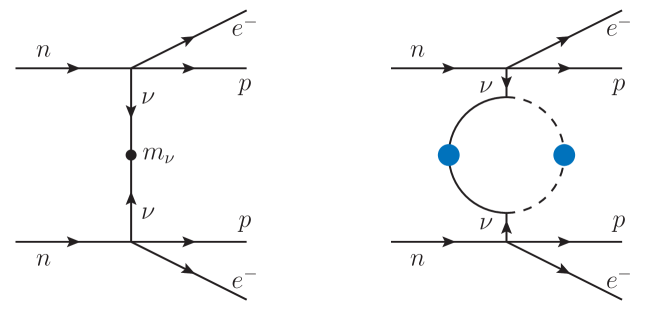
Figure 1: Left: Feynman diagram of the standard $0\nu\beta\beta$ decay process; Right: Feynman diagram of a loop-enhanced $0\nu\beta\beta$ decay process, where the blue blobs represent LNV, cf. Fig. 2.

In neutrino oscillation experiments the intermediate propagating neutrino mass states are essentially immediately (as soon as they travel a distance $x\sim 1/p$) on-shell, i.e. $p^{2}\approx 0$. In order to find a situation in which neutrinos are off-shell, or possess a large virtuality, we consider $0\nu\beta\beta$ decay. In this process, the exchanged Majorana neutrino (see Fig. 1) is off-shell. In fact, it has a momentum corresponding to the distance of the two neutrons participating in $0\nu\beta\beta$:

$$p^{2}\sim\frac{1}{r^{2}}.$$

The mean distance between neutrons for most heavy isotopes is:

$$\langle r\rangle\approx 1\ {\rm fm},$$

corresponding to an energy scale of 200 MeV. Therefore if neutrino masses are generated by a loop with $\Lambda$ not much higher than 200 MeV, then the $p^{2}/\Lambda^{2}$ term will make a considerable contribution to the $0\nu\beta\beta$ rate. In terms of diagrams, the loop that generates neutrino mass radiatively appears in the internal neutrino line of the process. The decay rate should thus be computed using the right diagram in Fig. 1 instead of the left standard diagram. The amplitude of the standard diagram is proportional to Majorana mass $m_{\nu}$. The loop effect can be easily included by replacing the Majorana mass $m_{\nu}$ with $\Sigma$. However, the loop effect on the total $0\nu\beta\beta$ decay rate is in general more complicated, since it involves an integral over the momentum $p$ when the full calculation of the decay rate is performed.

In the above discussion, we do not take the flavor structure into consideration. We need to generalize the neutrino self-energy $\Sigma$ and the mass $m_{\nu}$ to matrices with flavor indices ($\alpha$, $\beta$) added, such as $\Sigma\rightarrow\Sigma_{\alpha\beta}$, $m_{\nu}\rightarrow(m_{\nu})_{\alpha\beta}$. Since $\Lambda$ is defined in the $p$-expansion of $\Sigma$, it has the same flavor indices as $\Sigma$. In addition, the neutrino self-energy may receive several loop contributions in realistic models, such as $\Sigma=\Sigma_{1}+\Sigma_{2}+\Sigma_{3}+\cdots$. An example, discussed later in Sec. IV, is the scotogenic model in which three right-handed neutrinos are present, effectively generating neutrino mass by three 1-loop diagrams. Each contribution $\Sigma_{j}$ has a similar $p$-expansion as Eq. (4), with corresponding coefficients $m_{\nu j}$ and $\Lambda_{j}$. When summing these contributions together, one can still use Eq. (4) with the total neutrino mass matrix $m_{\nu}=m_{\nu 1}+m_{\nu 2}+m_{\nu 3}+\cdots$ and $\Lambda^{2}$ given by:

$$\frac{1}{\Lambda^{2}}=\sum_{j}\frac{1}{\Lambda_{j}^{2}}\frac{m_{\nu j}}{m_{\nu}}\,.$$ (5)

Note that Eq. (5) should be computed at the level of each matrix element. For instance, $\frac{1}{m_{\nu}}$ should be taken simply as $((m_{\nu})_{\alpha\beta})^{-1}$, rather than the inverse of the matrix $m_{\nu}$ which would be $(m^{-1}_{\nu})_{\alpha\beta}$.

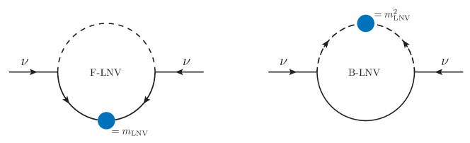
Figure 2: Lepton-number-violating neutrino self-energy diagrams at the 1-loop level. To connect two external neutrino lines, the loop can only consist of a bosonic line and a fermionic line. To generate Majorana neutrino masses, the loop must contain lepton number violation (indicated by the blue blobs). This can enter either in the fermionic part (left plot) or in the bosonic part (right) of the loop. Throughout this paper, we refer to the former as F-LNV and the latter as B-LNV.

Now let us discuss the generic topology of 1-loop diagrams that can generate Majorana neutrino masses. Since the loop must connect two external fermion legs ($\nu_{L}$ and $\overline{\nu_{L}^{c}}$), it must consist of a fermion line and a boson line, as illustrated by the diagrams in Fig. 2. This is the only possible topology for all 1-loop diagrams generating neutrino mass. The loops may have additional scalar boson lines attached (e.g., Fig. 4), which eventually end as vacuum expectation values (VEVs). Such lines can be removed in the context of computing the neutrino self-energy, as their effects will be absorbed into the masses of particles running in the loops. Next, generating Majorana neutrino masses requires sources of lepton number violation (LNV), which can appear either in the fermionic part or in the bosonic part of the loop, see Fig. 2. We refer to the two cases as Fermionic LNV (F-LNV) and Bosonic LNV (B-LNV), and discuss them separately in what follows.

II.1 F-LNV

The left diagram in Fig. 2 shows an F-LNV loop for radiative neutrino mass generation. The LNV insertion (the blue blob) is essentially a Majorana mass, though in complete models it may stand for more complex structures that eventually give rise to such an effective mass. Denoting the Majorana mass as $m_{\text{LNV}}$, the product of the two Yukawa vertices as $y^{2}$, and the fermion/boson running in the loop as $\psi$/$\phi$, respectively, we can compute this diagram directly. Here we present the result and delegate the detailed calculation to Appendix A.

The neutrino self-energy generated by the F-LNV loop is

$$\Sigma = \frac{y^{2}}{16\pi^{2}}m_{\text{LNV}}$$ (6)

$$\times\left[\frac{1}{\epsilon}+1-\frac{m_{\phi}^{2}\ln m_{\phi}^{2}-m_{\psi}^{2}\ln m_{\psi}^{2}}{m_{\phi}^{2}-m_{\psi}^{2}}+\frac{m_{\phi}^{4}-m_{\psi}^{4}-2m_{\psi}^{2}m_{\phi}^{2}\ln\frac{m_{\phi}^{2}}{m_{\psi}^{2}}}{2\left(m_{\phi}^{2}-m_{\psi}^{2}\right){}^{3}}p^{2}+{\cal O}(p^{4})\right],$$

where $p$ is the neutrino momentum and $\epsilon=(4-d)/2$ is the commonly-used notation in dimensional regularization. The masses of $\psi$ and $\phi$ are denoted as $m_{\psi}$ and $m_{\phi}$, respectively.

As can be expected, the result is proportional to $y^{2}$ and $m_{{\rm LNV}}$, with a typical loop-suppression factor $(16\pi^{2})^{-1}$. Putting $\frac{y^{2}}{16\pi^{2}}m_{\text{LNV}}$ aside, the remaining part, though a little complicated, can be simply summarized as some ratios of $m_{\psi}$, $m_{\phi}$ and $p^{2}$, independent of $m_{\text{LNV}}$. The UV divergence $\frac{1}{\epsilon}$ is expected in the F-LNV loop, but it will get cancelled in a complete renormalisable model —see, e.g., the scotogenic model discussed in Sec. IV. Note that from now on every time terms like $\ln m_{x}^{2}$ appear in the expressions, it is understood that they actually read $\ln m_{x}^{2}/\mu^{2}$, with $\mu^{2}$ is the renormalization scale. Again, in complete renormalisable theories there is no dependence on $\mu^{2}$. In the presence of such complete models, $\frac{1}{\epsilon}$ is usually replaced by a model-dependent ${\cal O}(1)$ quantity. When adopting a model-independent approach, it is usually safe to disregard the $\frac{1}{\epsilon}$ part and just keep in mind that the results may have ${\cal O}(1)$ uncertainties. See Refs. Bischer:2018zbd ; Xu:2019dxe for similar approaches.

Note that in some models where $\psi$ is simply a right-handed neutrino, $m_{\text{LNV}}$ and $m_{\psi}$ are identical. We prefer to have two different masses here for more general consideration and also for more manifest physical meaning of the expression. On the other hand, the two fermion propagators connected by $m_{{\rm LNV}}$ could be of different fermions with different masses, and each of the propagators (including the one of the boson) could be further split into two or more propagators. In this case, the result will have more complicated mass dependence — see Eqs. (36) and (37) for example. We refrain from introducing more mass parameters here since two masses are sufficient to illustrate the generic features of the F-LNV loop to be discussed below.

Let us discuss interesting limits of Eq. (6) which can help us to further understand the dependence of the F-LNV loop on the masses.

$\bullet$ Domination of $m_{\phi}$ ($m_{\psi}\ll m_{\phi}$):

When $m_{\psi}$ is much smaller than $m_{\phi}$, the result turns out to be dominated by the contribution of $m_{\phi}$. In the limit $m_{\psi}\rightarrow 0$, Eq. (6) reduces to

$$\Sigma=\frac{y^{2}}{16\pi^{2}}m_{\text{LNV}}\left[\frac{1}{\epsilon}+1-\ln m_{\phi}^{2}+\frac{p^{2}}{2m_{\phi}^{2}}+{\cal O}(p^{4})\right].$$ (7)

For small nonzero $m_{\psi}$, the next-to-leading order (NLO) correction to the terms in the square bracket in Eq. (7) is:

$$\frac{m_{\psi}^{2}}{m_{\phi}^{2}}\ln\frac{m_{\psi}^{2}}{m_{\phi}^{2}}+\frac{m_{\psi}^{2}}{2m_{\phi}^{4}}\left(3+2\frac{m_{\psi}^{2}}{m_{\phi}^{2}}\ln\frac{m_{\psi}^{2}}{m_{\phi}^{2}}\right)p^{2}\,.$$ (8)

$\bullet$ Domination of $m_{\psi}$ ($m_{\psi}\gg m_{\phi}$):

Similarly, when $m_{\phi}$ is much smaller than $m_{\psi}$, the result is not sensitive to $m_{\phi}$. Taking the limit $m_{\phi}\rightarrow 0$, Eq. (6) reduces to

$$\Sigma=\frac{y^{2}}{16\pi^{2}}m_{\text{LNV}}\left[\frac{1}{\epsilon}+1-\ln m_{\psi}^{2}+\frac{p^{2}}{2m_{\psi}^{2}}+{\cal O}(p^{4})\right].$$ (9)

The NLO correction of small nonzero $m_{\phi}$ to the terms in the square bracket in Eq. (9) is

$$\frac{m_{\phi}^{2}}{m_{\psi}^{2}}\ln\frac{m_{\phi}^{2}}{m_{\psi}^{2}}+\frac{m_{\phi}^{2}}{2m_{\psi}^{4}}\left(3+2\frac{m_{\phi}^{2}}{m_{\psi}^{2}}\ln\frac{m_{\phi}^{2}}{m_{\psi}^{2}}\right)p^{2}\,.$$ (10)

Note that Eqs. (9) and (10) can be obtained by interchanging $m_{\psi}\leftrightarrow m_{\phi}$ in Eqs. (7) and (8), since Eq. (6) is symmetric under $m_{\psi}\leftrightarrow m_{\phi}$.

$\bullet$ The $m_{\psi}=m_{\phi}$ case:

At first sight Eq. (6) seems to possess a singularity when $m_{\psi}$ approaches $m_{\phi}$. However, for $m_{\psi}=m_{\phi}=m$, Eq. (6) reduces to:

$$\Sigma=\frac{y^{2}}{16\pi^{2}}m_{\text{LNV}}\left(\frac{1}{\epsilon}-\ln m^{2}+\frac{p^{2}}{6m^{2}}+{\cal O}(p^{4})\right).$$ (11)

From the above discussions, we can summarize that F-LNV loops typically generate a result of the form given in Eq. (4), where the energy scale $\Lambda$ is mainly determined by the largest mass in the loop:

$$\Lambda\approx{\cal O}\left[\max(m_{\psi},\ m_{\phi})\right].$$ (12)

We will show in the next subsection that B-LNV loops generate similar result—for comparison, see Tab. 1.

Table 1: Neutrino masses ($m_{\nu}$) and self-energies ($\Sigma$) obtained from computing the 1-loop F-LNV and B-LNV diagrams in Fig. 2.

	$m_{\phi}$-dominated	$m_{\psi}$-dominated
F-LNV	$m_{\nu}=\frac{y^{2}}{16\pi^{2}}m_{{\rm LNV}}\times{\cal O}(1)$	$m_{\nu}=\frac{y^{2}}{16\pi^{2}}m_{{\rm LNV}}\times{\cal O}(1)$
	$\Sigma\approx m_{\nu}\left[1+\frac{p^{2}}{m_{\phi}^{2}}\times{\cal O}(1)\right]$	$\Sigma\approx m_{\nu}\left[1+\frac{p^{2}}{m_{\psi}^{2}}\times{\cal O}(1)\right]$
B-LNV	$m_{\nu}=\frac{y^{2}}{16\pi^{2}}m_{{\rm LNV}}^{2}\frac{m_{\psi}}{m_{\phi}^{2}}\times{\cal O}(1)$	$m_{\nu}=\frac{y^{2}}{16\pi^{2}}\frac{m_{{\rm LNV}}^{2}}{m_{\psi}}\times{\cal O}(1)$
	$\Sigma\approx m_{\nu}\left[1+\frac{p^{2}}{m_{\phi}^{2}}\times{\cal O}(1)\right]$	$\Sigma\approx m_{\nu}\left[1+\frac{p^{2}}{m_{\psi}^{2}}\times{\cal O}(1)\right]$

II.2 B-LNV

If neutrino masses are generated by a B-LNV loop shown in the right plot of Fig. 2, Majorana fermions are not required. Instead, the scalar boson in the loop has to carry lepton number and, typically via some VEV insertion, breaks it. The minimal UV-complete model that generates neutrino masses via a B-LNV loop, to our knowledge, is the Zee model Zee:1980ai . In the Zee model, the fermion running in the loop is a SM charged lepton, and the LNV part of the loop is achieved by a trilinear interaction of an $SU(2)_{L}$ singlet scalar scalar and two Higgs doublets. The latter obtain nonzero VEVs, which effectively give rise to the B-LNV structure discussed here—see Fig. 2 of Ref. Zee:1980ai .

Note that the blue blob in the right panel of Fig. 2 has dimension of $[{\rm mass}]{}^{2}$, which we shall denote as $m_{\text{LNV}}^{2}$. This is an important difference between the F-LNV and B-LNV loops. In Appendix A, we calculate the B-LNV loop. Using a similar notation as in the previous analysis on F-LNV, the calculation results in:

$$\Sigma = \frac{y^{2}}{16\pi^{2}}m_{\text{LNV}}^{2}m_{\psi}\frac{m_{\psi}^{2}-m_{\phi}^{2}+m_{\psi}^{2}\ln\frac{m_{\phi}^{2}}{m_{\psi}^{2}}}{\left(m_{\phi}^{2}-m_{\psi}^{2}\right){}^{2}}$$ (13)

$$\times\left[1-\frac{m_{\phi}^{4}+4m_{\psi}^{2}m_{\phi}^{2}-5m_{\psi}^{4}-2\left(m_{\psi}^{2}+2m_{\phi}^{2}\right)m_{\psi}^{2}\ln\frac{m_{\phi}^{2}}{m_{\psi}^{2}}}{2\left(m_{\phi}^{2}-m_{\psi}^{2}\right){}^{2}\left(m_{\psi}^{2}-m_{\phi}^{2}+m_{\psi}^{2}\ln\frac{m_{\phi}^{2}}{m_{\psi}^{2}}\right)}p^{2}+{\cal O}(p^{4})\right].$$

Since the B-LNV loop contains two scalar mediators and one fermion mediator, the loop integral is finite so there is no UV divergence in Eq. (13). Similar to the previous discussion on F-LNV, we can also derive some useful limits for B-LNV:

$\bullet$ Domination of $m_{\phi}$ ($m_{\psi}\ll m_{\phi}$):

When $m_{\psi}\ll m_{\phi}$, the denominators and numerators in Eq. (13) will be dominated by the highest powers of $m_{\phi}$, leading to:

$$\Sigma=-\frac{y^{2}}{16\pi^{2}}m_{\text{LNV}}^{2}m_{\psi}\left[\frac{1}{m_{\phi}^{2}}+\frac{p^{2}}{2m_{\phi}^{4}}+{\cal O}(p^{4})\right],$$ (14)

which implies that for large $m_{\phi}$, the neutrino self-energy and mass are suppressed by $\frac{1}{m_{\phi}^{2}}$.

$\bullet$ Domination of $m_{\psi}$ ($m_{\psi}\gg m_{\phi}$):

When $m_{\psi}\gg m_{\phi}$, the denominators and numerators in Eq. (13) will be dominated by the highest powers of $m_{\psi}$, leading to:

$$\Sigma=\frac{y^{2}}{16\pi^{2}}\frac{m_{\text{LNV}}^{2}}{m_{\psi}}\left[\ln\frac{m_{\phi}^{2}}{m_{\psi}^{2}}+1+\frac{2\ln\frac{m_{\phi}^{2}}{m_{\psi}^{2}}+5}{2m_{\psi}^{2}}p^{2}+{\cal O}(p^{4})\right],$$ (15)

which implies that for large $m_{\psi}$, the neutrino self-energy and mass are suppressed by $\frac{1}{m_{\psi}}$.

$\bullet$ The $m_{\psi}=m_{\phi}$ case:

After expanding Eq. (13) in terms of $m_{\psi}-m_{\phi}=\delta m$ and then taking the leading order, we get

$$\Sigma=-\frac{y^{2}}{16\pi^{2}}m_{\text{LNV}}^{2}\frac{1}{m}\left[\frac{1}{2}+\frac{1}{12m^{2}}p^{2}+{\cal O}(p^{4})\right],$$ (16)

where $m\equiv m_{\psi}=m_{\phi}$. This implies that if $m_{\psi}$ and $m_{\phi}$ both are large and of the same order $m$, then the neutrino self-energy and mass are suppressed by $\frac{1}{m}$.

Therefore, the neutrino self-energy generated by the B-LNV loop, in the three cases discussed above, can also be summarized by Eq. (4) where $\Lambda$ is, again, mainly determined by the largest mass in the loop—see Eq. (12). However, the neutrino mass $m_{\nu}$ in Eq. (4) in the B-LNV case is generically suppressed by the largest mass in the loop (see the summary in Tab. 1), unlike the F-LNV case, where $m_{\nu}$ is typically proportional to $\frac{y^{2}}{16\pi^{2}}$ and $m_{\text{LNV}}$ without further mass suppression. This is because the B-LNV and F-LNV loops are generically proportional to $m_{\text{LNV}}^{2}$ and $m_{\text{LNV}}$ respectively. Simply by dimensional arguments, the former needs to be attached with some quantity that has dimension of $[{\rm mass}]^{-1}$, which turns out to be $m_{\psi}/m_{\phi}^{2}$ in the $m_{\phi}$-dominated case, and $1/m_{\psi}$ in the $m_{\psi}$-dominated case.

III Phenomenology

In the standard scenario, the amplitude of $0\nu\beta\beta$ is proportional to $ee$-element of the neutrino mass matrix, given by

$$\langle m_{\beta\beta}\rangle=\left|m_{1}c_{12}^{2}c_{13}^{2}+e^{2i\alpha}m_{2}s_{12}^{2}c_{13}^{2}+e^{2i\beta}m_{3}s_{13}^{2}\right|,$$ (17)

where $s_{12}^{2}=1-c_{12}^{2}\approx 0.297$; $s_{13}^{2}=1-c_{13}^{2}\approx 2.14\times 10^{-2}$; $\alpha$ and $\beta$ are two unknown Majorana phases; the neutrino masses $m_{1}$, $m_{2}$ and $m_{3}$ can be determined from the two observed mass-squared differences, given the value of the lightest neutrino mass and the mass ordering (normal or inverted).

As explained above, if there is a single 1-loop diagram generating neutrino mass, and the involved particles are not much heavier than the neutrino’s virtuality of ${\cal O}(100)$ MeV, we can replace the effective mass with (see the right diagram in Fig. 1)

$$\langle m_{\beta\beta}\rangle\to\langle m_{\beta\beta}\rangle\left(1+\frac{p^{2}}{\Lambda^{2}}\right).$$ (18)

This would enhance or supress the amplitude by a common ${\cal O}(1)$ factor, depending on the sign of the correction. Recall that the decay rate, as previously discussed, involves an integral over the neutrino momentum $p$, implying in an explicit model an additional relative coefficient in front of $\frac{p^{2}}{\Lambda^{2}}$ that comes from this issue. We can ignore this complication, or alternatively assume that this factor can be hidden by redefining $\Lambda$. In Fig. 3 we show an example for the redefined effective mass that is a factor of 2 smaller or larger than the standard case. Interesting things could happen. For instance, within the inverted ordering, one could interpret the measurement as an effective mass value lower than the usual minimal value in this case. One would assume now that another mechanism, probably of TeV-scale, generates the decay and that neutrinos are mainly Dirac or that the alternative TeV-scale mechanism interferes negatively with the standard neutrino diagram. However, it is more or less the usual diagram that mediates the decay, simple the self-energy term plays an important role. A similar example is when, for quasi-degenerate neutrinos, the measurement would be interpreted as an effective mass value above the maximal allowed value for this case.

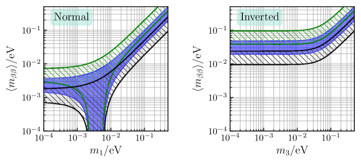
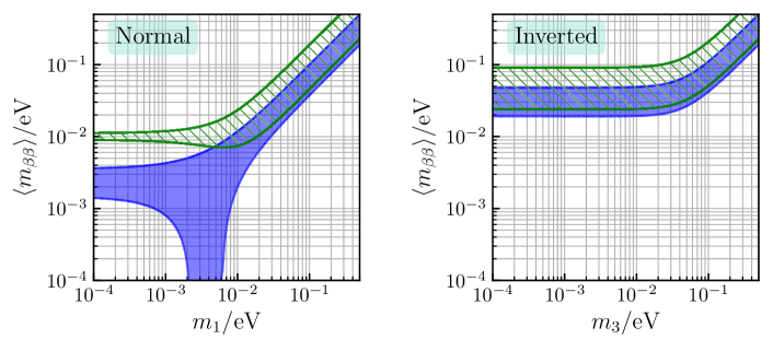
Figure 3: Loop-modified $0\nu\beta\beta$ decay. The blue regions are the standard predictions of $\langle m_{\beta\beta}\rangle$ constructed from current best-fit values of oscillation parameters and arbitrary Majorana phases. The upper plots assume a common suppression (black hatched) or enhancement (green hatched) of the effective mass by a factor of 2. The lower plots assume that $\Lambda_{2}^{2}=\langle p^{2}\rangle/3$ and negligible contributions from $\Lambda_{1}$ and $\Lambda_{3}$, see Eq. (19). The left and right plots are for the normal and inverted mass ordering, respectively.

Within a loop mechanism for neutrino mass there can be several contributions to the neutrino mass matrix, see Eq. (5). This can be readily included into the $0\nu\beta\beta$ amplitude by the following replacement:

$$m_{i}\rightarrow m_{i}\left(1+\frac{p^{2}}{\Lambda_{i}^{2}}\right),\ (i=1,\ 2,\ 3),$$ (19)

where $\Lambda_{1}$, $\Lambda_{2}$, and $\Lambda_{3}$ in principle can be different. When $\Lambda_{1}=\Lambda_{2}=\Lambda_{3}\equiv\Lambda$, we have the case discussed above, i.e. an overall enhancement or suppression of the amplitude. When $\Lambda_{1}$, $\Lambda_{2}$, and $\Lambda_{3}$ are different, however, there can be more interesting phenomenology. For example, it has been well known that in the normal mass ordering, vanishing $\langle m_{\beta\beta}\rangle$ is possible due to cancellation among the three terms in Eq. (17). If $m_{1}$, $m_{2}$ and $m_{3}$ are enhanced or suppressed differently, then such cancellation may be less complete or even disappear. As an illustrative example, in Fig. 3 we show how $\langle m_{\beta\beta}\rangle$ can be changed if $\Lambda_{2}^{2}=\langle p^{2}\rangle/3$, while $\Lambda_{1}^{2}$ and $\Lambda_{2}^{2}$ are assumed to be much larger than $\langle p^{2}\rangle$ so that their effects are negligible. We can see for both the normal and inverted mass ordering that $\langle m_{\beta\beta}\rangle$ is enhanced from the blue standard regions to the new green regions. The most noteworthy change is that $\langle m_{\beta\beta}\rangle$ in the normal mass ordering cannot vanish anymore.

IV The scotogenic model as an example

Now we shall apply our so far model-independent study to a specific example, by choosing the scotogenic model Ma:2006km . By adding a new Higgs doublet and singlet fermions to the SM, and introducing an unbroken $Z_{2}$ symmetry, the scotogenic model successfully accommodates a dark matter candidate and radiatively generates neutrino masses in a very economic way.

Denoting the new Higgs doublet and the singlet fermions as $\eta=(\eta^{+},\ \eta^{0})^{T}$ and $N_{j}$, the model can be formulated as follows:

$${\cal L} = {\cal L}_{{\rm{\rm SM}}}-y_{\alpha j}\overline{L_{\alpha}}\tilde{\eta}N_{j}-\frac{1}{2}M_{j}\overline{N_{j}^{c}}N_{j}+|D\eta|^{2}-m_{\eta}^{2}\eta^{\dagger}\eta+\left({\rm terms\ of\ }\mbox{$\eta$}^{4}\ {\rm and}\ \eta^{2}H^{2}\right).$$ (20)

Here $y_{\alpha j}$ is the Yukawa coupling matrix with a flavor index $\alpha=e,\ \mu,\ \tau$ and a mass-eigenstate index $j=1,\ 2,\ 3$; $L$ is a left-handed lepton doublet, and $\tilde{\eta}=(\eta^{0},\ -\eta^{+})^{\dagger}$. Without loss of generality, we have diagonalized the Majorana mass matrix of the $N_{j}$ in Eq. (20) to its mass eigenvalues $M_{j}$. The SM Higgs doublet $H$ does not couple to neutrinos directly due to the $Z_{2}$ symmetry: $N_{j}\rightarrow-N_{j}$, $\eta\rightarrow-\eta$. Therefore, the usual Dirac mass in the Type I seesaw is forbidden and the left-handed neutrinos are massless at tree level.

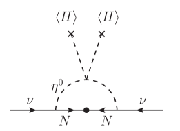
Figure 4: Feynman diagram for neutrino mass generation in the scotogenic model.

The model generates neutrino masses at the 1-loop level via the diagram presented in Fig. 4. As shown in this diagram, this is in our language an F-LNV loop. It consists of $\eta^{0}$ (the neutral component of $\eta$) and $N_{j}$ mediators, hence there are three different diagrams, corresponding to $N_{1,2,3}$. Their Majorana masses serve as the source of LNV. After electroweak symmetry breaking, we replace the SM Higgs in this diagram by its VEV ($\eta$ does not obtain a VEV), which eventually contributes to the masses of the scalar bosons running in the loop. Including the contribution of the SM Higgs VEV, the real and imaginary parts of $\eta^{0}$ become mass eigenstates with different masses, denoted as $m_{R}$ and $m_{I}$, respectively. According to Ref. Ma:2006km , the neutrino masses generated in this model are

$$\left(m_{\nu}\right)_{\alpha\beta}=\frac{y_{\alpha j}y_{\beta j}}{16\pi^{2}}M_{j}\left[\frac{m_{R}^{2}}{m_{R}^{2}-M_{j}^{2}}\ln\frac{m_{R}^{2}}{M_{j}^{2}}-\frac{m_{I}^{2}}{m_{I}^{2}-M_{j}^{2}}\ln\frac{m_{I}^{2}}{M_{j}^{2}}\right].$$ (21)

This result can also be quite straightforwardly obtained using our model-independent calculation in Sec. II. From Eq. (6), we can immediately write down the result in the case of ${\rm Re}(\eta^{0})$ running in the loop, simply by replacing $y^{2}\rightarrow y_{\alpha j}y_{\beta j}$, $m_{{\rm LNV}}\rightarrow M_{j}$, $m_{\psi}\rightarrow M_{j}$, and $m_{\phi}\rightarrow m_{R}$. The contribution of the imaginary part ${\rm Im}(\eta^{0})$ is similar but differs by a minus sign because the Yukawa coupling of ${\rm Im}(\eta^{0})$ is attached with an additional $i$: $y^{2}\rightarrow(iy_{\alpha j})(iy_{\beta j})=-y_{\alpha j}y_{\beta j}$. Due to this minus sign, the terms $\frac{1}{\epsilon}+1$ in Eq. (6) from diagrams containing the real and imaginary parts of $\eta^{0}$ cancel each other. The neutrino self-energy after this cancellation can be written as follows:

$$\Sigma_{\alpha\beta}=\left(m_{\nu}\right)_{\alpha\beta}\left[1+\frac{p^{2}}{\Lambda^{2}}+{\cal O}(p^{4})\right],$$ (22)

where

$$\Lambda^{2}=2\frac{\frac{m_{R}^{2}}{m_{R}^{2}-M_{j}^{2}}\ln\frac{m_{R}^{2}}{M_{j}^{2}}-\frac{m_{I}^{2}}{m_{I}^{2}-M_{j}^{2}}\ln\frac{m_{I}^{2}}{M_{j}^{2}}}{\frac{M_{j}^{4}-m_{R}^{4}+2m_{R}^{2}M_{j}^{2}\ln\frac{m_{R}^{2}}{M_{j}^{2}}}{\left(m_{R}^{2}-M_{j}^{2}\right)^{3}}-\frac{M_{j}^{4}-m_{I}^{4}+2m_{I}^{2}M_{j}^{2}\ln\frac{m_{I}^{2}}{M_{j}^{2}}}{\left(m_{I}^{2}-M_{j}^{2}\right)^{3}}}\,.$$ (23)

Eq. (23) applies only to a single $M_{j}$ contribution, while to include multiple contributions one needs to use Eq. (5).

The expression (23) is rather complicated. In what follows, we would like to focus on one hierarchical scenario ($M_{j}\ll m_{R}\ll m_{I}$) to discuss the phenomenology. First, for $m_{\psi}\ll m_{R,I}$, the expansion in $M_{j}$ simplifies Eq. (23) to

$$\Lambda^{2}=\frac{2m_{I}^{2}m_{R}^{2}}{m_{I}^{2}-m_{R}^{2}}\ln\frac{m_{I}^{2}}{m_{R}^{2}}+{\cal O}(M_{j}^{2}).$$ (24)

Then, assuming $m_{R}\ll m_{I}$, Eq. (24) further simplifies to

$$\Lambda^{2}\approx 2m_{R}^{2}\ln\frac{m_{I}^{2}}{m_{R}^{2}},\ {\rm for}\ M_{j}\ll m_{R}\ll m_{I},$$ (25)

which implies that the energy scale of the loop in this scenario is mainly determined by $m_{R}$, as long as the hierarchy $M_{j}\ll m_{R}\ll m_{I}$ holds.

Now we need to know how small $m_{R}$ and $M_{j}$ can be in this model. First, let us inspect the singlet fermion masses. If $M_{j}$ is too light, it would not generate the correct values of neutrino masses, which should be around $0.05$ to $0.1$ eV. So without any particular cancellation, Eq. (21) implies that $M_{j}$ needs to be above $16\pi^{2}\times m_{\nu}={\cal O}(10)$ eV, assuming that the Yukawa couplings cannot be much larger than ${\cal O}(1)$. For smaller Yukawa couplings, $M_{j}$ correspondingly needs to be higher. On the other hand, if the singlet fermions are lighter than a few MeV with sizable coupling, they contribute to the effective number of neutrinos in the early universe, excluded by BBN and CMB observations. Therefore, to evade such bounds, we assume that $M_{j}\gtrsim 10$ MeV. With this assumption, we get $y\sim 4\pi\sqrt{m_{\nu}/M_{j}}\lesssim 10^{-3}$, which is below meson decay bounds Barger:1981vd ; Lessa:2007up ; Pasquini:2015fjv on neutrino-scalar couplings. Note that the neutral $\eta^{0}$ does not couple to charged leptons or quarks and can easily evade observational constraints. The scalar masses $m_{R}$ and $m_{I}$ cannot be both very light otherwise the SM $Z$ boson would decay to ${\rm Re}(\eta^{0})$ and ${\rm Im}(\eta^{0})$. Therefore we only consider the case that $m_{I}$ is well above the $Z$ mass while $m_{R}$ is much lighter. Other collider constraints on $\eta$ include charged Higgs searches at LEP and LEP II, electroweak precision test, and Higgs invisible decay—see Refs. Lundstrom:2008ai ; Dolle:2009fn for a detailed discussion. Charged Higgs searches have set a lower bound on the mass of $\eta^{\pm}$ in the form of $m_{\pm}\gtrsim 70$–$90$ GeV Pierce:2007ut . This combined with electroweak precision tests puts a similar bound on $m_{I}$ because the $T$-parameter requires that $(m_{\pm}-m_{I})(m_{\pm}-m_{R})$ must be small Lundstrom:2008ai . To obey both constraints, we set $m_{\pm}=m_{I}\gtrsim 100$ GeV. Higgs invisible decay could provide potentially important constraints since the SM Higgs could decay to two ${\rm Re}(\eta^{0})$ particles if their mass $m_{R}$ is light. However, the current Higgs data from the LHC still allows for about 10% to 20% invisible decay width Aaboud:2018sfi ; Sirunyan:2018owy . On the other hand, the invisible decay width in this model can be suppressed by tuning the quartic couplings in the scalar potential while still keeping the above scenario viable Barbieri:2006dq . Such tuning is a general feature when one wants to be in the interesting situation in which the full 1PI diagram of the radiative neutrino mass mechanism is experimentally accessible for $0\nu\beta\beta$.

Nevertheless, we conclude that in the scotogenic model, at least the parameter space with $m_{R}\gtrsim M_{j}\gtrsim 10$ MeV and $m_{\pm}=m_{I}\gtrsim 100$ GeV is allowed by various constraints. Within this parameter space, $\Lambda$ in Eq. (23) can reach any value above the following bound:

$$\Lambda\gtrsim 111\ {\rm MeV}.$$ (26)

Taking $m_{R}=30$ MeV, $M_{j}=10$ MeV and $m_{\pm}=m_{I}=200$ GeV for example (corresponding to $m_{\nu}\sim y^{2}$ MeV, which reproduces the typical neutrino mass scale for permille-level Yukawa couplings), Eq. (25) gives $178$ MeV while the full expression (23) gives $\Lambda\approx 209\ {\rm MeV}$. This implies that $\Lambda$ in the scotogenic model can indeed be of the order of ${\cal O}(100)$ MeV.

V Conclusion

Radiative neutrino mass mechansims generate neutrino mass via a self-energy diagram in which one sets the external momentum to zero. The difference between the mass and the self-energy is usually not accessible in neutrino oscillation experiments as long as the neutrinos are on-shell. An interesting exception is neutrinoless double beta decay for which the neutrino virtuality is of order 100 MeV. Accepting the possibility that the particles in the neutrino-mass loop have masses around this scale, implies that higher order or even the full self-energy diagram have an effect in the decay. We performed a general study on the form of the diagram, and gave possible phenomenological consequences of a modified double beta decay amplitude. The scotogenic model was used as an explicit example to demonstrate that low-mass particles are possible in realistic models.

One can of course generalise the analysis to 2-, 3-, $n$-loop mechanisms for neutrino mass. We should note that there are radiative mechansims for Dirac neutrinos, which do not offer the option to see effects of the self-energy diagram if they do not contain LNV.

Appendix A Loop calculation of the F-LNV and B-LNV diagrams

Since the calculation involves charge conjugations of Dirac spinors, we would like to review a few identities which will be used. First, the notation $\psi^{c}$ of the general Dirac spinor $\psi$ is defined as $\psi^{c}=-i\gamma^{2}\psi^{*}$, so we have

$$\psi^{c}=\gamma^{c}\psi^{*},\ \overline{\psi^{c}}=\left(\gamma^{c}\psi^{*}\right)^{\dagger}\gamma^{0}=\left(\gamma^{0}\gamma^{c}\psi\right)^{T}\,,$$ (27)

where we have introduced $\gamma^{c}\equiv-i\gamma^{2}$ for simplicity. We are working with the chiral representations of Dirac matrices so that

$$\gamma^{0}=\left(\gamma^{0}\right)^{T}=\left(\gamma^{0}\right)^{\dagger},\ \gamma^{c}=\left(\gamma^{c}\right)^{T}=\left(\gamma^{c}\right)^{\dagger},\ \left(\gamma^{0}\gamma^{c}\right)^{T}=-\gamma^{0}\gamma^{c}\,.$$ (28)

In this convention, the transpose of $\gamma^{\mu}$ can be written as

$$\left(\gamma^{\mu}\right)^{T}=\gamma^{0}\gamma^{c}\gamma^{\mu}\gamma^{0}\gamma^{c}\,,$$ (29)

which can be useful when computing the transpose of a Dirac propagator. With the above notations and identities, we can convert the following Dirac propagators to each other:

$$\Delta_{\psi}\equiv\langle\psi\overline{\psi}\rangle\,,\ \Delta_{\psi}^{c}\equiv\langle\overline{\psi^{c}}\,\overline{\psi}\rangle\,.$$

Compared to the well-known propagator $\Delta_{\psi}$, the second propagator $\Delta_{\psi}^{c}$ is given less often, so here we derive it briefly. Let us denote the Dirac indices (using $e$, $f$, $g$, $\cdots$) explicitly, then we have

$$\left[\Delta_{\psi}^{c}\right]_{ef}\equiv\langle\overline{\psi_{e}^{c}}\,\overline{\psi_{f}}\rangle=\langle\left(\gamma^{0}\gamma^{c}\psi\right)_{e}\overline{\psi_{f}}\rangle=\sum_{g}\langle\left(\gamma^{0}\gamma^{c}\right)_{eg}\psi_{g}\overline{\psi_{f}}\rangle=\sum_{g}\left(\gamma^{0}\gamma^{c}\right)_{eg}\left[\Delta_{\psi}\right]_{gf}=\gamma^{0}\gamma^{c}\Delta_{\psi}\,.$$ (30)

Denoting the mass and momentum of $\psi$ as $m_{\psi}$ and $q$ respectively, the explicit forms of $\Delta_{\psi}$, $\Delta_{\psi}^{c}$ and their transpose are

$$\Delta_{\psi}=\frac{i(\not{q}+m_{\psi})}{q^{2}-m_{\psi}^{2}}\,,\ \Delta_{\psi}^{T}=\frac{i(\gamma^{0}\gamma^{c}\not{q}\gamma^{0}\gamma^{c}+m_{\psi})}{q^{2}-m_{\psi}^{2}}\,,$$ (31)

$$\Delta_{\psi}^{c}=\gamma^{0}\gamma^{c}\frac{i(\not{q}+m_{\psi})}{q^{2}-m_{\psi}^{2}}\,,\ \left(\Delta_{\psi}^{c}\right)^{T}=\frac{i(\gamma^{0}\gamma^{c}\not{q}-m_{\psi})}{q^{2}-m_{\psi}^{2}}\,.$$ (32)

With these identities, let us compute the F-LNV and B-LNV loops.

$\bullet$ F-LNV:

For generality, we consider that the two fermion propagators are of two different fermions, denoted as $\psi$ and $\psi^{\prime}$. The relevant part of the Lagrangian is formulated as

$${\cal L}\supset y\phi\overline{\psi}\nu_{L}+y^{\prime}\phi\overline{\psi^{\prime}}\nu_{L}+m_{{\rm LNV}}\overline{\psi^{\prime c}}\psi\,.$$ (33)

Integrating out the $\phi$, $\psi$ and $\psi^{\prime}$ fields in Eq. (33) will lead to an effective operator of two neutrinos

$$\overline{\nu_{L}^{c}}\Sigma\nu_{L}=-\left(\gamma^{0}\gamma^{c}\Sigma\right){}_{fg}\left(\nu_{L}\right)_{f}\left(\nu_{L}\right)_{g}\,,$$ (34)

which can be computed using the F-LNV Feynman diagram in Fig. 2 and Eqs. (31) and (32):

$$-i\overline{\nu_{L}^{c}}\Sigma\nu_{L} =- yy^{\prime}\int\frac{dq^{4}}{(2\pi)^{4}}\overline{\nu_{L}^{c}}P_{L}\frac{i(\not{q}+m_{\psi})}{q^{2}-m_{\psi}^{2}}\left(-im_{{\rm LNV}}\right)\frac{i(\not{q}-m_{\psi^{\prime}})}{q^{2}-m_{\psi^{\prime}}^{2}}\frac{i}{(q-p)^{2}-m_{\phi}^{2}}P_{L}\nu_{L}$$ (35)

$$= \frac{yy^{\prime}}{16\pi^{2}}m_{{\rm LNV}}\left[I^{(0)}+I^{(2)}p^{2}+{\cal O}(p^{4})\right]\overline{\nu_{L}^{c}}\nu_{L}\,,$$

where we have used Package-X Patel:2015tea to evaluate the loop integral and expanded the result in terms of $p^{2}$ with $I^{(0)}$ and $I^{(2)}$ given by:

$$I^{(0)} = \frac{1}{\epsilon}+1-\ln m_{\psi}^{2}+\frac{m_{\phi}^{2}m_{\psi}+m_{\phi}^{2}m_{\psi^{\prime}}-m_{\psi}^{2}m_{\psi^{\prime}}}{\left(m_{\psi}^{2}-m_{\phi}^{2}\right)\left(m_{\psi}+m_{\psi^{\prime}}\right)}\ln\frac{m_{\phi}^{2}}{m_{\psi}^{2}}$$ (36)

$$+\frac{m_{\psi^{\prime}}^{3}}{\left(m_{\psi^{\prime}}^{2}-m_{\phi}^{2}\right)\left(m_{\psi}+m_{\psi^{\prime}}\right)}\ln\frac{m_{\phi}^{2}}{m_{\psi^{\prime}}^{2}}\,,$$

$$I^{(2)} = \frac{\left(m_{\phi}^{2}+m_{\psi}m_{\psi^{\prime}}\right)\left(m_{\phi}^{4}+m_{\phi}^{2}m_{\psi}^{2}+m_{\phi}^{2}m_{\psi^{\prime}}^{2}+m_{\psi}^{2}m_{\psi^{\prime}}^{2}-4m_{\phi}^{2}m_{\psi}m_{\psi^{\prime}}\right)}{2\left(m_{\phi}^{2}-m_{\psi}^{2}\right)^{2}\left(m_{\phi}^{2}-m_{\psi^{\prime}}^{2}\right)^{2}}+$$ (37)

$$+\frac{m_{\phi}^{2}}{m_{\psi}+m_{\psi^{\prime}}}\left(\frac{m_{\psi}^{3}}{\left(m_{\psi}^{2}-m_{\phi}^{2}\right)^{3}}\ln\frac{m_{\phi}^{2}}{m_{\psi}^{2}}+\frac{m_{\psi^{\prime}}^{3}}{\left(m_{\psi^{\prime}}^{2}-m_{\phi}^{2}\right)^{3}}\ln\frac{m_{\phi}^{2}}{m_{\psi^{\prime}}^{2}}\right).$$

Taking the $m_{\psi^{\prime}}\rightarrow m_{\psi}$ limit, one can straightforwardly obtain the result in Eq. (6).

$\bullet$ B-LNV:

Similar to the F-LNV case, we also consider that the two scalar propagators are of two different scalars, denoted as $\phi$ and $\phi^{\prime}$. The relevant part of the Lagrangian is formulated as

$${\cal L}\supset y\phi\overline{\psi^{c}}\nu_{L}+y^{\prime}\phi^{\prime}\thinspace\overline{\psi}\nu_{L}+m_{{\rm LNV}}^{2}\phi^{\prime*}\phi\,.$$ (38)

Integrating out the $\psi$, $\phi$ and $\phi^{\prime}$ gives

$$-i\overline{\nu_{L}^{c}}\Sigma\nu_{L} =- y^{2}\int\frac{dq^{4}}{(2\pi)^{4}}\overline{\nu_{L}^{c}}\frac{i(\not{q}-m_{\psi})}{q^{2}-m_{\psi}^{2}}\frac{i}{(q-p)^{2}-m_{\phi}^{2}}\left(-im_{{\rm LNV}}^{2}\right)\frac{i}{(q-p)^{2}-m_{\phi^{\prime}}^{2}}\nu_{L}$$ (39)

$$= -\frac{y^{2}}{16\pi^{2}}m_{{\rm LNV}}^{2}m_{\psi}\left[I^{(0)}+I^{(2)}p^{2}+{\cal O}(p^{4})\right]\overline{\nu_{L}^{c}}\nu_{L}\,,$$

where the result has been expanded in terms of $p^{2}$ with $I^{(0)}$ and $I^{(2)}$ given by:

$$I^{(0)} = \frac{1}{m_{\phi}^{2}-m_{\phi^{\prime}}^{2}}\left(\frac{m_{\phi^{\prime}}^{2}}{m_{\phi^{\prime}}^{2}-m_{\psi}^{2}}\ln\frac{m_{\phi^{\prime}}^{2}}{m_{\psi}^{2}}-\frac{m_{\phi}^{2}}{m_{\phi}^{2}-m_{\psi}^{2}}\ln\frac{m_{\phi}^{2}}{m_{\psi}^{2}}\right),$$ (40)

$$I^{(2)} = \frac{m_{\psi}^{2}}{m_{\phi}^{2}-m_{\phi^{\prime}}^{2}}\left(\frac{m_{\phi^{\prime}}^{2}}{\left(m_{\phi^{\prime}}^{2}-m_{\psi}^{2}\right)^{3}}\ln\frac{m_{\phi^{\prime}}^{2}}{m_{\psi}^{2}}-\frac{m_{\phi}^{2}}{\left(m_{\phi}^{2}-m_{\psi}^{2}\right)^{3}}\ln\frac{m_{\phi}^{2}}{m_{\psi}^{2}}\right)$$ (41)

$$-\frac{\left(m_{\phi^{\prime}}^{2}+m_{\phi}^{2}\right)m_{\psi}^{2}-3m_{\psi}^{4}+m_{\phi}^{2}m_{\phi^{\prime}}^{2}}{2\left(m_{\phi}^{2}-m_{\psi}^{2}\right)^{2}\left(m_{\phi^{\prime}}^{2}-m_{\psi}^{2}\right)^{2}}\,.$$

Taking the $m_{\phi^{\prime}}\rightarrow m_{\phi}$ limit, one can straightforwardly obtain the result in Eq. (13).

References

• (1) M. J. Dolinski, A. W. P. Poon, and W. Rodejohann, Neutrinoless Double-Beta Decay: Status and Prospects, Submitted to: Ann. Rev. Nucl. Part. Phys. (2019) [1902.04097].
• (2) W. Rodejohann, Neutrino-less Double Beta Decay and Particle Physics, Int. J. Mod. Phys. E20 (2011) 1833–1930, [1106.1334].
• (3) F. F. Deppisch, M. Hirsch, and H. Pas, Neutrinoless Double Beta Decay and Physics Beyond the Standard Model, J. Phys. G39 (2012) 124007, [1208.0727].
• (4) L. Graf, F. F. Deppisch, F. Iachello, and J. Kotila, Short-Range Neutrinoless Double Beta Decay Mechanisms, Phys. Rev. D98 (2018), no. 9 095023, [1806.06058].
• (5) K. S. Babu and C. N. Leung, Classification of effective neutrino mass operators, Nucl. Phys. B619 (2001) 667–689, [hep-ph/0106054].
• (6) E. Ma, Neutrino Mass: Mechanisms and Models, 0905.0221.
• (7) F. Bonnet, M. Hirsch, T. Ota, and W. Winter, Systematic study of the d=5 Weinberg operator at one-loop order, JHEP 07 (2012) 153, [1204.5862].
• (8) D. Aristizabal Sierra, A. Degee, L. Dorame, and M. Hirsch, Systematic classification of two-loop realizations of the Weinberg operator, JHEP 03 (2015) 040, [1411.7038].
• (9) C. Klein, M. Lindner, and S. Ohmer, Minimal Radiative Neutrino Masses, JHEP 03 (2019) 018, [1901.03225].
• (10) Y. Cai, J. Herrero-Garcia, M. A. Schmidt, A. Vicente, and R. R. Volkas, From the trees to the forest: a review of radiative neutrino mass models, Front.in Phys. 5 (2017) 63, [1706.08524].
• (11) F. Simkovic, A. Smetana, and P. Vogel, $0\nu\beta\beta$ nuclear matrix elements, neutrino potentials and $\mathrm{SU}(4)$ symmetry, Phys. Rev. C98 (2018), no. 6 064325, [1808.05016].
• (12) N. Shimizu, J. Menendez, and K. Yako, Double Gamow-Teller Transitions and its Relation to Neutrinoless $\beta\beta$ Decay, Phys. Rev. Lett. 120 (2018), no. 14 142502, [1709.01088].
• (13) I. Bischer, W. Rodejohann, and X.-J. Xu, Loop-induced Neutrino Non-Standard Interactions, JHEP 10 (2018) 096, [1807.08102].
• (14) X.-J. Xu, Tensor and scalar interactions of neutrinos may lead to observable neutrino magnetic moments, Phys. Rev. D99 (2019), no. 7 075003, [1901.00482].
• (15) A. Zee, A Theory of Lepton Number Violation, Neutrino Majorana Mass, and Oscillation, Phys. Lett. 93B (1980) 389. [Erratum: Phys. Lett.95B,461(1980)].
• (16) E. Ma, Verifiable radiative seesaw mechanism of neutrino mass and dark matter, Phys. Rev. D73 (2006) 077301, [hep-ph/0601225].
• (17) V. D. Barger, W.-Y. Keung, and S. Pakvasa, Majoron Emission by Neutrinos, Phys. Rev. D25 (1982) 907.
• (18) A. P. Lessa and O. L. G. Peres, Revising limits on neutrino-Majoron couplings, Phys. Rev. D75 (2007) 094001, [hep-ph/0701068].
• (19) P. S. Pasquini and O. L. G. Peres, Bounds on Neutrino-Scalar Yukawa Coupling, Phys. Rev. D93 (2016), no. 5 053007, [1511.01811]. [Erratum: Phys. Rev.D93,no.7,079902(2016)].
• (20) E. Lundstrom, M. Gustafsson, and J. Edsjo, The Inert Doublet Model and LEP II Limits, Phys. Rev. D79 (2009) 035013, [0810.3924].
• (21) E. M. Dolle and S. Su, The Inert Dark Matter, Phys. Rev. D80 (2009) 055012, [0906.1609].
• (22) A. Pierce and J. Thaler, Natural Dark Matter from an Unnatural Higgs Boson and New Colored Particles at the TeV Scale, JHEP 08 (2007) 026, [hep-ph/0703056].
• (23) ATLAS Collaboration, M. Aaboud et al., Search for invisible Higgs boson decays in vector boson fusion at $\sqrt{s}=13$ TeV with the ATLAS detector, Phys. Lett. B793 (2019) 499–519, [1809.06682].
• (24) CMS Collaboration, A. M. Sirunyan et al., Search for invisible decays of a Higgs boson produced through vector boson fusion in proton-proton collisions at $\sqrt{s}=$ 13 TeV, Phys. Lett. B793 (2019) 520–551, [1809.05937].
• (25) R. Barbieri, L. J. Hall, and V. S. Rychkov, Improved naturalness with a heavy Higgs: An Alternative road to LHC physics, Phys. Rev. D74 (2006) 015007, [hep-ph/0603188].
• (26) H. H. Patel, Package-X: A Mathematica package for the analytic calculation of one-loop integrals, Comput. Phys. Commun. 197 (2015) 276–290, [1503.01469].