First results from the WISPDMX radio frequency cavity searches for hidden photon dark matter

Abstract

The origin of non-baryonic dark matter remains elusive despite ongoing sensitive searches for heavy, thermally produced dark matter particles. Recently, it has been shown that non-thermally produced vector bosons (sometimes called hidden photons) related to a broken U(1) gauge symmetry are among the possible WISP (weakly interacting slim particles) dark matter candidates. The WISP Dark Matter eXperiment (WISPDMX) is the first direct hidden photon dark matter search experiment probing the particle masses within the $0.8\text{\,}\mathrm{\SIUnitSymbolMicro}\eV 2.07\text{\,}\mathrm{\SIUnitSymbolMicro}\eV$ range with four resonant modes of a tunable radio frequency cavity and down to $0.4\text{\,}\mathrm{n}\eV$ outside of resonance. In this paper, we present the results from the first science run of WISPDMX comprising $22\,000$ broadband spectra with a $500\text{\,}\mathrm{M}\Hz$ bandwidth and a $50\text{\,}\Hz$ spectral resolution, obtained during 10-second integrations made at each individual tuning step of the measurements. No plausible dark matter candidate signal is found, both in the individual spectra reaching minimum detectable power of $8\text{\times}{10}^{-19}\text{\,}\mathrm{W}$ and in the averaged spectrum of all the measurements with the minimum detectable power of $5\text{\times}{10}^{-22}\text{\,}\mathrm{W}$) attained for a total of $61\text{\,}\mathrm{h}$ of data taking. Using these spectra, we derive upper limits on the coupling constant of the hidden photon at the levels of ${10}^{-13}$ for the resonant frequency ranges and ${10}^{-12}$ for broadband mass range $0.2\text{\,}\mathrm{\SIUnitSymbolMicro}\eV 2.07\text{\,}\mathrm{\SIUnitSymbolMicro}\eV$, and steadily increasing at masses below $0.2\text{\,}\mathrm{\SIUnitSymbolMicro}\eV$.

1 Introduction

The standard model of particle physics (SM) has so far withstood all experimental tests, yet it remains still incomplete. Apart from the well-recognized shortcomings of the model such as the apparently arbitrary choice of parameters and issues related to naturalness [1], the SM fails to provide a viable explanation for dark matter and spectacularly over-predicts dark energy, which are the two dominating components of the $\Lambda$CDM (cosmological constant $\Lambda$, cold dark matter) standard model of cosmology (for some non-standard insights to the $\Lambda$CDM model, see [2]). In many extensions of the standard model, a hidden (or dark) sector is introduced to provide an explanation for the missing components observed in our universe (without violating other bounds). The hidden sector is minimally coupled via gravity to the common forms of matter; additional mediators include the so-called Hidden Photons (HPs), an Abelian boson uncharged under the Standard Model (SM) fields of the visible sector [3, 4]. Hidden photons can be produced during inflation, avoiding thermalization and providing a relic abundance which is consistent with the estimated dark matter density in the Universe [5, 6, 7]. The hidden vector boson mixes kinetically with the SM photon providing a weak coupling [8, 9]. The corresponding Lagrangian (natural units with $\hbar=c=1$ are used) is given by

$$\mathcal{L}=-\frac{1}{4}F_{\mu\nu}F^{\mu\nu}-\frac{1}{4}X_{\mu\nu}X^{\mu\nu}+\frac{m^{2}_{\gamma^{\prime}}}{2}X_{\mu}X^{\mu}+\frac{\chi}{2}F_{\mu\nu}X^{\mu\nu}+J_{\mu}A^{\mu}$$ (1.1)

where $X_{\mu\nu}=\partial_{\mu}X_{\nu}-\partial_{\nu}X_{\mu}$ and $F_{\mu\nu}=\partial_{\mu}A_{\nu}-\partial_{\nu}A_{\mu}$ are the HP’s and SM electromagnetic field tensors respectively, while $J^{\mu}$ is the current of electric charges. The Lagrangian above includes the coupling between the HP field and photon field via kinetic mixing. The model has two parameters, the mass, $m_{\gamma^{\prime}}$, of the boson and the coupling strength, $\chi$, of its kinetic mixing with the SM photon. The actual values of $m_{\gamma^{\prime}}$ and $\chi$ are related to the structure of the dark sector interactions and the choice of the mass-generating mechanism (Stückelberg or Higgs). Theoretical considerations provide only loose constraints on possible choices of the parameters (see e.g., [9, 4]), with some preference for the $10^{-12}$–$10^{-2}$ range of the kinetic mixing coupling [10].

Assuming that the HP is also the main constituent of dark matter, additional constraints on $m_{\gamma^{\prime}}$ and $\chi$ can be derived [5, 6]. When considering a Stückelberg mass generation mechanism, the HP condensate remains cold and stable against decay and evaporation after its formation during inflation when choosing values $\chi\lesssim 10^{-11}$ for a broad range of masses (one should bear in mind that the relic density produced with the misalignment mechanism depends on the initial value of the field). Further observational and experimental constraints on $m_{\gamma^{\prime}}$ and $\chi$ have been summarized in [6].

A number of these constraints result from experiments employing resonant cavities for enhancing the detection sensitivity for the photon signal produced inside the cavity by the incident dark matter particles (see [11] and references therein). In this case, the fractional bandwidth of an individual measurement is inversely proportional to the signal enhancement which typically exceeds a factor of $10^{4}$. For such experiments to cover a sizable range of particle mass, the cavity must be tuned, and a larger number of independent, narrow band measurements must be made. The WISP Dark Matter eXperiment (WISPDMX) described here expands this conceptual approach by using a tunable large-volume cavity and a broadband recording apparatus with a total bandwidth of $500\text{\,}\mathrm{MHz}$ ($2.07\text{\,}\mathrm{\SIUnitSymbolMicro eV}$) and a frequency resolution of $50\text{\,}\mathrm{Hz}$ ($0.21\text{\,}\mathrm{peV}$). This setup makes it possible to combine a set of tunable resonant measurements made simultaneously at four different cavity modes with out-of-resonance measurements made essentially over the entire $500\text{\,}\mathrm{MHz}$ frequency range.

The relevant physical foundations of WISPDMX measurements are outlined in Section 2, focusing on specific aspects related to broadband signal recording covering multiple resonant modes of the cavity. Section 3 presents the experimental setup, including the tuning, frequency calibration, and data acquisition systems and data taking procedures. The first science run of WISPDMX is summarized in Section 4. Results of the signal searches and the corresponding exclusion limits for hidden photon dark matter are presented in Section 5 and discussed in a broader context in Section 6.

2 Hidden Photon Search with Resonant Cavity

An electromagnetic resonator can be used for axion dark matter detection in a haloscope-type experiment [12] using a hollow resonator or an LC circuit [13]) placed in a strong magnetic field. Without the magnetic field, the resonator can also be utilized to search for hidden photons as outlined in [6]. Under a particular assumption that the HP energy density equals the local dark matter density,

$$\rho_{DM}=\frac{m_{\gamma^{\prime}}}{2}|\mathbf{X}|^{2}\,,$$ (2.1)

this leads to an oscillating quasi-stationary electric field suppressed by a factor $\chi$ which can in principle be measured in various ways. In the zero-momentum limit, the hidden photon mass relates to the frequency, $\nu$, of the oscillations, so that $m_{\gamma^{\prime}}=2\pi\nu=4.13567\,\mu\mathrm{eV}(\nu/1\,\mathrm{GHz})$.

The resulting hidden photon signal, $P_{\mathrm{hp}}$, in a hollow resonator with a volume, $V$, and an unloaded quality factor, $Q_{0}$, determined by the surface losses is given by

$$P_{\mathrm{hp}}=\chi^{2}m_{\gamma^{\prime}}\rho_{\mathrm{DM}}\,V\,Q_{0}\,\mathcal{G},$$ (2.2)

where $\mathcal{G}$ represents the geometrical form factor of the cavity, which expresses an effective volume of the cavity available for a given resonant mode. For hidden photons,

$$\mathcal{G}=\frac{|\int\mathrm{d}\,V\textbf{E}^{*cav}(\textbf{x})\cdot\hat{\textbf{n}}|^{2}}{V\leavevmode\nobreak\ \int\mathrm{d}\,V|\textbf{E}^{cav}(\textbf{x})|^{2}}\,,$$ (2.3)

where $\textbf{E}(\textbf{x})$ is the electric field at the location x inside the cavity and $\hat{\textbf{n}}$ is the direction of the HP flux. Recent studies of the structure formation with a light vector boson dark matter particle [14] favor the isotropic distribution of $\hat{\textbf{n}}$, with the respective average over all directions, $\theta$, given by $\langle\cos^{2}(\theta)\rangle=1/3$. In the simplest case of a pill-box type cavity, the fundamental transverse magnetic (TM₀₁₀) mode provides the largest form factor, while it drops substantially for higher order modes.

The output power, $P_{\mathrm{out}}$, measured by an antenna inserted into the cavity is determined by the loaded quality factor, $Q$, reflecting the antenna coupling, $\kappa$, to the field inside the cavity, so that

$$P_{\mathrm{out}}=\kappa\,\chi^{2}m_{\gamma^{\prime}}\rho_{\mathrm{DM}}\,V\,Q\,\mathcal{G}\,,$$ (2.4)

up to the critical coupling of the antenna.

2.1 Broadband Gain

In haloscope-type searches for light dark matter, at each measurement step only a narrow frequency range around the relevant resonant frequency, $\nu_{0}$, of the cavity is considered. Accordingly, the signal recording is made over a narrow bandwidth, $\Delta\nu_{\mathrm{rec}}\ll\nu_{0}$, [11], and the sensitivity of each of the measurements is adequately described by the gain, $g=Q\,\mathcal{G}$, calculated for a given resonant mode at its respective $\nu_{0}$. In contrast to that approach, WISPDMX records an instantaneous bandwidth of $500\text{\,}\mathrm{MHz}$ which extends over several resonant modes that are sensitive to the hidden photon signal. This makes it possible to perform simultaneous measurements with each of these modes and also to search for an off-resonance signal over the entire recording bandwidth.

To apply this approach, a broadband gain, $g(\nu)$, of the cavity needs to be calculated for the entire measured bandwidth, comprising the cumulative effect of all relevant resonant modes and the off-resonance response of the apparatus. In this calculation, we assume that the frequency dependence of the quality factor, $Q_{i}(\nu)$, of a particular resonant mode is described by a Lorentzian profile with the peak at the value at the respective resonant frequency, $\nu_{i}$. We also note that, while the quality factor drops quickly off-resonance, the field configuration and therefore the form factor $\mathcal{G}_{i}$ of a given mode remain unchanged. With this, the broadband gain, $g_{i}(\nu)$, of a single resonant mode is given by $Q_{i}(\nu)\mathcal{G}_{i}$, and the cumulative, multiple mode response of a cavity can be written as a sum over all relevant resonant modes:

$$g(\nu)=\sum_{i}Q_{i}(\nu)\mathcal{G}_{i}\,,$$ (2.5)

evaluated over the recorded range of frequencies. Substituting this term into Eqn. 2.4 and recalling that the antenna coupling, $\kappa$, also varies with frequency, gives

$$P_{\mathrm{out}}(\nu)=\kappa(\nu)\,\chi^{2}m_{\gamma^{\prime}}(\nu)\,\rho_{\mathrm{DM}}\,V\,g(\nu)\,$$ (2.6)

for the output power measured at a frequency $\nu$. Thus, by measuring the power $P_{\mathrm{out}}(\nu)$ over a broad range of frequency, it is possible to constrain the energy density of HP over the respective range of particle mass, $m_{\gamma^{\prime}}$.

2.2 WISP Dark Matter Signal in Broadband Searches

The total energy of a non-relativistic hidden photon with a mass, $m_{\gamma^{\prime}}$, is given by the sum of the total rest mass energy and kinetic energy of the particle:

$$E=m_{\gamma^{\prime}}c^{2}+\frac{1}{2}m_{\gamma^{\prime}}\bar{v}_{\gamma^{\prime}}^{2}\,.$$ (2.7)

Interpretation of measurements made with a haloscope depends therefore on the knowledge of the local density and velocity distribution of hidden photons constituting the dark matter In the standard halo model (SHM), the Milky Way halo is described as a self-gravitating, isothermal, and pressureless sphere of particles (see [15] and references therein). We will not consider here various higher order structures such as streams and caustics [16, 17] which may be present in the halo and potentially even lead to enhancing the dark matter signal in a haloscope [18]. The local density of dark matter is estimated in different works to lie in the range of $0.2$–$0.6\text{\,}\mathrm{G}\mathrm{eV}\,\mathrm{c}\mathrm{m}^{-3}$ [19], and we adopt the value of $0.3\text{\,}\mathrm{G}\mathrm{eV}\,\mathrm{c}\mathrm{m}^{-3}$ in our analysis. In the galactic rest frame, the velocity distribution in an isothermal halo is readily described by a Maxwellian distribution:

$$f(\textbf{v})\mathrm{d}\textbf{v}=\frac{\mathrm{d}\textbf{v}}{(2\pi)^{3/2}\sigma_{\mathrm{rms,DM}}^{3}}\exp\left(-\frac{|\textbf{v}|^{2}}{2\sigma_{\mathrm{rms,DM}}^{2}}\right)\,,$$ (2.8)

where the velocity dispersion $\sigma_{\mathrm{rms,DM}}=\sqrt{3/2}\,v_{\mathrm{c}}$ is related to the local circular rotational velocity, $v_{\mathrm{c}}$, in the Galaxy [20]. Recent studies report local galactic rotational velocities ranging from $(200\pm 20)$ $\mathrm{k}\mathrm{m}\,\mathrm{s}^{-1}$ to $(279\pm 33)$ $\mathrm{k}\mathrm{m}\,\mathrm{s}^{-1}$ [21], and we adopt a value of $270\text{\,}\mathrm{k}\mathrm{m}\,\mathrm{s}^{-1}$, following the analysis presented in [22].

In the laboratory frame, the velocity distribution, $\textbf{v}_{\mathrm{lab}}=\textbf{v}-\textbf{v}_{\mathrm{E}}$, must be corrected for the velocity of the Earth, $\textbf{v}_{\mathrm{E}}$, with respect to the DM halo. The velocity $\textbf{v}_{\mathrm{E}}=\textbf{v}_{\mathrm{S}}+\textbf{v}_{\mathrm{O}}+\textbf{v}_{\mathrm{R}}$ comprises contributions from the solar motion through the Galaxy, $\textbf{v}_{\mathrm{S}}$, the Earth orbital velocity, $\textbf{v}_{\mathrm{O}}$, and, in principle, also the velocity of Earth rotation, $\textbf{v}_{\mathrm{R}}$. The $\textbf{v}_{\mathrm{R}}$ term can be safely neglected, and the velocity distribution of dark matter particles in the laboratory frame can be written in the following form [20, 23]:

$$f\,\mathrm{d}u={\left[\frac{3}{2\pi}\right]^{1/2}}\frac{\mathrm{d}u}{r}{\exp[-3(r^{2}+u)/2]}\sinh(3r\sqrt{u})\,,$$ (2.9)

where $r=v_{\mathrm{E}}/\sqrt{2}\sigma_{\mathrm{rms,DM}}$, and the parameter $u$ reflects the relation between the DM particle mass $m_{\gamma^{\prime}}$ and the physical width of the distribution:

$$\Delta\nu=m_{\gamma}^{\prime}v_{\gamma^{\prime}}^{2}/2c^{2}=98\,\mathrm{Hz}\,(m_{\gamma^{\prime}}\,c^{2}/\mu\mathrm{eV})\,u\,.$$ (2.10)

The halo velocity distribution is focused at the lower end by the Sun capturing DM particles with velocities smaller than the Sun escape velocity [24], $v_{\mathrm{e,S}}\approx 42.1$ km/s ($u=0.16$). This effect is small and can be ignored. At the upper end, the DM velocity distribution should be truncated near the galactic escape velocity, $v_{\mathrm{esc}}$ [25]. Numerical simulations indicate that the upper end truncation occurs at velocities of 450–650 km/s ($u_{\mathrm{h}}=2.78$–5.80) [26, 27].

Recent analysis of the GAIA measurements [28] yields $v_{\mathrm{esc}}=528^{+24}_{-25}$\mathrm{k}\mathrm{m}\,\mathrm{s}^{-1}$$, and based on this result, a truncation velocity of $v_{\mathrm{esc}}=$530\text{\,}\mathrm{k}\mathrm{m}\,\mathrm{s}^{-1}$$ is assumed throughout this paper. The resulting expected shapes of the dark matter signal are plotted in Fig. 1 for particle masses of 0.5, 1.0, and $2.5\text{\,}\mathrm{\SIUnitSymbolMicro eV}$. For this range of mass, the peak power changes roughly $\propto 1/m_{\gamma^{\prime}}$. The dark matter signals also show a measurable effect of annual modulation due to the orbital motion of the Earth. For the choice of the dark matter halo parameters, the signal is modulated by about 12% and shifted in frequency by $\approx 16.4(m_{\gamma^{\prime}}/1$\mathrm{\SIUnitSymbolMicro eV}$)\,$\mathrm{Hz}$$.

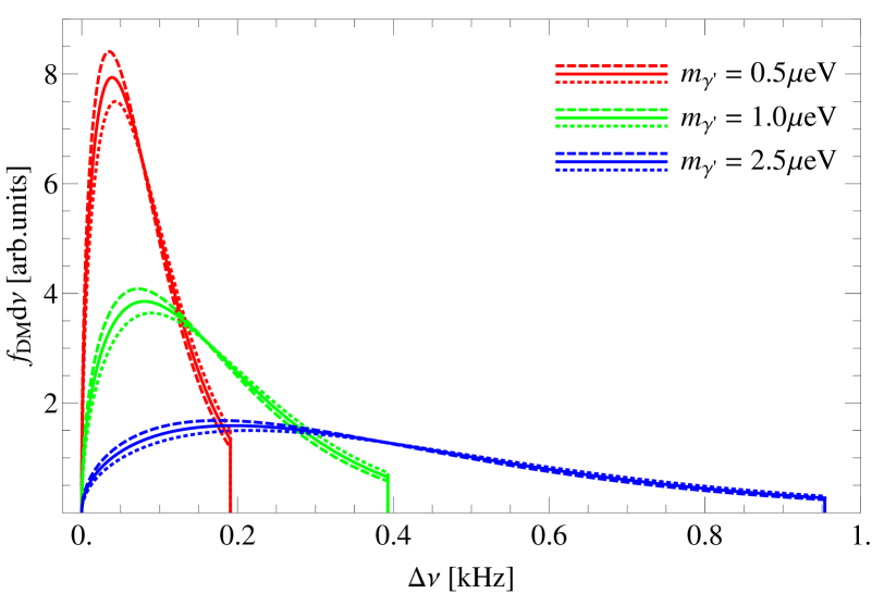
Figure 1: Relative power and distribution of the dark matter conversion signal with respect to the rest-mass frequency at $0.5\text{\,}\mathrm{\SIUnitSymbolMicro eV}$ ($122\text{\,}\mathrm{MHz}$, red), $1.0\text{\,}\mathrm{\SIUnitSymbolMicro eV}$ ($244\text{\,}\mathrm{MHz}$, green), and $2.5\text{\,}\mathrm{\SIUnitSymbolMicro eV}$ ($610\text{\,}\mathrm{MHz}$, blue), calculated assuming the DM velocity truncation at $v_{\mathrm{esc}}=$$530\text{\,}\mathrm{k}\mathrm{m}\,\mathrm{s}^{-1}$. The dashed and dotted lines of respective colors illustrate the maximum effect of yearly modulation of the signal measured on December 2 (dashed) and June 2 (dotted).

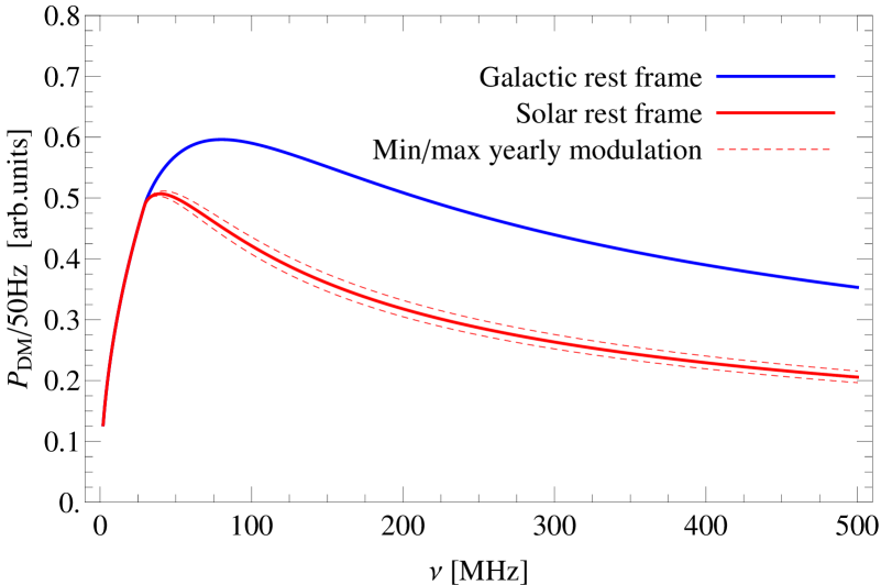
Figure 2: Relative power of DM signal in a single $50\text{\,}\mathrm{Hz}$ channel of WISPDMX as a function of measurement frequency. The peak at $39.8\text{\,}\mathrm{MHz}$ corresponds to the situation when the channel bandwidth of WISPDMX measurements roughly coincides with the bandwidth resulting from the velocity truncation of the DM halo. Above and below this frequency, the channel power is decreasing due to over- and under-resolving the DM signal. For the under-resolved signal at $\nu<$39.8\text{\,}\mathrm{MHz}$$, the channel signal is $\propto\nu^{1/2}$. For the over-resolved part, it depends on the actual shape of the DM velocity distribution.

The relative power of the DM signal received in a single 50 Hz channel of WISPDMX, $P_{\mathrm{DM}}(\nu)=P_{\mathrm{DM}}(\Delta\nu(\Delta u)=50\,\mathrm{Hz})$, is shown in Fig. 2 as a function of the measurement frequency. The power peaks at $\nu=$39.8\text{\,}\mathrm{MHz}$$, at which the channel width of $50\text{\,}\mathrm{Hz}$ roughly corresponds to the bandwidth induced by the velocity truncation in the dark matter halo. Below $39.8\text{\,}\mathrm{MHz}$, the signal power decreases $\propto\nu^{1/2}$, as expected for the case of under-resolving the signal. Above $39.8\text{\,}\mathrm{MHz}$, the DM signal is over-resolved, and its dependence on the measurement frequency is determined by the shape of the DM velocity distribution.

For the over-resolved signal, summing over several frequency bins should improve the sensitivity. The optimum sensitivity achieved with the channel summing is illustrated in Fig. 3 which shows an effective relative sensitivity factor, $G_{\rho}$, for the dark matter signal received in multiple channels of WISPDMX measurements. In the calculations of the sensitivity of WISPDMX measurements, this factor should be applied to modify the value of local dark matter density. The different curves plotted in Fig. 3 illustrate that summing over up to 13 frequency channel is required to achieve a nearly homogeneous sensitivity over the entire $40\text{\,}\mathrm{MHz}500\text{\,}\mathrm{MHz}$ frequency range. The plots shown in Fig. 3 are calculated for $v_{\mathrm{esc}}=530$ km/s. The respective frequency ranges for achieving the optimal sensitivity by summing over a given number of spectral channels are given in Table 1. The effect that the uncertainty in the truncation velocity has on this optimum sensitivity curve is within 10% for the plausible range of $v_{\mathrm{esc}}$ from 450 km/s to 650 km/s.

Figure 3: Sensitivity to the dark matter signal that can achieved with WISPDMX by summing over different numbers of $50\text{\,}\mathrm{Hz}$ spectral channels. The effective relative sensitivity factor $G_{\rho}$ is the ratio of the measurement sensitivity to the maximum sensitivity, calculated for $v_{\mathrm{esc}}=$530\text{\,}\mathrm{k}\mathrm{m}\,\mathrm{s}^{-1}$$. Dashed lines illustrate sensitivities resulting from summing over a fixed number of spectral channels, from one to sixteen. The upper envelope of these curves, plotted in red, describes the sensitivity of WISPDMX to the dark matter signal achieved by summing over the optimum numbers of spectral channels as listed in Table 1.

Table 1: Frequency ranges for optimal sensitivity achieved by summing over $n_{\mathrm{ch}}$ channels of 50 Hz in width.

$n_{\mathrm{ch}}$	Range [MHz]		$n_{\mathrm{ch}}$	Range [MHz]
1	0.0– 59.0		7	263.8–304.8
2	59.0–100.6		8	304.8–345.3
3	100.6–141.6		9	345.3–386.4
4	141.6–182.2		10	386.4–426.9
5	182.2–223.2		11	426.9–468.0
6	223.2–263.8		12	468.0–500.0

3 WISP Dark Matter eXperiment (WISPDMX)

The WISPDMX experiment employs a radio frequency resonant cavity of the type used at the proton accelerator ring designed for the SPS collider and modified for the HERA experiment [29, 30, 31]. A basic scheme of the experiment setup is shown in Fig. 4. The WISPDMX apparatus comprises the following functional groups: mechanical components (the cavity, the plunger assembly, and the driving motors), an amplifier chain, a frequency calibration system, a data acquisition system, and an automated experiment control system. The cavity is tuned with a set of two plungers which are driven by computer controlled electric stepper motors. A custom made data acquisition system provides recording over the entire $500\text{\,}\mathrm{MHz}$ frequency range with a frequency resolution of $50\text{\,}\mathrm{H}\mathrm{z}$. The input voltage signal is digitized in the time domain using a commercial 12-bit analog-to-digital converter (ADC) of the type Alazar ATS 9360. The fast Fourier transformation (FFT) of the digitized output is subsequently carried out with a CUDA based parallel code running on a commercial GPU unit (GTX Titan X). The following subsections will describe the function of each of these groups, with specific details on the development and performance of the individual components.

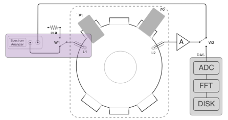
Figure 4: Schematic diagram of the WISPDMX setup, divided into three groups: The Mechanical Components (box with dash-line border) includes the 208 MHz RF cavity, and two tuning plungers $P1$ and $P2$. The Frequency Calibration (the blue shaded box) comprises a radio switch $W1$, a spectrum analyzer, and two loop antennas $L1$ and $L2$ coupled to the cavity. The Acquisition System (the gray shaded box) includes the antenna $L2$, amplifier chain ($A$) with an average gain of 80 dB, an analog-to-digital converter (ADC, Alazar ATS-9360), and a CUDA FFT unit (Nvidia GPU). The antenna $L2$ and the amplifier chain are shared between the calibration system and the acquisition system, using the radio switch $W2$.

3.1 Mechanical Components

The mechanical components of WISPDMX include a $208\text{\,}\mathrm{MHz}$ HERA resonant cavity and a tuning plunger assembly consisting of two plungers as shown in Fig 4. The cavity is made of copper, and it has a diameter of $96\text{\,}\mathrm{cm}$ and volume of $447\text{\,}\mathrm{L}$ [30, 31, 29] (Fig. 5). The inner surface of the cavity is polished to maintain the electromagnetic reflection and achieve a quality factor of $Q_{0}\sim${10}^{4}$$ at a number of resonant modes. The unloaded quality factor can be estimated from the following equation

$$Q_{0}=\frac{\mu_{0}V}{\mu_{c}S\delta_{f}}\,,$$ (3.1)

where $\mu_{0}$ and $\mu_{c}$ describe permeability of vacuum and copper respectively, $V$ and $S$ are the volume and total inner surface of the cavity, and $\delta_{f}$ is the penetrating depth of an electromagnetic wave with a frequency $\nu$.

There are six ports distributed around the cylindrical rim of the cavity. These ports initially used to mount tuning plungers and power couplers when the cavity was operated as a part of particle accelerator. For the WISPDMX setup, two ports are occupied by the tuning plungers, as shown in Fig. 4. The remaining ports are closed. The positioning range of a plunger unit is constrained to be $0\text{\,}\mathrm{mm}110\text{\,}\mathrm{mm}$. The stepper motor (Trinamic QSH6018) which can be driven at a micro-step precision of 1/1600 of revolution is coupled to a gear box and used for positioning the plunger in increments of $0.3\text{\,}\mathrm{\SIUnitSymbolMicro m}$ per micro step. The linear tuning distance of $1\text{\,}\mathrm{mm}$ corresponds to two full revolutions of the gear box. Each of the two stepper motors driving the plungers is monitored by the device control computer which is synchronized with the data acquisition control computer (see also Sect. 3.5).

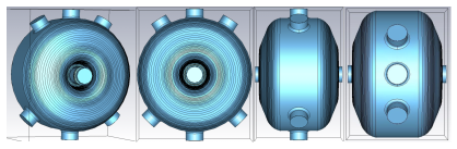
Figure 5: A rendered view of the $208\text{\,}\mathrm{MHz}$ resonant cavity at different orientations. This mechanical model is used with the commercial software package CST^TM [32] to calculate the electromagnetic field configuration of each resonant mode.

3.2 Amplifier chain

The amplifier chain of WISPDMX comprises two WantCom amplifiers, WBA0105B and the WBA0105-45R, providing a total of 79 dB amplification over the $150\text{\,}\mathrm{MHz}500\text{\,}\mathrm{MHz}$ frequency range and an effective noise temperature of 35 K. The cumulative gain of the amplifier chain is shown in Fig. 6. Below 100 MHz, the gain starts to decrease rapidly, but the amplifier chain can be used effectively down to frequencies of $\approx 10$ MHz, thus extending the WISPDMX measurements down to the hidden photon mass of $\approx 0.4$ neV.

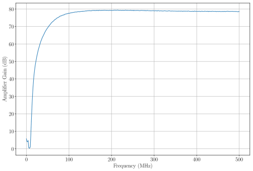
Figure 6: Cumulative gain of the amplifier chain. The nominal $\approx 79$ dB amplification is realized over the $150\text{\,}\mathrm{MHz}500\text{\,}\mathrm{MHz}$ frequency range, and the lowest usable frequency is $\approx 10$ MHz ($\approx 0.4$ neV).

3.3 The Resonant Cavity

To describe and parameterize the performance of the HERA resonant cavity over the entire $0$–$500\text{\,}\mathrm{MHz}$ frequency range, we combined transmission and reflection measurements and numerical simulations of the cavity geometry. Within this range, we have identified ten resonant modes of the cavity (see Table 2). The individual modes have been characterized using a transmission measurement carried out with a spectrum analyzer Rohde-Schwarz FSP 7 outfitted with a tracking function. These measurements provide the resonant frequency and the quality factor of each of the resonant mode.

The form factor of each mode is obtained via equation 2.3, in which the electric field configuration of a given resonant mode is calculated using a numerical simulation of the cavity. The simulation software Computer Simulation Technology is used for calculating the field structure of each resonant mode. The tunable plunger units are included in the simulation as well.

In order to characterize the cavity response to the tuning plungers and to determine the optimal tuning track, both the transmission measurements and the field structure simulations have been made over a 12$\times$12 grid corresponding to all paired combinations of twelve different tuning positions of each plunger equally spaced in the $0\text{\,}\mathrm{mm}110\text{\,}\mathrm{mm}$ tuning range. At each individual step of the simulation, the plunger positions are modified accordingly, and the field configuration and the form factor are calculated for each of the modes studied.

The resulting optimal tuning track is achieved by starting both plungers at the zero position, then driving one of the plunger over its full $110\text{\,}\mathrm{mm}$ range, and then driving the second plunger over the full tuning range (the actual choice of the order in which the plungers are driven does not affect the tuning range and speed, owing to the similarity in the plungers positions and orientations with respect to the main axes of symmetry of the cavity).

The derived tuning response of the cavity is summarized in Table 2, in which ten resonant modes identified at frequencies below $500\text{\,}\mathrm{MHz}$ are listed together with their calculated form factors and measured resonant frequencies.

Based on these calculations, we have selected four modes which have non-zero form factors at all plunger positions and thus are best suitable for our measurements. The four selected modes are $\text{TM}_{010}$, $\text{TE}_{111-1}$, $\text{TE}_{111-2}$, and $\text{TM}_{020}$.

The measured changes of the resonant frequencies of these four resonant modes for the full range of plunger positions used for the tuning are shown in Fig. 7. The plot shows that the four resonant modes cover frequency ranges from $\Delta\nu\approx$1\text{\,}\mathrm{MHz}$$ for the fundamental mode and up to $\Delta\nu\approx$6\text{\,}\mathrm{MHz}$$ for the TE_111-2 mode. The combined frequency range covered by the four modes is $\approx$10\text{\,}\mathrm{MHz}$$. The ground mode is tuned at a rate of $\approx$5\text{\,}\mathrm{k}\mathrm{H}\mathrm{z}\mathrm{/}\mathrm{m}\mathrm{m}$$, over the full range of the plunger tuning. The fastest tuning rate of about $-60\text{\,}\mathrm{k}\mathrm{H}\mathrm{z}\mathrm{/}\mathrm{m}\mathrm{m}$ is achieved for the TE_111-2 mode, in the range of $50\text{\,}\mathrm{mm}90\text{\,}\mathrm{mm}$ of the second plunger. Thus, WISPDMX can achieve an accuracy of frequency tuning of better than $1.5\text{\,}\mathrm{Hz}20\text{\,}\mathrm{Hz}$ per tuning step, depending on the resonant mode.

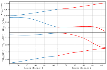
Figure 7: Tuning ranges of the resonant frequencies of the four cavity modes corresponding to the tuning scheme adopted for the WISPDMX measurements. The two transverse magnetic modes, TM₀₁₀ and TM₀₂₀ are tuned at nearly constant rates of $\approx$5\text{\,}\mathrm{k}\mathrm{H}\mathrm{z}\mathrm{/}\mathrm{m}\mathrm{m}$$ and $\approx$20\text{\,}\mathrm{k}\mathrm{Hz}\mathrm{/}\mathrm{m}\mathrm{m}$$, respectively. The two TE₁₁₁ modes are weakly tuned over most of the plunger ranges, and show the approximate highest tuning rates of $-45\text{\,}\mathrm{k}\mathrm{H}\mathrm{z}\mathrm{/}\mathrm{m}\mathrm{m}$ (TE_111-1, for plunger 1 range of $60\text{\,}\mathrm{mm}100\text{\,}\mathrm{mm}$) and $-60\text{\,}\mathrm{k}\mathrm{H}\mathrm{z}\mathrm{/}\mathrm{m}\mathrm{m}$ (TE_111-2, for plunger 2 range of $50\text{\,}\mathrm{mm}90\text{\,}\mathrm{mm}$).

Following these considerations, a tuning step of $10\text{\,}\mathrm{\SIUnitSymbolMicro m}$ is selected for the WISPDMX measurements, thus requiring a total of $22\,000$ steps to scan over the full range of the two plungers. At this tuning step, the resonant modes are sampled at frequency steps ranging from $50\text{\,}\mathrm{Hz}$ for the ground mode TM₀₁₀ (corresponding to $\approx$1% of its resonance width) to $610\text{\,}\mathrm{Hz}$ (or $\approx$10% of the resonance width) for the fastest tuning rate of the TE_111-2 mode. Thus, the accuracy WISPDMX measurements will not be affected by the frequency profiles of the resonant modes.

The resulting frequency steps for both TM modes constitute 25% and 36% of the respective DM signal width, hence the selected tuning step will not affect the measurement sensitivity for these modes. The same is true about the TE₁₁₁ mode, except for the ranges of its high tuning rates where the tuning step in frequency reaches 100% and 150% (for TE_111-1 and TE_111-2, respectively) of the expected width of the DM signal. However, even for these tuning steps, the sensitivity reduction would be within 10%. Hence the selected plunger tuning step of $10\text{\,}\mathrm{\SIUnitSymbolMicro m}$ is adequate for scanning the frequency ranges covered by the four resonant modes used in WISPDMX.

The tuning of the plungers changes both the frequency as well as the field configuration inside the cavity. Therefore, the tuning may lead to a change of form factor (see e.g., the form factor of the $\text{TM}_{011}$ where the deformation of the field structure leads to an increase of the form factor when both plungers are fully extending into the cavity). However, the form factors of the four modes selected above vary only weakly with changing the position of the plungers.

It should be mentioned that both the simulations and the transmission measurements have indicated that the peak frequencies of some of the resonant modes have crossed in the course of the tuning over the full range of the plungers. However, none of the four modes selected for making the WISPDMX measurements suffers from this mode crossing, as can be seen from Fig. 7.

Table 2: Characteristics of the HERA cavity at different plunger positions

Mode:	Plunger position (0; 0)			Plunger position (110; 0)			Plunger position (110; 110)
	$\nu_{0}$	$Q_{0}$	$\cal{G}$	$\nu_{0}$	$Q_{0}$	$\cal{G}$	$\nu_{0}$	$Q_{0}$	$\cal{G}$
TM010	207.99	53542	0.433	208.53	52395	0.431	209.06	51281	0.429
TM011	314.87		0.000	308.60		0.090	305.75		0.112
TE111-1	321.69	62067	0.679	318.13	55253	0.522	316.48	54482	0.504
TE111-2	322.69	62074	0.679	323.20	60431	0.677	319.21	54017	0.605
TM110-1	390.99		0.000	391.85		0.035	359.68		0.053
TM110-2	392.28		0.000	393.37		0.000	390.37		0.011
TE210-1	397.84		0.000	382.28		0.000	399.08		0.000
TE210-2	399.02		0.000	401.24		0.000	401.33		0.001
TM020	455.07	47902	0.321	456.92	46888	0.323	458.87	45739	0.324
TM012	461.73		0.000	457.33		0.018	449.94		0.009

Notes: Resonant frequencies, $\nu_{0}$, and geometrical form factors $\mathcal{G}$ of ten resonant modes of the HERA cavity identified in the $500\text{\,}\mathrm{MHz}$ range. The mode parameters are evaluated at three different plunger positions: the initial $(0;\,0)$ position with both plungers fully retracted, the $(110;\,0)$ position with one of the plungers extended by $110\text{\,}\mathrm{mm}$ into the cavity, and the $(110;\,110)$ position with both plungers fully extended into the cavity. Four modes with form factors close to unity (highlighted in boldface) are selected for the WISPDMX measurements. For these modes, the respective quality factors, $Q_{0}$, are also listed.

3.4 Calibration Procedures

In order to monitor and calibrate the performance of the WISPDMX apparatus, several procedures are carried out at each tuning step of the measurement.

3.4.1 Broadband gain

With the four resonant modes identified in Sect. 3.3 as suitable for hidden photon searches, the broadband gain of WISPDMX can be calculated using Eqn. 2.5. This calculation is performed at each tuning step of the measurements. An example of the broadband gain calculated for a single position of the plunger assembly is shown in Fig. 8.

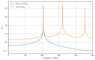
Figure 8: The total cumulative gain $g(\nu)$ of the four relevant resonant modes of WISPDMX at the plunger assembly position (0, 110), calculated using Eqn. 2.5. The contribution of the fundamental mode $\textrm{TM}_{010}$a is shown with a blue line.

3.4.2 Monitoring of the resonances

In addition to the changes of the resonant response of the cavity resulting from the tuning, variable ambient conditions (temperature, air pressure) lead to variations of the resonant frequencies (the changes of the respective quality factors and form factors are negligible). In Fig. 9, we show a typical day-night cycle in the laboratory during which the temperature drops by about $\Delta T\approx$2\text{\,}\mathrm{\SIUnitSymbolCelsius}$$. This leads to an increase of the resonant frequencies of the four modes by $\Delta\nu(\mathrm{TM}_{010})\approx$7\text{\,}\mathrm{kHz}$$ up to $\Delta\nu(\mathrm{TM}_{020})\approx$16\text{\,}\mathrm{kHz}$$ with $\Delta\nu_{i}/\nu_{i}\propto-\Delta T/T$, as expected for a self-similar thermal contraction of the cavity.

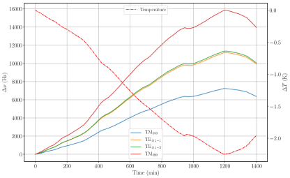
Figure 9: Change of the resonant frequencies of the four selected modes induced by the decrease and increase of the ambient temperature. The change of the cavity volume with decreasing/increasing room temperature results in reciprocal changes of the frequencies of the resonant modes.

A frequency calibration system is therefore necessary in order to monitor the resonant frequencies during the experimental measurements. The frequency calibration measurements are performed intermittently (at intervals short enough to warrant interpolation of the resonant frequencies and quality factors), each time after a series of data taking and tuning steps. The calibration procedure uses measurements of the transmission coefficient of the network which contains the resonant cavity. The transmission coefficient is measured by sending a feed signal and recording the output with the spectrum analyzer.

The spectrum analyzer (RS FSP7 with tracking option) is connected to two loop antennas ($L1$ and $L2$, in Fig. 4), so that the tracking generator feeds the antenna $L1$ and the spectrum analyzer receives the feedback output signal from the antenna $L2$. The output from $L2$ can be switched by the radio switch $W2$ between the input of the spectrum analyzer or the ADC of the acquisition system. The tracking generator connected to the antenna $L1$ sweeps the preselected frequency interval of $300\text{\,}\mathrm{kHz}$ around the resonant frequency of a given mode, sending a signal with a power of $-10\text{\,}\mathrm{dBm}$ and a spectral resolution of $\Delta\nu=$300\text{\,}\mathrm{Hz}$$.

From the output registered at the antenna $L2$, the central resonant frequency and the loaded quality factor are determined by fitting a characteristic Lorentzian function given by

$$P_{\mathrm{res}}=\frac{h}{1+4Q^{2}(\frac{\nu}{\nu_{0}}-1)^{2}},$$ (3.2)

where $P_{\mathrm{res}}$ is the power recorded by the spectrum analyzer, $\nu_{0}$ and $Q$ are the resonant frequency and quality factor, respectively. The scaling parameter $h$ is proportional to the strength of the input signal. A least square fit is used to estimate the values of these three parameters and their uncertainties. The fit yields a good agreement with the measurement as illustrated in Fig. 10.

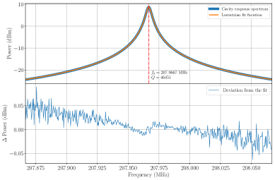
Figure 10: Example of a Lorentzian profile fit to the transmitted power recorded near the resonant frequency of the $\text{TM}_{010}$ mode. The bottom panel shows the post-fit residual power.

3.4.3 Reference frequency

The overall accuracy of the frequency calibration may depend also on the systematic uncertainty and drifts of the reference frequency of the spectrum analyzer. The reference frequency can drift over time and with changing temperature conditions. The temperature in the laboratory changes by as much as $2\text{\,}\mathrm{\SIUnitSymbolCelsius}$. The spectrum analyzer was calibrated by the manufacturer in December 2016, and the frequency measured with the spectrum analyzer has a systematic uncertainty at the level of ${10}^{2}\text{\,}\mathrm{Hz}$, taking into account that for the Rohde-Schwarz FSP 7, the relative aging rate $\dot{\nu}=${10}^{-6}\text{\,}{\mathrm{yr}}^{-1}$$ and the relative frequency drift per $\mathrm{\SIUnitSymbolCelsius}$ is ${10}^{-6}$. In addition to the systematic uncertainty, we estimate the statistical uncertainty from the fitting of the Lorentzian function 3.2 to be lower than $1\text{\,}\mathrm{Hz}$ (see also Fig. 10). As all these factors are substantially smaller than the intrinsic systematic uncertainty of the reference frequency, we take $\sigma_{\nu}=${10}^{2}\text{\,}\mathrm{Hz}$$ as the total frequency accuracy of our measurements. This corresponds to an error of $\sigma_{\mathrm{m}}=$0.4\text{\,}\mathrm{peV}$$ for the hidden photon mass, and hence this uncertainty would not affect the present WISPDMX measurements. It may however become a potentially adverse issue if one would attempt to increase the signal-to-noise ratio of the resonant detection by summing multiple independent measurements.

3.4.4 Antenna coupling

A network analyzer, Anritsu 37369A, is connected to the loop antenna $L2$ to measure the coupling, $\kappa$, of the antenna to the cavity over the entire measured bandwidth. The coupling is derived using the $S_{11}$ reflection parameter, with

$$\kappa=\frac{1-|S_{11}|}{1+|S_{11}|}\,.$$ (3.3)

The measured antenna coupling of the WISPDMX setup is shown in Fig. 11. The WISPDMX antenna is weakly coupled to the cavity, with $\kappa\ll 1$ over the entire bandwidth. Our measurements indicate that the coupling is not sensitive to the cavity tuning, and it varies within less than 5% over the entire range of the plunger positions. We apply therefore a single $\kappa(\nu)$ profile for evaluating all of the WISPDMX measurements.

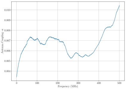
Figure 11: The coupling factor, $\kappa(\nu)$, of the antenna used for the WISPDMX measurements.

3.5 Data Acquisition System

The data acquisition system (DAS) of WISPDMX provides real time recording at a rate of $1\text{\,}\mathrm{GS}\text{\,}{\mathrm{s}}^{-1}$, corresponding to a maximum recording bandwidth of $500\text{\,}\mathrm{MHz}$. The system contains two main components: a 12-bit analog-to-digital converter (ADC), modified for performing a high volume continuous streaming to the host memory, and a high-power CUDA GPU employed for carrying out the FFT and related operation (e.g., array adding and converting).

The DAS can presently accumulate up to $10\text{\,}\mathrm{s}$ of continuous sampling in the time domain, hence it can principally achieve a spectral resolution of $0.1\text{\,}\mathrm{Hz}$ over the entire $500\text{\,}\mathrm{MHz}$ band. However, storing a high-resolution broadband spectrum leads to prohibitively long dead times for the pipeline processing, data I/O and storage. As a compromise between increasing the spectral resolution and reducing the dead time, the $10\text{\,}\mathrm{s}$ of data are broken down into 500 segments of $0.02\text{\,}\mathrm{s}$ in duration, and the FFT is applied to each of these segments. The resulting broadband spectrum has then a spectral resolution of $50\text{\,}\mathrm{Hz}$. After the FFT, the resulting 500 spectra are co-added to calculate the average spectrum. After the averaging, the noise in the averaged spectrum is $\sigma_{\text{a}}=\sigma_{1}/\sqrt{N}$, where $\sigma_{1}$ is the noise power of a single spectrum and $N$ is the number of spectra used in the averaging process. The noise improvement achieved by the averaging of the individual spectra is illustrated in Fig. 12.

Figure 12: Examples of broadband spectra from the acquisition system illustrating the noise reduction achieved by spectral averaging. Blue: single spectrum from $0.02\text{\,}\mathrm{s}$ of data-taking. Green: average of 100 single spectra. Red: average of 500 single spectra. The latter is the output spectrum for each acquisition step of WISPDMX.

A scheme of the WISPDMX data acquisition and processing procedures is presented in Fig. 13. At each data acquisition step, the ADC streams the data directly into the host memory grid, splitting the data stream into $1000$ individual buffers each holding $10\text{\,}\mathrm{MS}$ ($0.01\text{\,}\mathrm{s}$) of data. Once the first $1000$ buffers are stored in the host computer, the ADC starts recording the next $10\text{\,}\mathrm{s}$-segment of data and streams it to the second memory grid. In parallel to the data taking, the recordings from the first memory grid are transferred to the GPU. Inside the GPU, each two consecutive $10\text{\,}\mathrm{MS}$ buffers are merged to create $500$ buffers containing $20\text{\,}\mathrm{MS}$ time series arrays. Each individual $20\text{\,}\mathrm{MS}$ array is then Fourier transformed, yielding a power spectrum with 10 million spectral channels (10 MC spectrum, in Fig. 13) with a $50\text{\,}\mathrm{Hz}$ frequency resolution. The resulting 10 MC power spectrum is moved to the second memory grid.

After all 500 spectra have been transferred to the second memory grid, the average spectrum is calculated as the final output of the DAS for a $10\text{\,}\mathrm{s}$ integration time corresponding to a single step of the WISPDMX measurement run.

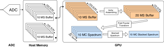
Figure 13: Detail of the DAS operations, illustrating the multi-threading and memory management employed to process individual 10-megasamples (10 MS) time series recordings into 10-megachannels (10 MC) power spectra. The GPU executes three main CUDA-powered functions: the buffer assembling, the CUDA-FFT, and the spectrum stacking.

With the application of multi-threading and memory managing, the computational processes inside the GPU are completed in less than $3.2\text{\,}\mathrm{s}$ in total, (see the time breakdown in Table 3). During this time, a tuning step ($\approx$$0.1\text{\,}\mathrm{s}$) and the ADC initialization for the next acquisition ($\leq$$2.8\text{\,}\mathrm{s}$) are performed in parallel. The combined ADC and GPU acquisition system has therefore a fractional dead time of less than $30\text{\,}\mathrm{\char 37\relax}$. In order to improve this performance and achieve near real-time acquisition operations, it would be required both to use multiple GPUs and to reduce the initialization time of the ADC before each data acquisition. However, this initialization time is a design limitation of the commercial ADC broad.

Table 3: Chronological breakdown of a single data acquisition step

Component	Process	Time ($\mathrm{s}$)
ADC	Initialization of acquisition	1.2 – 2.8
	Filling host memory	10.002
GPU	Data transfer from host memory to GPU	2.0509
	Buffer assembling	0.21
	CUDA-FFT	0.841
	Spectrum stacking	0.163
	Copying stacked spectrum to host	0.008
Host	Saving stacked spectrum to disk	0.04

Note: The processes in the GPU and the Host are run in parallel with the ADC processes, which enables performing near real-time data acquisition.

3.6 WISPDMX data taking and calibration procedure

In order to make automated measurements at each of the $22\,000$ tuning steps planned for WISPDMX data taking run, the three main components of WISPDMX described above are combined in a connected and synchronized setup controlled by two dedicated computers: the mechanical and frequency calibration controller managing the plunger tuning, frequency calibration system, and radio switches, and the acquisition and signal digitizer controller operating the DAS. A scheme of the operational structure of WISPDMX measurements is shown in Fig. 14.

The WISPDMX operations are ultimately structured into multiple measurement cycles. Each measurement cycle begins with a frequency calibration step (lasting for about $4\text{\,}\mathrm{s}$). Subsequently, the data acquisition system acquires data for the current setting of the plunger assembly, and then the plunger assembly is moved to the next tuning position. These two operations are repeated ten times, before proceeding to the next measurement cycle. The output of both the frequency calibration module and the data acquisition system is stored on a local hard drive for offline processing and analysis. The respective dead time for a single WISPDMX measurement cycle is less than $30\text{\,}\mathrm{\char 37\relax}$.

The typical total duration of a single measurement cycle is $\leq$$133\text{\,}\mathrm{s}$. Within this time, the potential frequency drifts due to the temperature changes should be $\leq$$40\text{\,}\mathrm{Hz}$, for the worst measured temperature gradient ($\approx$$0.14\text{\,}\mathrm{K}\mathrm{/}\mathrm{h}\mathrm{r}$, see Fig. 9) and the most temperature-sensitive TE₁₁₁ mode. Thus even the maximum expected frequency drift should be smaller than the frequency resolution of the measurements, and it can be adequately represented by a linear interpolation between two successive frequency calibration steps.

With the tuning step of $10\text{\,}\mathrm{\SIUnitSymbolMicro m}$, the accumulated shift between two runs of the frequency calibration amounts to $100\text{\,}\mathrm{\SIUnitSymbolMicro m}$. This corresponds to a maximum possible frequency change of $6\text{\,}\mathrm{kHz}$, within which the frequency changes are well described by a linear interpolation. The same considerations apply to the quality factors and mode coupling factors of the modes. Hence, the parameters of the resonant modes are linearly interpolated, in order to obtain the calibration information for each of the tuning steps performed between these two calibration measurements.

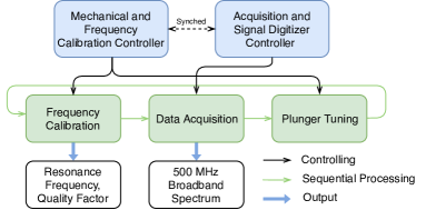
Figure 14: Operational scheme of WISPDMX measurements. The Control Module (top row) drives the Executive Module (middle row) which produces the science and calibration output data (bottom row). The Control Module synchronizes the operations of the mechanical, frequency calibration, and data acquisition controllers. A measurement cycle begins with engaging the Frequency Calibration block which determines the actual parameters of the resonant modes. The Data Acquisition block is then initialized and set to record 10 seconds of data. After the recording has been completed, the Control Module first engages the Plunger Tuning block to move the plunger to a new tuning position (while transferring the recorded data to the GPU for further processing) and then proceeds to performing the next round of data acquisition. The data acquisition and plunger tuning steps are repeated ten times before starting the next measurement cycle which begins with execution of another frequency calibration procedure.

4 WISPDMX First Science Run

The measurements comprising the first science run of WISPDMX were made during the time period from 23rd October 2017 to 2nd November 2017, comprising a total of $22\,000$ spectra, each produced from a single $10\text{\,}\mathrm{s}$ data taking and tuning step. The first science run of WISPDMX had been carried out using a weakly coupled antenna.

In the course of the measurements, the two plungers were consecutively extended into the cavity, advancing at a rate of $10\text{\,}\mathrm{\SIUnitSymbolMicro m}$ per tuning step. The complete run has been accomplished within $8$ sub-runs, with each sub-run providing $2000$ or $3000$ acquisitions. The total acquisition time ($$22\,000$\times$10\text{\,}\mathrm{s}$$) corresponds to $2.46\text{\,}\mathrm{d}$ of data. The remaining time ($\sim 7$ days) comprised various auxiliary processes and activities, including a remaking of one sub-run because of a memory jam in the ADC, frequency calibration, plunger tuning, and electronic switch operation, and a break between two sub-runs. For the first science run, WISPDMX was operated at the room temperature of $20\pm 1.\text{\,}\mathrm{\SIUnitSymbolCelsius}$. The frequency calibration procedure was invoked after every 10 consecutive data recording and tuning steps. For the offline analysis, the resonant frequencies and quality factors of the resonant modes are extracted from the sweep spectra provided by the frequency calibration procedure.

4.1 Single Acquisition Spectra

Visually, the $22\,000$ single acquisition spectra from the first science run of WISPDMX have a similar power level and spectral bandpass. The first and the last spectrum recorded over the course of the first science run are shown in the two panels of Fig. 15, demonstrating the stable broadband spectral profile. The broadband spectrum in the range below $\approx$$100\text{\,}\mathrm{MHz}$ is affected by the rapidly decreasing gain of the amplifier chain. In addition to this effect, there are several prominent and time-dependent noise peaks present in the spectrum. These noise peaks originate most likely from interference produced by one or several devices used in the measurements (e.g., the amplifiers, the radio switches, or the ADC clock) or from stray fields that penetrate the cavity, even though the cavity provides strong shielding. The stray noise may penetrate through the shielded coaxial cables, the coaxial connectors, and the unshielded amplifier box. The narrow band noise is subsequently amplified before recording it with the ADC. During the first science run, we did not have the capacity to fully investigate and eliminate the origins of these spurious features. Fortunately, most of them reside in the off-resonance regions of the measured spectrum and cover multiple channels, and hence they can be easily mitigated and excluded from the analysis. These prominence of these interference signals should be reduced during the planned subsequent runs of WISPDMX which will be carried out with an improved setup and better radio shielding.

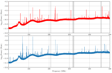
Figure 15: Power spectra obtained from the first (top) and the last (bottom) 10-$\mathrm{s}$ acquisitions of the WISPDMX measurements made at the initial and the final positions of the two plungers, respectively. The shaded areas in the panels indicate the tuning ranges of the resonant modes achieved during the science run.

4.2 Averaged Spectrum

To search for DM signal outside of the ranges covered by the four tuned resonant modes, the averaged spectrum is generated from the $22\,000$ single acquisition spectra. Similarly to the thermal noise reduction achieved by the averaging process described in Sect. 3.5, averaging of the single acquisition spectra results in reducing the fluctuations by a factor of $1/\sqrt{$22\,000$}$. This is demonstrated in Fig. 16, where the averaged spectrum and the single acquisition spectrum are compared. The expected reduction of the fluctuations in the power level is clearly visible there. Apart from this reduction of the noise fluctuation, the average spectrum is otherwise very similar in its shape and power level to the single acquisition spectrum.

4.3 Signal Scan

We scan both the $22\,000$ single acquisition spectra as well as the composite average spectrum, in order to search for a potential hidden photon signal. The signal scan is performed in two separate steps:

• resonant scan, using single acquisition spectra to search for signals within a narrow bandwidth centered at the respective resonant frequencies of the cavity modes;

• broadband scan, using the average spectrum to search for signals outside of the frequency ranges covered by the cavity tuning.

At each step of this analysis, we assess the noise properties, identify potential candidates, evaluate their significance, and calculate the specific power at which a signal can be excluded. For the signal scan in the resonant part of the spectrum, three a priori defined consecutive selection criteria are applied:

1. Choosing a region of interest (ROI) which is centered at the frequency $\nu_{0}$ of the resonance and has a bandwidth of $100\text{\,}\mathrm{kHz}$ $\text{ROI}=[\nu_{0}-$50\text{\,}\mathrm{kHz}$,\nu_{0}+$50\text{\,}\mathrm{kHz}$]$. The significance level $\mathcal{S}$ in one channel is given by

   $$\mathcal{S}=\frac{S}{\sigma}=\frac{P_{\text{1 channel}}-\mu_{\text{ROI}}}{\sigma_{\text{ROI}}}\,,$$ (4.1)

   with $\mu_{\text{ROI}}$ and $\sigma_{\text{ROI}}$ are the mean power and noise power of the ROI respectively which are calculated using the power level of the channels located in the ROI. If the power excess $S$ in a channel (within the ROI) has a significance $\mathcal{S}>3$, the channel is recorded and becomes a level-I signal candidate.

2. Tracking the position and amplitude of the level-I candidate signal in multiple consecutive spectra: The position of the candidate signal must reside in the same channel while their amplitude must vary while the position of the resonant frequency changes in the tuning procedure. The candidate which satisfies both conditions becomes a level-II candidate.

3. Test the signal width condition on the level-II candidate: if the number of consecutive level-II channels is equal to the expected signal width of the signal in the designated frequency, the level-II candidates are promoted to level-III candidates. Their position is recorded for manual inspection.

In the narrow band searches over the on-resonance region, we are selecting candidates both exactly on-resonance as well as slightly off-resonance. The criterion for the level-II candidates introduced above takes into account that the spectral resolution largely over-samples the width of the resonance. Following that requirement, a true signal can be reliably discriminated against spurious noise.

The broadband signal search is performed using the averaged spectrum. The conditions applied for the broadband search are limited to satisfying the abovementioned criteria of significance (1) and signal width (3), and the search proceeds as follows:

1. Channel search (similar to the on-resonance scan): The list of channel candidates is retrieved after dividing the broadband spectrum into $500$ ROIs with $1\text{\,}\mathrm{MHz}$ width and selecting the channels which exceed the significance threshold of $5$ $\sigma$.

2. Similarly to the third step in the resonant search, the signal width condition is applied to select signals with consecutive channels with a combined width as expected for a dark matter signal at that particular frequency.

It should be noted that the signal scan on the averaged spectrum shares many mutual features between the on- and off-resonance scan algorithm at a single spectrum level. However, the broadband scan performed on the single averaged spectrum is inherently less restrictive on identification of potential candidates because there are no other spectra to compare (and so there is not an equivalent of the level-II criterion to be used for the broadband search in the off-resonance frequency range). In this case, the signal width criterion becomes the most important condition for filtering out spurious candidates.

5 Results

5.1 Detectable Power and the Noise Power

The signal scan procedures described above consider a narrow band excess power in a ROI to be signal-like if it is significant in comparison with the fluctuations of the background spectrum and if it matches the expected line width at the given frequency. The measured broadband spectrum (see Fig. 16) is dominated by the thermal noise of the antenna, the cavity walls and (mostly) narrow band ambient RF noise that couples into the cable connecting the antenna to the amplifier. Additionally, the amplifier contributes to the noise (with the given noise figure of $0.518\text{\,}\mathrm{dB}$). At the digitization step, a negligible amount of noise is added to the overall background (the $12$-bit digitization of the $\pm$0.4\text{\,}\mathrm{V}$$ range introduces a digitization noise power at the level of $-14\text{\,}\mathrm{dBm}$).

In the following, we combine the recorded power spectra and the amplifier gain to estimate the measured poer at the antenna resulting from the WISPDMX measurements and to determine the detectable excess power. As described in Sect. 3.2, the amplifier gain been measured by sending a sweeping signal from the frequency generator to the amplifier chain and recording the output power. The resulting frequency dependent gain presented in Fig. 6 is applied to the recorded WISPDMX power spectra to calculate the measured power spectra as illustrated in Fig. 16. These power spectra are subsequently used for estimating the values of $\mu_{\mathrm{ROI}}$ and $\sigma_{\mathrm{ROI}}$ introduced in Eqn. 4.1.

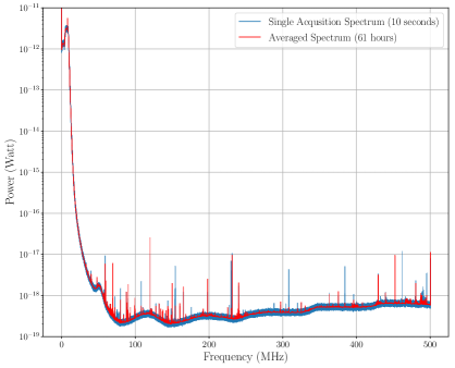
Figure 16: The measured power at the antenna obtained in a single acquisition spectrum (gray) and after averaging the $22\,000$ individual spectra (red) from the WISPDMX first science run.

The channel-by-channel fluctuation $\sigma_{\text{single}}$ of the single spectrum is calculated by collecting the channel power from $22\,000$ single spectra. The $\sigma_{\text{single}}$ is the standard deviation of the collection. While the noise power of the averaged spectrum $\sigma_{\text{averaged}}$ is estimated from the $\sigma_{\text{single}}$ by:

$$\sigma_{\text{averaged}}=\frac{\sigma_{\text{single}}}{\sqrt{$22\,000$}}\,,$$ (5.1)

as mentioned in Sect. 4.2. The noise power at the level of the single spectrum and averaged spectrum are $\sigma_{\mathrm{single}}\sim$8\text{\times}{10}^{-19}\text{\,}\mathrm{W}$$ and $\sigma_{a}\sim$5\text{\times}{10}^{-22}\text{\,}\mathrm{W}$$.

5.2 Results from the Signal Scan

The resonant scan applied to the narrow band frequency intervals selected in the single acquisition spectra around the resonant cavity modes covers the following ranges of the particle mass $0.8602\text{\,}\mathrm{\SIUnitSymbolMicro eV}0.8646\text{\,}\mathrm{\SIUnitSymbolMicro eV}$ ($\text{TM}_{010}$), $1.3088\text{\,}\mathrm{\SIUnitSymbolMicro eV}1.3358\text{\,}\mathrm{\SIUnitSymbolMicro eV}$ ($\text{TE}_{111-1}$, $\text{TE}_{111-2}$), and $1.8820\text{\,}\mathrm{\SIUnitSymbolMicro eV}1.8977\text{\,}\mathrm{\SIUnitSymbolMicro eV}$ ($\text{TM}_{020}$). The resulting number of level-I signal candidates reaching the significance level larger than 3 ($\mathcal{S}>3$) varies between 5 to 8, in a single ROI with $\Delta\nu=$100\text{\,}\mathrm{kHz}$$. The level-I candidates are subsequently filtered using the position and amplitude test performed in the consecutive spectra. However, none of these level-I candidates pass the test on the expected variation of amplitude while tuning across the resonance. On the other hand, the level-I candidates are filtered using the line width test. Compliance with the expected line width of the hidden photon signal requires 5 consecutive channels with an excess for the $\text{TM}_{010}$ mode, 8 consecutive channels for the twin modes $\text{TE}_{111}$, and 11 consecutive channels for the $\text{TM}_{020}$ mode. In our data, there are no such features, as none of the regions with the respective numbers of consecutive channels has a significance level of $\mathcal{S}>2$. This allows us to conclude that the resonant scan searches do not detect any candidate for the hidden photon signal above the level of $2\sigma_{\text{single}}$.

The broadband scan procedure applied to the average spectrum yields a total of $20\,646$ single-channel candidates with significance level larger than 5$\sigma_{\text{averaged}}$. The signal width condition is applied again to filter out the candidates and reduces the total number of candidates down to 642 candidates, together covering a total of 1628 channels.

Table 4: Number of candidates from the broadband scan satisfying the signal line width condition

Width	Range	Candidate	Width	Range	Candidate
(channel)	$\mathrm{MHz}$	level-II	(channels)	$\mathrm{MHz}$	level-II
1	0 - 59.059	280	7	263.763 - 304.804	9
2	59.059 - 100.600	158	8	304.804 - 345.345	1
3	100.600 - 141.641	84	9	345.345 - 386.386	15
4	141.641 - 182.182	31	10	386.386 - 426.926	5
5	182.182 - 223.223	20	11	426.926 - 467.967	6
6	223.223 - 263.763	27	12	467.967 - 500	6

The Table 4 lists the number of these candidates falling within the specific frequency ranges as determined by the expected width of the hidden photon signal. As discussed in Sect. 2.2, the signal is expected to follow the Maxwellian distribution. In a follow-up test the signal candidates are fit with a Maxwellian signal function [20]. The fit is only feasible for the candidates where the expected signal width is resolved across at least five channels. The frequency range used for the fit is extended up to adjacent 10 channels to estimate the background and to include the tail of the Maxwellian function.

The goodness-of-fit criterion is based upon the $\chi^{2}$ calculated with the error given by the noise power of the averaged spectrum. Most of the candidates can be rejected given the large $\chi^{2}$ values found for the given number of degrees of freedom and therefore small $p$-values. The candidate with the largest $p$-value of 8.175% is shown in Fig. 17. For this candidate, five channels are estimated to have a significance level larger than 5, and the central frequency obtained from the fit is $218.017395(^{+9}_{-34})$ $\mathrm{MHz}$.

This rest mass frequency corresponds to a particle mass of $0.90164783(^{+4}_{-14})$ $\mathrm{\SIUnitSymbolMicro eV}$. The fitted width of the Maxwellian profile corresponds to a dark matter halo velocity dispersion of $330^{+70}_{-60}$ $\mathrm{k}\mathrm{m}\mathrm{/}\mathrm{s}$, which agrees well with the observational estimates [21, 22]. If the total excess power of $(1.8\pm 0.2)\times 10^{-21}$\mathrm{W}$$ measured in the fitted profile is produced by the kinetic mixing of the hidden photons from the Galactic dark matter halo, the resulting coupling constant is $(1.1\,^{+0.6}_{-0.2})\times 10^{-12}$, which places it well within the ranges allowed for the hidden photon cold dark matter (see, [5, 6]).

However, further inspection of a broader spectral range around this peak reveals its potential connection to a periodic feature appearing throughout a substantial portion of the spectrum at intervals close to $333.36\text{\,}\mathrm{kHz}$, which are likely an instrumental effect (e.g., an interference signal from the clock of the ADC module). None of these quasi-periodic features has satisfied our selection criteria for a signal candidate, with most of them being limited to two spectral channels. We conclude nevertheless that the nature of this candidate signal needs to be further investigated with additional measurements that can be used to identify potential instrumental effects and to look for the annual modulation expected for the actual dark matter signal.

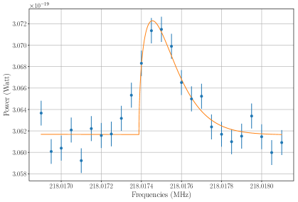
Figure 17: A potential candidate signal with the largest $p$-value (8.175%) of the fit by the Maxwellian profile.The reduced $\chi^{2}$ parameter of the fit is 1.44, calculated for 22 degrees of freedom. The fitted rest mass frequency of $218.017395(^{+9}_{-34})$ $\mathrm{MHz}$ corresponds to a particle mass of $0.90164783(^{+4}_{-14})$ $\mathrm{\SIUnitSymbolMicro eV}$. The width of the fitted profile translates into a dark matter halo velocity dispersion of $330^{+70}_{-60}$ $\mathrm{k}\mathrm{m}\mathrm{/}\mathrm{s}$. If the total excess power of $(1.8\pm 0.2)\times 10^{-21}$\mathrm{W}$$ in the fitted profile is produced by the kinetic mixing of the hidden photons from the Galactic dark matter halo, the resulting coupling constant is $(1.1\,^{+0.6}_{-0.2})\times 10^{-12}$.

5.3 Exclusion Limit from the First Science Run

Leaving the investigation of the potential signal candidate at $218.017\,395\text{\,}\mathrm{MHz}$ to further dedicated measurements, we proceed here to derive limits on the coupling parameter $\chi$ over the entire frequency range. In case of non-detection, we can use Eqn. 2.4 to calculate the exclusion limits for the kinetic mixing parameter $\chi$ at a given confidence level described by the desired signal-to-noise ratio, $S$. This yields:

$$\chi=6.41\times 10^{-5}\sqrt{S}\,\left(\frac{\sigma_{\mathrm{noise}}}{[W]}\right)^{1/2}\left(\kappa(\nu)\,g(\nu)\,\frac{V}{[$\mathrm{L}$]}\,\frac{m_{\gamma^{\prime}}}{[$\mathrm{eV}$]}\,\frac{G_{\rho}\,\rho_{\mathrm{DM}}}{[$\mathrm{G}\mathrm{eV}\,\mathrm{c}\mathrm{m}^{-3}$]}\right)^{-1/2}\,.$$ (5.2)

The measured antenna coupling, $\kappa(\nu)$, is used for the calculations. The measurement gain, $g(\nu)$ is calculated separately for each individual spectrum analyzed. The calculations of $\chi$ are done assuming an isotropic directional distribution of the incident hidden photons and using $\rho_{\mathrm{DM}}=$0.3\text{\,}\mathrm{G}\mathrm{eV}\,\mathrm{c}\mathrm{m}^{-3}$$ and $V=$447\text{\,}\mathrm{L}$$. Figure 18 presents the resulting 95% exclusion limits obtained in the resonant regime within the tuning ranges of the individual cavity modes. In Fig. 19, these exclusion limits are amended with the broadband exclusion limits obtained from the averaged spectrum, and the combined limits are compared with the parameter space excluded by other experiments (see [6, 10] for details). The figure also shows theoretical predictions for the kinetic mixing allowed for hidden photons constituting dark matter [5, 6].

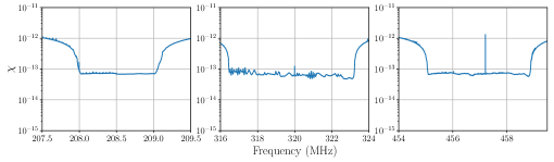
Figure 18: Exclusion limits for the kinetic mixing of hidden photons obtained from the resonant signal scans of WISPDMX measurements at a 95% confidence level.

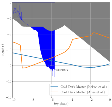
Figure 19: The combined 95% exclusion limits for the hidden photon kinetic mixing obtained from the resonant and broadband signal scans of the WISPDMX measurements. The gray shade denotes cumulative exclusion limits obtained in previous experiments [33, 34, 35, 36].

Figure 19 shows that the WISPDMX measurements have improved the existing exclusion limits in a broad range of hidden photon mass, from $0.4\text{\,}\mathrm{neV}$ to $2.07\text{\,}\mathrm{\SIUnitSymbolMicro eV}$. Above $\approx 0.1$\mathrm{\SIUnitSymbolMicro eV}$$, the WISPDMX has excluded part of the parameter space for the hidden photon dark matter predicted in the misalignment Skotinogenesis scenarios [5, 6].

6 Discussion

The measurements described in this paper comprise the first fully automated science run made with the WISPDMX apparatus, achieving a substantial improvement in comparison to the earlier trial runs made in the untuned [37, 38] and partially tuned [39] modes of operation. The present measurements extend the existing haloscope exclusion limits for hidden photon dark matter (calculated in [6] using the results from several axion dark matter searches [11, 40, 41]) to masses below $2.07\text{\,}\mathrm{\SIUnitSymbolMicro eV}$ and pioneer a combination of resonant and broadband signal search, extending the search range down to $0.4\text{\,}\mathrm{neV}$.

For the resonant modes, the sensitivity and exclusion limits can potentially be improved by applying the multiple bin analysis used in [42]. The quality of the broadband spectrum can be improved if the measurements are repeated in a better shielded environment which should help reducing the interference from external radio frequency signals, especially within the FM radio band at $80\text{\,}\mathrm{MHz}110\text{\,}\mathrm{MHz}$.

A dedicated multiple-run arrangement in which measurements at each given cavity tuning performed at three different local sidereal times would further refine the results by improving the experiment sensitivity to local dark matter flows with non-isotropic directional distribution of the particle velocity [6]. With the cavity positioned at a 45^∘ angle with respect to the rotational axis of the Earth, one of these three measurements should fall with a factor of 0.75 of the sensitivity expected for the isotropic directional distribution.

The nature of the signal candidate found at $218.017\,395\text{\,}\mathrm{MHz}$ ($0.901\,647\,83\text{\,}\mathrm{\SIUnitSymbolMicro eV}$) needs to be better understood. The halo velocity dispersion of $330\text{\,}\mathrm{k}\mathrm{i}\mathrm{l}\mathrm{o}\mathrm{m}\,\mathrm{s}^{-1}$ inferred from this signal agrees well with the observational estimates [21, 22]. The total excess power of $(1.8\pm 0.2)\times 10^{-21}$\mathrm{W}$$ measured in the fitted profile can be reconciled with the estimated energy density of the Galactic dark matter halo composed of hidden photons kinetically mixed with normal photons at $\chi=(1.1\,^{+0.6}_{-0.2})\times 10^{-12}$. Thus the shape, the width, and the strength of this signal candidate can reconcile it with the signal from the hidden photon dark matter [5, 6]. However, the physical relevance of this signal still needs to be investigated further, particularly with respect to its potential relation to a periodic interference signal identified throughout a broader frequency range in the measured spectrum.

Such an investigation will be realized by repeating the WISPDMX runs with a better shielding, an improved apparatus, and at different times of the year. The first two measures would provide a better account of potential instrumental effects, while the latter one should constrain the physical relevance of the signal by looking for its expected annual modulation. With the parameters of the tentative signal, the expected frequency shift of the signal due to the annual modulation should be $\approx 16.0$\mathrm{Hz}$$, which can be detected already at the present frequency resolution of $50\text{\,}\mathrm{Hz}$ and the signal strength ($\mathrm{SNR}\approx 10$).

The overall results obtained with the WISPDMX so far demonstrate the potential of employing a haloscope setup to unveil the nature of hidden photon dark matter by combining signal detection at multiple resonant mode and non-resonant detection over a broad range of frequency. Such a combination has become possible due to implementation of a high resolution, broadband recording setup which provides a frequency resolution of $50\text{\,}\mathrm{Hz}$ over a $500\text{\,}\mathrm{MHz}$ bandwidth.

The high-efficiency acquisition system of WISPDMX provides a methodological foundation for future broadband experiments aimed at searching for either the hidden photon or the axion dark matter. The WISPDMX measurements also pave the way to generic heterodyne experiments at the particle masses below $1\text{\,}\mathrm{\SIUnitSymbolMicro eV}$, where both resonant [43, 44] and inherently broadband setups can be employed.

References

- [1] M. Dine, Naturalness Under Stress, Ann. Rev. Nucl. Particle Sci. 65 (2015) 43.
- [2] D. Scott, The Standard Model of Cosmology: A Skeptic’s Guide, arXiv:1804.01318 [astro-ph] (2018) .
- [3] L. B. Okun, The limits of electrodynamics - Paraphotons, ZhETF 83 (1982) 892.
- [4] M. Goodsell, J. Jaeckel, J. Redondo and A. Ringwald, Naturally Light Hidden Photons in LARGE Volume String Compactifications, JHEP 0911 (2009) 027.
- [5] A. E. Nelson and J. Scholtz, Dark light, dark matter, and the misalignment mechanism, Phys. Rev. D 84 (2011) 103501.
- [6] P. Arias, D. Cadamuro, M. Goodsell, J. Jaeckel, J. Redondo and A. Ringwald, WISPy cold dark matter, JCAP 06 (2012) 013.
- [7] P. W. Graham, J. Mardon and S. Rajendran, Vector dark matter from inflationary fluctuations, Phys. Rev. D 93 (2016) 103520 [1504.02102].
- [8] B. Holdom, Two U(1)’s and charge shifts, Phys. Lett. B 166 (1986) 196.
- [9] S. A. Abel, M. D. Goodsell, J. Jaeckel, V. V. Khoze and A. Ringwald, Kinetic Mixing of the Photon with Hidden U(1)s in String Phenomenology, JHEP 2008 (2008) 124.
- [10] R. Essig, J. A. Jaros, W. Wester, P. Hansson Adrian, S. Andreas, T. Averett et al., Dark Sectors and New, Light, Weakly-Coupled Particles, ArXiv e-prints 1311 (2013) arXiv:1311.0029.
- [11] R. Bradley, J. Clarke, D. Kinion, L. J. Rosenberg, K. van Bibber, S. Matsuki et al., Microwave cavity searches for dark-matter axions, Reviews of Modern Physics 75 (2003) 777.
- [12] P. Sikivie, Experimental Tests of the "Invisible" Axion, Phys. Rev. Lett. 51 (1983) 1415.
- [13] P. Arias, A. Arza, B. Döbrich, J. Gamboa and F. Méndez, Extracting hidden-photon dark matter from an LC-circuit, European Physical Journal C 75 (2015) 310 [1411.4986].
- [14] J. A. R. Cembranos, C. Hallabrin, A. L. Maroto and S. J. N. Jareño, Isotropy theorem for cosmological vector fields, Phys. Rev. D 86 (2012) 021301 [1203.6221].
- [15] N. W. Evans, C. A. J. O’Hare and C. McCabe, Refinement of the standard halo model for dark matter searches in light of the Gaia Sausage, Phys. Rev. D 99 (2019) 023012.
- [16] L. D. Duffy and P. Sikivie, Caustic ring model of the MilkyWay halo, Phys. Rev. D 78 (2008) 063508 [0805.4556].
- [17] M. Vogelsberger and S. D. M. White, Streams and caustics: the fine-grained structure of cold dark matter haloes, MNRAS 413 (2011) 1419 [1002.3162].
- [18] E. W. Lentz, T. R. Quinn, L. J. Rosenberg and M. J. Tremmel, A New Signal Model for Axion Cavity Searches from N-body Simulations, Astrophys. J. 845 (2017) 121 [1703.06937].
- [19] J. I. Read, The local dark matter density, J. Phys. G: Nucl. and Part. Phys. 41 (2014) 063101.
- [20] M. S. Turner, Periodic signatures for the detection of cosmic axions, Pys. Rev. D 42 (1990) 3572.
- [21] A. M. Green, Astrophysical uncertainties on direct detection experiments, Mod. Phys. Lett. A27 (2012) 1230004 [1112.0524].
- [22] F. J. Kerr and D. Lynden-Bell, Review of galactic constants, Monthly Notices of the Royal Astronomical Society 221 (1986) 1023.
- [23] C. A. J. O’Hare and A. M. Green, Axion astronomy with microwave cavity experiments, Phys. Rev. D 95 (2017) 063017 [1701.03118].
- [24] K. Griest, Effect of the Sun’s gravity on the distribution and detection of dark matter near the Earth, Phys. Rev. D 37 (1988) 2703.
- [25] T. Marrodán Undagoitia and L. Rauch, Dark matter direct-detection experiments, J. Phys. G43 (2016) 013001 [1509.08767].
- [26] M. C. Smith et al., The RAVE Survey: Constraining the Local Galactic Escape Speed, Mon. Not. Roy. Astron. Soc. 379 (2007) 755 [astro-ph/0611671].
- [27] A. Pillepich, M. Kuhlen, J. Guedes and P. Madau, The Distribution of Dark Matter in the Milky Way’s Disk, Astrophys. J. 784 (2014) 161 [1308.1703].
- [28] A. J. Deason, A. Fattahi, V. Belokurov, N. W. Evans, R. J. J. Grand, F. Marinacci et al., The local high-velocity tail and the Galactic escape speed, Mon. Not. Roy. Astron. Soc. 485 (2019) 3514 [1901.02016].
- [29] A. Gamp, The Radio Frequency Systems And Control Of The HERA Proton Beam, Part. Accel. 29 (1990) 65.
- [30] G. Rogner, Study of the mechanical design of 200 MHz single-cell cavities for application in the SPS. CERN, Geneva, 1980.
- [31] V. Rödel, Higher-order modes and tuning of the SPS 200 MHz single-cell cavity, Tech. Rep. CERN-SL-RFS-Note-91-08. SL-RFS-Note-91-08, CERN, Geneva, Nov, 1991.
- [32] “CST — Computer Simulation Technology.” www.CST.com, 2015-2016.
- [33] D. J. Fixsen, E. S. Cheng, J. M. Gales, J. C. Mather, R. A. Shafer and E. L. Wright, The Cosmic Microwave Background Spectrum from the Full COBE FIRAS Data Set, APJ 473 (1996) 576 [astro-ph/9605054].
- [34] H. Georgi, P. H. Ginsparg and S. L. Glashow, Photon Oscillations and the Cosmic Background Radiation, Nature 306 (1983) 765.
- [35] A. Mirizzi, J. Redondo and G. Sigl, Microwave Background Constraints on Mixing of Photons with Hidden Photons, JCAP 0903 (2009) 026 [0901.0014].
- [36] S. G. Karshenboim, Precision physics of simple atoms and constraints on a light boson with ultraweak coupling, Phys. Rev. Lett. 104 (2010) 220406 [1005.4859].
- [37] S. Baum, WISPDMX - Eine direkte Suche nach Dunkler Materie mit einer 208 MHz HERA-Kavität, B.S. Thesis, Universität Hamburg, 2013. 2013-12-04.
- [38] D. Horns, A. Lindner, A. P. Lobanov and A. Ringwald, WISP Dark Matter eXperiment and Prospects for Broadband Dark Matter Searches in the eV–meV Mass Range, in Proc. of 10th Patras Workshop on Axions, WISPs, and WISPs, pp. 1–8, Oct., 2014, 1410.6302.
- [39] L. H. Nguyen, D. Horns, A. P. Lobanov and A. Ringwald, WISPDMX: A haloscope for WISP Dark Matter between 0.8-2 eV, in Proc. of 11th Patras Workshop on Axions, WISPs, and WISPs, pp. 1–6, Nov., 2015, 1511.03161.
- [40] S. J. Asztalos, R. F. Bradley, L. Duffy, C. Hagmann, D. Kinion, D. M. Moltz et al., Improved rf cavity search for halo axions, Phys. Rev. D 69 (2004) 011101 [astro-ph/0310042].
- [41] S. J. Asztalos, G. Carosi, C. Hagmann, D. Kinion, K. van Bibber, M. Hotz et al., SQUID-Based Microwave Cavity Search for Dark-Matter Axions, Phys. Rev. Lett. 104 (2010) 041301 [0910.5914].
- [42] S. Asztalos, E. Daw, H. Peng, L. J. Rosenberg, C. Hagmann, D. Kinion et al., Large-scale microwave cavity search for dark-matter axions, Phys. Rev. D 64 (2001) 092003.
- [43] S. Chaudhuri, P. W. Graham, K. Irwin, J. Mardon, S. Rajendran and Y. Zhao, Radio for hidden-photon dark matter detection, Phys. Rev. D 92 (2015) 075012 [1411.7382].
- [44] S. Chaudhuri, K. Irwin, P. W. Graham and J. Mardon, Fundamental Limits of Electromagnetic Axion and Hidden-Photon Dark Matter Searches: Part I - The Quantum Limit, arXiv e-prints (2018) [1803.01627].