New physics from COHERENT data with improved Quenching Factor

Abstract

A recent new measurement and re-analysis of past measurements suggested an improved quenching factor value and uncertainty for CsI[Na]. This implies a measurement of the COHERENT experiment of coherent elastic neutrino-nucleus scattering that is closer to the Standard Model prediction and has less uncertainty. We illustrate the impact of this improvement by revisiting fits to the Weinberg angle, neutrino magnetic moments, neutron rms and neutrino charge radii, weak nuclear charge of the Cs nucleus, neutrino non-standard interactions (in particular those relevant for LMA-Dark) and new scalar as well as vector bosons. Significant improvement is observed, particularly for those scenarios coherently affecting the electroweak SM process.

I Introduction

Coherent elastic neutrino-nucleus scattering (CE$\nu$NS) has been predicted in 1974 Freedman (1974), but not been observed before 2017 Akimov et al. (2017). The importance of the process ranges from its ability to probe Standard Model parameters at low momentum transfer Scholberg (2006); Lindner et al. (2017); Miranda et al. (2019a), test new neutrino physics and new neutral currents in general Barranco et al. (2005); Dutta et al. (2016a); Lindner et al. (2017); Dent et al. (2017); Coloma et al. (2017); Liao and Marfatia (2017); Dent et al. (2018); Papoulias and Kosmas (2018); Farzan et al. (2018); Abdullah et al. (2018); Bauer et al. (2018); Heeck et al. (2019); Denton et al. (2018); Billard et al. (2018); Altmannshofer et al. (2018); Aristizabal Sierra et al. (2019a); Miranda et al. (2019b); Dutta et al. (2019a); Aristizabal Sierra et al. (2019b); Bischer and Rodejohann (2019); Arcadi et al. (2019), sterile neutrino searches Anderson et al. (2012); Dutta et al. (2016b); Papoulias and Kosmas (2018); Aristizabal Sierra et al. (2019a); Miranda et al. (2019b), implications for supernova physics Freedman et al. (1977); Melson and Janka (2019); Raj et al. (2019); Raj (2019), dark matter searches deNiverville et al. (2015); Ge and Shoemaker (2018); Brdar et al. (2018); Dutta et al. (2019b); Chao et al. (2019), neutrino magnetic moments Dodd et al. (1991); Scholberg (2006); Kosmas et al. (2015); Papoulias and Kosmas (2018); Billard et al. (2018); Miranda et al. (2019a), nuclear physics Cadeddu et al. (2018a); Huang and Chen (2019); Papoulias et al. (2019); Ciuffoli et al. (2018) and its connection to gravitational waves Hagen et al. (2015); Wei et al. (2019). The process under discussion is taking place at energies below about 50 MeV, and given by

$$\nu+N\to\nu+N\,.$$ (1)

Nuclear recoil is the relevant observable. In case of COHERENT, a CsI[Na] scintillation detector was used as target. Experimentally, the so-called Quenching Factor (QF) is of crucial importance. It denotes the energy-dependent ratio of the scintillation signal from nuclear recoils with respect to the one from electron recoils, i.e. the ratio of recorded energy to nuclear recoil. In the publication of the COHERENT experiment the QF-uncertainty of 18.9% dominated the total uncertainty Akimov et al. (2017). Recently, past measurements of the QF were revisited, and a new one was performed Collar et al. (2019). As a result, new (energy-dependent) values for the QF and its uncertainty were proposed. Applied to COHERENT, the systematic uncertainty would reduce from 28% to 13.5%, and the SM-predicted rate would reduce from $173\pm 48$ to $138\pm 19$, compared to the measurement of $134\pm 22$ events. As suggested in Collar et al. (2019), physics extracted from the measurement would significantly improve when taking into account the new QF-values and uncertainty.

We perform in this paper, as illustration of the impact of improved quenching understanding, a fit to COHERENT data taking into account the new QF value and uncertainty. We consider several parameters that can be extracted from CE$\nu$NS, namely the Weinberg angle, neutrino magnetic moment and charge radii, the neutron rms charge radius, neutrino non-standard interactions, as well as couplings and masses of new vector and scalar bosons mediating CE$\nu$NS. Improvement is found, particularly for those scenarios that coherently affect the SM process.

The paper is built up as follows. In Section II we describe the data we fit and the procedure we follow. Section III gives the fit results for parameters related to SM and new electroweak physics, namely the Weinberg angle, neutrino magnetic moments and neutron/neutrino charge radii. Section IV deals with neutrino non-standard interactions, Section V with parameters related to new vector or scalar bosons, before we conclude in Section VI.

II COHERENT Data and Fit Procedure

The neutrino source for COHERENT’s detection of coherent elastic neutrino-nucleus scattering are pions produced from the spallation neutron source. The total number of protons on target (POT) delivered to a liquid mercury target was $N_{\mathrm{POT}}^{\rm tot}=1.76\times 10^{23}$ Akimov et al. (2017). Monoenergetic muon neutrinos $(\nu_{\mu})$ at $E_{\nu}=29.9$ MeV are produced from pion decay at rest ($\pi^{+}\rightarrow\mu^{+}\nu_{\mu})$, followed by a delayed beam of electron neutrinos ($\nu_{e})$ and muon-antineutrinos ($\bar{\nu}_{\mu})$ produced subsequently by muon decay $\mu^{+}\rightarrow\nu_{e}\,e^{+}\bar{\nu}_{\mu}$. The average production rate from the pion decay chain is $r=0.08$ neutrinos of each flavor per proton.

The CsI[Na] scintillator detector is located at a distance of $L=19.3$ m. The fluxes are Akimov et al. (2018)

$$\frac{d\phi_{\nu_{\mu}}(E_{\nu})}{dE_{\nu}} = \frac{rN_{pot}}{4\pi L^{2}}\delta\left(E_{\nu}-\frac{m_{\pi}^{2}-m_{\mu}^{2}}{2m_{\pi}}\right),$$

$$\frac{d\phi_{\overline{\nu}_{\mu}}(E_{\nu})}{dE_{\nu}} = \frac{rN_{pot}}{4\pi L^{2}}\frac{64E_{\nu}^{2}}{m_{\mu}^{3}}\left(E_{\nu}-\frac{m_{\pi}^{2}-m_{\mu}^{2}}{2m_{\pi}}\right),$$

$$\frac{d\phi_{\nu_{e}}(E_{\nu})}{dE_{\nu}} = \frac{rN_{pot}}{4\pi L^{2}}\frac{192E_{\nu}^{2}}{m_{\mu}^{3}}\left(\frac{1}{2}-\frac{E_{\nu}}{m_{\mu}}\right),$$ (2)

where $N_{pot}=5.71\times 10^{20}$ are the number of protons per day. The differential cross section of CE$\nu$NS with respect to the nuclear recoil energy $T$, for neutrinos with energy $E_{\nu}$ scattered off a target nucleus $(A,Z)$, can be written as

$$\frac{d\sigma}{dT}(E_{\nu},T)\simeq\frac{G_{F}^{2}M}{\pi}Q_{W}^{2}\left(1-\frac{MT}{2E_{\nu}^{2}}\right)F^{2}(q^{2})\,,$$ (3)

where $G_{F}$ is the Fermi constant, $M$ the nuclear mass, $T$ is nuclear recoil energy, and $Q_{W}^{2}$ is the weak nuclear charge

$$Q_{W}^{2}=\left[Zg_{p}^{V}+Ng_{n}^{V}\,\right]^{2}\,.$$ (4)

Here $Z$ is the proton number, $N$ the neutron number (tiny contributions from the sodium dopant of the detector can be ignored Akimov et al. (2018)), and the standard vector coupling constants are $g_{p}^{V}=1/2-2\sin^{2}\theta_{W}$, $g_{n}^{V}=-1/2$. Finally, $F(q^{2})$ is the nuclear form factor, we use the Klein-Nystrand parametrisation Klein and Nystrand (1999); Engel (1991):

$$F(q^{2})=\frac{4\pi\rho_{0}}{Aq^{3}}[\sin(qR_{A})-qR_{A}\cos(qR_{A})]\left[\frac{1}{1+a^{2}q^{2}}\right].$$ (5)

Here $q^{2}=2MT$ is the momentum transfer in the scattering of neutrinos off the CsI nuclei, $\rho_{0}$ is the normalized nuclear density, $R_{A}=1.2A^{1/3}\,\mathrm{fm}$ is the nuclear radius and $a=0.7\,\mathrm{fm}$ is the range of the Yukawa potential. Following Ref. Akimov et al. (2017) we will treat form factors entering the Cs and I cross-sections as the same.

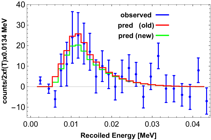
Figure 1: The SM expected nuclear recoil energy spectrum of CE$\nu$NS for the COHERENT setup as function of the recoil energy. The points with the vertical error bars correspond to the COHERENT data. The expected spectrum was obtained with the new quenching factor. The old spectrum (red) has been re-scaled horizontally for comparison with the new result (green).

The differential event rate, after taking into account the detection efficiency $\epsilon(T)$, taken from Fig. S9 in Ref. Akimov et al. (2017), of COHERENT reads

$$\frac{dN_{\nu_{\alpha}}}{dT}=tN\underset{E_{\nu}^{\min}}{\int\limits^{E_{\nu}^{\max}}}dE_{\nu}\frac{d\sigma}{dT}(E_{\nu},T)\frac{d\phi_{\nu_{\alpha}}(E_{\nu})}{dE_{\nu}}\epsilon(T)\,,$$ (6)

where $t=308.1$ days is the run time of the experiment, $N=\frac{2m_{\mathrm{det}}}{M_{\rm CsI}}N_{A}$ is the total number of target nucleons, $m_{\mathrm{det}}=14.57$ kg, $N_{A}$ is Avogadro’s number and $M_{\rm CsI}$ is the molar mass of CsI.

In the first result of COHERENT Akimov et al. (2017) the expected number of photo-electrons (p.e.) was 0.00117 p.e. ($T\!/\rm MeV$). The recent new measurement from Ref. Collar et al. (2019) improves this value and moreover gives its energy dependence. We can use the following relation between the recoil energy and number of photo-electrons:

$$N(p.e.)=f(T)\times 0.0134\ (T\!/{\rm MeV})\,,$$

where $f(T)$ is the new quenching factor whose energy dependence is given in the left panel of Fig. 1 in Ref.  Collar et al. (2019). For the acceptance function, we use Eq. (1) of Ref. Akimov et al. (2018) as recommended there:

$$\epsilon(T)=\frac{a_{1}}{1+\exp(-a_{2}(T-T_{0}))}\Theta(T)\,.$$ (7)

Here $a_{1}=0.6655$, $a_{2}=494.2$ MeV^-1, $T_{0}=0.0092741$ MeV and the Heaviside function reads

$$\Theta(x)=\left\{\begin{array}[]{c}0\ \ \ \ \ \ \ \ \ \ \ \ x<5,\\ 0.5\ \ \ \ 5\leq x<5,\\ 1\ \ \ \ \ \ \ \ \ \ \ \ \ \ \ x\geq 6.\end{array}\right.$$

All results in this paper will be derived by considering the following $\chi^{2}$-function:

$$\chi^{2}=\underset{i=4}{\overset{20}{\sum}}\frac{[N_{obs}^{i}-N_{exp}^{i}(1+\alpha)-B^{i}(1+\beta)]^{2}}{(\sigma^{i})^{2}}+\left(\frac{\alpha}{\sigma_{\alpha}}\right)^{2}+\left(\frac{\beta}{\sigma_{\beta}}\right)^{2}\,.$$ (8)

Here $N_{obs}^{i}$ is the observed event rate in the $i$-th energy bin, $N_{exp}^{i}$ is the expected event rate given in Eq. (6) integrated over the recoiled energy corresponding to each flavor, and $B^{i}$ is the estimated background event number in the $i$-th energy bin extracted from Fig. S13 of Ref.  Akimov et al. (2017). The statistical uncertainty in the $i$-th energy bin is $\sigma^{i}$, and $\alpha$, $\beta$ are the pull parameters related to the signal systematic uncertainty and the background rates. The corresponding uncertainties of the pull parameters are $\sigma_{\alpha}=0.28$ (previous value Akimov et al. (2017)) $0.135$ (new value Collar et al. (2019)) and $\sigma_{\beta}=0.25$. We calculate $\sigma_{\alpha}$ by adding the flux uncertainty (10%), neutron capture (5%), acceptance (5%), QF (25%-old and 5.1%-new) in quadrature. The effect of the new quenching factor with the improved uncertainty on the recoiled energy spectrum is shown in Fig. 1 in red (old) and green (new).

Note that for simplicity we do not fit the prompt $\nu_{\mu}$ and the delayed $\nu_{e}$, $\bar{\nu}_{\mu}$ separately. In the plots that will be presented in what follows, our best-fit value is always indicated by a black dot. The total event rate we obtained with the above set by summing over all the energy bins are  167 (previous) and  139 (new) which are well within 1 sigma of the expected values of $173\pm 48$ (old) and $138\pm 19$ (new), respectively.

III Constraints on electroweak physics of neutrinos

In this section discuss the improved constraints on the Weinberg angle $\sin^{2}\theta_{W}$, on parameters related to possible new electromagnetic properties of neutrinos, and on the neutron rms charge radius.

III.1 Evaluation of $\sin^{2}\theta_{W}$

Since the systematic effects are directly correlated with the electroweak physics parameters of CE$\nu$NS, any improvement in the quenching factor significantly affects for $\sin^{2}\theta_{W}$ its best-fit value and uncertainty. The dependence on the Weinberg angle enters via $g_{n}^{V}$ in Eq. (4) in the differential cross section Eq.  (3). The $\Delta\chi^{2}$-distributions of $\sin^{2}\theta_{W}$ with old and new systematic uncertainties are displayed in the upper left plot of Fig. 2. It is evident from the figure that the central value of $\sin^{2}\theta_{W}$ has significantly shifted towards a larger value. The new value from the COHERENT data with improved systematics is now

$$\sin^{2}\theta_{W}=0.248\pm 0.045\,(1\sigma)\pm 0.074\,(90\%\,{\rm C.L.}),$$ (9)

whereas the older value with 28% systematic uncertainty is $\sin^{2}\theta_{W}=0.217_{-0.051}^{+0.068}\,(1\sigma)_{-0.08}^{+0.13}\,(90\%\ {\rm C.L.})$. The prediction of the modified $\overline{MS}$ renormalization scheme for sub-MeV momentum regime at low energy is $\sin^{2}\theta_{W}=0.23867\pm 0.00016$ Erler and Ramsey-Musolf (2005) at 90% C.L. The fact that COHERENT data with the original QF yields a value smaller than the SM prediction is consistent with Refs.  Papoulias and Kosmas (2018); Huang and Chen (2019); Cadeddu and Dordei (2019). The new fit-result has an about 20% smaller error and is closer to the SM-prediction. The error is also much more Gaussian.

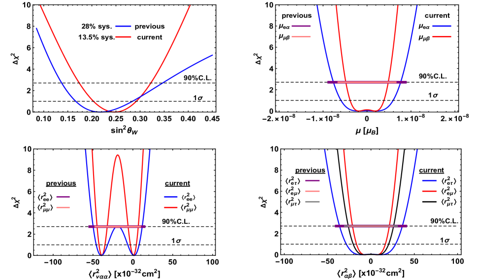
Figure 2: 1-dimensional $\Delta\chi^{2}$-distributions of $\sin^{2}\theta_{W}$ (top-left), neutrino magnetic moments (top-right) and charge radii (lower left+right). For $\sin^{2}\theta_{W}$ results with previous and current QF values are shown by separate curves, while for all other cases the previous results are shown through horizontal lines at 90% C.L.

III.2 Neutrino magnetic moments

Magnetic moments appear in the general coupling of neutrinos to the electromagnetic field strength for Majorana ($M$) or Dirac ($D$) neutrinos

$${\cal L}^{M}=-\frac{1}{4}\bar{\nu}_{\alpha L}^{c}\,\lambda_{\alpha\beta}^{M}\,\sigma_{\mu\nu}\,\nu_{\beta L}\,F^{\mu\nu}~{}\mbox{ or }~{}{\cal L}^{D}=-\frac{1}{2}\bar{\nu}_{\alpha R}\,\lambda_{\alpha\beta}^{D}\,\sigma_{\mu\nu}\,\nu_{\beta L}\,F^{\mu\nu}\,.$$ (10)

Here $\lambda^{X}=\mu^{X}-i\epsilon^{X}$, which is antisymmetric (hermitian) for Majorana (Dirac) neutrinos. Complex phases and $\epsilon^{X}$ are ignored here, see Ref. Miranda et al. (2019a) for a general discussion. For Majorana neutrinos, in particular, there are only transition magnetic moments, $\mu^{M}_{\alpha\alpha}=0$. With unknown final state neutrino flavor no distinction between Dirac and Majorana neutrinos is possible. We assume here for definiteness Majorana neutrinos (and will drop the superscript $M$ from now on) and thus are sensitive to $\mu_{e\alpha}$ and $\mu_{\mu\beta}$ with $\alpha=\mu,\tau$ and $\beta=e,\tau$.

The contribution of a helicity-changing neutrino magnetic moment contribution adds to the helicity-conserving SM cross-section incoherently. Therefore we can make for the case of $\nu_{e}$ the replacement $Q_{W}^{2}\rightarrow Q_{W}^{2}+Q_{mm,e}^{2}$, where $Q_{W}^{2}$ is given in Eq. (4) and

$$Q_{mm,e}^{2}=\left(\frac{\pi\alpha_{em}\,\mu_{e\alpha}\,Z}{2\sqrt{2}G_{F}m_{e}}\right)^{2}\text{ }\left(\frac{1}{T}-\frac{1}{E_{\nu}}+\frac{T}{4E_{\nu}^{2}}\right)\frac{8}{M\left(1-\frac{MT}{2E_{\nu}^{2}}\right)}$$ (11)

and analogously for $\nu_{\mu}$/$\bar{\nu}_{\mu}$. Here $\alpha_{em}$ is the fine-structure constant, $m_{e}$ the electron mass and $\mu_{e\alpha}$ is the effective neutrino magnetic moment in units of Bohr magnetons $\mu_{B}$. The result of the fits is shown in Fig.  2 (top-right) for one parameter at-a-time and in Fig. 3 for two-parameter fitting. In the 1-dimensional plot, the previous constraints are shown for comparison at 90% C.L. for each case. Improvement can be clearly seen for both parameters. The new constraints obtained from one parameter at-a-time fitting at 90% C.L. in units of $\mu_{B}$ are

$$-76\times 10^{-10} < \mu_{e\alpha}/\mu_{B}<76\times 10^{-10}\,,$$ (12)

$$-48\times 10^{-10} < \mu_{\mu\beta}/\mu_{B}<48\times 10^{-10}\,,$$ (13)

while the previous constraints from our analysis are $-86\times 10^{-10}<\mu_{e\alpha}/\mu_{B}<86\times 10^{-10}$ and $-57\times 10^{-10}<\mu_{\mu\beta}/\mu_{B}<57\times 10^{-10}$, respectively. Improvement by 13% and 20% is found for $\mu_{e\alpha}$ and $\mu_{\mu\beta}$ when an improved QF is taken into account.

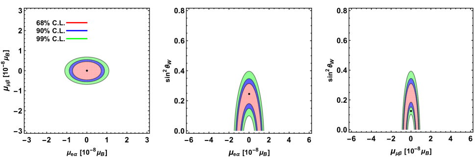
Figure 3: 2-dimensional $\Delta\chi^{2}$-contour plots for various combinations of $\sin^{2}\theta_{W}$ and magnetic moments with 68%, 90% and 99% C.L. boundaries.

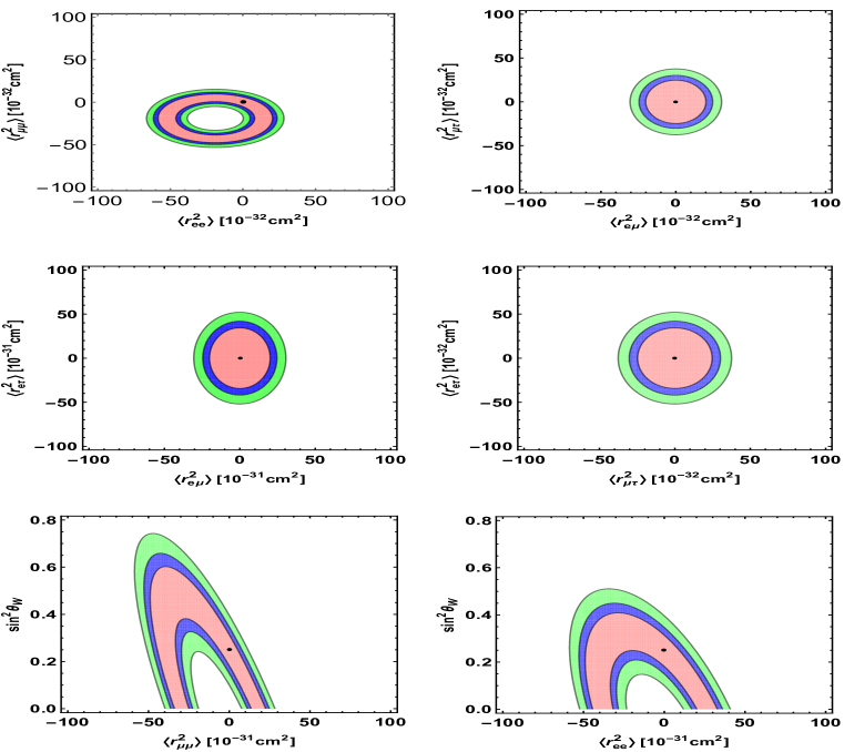
Figure 4: 2-dimensional $\Delta\chi^{2}$-contour plots for various combinations of $\sin^{2}\theta_{W}$ and neutrino charge radii with 68%, 90% and 99% C.L.  boundaries.

III.3 Neutrino charge radii

Massive neutrinos have an effective electromagnetic vertex $\bar{\nu}\Lambda_{\mu}\nu A^{\mu}$ with Giunti and Studenikin (2015); Cadeddu et al. (2018b)

$$\Lambda_{\mu}(q)=\gamma_{\mu}F(q^{2})\simeq\gamma_{\mu}q^{2}\frac{\langle r^{2}\rangle}{6}\,,$$

where $q$ is the momentum transfer and $F(q^{2})$ is a form factor connected to the neutrino charge radius $\langle r^{2}\rangle$ via

$$\langle r^{2}\rangle=6\left.\frac{dF_{\nu}(q^{2})}{dq^{2}}\right|_{q^{2}=0}\,.$$

The expression in the SM Bernabeu et al. (2000, 2002, 2004) is

$$\langle r_{\alpha\alpha}^{2}\rangle_{\rm SM}=-\frac{G_{F}}{2\sqrt{2}\pi}\left[3-2\ln\left(\frac{m_{\alpha}^{2}}{m_{W}^{2}}\right)\right],$$

where $m_{\alpha}$ is the mass of the charged lepton associated to $\nu_{\alpha}$. Only diagonal charge radii $\langle r_{\alpha\alpha}^{2}\rangle$ exist in the SM, while in general also transition charge radii $\langle r_{\alpha\beta}^{2}\rangle$ are possible. The former add coherently to the SM process, and we can take their effect into account by making for incoming neutrinos of flavor $\alpha$ the replacement $g_{p}^{V}\rightarrow g_{p}^{V}+g_{em,\alpha}^{V},$ where $g_{p}^{V}$ is given above Eq. (4) and

$$g_{em,\alpha}^{V}=-\frac{\sqrt{2}\pi\alpha_{em}}{3G_{F}}\text{ }\langle r_{\alpha\alpha}^{2}\rangle\,.$$ (14)

For the COHERENT setup, $\langle r_{ee}^{2}\rangle$ and $\langle r_{\mu\mu}^{2}\rangle$ are relevant. The contribution of the flavor transition charge radii adds incoherently to the flavor-conserving SM process. Hence we can make for $\nu_{e}$ the replacement $Q_{W}^{2}\rightarrow Q_{W}^{2}+Q_{em,e}^{2}$, where $Q_{em,e}^{2}$ is given by

$$Q_{em,e}^{2}=\left(\frac{\sqrt{2}6\pi\alpha_{em}Z}{3G_{F}}\text{ }\langle r_{e\alpha}^{2}\rangle\right)^{2}\,$$ (15)

where $\alpha=\mu,\tau$. While the neutrino flux at COHERENT includes $\nu_{\mu}$ and $\overline{\nu}_{\mu}$, since the transition charge radii of anti-neutrinos change only sign with respect to the ones for neutrinos Giunti and Studenikin (2015), only three flavor transition charge radii parameters are present: $\langle r_{e\mu}^{2}\rangle,\ \langle r_{e\tau}^{2}\rangle$ and $\langle r_{\mu\tau}^{2}\rangle$. However, we have realized that this in principle is correct, but since the the weak neutral current couplings also change their signs from neutrinos to anti neutrinos under CP-transformation which leaves the overall sign of the term $g_{p}^{V}+g_{em,\alpha}^{V},$ unchanged. As a result, the sign changing for the neutrino charge radii for muon anti-neutrino has no effects and we get similar $\chi^{2}$-distribution of $\langle r_{\mu\mu}^{2}\rangle$ and $\langle r_{\mathrm{e}\mathrm{e}}^{2}\rangle$ as shown in the lower left panel in fig. 2.

The results for one parameter at-a-time and two parameter fitting are shown in Figs. 2 (lower 2 panels) and 4, respectively. In Fig. 2, the results for 28% systematic errors are shown using horizontal lines at 90% C.L. for comparison. Improvement by (13-40)% is found when an improved QF is taken into account. Our 90% C.L. constraints on the neutrino charge radii, in units of cm², are

$$-48\times 10^{-32} < \langle r_{ee}^{2}\rangle/{\rm cm^{2}}<12\times 10^{-32}\,,$$

$$-44\times 10^{-32} < \langle r_{\mu\mu}^{2}\rangle/{\rm cm^{2}}<6\times 10^{-32}\,,$$

$$-8\times 10^{-32} < \langle r_{e\mu}^{2}\rangle/{\rm cm^{2}}<8\times 10^{-32}\,,$$ (16)

$$-18\times 10^{-32} < \langle r_{e\tau}^{2}\rangle/{\rm cm^{2}}<18\times 10^{-32}\,,$$

$$-12\times 10^{-32} < \langle r_{\mu\tau}^{2}\rangle/{\rm cm^{2}}<12\times 10^{-32}\,.$$

III.4 Neutron Charge Radius and Cs weak nuclear charge

Nuclear physics parameters can be tested by coherent scattering as well. We estimate here the neutron charge radius of CsI nuclei using the improved QF following the prescription of Ref.  Cadeddu et al. (2018a). We use the form factor defined in Eq. (5) both for protons and neutrons except that for neutrons we replace $R_{A}$ by

$$R_{A}=\sqrt{\frac{5}{3}(R_{n}^{2}-6a^{2})}\,,$$

Here $R_{n}$ is the root-mean-square (rms) neutron charge radius. Notice that all results are obtained in the approximation that the radii are the same for Cs and I.

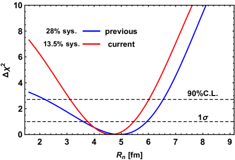
Figure 5: 1-dim $\Delta\chi^{2}$ for the neutron rms charge radius.

We obtain the following best-fit values of the neutron charge radius of ¹³³Cs and ¹²⁷I

$$R_{n} = 4.6_{-0.8}^{+0.9}\ {\rm fm}\ (1\sigma)\ \ \ (\text{current}),$$ (17)

$$R_{n} = 4.9_{-1.3}^{+1.1}\ {\rm fm}\ (1\sigma)\ \ \ (\text{previous}).$$ (18)

The $\Delta\chi^{2}$-distribution of a one-parameter fit is shown in Fig. 5. Notice that with the improved QF, there is 10% improvement in uncertainty, the distribution becomes more Gaussian, and the best-fit value is shifted towards a relatively lower value. Notice that the value obtained in Ref.  Cadeddu et al. (2018a) was $R_{n}=5.5_{-1.1}^{+0.9}\ {\rm fm}$, which is consistent within $1\sigma$.

We note at this point that Ref. Cadeddu et al. (2019) appeared a few days after this work, and that in particular the best-fit point of $R_{n}$ differs considerably. We find that this can be traced mainly to our use of 17 energy bins and the Klein-Nystrand form factor, compared to 12 bins and the Helm form factor in Ref. Cadeddu et al. (2019). Indeed, repeating our fit with 12 energy bins and the Helm form factor yields a best-fit value of $R_{n}=4.9$ fm, compared to the value $R_{n}=5.0$ fm in Ref. Cadeddu et al. (2019).

The so-called neutron skin Horowitz et al. (2001) is the difference between neutron and proton charge radii. The neutron skin influences among other things the equation of state of neutron stars Hagen et al. (2015). For the proton radius one takes the rather precisely known value $R_{p}=4.78$ fm Fricke et al. (1995) to obtain

$$\Delta R_{np}=R_{n}-R_{p}\simeq-0.18_{-0.8}^{+0.9}\ {\rm fm.}$$ (19)

While the new best-fit value is now in better agreement with the predicted values of different models, which are in the regime 0.1 to 0.2 fm Horowitz et al. (2001), the uncertainty is still large.

Using the method described in Ref. Cadeddu and Dordei (2019), we can also calculate the electroweak nuclear charge of Caesium, whose value from our analysis is now

$$Q_{W}^{Cs}=-72.2_{-1.2}^{+1.4}\ (1\sigma)\ \ \ \ \ (\text{current}),$$ (20)

$$Q_{W}^{Cs}=-72.6_{-2.0}^{+1.9}\ (1\sigma)\ \ \ (\text{previous}).$$ (21)

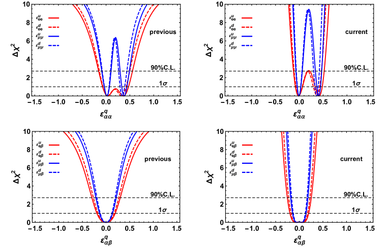
Figure 6: 1-dimensional $\Delta\chi^{2}$-distributions of neutrino-quark NSI. Note that for $\epsilon_{\mu\mu}$ the two degenerate solutions are now excluded at more than 3.5$\sigma$ with the improved QF.

IV Neutrino Non-Standard Interactions

Non-Standard Interactions (NSI) of neutrinos are among the most often considered candidates for new neutrino physics Farzan and Tortola (2018); Bhupal Dev et al. (2019). Motivated by their effects in neutrino oscillations one typically considers vector-like NSI in the form of dimension-6 operators:

$$-{\cal L}_{NSI}=\sqrt{8}\,G_{F}\,\epsilon_{\alpha\beta}^{f}\left(\bar{\nu}_{L\alpha}\gamma^{\mu}\nu_{\beta}\right)\left(\bar{f}\gamma_{\mu}f\right).$$ (22)

The dimensionless parameters fulfill $\epsilon^{f}_{\alpha\beta}=\epsilon^{f\ast}_{\beta\alpha}$. For our purposes we need to consider $f=u,d$ and can distinguish flavor-diagonal (FD) and flavor-changing (FC) NSI. The FD case is treated in Eq. (4) by making the replacement $Q_{W}^{2}\rightarrow Q_{W,\alpha\alpha}^{2}$, while for the FC case we use $Q_{W}^{2}\rightarrow Q_{W}^{2}+Q_{W,\alpha\beta}^{2}$:

$$Q_{W,\alpha\alpha}^{2} = \left[Z(g_{p}^{V}+2\varepsilon_{\alpha\alpha}^{u}+\varepsilon_{\alpha\alpha}^{d})+N(g_{n}^{V}+2\varepsilon_{\alpha\alpha}^{d}+\varepsilon_{\alpha\alpha}^{u})\,\right]^{2},$$ (23)

$$Q_{W,\alpha\beta}^{2} = \underset{\beta\neq\alpha}{\sum}\left|Z(2\varepsilon_{\alpha\beta}^{u}+\varepsilon_{\alpha\beta}^{d})+N(2\varepsilon_{\alpha\beta}^{d}+\varepsilon_{\alpha\beta}^{u})\right|^{2}.$$ (24)

Ignoring phases we explicitly write out the coupling factors for $\alpha=e$ and $\mu$:

$$Q_{W,ee}^{2} = \left[Z(g_{p}^{V}+2\varepsilon_{ee}^{u}+\varepsilon_{ee}^{d})+N(g_{n}^{V}+2\varepsilon_{ee}^{d}+\varepsilon_{ee}^{u})\,\right]^{2},$$

$$Q_{W,\mu\mu}^{2} = \left[Z(g_{p}^{V}+2\varepsilon_{\mu\mu}^{u}+\varepsilon_{\mu\mu}^{d})+N(g_{n}^{V}+2\varepsilon_{\mu\mu}^{d}+\varepsilon_{\mu\mu}^{u})\,\right]^{2},$$

$$Q_{W,e\beta}^{2} = \left[Z(2\varepsilon_{e\beta}^{u}+\varepsilon_{e\beta}^{d})+N(2\varepsilon_{e\beta}^{d}+\varepsilon_{e\beta}^{u})\,\right]^{2}\text{ (}\beta=\mu,\tau\text{)}\,,$$

$$Q_{W,\mu\beta}^{2} = \left[Z(2\varepsilon_{\mu\beta}^{u}+\varepsilon_{\mu\beta}^{d})+N(2\varepsilon_{\mu\beta}^{d}+\varepsilon_{\mu\beta}^{u})\,\right]^{2}\text{(}\beta=\mu,\tau\text{)}\,,$$

where summation over $\beta$ in the last two lines is understood.

The results of one parameter at-a-time fits for the NSI parameters are shown in Fig. 6. The bounds at 90% C.L. are

FD : $$-0.12<\varepsilon_{ee}^{u}<0.52,\ \ -0.11<\varepsilon_{ee}^{d}<0.47,\ \ -0.07<\varepsilon_{\mu\mu}^{u}<0.47,\ \ -0.06<\varepsilon_{\mu\mu}^{d}<0.42\,,$$

FC : $$-0.25<\varepsilon_{e\beta}^{u}<0.25,\ \ -0.23<\varepsilon_{e\beta}^{d}<0.23,\ \ -0.18<\varepsilon_{\mu\beta}^{u}<0.18,\ \ -0.16<\varepsilon_{\mu\beta}^{d}<0.16\,.$$

Of particular interest is a set of parameter values that would allow the LMA-Dark solution Miranda et al. (2006) with a solar neutrino mixing angle $\sin^{2}\theta_{12}>\pi/4$. It would correspond to large and negative $\epsilon_{ee}-\epsilon_{\mu\mu}=-{\cal O}(1)$. One such case is displayed in Fig. 7, compared to our fit results. A full analysis to quantify the degree with which LMA-Dark is ruled out would require fitting COHERENT data together with neutrino oscillation experiments as done in Ref. Coloma et al. (2017), and as shown there the LMA-Dark solution caused by effective operators is ruled out by COHERENT (with the previous QF) at 3$\sigma$. Here we simply take the LMA-Dark allowed parameter values and compare with our fit. One can see from Fig. 7 that the boundaries from our two-parameter fitting exclude the LMA-Dark solution at about 90% C.L. (at 2.1 $\sigma$) for the previous data (left figure), while for the new QF the exclusion occurs at more than 99% C.L. (3.1 $\sigma$).

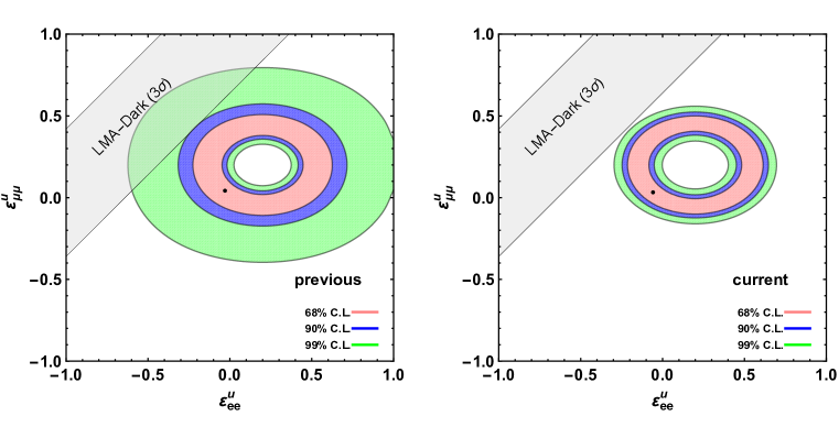
Figure 7: 2-dimensional $\Delta\chi^{2}$-contour regions of NSI parameters relevant for LMA-Dark, whose parameters have been overlaid on the COHERENT results.

V New Neutral Currents from Vector and Scalar Mediators

New neutral vector and scalar mediators may couple to neutrinos and quarks, thereby generating new neutral currents. We can write Cerdeño et al. (2016)

$${\cal L}_{vec} = g_{Z^{\prime}}\left(\bar{\nu}_{L}\gamma^{\mu}\nu_{L}+\bar{q}\gamma^{\mu}q\right)Z^{\prime}_{\mu}\,,$$ (25)

$${\cal L}_{sca} = g_{\phi}\left(\bar{\nu}_{R}\nu_{L}+\bar{q}q\right)\phi+h.c.$$ (26)

For the vector case we restrict ourselves to the simplest scenario of coupling only to the left-handed SM neutrinos. We also assume all couplings to be universal. Apart from the couplings $g_{Z^{\prime},\phi}$ we also have the masses $M_{Z^{\prime},\phi}$ as new parameters.

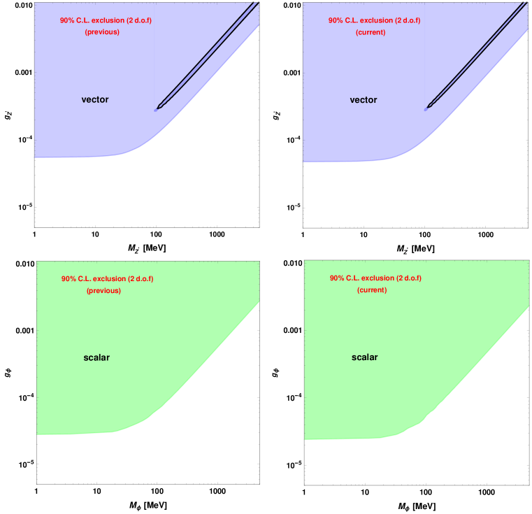
Figure 8: 2-dimensional $\Delta\chi^{2}$-contour plots at 90% C.L. for vector and scalar mediator masses and couplings with 28% (left-panels) and 13.5% systematic errors (right-panel) at 90% C.L.

We can take new vector bosons into account by replacing the SM couplings constants in Eq. (4) as ($g_{p}^{V},g_{n}^{V})\rightarrow(g_{p}^{V}+\widetilde{g}^{V},g_{n}^{V}+\widetilde{g}^{V})$, where

$$\widetilde{g}^{V}=\frac{3g_{V}^{2}}{2\sqrt{2}G_{F}(q^{2}+M_{Z^{{}^{\prime}}}^{2})}\,.$$ (27)

The scalar contribution, in turn, is added to the cross-section incoherently via the replacement $Q_{W}^{2}\rightarrow Q_{W}^{2}+Q_{sca}^{2}$, where

$$Q_{sca}^{2}=\left(\frac{g_{\phi}^{2}(14N+15.1Z)}{2\sqrt{2}G_{f}E_{\nu}(q^{2}+M_{\phi}^{2})}\right)^{2}\frac{2MT}{\left(1-\frac{MT}{2E_{\nu}^{2}}\right)}\,.$$ (28)

We take here vector and scalar weak charges in Eq. (27) and (28) from calculations given in Ref. Cerdeño et al. (2016). For COHERENT with 28% (previous) and 13.5% (current) systematic uncertainties, we show the results both for the vector and scalar masses versus the coupling constants in Fig.  8.

Improvement can be seen from the plots, and in the vector case the degeneracy region Liao and Marfatia (2017) (when $3g_{V}^{2}/M_{Z^{\prime}}^{2}=-G_{F}4\sqrt{2}(Zg_{p}^{V}+Ng_{n}^{V})/(Z+N)$) shrinks down further, but does of course not wash out completely.

VI Conclusions

Coherent elastic neutrino-nucleus scattering is an exciting new window to neutrino and neutral current physics. We investigated the effect of an improved quenching factor knowledge applied to COHERENT’s measurement of the process. Several Standard Model and beyond the Standard Model parameters were considered. Improvement is found for all parameters, demonstrating again that the process is a powerful new handle to test many scenarios. Future measurements with higher statistics will further cement this.

Note added: When this paper was finalized, Ref. Papoulias (2019) appeared, which also uses the new QF measurement to probe several parameters in and beyond the Standard Model, although with a single-bin analysis while we do the full spectral analysis. Their results results agree with the relevant parts of this work except a few cases where different approaches were adopted.