Hindsight Trust Region Policy Optimization

Hanbo Zhang1    Site Bai1    Xuguang Lan1111Corresponding Author    David Hsu2&Nanning Zheng1
1Xi’an Jiaotong University
2National University of Singapore
{zhanghanbo163, best99317}@stu.xjtu.edu.cn, xglan@xjtu.edu.cn, dyhsu@comp.nus.edu.sg, nnzheng@xjtu.edu.cn
Abstract

Reinforcement Learning (RL) with sparse rewards is a major challenge. We propose Hindsight Trust Region Policy Optimization (HTRPO), a new RL algorithm that extends the highly successful TRPO algorithm with hindsight to tackle the challenge of sparse rewards. Hindsight refers to the algorithm’s ability to learn from information across goals, including past goals not intended for the current task. We derive the hindsight form of TRPO, together with QKL, a quadratic approximation to the KL divergence constraint on the trust region. QKL reduces variance in KL divergence estimation and improves stability in policy updates. We show that HTRPO has similar convergence property as TRPO. We also present Hindsight Goal Filtering (HGF), which further improves the learning performance for suitable tasks. HTRPO has been evaluated on various sparse-reward tasks, including Atari games and simulated robot control. Results show that HTRPO consistently outperforms TRPO, as well as HPG, a state-of-the-art policy gradient algorithm for RL with sparse rewards.

1 Introduction

Reinforcement Learning (RL) has been widely investigated to solve problems from complex strategic games Mnih et al. (2015) to precise robotic control Deisenroth et al. (2013). However, current successful practice of RL in robotics relies heavily on careful and arduous reward shapingNg et al. (1999); Grzes (2017). Sparse reward, in which the agent is rewarded only upon reaching the desired goal, obviates designing a delicate reward mechanism. It also guarantees that the agent focuses on the intended task itself without any deviation. However, sparse reward diminishes the chance for policy to converge, especially in the initial random exploration stage, since the agent can hardly get positive feedbacks.

Recently, several works have been devoted to sparse-reward RL. Andrychowicz et al. (2017) proposes Hindsight Experience Replay(HER), which trains the agent with hindsight goals generated from the achieved states through the historical interactions. Such hindsight experience substantially alleviates exploration problem caused by sparse-reward settings. Rauber et al. (2019) proposes Hindsight Policy Gradient(HPG). It introduces hindsight to policy gradient, resulting in an advanced algorithm for RL with sparse reward. However, for HPG, there remain several drawbacks hindering its application in more cases. Firstly, as an extension to “vanilla” policy gradient, its performance level and sample efficiency remain limited. Secondly, it inherits the intrinsic high variance of PG methods, and the combination with hindsight data further exacerbates the learning stability.

In this paper, we propose Hindsight Trust Region Policy Optimization (HTRPO), a hindsight form of TRPO Schulman et al. (2015b), which is an advanced RL algorithm with approximately monotonic policy improvements. We prove that HTRPO theoretically inherits the convergence property of TRPO, and significantly reduces the variance of policy improvement by introducing Quadratic KL divergence Estimation (QKL) approach. Moreover, to select hindsight goals that better assist the agent to reach the original goals, we design a Hindsight Goal Filtering mechanism.

We demonstrate that in a wide variety of sparse-reward tasks including benchmark toy tasks, image-input Atari games and discrete and continuous robotic control, HTRPO can consistently outperform TRPO and HPG in the aspect of performance and sample efficiency with commendable learning stability. We also provide a comprehensive comparison with HER, showing that HTRPO achieves much better performance in 6 out of 7 benchmarks. Besides, we also conduct ablation studies to show that Quadratic KL divergence Estimation can effectively lower the variance and constrain the divergence while Hindsight Goal Filtering brings the performance to a higher level especially in more challenging tasks.

2 Preliminaries

RL Formulation and Notation.

Consider the standard infinite-horizon reinforcement learning formulation which can be defined by tuple (𝒮,𝒜,π,ρ0,r,γ)𝒮𝒜𝜋subscript𝜌0𝑟𝛾(\mathcal{S},\mathcal{A},\mathcal{\pi},\rho_{0},r,\gamma). 𝒮𝒮\mathcal{S} and 𝒜𝒜\mathcal{A} denote the set of states and actions respectively. π:𝒮𝒫(𝒜):𝜋𝒮𝒫𝒜\pi:\mathcal{S}\to\mathcal{P}(\mathcal{A}) is a policy mapping states to a distribution over actions. ρ0subscript𝜌0\rho_{0} is the distribution of the initial state s0subscript𝑠0s_{0}. Reward function r:𝒮:𝑟𝒮r:\mathcal{S}\to\mathbb{R} defines the reward obtained from the environment and γ(0,1)𝛾01\gamma\in(0,1) is a discount factor. In this paper, the policy is a differentiable function regarding parameter θ𝜃\theta. We follow the standard formalism of state-action value function Q(s,a)𝑄𝑠𝑎Q(s,a), state value function V(s)𝑉𝑠V(s) and advantage function A(s,a)𝐴𝑠𝑎A(s,a) in Sutton and Barto (2018). We also adopt the definition of γ𝛾\gamma-discounted state visitation distribution as ρθ(s)=(1γ)t=0γtP(st=s)subscript𝜌𝜃𝑠1𝛾superscriptsubscript𝑡0superscript𝛾𝑡𝑃subscript𝑠𝑡𝑠\rho_{\theta}(s)=(1-\gamma)\sum_{t=0}^{\infty}\gamma^{t}P(s_{t}=s) Ho et al. (2016). Correspondingly, γ𝛾\gamma-discounted state-action visitation distribution Ho et al. (2016), also known as occupancy measure Ho and Ermon (2016), is defined as ρθ(s,a)=ρθ(s)×πθ(a|s)subscript𝜌𝜃𝑠𝑎subscript𝜌𝜃𝑠subscript𝜋𝜃conditional𝑎𝑠\rho_{\theta}(s,a)=\rho_{\theta}(s)\times\pi_{\theta}(a|s).

Trust Region Policy Optimization(TRPO).

TRPO Schulman et al. (2015a) is an iterative trust region method that effectively optimizes policy by maximizing the per-iteration policy improvement.  The optimization problem proposed in TRPO can be formalized as follows:

maxθ𝔼s,aρθ~(s,a)[πθ(a|s)πθ~(a|s)Aθ~(s,a)]subscript𝜃subscript𝔼similar-to𝑠𝑎subscript𝜌~𝜃𝑠𝑎delimited-[]subscript𝜋𝜃conditional𝑎𝑠subscript𝜋~𝜃conditional𝑎𝑠subscript𝐴~𝜃𝑠𝑎\displaystyle\max_{\theta}\ \mathop{\mathbb{E}}_{s,a\sim\rho_{\tilde{\theta}}(s,a)}\left[\frac{\pi_{\theta}(a|s)}{\pi_{\tilde{\theta}}(a|s)}A_{\tilde{\theta}}(s,a)\right] (1)
s.t.𝔼sρθ~(s)[DKL(πθ~(a|s)||πθ(a|s))]ϵ\displaystyle s.t.\ \mathop{\mathbb{E}}_{s\sim\rho_{\tilde{\theta}}(s)}\left[D_{KL}(\pi_{\tilde{\theta}}(a|s)||\pi_{\theta}(a|s))\right]\leq\epsilon (2)

in which ρθ~(s)=t=0γtP(st=s)subscript𝜌~𝜃𝑠superscriptsubscript𝑡0superscript𝛾𝑡𝑃subscript𝑠𝑡𝑠\rho_{\tilde{\theta}}(s)=\sum_{t=0}^{\infty}\gamma^{t}P(s_{t}=s). θ𝜃\theta denotes the parameter of the new policy while θ~~𝜃\tilde{\theta} is that of the old one.

Hindsight Policy Gradient(HPG).

HPG Rauber et al. (2019) combines the idea of hindsight Andrychowicz et al. (2017) with policy gradient methods. Though goal-conditioned reinforcement learning has been explored for a long time and actively investigated in recent works Peters and Schaal (2008); Schaul et al. (2015); Veeriah et al. (2018), HPG firstly extends the idea of hindsight to goal-conditioned policy gradient and shows that the policy gradient can be computed in expectation over all goals. The goal-conditioned policy gradient is derived as follows:

θη(πθ)=𝔼g,τ[t=0T1θlogπθ(at|st,g)Aθ(st,at,g)]subscript𝜃𝜂subscript𝜋𝜃subscript𝔼𝑔𝜏delimited-[]superscriptsubscript𝑡0𝑇1subscript𝜃subscript𝜋𝜃conditionalsubscript𝑎𝑡subscript𝑠𝑡𝑔subscript𝐴𝜃subscript𝑠𝑡subscript𝑎𝑡𝑔\displaystyle\nabla_{\theta}\eta(\pi_{\theta})=\mathop{\mathbb{E}}_{g,\tau}\left[\sum_{t=0}^{T-1}\nabla_{\theta}\log\pi_{\theta}(a_{t}|s_{t},g)A_{\theta}(s_{t},a_{t},g)\right] (3)

where τpθ(τ|g)similar-to𝜏subscript𝑝𝜃conditional𝜏𝑔\tau\sim p_{\theta}(\tau|g). Then, by applying hindsight formulation, it rewrites goal-conditioned policy gradient with trajectories conditioned on achieved goal gsuperscript𝑔g^{\prime} using importance sampling to solve sparse-reward problems efficiently.

3 Hindsight Trust Region Policy Optimization

In this section, we firstly introduce Quadratic KL divergence Estimation (QKL) method, which efficiently reduces the variance of KL estimation in TRPO and results in higher learning stability. With QKL, we show that TRPO maintains the monotonically-converging property. After that, we derive the hindsight form of TRPO, called Hindsight Trust Region Policy Optimization algorithm, to tackle the severely off-policy hindsight data for better learning with sparse rewards. Specifically, the expected return and the KL divergence constraint are both modified to adapt to hindsight data with importance sampling. Benefiting from QKL, we can precisely estimate KL divergence using hindsight data while keeping the variance below a reasonable level. Intuitively, HTRPO utilizes hindsight data to estimate the objective and the constraint, and iteratively find out the local optimal policy to ensure the approximately monotonous policy improvements.

3.1 TRPO with Quadratic KL Divergence

In TRPO, the KL divergence expectation under ρθ~(s)subscript𝜌~𝜃𝑠\rho_{\tilde{\theta}}(s) is estimated by averaging values of KL divergence conditioned on collected states. However, this method is no longer valid if KL divergence cannot be analytically computed (e.g. Gaussian Mixture Model) or the state distribution changes (e.g. using hindsight data instead of the collected ones). To solve this problem, we firstly transform the KL divergence to an expectation under occupancy measure ρθ~(s,a)=ρθ~(s)×πθ~(a|s)subscript𝜌~𝜃𝑠𝑎subscript𝜌~𝜃𝑠subscript𝜋~𝜃conditional𝑎𝑠\rho_{\tilde{\theta}}(s,a)=\rho_{\tilde{\theta}}(s)\times\pi_{\tilde{\theta}}(a|s). It can be estimated using the collected state-action pairs (s,a)𝑠𝑎(s,a), no longer depending on the analytical form of KL divergence. Also, such formulation is convenient for correcting changed distribution over state and action by importance sampling, which will be discussed in section 3.2. However, it will increase the estimation variance, causing instability of training. Therefore, by making use of another f𝑓f-divergence, we propose QKL to approximate KL divergence for variance reduction, and both theoretically and practically, we prove the effectiveness of such an approximation.

Given two policies πθ~(a|s)subscript𝜋~𝜃conditional𝑎𝑠\pi_{\tilde{\theta}}(a|s) and πθ(a|s)subscript𝜋𝜃conditional𝑎𝑠\pi_{\theta}(a|s), the KL-divergence over state s𝑠s can be converted to a logarithmic form:

DKL(πθ~(a|s)||πθ(a|s))=𝔼aπθ~(a|s)[logπθ~(a|s)logπθ(a|s)]\displaystyle D_{KL}(\pi_{\tilde{\theta}}(a|s)||\pi_{\theta}(a|s))=\mathop{\mathbb{E}}_{a\sim\pi_{\tilde{\theta}}(a|s)}\left[\log\pi_{\tilde{\theta}}(a|s)-\log\pi_{\theta}(a|s)\right]

However, simply expanding the KL-divergence into logarithmic form still leaves several problems unhandled. Firstly, such formulation causes excessively high estimation variance. Secondly, such estimation of KL-divergence is of possible negativity. To overcome these two drawbacks, we propose Quadratic KL Divergence Estimation in Proposition 1 and prove that such approximation will reduce the estimation variance in Proposition 2 (detailed proof can be found in Appendix A.1 and A.2):

Proposition 1.

(Quadratic KL Divergence Estimation). For policy πθ~(a|s)subscript𝜋~𝜃conditional𝑎𝑠\pi_{\tilde{\theta}}(a|s) and πθ(a|s)subscript𝜋𝜃conditional𝑎𝑠\pi_{\theta}(a|s), and for η=πθ(a|s)πθ~(a|s)𝜂subscript𝜋𝜃conditional𝑎𝑠subscript𝜋~𝜃conditional𝑎𝑠\eta=\pi_{\theta}(a|s)-\pi_{\tilde{\theta}}(a|s),

𝔼asubscript𝔼𝑎\displaystyle\mathop{\mathbb{E}}_{a} [logπθ~(a|s)logπθ(a|s)]delimited-[]subscript𝜋~𝜃conditional𝑎𝑠subscript𝜋𝜃conditional𝑎𝑠\displaystyle\left[\log\pi_{\tilde{\theta}}(a|s)-\log\pi_{\theta}(a|s)\right]
=𝔼a[12(logπθ~(a|s)logπθ(a|s))2]+𝔼a[O(η3)]absentsubscript𝔼𝑎delimited-[]12superscriptsubscript𝜋~𝜃conditional𝑎𝑠subscript𝜋𝜃conditional𝑎𝑠2subscript𝔼𝑎delimited-[]𝑂superscript𝜂3\displaystyle=\ \mathop{\mathbb{E}}_{a}\left[\frac{1}{2}(\log\pi_{\tilde{\theta}}(a|s)-\log\pi_{\theta}(a|s))^{2}\right]+\mathop{\mathbb{E}}_{a}\left[O(\eta^{3})\right] (4)

where aπθ~(a|s)similar-to𝑎subscript𝜋~𝜃conditional𝑎𝑠a\sim\pi_{\tilde{\theta}}(a|s).

Proposition 1 demonstrates that when θ𝜃\theta and θ~~𝜃\tilde{\theta} is of limited difference, the expectation of logπθ~(a|s)logπθ(a|s)subscript𝜋~𝜃conditional𝑎𝑠subscript𝜋𝜃conditional𝑎𝑠\log\pi_{\tilde{\theta}}(a|s)-\log\pi_{\theta}(a|s) can be sufficiently estimated by the expectation of its square. In fact, 𝔼aπθ~(a|s)[12(logπθ~(a|s)logπθ(a|s))2]subscript𝔼similar-to𝑎subscript𝜋~𝜃conditional𝑎𝑠delimited-[]12superscriptsubscript𝜋~𝜃conditional𝑎𝑠subscript𝜋𝜃conditional𝑎𝑠2\mathop{\mathbb{E}}_{a\sim\pi_{\tilde{\theta}}(a|s)}\left[\frac{1}{2}(\log\pi_{\tilde{\theta}}(a|s)-\log\pi_{\theta}(a|s))^{2}\right] is an f𝑓f-divergence, where f(x)=12x(logx)2𝑓𝑥12𝑥superscript𝑥2f(x)=\frac{1}{2}x(\log x)^{2}, which we call DQKLsubscript𝐷𝑄𝐾𝐿D_{QKL} in this paper. Noticeably, though f(x)𝑓𝑥f(x) is a convex function only when x(1e,)𝑥1𝑒x\in(\frac{1}{e},\infty), and it indeed does not correspond to an f𝑓f-divergence, in our practice, πθ~(a|s)πθ(a|s)>1esubscript𝜋~𝜃conditional𝑎𝑠subscript𝜋𝜃conditional𝑎𝑠1𝑒\frac{\pi_{\tilde{\theta}}(a|s)}{\pi_{\theta}(a|s)}>\frac{1}{e} holds, hence we can define a convex function on R+superscript𝑅R^{+}: f(x)=12x(logx)2𝑓𝑥12𝑥superscript𝑥2f(x)=\frac{1}{2}x(\log x)^{2} when x(1e,)𝑥1𝑒x\in(\frac{1}{e},\infty) and x+2e𝑥2𝑒-x+\frac{2}{e} when x(0,1e]𝑥01𝑒x\in(0,\frac{1}{e}], with an unused piece defined over (0,1e]01𝑒(0,\frac{1}{e}].

Proposition 2.

(Variance of Constraint Function). For policy πθ~(a|s)subscript𝜋~𝜃conditional𝑎𝑠\pi_{\tilde{\theta}}(a|s) and πθ(a|s)subscript𝜋𝜃conditional𝑎𝑠\pi_{\theta}(a|s), let VarVar\mathrm{Var} denote the variance of a variable. For any action a𝒜𝑎𝒜a\in\mathcal{A} and any state s𝒮𝑠𝒮s\in\mathcal{S}, when logπθ~(a|s)logπθ(a|s)[0.5,0.5]subscript𝜋~𝜃conditional𝑎𝑠subscript𝜋𝜃conditional𝑎𝑠0.50.5\log\pi_{\tilde{\theta}}(a|s)-\log\pi_{\theta}(a|s)\in\left[-0.5,0.5\right], then

Varaπθ~(a|s)[(logπθ~(a|s)logπθ(a|s))22]subscriptVarsimilar-to𝑎subscript𝜋~𝜃conditional𝑎𝑠delimited-[]superscriptsubscript𝜋~𝜃conditional𝑎𝑠subscript𝜋𝜃conditional𝑎𝑠22\displaystyle\mathop{\mathrm{Var}}_{a\sim\pi_{\tilde{\theta}}(a|s)}\left[\frac{(\log\pi_{\tilde{\theta}}(a|s)-\log\pi_{\theta}(a|s))^{2}}{2}\right]
Varaπθ~(a|s)[logπθ~(a|s)logπθ(a|s)].absentsubscriptVarsimilar-to𝑎subscript𝜋~𝜃conditional𝑎𝑠delimited-[]subscript𝜋~𝜃conditional𝑎𝑠subscript𝜋𝜃conditional𝑎𝑠\displaystyle\leq\mathop{\mathrm{Var}}_{a\sim\pi_{\tilde{\theta}}(a|s)}\left[\log\pi_{\tilde{\theta}}(a|s)-\log\pi_{\theta}(a|s)\right]. (5)

Proposition 2 illustrates that there is a decrease from the variance of logπθ~(a|s)logπθ(a|s)subscript𝜋~𝜃conditional𝑎𝑠subscript𝜋𝜃conditional𝑎𝑠\log\pi_{\tilde{\theta}}(a|s)-\log\pi_{\theta}(a|s) to the variance of its square. In fact, the closer it is between θ~~𝜃\tilde{\theta} and θ𝜃\theta, the more the variance decreases. Next, we will show that with the introduction of QKL, TRPO still maintains similar convergence property.

Proposition 3.

(Policy Improvement Guarantee) Given two policies πθsubscript𝜋𝜃\pi_{\theta} and πθ~subscript𝜋~𝜃\pi_{\tilde{\theta}}, Let

s=argmaxsDTV(πθ~(a|s),πθ(a|s))superscript𝑠subscript𝑠subscript𝐷𝑇𝑉subscript𝜋~𝜃conditional𝑎𝑠subscript𝜋𝜃conditional𝑎𝑠\displaystyle s^{*}=\arg\max_{s}D_{TV}(\pi_{\tilde{\theta}}(a|s),\pi_{\theta}(a|s))

If DKL(πθ~(a|s),πθ(a|s))DQKL(πθ~(a|s),πθ(a|s))2ln2subscript𝐷𝐾𝐿subscript𝜋~𝜃conditional𝑎superscript𝑠subscript𝜋𝜃conditional𝑎superscript𝑠subscript𝐷𝑄𝐾𝐿subscript𝜋~𝜃conditional𝑎superscript𝑠subscript𝜋𝜃conditional𝑎superscript𝑠22\frac{D_{KL}(\pi_{\tilde{\theta}}(a|s^{*}),\pi_{\theta}(a|s^{*}))}{D_{QKL}(\pi_{\tilde{\theta}}(a|s^{*}),\pi_{\theta}(a|s^{*}))}\leq\frac{2}{\ln 2}, then

η(πθ)Lπθ~(πθ)CDQKLmax(πθ~(a|s),πθ(a|s))𝜂subscript𝜋𝜃subscript𝐿subscript𝜋~𝜃subscript𝜋𝜃𝐶superscriptsubscript𝐷𝑄𝐾𝐿𝑚𝑎𝑥subscript𝜋~𝜃conditional𝑎𝑠subscript𝜋𝜃conditional𝑎𝑠\displaystyle\eta(\pi_{\theta})\geq L_{\pi_{\tilde{\theta}}}(\pi_{\theta})-CD_{QKL}^{max}(\pi_{\tilde{\theta}}(a|s),\pi_{\theta}(a|s)) (6)

where

Lπθ~(πθ)=η(πθ~)+Esπθ~(s),aπθ(a|s)[Aπθ~(s,a)]subscript𝐿subscript𝜋~𝜃subscript𝜋𝜃𝜂subscript𝜋~𝜃subscript𝐸formulae-sequencesimilar-to𝑠subscript𝜋~𝜃𝑠similar-to𝑎subscript𝜋𝜃conditional𝑎𝑠delimited-[]subscript𝐴subscript𝜋~𝜃𝑠𝑎\displaystyle L_{\pi_{\tilde{\theta}}}(\pi_{\theta})=\eta(\pi_{\tilde{\theta}})+E_{s\sim\pi_{\tilde{\theta}}(s),a\sim\pi_{\theta}(a|s)}[A_{\pi_{\tilde{\theta}}}(s,a)] (7)

and η(πθ)=E[γtrt]𝜂subscript𝜋𝜃𝐸delimited-[]superscript𝛾𝑡subscript𝑟𝑡\eta(\pi_{\theta})=E\left[\sum\gamma^{t}r_{t}\right] is the expected return, C=4βγ(1γ)2𝐶4𝛽𝛾superscript1𝛾2C=\frac{4\beta\gamma}{(1-\gamma)^{2}}, β=maxs,a|Aπθ~(s,a)|𝛽𝑚𝑎subscript𝑥𝑠𝑎subscript𝐴subscript𝜋~𝜃𝑠𝑎\beta=max_{s,a}|A_{\pi_{\tilde{\theta}}}(s,a)|, DTV(p,q)=12i|piqi|subscript𝐷𝑇𝑉𝑝𝑞12subscript𝑖subscript𝑝𝑖subscript𝑞𝑖D_{TV}(p,q)=\frac{1}{2}\sum_{i}\left|p_{i}-q_{i}\right|.

The proof and detailed analysis are given in Appendix B. Intuitively, Proposition 3 means that when two policies are not far from each other, the convergence property of TRPO also holds for the QKL constraint. As a result, with Proposition 3, we can derive a new but similar monotonically-converging algorithm as in TRPO, given in Appendix B.2. By taking a series of approximation as shown in Appendix B.2, the following policy optimization problem is derived, called QKL-TRPO.

maxθ𝔼s,aρθ~(s,a)[πθ(a|s)πθ~(a|s)Aθ~(s,a)]subscript𝜃subscript𝔼similar-to𝑠𝑎subscript𝜌~𝜃𝑠𝑎delimited-[]subscript𝜋𝜃conditional𝑎𝑠subscript𝜋~𝜃conditional𝑎𝑠subscript𝐴~𝜃𝑠𝑎\displaystyle\max_{\theta}\ \mathop{\mathbb{E}}_{s,a\sim\rho_{\tilde{\theta}}(s,a)}\left[\frac{\pi_{\theta}(a|s)}{\pi_{\tilde{\theta}}(a|s)}A_{\tilde{\theta}}(s,a)\right] (1)
s.t.𝔼s,a[12(logπθ~(a|s)logπθ(a|s))2]ϵformulae-sequence𝑠𝑡subscript𝔼𝑠𝑎delimited-[]12superscriptsubscript𝜋~𝜃conditional𝑎𝑠subscript𝜋𝜃conditional𝑎𝑠2italic-ϵ\displaystyle s.t.\ \mathop{\mathbb{E}}_{s,a}\left[\frac{1}{2}(\log\pi_{\tilde{\theta}}(a|s)-\log\pi_{\theta}(a|s))^{2}\right]\leq\epsilon (8)

It is noteworthy that QKL-TRPO can be applied to policies which do not correspond to an analytic KL divergence (e.g. GMM policies). We also provide a simple analysis of QKL-TRPO compared with the original TRPO in Appendix G.1, which shows that QKL-TRPO is comparable with TRPO in a series of MuJoCo benchmarks.

3.2 Hindsight Formulation of QKL-TRPO

In this section, we derive the hindsight form of the QKL-TRPO, called Hindsight Trust Region Policy Optimization (HTRPO), to efficiently tackle severely off-policy hindsight experience and sparse-reward RL problems.

Starting from eq.1, it can be written in the following variant form:

Lθ~(θ)subscript𝐿~𝜃𝜃\displaystyle L_{\tilde{\theta}}(\theta) =𝔼τpθ~(τ)[t=0γtπθ(at|st)πθ~(at|st)Aθ~(st,at)]absentsubscript𝔼similar-to𝜏subscript𝑝~𝜃𝜏delimited-[]superscriptsubscript𝑡0superscript𝛾𝑡subscript𝜋𝜃conditionalsubscript𝑎𝑡subscript𝑠𝑡subscript𝜋~𝜃conditionalsubscript𝑎𝑡subscript𝑠𝑡subscript𝐴~𝜃subscript𝑠𝑡subscript𝑎𝑡\displaystyle=\mathop{\mathbb{E}}_{\tau\sim p_{\tilde{\theta}}(\tau)}\left[\sum_{t=0}^{\infty}\gamma^{t}\frac{\pi_{\theta}(a_{t}|s_{t})}{\pi_{\tilde{\theta}}(a_{t}|s_{t})}A_{\tilde{\theta}}(s_{t},a_{t})\right] (9)

The derivation process of this variant form is shown explicitly in Appendix C.1 and in Schulman et al. (2015a). Given the expression above, similar to eq.3, we consider the goal-conditioned objective function:

Lθ~(θ)subscript𝐿~𝜃𝜃\displaystyle L_{\tilde{\theta}}(\theta) =𝔼g,τ[t=0γtπθ(at|st,g)πθ~(at|st,g)Aθ~(st,at,g)]absentsubscript𝔼𝑔𝜏delimited-[]superscriptsubscript𝑡0superscript𝛾𝑡subscript𝜋𝜃conditionalsubscript𝑎𝑡subscript𝑠𝑡𝑔subscript𝜋~𝜃conditionalsubscript𝑎𝑡subscript𝑠𝑡𝑔subscript𝐴~𝜃subscript𝑠𝑡subscript𝑎𝑡𝑔\displaystyle=\mathop{\mathbb{E}}_{g,\tau}\left[\sum_{t=0}^{\infty}\gamma^{t}\frac{\pi_{\theta}(a_{t}|s_{t},g)}{\pi_{\tilde{\theta}}(a_{t}|s_{t},g)}A_{\tilde{\theta}}(s_{t},a_{t},g)\right] (10)

where τpθ~(τ|g)similar-to𝜏subscript𝑝~𝜃conditional𝜏𝑔\tau\sim p_{\tilde{\theta}}(\tau|g). For the record, though it seems that eq.10 makes it possible for off-policy learning, it can be used as the objective only when policy πθsubscript𝜋𝜃{\pi_{\theta}} is close to the old policy πθ~subscript𝜋~𝜃\pi_{\tilde{\theta}}, i.e. within the trust region. Using severely off-policy data like hindsight experience will make the learning process diverge. Therefore, importance sampling is integrated to correct the difference of the trajectory distribution caused by changing the goal. Based on eq.10, the following Proposition gives out the hindsight objective function conditioned on some goal gsuperscript𝑔g^{\prime} with the distribution correction derived from importance sampling.

Proposition 4.

(Hindsight Expected Return). For the original goal g𝑔g and hindsight goal gsuperscript𝑔g^{\prime}, the object function of HTRPO Lθ~(θ)subscript𝐿~𝜃𝜃L_{\tilde{\theta}}(\theta) is given by:

Lθ~(θ)=𝔼g,τ[t=0k=0tπθ~(ak|sk,g)πθ~(ak|sk,g)γtπθ(at|st,g)πθ~(at|st,g)Aθ~(st,at,g)]subscript𝐿~𝜃𝜃subscript𝔼superscript𝑔𝜏delimited-[]superscriptsubscript𝑡0superscriptsubscriptproduct𝑘0𝑡subscript𝜋~𝜃conditionalsubscript𝑎𝑘subscript𝑠𝑘superscript𝑔subscript𝜋~𝜃conditionalsubscript𝑎𝑘subscript𝑠𝑘𝑔superscript𝛾𝑡subscript𝜋𝜃conditionalsubscript𝑎𝑡subscript𝑠𝑡superscript𝑔subscript𝜋~𝜃conditionalsubscript𝑎𝑡subscript𝑠𝑡superscript𝑔subscript𝐴~𝜃subscript𝑠𝑡subscript𝑎𝑡superscript𝑔\displaystyle L_{\tilde{\theta}}(\theta)=\mathop{\mathbb{E}}_{g^{\prime},\tau}\left[\sum_{t=0}^{\infty}\prod_{k=0}^{t}\frac{\pi_{\tilde{\theta}}(a_{k}|s_{k},g^{\prime})}{\pi_{\tilde{\theta}}(a_{k}|s_{k},g)}\gamma^{t}\frac{\pi_{\theta}(a_{t}|s_{t},g^{\prime})}{\pi_{\tilde{\theta}}(a_{t}|s_{t},g^{\prime})}A_{\tilde{\theta}}(s_{t},a_{t},g^{\prime})\right]

(11)

in which τpθ(τ|g)similar-to𝜏subscript𝑝𝜃conditional𝜏𝑔\tau\sim p_{\theta}(\tau|g) and τ=s0,a0,s1,a1,,st,at𝜏subscript𝑠0subscript𝑎0subscript𝑠1subscript𝑎1subscript𝑠𝑡subscript𝑎𝑡\tau=s_{0},a_{0},s_{1},a_{1},...,s_{t},a_{t}.

Appendix C.2 presents an explicit proof of how the hindsight-form objective function derives from eq.10. In our practice, we introduce a baseline Vθ(s)subscript𝑉𝜃𝑠V_{\theta}(s) for computing the advantage Aθsubscript𝐴𝜃A_{\theta}. Though Aθsubscript𝐴𝜃A_{\theta} here can be estimated by combining per-decision return Precup et al. (2000), due to its high variance, we adopt one-step TD method instead to get Aθsubscript𝐴𝜃A_{\theta}, i.e., Aθ(s,a)=r(s,a)+γVθ(s)Vθ(s)subscript𝐴𝜃𝑠𝑎𝑟𝑠𝑎𝛾subscript𝑉𝜃superscript𝑠subscript𝑉𝜃𝑠A_{\theta}(s,a)=r(s,a)+\gamma V_{\theta}(s^{\prime})-V_{\theta}(s). Intuitively, eq.11 provides a way to compute the expected return in terms of the advantage with new-goal-conditioned hindsight experiences which are generated from interactions directed by old goals.

Next, we demonstrate that hindsight can also be introduced to the constraint function. The proof follows the methodology similar to that in Proposition 4, and is deducted explicitly in Appendix C.3.

Proposition 5.

(HTRPO Constraint Function). For the original goal g𝑔g and hindsight goal gsuperscript𝑔g^{\prime}, the constraint between policy πθ~(a|s)subscript𝜋~𝜃conditional𝑎𝑠\pi_{\tilde{\theta}}(a|s) and policy πθ(a|s)subscript𝜋𝜃conditional𝑎𝑠\pi_{\theta}(a|s) is given by:

𝔼g[𝔼τpθ(τ|g)[t=0k=0tπθ~(ak|sk,g)πθ~(ak|sk,g)γtKt]]ϵsubscript𝔼superscript𝑔delimited-[]subscript𝔼similar-to𝜏subscript𝑝𝜃conditional𝜏𝑔delimited-[]superscriptsubscript𝑡0superscriptsubscriptproduct𝑘0𝑡subscript𝜋~𝜃conditionalsubscript𝑎𝑘subscript𝑠𝑘superscript𝑔subscript𝜋~𝜃conditionalsubscript𝑎𝑘subscript𝑠𝑘𝑔superscript𝛾𝑡subscript𝐾𝑡superscriptitalic-ϵ\displaystyle\mathop{\mathbb{E}}_{g^{\prime}}\left[\mathop{\mathbb{E}}_{\tau\sim p_{\theta}(\tau|g)}\left[\sum_{t=0}^{\infty}\prod_{k=0}^{t}\frac{\pi_{\tilde{\theta}}(a_{k}|s_{k},g^{\prime})}{\pi_{\tilde{\theta}}(a_{k}|s_{k},g)}\gamma^{t}K_{t}\right]\right]\leq\epsilon^{\prime} (12)

in which ϵ=ϵ1γsuperscriptitalic-ϵitalic-ϵ1𝛾\epsilon^{\prime}=\frac{\epsilon}{1-\gamma}, and Kt=12(logπθ~(at|st,g)logπθ(at|st,g))2subscript𝐾𝑡12superscriptsubscript𝜋~𝜃conditionalsubscript𝑎𝑡subscript𝑠𝑡superscript𝑔subscript𝜋𝜃conditionalsubscript𝑎𝑡subscript𝑠𝑡superscript𝑔2K_{t}=\frac{1}{2}(\log\pi_{\tilde{\theta}}(a_{t}|s_{t},g^{\prime})-\log\pi_{\theta}(a_{t}|s_{t},g^{\prime}))^{2}.

Proposition 5 implies the practicality of using hindsight data under condition gsuperscript𝑔g^{\prime} to estimate the KL expectation. From all illustration above, we give out the final form of the optimization problem for HTRPO:

maxθ𝔼g[𝔼τpθ(τ|g)[t=0k=0tπθ~(ak|sk,g)πθ~(ak|sk,g)γtRt]]subscript𝜃subscript𝔼superscript𝑔delimited-[]subscript𝔼similar-to𝜏subscript𝑝𝜃conditional𝜏𝑔delimited-[]superscriptsubscript𝑡0superscriptsubscriptproduct𝑘0𝑡subscript𝜋~𝜃conditionalsubscript𝑎𝑘subscript𝑠𝑘superscript𝑔subscript𝜋~𝜃conditionalsubscript𝑎𝑘subscript𝑠𝑘𝑔superscript𝛾𝑡subscript𝑅𝑡\displaystyle\vspace{-20pt}\max_{\theta}\ \mathop{\mathbb{E}}_{g^{\prime}}\left[\mathop{\mathbb{E}}_{\tau\sim p_{\theta}(\tau|g)}\left[\sum_{t=0}^{\infty}\prod_{k=0}^{t}\frac{\pi_{\tilde{\theta}}(a_{k}|s_{k},g^{\prime})}{\pi_{\tilde{\theta}}(a_{k}|s_{k},g)}\gamma^{t}R_{t}\right]\right] (13)
s.t.𝔼g[𝔼τpθ(τ|g)[t=0k=0tπθ~(ak|sk,g)πθ~(ak|sk,g)γtKt]]ϵformulae-sequence𝑠𝑡subscript𝔼superscript𝑔delimited-[]subscript𝔼similar-to𝜏subscript𝑝𝜃conditional𝜏𝑔delimited-[]superscriptsubscript𝑡0superscriptsubscriptproduct𝑘0𝑡subscript𝜋~𝜃conditionalsubscript𝑎𝑘subscript𝑠𝑘superscript𝑔subscript𝜋~𝜃conditionalsubscript𝑎𝑘subscript𝑠𝑘𝑔superscript𝛾𝑡subscript𝐾𝑡superscriptitalic-ϵ\displaystyle s.t.\ \mathop{\mathbb{E}}_{g^{\prime}}\left[\mathop{\mathbb{E}}_{\tau\sim p_{\theta}(\tau|g)}\left[\sum_{t=0}^{\infty}\prod_{k=0}^{t}\frac{\pi_{\tilde{\theta}}(a_{k}|s_{k},g^{\prime})}{\pi_{\tilde{\theta}}(a_{k}|s_{k},g)}\gamma^{t}K_{t}\right]\right]\leq\epsilon^{\prime}\vspace{-10pt} (14)

where Rt=πθ(at|st,g)πθ~(at|st,g)Aθ~(st,at,g)subscript𝑅𝑡subscript𝜋𝜃conditionalsubscript𝑎𝑡subscript𝑠𝑡superscript𝑔subscript𝜋~𝜃conditionalsubscript𝑎𝑡subscript𝑠𝑡superscript𝑔subscript𝐴~𝜃subscript𝑠𝑡subscript𝑎𝑡superscript𝑔R_{t}=\frac{\pi_{\theta}(a_{t}|s_{t},g^{\prime})}{\pi_{\tilde{\theta}}(a_{t}|s_{t},g^{\prime})}A_{\tilde{\theta}}(s_{t},a_{t},g^{\prime}) and Kt=12(logπθ~(at|st,g)logπθ(at|st,g))2subscript𝐾𝑡12superscriptsubscript𝜋~𝜃conditionalsubscript𝑎𝑡subscript𝑠𝑡superscript𝑔subscript𝜋𝜃conditionalsubscript𝑎𝑡subscript𝑠𝑡superscript𝑔2K_{t}=\frac{1}{2}(\log\pi_{\tilde{\theta}}(a_{t}|s_{t},g^{\prime})-\log\pi_{\theta}(a_{t}|s_{t},g^{\prime}))^{2}. The solving process for HTRPO optimization problem is explicitly demonstrated in Appendix D.

4 Hindsight Goal Filtering

Refer to caption
Figure 1: Procedure of Hindsight Goal Filterring

In hindsight learning, the agent generalizes to reaching the original goal through learning to reach the hindsight goal first. Therefore, the selection of hindsight goals imposes a direct impact on the performance. If the hindsight goals are far from the original ones, the learned policy may not generalize well to the original goals. For example, in Fetch PickAndPlace, the initialized random policy barely grasps the target successfully, which results in the hindsight goals majorly distributing on the table. Given the original goals up in the air, such a discrepancy can cause a lower learning efficiency.

In this section, we introduce a heuristic method called Hindsight Goal Filtering(HGF). Intuitively, HGF is trying to filter the most useful goals from the achieved ones instead of random selection. Specifically, based on our analysis (eq. 13), the performance improves if we reduce the distribution discrepancy between original goals g𝑔g and hindsight goals gsuperscript𝑔g^{\prime}. Ideally, if the distribution of gsuperscript𝑔g^{\prime} matches that of g𝑔g, the agent will reach g𝑔g after learning to reach gsuperscript𝑔g^{\prime}. Therefore, we restrict the selected hindsight goals to distribute in the original goal space whenever possible to cover the area of original goals.

The main idea is shown in Figure 1 and the algorithm is summarized in Appendix E.1. The input of HGF includes 2 parts: the achieved goal set 𝒢asubscript𝒢𝑎\mathcal{G}_{a} and the original goal set 𝒢osubscript𝒢𝑜\mathcal{G}_{o}. At the beginning, especially for some complex tasks, 𝒢asubscript𝒢𝑎\mathcal{G}_{a} can only have small or even no overlap with 𝒢osubscript𝒢𝑜\mathcal{G}_{o}. Under this situation, we encourage the agent to learn to reach the original goal region by selecting the nearest achieved goals as the hindsight goals. Once some achieved goals fall in the original goal region, they are considered valid achieved goals, and a subset of this intersection will be sampled to cover the region as fully as possible. This subset is selected following the procedure in Figure 1. Note that the distance metric should be determined by the collected original goal distribution. In our experiments, we use the density-weighted Euclidean distance. Specifically, we initialize the hindsight goal set 𝒢𝒢\mathcal{G} with a randomly sampled achieved goal. To make the goal distribute dispersedly, we use Max-Min Distance as the measurement, which indicates the minimal distance between the new goal and the selected ones. By maximizing the minimal distance, it ensures an overall large distance between the new goal and the rest. HGF is related to Curriculum-guided HER (CHER)Fang et al. (2019) to some extent. However, CHER is suitable for transition-based RL, and cannot be applied to episode-based policy gradient algorithms directly.

The complete algorithm of HGF and HTRPO is presented in Appendix E.

5 Experiments

Our experiments aims to answer the following questions:

  1. 1.

    How does HTRPO compared to other methods when performed over diversified tasks?

  2. 2.

    What are the main contributors to HTRPO?

  3. 3.

    How do key parameters affect the performance?

For 1), we show that HTRPO consistently outperforms both HPG and TRPO in the aspect of success rate and sample efficiency in a wide variety of tasks, and achieves state-of-the-art performance in sparse-reward stochastic policy gradient methods. We also provide an in-depth comparison with HER in this part. For 2), we ablate the main components of HTRPO. The ablation study shows that QKL effectively reduces the variance and significantly improves the performance in all tasks. HGF plays a crucial role in improved performance for the more challenging tasks (e.g. Fetch PickAndPlace). For 3), we vary the scale of KL estimation constraint and the numbers of hindsight goals and choose the best parameter settings.

5.1 Benchmark Settings
Refer to caption
(a) Bit Flipping
Refer to caption
(b) Ms. Pacman
Refer to caption
(c) Fetch
Figure 2: Demonstration of experiment environments
Refer to caption
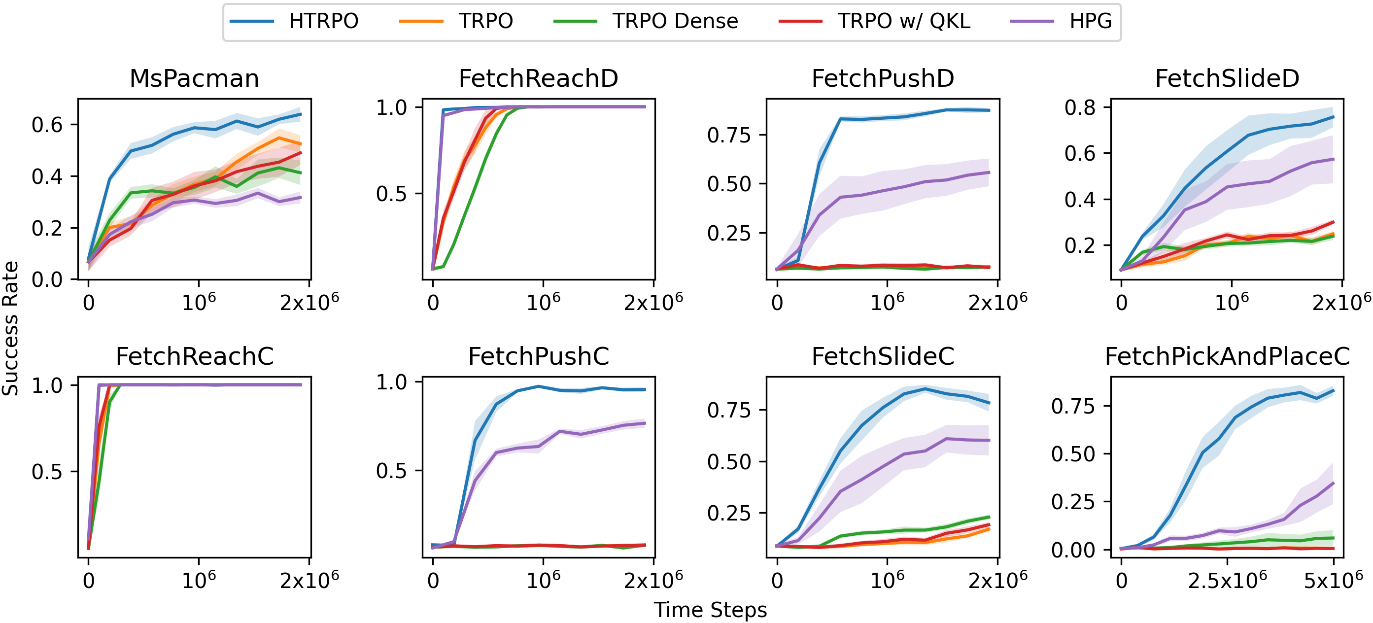
Figure 3: Success rate for benchmark environments. Top row: performance of discrete environments. Bottom row: performance of continuous environments. The full lines represent the average evaluation over 10 trails and the shaded regions represent the corresponding standard deviation.
Benchmarks

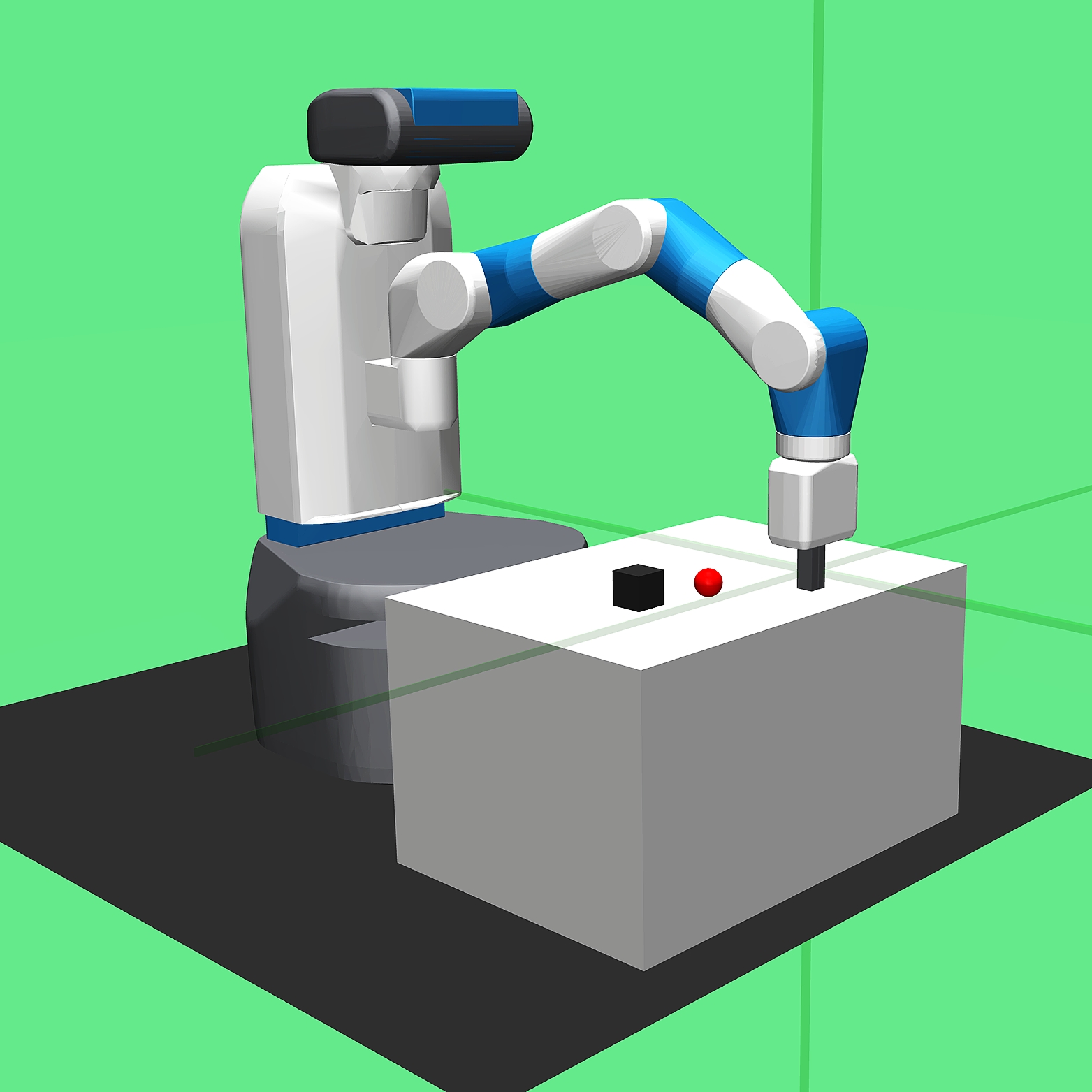
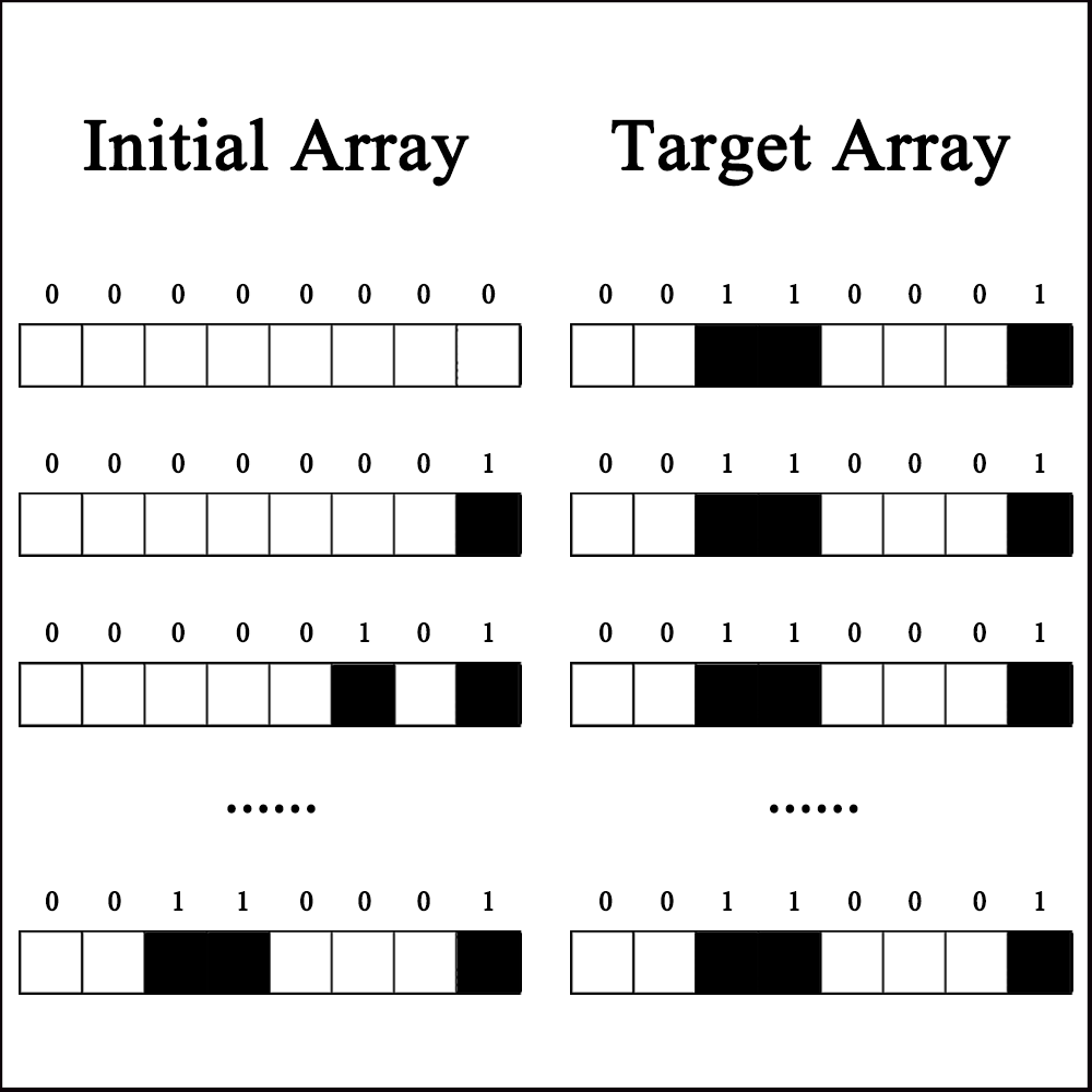
We implement HTRPO on a variety of sparse reward tasks. Firstly, we test HTRPO in simple benchmarks established in previous work Andrychowicz et al. (2017) including 4-to-100-Bit Flipping tasks. Secondly, We verify HTRPO’s performance in Atari games like Ms. Pac-Man Bellemare et al. (2013) with complex raw image input to demonstrate its generalization to convolutional neural network policies. Finally, we test HTRPO in simulated robot control tasks like Reach, Push, Slide and PickAndPlace in Fetch Plappert et al. (2018) robot environment. As mentioned in Plappert et al. (2018), it still remains unexplored that to what extent the policy gradient methods trained with hindsight data can solve continuous control tasks. Since HTRPO is a natural candidate that can be applied to both discrete and continuous tasks, other than discrete Fetch environments introduced in Rauber et al. (2019), we also implement HTRPO in continuous environments including Fetch Reach, Fetch Push, Fetch Slide, Fetch PickAndPlace.

A glimpse of these environments is demonstrated in Figure 2, and the inclusive introductions are included in Appendix F.1. Detailed settings of hyperparameters are listed in Appendix F.2. All experiments are conducted on a platform with NVIDIA GeForce GTX 1080Ti.

Baselines

We compare HTRPO with HPG Rauber et al. (2019) and TRPO Schulman et al. (2015a), which are chosen as the baseline algorithms. The reward setting used in our paper is purely sparse reward, i.e., when the task has not been finished, the agent receives 0 reward in each time step, and once the task is finished, the agent will receive a high positive reward. Besides, TRPO is also implemented with dense rewards and the new KL estimation method proposed in Section 3.1. For a fair comparison, we also combine HPG with Hindsight Goal Filtering in our experiments. To demonstrate the performance level of HTRPO more comprehensively, we also compare HTRPO with the well-known HER algorithm. In all experiments, we directly use the accumulated time steps the agent takes while interacting with the environments throughout episodes and batches, and do not count the hindsight steps which are generated using hindsight goals.

5.2 Comparative Analysis

5.2.1 How does HTRPO compared to other methods when performed over diversified tasks?

We evaluate HTRPO’s performance from success rate and sample efficiency, and test its generality to different tasks including image-based Atari games, and simulated robot control tasks. Results show HTRPO’s consistent effectiveness and strong generality to different kinds of tasks and policies.

Compare with Baselines

The success rate curves for the trained policy are demonstrated in Figure 3. We can conclude that HTRPO consistently outperforms all baselines, including different versions of TRPO and HPG, in most benchmarks, including image-based Atari games (Ms. Pac-Man) and a variety of simulated robot control tasks with different control modes. It demonstrates that HTRPO generalizes well in different kinds of tasks and policies with high-dimensional inputs. Besides, the sample efficiency of HTRPO also exceeds that of HPG, for it reaches a higher average return within less time in most environments.

Compare with HER

We implement HER with DQN Mnih et al. (2015) for discrete environments and DDPG Lillicrap et al. (2015) for continuous environments based on OpenAI baselines222https://github.com/openai/baselines. We found that HER cannot work well with the sparse reward setting of HTRPO, i.e., the reward is available only when reaching the goal. Thus, we also follow the reward setting in Andrychowicz et al. (2017) to conduct HER experiments for reference (HER-1).

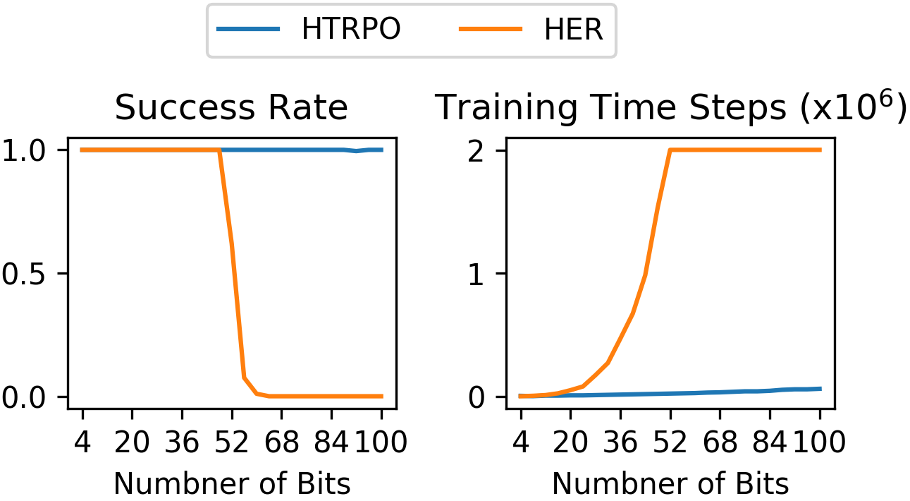
Toy Example: To begin with, we test HTRPO on 4-to-100-Bit Flipping task Andrychowicz et al. (2017) as well as HER (Figure 4). The maximum training steps are 21062superscript1062\cdot 10^{6}. In all Bit Flipping tasks, HTRPO can converge to nearly 100% success rate with much fewer time steps while HER is much data-inefficient as the number of Bits increases.

Benchmarks: Table 1 shows the comparison over the benchmark environments. We can conclude that: 1) HER can not work quite well with the purely sparse reward setting, and HTRPO outperforms HER in 6 out of 7 benchmarks significantly. 2) For discrete robot control tasks, HTRPO can learn a good policy while HER-1+DQN cannot work well. For continuous environments, HER-1 slightly outperforms HTRPO. In summary, HTRPO can be applied both in discrete and continuous tasks without any modification and achieve commendable performance compared to HER.

5.2.2 What are the main contributors to HTRPO?

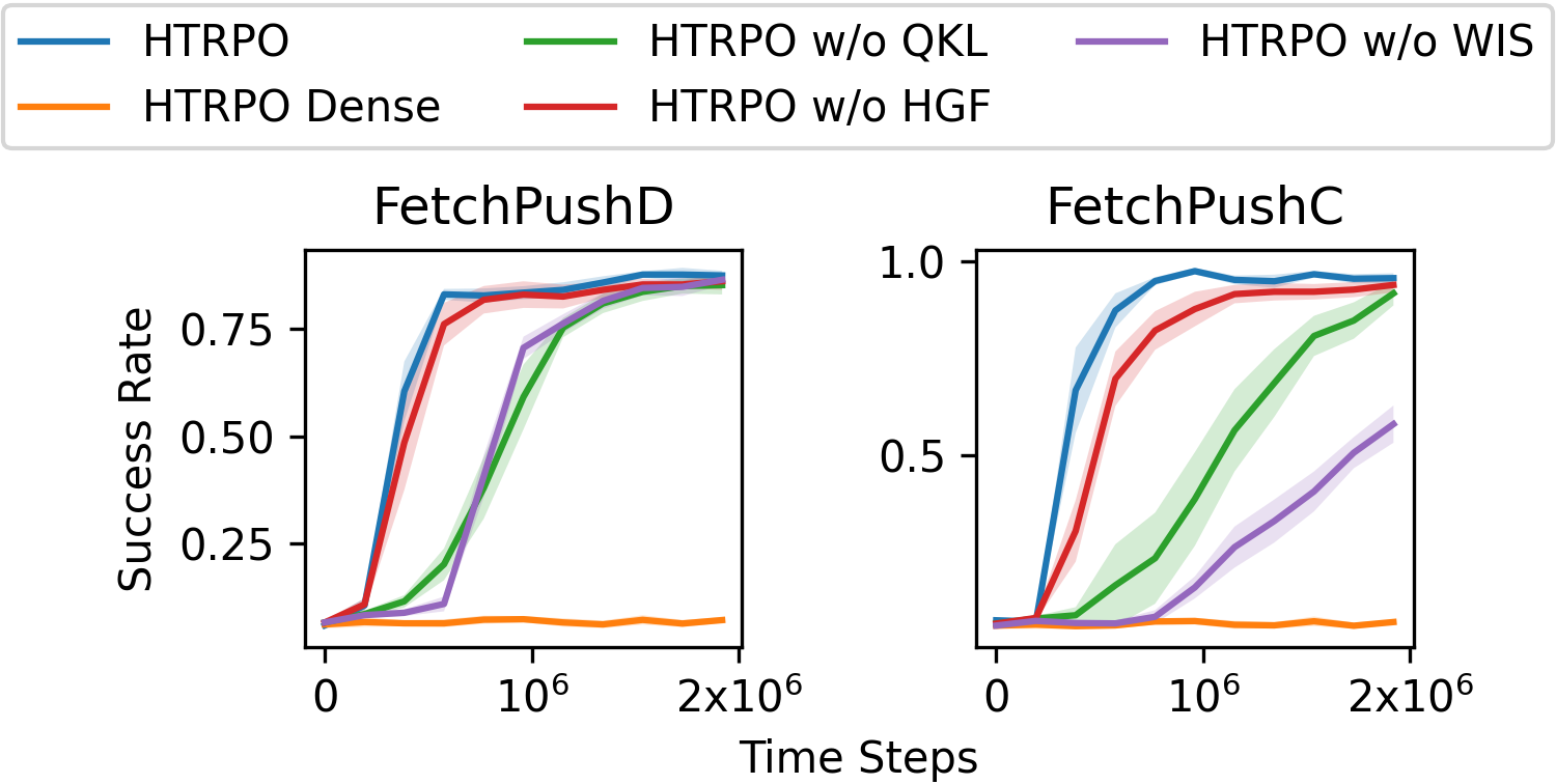
There are mainly 2 components in HTRPO, QKL and HGF, that impose an effect on the performance. Besides, we will also investigate the impact of Weighted Importance Sampling (WIS), which is conducive to variance reduction. To study the effect of reward settings, we implement HTRPO with dense rewards. Selected results are shown in Figure 5 and the full ablation study is available in Appendix G.2. We can conclude that: 1) QKL plays a crucial role for the high performance of HTRPO by significantly reducing the estimation variance of KL divergence; 2) HGF can enhance the performance of HTRPO to a higher level; 3) WIS is important since it can reduce the variance of importance sampling significantly; 4) Dense-reward setting harms the performance, which has also been verified in Plappert et al. (2018).

5.2.3 How do key parameters affect the performance?
Refer to caption
Figure 4: Performance of Bit Flipping.
Environment HER HER-1 HTRPO
Ms. Pacman 72 ±plus-or-minus\pm 3 74 ±plus-or-minus\pm 4 64 ±plus-or-minus\pm 6
Fetch Reach D 53 ±plus-or-minus\pm 41 100 ±plus-or-minus\pm 0 100 ±plus-or-minus\pm 0
Fetch Push D 8±plus-or-minus\pm1 7±plus-or-minus\pm2 88 ±plus-or-minus\pm 2
Fetch Slide D 11±plus-or-minus\pm3 10±plus-or-minus\pm5 76 ±plus-or-minus\pm 9
Fetch Reach C 18±plus-or-minus\pm3 100 ±plus-or-minus\pm 0 100 ±plus-or-minus\pm 0
Fetch Push C 7±plus-or-minus\pm2 100 ±plus-or-minus\pm 0 98 ±plus-or-minus\pm 1
Fetch Slide C 1±plus-or-minus\pm1 93 ±plus-or-minus\pm 7 85 ±plus-or-minus\pm 4
Table 1: Success rate comparison between HTRPO and HER (%). HER-1 means using the original -1-and-0 reward setting instead of the purely sparse reward that HTRPO used, i.e., only when the agent achieves the goal can it receive a high reward.

We take Continuous Fetch Push as an example to study the impact of different KL estimation constraint scales and different numbers of hindsight goals.

Different KL Estimation Constraint Scales: KL estimation constraint, i.e. max KL step specifies the trust region, the range within which the agent searches for the next-step optimal policy. In the sense of controlling the scale to which the agent updates the policy per step, this parameter presents similar functionality as learning step size. If set too low, say 5e-6 shown in Figure 6, it would inevitably slow down the converging speed. If set too high, the potentially large divergence between the new and old policy may violate the premise for some core parts of HTRPO theory derivation including Theorem 3.3 and HTRPO solving process.
Refer to caption
Figure 5: Ablation Experiments.
[Uncaptioned image]
Figure 6: Max KL steps.
[Uncaptioned image]
Figure 7: Goal numbers.

Different Number of Hindsight Goals: From the results in Figure 7, it is straightforward that more hindsight goals lead to faster converging speed. This phenomenon accords with the mechanism of how hindsight methodology deals with sparse reward scenarios, i.e. it augments the sample pool with substantial hindsight data rather than leaving it with few valid original trajectories. It’s intuitive that the more hindsight data there are, the higher sample efficiency HTRPO achieves. However, limited by the hardware resources, we need to trade off the sampled goal number.

6 Conclusion

We proposed Hindsight Trust Region Policy Optimization(HTRPO), a new RL algorithm that extends the highly successful TRPO algorithm with hindsight to tackle the challenge of sparse rewards. We show that with the help of the proposed Quadratic KL divergence Estimation (QKL), HTRPO significantly reduces the variance of KL estimation and improves the performance and learning stability. Moreover, we design a Hindsight Goal Filtering mechanism to narrow the discrepancy between hindsight and original goal space, leading to better performance. Results on diversified benchmarks demonstrate the effectiveness of HTRPO.

Since HTRPO is a natural candidate for both discrete and continuous tasks and the QKL constraint gets rid of the demand for analytical form, it is promising to optimize policies with non-Gaussian (e.g. GMM) or mixed (discrete++continuous) action space. It also provides the possibility to tackle high-dimensional real-world problems and train robot control policies without arduous reward shaping. Besides, HGF can be integrated into hindsight-goal exploration methods naturally Ren et al. (2019); Pitis et al. (2020), which should lead to a higher performance.

Acknowledgements

This work was supported in part by NSFC under grant No.91748208, No.62088102, No.61973246, Shaanxi Project under grant No.2018ZDCXLGY0607, and the program of the Ministry of Education. D. Hsu is supported by the National Research Foundation, Singapore under its AI Singapore Program (AISG Award No: AISG2-RP-2020-016).

References

  • Andrychowicz et al. [2017] Marcin Andrychowicz, Filip Wolski, Alex Ray, Jonas Schneider, Rachel Fong, Peter Welinder, Bob McGrew, Josh Tobin, Pieter Abbeel, and Wojciech Zaremba. Hindsight experience replay. In Advances in Neural Information Processing Systems, pages 5048–5058, 2017.
  • Bellemare et al. [2013] M. G. Bellemare, Y. Naddaf, J. Veness, and M. Bowling. The arcade learning environment: An evaluation platform for general agents. Journal of Artificial Intelligence Research, 47:253–279, jun 2013.
  • Boyd et al. [2004] S. Boyd, S.P. Boyd, L. Vandenberghe, and Cambridge University Press. Convex Optimization. Berichte über verteilte messysteme. Cambridge University Press, 2004.
  • Deisenroth et al. [2013] Marc Peter Deisenroth, Gerhard Neumann, Jan Peters, et al. A survey on policy search for robotics. Foundations and Trends® in Robotics, 2(1–2):1–142, 2013.
  • Fang et al. [2019] Meng Fang, Tianyi Zhou, Yali Du, Lei Han, and Zhengyou Zhang. Curriculum-guided hindsight experience replay. In Advances in Neural Information Processing Systems, pages 12623–12634, 2019.
  • Grzes [2017] Marek Grzes. Reward shaping in episodic reinforcement learning. In International Joint Conference on Autonomous Agents and Multi-agent Systems, 2017.
  • Ho and Ermon [2016] Jonathan Ho and Stefano Ermon. Generative adversarial imitation learning. In Advances in neural information processing systems, pages 4565–4573, 2016.
  • Ho et al. [2016] Jonathan Ho, Jayesh Gupta, and Stefano Ermon. Model-free imitation learning with policy optimization. In International Conference on Machine Learning, pages 2760–2769, 2016.
  • Lillicrap et al. [2015] Timothy P Lillicrap, Jonathan J Hunt, Alexander Pritzel, Nicolas Heess, Tom Erez, Yuval Tassa, David Silver, and Daan Wierstra. Continuous control with deep reinforcement learning. arXiv preprint arXiv:1509.02971, 2015.
  • Mnih et al. [2015] Volodymyr Mnih, Koray Kavukcuoglu, David Silver, Andrei A Rusu, Joel Veness, Marc G Bellemare, Alex Graves, Martin Riedmiller, Andreas K Fidjeland, Georg Ostrovski, et al. Human-level control through deep reinforcement learning. Nature, 518(7540):529, 2015.
  • Ng et al. [1999] Andrew Y Ng, Daishi Harada, and Stuart Russell. Policy invariance under reward transformations: Theory and application to reward shaping. In ICML, volume 99, pages 278–287, 1999.
  • Peters and Schaal [2008] Jan Peters and Stefan Schaal. Reinforcement learning of motor skills with policy gradients. Neural networks, 21(4):682–697, 2008.
  • Pitis et al. [2020] Silviu Pitis, Harris Chan, Stephen Zhao, Bradly Stadie, and Jimmy Ba. Maximum entropy gain exploration for long horizon multi-goal reinforcement learning. In International Conference on Machine Learning, pages 7750–7761. PMLR, 2020.
  • Plappert et al. [2018] Matthias Plappert, Marcin Andrychowicz, Alex Ray, Bob McGrew, Bowen Baker, Glenn Powell, Jonas Schneider, Josh Tobin, Maciek Chociej, Peter Welinder, et al. Multi-goal reinforcement learning: Challenging robotics environments and request for research. arXiv preprint arXiv:1802.09464, 2018.
  • Powell and Swann [1966] Michael JD Powell and J Swann. Weighted uniform sampling—a monte carlo technique for reducing variance. IMA Journal of Applied Mathematics, 2(3):228–236, 1966.
  • Precup et al. [2000] Doina Precup, Richard S Sutton, and Satinder Singh. Eligibility traces for off-policy policy evaluation. In ICML’00 Proceedings of the Seventeenth International Conference on Machine Learning, 2000.
  • Rauber et al. [2019] Paulo Rauber, Avinash Ummadisingu, Filipe Mutz, and Jürgen Schmidhuber. Hindsight policy gradients. In International Conference on Learning Representations, 2019.
  • Ren et al. [2019] Zhizhou Ren, Kefan Dong, Yuan Zhou, Qiang Liu, and Jian Peng. Exploration via hindsight goal generation. In Advances in Neural Information Processing Systems, pages 13485–13496, 2019.
  • Schaul et al. [2015] Tom Schaul, Daniel Horgan, Karol Gregor, and David Silver. Universal value function approximators. In International Conference on Machine Learning, pages 1312–1320, 2015.
  • Schulman et al. [2015a] John Schulman, Sergey Levine, Pieter Abbeel, Michael Jordan, and Philipp Moritz. Trust region policy optimization. In International Conference on Machine Learning, pages 1889–1897, 2015.
  • Schulman et al. [2015b] John Schulman, Philipp Moritz, Sergey Levine, Michael Jordan, and Pieter Abbeel. High-dimensional continuous control using generalized advantage estimation. arXiv preprint arXiv:1506.02438, 2015.
  • Sutton and Barto [2018] Ricahrd S. Sutton and Andrew G. Barto. Reinforcement Learning: An Introduction. Adaptive Computation and Machine Learning series. MIT Press, 2018.
  • Veeriah et al. [2018] Vivek Veeriah, Junhyuk Oh, and Satinder Singh. Many-goals reinforcement learning. arXiv preprint arXiv:1806.09605, 2018.

Appendix A Proof of Quadratic KL Estimation Method

A.1 Proposition 1

Lamma 1.

Given two distibutions p(x)𝑝𝑥p(x) and q(x)𝑞𝑥q(x), q(x)=p(x)+η(x)𝑞𝑥𝑝𝑥𝜂𝑥q(x)=p(x)+\eta(x), in which η(x)𝜂𝑥\eta(x) is the variation of q(x)𝑞𝑥q(x) at p(x)𝑝𝑥p(x).

𝔼[logp(x)logq(x)]𝔼delimited-[]𝑝𝑥𝑞𝑥\displaystyle\mathop{\mathbb{E}}\left[\log p(x)-\log q(x)\right]
=𝔼[12(logp(x)logq(x))2]+𝔼[o(η(x)3)]absent𝔼delimited-[]12superscript𝑝𝑥𝑞𝑥2𝔼delimited-[]𝑜𝜂superscript𝑥3\displaystyle=\mathop{\mathbb{E}}\left[\frac{1}{2}(\log p(x)-\log q(x))^{2}\right]+\mathop{\mathbb{E}}\left[o(\eta(x)^{3})\right] (15)
Proof.

Consider the second order Taylor expansion of logq(x)𝑞𝑥\log q(x) at p(x)𝑝𝑥p(x),

logq(x)=logp(x)+1p(x)η(x)12p(x)2η(x)2+o(η(x)3)𝑞𝑥𝑝𝑥1𝑝𝑥𝜂𝑥12𝑝superscript𝑥2𝜂superscript𝑥2𝑜𝜂superscript𝑥3\displaystyle\log q(x)=\log p(x)+\frac{1}{p(x)}\eta(x)-\frac{1}{2p(x)^{2}}\eta(x)^{2}+o(\eta(x)^{3}) (16)

For the left side of eq.15,

𝔼[logp(x)logq(x)]𝔼delimited-[]𝑝𝑥𝑞𝑥\displaystyle\mathop{\mathbb{E}}\left[\log p(x)-\log q(x)\right]
=𝔼[1p(x)η(x)+12p(x)2η(x)2o(η(x)3)]absent𝔼delimited-[]1𝑝𝑥𝜂𝑥12𝑝superscript𝑥2𝜂superscript𝑥2𝑜𝜂superscript𝑥3\displaystyle=\mathop{\mathbb{E}}\left[-\frac{1}{p(x)}\eta(x)+\frac{1}{2p(x)^{2}}\eta(x)^{2}-o(\eta(x)^{3})\right]
=(1p(x)η(x)+12p(x)2η(x)2o(η(x)3))p(x)𝑑xabsent1𝑝𝑥𝜂𝑥12𝑝superscript𝑥2𝜂superscript𝑥2𝑜𝜂superscript𝑥3𝑝𝑥differential-d𝑥\displaystyle=\int(-\frac{1}{p(x)}\eta(x)+\frac{1}{2p(x)^{2}}\eta(x)^{2}-o(\eta(x)^{3}))p(x)\,dx
=(12p(x)η(x)2p(x)o(η(x)3))𝑑x.absent12𝑝𝑥𝜂superscript𝑥2𝑝𝑥𝑜𝜂superscript𝑥3differential-d𝑥\displaystyle=\int(\frac{1}{2p(x)}\eta(x)^{2}-p(x)o(\eta(x)^{3}))\,dx. (17)

For the first term on the right side of eq.15,

𝔼[12(logp(x)logq(x))2]𝔼delimited-[]12superscript𝑝𝑥𝑞𝑥2\displaystyle\mathop{\mathbb{E}}\left[\frac{1}{2}(\log p(x)-\log q(x))^{2}\right]
=12𝔼[(1p(x)η(x)+12p(x)2η(x)2o(η(x)3))2]absent12𝔼delimited-[]superscript1𝑝𝑥𝜂𝑥12𝑝superscript𝑥2𝜂superscript𝑥2𝑜𝜂superscript𝑥32\displaystyle=\frac{1}{2}\mathop{\mathbb{E}}\left[(-\frac{1}{p(x)}\eta(x)+\frac{1}{2p(x)^{2}}\eta(x)^{2}-o(\eta(x)^{3}))^{2}\right]
=12𝔼[1p(x)2η(x)2+o(η(x)3)]absent12𝔼delimited-[]1𝑝superscript𝑥2𝜂superscript𝑥2𝑜𝜂superscript𝑥3\displaystyle=\frac{1}{2}\mathop{\mathbb{E}}\left[\frac{1}{p(x)^{2}}\eta(x)^{2}+o(\eta(x)^{3})\right]
=12(1p(x)2η(x)2+o(η(x)3))p(x)𝑑xabsent121𝑝superscript𝑥2𝜂superscript𝑥2𝑜𝜂superscript𝑥3𝑝𝑥differential-d𝑥\displaystyle=\frac{1}{2}\int(\frac{1}{p(x)^{2}}\eta(x)^{2}+o(\eta(x)^{3}))p(x)\,dx
=(12p(x)η(x)2+12p(x)o(η(x)3))𝑑xabsent12𝑝𝑥𝜂superscript𝑥212𝑝𝑥𝑜𝜂superscript𝑥3differential-d𝑥\displaystyle=\int(\frac{1}{2p(x)}\eta(x)^{2}+\frac{1}{2}p(x)o(\eta(x)^{3}))\,dx
=(12p(x)η(x)2p(x)o(η(x)3))𝑑x+p(x)o(η(x)3)𝑑xabsent12𝑝𝑥𝜂superscript𝑥2𝑝𝑥𝑜𝜂superscript𝑥3differential-d𝑥𝑝𝑥𝑜𝜂superscript𝑥3differential-d𝑥\displaystyle=\int(\frac{1}{2p(x)}\eta(x)^{2}-p(x)o(\eta(x)^{3}))\,dx+\int p(x)o(\eta(x)^{3})\,dx
=𝔼[logp(x)logq(x)]+𝔼[o(η(x)3)].absent𝔼delimited-[]𝑝𝑥𝑞𝑥𝔼delimited-[]𝑜𝜂superscript𝑥3\displaystyle=\mathop{\mathbb{E}}\left[\log p(x)-\log q(x)\right]+\mathop{\mathbb{E}}\left[o(\eta(x)^{3})\right]. (18)
Proposition 1.

(Approximation of Constraint Function). For policy πθ~(a|s)subscript𝜋~𝜃conditional𝑎𝑠\pi_{\tilde{\theta}}(a|s) and πθ(a|s)subscript𝜋𝜃conditional𝑎𝑠\pi_{\theta}(a|s), and for η=πθ(a|s)πθ~(a|s)𝜂subscript𝜋𝜃conditional𝑎𝑠subscript𝜋~𝜃conditional𝑎𝑠\eta=\pi_{\theta}(a|s)-\pi_{\tilde{\theta}}(a|s),

𝔼aπθ~(a|s)[logπθ~(a|s)logπθ(a|s)]subscript𝔼similar-to𝑎subscript𝜋~𝜃conditional𝑎𝑠delimited-[]subscript𝜋~𝜃conditional𝑎𝑠subscript𝜋𝜃conditional𝑎𝑠\displaystyle\mathop{\mathbb{E}}_{a\sim\pi_{\tilde{\theta}}(a|s)}\left[\log\pi_{\tilde{\theta}}(a|s)-\log\pi_{\theta}(a|s)\right]
=\displaystyle= 𝔼aπθ~(a|s)[12(logπθ~(a|s)logπθ(a|s))2]subscript𝔼similar-to𝑎subscript𝜋~𝜃conditional𝑎𝑠delimited-[]12superscriptsubscript𝜋~𝜃conditional𝑎𝑠subscript𝜋𝜃conditional𝑎𝑠2\displaystyle\ \mathop{\mathbb{E}}_{a\sim\pi_{\tilde{\theta}}(a|s)}\left[\frac{1}{2}(\log\pi_{\tilde{\theta}}(a|s)-\log\pi_{\theta}(a|s))^{2}\right]
+𝔼aπθ~(a|s)[o(η3)].subscript𝔼similar-to𝑎subscript𝜋~𝜃conditional𝑎𝑠delimited-[]𝑜superscript𝜂3\displaystyle+\mathop{\mathbb{E}}_{a\sim\pi_{\tilde{\theta}}(a|s)}\left[o(\eta^{3})\right]. (19)
Proof.

Based on Lemma 1, let p(x)=πθ~(a|s)𝑝𝑥subscript𝜋~𝜃conditional𝑎𝑠p(x)=\pi_{\tilde{\theta}}(a|s) and q(x)=πθ(a|s)𝑞𝑥subscript𝜋𝜃conditional𝑎𝑠q(x)=\pi_{\theta}(a|s), eq.15 results in eq.A.1.

A.2 Proposition 2

Lamma 2.

For any random variable Y[0,0.5]𝑌00.5Y\in\left[0,0.5\right],

Var(Y2)Var(Y),Varsuperscript𝑌2Var𝑌\displaystyle\mathrm{Var}(Y^{2})\leq\mathrm{Var}(Y), (20)

in which Var(Y)Var𝑌\mathrm{Var}(Y) denotes the variance of Y𝑌Y.

Proof.
Var(Y)Var(Y2)Var𝑌Varsuperscript𝑌2\displaystyle\mathrm{Var}(Y)-\mathrm{Var}(Y^{2})
=𝔼(Y2)[𝔼(Y)]2𝔼(Y4)+[𝔼(Y2)]2absent𝔼superscript𝑌2superscriptdelimited-[]𝔼𝑌2𝔼superscript𝑌4superscriptdelimited-[]𝔼superscript𝑌22\displaystyle=\mathop{\mathbb{E}}(Y^{2})-\left[\mathop{\mathbb{E}}(Y)\right]^{2}-\mathop{\mathbb{E}}(Y^{4})+\left[\mathop{\mathbb{E}}(Y^{2})\right]^{2}
=[𝔼(Y2)𝔼(Y4)][[𝔼(Y)]2[𝔼(Y2)]2]absentdelimited-[]𝔼superscript𝑌2𝔼superscript𝑌4delimited-[]superscriptdelimited-[]𝔼𝑌2superscriptdelimited-[]𝔼superscript𝑌22\displaystyle=\left[\mathop{\mathbb{E}}(Y^{2})-\mathop{\mathbb{E}}(Y^{4})\right]-\left[\left[\mathop{\mathbb{E}}(Y)\right]^{2}-\left[\mathop{\mathbb{E}}(Y^{2})\right]^{2}\right]
=𝔼[Y2(1Y)(1+Y)]𝔼[Y(1Y)]𝔼[Y(1+Y)]absent𝔼delimited-[]superscript𝑌21𝑌1𝑌𝔼delimited-[]𝑌1𝑌𝔼delimited-[]𝑌1𝑌\displaystyle=\mathop{\mathbb{E}}\left[Y^{2}(1-Y)(1+Y)\right]-\mathop{\mathbb{E}}\left[Y(1-Y)\right]\mathop{\mathbb{E}}\left[Y(1+Y)\right]
=Cov(Y(1+Y),Y(1Y)).absentCov𝑌1𝑌𝑌1𝑌\displaystyle=\mathrm{Cov}(Y(1+Y),Y(1-Y)). (21)

Denote X1(Y)=Y(1+Y)subscript𝑋1𝑌𝑌1𝑌X_{1}(Y)=Y(1+Y) and X2(Y)=Y(1Y)subscript𝑋2𝑌𝑌1𝑌X_{2}(Y)=Y(1-Y). Then,

Var(Y)Var(Y2)Var𝑌Varsuperscript𝑌2\displaystyle\mathrm{Var}(Y)-\mathrm{Var}(Y^{2}) =Cov(X1,X2)absentCovsubscript𝑋1subscript𝑋2\displaystyle=\mathrm{Cov}(X_{1},X_{2})
=𝔼[X1(X2𝔼(X2))]absent𝔼delimited-[]subscript𝑋1subscript𝑋2𝔼subscript𝑋2\displaystyle=\mathop{\mathbb{E}}\left[X_{1}\left(X_{2}-\mathop{\mathbb{E}}(X_{2})\right)\right] (22)

There always exists Y0[0,0.5]subscript𝑌000.5Y_{0}\in\left[0,0.5\right] that satisfies X2(Y0)=𝔼(X2)subscript𝑋2subscript𝑌0𝔼subscript𝑋2X_{2}(Y_{0})=\mathop{\mathbb{E}}(X_{2}). When Y=Y0𝑌subscript𝑌0Y=Y_{0}, let X1(Y0)=μ1subscript𝑋1subscript𝑌0subscript𝜇1X_{1}(Y_{0})=\mu_{1} in which μ1subscript𝜇1\mu_{1} is a constant. Then the equation can be converted by the following steps:

Var(Y)Var(Y2)Var𝑌Varsuperscript𝑌2\displaystyle\mathrm{Var}(Y)-\mathrm{Var}(Y^{2})
=𝔼[(X1μ1)(X2𝔼(X2))]+μ1𝔼[X2𝔼(X2)]absent𝔼delimited-[]subscript𝑋1subscript𝜇1subscript𝑋2𝔼subscript𝑋2subscript𝜇1𝔼delimited-[]subscript𝑋2𝔼subscript𝑋2\displaystyle=\mathop{\mathbb{E}}\left[\left(X_{1}-\mu_{1}\right)\left(X_{2}-\mathop{\mathbb{E}}(X_{2})\right)\right]+\mu_{1}\mathop{\mathbb{E}}\left[X_{2}-\mathop{\mathbb{E}}(X_{2})\right]
=𝔼[(X1μ1)(X2𝔼(X2))]absent𝔼delimited-[]subscript𝑋1subscript𝜇1subscript𝑋2𝔼subscript𝑋2\displaystyle=\mathop{\mathbb{E}}\left[\left(X_{1}-\mu_{1}\right)\left(X_{2}-\mathop{\mathbb{E}}(X_{2})\right)\right] (23)

Thus, when Y=Y0𝑌subscript𝑌0Y=Y_{0}, the two factors in eq.23, (X1μ1)subscript𝑋1subscript𝜇1\left(X_{1}-\mu_{1}\right) and (X2𝔼(X2))subscript𝑋2𝔼subscript𝑋2\left(X_{2}-\mathop{\mathbb{E}}(X_{2})\right) equal to 0 simultaneously.

Also, it is easy to notice that when Y[0,0.5]𝑌00.5Y\in\left[0,0.5\right], X1subscript𝑋1X_{1} and X2subscript𝑋2X_{2} are strictly increasing with the increase of Y𝑌Y. Thus, (X1μ1)subscript𝑋1subscript𝜇1\left(X_{1}-\mu_{1}\right) and (X2𝔼(X2))subscript𝑋2𝔼subscript𝑋2\left(X_{2}-\mathop{\mathbb{E}}(X_{2})\right) are either both positive or both negative, if not zero. Therefore,

Var(Y)Var(Y2)0.Var𝑌Varsuperscript𝑌20\displaystyle\mathrm{Var}(Y)-\mathrm{Var}(Y^{2})\geq 0. (24)
Lamma 3.

For any random variable Y,

Var(|Y|)Var(Y),Var𝑌Var𝑌\displaystyle\mathrm{Var}(|Y|)\leq\mathrm{Var}(Y), (25)

in which Var(Y)Var𝑌\mathrm{Var}(Y) denotes the variance of Y𝑌Y.

Proof.

Apparently,

y|f(y)|𝑑y|yf(y)𝑑y|.subscript𝑦𝑓𝑦differential-d𝑦subscript𝑦𝑓𝑦differential-d𝑦\displaystyle\int_{y}|f(y)|\,dy\geq|\int_{y}f(y)\,dy|. (26)

Consequently,

𝔼(|Y|)|𝔼(Y)|.𝔼𝑌𝔼𝑌\displaystyle\mathop{\mathbb{E}}(|Y|)\geq|\mathop{\mathbb{E}}(Y)|. (27)

For that

Var(Y)=𝔼(Y2)(𝔼(Y))2,Var𝑌𝔼superscript𝑌2superscript𝔼𝑌2\displaystyle\mathop{\mathrm{Var}}(Y)=\mathop{\mathbb{E}}(Y^{2})-(\mathop{\mathbb{E}}(Y))^{2}, (28)

we have

Var(|Y|)Var(Y).Var𝑌Var𝑌\displaystyle\mathrm{Var}(|Y|)\leq\mathrm{Var}(Y). (29)
Proposition 2.

(Variance of Constraint Function). For policy πθ~(a|s)subscript𝜋~𝜃conditional𝑎𝑠\pi_{\tilde{\theta}}(a|s) and πθ(a|s)subscript𝜋𝜃conditional𝑎𝑠\pi_{\theta}(a|s), let VarVar\mathrm{Var} denotes the variance of a variable. When logπθ~(a|s)logπθ(a|s)[0.5,0.5]subscript𝜋~𝜃conditional𝑎𝑠subscript𝜋𝜃conditional𝑎𝑠0.50.5\log\pi_{\tilde{\theta}}(a|s)-\log\pi_{\theta}(a|s)\in\left[-0.5,0.5\right], then

Varaπθ~(a|s)[(logπθ~(a|s)logπθ(a|s))22]subscriptVarsimilar-to𝑎subscript𝜋~𝜃conditional𝑎𝑠delimited-[]superscriptsubscript𝜋~𝜃conditional𝑎𝑠subscript𝜋𝜃conditional𝑎𝑠22\displaystyle\mathop{\mathrm{Var}}_{a\sim\pi_{\tilde{\theta}}(a|s)}\left[\frac{(\log\pi_{\tilde{\theta}}(a|s)-\log\pi_{\theta}(a|s))^{2}}{2}\right]
<Varaπθ~(a|s)[logπθ~(a|s)logπθ(a|s)].absentsubscriptVarsimilar-to𝑎subscript𝜋~𝜃conditional𝑎𝑠delimited-[]subscript𝜋~𝜃conditional𝑎𝑠subscript𝜋𝜃conditional𝑎𝑠\displaystyle<\mathop{\mathrm{Var}}_{a\sim\pi_{\tilde{\theta}}(a|s)}\left[\log\pi_{\tilde{\theta}}(a|s)-\log\pi_{\theta}(a|s)\right]. (30)
Proof.

let Y=|logπθ~(a|s)logπθ(a|s)|Y=|\log\pi_{\tilde{\theta}}(a|s)-\log\pi_{\theta}(a|s)|. Given Lemma 2,

Varaπθ~(a|s)[|logπθ~(a|s)logπθ(a|s)|2]\displaystyle\mathop{\mathrm{Var}}_{a\sim\pi_{\tilde{\theta}}(a|s)}\left[|\log\pi_{\tilde{\theta}}(a|s)-\log\pi_{\theta}(a|s)|^{2}\right]
Varaπθ~(a|s)[|logπθ~(a|s)logπθ(a|s)|]\displaystyle\leq\mathop{\mathrm{Var}}_{a\sim\pi_{\tilde{\theta}}(a|s)}\left[|\log\pi_{\tilde{\theta}}(a|s)-\log\pi_{\theta}(a|s)|\right] (31)

Given Lemma 3,

Varaπθ~(a|s)[|logπθ~(a|s)logπθ(a|s)|]\displaystyle\mathop{\mathrm{Var}}_{a\sim\pi_{\tilde{\theta}}(a|s)}\left[|\log\pi_{\tilde{\theta}}(a|s)-\log\pi_{\theta}(a|s)|\right]
Varaπθ~(a|s)[logπθ~(a|s)logπθ(a|s)].absentsubscriptVarsimilar-to𝑎subscript𝜋~𝜃conditional𝑎𝑠delimited-[]subscript𝜋~𝜃conditional𝑎𝑠subscript𝜋𝜃conditional𝑎𝑠\displaystyle\leq\mathop{\mathrm{Var}}_{a\sim\pi_{\tilde{\theta}}(a|s)}\left[\log\pi_{\tilde{\theta}}(a|s)-\log\pi_{\theta}(a|s)\right]. (32)

With the transitivity of inequality, combining eq.31 and eq.32, we know that

Varaπθ~(a|s)[|logπθ~(a|s)logπθ(a|s)|2]\displaystyle\mathop{\mathrm{Var}}_{a\sim\pi_{\tilde{\theta}}(a|s)}\left[|\log\pi_{\tilde{\theta}}(a|s)-\log\pi_{\theta}(a|s)|^{2}\right]
Varaπθ~(a|s)[logπθ~(a|s)logπθ(a|s)].absentsubscriptVarsimilar-to𝑎subscript𝜋~𝜃conditional𝑎𝑠delimited-[]subscript𝜋~𝜃conditional𝑎𝑠subscript𝜋𝜃conditional𝑎𝑠\displaystyle\leq\mathop{\mathrm{Var}}_{a\sim\pi_{\tilde{\theta}}(a|s)}\left[\log\pi_{\tilde{\theta}}(a|s)-\log\pi_{\theta}(a|s)\right]. (33)

Appendix B Derivation of QKL-TRPO

B.1 Proof of Proposition 3

Lamma 4.

(Policy Improvement Guarantee of TRPO) Given two policies πθsubscript𝜋𝜃\pi_{\theta} and πθ~subscript𝜋~𝜃\pi_{\tilde{\theta}}, we have:

η(πθ)Lπθ~(πθ)Cα2𝜂subscript𝜋𝜃subscript𝐿subscript𝜋~𝜃subscript𝜋𝜃𝐶superscript𝛼2\displaystyle\eta(\pi_{\theta})\geq L_{\pi_{\tilde{\theta}}}(\pi_{\theta})-C\alpha^{2} (34)

where

Lπθ~(πθ)=η(πθ~)+Esπθ~(s),aπθ(a|s)[Aπθ~(s,a)]subscript𝐿subscript𝜋~𝜃subscript𝜋𝜃𝜂subscript𝜋~𝜃subscript𝐸formulae-sequencesimilar-to𝑠subscript𝜋~𝜃𝑠similar-to𝑎subscript𝜋𝜃conditional𝑎𝑠delimited-[]subscript𝐴subscript𝜋~𝜃𝑠𝑎\displaystyle L_{\pi_{\tilde{\theta}}}(\pi_{\theta})=\eta(\pi_{\tilde{\theta}})+E_{s\sim\pi_{\tilde{\theta}}(s),a\sim\pi_{\theta}(a|s)}[A_{\pi_{\tilde{\theta}}}(s,a)] (35)

and η(πθ)=E[γtrt]𝜂subscript𝜋𝜃𝐸delimited-[]superscript𝛾𝑡subscript𝑟𝑡\eta(\pi_{\theta})=E\left[\sum\gamma^{t}r_{t}\right], C=4βγ(1γ)2𝐶4𝛽𝛾superscript1𝛾2C=\frac{4\beta\gamma}{(1-\gamma)^{2}}, β=maxs,a|Aπθ~(s,a)|𝛽𝑚𝑎subscript𝑥𝑠𝑎subscript𝐴subscript𝜋~𝜃𝑠𝑎\beta=max_{s,a}|A_{\pi_{\tilde{\theta}}}(s,a)|, α=DTVmax(πθ~(a|s),πθ(a|s))𝛼superscriptsubscript𝐷𝑇𝑉𝑚𝑎𝑥subscript𝜋~𝜃conditional𝑎𝑠subscript𝜋𝜃conditional𝑎𝑠\alpha=D_{TV}^{max}(\pi_{\tilde{\theta}}(a|s),\pi_{\theta}(a|s)).

Proof.

The detailed proof can be found in TRPOSchulman et al. [2015a].

Proposition 3.

(Policy Improvement Guarantee) Given two policies πθsubscript𝜋𝜃\pi_{\theta} and πθ~subscript𝜋~𝜃\pi_{\tilde{\theta}}, Let

s=argmaxsDTV(πθ~(a|s),πθ(a|s))superscript𝑠subscript𝑠subscript𝐷𝑇𝑉subscript𝜋~𝜃conditional𝑎𝑠subscript𝜋𝜃conditional𝑎𝑠\displaystyle s^{*}=\arg\max_{s}D_{TV}(\pi_{\tilde{\theta}}(a|s),\pi_{\theta}(a|s))

If DKL(πθ~(a|s),πθ(a|s))DQKL(πθ~(a|s),πθ(a|s))2ln2subscript𝐷𝐾𝐿subscript𝜋~𝜃conditional𝑎superscript𝑠subscript𝜋𝜃conditional𝑎superscript𝑠subscript𝐷𝑄𝐾𝐿subscript𝜋~𝜃conditional𝑎superscript𝑠subscript𝜋𝜃conditional𝑎superscript𝑠22\frac{D_{KL}(\pi_{\tilde{\theta}}(a|s^{*}),\pi_{\theta}(a|s^{*}))}{D_{QKL}(\pi_{\tilde{\theta}}(a|s^{*}),\pi_{\theta}(a|s^{*}))}\leq\frac{2}{\ln 2}, then

η(πθ)Lπθ~(πθ)CDQKLmax(πθ~(a|s),πθ(a|s))𝜂subscript𝜋𝜃subscript𝐿subscript𝜋~𝜃subscript𝜋𝜃𝐶superscriptsubscript𝐷𝑄𝐾𝐿𝑚𝑎𝑥subscript𝜋~𝜃conditional𝑎𝑠subscript𝜋𝜃conditional𝑎𝑠\displaystyle\eta(\pi_{\theta})\geq L_{\pi_{\tilde{\theta}}}(\pi_{\theta})-CD_{QKL}^{max}(\pi_{\tilde{\theta}}(a|s),\pi_{\theta}(a|s)) (36)

where

Lπθ~(πθ)=η(πθ~)+Esπθ~(s),aπθ(a|s)[Aπθ~(s,a)]subscript𝐿subscript𝜋~𝜃subscript𝜋𝜃𝜂subscript𝜋~𝜃subscript𝐸formulae-sequencesimilar-to𝑠subscript𝜋~𝜃𝑠similar-to𝑎subscript𝜋𝜃conditional𝑎𝑠delimited-[]subscript𝐴subscript𝜋~𝜃𝑠𝑎\displaystyle L_{\pi_{\tilde{\theta}}}(\pi_{\theta})=\eta(\pi_{\tilde{\theta}})+E_{s\sim\pi_{\tilde{\theta}}(s),a\sim\pi_{\theta}(a|s)}[A_{\pi_{\tilde{\theta}}}(s,a)] (37)

and η(πθ)=E[γtrt]𝜂subscript𝜋𝜃𝐸delimited-[]superscript𝛾𝑡subscript𝑟𝑡\eta(\pi_{\theta})=E\left[\sum\gamma^{t}r_{t}\right] is the expected return, C=4βγ(1γ)2𝐶4𝛽𝛾superscript1𝛾2C=\frac{4\beta\gamma}{(1-\gamma)^{2}}, β=maxs,a|Aπθ~(s,a)|𝛽𝑚𝑎subscript𝑥𝑠𝑎subscript𝐴subscript𝜋~𝜃𝑠𝑎\beta=max_{s,a}|A_{\pi_{\tilde{\theta}}}(s,a)|, DTV(p,q)=12i|piqi|subscript𝐷𝑇𝑉𝑝𝑞12subscript𝑖subscript𝑝𝑖subscript𝑞𝑖D_{TV}(p,q)=\frac{1}{2}\sum_{i}\left|p_{i}-q_{i}\right|.

Proof.

From Pinsker’s inequality, we have

DTV2(πθ~,πθ)=14πθ~πθ12ln22DKL(πθ~,πθ)superscriptsubscript𝐷𝑇𝑉2subscript𝜋~𝜃subscript𝜋𝜃14superscriptsubscriptnormsubscript𝜋~𝜃subscript𝜋𝜃1222subscript𝐷𝐾𝐿subscript𝜋~𝜃subscript𝜋𝜃\displaystyle D_{TV}^{2}(\pi_{\tilde{\theta}},\pi_{\theta})=\frac{1}{4}\left\|\pi_{\tilde{\theta}}-\pi_{\theta}\right\|_{1}^{2}\leq\frac{\ln 2}{2}D_{KL}(\pi_{\tilde{\theta}},\pi_{\theta}) (38)

Given DKL(πθ~(a|s),πθ(a|s))DQKL(πθ~(a|s),πθ(a|s))2ln2subscript𝐷𝐾𝐿subscript𝜋~𝜃conditional𝑎superscript𝑠subscript𝜋𝜃conditional𝑎superscript𝑠subscript𝐷𝑄𝐾𝐿subscript𝜋~𝜃conditional𝑎superscript𝑠subscript𝜋𝜃conditional𝑎superscript𝑠22\frac{D_{KL}(\pi_{\tilde{\theta}}(a|s^{*}),\pi_{\theta}(a|s^{*}))}{D_{QKL}(\pi_{\tilde{\theta}}(a|s^{*}),\pi_{\theta}(a|s^{*}))}\leq\frac{2}{\ln 2}, we have

DTV2(πθ~(a|s),πθ(a|s))DQKL(πθ~(a|s),πθ(a|s))superscriptsubscript𝐷𝑇𝑉2subscript𝜋~𝜃conditional𝑎superscript𝑠subscript𝜋𝜃conditional𝑎superscript𝑠subscript𝐷𝑄𝐾𝐿subscript𝜋~𝜃conditional𝑎superscript𝑠subscript𝜋𝜃conditional𝑎superscript𝑠\displaystyle D_{TV}^{2}(\pi_{\tilde{\theta}}(a|s^{*}),\pi_{\theta}(a|s^{*}))\leq D_{QKL}(\pi_{\tilde{\theta}}(a|s^{*}),\pi_{\theta}(a|s^{*})) (39)

Given Lemma 4, we have proved Proposition B.1.

B.2 Derivation of the Practical Algorithm of QKL-TRPO

To guarantee policy improvement, according to Proposition B.1, we can optimize the policy by iteratively solving the following problem (also shown in Algorithm 1:

π=argmaxπθ[Lπθ~(πθ)CDQKLmax(πθ~(a|s),πθ(a|s))]superscript𝜋subscriptsubscript𝜋𝜃subscript𝐿subscript𝜋~𝜃subscript𝜋𝜃𝐶superscriptsubscript𝐷𝑄𝐾𝐿𝑚𝑎𝑥subscript𝜋~𝜃conditional𝑎𝑠subscript𝜋𝜃conditional𝑎𝑠\pi^{*}=\arg\max_{\pi_{\theta}}\left[L_{\pi_{\tilde{\theta}}}(\pi_{\theta})-CD_{QKL}^{max}(\pi_{\tilde{\theta}}(a|s),\pi_{\theta}(a|s))\right] (40)
s.t.s=argmaxsDTV(πθ~(a|s),πθ(a|s))s.t.\quad s^{*}=\arg\max_{s}D_{TV}(\pi_{\tilde{\theta}}(a|s),\pi_{\theta}(a|s)) (41)
DKL(πθ~(a|s),πθ(a|s))DQKL(πθ~(a|s),πθ(a|s))2ln2subscript𝐷𝐾𝐿subscript𝜋~𝜃conditional𝑎superscript𝑠subscript𝜋𝜃conditional𝑎superscript𝑠subscript𝐷𝑄𝐾𝐿subscript𝜋~𝜃conditional𝑎superscript𝑠subscript𝜋𝜃conditional𝑎superscript𝑠22\quad\frac{D_{KL}(\pi_{\tilde{\theta}}(a|s^{*}),\pi_{\theta}(a|s^{*}))}{D_{QKL}(\pi_{\tilde{\theta}}(a|s^{*}),\pi_{\theta}(a|s^{*}))}\leq\frac{2}{\ln 2} (42)

where Lπθ~(πθ)=sρπθ~aπθ(a|s)Aπθ~(s,a)subscript𝐿subscript𝜋~𝜃subscript𝜋𝜃subscript𝑠subscript𝜌subscript𝜋~𝜃subscript𝑎subscript𝜋𝜃conditional𝑎𝑠subscript𝐴subscript𝜋~𝜃𝑠𝑎L_{\pi_{\tilde{\theta}}}(\pi_{\theta})=\sum_{s}\rho_{\pi_{\tilde{\theta}}}\sum_{a}\pi_{\theta}(a|s)A_{\pi_{\tilde{\theta}}}(s,a). Such an optimization results in a monotonically improvement of the policy in each optimization step since:

η(π)𝜂superscript𝜋\displaystyle\eta(\pi^{*}) Lπθ~(π)CDQKLmax(πθ~(a|s),π(a|s))absentsubscript𝐿subscript𝜋~𝜃superscript𝜋𝐶superscriptsubscript𝐷𝑄𝐾𝐿𝑚𝑎𝑥subscript𝜋~𝜃conditional𝑎𝑠superscript𝜋conditional𝑎𝑠\displaystyle\geq L_{\pi_{\tilde{\theta}}}(\pi^{*})-CD_{QKL}^{max}(\pi_{\tilde{\theta}}(a|s),\pi^{*}(a|s))
Lπθ~(πθ~)CDQKLmax(πθ~(a|s),πθ~(a|s))absentsubscript𝐿subscript𝜋~𝜃subscript𝜋~𝜃𝐶superscriptsubscript𝐷𝑄𝐾𝐿𝑚𝑎𝑥subscript𝜋~𝜃conditional𝑎𝑠subscript𝜋~𝜃conditional𝑎𝑠\displaystyle\geq L_{\pi_{\tilde{\theta}}}(\pi_{\tilde{\theta}})-CD_{QKL}^{max}(\pi_{\tilde{\theta}}(a|s),\pi_{\tilde{\theta}}(a|s))
=Lπθ~(πθ~)=η(πθ~)absentsubscript𝐿subscript𝜋~𝜃subscript𝜋~𝜃𝜂subscript𝜋~𝜃\displaystyle=L_{\pi_{\tilde{\theta}}}(\pi_{\tilde{\theta}})=\eta(\pi_{\tilde{\theta}}) (43)

As suggested in TRPO, to ensure a reasonable learning step size, we transform the penalty on DQKLmaxsuperscriptsubscript𝐷𝑄𝐾𝐿𝑚𝑎𝑥D_{QKL}^{max} to a trust region constraint:

π=argmaxπθLπθ~(πθ)superscript𝜋subscriptsubscript𝜋𝜃subscript𝐿subscript𝜋~𝜃subscript𝜋𝜃\pi^{*}=\arg\max_{\pi_{\theta}}L_{\pi_{\tilde{\theta}}}(\pi_{\theta}) (44)
s.t.s=argmaxsDTV(πθ~(a|s),πθ(a|s))s.t.\quad s^{*}=\arg\max_{s}D_{TV}(\pi_{\tilde{\theta}}(a|s),\pi_{\theta}(a|s)) (45)
DKL(πθ~(a|s),πθ(a|s))DQKL(πθ~(a|s),πθ(a|s))2ln2subscript𝐷𝐾𝐿subscript𝜋~𝜃conditional𝑎superscript𝑠subscript𝜋𝜃conditional𝑎superscript𝑠subscript𝐷𝑄𝐾𝐿subscript𝜋~𝜃conditional𝑎superscript𝑠subscript𝜋𝜃conditional𝑎superscript𝑠22\quad\frac{D_{KL}(\pi_{\tilde{\theta}}(a|s^{*}),\pi_{\theta}(a|s^{*}))}{D_{QKL}(\pi_{\tilde{\theta}}(a|s^{*}),\pi_{\theta}(a|s^{*}))}\leq\frac{2}{\ln 2} (46)
DQKLmax(πθ~(a|s),πθ(a|s))ϵ1superscriptsubscript𝐷𝑄𝐾𝐿𝑚𝑎𝑥subscript𝜋~𝜃conditional𝑎𝑠subscript𝜋𝜃conditional𝑎𝑠subscriptitalic-ϵ1\quad D_{QKL}^{max}(\pi_{\tilde{\theta}}(a|s),\pi_{\theta}(a|s))\leq\epsilon_{1} (47)

However, to solve such a constrained optimization problem, there are three difficulties: 1) the constraint represented by eq. 46 is hard to deal with; 2) it is difficult to find the point ssuperscript𝑠s^{*} that maximizes the TV divergence; 3) Eq. 47 imposes a constraint on DQKLsubscript𝐷𝑄𝐾𝐿D_{QKL} at every state, which is intractable due to the large state space.

Algorithm 1 A Monotonically-Converging Algorithm for Policy Optimization
  Initialize policy π0subscript𝜋0\pi_{0};
  i=0𝑖0i=0;
  while πisubscript𝜋𝑖\pi_{i} does not converge do
     Compute all Aπi(s,a)subscript𝐴subscript𝜋𝑖𝑠𝑎A_{\pi_{i}}(s,a);
     Solve the constrained optimization problem
     
π=argmaxπ[Lπi(π)CDQKLmax(πi(a|s),π(a|s))]superscript𝜋subscript𝜋subscript𝐿subscript𝜋𝑖𝜋𝐶superscriptsubscript𝐷𝑄𝐾𝐿𝑚𝑎𝑥subscript𝜋𝑖conditional𝑎𝑠𝜋conditional𝑎𝑠\pi^{*}=\arg\max_{\pi}\left[L_{\pi_{i}}(\pi)-CD_{QKL}^{max}(\pi_{i}(a|s),\pi(a|s))\right]
     
s.t.s=argmaxsDTV(πi(a|s),π(a|s))s.t.\quad s^{*}=\arg\max_{s}D_{TV}(\pi_{i}(a|s),\pi(a|s))
     
DKL(πi(a|s),π(a|s))DQKL(πi(a|s),π(a|s))2ln2subscript𝐷𝐾𝐿subscript𝜋𝑖conditional𝑎superscript𝑠𝜋conditional𝑎superscript𝑠subscript𝐷𝑄𝐾𝐿subscript𝜋𝑖conditional𝑎superscript𝑠𝜋conditional𝑎superscript𝑠22\quad\frac{D_{KL}(\pi_{i}(a|s^{*}),\pi(a|s^{*}))}{D_{QKL}(\pi_{i}(a|s^{*}),\pi(a|s^{*}))}\leq\frac{2}{\ln 2}
     
Lπi(π)=η(πi)+Esπi(s),aπ(a|s)[Aπi(s,a)]subscript𝐿subscript𝜋𝑖𝜋𝜂subscript𝜋𝑖subscript𝐸formulae-sequencesimilar-to𝑠subscript𝜋𝑖𝑠similar-to𝑎𝜋conditional𝑎𝑠delimited-[]subscript𝐴subscript𝜋𝑖𝑠𝑎\quad L_{\pi_{i}}(\pi)=\eta(\pi_{i})+E_{s\sim\pi_{i}(s),a\sim\pi(a|s)}[A_{\pi_{i}}(s,a)]
     i=i+1𝑖𝑖1i=i+1;
     πi=πsubscript𝜋𝑖superscript𝜋\pi_{i}=\pi^{*};
  end while
  Return πsuperscript𝜋\pi^{*}

To tackle the first two challenges, we constrain the DQKLsubscript𝐷𝑄𝐾𝐿D_{QKL} instead of the eq. 46, that is

DQKL(πθ~(a|s),πθ(a|s))ϵ2subscript𝐷𝑄𝐾𝐿subscript𝜋~𝜃conditional𝑎superscript𝑠subscript𝜋𝜃conditional𝑎superscript𝑠subscriptitalic-ϵ2D_{QKL}(\pi_{\tilde{\theta}}(a|s^{*}),\pi_{\theta}(a|s^{*}))\leq\epsilon_{2} (48)

Such a constraint is based on that limDKL0DKLDQKL=limDQKL0DKLDQKL=1subscriptsubscript𝐷𝐾𝐿0subscript𝐷𝐾𝐿subscript𝐷𝑄𝐾𝐿subscriptsubscript𝐷𝑄𝐾𝐿0subscript𝐷𝐾𝐿subscript𝐷𝑄𝐾𝐿1\lim_{D_{KL}\to 0}\frac{D_{KL}}{D_{QKL}}=\lim_{D_{QKL}\to 0}\frac{D_{KL}}{D_{QKL}}=1, i.e., for for-all\forall positive δ𝛿\delta, there exists a positive threshold ϵ2subscriptitalic-ϵ2\epsilon_{2}, when DQKLϵ2subscript𝐷𝑄𝐾𝐿subscriptitalic-ϵ2D_{QKL}\leq\epsilon_{2}, |DKLDQKL1|δsubscript𝐷𝐾𝐿subscript𝐷𝑄𝐾𝐿1𝛿\left|\frac{D_{KL}}{D_{QKL}}-1\right|\leq\delta. When δ=2ln21𝛿221\delta=\frac{2}{\ln 2}-1, we have:

22ln2DKL(πi(a|s),π(a|s))DQKL(πi(a|s),π(a|s))2ln2222subscript𝐷𝐾𝐿subscript𝜋𝑖conditional𝑎superscript𝑠𝜋conditional𝑎superscript𝑠subscript𝐷𝑄𝐾𝐿subscript𝜋𝑖conditional𝑎superscript𝑠𝜋conditional𝑎superscript𝑠222-\frac{2}{\ln 2}\leq\frac{D_{KL}(\pi_{i}(a|s^{*}),\pi(a|s^{*}))}{D_{QKL}(\pi_{i}(a|s^{*}),\pi(a|s^{*}))}\leq\frac{2}{\ln 2} (49)

which results in a stronger constraint compared with eq. 46. Intuitively, such a constraint intends to make the two policies not far from each other at a certain point ssuperscript𝑠s^{*}. Since it is hard to obtain the precise value of ϵ2subscriptitalic-ϵ2\epsilon_{2}, we set it to be a hyperparameter which controls the distance between πθ~subscript𝜋~𝜃\pi_{\tilde{\theta}} and πθsubscript𝜋𝜃\pi_{\theta}. After that, because

DQKL(πθ~(a|s),πθ(a|s))DQKLmax(πθ~(a|s),πθ(a|s))subscript𝐷𝑄𝐾𝐿subscript𝜋~𝜃conditional𝑎superscript𝑠subscript𝜋𝜃conditional𝑎superscript𝑠superscriptsubscript𝐷𝑄𝐾𝐿𝑚𝑎𝑥subscript𝜋~𝜃conditional𝑎𝑠subscript𝜋𝜃conditional𝑎𝑠D_{QKL}(\pi_{\tilde{\theta}}(a|s^{*}),\pi_{\theta}(a|s^{*}))\leq D_{QKL}^{max}(\pi_{\tilde{\theta}}(a|s),\pi_{\theta}(a|s)) (50)

obviously holds, we can further introduce a tighter constraint than eq. 48:

DQKLmax(πθ~(a|s),πθ(a|s))ϵ2superscriptsubscript𝐷𝑄𝐾𝐿𝑚𝑎𝑥subscript𝜋~𝜃conditional𝑎𝑠subscript𝜋𝜃conditional𝑎𝑠subscriptitalic-ϵ2D_{QKL}^{max}(\pi_{\tilde{\theta}}(a|s),\pi_{\theta}(a|s))\leq\epsilon_{2} (51)

which is basically the same with eq. 47 except for the constant threshold. By taking ϵ=min(ϵ1,ϵ2)italic-ϵsubscriptitalic-ϵ1subscriptitalic-ϵ2\epsilon=\min(\epsilon_{1},\epsilon_{2}), we can merge eq. 47 and 51:

π=argmaxπθLπθ~(πθ)superscript𝜋subscriptsubscript𝜋𝜃subscript𝐿subscript𝜋~𝜃subscript𝜋𝜃\pi^{*}=\arg\max_{\pi_{\theta}}L_{\pi_{\tilde{\theta}}}(\pi_{\theta}) (52)
s.t.DQKLmax(πθ~(a|s),πθ(a|s))ϵs.t.\quad D_{QKL}^{max}(\pi_{\tilde{\theta}}(a|s),\pi_{\theta}(a|s))\leq\epsilon (53)

To tackle the third challenge, inspired by TRPOSchulman et al. [2015a], we use a heuristically approximate constraint Es[DQKL(πθ~(a|s),πθ(a|s))]ϵsubscript𝐸𝑠delimited-[]subscript𝐷𝑄𝐾𝐿subscript𝜋~𝜃conditional𝑎𝑠subscript𝜋𝜃conditional𝑎𝑠italic-ϵE_{s}\left[D_{QKL}(\pi_{\tilde{\theta}}(a|s),\pi_{\theta}(a|s))\right]\leq\epsilon instead of eq. 53:

π=argmaxπθLπθ~(πθ)superscript𝜋subscriptsubscript𝜋𝜃subscript𝐿subscript𝜋~𝜃subscript𝜋𝜃\pi^{*}=\arg\max_{\pi_{\theta}}L_{\pi_{\tilde{\theta}}}(\pi_{\theta}) (54)
s.t.𝔼s[DQKL(πθ~(a|s),πθ(a|s))]ϵs.t.\quad\mathop{\mathbb{E}}_{s}\left[D_{QKL}(\pi_{\tilde{\theta}}(a|s),\pi_{\theta}(a|s))\right]\leq\epsilon (55)

This problem formulation is equivalent to:

maxθ𝔼s,aρθ~(s,a)[πθ(a|s)πθ~(a|s)Aθ~(s,a)]subscript𝜃subscript𝔼similar-to𝑠𝑎subscript𝜌~𝜃𝑠𝑎delimited-[]subscript𝜋𝜃conditional𝑎𝑠subscript𝜋~𝜃conditional𝑎𝑠subscript𝐴~𝜃𝑠𝑎\displaystyle\max_{\theta}\ \mathop{\mathbb{E}}_{s,a\sim\rho_{\tilde{\theta}}(s,a)}\left[\frac{\pi_{\theta}(a|s)}{\pi_{\tilde{\theta}}(a|s)}A_{\tilde{\theta}}(s,a)\right]
s.t.𝔼s,a[12(logπθ~(a|s)logπθ(a|s))2]ϵformulae-sequence𝑠𝑡subscript𝔼𝑠𝑎delimited-[]12superscriptsubscript𝜋~𝜃conditional𝑎𝑠subscript𝜋𝜃conditional𝑎𝑠2italic-ϵ\displaystyle s.t.\ \mathop{\mathbb{E}}_{s,a}\left[\frac{1}{2}(\log\pi_{\tilde{\theta}}(a|s)-\log\pi_{\theta}(a|s))^{2}\right]\leq\epsilon

which is called QKL-TRPO.

Appendix C Proof for Hindsight Trust Region Optimization

C.1 Reformulation of TRPO Objective

maxθ𝔼s,aρθ~(s,a)[πθ(a|s)πθ~(a|s)Aθ~(s,a)]subscript𝜃subscript𝔼similar-to𝑠𝑎subscript𝜌~𝜃𝑠𝑎delimited-[]subscript𝜋𝜃conditional𝑎𝑠subscript𝜋~𝜃conditional𝑎𝑠subscript𝐴~𝜃𝑠𝑎\displaystyle\max_{\theta}\ \mathop{\mathbb{E}}_{s,a\sim\rho_{\tilde{\theta}}(s,a)}\left[\frac{\pi_{\theta}(a|s)}{\pi_{\tilde{\theta}}(a|s)}A_{\tilde{\theta}}(s,a)\right] (56)
=maxθ𝔼τpθ~(τ)[t=0γtπθ(at|st)πθ~(at|st)Aθ~(st,at)]absentsubscript𝜃subscript𝔼similar-to𝜏subscript𝑝~𝜃𝜏delimited-[]superscriptsubscript𝑡0superscript𝛾𝑡subscript𝜋𝜃conditionalsubscript𝑎𝑡subscript𝑠𝑡subscript𝜋~𝜃conditionalsubscript𝑎𝑡subscript𝑠𝑡subscript𝐴~𝜃subscript𝑠𝑡subscript𝑎𝑡\displaystyle=\max_{\theta}\ \mathop{\mathbb{E}}_{\tau\sim p_{\tilde{\theta}}(\tau)}\left[\sum_{t=0}^{\infty}\gamma^{t}\frac{\pi_{\theta}(a_{t}|s_{t})}{\pi_{\tilde{\theta}}(a_{t}|s_{t})}A_{\tilde{\theta}}(s_{t},a_{t})\right] (57)
Proof.

With no influence to the optimal solution, we can multiply eq.56 by a constant 11γ11𝛾\frac{1}{1-\gamma},

Lθ~(θ)=11γ𝔼sρθ~,aπθ~(as)[πθ(a|s)πθ~(a|s)Aθ~(s,a)]subscript𝐿~𝜃𝜃11𝛾subscript𝔼formulae-sequencesimilar-to𝑠subscript𝜌~𝜃similar-to𝑎subscript𝜋~𝜃conditional𝑎𝑠delimited-[]subscript𝜋𝜃conditional𝑎𝑠subscript𝜋~𝜃conditional𝑎𝑠subscript𝐴~𝜃𝑠𝑎\displaystyle L_{\tilde{\theta}}(\theta)=\frac{1}{1-\gamma}\mathop{\mathbb{E}}_{s\sim\rho_{\tilde{\theta}},a\sim\pi_{\tilde{\theta}}(a\mid s)}\left[\frac{\pi_{\theta}(a|s)}{\pi_{\tilde{\theta}}(a|s)}A_{\tilde{\theta}}(s,a)\right]
=11γs𝒮t=0γtP(st=s)11γ𝔼aπθ~(a|s)[πθ(a|s)πθ~(a|s)Aθ~(s,a)]absent11𝛾subscript𝑠𝒮superscriptsubscript𝑡0superscript𝛾𝑡𝑃subscript𝑠𝑡𝑠11𝛾subscript𝔼similar-to𝑎subscript𝜋~𝜃conditional𝑎𝑠delimited-[]subscript𝜋𝜃conditional𝑎𝑠subscript𝜋~𝜃conditional𝑎𝑠subscript𝐴~𝜃𝑠𝑎\displaystyle=\frac{1}{1-\gamma}\sum_{s\in\mathcal{S}}\frac{\sum_{t=0}^{\infty}\gamma^{t}P(s_{t}=s)}{\frac{1}{1-\gamma}}\mathop{\mathbb{E}}_{a\sim\pi_{\tilde{\theta}}(a|s)}\left[\frac{\pi_{\theta}(a|s)}{\pi_{\tilde{\theta}}(a|s)}A_{\tilde{\theta}}(s,a)\right]
=t=0γt𝔼stpθ~(st),atπθ~(at|st)[πθ(at|st)πθ~(at|st)Aθ~(st,at)]absentsuperscriptsubscript𝑡0superscript𝛾𝑡subscript𝔼formulae-sequencesimilar-tosubscript𝑠𝑡subscript𝑝~𝜃subscript𝑠𝑡similar-tosubscript𝑎𝑡subscript𝜋~𝜃conditionalsubscript𝑎𝑡subscript𝑠𝑡delimited-[]subscript𝜋𝜃conditionalsubscript𝑎𝑡subscript𝑠𝑡subscript𝜋~𝜃conditionalsubscript𝑎𝑡subscript𝑠𝑡subscript𝐴~𝜃subscript𝑠𝑡subscript𝑎𝑡\displaystyle=\sum_{t=0}^{\infty}\gamma^{t}\mathop{\mathbb{E}}_{s_{t}\sim p_{\tilde{\theta}}(s_{t}),a_{t}\sim\pi_{\tilde{\theta}}(a_{t}|s_{t})}\left[\frac{\pi_{\theta}(a_{t}|s_{t})}{\pi_{\tilde{\theta}}(a_{t}|s_{t})}A_{\tilde{\theta}}(s_{t},a_{t})\right]
=𝔼τpθ~(τ)[t=0γtπθ(at|st)πθ~(at|st)Aθ~(st,at)]absentsubscript𝔼similar-to𝜏subscript𝑝~𝜃𝜏delimited-[]superscriptsubscript𝑡0superscript𝛾𝑡subscript𝜋𝜃conditionalsubscript𝑎𝑡subscript𝑠𝑡subscript𝜋~𝜃conditionalsubscript𝑎𝑡subscript𝑠𝑡subscript𝐴~𝜃subscript𝑠𝑡subscript𝑎𝑡\displaystyle=\mathop{\mathbb{E}}_{\tau\sim p_{\tilde{\theta}}(\tau)}\left[\sum_{t=0}^{\infty}\gamma^{t}\frac{\pi_{\theta}(a_{t}|s_{t})}{\pi_{\tilde{\theta}}(a_{t}|s_{t})}A_{\tilde{\theta}}(s_{t},a_{t})\right] (58)

C.2 Proposition 4

Proposition 4.

(Hindsight Expected Return). For the original goal g𝑔g and an hindsight goal gsuperscript𝑔g^{\prime}, the object function of HTRPO Lθ~(θ)subscript𝐿~𝜃𝜃L_{\tilde{\theta}}(\theta) is given by:

Lθ~(θ)subscript𝐿~𝜃𝜃\displaystyle L_{\tilde{\theta}}(\theta) =𝔼g[𝔼τpθ(τ|g)[t=0k=0tπθ~(ak|sk,g)πθ~(ak|sk,g)γtRt]]absentsubscript𝔼superscript𝑔delimited-[]subscript𝔼similar-to𝜏subscript𝑝𝜃conditional𝜏𝑔delimited-[]superscriptsubscript𝑡0superscriptsubscriptproduct𝑘0𝑡subscript𝜋~𝜃conditionalsubscript𝑎𝑘subscript𝑠𝑘superscript𝑔subscript𝜋~𝜃conditionalsubscript𝑎𝑘subscript𝑠𝑘𝑔superscript𝛾𝑡subscript𝑅𝑡\displaystyle=\mathop{\mathbb{E}}_{g^{\prime}}\left[\mathop{\mathbb{E}}_{\tau\sim p_{\theta}(\tau|g)}\left[\sum_{t=0}^{\infty}\prod_{k=0}^{t}\frac{\pi_{\tilde{\theta}}(a_{k}|s_{k},g^{\prime})}{\pi_{\tilde{\theta}}(a_{k}|s_{k},g)}\gamma^{t}R_{t}\right]\right] (59)

in which, τ=s0,a0,s1,a1,,st,at𝜏subscript𝑠0subscript𝑎0subscript𝑠1subscript𝑎1subscript𝑠𝑡subscript𝑎𝑡\tau=s_{0},a_{0},s_{1},a_{1},...,s_{t},a_{t}, and Rt=πθ(at|st,g)πθ~(at|st,g)Aθ~(st,at,g)subscript𝑅𝑡subscript𝜋𝜃conditionalsubscript𝑎𝑡subscript𝑠𝑡superscript𝑔subscript𝜋~𝜃conditionalsubscript𝑎𝑡subscript𝑠𝑡superscript𝑔subscript𝐴~𝜃subscript𝑠𝑡subscript𝑎𝑡superscript𝑔R_{t}=\frac{\pi_{\theta}(a_{t}|s_{t},g^{\prime})}{\pi_{\tilde{\theta}}(a_{t}|s_{t},g^{\prime})}A_{\tilde{\theta}}(s_{t},a_{t},g^{\prime}).

Proof.

Starting from:

Lθ~(θ)subscript𝐿~𝜃𝜃\displaystyle L_{\tilde{\theta}}(\theta) =𝔼g,τ[t=0γtπθ(at|st,g)πθ~(at|st,g)Aθ~(st,at,g)]absentsubscript𝔼𝑔𝜏delimited-[]superscriptsubscript𝑡0superscript𝛾𝑡subscript𝜋𝜃conditionalsubscript𝑎𝑡subscript𝑠𝑡𝑔subscript𝜋~𝜃conditionalsubscript𝑎𝑡subscript𝑠𝑡𝑔subscript𝐴~𝜃subscript𝑠𝑡subscript𝑎𝑡𝑔\displaystyle=\mathop{\mathbb{E}}_{g,\tau}\left[\sum_{t=0}^{\infty}\gamma^{t}\frac{\pi_{\theta}(a_{t}|s_{t},g)}{\pi_{\tilde{\theta}}(a_{t}|s_{t},g)}A_{\tilde{\theta}}(s_{t},a_{t},g)\right] (60)

for every time step t𝑡t in the expectation, denote

Lθ~(θ,t)subscript𝐿~𝜃𝜃𝑡\displaystyle L_{\tilde{\theta}}(\theta,t) =𝔼g[𝔼τpθ~(τ|g)[γtπθ(at|st,g)πθ~(at|st,g)Aθ~(st,at,g)]],absentsubscript𝔼𝑔delimited-[]subscript𝔼similar-to𝜏subscript𝑝~𝜃conditional𝜏𝑔delimited-[]superscript𝛾𝑡subscript𝜋𝜃conditionalsubscript𝑎𝑡subscript𝑠𝑡𝑔subscript𝜋~𝜃conditionalsubscript𝑎𝑡subscript𝑠𝑡𝑔subscript𝐴~𝜃subscript𝑠𝑡subscript𝑎𝑡𝑔\displaystyle=\mathop{\mathbb{E}}_{g}\left[\mathop{\mathbb{E}}_{\tau\sim p_{\tilde{\theta}}(\tau|g)}\left[\gamma^{t}\frac{\pi_{\theta}(a_{t}|s_{t},g)}{\pi_{\tilde{\theta}}(a_{t}|s_{t},g)}A_{\tilde{\theta}}(s_{t},a_{t},g)\right]\right], (61)

so that

Lθ~(θ)subscript𝐿~𝜃𝜃\displaystyle L_{\tilde{\theta}}(\theta) =t=0Lθ~(θ,t).absentsuperscriptsubscript𝑡0subscript𝐿~𝜃𝜃𝑡\displaystyle=\sum_{t=0}^{\infty}L_{\tilde{\theta}}(\theta,t). (62)

Split every trajectory τ𝜏\tau into τ1subscript𝜏1\tau_{1} and τ2subscript𝜏2\tau_{2} where τ1=s0,a0,s1,a1,,st,atsubscript𝜏1subscript𝑠0subscript𝑎0subscript𝑠1subscript𝑎1subscript𝑠𝑡subscript𝑎𝑡\tau_{1}=s_{0},a_{0},s_{1},a_{1},...,s_{t},a_{t} and τ2=st+1,at+1,subscript𝜏2subscript𝑠𝑡1subscript𝑎𝑡1\tau_{2}=s_{t+1},a_{t+1},..., then

Lθ~(θ,t)subscript𝐿~𝜃𝜃𝑡\displaystyle L_{\tilde{\theta}}(\theta,t)
=𝔼g[𝔼τ1pθ~(τ1|g)[𝔼τ2pθ~(τ2|τ1,g)[γtπθ(at|st,g)πθ~(at|st,g)Aθ~(st,at,g)]]]absentsubscript𝔼𝑔delimited-[]subscript𝔼similar-tosubscript𝜏1subscript𝑝~𝜃conditionalsubscript𝜏1𝑔delimited-[]subscript𝔼similar-tosubscript𝜏2subscript𝑝~𝜃conditionalsubscript𝜏2subscript𝜏1𝑔delimited-[]superscript𝛾𝑡subscript𝜋𝜃conditionalsubscript𝑎𝑡subscript𝑠𝑡𝑔subscript𝜋~𝜃conditionalsubscript𝑎𝑡subscript𝑠𝑡𝑔subscript𝐴~𝜃subscript𝑠𝑡subscript𝑎𝑡𝑔\displaystyle=\mathop{\mathbb{E}}_{g}\left[\mathop{\mathbb{E}}_{\tau_{1}\sim p_{\tilde{\theta}}(\tau_{1}|g)}\left[\mathop{\mathbb{E}}_{\tau_{2}\sim p_{\tilde{\theta}}(\tau_{2}|\tau_{1},g)}\left[\gamma^{t}\frac{\pi_{\theta}(a_{t}|s_{t},g)}{\pi_{\tilde{\theta}}(a_{t}|s_{t},g)}A_{\tilde{\theta}}(s_{t},a_{t},g)\right]\right]\right] (63)

For that γtπθ(at|st,g)πθ~(at|st,g)Aθ~(st,at,g)superscript𝛾𝑡subscript𝜋𝜃conditionalsubscript𝑎𝑡subscript𝑠𝑡𝑔subscript𝜋~𝜃conditionalsubscript𝑎𝑡subscript𝑠𝑡𝑔subscript𝐴~𝜃subscript𝑠𝑡subscript𝑎𝑡𝑔\gamma^{t}\frac{\pi_{\theta}(a_{t}|s_{t},g)}{\pi_{\tilde{\theta}}(a_{t}|s_{t},g)}A_{\tilde{\theta}}(s_{t},a_{t},g) is independent from τ2subscript𝜏2\tau_{2} conditioned on τ1subscript𝜏1\tau_{1},

Lθ~(θ,t)=𝔼g[𝔼τ1pθ~(τ1|g)[γtπθ(at|st,g)πθ~(at|st,g)Aθ~(st,at,g)]]subscript𝐿~𝜃𝜃𝑡subscript𝔼𝑔delimited-[]subscript𝔼similar-tosubscript𝜏1subscript𝑝~𝜃conditionalsubscript𝜏1𝑔delimited-[]superscript𝛾𝑡subscript𝜋𝜃conditionalsubscript𝑎𝑡subscript𝑠𝑡𝑔subscript𝜋~𝜃conditionalsubscript𝑎𝑡subscript𝑠𝑡𝑔subscript𝐴~𝜃subscript𝑠𝑡subscript𝑎𝑡𝑔\displaystyle L_{\tilde{\theta}}(\theta,t)=\mathop{\mathbb{E}}_{g}\left[\mathop{\mathbb{E}}_{\tau_{1}\sim p_{\tilde{\theta}}(\tau_{1}|g)}\left[\gamma^{t}\frac{\pi_{\theta}(a_{t}|s_{t},g)}{\pi_{\tilde{\theta}}(a_{t}|s_{t},g)}A_{\tilde{\theta}}(s_{t},a_{t},g)\right]\ \right]

Thus,

Lθ~(θ)subscript𝐿~𝜃𝜃\displaystyle L_{\tilde{\theta}}(\theta) =t=0𝔼g[𝔼τ1pθ~(τ1|g)[γtπθ(at|st,g)πθ~(at|st,g)Aθ~(st,at,g)]]absentsuperscriptsubscript𝑡0subscript𝔼𝑔delimited-[]subscript𝔼similar-tosubscript𝜏1subscript𝑝~𝜃conditionalsubscript𝜏1𝑔delimited-[]superscript𝛾𝑡subscript𝜋𝜃conditionalsubscript𝑎𝑡subscript𝑠𝑡𝑔subscript𝜋~𝜃conditionalsubscript𝑎𝑡subscript𝑠𝑡𝑔subscript𝐴~𝜃subscript𝑠𝑡subscript𝑎𝑡𝑔\displaystyle=\sum_{t=0}^{\infty}\mathop{\mathbb{E}}_{g}\left[\mathop{\mathbb{E}}_{\tau_{1}\sim p_{\tilde{\theta}}(\tau_{1}|g)}\left[\gamma^{t}\frac{\pi_{\theta}(a_{t}|s_{t},g)}{\pi_{\tilde{\theta}}(a_{t}|s_{t},g)}A_{\tilde{\theta}}(s_{t},a_{t},g)\right]\ \right] (64)

Following the techniques of importance sampling, the objective function can be rewritten in the form of new goal gsuperscript𝑔g^{\prime} :

Lθ~(θ)subscript𝐿~𝜃𝜃\displaystyle L_{\tilde{\theta}}(\theta) =t=0𝔼g[𝔼τ1pθ~(τ1|g)[pθ~(s0:t,a0:t|g)pθ~(s0:t,a0:t|g)γtRt]].absentsuperscriptsubscript𝑡0subscript𝔼superscript𝑔delimited-[]subscript𝔼similar-tosubscript𝜏1subscript𝑝~𝜃conditionalsubscript𝜏1𝑔delimited-[]subscript𝑝~𝜃subscript𝑠:0𝑡conditionalsubscript𝑎:0𝑡superscript𝑔subscript𝑝~𝜃subscript𝑠:0𝑡conditionalsubscript𝑎:0𝑡𝑔superscript𝛾𝑡subscript𝑅𝑡\displaystyle=\sum_{t=0}^{\infty}\mathop{\mathbb{E}}_{g^{\prime}}\left[\mathop{\mathbb{E}}_{\tau_{1}\sim p_{\tilde{\theta}}(\tau_{1}|g)}\left[\frac{p_{\tilde{\theta}}(s_{0:t},a_{0:t}|g^{\prime})}{p_{\tilde{\theta}}(s_{0:t},a_{0:t}|g)}\gamma^{t}R_{t}\right]\ \right]. (65)

where Rt=πθ(at|st,g)πθ~(at|st,g)Aθ~(st,at,g)subscript𝑅𝑡subscript𝜋𝜃conditionalsubscript𝑎𝑡subscript𝑠𝑡superscript𝑔subscript𝜋~𝜃conditionalsubscript𝑎𝑡subscript𝑠𝑡superscript𝑔subscript𝐴~𝜃subscript𝑠𝑡subscript𝑎𝑡superscript𝑔R_{t}=\frac{\pi_{\theta}(a_{t}|s_{t},g^{\prime})}{\pi_{\tilde{\theta}}(a_{t}|s_{t},g^{\prime})}A_{\tilde{\theta}}(s_{t},a_{t},g^{\prime}). Furthermore, given that

p(s0:t,a0:t|g)=p(s0)p(at|st,g)k=0t1p(ak|sk,g)p(sk+1|sk,ak),𝑝subscript𝑠:0𝑡conditionalsubscript𝑎:0𝑡𝑔𝑝subscript𝑠0𝑝conditionalsubscript𝑎𝑡subscript𝑠𝑡𝑔superscriptsubscriptproduct𝑘0𝑡1𝑝conditionalsubscript𝑎𝑘subscript𝑠𝑘𝑔𝑝conditionalsubscript𝑠𝑘1subscript𝑠𝑘subscript𝑎𝑘\displaystyle p(s_{0:t},a_{0:t}|g)=p(s_{0})p(a_{t}|s_{t},g)\prod_{k=0}^{t-1}p(a_{k}|s_{k},g)p(s_{k+1}|s_{k},a_{k}), (66)

after expanding the objective function and cancelling terms,

Lθ~(θ)subscript𝐿~𝜃𝜃\displaystyle L_{\tilde{\theta}}(\theta) =t=0𝔼g[𝔼τ1pθ~(τ1|g)[k=0tπθ~(ak|sk,g)πθ~(ak|sk,g)γtRt]]absentsuperscriptsubscript𝑡0subscript𝔼superscript𝑔delimited-[]subscript𝔼similar-tosubscript𝜏1subscript𝑝~𝜃conditionalsubscript𝜏1𝑔delimited-[]superscriptsubscriptproduct𝑘0𝑡subscript𝜋~𝜃conditionalsubscript𝑎𝑘subscript𝑠𝑘superscript𝑔subscript𝜋~𝜃conditionalsubscript𝑎𝑘subscript𝑠𝑘𝑔superscript𝛾𝑡subscript𝑅𝑡\displaystyle=\sum_{t=0}^{\infty}\mathop{\mathbb{E}}_{g^{\prime}}\left[\mathop{\mathbb{E}}_{\tau_{1}\sim p_{\tilde{\theta}}(\tau_{1}|g)}\left[\prod_{k=0}^{t}\frac{\pi_{\tilde{\theta}}(a_{k}|s_{k},g^{\prime})}{\pi_{\tilde{\theta}}(a_{k}|s_{k},g)}\gamma^{t}R_{t}\right]\right]

C.3 Proposition 5

Proposition 5.

(Quadratic KL divergence Estimation). For the original goal g𝑔g and a hindsight goal gsuperscript𝑔g^{\prime}, the constraint between policy πθ~(a|s)subscript𝜋~𝜃conditional𝑎𝑠\pi_{\tilde{\theta}}(a|s) and policy πθ(a|s)subscript𝜋𝜃conditional𝑎𝑠\pi_{\theta}(a|s) is given by:

𝔼g[𝔼τpθ(τ|g)[t=0k=1tπθ~(ak|sk,g)πθ~(ak|sk,g)γtKt]]ϵsubscript𝔼superscript𝑔delimited-[]subscript𝔼similar-to𝜏subscript𝑝𝜃conditional𝜏𝑔delimited-[]superscriptsubscript𝑡0superscriptsubscriptproduct𝑘1𝑡subscript𝜋~𝜃conditionalsubscript𝑎𝑘subscript𝑠𝑘superscript𝑔subscript𝜋~𝜃conditionalsubscript𝑎𝑘subscript𝑠𝑘𝑔superscript𝛾𝑡subscript𝐾𝑡superscriptitalic-ϵ\displaystyle\mathop{\mathbb{E}}_{g^{\prime}}\left[\mathop{\mathbb{E}}_{\tau\sim p_{\theta}(\tau|g)}\left[\sum_{t=0}^{\infty}\prod_{k=1}^{t}\frac{\pi_{\tilde{\theta}}(a_{k}|s_{k},g^{\prime})}{\pi_{\tilde{\theta}}(a_{k}|s_{k},g)}\gamma^{t}K_{t}\right]\right]\leq\epsilon^{\prime} (68)

in which ϵ=ϵ1γsuperscriptitalic-ϵitalic-ϵ1𝛾\epsilon^{\prime}=\frac{\epsilon}{1-\gamma}, and Kt=12(logπθ~(at|st,g)logπθ(at|st,g))2subscript𝐾𝑡12superscriptsubscript𝜋~𝜃conditionalsubscript𝑎𝑡subscript𝑠𝑡superscript𝑔subscript𝜋𝜃conditionalsubscript𝑎𝑡subscript𝑠𝑡superscript𝑔2K_{t}=\frac{1}{2}(\log\pi_{\tilde{\theta}}(a_{t}|s_{t},g^{\prime})-\log\pi_{\theta}(a_{t}|s_{t},g^{\prime}))^{2}.

Proof.

Starting from the QKL-TRPO constraint:

𝔼s,aρθ~(s,a)[12(logπθ~(a|s)logπθ(a|s))2]ϵsubscript𝔼similar-to𝑠𝑎subscript𝜌~𝜃𝑠𝑎delimited-[]12superscriptsubscript𝜋~𝜃conditional𝑎𝑠subscript𝜋𝜃conditional𝑎𝑠2italic-ϵ\displaystyle\mathop{\mathbb{E}}_{s,a\sim\rho_{\tilde{\theta}}(s,a)}\left[\frac{1}{2}(\log\pi_{\tilde{\theta}}(a|s)-\log\pi_{\theta}(a|s))^{2}\right]\leq\epsilon (69)

Let K~t=12(logπθ~(a|s)logπθ(a|s))2subscript~𝐾𝑡12superscriptsubscript𝜋~𝜃conditional𝑎𝑠subscript𝜋𝜃conditional𝑎𝑠2\tilde{K}_{t}=\frac{1}{2}(\log\pi_{\tilde{\theta}}(a|s)-\log\pi_{\theta}(a|s))^{2} and multiply the constraint function by a constant 11γ11𝛾\frac{1}{1-\gamma},

11γ𝔼s,aρθ~(s,a)[K~t]ϵ1γ11𝛾subscript𝔼similar-to𝑠𝑎subscript𝜌~𝜃𝑠𝑎delimited-[]subscript~𝐾𝑡italic-ϵ1𝛾\displaystyle\frac{1}{1-\gamma}\mathop{\mathbb{E}}_{s,a\sim\rho_{\tilde{\theta}}(s,a)}\left[\tilde{K}_{t}\right]\leq\frac{\epsilon}{1-\gamma} (70)

Denote the constraint function as fθ~(θ)subscript𝑓~𝜃𝜃f_{\tilde{\theta}}(\theta),

fθ~(θ)subscript𝑓~𝜃𝜃\displaystyle f_{\tilde{\theta}}(\theta) =11γs𝒮t=0γtP(st=s)11γ𝔼aπθ~(a|s)[K~t]absent11𝛾subscript𝑠𝒮superscriptsubscript𝑡0superscript𝛾𝑡𝑃subscript𝑠𝑡𝑠11𝛾subscript𝔼similar-to𝑎subscript𝜋~𝜃conditional𝑎𝑠delimited-[]subscript~𝐾𝑡\displaystyle=\frac{1}{1-\gamma}\sum_{s\in\mathcal{S}}\frac{\sum_{t=0}^{\infty}\gamma^{t}P(s_{t}=s)}{\frac{1}{1-\gamma}}\mathop{\mathbb{E}}_{a\sim\pi_{\tilde{\theta}}(a|s)}\left[\tilde{K}_{t}\right]
=t=0γt𝔼stpθ~(st),atπθ~(at|st)[K~t]absentsuperscriptsubscript𝑡0superscript𝛾𝑡subscript𝔼formulae-sequencesimilar-tosubscript𝑠𝑡subscript𝑝~𝜃subscript𝑠𝑡similar-tosubscript𝑎𝑡subscript𝜋~𝜃conditionalsubscript𝑎𝑡subscript𝑠𝑡delimited-[]subscript~𝐾𝑡\displaystyle=\sum_{t=0}^{\infty}\gamma^{t}\mathop{\mathbb{E}}_{s_{t}\sim p_{\tilde{\theta}}(s_{t}),a_{t}\sim\pi_{\tilde{\theta}}(a_{t}|s_{t})}\left[\tilde{K}_{t}\right]
=𝔼τpθ~(τ)[t=0γtK~t]absentsubscript𝔼similar-to𝜏subscript𝑝~𝜃𝜏delimited-[]superscriptsubscript𝑡0superscript𝛾𝑡subscript~𝐾𝑡\displaystyle=\mathop{\mathbb{E}}_{\tau\sim p_{\tilde{\theta}}(\tau)}\left[\sum_{t=0}^{\infty}\gamma^{t}\tilde{K}_{t}\right] (71)

To write the constraint function in goal-conditioned form, let K~t,g=12(logπθ~(at|st,g)logπθ(at|st,g))2subscript~𝐾𝑡𝑔12superscriptsubscript𝜋~𝜃conditionalsubscript𝑎𝑡subscript𝑠𝑡𝑔subscript𝜋𝜃conditionalsubscript𝑎𝑡subscript𝑠𝑡𝑔2\tilde{K}_{t,g}=\frac{1}{2}(\log\pi_{\tilde{\theta}}(a_{t}|s_{t},g)-\log\pi_{\theta}(a_{t}|s_{t},g))^{2}

fθ~(θ)=𝔼g𝔼τpθ~(τ|g)[t=0γtK~t,g]subscript𝑓~𝜃𝜃subscript𝔼𝑔subscript𝔼similar-to𝜏subscript𝑝~𝜃conditional𝜏𝑔delimited-[]superscriptsubscript𝑡0superscript𝛾𝑡subscript~𝐾𝑡𝑔\displaystyle f_{\tilde{\theta}}(\theta)=\mathop{\mathbb{E}}_{g}\mathop{\mathbb{E}}_{\tau\sim p_{\tilde{\theta}}(\tau|g)}\left[\sum_{t=0}^{\infty}\gamma^{t}\tilde{K}_{t,g}\right] (72)

In a similar way with the proof for Proposition C.2, denote every time step of fθ~(θ)subscript𝑓~𝜃𝜃f_{\tilde{\theta}}(\theta) as fθ~(θ,t)subscript𝑓~𝜃𝜃𝑡f_{\tilde{\theta}}(\theta,t), in other words,

fθ~(θ)=t=0fθ~(θ,t)subscript𝑓~𝜃𝜃superscriptsubscript𝑡0subscript𝑓~𝜃𝜃𝑡\displaystyle f_{\tilde{\theta}}(\theta)=\sum_{t=0}^{\infty}f_{\tilde{\theta}}(\theta,t) (73)

Let trajectory τ1=s0,a0,s1,a1,,st,atsubscript𝜏1subscript𝑠0subscript𝑎0subscript𝑠1subscript𝑎1subscript𝑠𝑡subscript𝑎𝑡\tau_{1}=s_{0},a_{0},s_{1},a_{1},...,s_{t},a_{t} and τ2=st+1,at+1,subscript𝜏2subscript𝑠𝑡1subscript𝑎𝑡1\tau_{2}=s_{t+1},a_{t+1},...,

fθ~(θ,t)=𝔼g[𝔼τ1pθ~(τ1|g)[γtK~t,g]]subscript𝑓~𝜃𝜃𝑡subscript𝔼𝑔delimited-[]subscript𝔼similar-tosubscript𝜏1subscript𝑝~𝜃conditionalsubscript𝜏1𝑔delimited-[]superscript𝛾𝑡subscript~𝐾𝑡𝑔\displaystyle f_{\tilde{\theta}}(\theta,t)=\mathop{\mathbb{E}}_{g}\left[\mathop{\mathbb{E}}_{\tau_{1}\sim p_{\tilde{\theta}}(\tau_{1}|g)}\left[\gamma^{t}\tilde{K}_{t,g}\right]\right] (74)

for that K~t,gsubscript~𝐾𝑡𝑔\tilde{K}_{t,g} is independent from τ2subscript𝜏2\tau_{2} conditioned on τ1subscript𝜏1\tau_{1}. Furthermore, by importance sampling, for a new goal gsuperscript𝑔g^{\prime}, the constraint can be converted to the following form

fθ~(θ)=𝔼g[𝔼τpθ(τ|g)[t=0pθ~(s1:t,a1:t|g)pθ~(s1:t,a1:t|g)γtKt]].subscript𝑓~𝜃𝜃subscript𝔼superscript𝑔delimited-[]subscript𝔼similar-to𝜏subscript𝑝𝜃conditional𝜏𝑔delimited-[]superscriptsubscript𝑡0subscript𝑝~𝜃subscript𝑠:1𝑡conditionalsubscript𝑎:1𝑡superscript𝑔subscript𝑝~𝜃subscript𝑠:1𝑡conditionalsubscript𝑎:1𝑡𝑔superscript𝛾𝑡subscript𝐾𝑡\displaystyle f_{\tilde{\theta}}(\theta)=\mathop{\mathbb{E}}_{g^{\prime}}\left[\mathop{\mathbb{E}}_{\tau\sim p_{\theta}(\tau|g)}\left[\sum_{t=0}^{\infty}\frac{p_{\tilde{\theta}}(s_{1:t},a_{1:t}|g^{\prime})}{p_{\tilde{\theta}}(s_{1:t},a_{1:t}|g)}\gamma^{t}K_{t}\right]\right]. (75)

in which τ=s1,a1,s2,a2,,st,at𝜏subscript𝑠1subscript𝑎1subscript𝑠2subscript𝑎2subscript𝑠𝑡subscript𝑎𝑡\tau=s_{1},a_{1},s_{2},a_{2},...,s_{t},a_{t}, and Kt=12(logπθ~(at|st,g)logπθ(at|st,g))2subscript𝐾𝑡12superscriptsubscript𝜋~𝜃conditionalsubscript𝑎𝑡subscript𝑠𝑡superscript𝑔subscript𝜋𝜃conditionalsubscript𝑎𝑡subscript𝑠𝑡superscript𝑔2K_{t}=\frac{1}{2}(\log\pi_{\tilde{\theta}}(a_{t}|s_{t},g^{\prime})-\log\pi_{\theta}(a_{t}|s_{t},g^{\prime}))^{2}. Denote ϵ=ϵ1γsuperscriptitalic-ϵitalic-ϵ1𝛾\epsilon^{\prime}=\frac{\epsilon}{1-\gamma}. Based on eq.66, by expanding and canceling terms, the constraint condition can be written as

𝔼g[𝔼τpθ(τ|g)[t=0k=0tπθ~(ak|sk,g)πθ~(ak|sk,g)γtKt]]ϵ.subscript𝔼superscript𝑔delimited-[]subscript𝔼similar-to𝜏subscript𝑝𝜃conditional𝜏𝑔delimited-[]superscriptsubscript𝑡0superscriptsubscriptproduct𝑘0𝑡subscript𝜋~𝜃conditionalsubscript𝑎𝑘subscript𝑠𝑘superscript𝑔subscript𝜋~𝜃conditionalsubscript𝑎𝑘subscript𝑠𝑘𝑔superscript𝛾𝑡subscript𝐾𝑡superscriptitalic-ϵ\displaystyle\mathop{\mathbb{E}}_{g^{\prime}}\left[\mathop{\mathbb{E}}_{\tau\sim p_{\theta}(\tau|g)}\left[\sum_{t=0}^{\infty}\prod_{k=0}^{t}\frac{\pi_{\tilde{\theta}}(a_{k}|s_{k},g^{\prime})}{\pi_{\tilde{\theta}}(a_{k}|s_{k},g)}\gamma^{t}K_{t}\right]\right]\leq\epsilon^{\prime}. (76)

Appendix D Solving Process for HTRPO

D.1 HTRPO Estimators

Based on the final form of HTRPO optimization problem, this section completes the feasibility of this algorithm with estimators for the objective function and the KL-divergence constraint.

Given a dataset of trajectories and goals 𝒟={𝝉(i),g(i)}i=1Nτ𝒟subscriptsuperscriptsuperscript𝝉𝑖superscript𝑔𝑖subscript𝑁𝜏𝑖1\mathcal{D}=\{\bm{\tau}^{(i)},g^{(i)}\}^{N_{\tau}}_{i=1}, each trajectory 𝝉(i)superscript𝝉𝑖\bm{\tau}^{(i)} is obtained from interacting with the environment under a goal g(i)superscript𝑔𝑖g^{(i)}. In order to generate hindsight experience, we also need to sample a set of hindsight goals 𝒢={g(i)}i=1Ng𝒢subscriptsuperscriptsuperscript𝑔𝑖subscript𝑁𝑔𝑖1\mathcal{G}=\{g^{\prime(i)}\}^{N_{g}}_{i=1} . The Monte Carlo estimation of HTRPO optimization problem with dataset 𝒟𝒟\mathcal{D} can be derived as follows:

maxθ1λg,τ,t[γtRtk=0tπθ~(ak|sk,g)πθ~(ak|sk,g)]subscript𝜃1𝜆subscriptsuperscript𝑔𝜏𝑡delimited-[]superscript𝛾𝑡subscript𝑅𝑡superscriptsubscriptproduct𝑘0𝑡subscript𝜋~𝜃conditionalsubscript𝑎𝑘subscript𝑠𝑘superscript𝑔subscript𝜋~𝜃conditionalsubscript𝑎𝑘subscript𝑠𝑘𝑔\displaystyle\max_{\theta}\ \frac{1}{\lambda}\sum_{g^{\prime},\tau,t}\left[\gamma^{t}R_{t}\prod_{k=0}^{t}\frac{\pi_{\tilde{\theta}}(a_{k}|s_{k},g^{\prime})}{\pi_{\tilde{\theta}}(a_{k}|s_{k},g)}\right] (77)
s.t.1λg,τ,t[γtKtk=0tπθ~(ak|sk,g)πθ~(ak|sk,g)]ϵ,formulae-sequence𝑠𝑡1𝜆subscriptsuperscript𝑔𝜏𝑡delimited-[]superscript𝛾𝑡subscript𝐾𝑡superscriptsubscriptproduct𝑘0𝑡subscript𝜋~𝜃conditionalsubscript𝑎𝑘subscript𝑠𝑘superscript𝑔subscript𝜋~𝜃conditionalsubscript𝑎𝑘subscript𝑠𝑘𝑔superscriptitalic-ϵ\displaystyle s.t.\ \frac{1}{\lambda}\sum_{g^{\prime},\tau,t}\left[\gamma^{t}K_{t}\prod_{k=0}^{t}\frac{\pi_{\tilde{\theta}}(a_{k}|s_{k},g^{\prime})}{\pi_{\tilde{\theta}}(a_{k}|s_{k},g)}\right]\leq\epsilon^{\prime}, (78)

in which λ=NτNg𝜆subscript𝑁𝜏subscript𝑁𝑔\lambda=N_{\tau}\cdot N_{g}, Rt=πθ(ak|sk,g)πθ~(ak|sk,g)Aθ~(ak,sk,g)subscript𝑅𝑡subscript𝜋𝜃conditionalsubscript𝑎𝑘subscript𝑠𝑘superscript𝑔subscript𝜋~𝜃conditionalsubscript𝑎𝑘subscript𝑠𝑘superscript𝑔subscript𝐴~𝜃subscript𝑎𝑘subscript𝑠𝑘superscript𝑔R_{t}=\frac{\pi_{\theta}(a_{k}|s_{k},g^{\prime})}{\pi_{\tilde{\theta}}(a_{k}|s_{k},g^{\prime})}A_{\tilde{\theta}}(a_{k},s_{k},g^{\prime}), and Kt=12(logπθ~(ak|sk,g)logπθ(ak|sk,g))2subscript𝐾𝑡12superscriptsubscript𝜋~𝜃conditionalsubscript𝑎𝑘subscript𝑠𝑘superscript𝑔subscript𝜋𝜃conditionalsubscript𝑎𝑘subscript𝑠𝑘superscript𝑔2K_{t}=\frac{1}{2}(\log\pi_{\tilde{\theta}}(a_{k}|s_{k},g^{\prime})-\log\pi_{\theta}(a_{k}|s_{k},g^{\prime}))^{2}. The hindsight goal gsuperscript𝑔g^{\prime} is supposed to follow original goal distribution to conduct the unbiased optimization and guide the agent to reach original goals.

However, during the hindsight learning process, the algorithm is to guide the agent to achieve the hindsight goals and then generalize to the original goals. Therefore, in experiments, we follow the Hindsight Goal Filtering method introduced in Algorithm E.1 to select conductive hindsight goals. As a result, the goals of training data actually follow the distribution of hindsight goals instead of original goals, and the objective and KL expectation will be estimated w.r.t. the hindsight goal distribution. Such mechanism serves as a mutual approach for all hindsight methods Andrychowicz et al. [2017]; Rauber et al. [2019]; Plappert et al. [2018], which can be seen as a merit.

However, as discussed in Rauber et al. [2019], this kind of estimation may result in excessive variance, which leads to an unstable learning curve. In order to avoid instability, we adopt the technique of weighted importance sampling introduced in bishop2016pattern and further convert the optimization problem to the following form:

maxθ1λg,τ,t[γtRtk=0𝑡πθ~(ak|sk,g)πθ~(ak|sk,g)𝜏k=0𝑡πθ~(ak|sk,g)πθ~(ak|sk,g)]subscript𝜃1𝜆subscriptsuperscript𝑔𝜏𝑡delimited-[]superscript𝛾𝑡subscript𝑅𝑡𝑡𝑘0productsubscript𝜋~𝜃conditionalsubscript𝑎𝑘subscript𝑠𝑘superscript𝑔subscript𝜋~𝜃conditionalsubscript𝑎𝑘subscript𝑠𝑘𝑔𝜏𝑡𝑘0productsubscript𝜋~𝜃conditionalsubscript𝑎𝑘subscript𝑠𝑘superscript𝑔subscript𝜋~𝜃conditionalsubscript𝑎𝑘subscript𝑠𝑘𝑔\displaystyle\max_{\theta}\ \frac{1}{\lambda}\sum_{g^{\prime},\tau,t}\left[\gamma^{t}R_{t}\frac{\overset{t}{\underset{k=0}{\prod}}\frac{\pi_{\tilde{\theta}}(a_{k}|s_{k},g^{\prime})}{\pi_{\tilde{\theta}}(a_{k}|s_{k},g)}}{{\underset{\tau}{\sum}}\overset{t}{\underset{k=0}{\prod}}\frac{\pi_{\tilde{\theta}}(a_{k}|s_{k},g^{\prime})}{\pi_{\tilde{\theta}}(a_{k}|s_{k},g)}}\right] (79)
s.t.1λg,τ,t[γtKtk=0𝑡πθ~(ak|sk,g)πθ~(ak|sk,g)𝜏k=0𝑡πθ~(ak|sk,g)πθ~(ak|sk,g)]ϵ.formulae-sequence𝑠𝑡1𝜆subscriptsuperscript𝑔𝜏𝑡delimited-[]superscript𝛾𝑡subscript𝐾𝑡𝑡𝑘0productsubscript𝜋~𝜃conditionalsubscript𝑎𝑘subscript𝑠𝑘superscript𝑔subscript𝜋~𝜃conditionalsubscript𝑎𝑘subscript𝑠𝑘𝑔𝜏𝑡𝑘0productsubscript𝜋~𝜃conditionalsubscript𝑎𝑘subscript𝑠𝑘superscript𝑔subscript𝜋~𝜃conditionalsubscript𝑎𝑘subscript𝑠𝑘𝑔superscriptitalic-ϵ\displaystyle s.t.\ \frac{1}{\lambda}\sum_{g^{\prime},\tau,t}\left[\gamma^{t}K_{t}\frac{\overset{t}{\underset{k=0}{\prod}}\frac{\pi_{\tilde{\theta}}(a_{k}|s_{k},g^{\prime})}{\pi_{\tilde{\theta}}(a_{k}|s_{k},g)}}{{\underset{\tau}{\sum}}\overset{t}{\underset{k=0}{\prod}}\frac{\pi_{\tilde{\theta}}(a_{k}|s_{k},g^{\prime})}{\pi_{\tilde{\theta}}(a_{k}|s_{k},g)}}\right]\leq\epsilon^{\prime}. (80)

We provide an explicit solution method for the optimization problem above in Appendix D.2.

While introducing weighted importance sampling may cause a certain level of bias which is identical to that of HPG Rauber et al. [2019], the bias is to decrease in inverse ratio with regard to the increase of the data theoretically Powell and Swann [1966]. Given the limited resources, we need to tradeoff between reducing bias and enlarging batch size. By picking a appropriate batch size, the improvement of weighted importance sampling is well demonstrated in the experiments.

D.2 Solution Method for HTRPO

For the HTRPO optimization problem, briefly denote the optimization problem in expression 79 and 80 as:

maxθf(θ)subscript𝜃𝑓𝜃\max_{\theta}\ f(\theta)
s.t.g(θ)ϵ.formulae-sequence𝑠𝑡𝑔𝜃superscriptitalic-ϵs.t.\ g(\theta)\leq\epsilon^{\prime}. (81)

For any policy parameter θ𝜃\theta in the neighborhood of the parameter θ~~𝜃\tilde{\theta}, approximate the optimization problem with linear objective function and quadratic constraint:

maxθf(θ~)+θf(θ~)(θθ~)subscript𝜃𝑓~𝜃subscript𝜃𝑓~𝜃𝜃~𝜃\max_{\theta}\ f(\tilde{\theta})+\nabla_{\theta}f(\tilde{\theta})(\theta-\tilde{\theta})
s.t.g(θ~)+θg(θ~)(θθ~)+12(θθ~)Tθ2g(θ~)(θθ~)ϵ.formulae-sequence𝑠𝑡𝑔~𝜃subscript𝜃𝑔~𝜃𝜃~𝜃12superscript𝜃~𝜃𝑇subscriptsuperscript2𝜃𝑔~𝜃𝜃~𝜃superscriptitalic-ϵs.t.\ g(\tilde{\theta})+\nabla_{\theta}g(\tilde{\theta})(\theta-\tilde{\theta})+\frac{1}{2}(\theta-\tilde{\theta})^{T}\nabla^{2}_{\theta}g(\tilde{\theta})(\theta-\tilde{\theta})\leq\epsilon^{\prime}. (82)

Noticeably, g(θ~)=0𝑔~𝜃0g(\tilde{\theta})=0 and θg(θ~)=0subscript𝜃𝑔~𝜃0\nabla_{\theta}g(\tilde{\theta})=0, which further simplifies the optimization problem to the following form:

maxθf(θ~)+θf(θ~)(θθ~)subscript𝜃𝑓~𝜃subscript𝜃𝑓~𝜃𝜃~𝜃\max_{\theta}\ f(\tilde{\theta})+\nabla_{\theta}f(\tilde{\theta})(\theta-\tilde{\theta})
s.t.12(θθ~)Tθ2g(θ~)(θθ~)ϵ.formulae-sequence𝑠𝑡12superscript𝜃~𝜃𝑇subscriptsuperscript2𝜃𝑔~𝜃𝜃~𝜃superscriptitalic-ϵs.t.\ \frac{1}{2}(\theta-\tilde{\theta})^{T}\nabla^{2}_{\theta}g(\tilde{\theta})(\theta-\tilde{\theta})\leq\epsilon^{\prime}. (83)

Given a convex optimzation problem with a linear objective function under a quadratic constraint, many well-practiced approaches can be taken to solve the problem analytically, among which we adopt the Karush-Kuhn-Tucker(KKT) conditions Boyd et al. [2004]. For a Lagrangian multiplier λ𝜆\lambda,

12(θθ~)Tθ2g(θ~)(θθ~)ϵ012superscript𝜃~𝜃𝑇subscriptsuperscript2𝜃𝑔~𝜃𝜃~𝜃superscriptitalic-ϵ0\displaystyle\frac{1}{2}(\theta-\tilde{\theta})^{T}\nabla^{2}_{\theta}g(\tilde{\theta})(\theta-\tilde{\theta})-\epsilon^{\prime}\leq 0
λ0𝜆0\displaystyle\lambda\geq 0
λ[12(θθ~)Tθ2g(θ~)(θθ~)ϵ]=0𝜆delimited-[]12superscript𝜃~𝜃𝑇subscriptsuperscript2𝜃𝑔~𝜃𝜃~𝜃superscriptitalic-ϵ0\displaystyle\lambda[\frac{1}{2}(\theta-\tilde{\theta})^{T}\nabla^{2}_{\theta}g(\tilde{\theta})(\theta-\tilde{\theta})-\epsilon^{\prime}]=0
θf(θ~)+λθ2g(θ~)(θθ~)=0subscript𝜃𝑓~𝜃𝜆subscriptsuperscript2𝜃𝑔~𝜃𝜃~𝜃0\displaystyle-\nabla_{\theta}f(\tilde{\theta})+\lambda\nabla^{2}_{\theta}g(\tilde{\theta})(\theta-\tilde{\theta})=0 (84)

Expressions in D.2 form the KKT conditions of the optimization problem. Solving the KKT conditions,

θ=θ~+2ϵθf(θ~)T[θ2g(θ~)]1θf(θ~)[θ2g(θ~)]1θf(θ~)𝜃~𝜃2superscriptitalic-ϵsubscript𝜃𝑓superscript~𝜃𝑇superscriptdelimited-[]subscriptsuperscript2𝜃𝑔~𝜃1subscript𝜃𝑓~𝜃superscriptdelimited-[]subscriptsuperscript2𝜃𝑔~𝜃1subscript𝜃𝑓~𝜃\theta=\tilde{\theta}+\sqrt{\frac{2\epsilon^{\prime}}{\nabla_{\theta}f(\tilde{\theta})^{T}[\nabla^{2}_{\theta}g(\tilde{\theta})]^{-1}\nabla_{\theta}f(\tilde{\theta})}}[\nabla^{2}_{\theta}g(\tilde{\theta})]^{-1}\nabla_{\theta}f(\tilde{\theta}) (85)

The policies, however, in this paper are in the form of a neural network, which makes it extremely time-comsuming to compute the Hessian matrix. Thus, we compute [θ2g(θ~)]1θf(θ~)superscriptdelimited-[]subscriptsuperscript2𝜃𝑔~𝜃1subscript𝜃𝑓~𝜃[\nabla^{2}_{\theta}g(\tilde{\theta})]^{-1}\nabla_{\theta}f(\tilde{\theta}) with conjugate gradient algorithm by solving the following equation:

[θ2g(θ~)]x=θf(θ~),delimited-[]subscriptsuperscript2𝜃𝑔~𝜃𝑥subscript𝜃𝑓~𝜃[\nabla^{2}_{\theta}g(\tilde{\theta})]x=\nabla_{\theta}f(\tilde{\theta}), (86)

in which [θ2g(θ~)]xdelimited-[]subscriptsuperscript2𝜃𝑔~𝜃𝑥[\nabla^{2}_{\theta}g(\tilde{\theta})]x can be practically calculated through the following expansion:

[θ2g(θ~)]x=θ[(θg(θ~))Tx].delimited-[]subscriptsuperscript2𝜃𝑔~𝜃𝑥subscript𝜃superscriptsubscript𝜃𝑔~𝜃𝑇𝑥[\nabla^{2}_{\theta}g(\tilde{\theta})]x=\nabla_{\theta}[(\nabla_{\theta}g(\tilde{\theta}))^{T}x]. (87)

Appendix E Algorithms

E.1 Hindsight Goal Filtering

The algorithm of hindsight goal filtering is shown in Algorithm 2.

Algorithm 2 Hindsight Goal Filtering
1:  Input: Set of achieved goals 𝒢asubscript𝒢𝑎\mathcal{G}_{a}Set of original goals 𝒢osubscript𝒢𝑜\mathcal{G}_{o}Hindsight goal number N𝑁N
2:  Output: Set of hindsight goals 𝒢𝒢\mathcal{G}
3:  Valid achieved goal set 𝒢v=𝒢a𝒢osubscript𝒢𝑣subscript𝒢𝑎subscript𝒢𝑜\mathcal{G}_{v}=\mathcal{G}_{a}\cap\mathcal{G}_{o}
4:  if 𝒢v=subscript𝒢𝑣\mathcal{G}_{v}=\varnothing then
5:     for i=1𝑖1i=1 to min(N,|𝒢a|)𝑁subscript𝒢𝑎\min{(N,|\mathcal{G}_{a}|)} do
6:        g=argming𝒢a𝒢d(g,𝒢o)superscript𝑔subscript𝑔subscript𝒢𝑎𝒢𝑑𝑔subscript𝒢𝑜g^{*}=\mathop{\arg\min}_{g\in\mathcal{G}_{a}-\mathcal{G}}{d(g,\mathcal{G}_{o})}
7:        𝒢=𝒢{g}𝒢𝒢superscript𝑔\mathcal{G}=\mathcal{G}\cup\{g^{*}\}
8:     end for
9:  else
10:     Randomly sample g0𝒢vsubscript𝑔0subscript𝒢𝑣g_{0}\in\mathcal{G}_{v}, 𝒢={g0}𝒢subscript𝑔0\mathcal{G}=\{g_{0}\}
11:     for i=1𝑖1i=1 to min(N1,|𝒢v𝒢|)𝑁1subscript𝒢𝑣𝒢\min{(N-1,|\mathcal{G}_{v}-\mathcal{G}|)} do
12:        g=argmaxg𝒢v𝒢ming𝒢d(g,g)superscript𝑔subscript𝑔subscript𝒢𝑣𝒢subscriptsuperscript𝑔𝒢𝑑𝑔superscript𝑔g^{*}=\arg\max_{g\in\mathcal{G}_{v}-\mathcal{G}}{\min_{g^{\prime}\in\mathcal{G}}{d(g,g^{\prime})}}
13:        𝒢=𝒢{g}𝒢𝒢superscript𝑔\mathcal{G}=\mathcal{G}\cup\{g^{*}\}
14:     end for
15:  end if
16:  Return: 𝒢𝒢\mathcal{G}

E.2 Hindsight Trust Region Policy Optimization

The complete algorithm of HTRPO can be found in Algorithm 3. It iteratively solves a local optimization problem to find the optimal solution until the reward converges.

Algorithm 3 Hindsight Trust Region Policy Optimization
1:  Input: Training batch size batchsize𝑏𝑎𝑡𝑐𝑠𝑖𝑧𝑒batchsizeMax number of training time steps Tmaxsubscript𝑇𝑚𝑎𝑥T_{max} Policy θ𝜃\theta Q-function ϕitalic-ϕ\phi Data Buffer Boriginsubscript𝐵𝑜𝑟𝑖𝑔𝑖𝑛B_{origin} with its max size equal to batchsize𝑏𝑎𝑡𝑐𝑠𝑖𝑧𝑒batchsize
2:  Output: Optimized Policy θsuperscript𝜃\theta^{*}
3:  for iteration=1𝑖𝑡𝑒𝑟𝑎𝑡𝑖𝑜𝑛1iteration=1 to Tmax/batchsizesubscript𝑇𝑚𝑎𝑥𝑏𝑎𝑡𝑐𝑠𝑖𝑧𝑒T_{max}/batchsize do
4:     while Boriginsubscript𝐵𝑜𝑟𝑖𝑔𝑖𝑛B_{origin} is not full do
5:        Sample a trajectory τ={(st,at,rt,st+1,g,\tau=\{(s_{t},a_{t},r_{t},s_{t+1},g, πθ(at|st,g))}t=1T\pi_{\theta}(a_{t}|s_{t},g))\}_{t=1}^{T} using current policy θ𝜃\theta;
6:        Borigin=Boriginτsubscript𝐵𝑜𝑟𝑖𝑔𝑖𝑛subscript𝐵𝑜𝑟𝑖𝑔𝑖𝑛𝜏B_{origin}=B_{origin}\cap\tau;
7:     end while
8:     Sample hindsight goals 𝒢={g(i)}i=1Ng𝒢subscriptsuperscriptsuperscript𝑔𝑖subscript𝑁𝑔𝑖1\mathcal{G}=\{g^{\prime(i)}\}^{N_{g}}_{i=1} from achieved goal set 𝒢asubscript𝒢𝑎\mathcal{G}_{a} derived from Boriginsubscript𝐵𝑜𝑟𝑖𝑔𝑖𝑛B_{origin} according to HGF (Appendix E, Algorithm E.1);
9:     Btrain=subscript𝐵𝑡𝑟𝑎𝑖𝑛B_{train}=\varnothing;
10:     for g(i)superscript𝑔𝑖g^{\prime(i)} in 𝒢𝒢\mathcal{G} do
11:        for τ𝜏\tau in Boriginsubscript𝐵𝑜𝑟𝑖𝑔𝑖𝑛B_{origin} do
12:           for t=0𝑡0t=0 to T do
13:              Compute πθ(at|st,g(i))subscript𝜋𝜃conditionalsubscript𝑎𝑡subscript𝑠𝑡superscript𝑔𝑖\pi_{\theta}(a_{t}|s_{t},g^{\prime(i)});
14:              Modify reward rt|grt|g(i)conditionalsubscript𝑟𝑡𝑔conditionalsubscript𝑟𝑡superscript𝑔𝑖r_{t}|g\rightarrow r_{t}|g^{\prime(i)};
15:           end for
16:           τ|g(i)={(st,at,rt|g(i),st+1,g,πθ(at|st,g),\tau|g^{\prime(i)}=\{(s_{t},a_{t},r_{t}|g^{\prime(i)},s_{t+1},g,\pi_{\theta}(a_{t}|s_{t},g), πθ(at|st,g(i)))}t=1T\pi_{\theta}(a_{t}|s_{t},g^{\prime(i)}))\}_{t=1}^{T};
17:           Btrain=Btrainτ|g(i)subscript𝐵𝑡𝑟𝑎𝑖𝑛subscript𝐵𝑡𝑟𝑎𝑖𝑛conditional𝜏superscript𝑔𝑖B_{train}=B_{train}\cap\tau|g^{\prime(i)};
18:        end for
19:     end for
20:     Use Btrainsubscript𝐵𝑡𝑟𝑎𝑖𝑛B_{train} to optimize policy θ𝜃\theta with objective (eq. 79) and constraint (eq. 80) following Section D.2;
21:     Borigin=subscript𝐵𝑜𝑟𝑖𝑔𝑖𝑛B_{origin}=\varnothing;
22:  end for
23:  Return: optimized policy θsuperscript𝜃\theta^{*};

[1]

Appendix F Environments

F.1 Environmental Settings

In simple benchmarks, the network architecture is of two hidden layers, each with 64 units; in Ms. Pan-Man, the network is 3 convolutional layers (8 filters, stride 4; 16 filters, stride 2; 16 filters, stride 2) concatenating 3 32-unit fully-connected layers; in robot environment, the network contains three 256-unit hidden layers.

Table 2: Hyperparameters of Discrete Environments
Ms. Pac-Man Fetch Reach Fetch Push Fetch Slide
training time steps 2×1062superscript1062\times 10^{6} 2×1062superscript1062\times 10^{6} 2×1062superscript1062\times 10^{6} 2×1062superscript1062\times 10^{6}
batch size 300 1600 1600 1600
cg damping 1e-3 1e-3 1e-3 1e-3
reward decay 0.98 0.98 0.98 0.98
max KL step 2e-5 2e-5 2e-5 2e-5
sampled goal number 16 100 100 100
critic optimizer Adam Adam Adam Adam
critic learning rate 5e-5 5e-4 5e-4 5e-4
critic updates per iteration 10 20 20 20
Table 3: Hyperparameters of Continuous Environments
Fetch Reach Fetch Push Fetch Slide Fetch PickAndPlace
training time steps 2×1062superscript1062\times 10^{6} 2×1062superscript1062\times 10^{6} 2×1062superscript1062\times 10^{6} 5×1065superscript1065\times 10^{6}
batch size 3200 3200 3200 3200
cg damping 1e-3 1e-3 1e-3 1e-3
reward decay 0.98 0.98 0.98 0.98
max KL step 2e-5 2e-5 2e-5 2e-5
critic optimizer Adam Adam Adam Adam
critic learning rate 5e-4 5e-4 5e-4 5e-4
critic updates per iteration 20 20 20 20
sampled goal number 100 100 100 100
Table 4: Control Mode for Different Robot Envs.
Robot Envs Control Mode
Discrete Fetch Velocity Difference Control
Continuous Fetch End-Effector Velocity Control

k-Bit Flipping. In each episode of this experiment, two arrays of length k𝑘k are generated. The first array is initialized with all 0’s while the second one, usually regarded as the target array, is generated randomly. At each time step, the agent is able to flip one bit of the first array from 0 to 1 or from 1 to 0. Once the first array is exactly the same with the target array, the agent reaches the goal state and is then rewarded. The maximum number of time steps is k𝑘k.

Ms. Pac-Man. Ms. Pac-Man is one of the ATARI 2600 games. We adopt its simulation in Bellemare et al. [2013]. The agent is initialized in a 14×19141914\times 19 map with walls and moving enemies. Its goal is to reach a random position, which is represented by a 2-d vector, and the actions are to move up, down, left and right at each time step. The maximum number of time steps is 26. One episode also will terminate when the agent runs into an enemy. The state is represented by raw-image screenshots of the game interface, 210×160210160210\times 160 in size with 3 channels. The image preprocessing follows Rauber et al. [2019], resulting in a 84×84848484\times 84 image with 4 channels as the input of the convolutional neural network.

Fetch. Fetch environment contains a 7-DoF Fetch robotic arm with a two-fingered parallel gripper Plappert et al. [2018], which forms a 25-d state space. For discrete version of Fetch environments, we follow Plappert et al. [2018] to attach an extra 4-d vector, which indicates the current velocity and gripper state of the end-effector, which results in a 29-d state space. The action space is 4-d, with 3-d end-effector velocities in x, y, z direction and 1-d grasping indicator. In Fetch Reach environment, a target position is randomly chosen and the gripper of Fetch robotic arm needs to be moved upon it. In Fetch Push, the task for the robotic arm is to push a randomly placed block towards the goal state, anther randomly picked position. In Fetch Slide, the robotic arm needs to exert a force on the block for it to slide towards a chosen goal at a certain distance. In Fetch PickAnd Place, a cube is initialized randomly on the table as well as a target position. The target position is mostly up in the air. The robotic arm needs to firstly grasp the cube and then place it at the target position. All goals in the four tasks are represented by a 3-d Cartesian coordinate. For the discrete Fetch environment, detailed settings follow that in Rauber et al. [2019]; for the continuous version, the configurations of legal actions and states follow that in Plappert et al. [2018]. The maximum number of time steps is 50. The control modes are shown in Table 4.

F.2 Hyperparameters

Detailed hyperparameter settings can be found in Table 2 and 3.

Appendix G Additional Experiments

G.1 Comparison between QKL-TRPO and TRPO
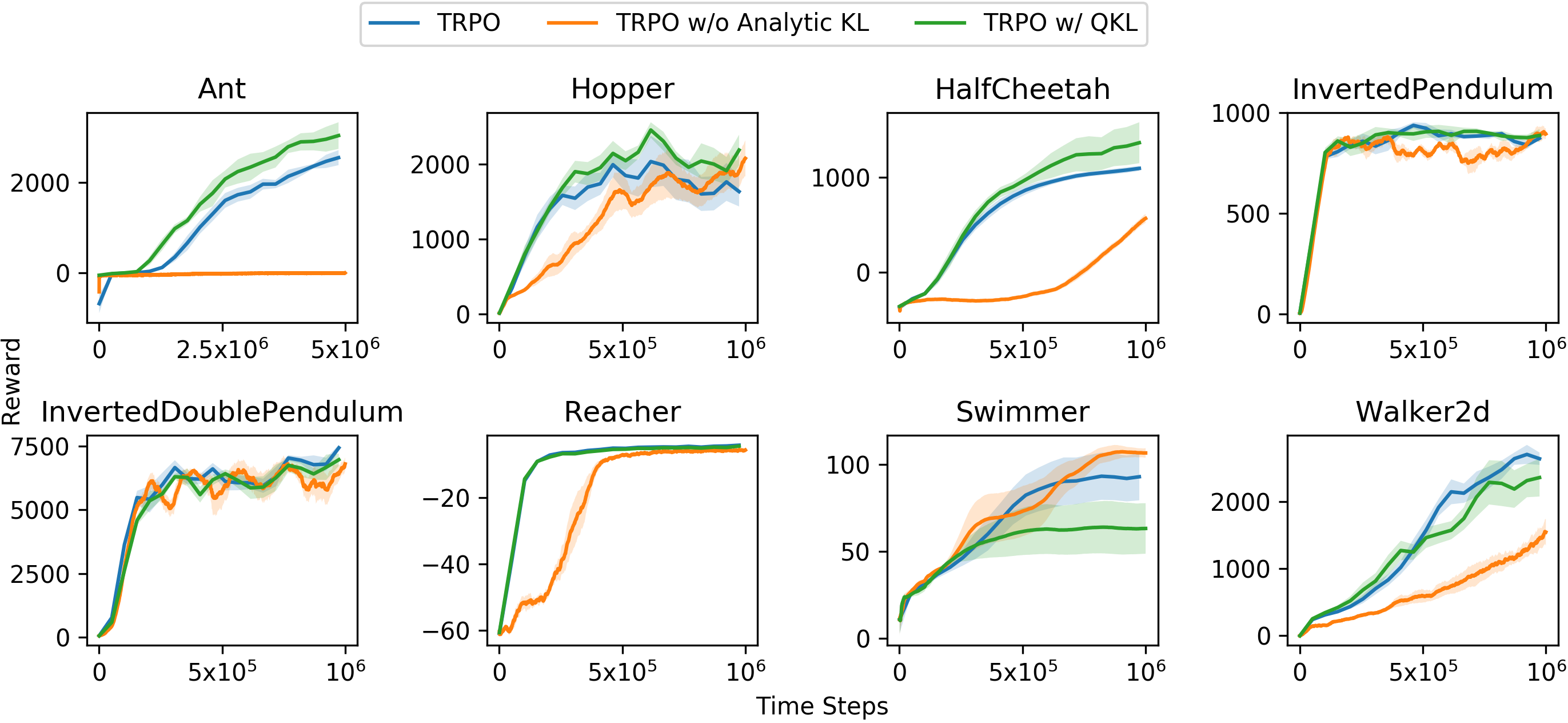
Refer to caption
Figure 8: Reward of QKL-TRPO (TRPO w/ QKL), TRPO without analytical KL (TRPO w/o Analytic KL), and the original TRPO (TRPO) in several MuJoCo benchmarks.

We test QKL-TRPO compared with the original TRPO in several MuJoCo benchmarks. We follow the same hyperparameters recommended in OpenAI Baseline. The only difference between these two versions of TRPOs is the method utilized to estimate KL divergence between old and new policies. From the results, we can see that QKL-TRPO performs better in (Ant, HalfCheetah, Hopper), comparable in (InvertedDoublePendulum, InvertedPendulum, Reacher), while worse in (Swimmer, Walker2d). Note that the KL divergence expectation is estimated by 𝔼sρθ~(s)[DKL(πθ~||πθ)]\mathop{\mathbb{E}}_{s\sim\rho_{\tilde{\theta}}(s)}\left[D_{KL}(\pi_{\tilde{\theta}}||\pi_{\theta})\right] with the analytical form of KL divergence over all collected s𝑠s for the original TRPO while 𝔼s,a[0.5(logπθ~logπθ)2]subscript𝔼𝑠𝑎delimited-[]0.5superscriptsubscript𝜋~𝜃subscript𝜋𝜃2\mathop{\mathbb{E}}_{s,a}\left[0.5(\log\pi_{\tilde{\theta}}-\log\pi_{\theta})^{2}\right] over all (s,a)𝑠𝑎(s,a) pairs for QKL-TRPO. The latter (s,a)𝑠𝑎(s,a)-based estimation method should have caused a much higher variance, resulting in lower performance (TRPO w/o Analytic KL in Figure 8). However, thanks to QKL, QKL-TRPO achieves comparable performance with TRPO.

G.2 Ablation Study

We have conducted a series of ablation study to investigate the impacts of main components of HTRPO, Quadratic KL divergence estimation (QKL) and hindsight goal filtering (HGF), as well as the weighted importance sampling (WIS). Besides, we also provide a comprehensive comparison between dense-reward and sparse-reward HTRPO. All results are shown in Figure 9.
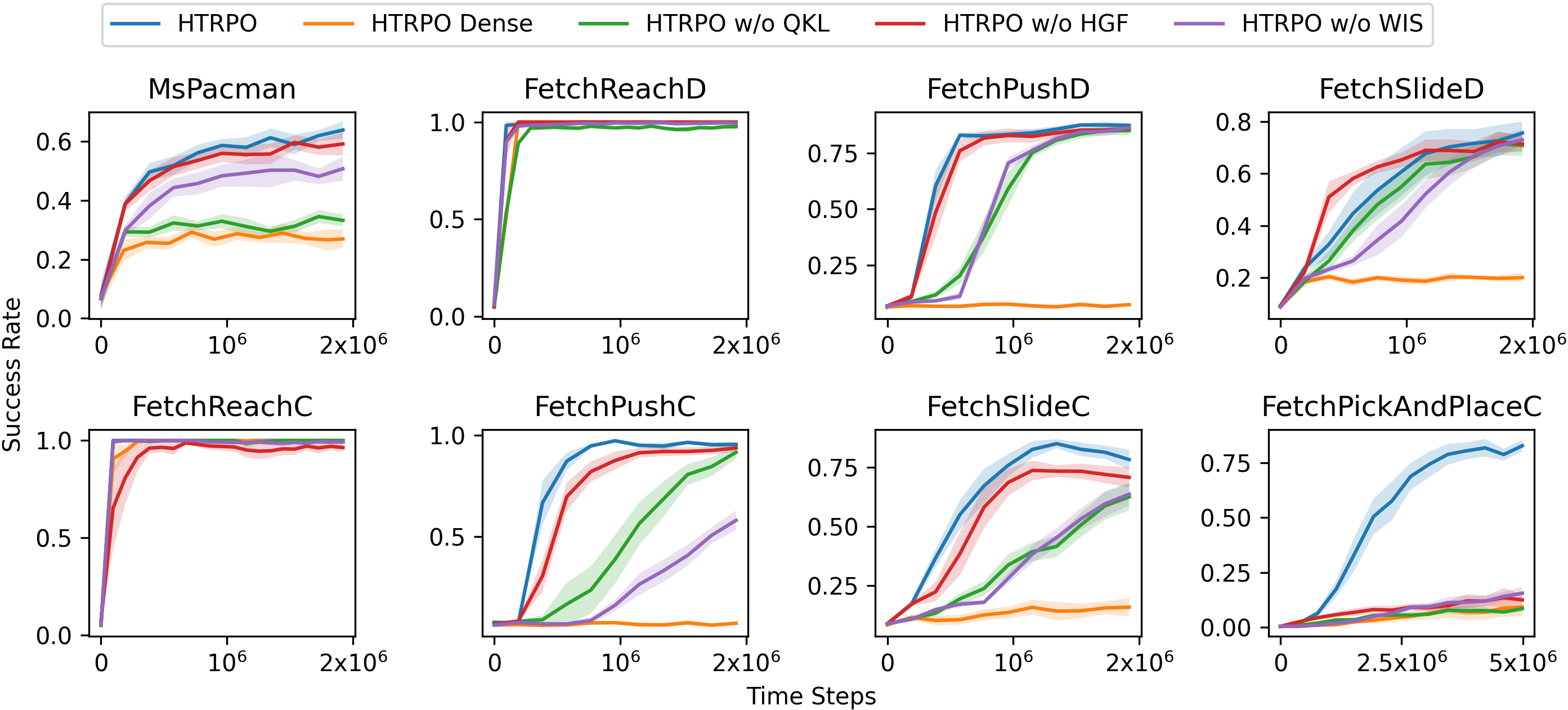
Refer to caption
Figure 9: Ablation study of HTRPO.
Quadratic KL divergence Estimation:

QKL is a main component of HTRPO, which imposes a reliable trust region constraint for finding a local optimum. As is known, the vanilla KL estimation suffers from high variance and fails to give an accurate estimation, which leads to instability during learning. It accords with the results that “HTRPO w/o QKL” performs much worse than “HTRPO” in both converging speed and final success rate.
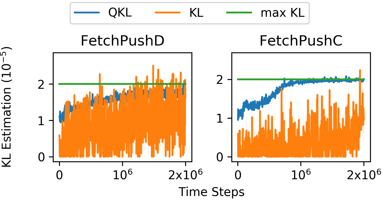
Refer to caption
Figure 10: Variance of different KL estimation methods.

To illustrate the advantage of QKL more intuitively, Figure 10 provides the curves of KL estimation during the learning process for Discrete Fetch Push and Continuous Fetch PickAndPlace as examples. As known, the line search method in TRPO helps enhance learning stability. However, due to the high variance of vanilla KL estimation, when encountering an overestimated result, line search imposes a smaller update step. Such regulation underestimates the range of trust region and therefore, the vanilla KL estimation is randomly much lower than the expected KL(noted as max KL step). It introduces unstable update by finding the local optima in inappropriate trust regions. In comparison, the low variance of QKL ensures a comparatively accurate estimation and better accords with the max KL step. Still, in Figure 10, the KL curve of HTRPO is slightly below the max KL step, because we adopt a conjugate-gradient damping coefficient to enhance the training stability as in Schulman et al. [2015a].

Hindsight Goal Filtering:

HGF scatters hindsight goals over the original goal space, which better guides the agent to successfully reach every possible original goal. To verify the contribution of HGF, we ablate this hindsight goal selecting method and provide the corresponding performance in Figure 9. As demonstrated, the algorithm would suffer a decrease in success rate more or less without HGF. Such degradation of performance becomes severe in complex tasks like Fetch PickAndPlace. Given that original goals mainly distribute in the air versus that most hindsight goals remain initially on the table, such discrepancy impedes the agent’s progress of learning to reach the original goals. With the assistance of HGF, the selected hindsight goals cover the original goal space as much as possible, which, to a great extent, guarantees the successful reach to goals from the original goal space once the agent has learned to reach goals from the hindsight goal space. Hence, a good hindsight goal selection method brings significant benefit for hindsight data driven learning approaches.

Weighted Importance Sampling:

Weighted importance sampling is utilized for variance reduction of importance sampling bishop2016pattern. In the experiment, we compare HTRPO with “HTRPO without WIS”. Admittedly, we can see that the performance of “HTRPO without WIS” matches the full version of HTRPO in some simple tasks such as Continuous Fetch Reach. However, for more complex ones like Fetch Push and Fetch Slide, the variance is detrimentally larger than that in simple tasks. And we can see as the environment get more complex, the benefits of weighted importance sampling significantly improves the performance. In short, the performance of “HTRPO without WIS” has a severe degradation comparing to the full version of HTRPO.

To further demonstrate the sampling efficiency, we also follow a well-known method ESS^=1/w¯2^𝐸𝑆𝑆1superscript¯𝑤2\widehat{ESS}=1/\sum\overline{w}^{2}, where w¯¯𝑤\overline{w} is the normalized importance weight, to estimate the effective sample sizes (ESS) of the importance weights by taking FetchPushC as an example. During learning, since we do have 3.2k time steps in each batch, by sampling 100 hindsight goals, there are about 320k importance-weighted samples. The corresponding ESS is 11.6k on average during the learning. It is also interesting that the ESS will decrease as the training progresses since the entropy of the policy will decrease.