An exact penalty approach for optimization with nonnegative orthogonality constraints

Abstract

Optimization with nonnegative orthogonality constraints has wide applications in machine learning and data sciences. It is NP-hard due to some combinatorial properties of the constraints. We first propose an equivalent optimization formulation with nonnegative and multiple spherical constraints and an additional single nonlinear constraint. Various constraint qualifications, the first- and second-order optimality conditions of the equivalent formulation are discussed. By establishing a local error bound of the feasible set, we design a class of (smooth) exact penalty models via keeping the nonnegative and multiple spherical constraints. The penalty models are exact if the penalty parameter is sufficiently large other than going to infinity. A practical penalty algorithm with postprocessing is then developed. It uses a second-order method to approximately solve a series of subproblems with nonnegative and multiple spherical constraints. We study the asymptotic convergence of the penalty algorithm and establish that any limit point is a weakly stationary point of the original problem and becomes a stationary point under some additional mild conditions. Extensive numerical results on the projection problem, orthogonal nonnegative matrix factorization problems and the K-indicators model show the effectiveness of our proposed approach.

65K05, 90C30, 90C46, 90C90

1 Introduction

In this paper, we consider optimization with nonnegative orthogonality constraints:

(1.1) $$\min_{X\in\mathbb{R}^{n\times k}}\,f(X)\quad\mathrm{s.t.}\quad X^{\top}X=I_{k},\ X\geq 0,$$

where $1\leq k\leq n$, $I_{k}$ is the $k$-by-$k$ identity matrix and $f\colon\mathbb{R}^{n\times k}\rightarrow\mathbb{R}$ is continuously differentiable. The feasible set of (1.1) is denoted as $\mathcal{S}^{n,k}_{+}\coloneqq\mathcal{S}^{n,k}\cap\mathbb{R}_{+}^{n\times k}$, where $\mathcal{S}^{n,k}\coloneqq\{X\in\mathbb{R}^{n\times k}:X^{\top}X=I_{k}\}$ is the Stiefel manifold. The non-negativity in $\mathcal{S}^{n,k}_{+}$ destroys the smoothness of $\mathcal{S}^{n,k}$ and introduces some combinatorial features. Specifically, a matrix $X\in\mathcal{S}^{n,k}_{+}$ means that each row of $X$ has at most one positive element and each column of $X$ takes the unit norm. Problem (1.1) has captured a wide variety of applications and interests, see [8, 7, 32, 52, 58] and the references therein.

Due to the combinatorial features, solving (1.1) is generally NP-hard. Actually, problem (1.1) covers some classical NP-hard problems, such as the problem of checking copositivity of a symmetric matrix [24], the quadratic assignment problem and the more general optimization over permutation matrices [27] as special cases. Besides, the constraint $X\in\mathcal{S}^{n,k}_{+}$ also appears in the $k$-means clustering [14, 17], the min-cut problem [42], etc. Several typical instances of problem (1.1) are briefly reviewed as follows.

1.1 Applications

We mainly introduced three classes of problem (1.1). The first one is the so-called trace minimization with nonnegative orthogonality constraints, formulated as

(1.2) $$\min_{X\in\mathcal{S}^{n,k}_{+}}\,\mathrm{tr}(X^{\top}MX),$$

where $M\in\mathbb{R}^{n\times n}$ is symmetric. If $M=-AA^{\top}$ with $A\in\mathbb{R}^{n\times r}$ being some data matrix, (1.2) is known as nonnegative principal component analysis [38, 56]. If $M=D-W$ with $W$ being a similarity matrix corresponding to $n$ objects and $D$ is a diagonal matrix having the same main diagonal as $W\mathbf{e}$, where $\mathbf{e}$ is the all-one vector, (1.2) is known as the nonnegative Laplacian embedding [33]. If $M=D-W+\mu R$ with some particularly chosen matrix $R$ and nonnegative regularization parameter $\mu$, (1.2) is known as the discriminative nonnegative spectral clustering [53].

The second one is the orthogonal nonnegative matrix factorization (ONMF) [21]. Given the data matrix $A\in\mathbb{R}_{+}^{n\times r}$, ONMF solves

(1.3) $$\min_{X\in\mathcal{S}^{n,k}_{+},Y\in\mathbb{R}_{+}^{r\times k}}\,\|A-XY^{\top}\|_{\mathtt{F}}^{2}.$$

Based on the idea of approximating the data matrix $A$ by its nonnegative subspace projection, Yang and Oja [54] proposed the orthonormal projective nonnegative matrix factorization (OPNMF) model as follows:

(1.4) $$\min_{X\in\mathcal{S}^{n,k}_{+}}\,\|A-XX^{\top}A\|_{\mathtt{F}}^{2}.$$

Models (1.3) and (1.4) are equivalent since the optimal solutions $\bar{X}$ and $\bar{Y}$ of (1.3) satisfy the relation $\bar{Y}=A^{\top}\bar{X}$. Yang and Oja [54] also proposed a special OPNMF model by replacing the Frobenius norm in (1.4) by the Kullback-Leibler divergence of $A$ and $XX^{\top}A$. The orthogonal symmetric non-negative matrix factorization models were considered in [29, 40].

The third one is an efficient K-indicators model for data clustering proposed by Chen et al. [19]. Let $U\in\mathcal{S}^{n,k}$ be the features matrix extracted from the data matrix $A\in\mathbb{R}^{n\times r}$, the K-indicators model in [19] reads

(1.5) $$\min_{X\in\mathcal{S}^{n,k}_{+},Y\in\mathcal{S}^{k,k}}\,\|UY-X\|_{\mathtt{F}}^{2}\quad\mathrm{s.t.}\quad\|X_{i,:}\|_{0}=1,i\in[n],$$

where $\|X_{i,:}\|_{0}$ is the number of nonzero elements in the $i$-th row of $X$, namely, $X_{i,:}$.

1.2 Related works

Optimization on the Stiefel manifold [1, 47] has already been well explored. However, a systematic study on problem (1.1) is lacked in the literature albeit it captures many applications. The existing works rarely considered the general problem (1.1), and most of them focused on some special formulations of (1.1). We briefly review some main existing methods. For solving ONMF model (1.3), motivated by the multiplicative update methods for nonnegative matrix factorization, Ding et al. [21] and Yoo and Choi [55] gave two different multiplicative update schemes. By establishing the equivalence of ONMF with a weighted variant of spherical $k$-means, Pompoli et al. [41] proposed an EM-like algorithm. Pompoli et al. [41] also designed an augmented Lagrangian method via penalizing the nonnegative constraints but keeping the orthogonality constraints. Li et al. [30] and Wang et al. [45, 46] considered the nonconvex penalty approach by keeping the nonnegative constraints. Some theoretical properties of the nonconvex penalty model were investigated in [46] but the results may not be applied directly to the general problem (1.1). Zhang et al. [59] proposed a greedy orthogonal pivoting algorithm which can promote exact orthogonality. For solving OPNMF model (1.4), Yang and Oja [54] designed a specific multiplicative update method. Pan and Ng [39] introduced a convex relaxation model, wherein the relaxed model is solved by the alternating direction method of multipliers. We remark that the multiplicative update scheme for solving problem (1.3) or (1.4) highly depends on the specific formulation of the objective function, so it is not easy to extend this class of methods to solve the general problem (1.1). In addition, Wen and Yin [47] designed an augmented Lagrangian method by penalizing the nonnegative constraints but keeping the orthogonality constraints for solving the quadratic assignment problem. Chen et al. [19] proposed a semi-convex relaxation model and construct a double-layered alternating projection scheme to solve the K-indicators model (1.5).

1.3 Our contribution

By well exploring the structure of $\mathcal{S}^{n,k}_{+}$, we first give a new characterization of $\mathcal{S}^{n,k}_{+}$ as

(1.6) $$\mathcal{S}^{n,k}_{+}=\mathcal{X}_{V}\coloneqq\mathcal{OB}^{n,k}_{+}\cap\{X\in\mathbb{R}^{n\times k}:\|XV\|_{\mathtt{F}}=1\},$$

where $\mathcal{OB}^{n,k}_{+}=\{X\in\mathbb{R}^{n\times k}:\|\mathbf{x}_{j}\|=1,\mathbf{x}_{j}\geq 0,j\in[k]\}$, in which $\mathbf{x}_{j}$ denotes the $j$-th column of $X$, and the constant matrix $V\in\mathbb{R}^{k\times r}$($1\leq r\leq k$) satisfies $\|V\|_{\mathtt{F}}=1$ and $\min_{i,j\in[k]}[VV^{\top}]_{ij}>0$. Based on this equivalent characterization, a reformulation of problem (1.1) is given as

(1.7) $$\min_{X\in\mathcal{OB}^{n,k}_{+}}\,f(X)\quad\ \mathrm{s.t.}\quad\|XV\|_{\mathtt{F}}=1.$$

We show that the classical constraint qualifications (CQs) including cone-continuity property (CCP) and Abadie CQ (ACQ) only hold when $\|X\|_{0}=n$ while the weakest Guignard CQ (GCQ) always holds. The first- and second-order optimality conditions are also given for problem (1.7). We then explore the relationship between problems (1.1) and (1.7) and show that the two formulations not only share the same minimizers but also the same optimality conditions.

To motivate the exact penalty approach, we prove that a local error bound with exponent $1/2$ holds for $\mathcal{S}^{n,k}_{+}$. Therefore, via keeping the simple constraints $\mathcal{OB}^{n,k}_{+}$ and penalizing the constraint $\|XV\|_{\mathtt{F}}=1$, we propose a class of exact penalty models:

(1.8) $$\min_{X\in\mathcal{OB}^{n,k}_{+}}\,\left\{P_{\sigma,p,q,\epsilon}(X):=f(X)+\sigma\left(\zeta_{q}(X)+\epsilon\right)^{p}\right\},$$

where $\zeta_{q}(X):=\|XV\|_{\mathtt{F}}^{q}-1$, $\sigma>0$ is the penalty parameter and $p,q>0$ and $\epsilon\geq 0$ are the model parameters. An important feature of (1.8) is that it allows smooth penalty by choosing appropriate model parameters, such as choosing $p\geq 1$ and $\epsilon=0$. We show that if the penalty parameter $\sigma$ is chosen to be larger than a positive constant, the optimal solution of the exact penalty problem (possibly a postprocessing will be invoked) is also optimal for the original problem. A more general exact penalty model (3.9) is also discussed. Then we develop a practical exact penalty algorithm which approximately solves a series of penalty subproblems of the form (1.8) and performs a postprocessing procedure to further improve the solution quality. We study the asymptotic convergence of the penalty algorithm and show that any limit point of the sequence generated by the algorithm is a weakly stationary point of (1.7). We also provide some mild conditions under which the limit point is a stationary point of (1.7). To solve the subproblem (1.8) efficiently, we develop a second-order algorithm for solving optimization over $\mathcal{OB}^{n,k}_{+}$, which is of independent interest. We also discuss how to use the proposed penalty algorithmic framework to solve a two block model

(1.9) $$\min_{X\in\mathcal{S}^{n,k}_{+},Y\in\mathcal{Y}}\,f(X,Y),$$

where $\mathcal{Y}$ is some simple closed set such that the projection to the set $\mathcal{Y}$ is easy to compute. Finally, numerical results on the projection problem and ONMF on synthetic data, text clustering, hyperspectral unmixing and K-indicators model demonstrate the efficiency of our approach.

1.4 Organization

The rest of this paper is organized as follows. A new characterization of $\mathcal{S}^{n,k}_{+}$ and the equivalent reformulation of problem (1.1) are given in Section 2. We propose the exact penalty model in Section 3. A practical penalty algorithm together with its convergence results is presented in Section 4. We investigate a second-order method for solving the penalty subproblem, namely, optimization over $\mathcal{OB}^{n,k}_{+}$ in Section 5. A variety of numerical results are presented in Section 6. Finally, we make some concluding remarks in Section 7.

1.5 Notations

For a positive integer $n$, we denote $[n]\coloneqq\{1,\ldots,n\}$. The $j$-th column (resp. $i$-th row) of a matrix $Z$ with appropriate dimension is denoted by $Z_{:,j}$ (resp. $Z_{i,:}$). For simplicity, we also denote $\mathbf{z}_{j}\coloneqq Z_{:,j}$. Let $\mathcal{S}$ be a closed set, we use $\Pi_{\mathcal{S}}(\cdot)$ to denote the projection operator. The number of nonzero elements of $Z$ is $\|Z\|_{0}$. The Frobenius norm of $Z$ is $\|Z\|_{\mathtt{F}}$ while the 2-norm of a vector $z$ is $\|z\|$. For $z\in\mathbb{R}^{n}$, $\mathsf{Diag}(z)\in\mathbb{R}^{n\times n}$ is a diagonal matrix with the main diagonal being $z$. For $Z\in\mathbb{R}^{n\times n}$, $\mathsf{diag}(Z)\in\mathbb{R}^{n}$ is the main diagonal of $Z$. For simplicity, we use $\mathsf{Diag}(Z)$ to denote $\mathsf{Diag}(\mathsf{diag}(Z))$. Let $\mathsf{Of\;\!\!f}(Z)=Z-\mathsf{Diag}(Z)$. The inner product between two matrices $A$ and $B$ with the same sizes is $\langle A,B\rangle=\mathrm{tr}(A^{\top}B)$. The notation $0\leq A\perp B\geq 0$ means that $A\geq 0$ and $B\geq 0$ component-wisely and $A\circ B=0$, where $\circ$ means the Hadamard product operation. Similarly, $\min(A,B)$ takes the minimum of matrices $A$ and $B$ component-wisely.

2 Reformulation of problem (1.1)

Let $f^{*}$ and $\mathcal{X}^{*}$ be the optimal value and optimal solution set of problem (1.1) or (1.7), respectively. We define $\mathsf{sgn}(\mathcal{S}^{n,k}_{+}):=\{H\in\{0,1\}^{n,k}:H=\mathsf{sgn}(X)\ \mbox{with}\ X\in\mathcal{S}^{n,k}_{+}\}$, where $\mathsf{sgn}(X)_{ij}=|X_{ij}|/X_{ij}$ if $X_{ij}\neq 0$ and $\mathsf{sgn}(X)_{ij}=0$ otherwise. The set $\mathsf{sgn}(\mathcal{X}^{*})$ is defined accordingly. For ease of reference, we state a blanket assumption on problem (1.1) or (1.7).

Assumption 2.1.

We assume that $\emptyset\neq\mathsf{sgn}(\mathcal{S}^{n,k}_{+})\setminus\mathsf{sgn}(\mathcal{X}^{*}):=\{H\in\{0,1\}^{n,k}:H\in\mathsf{sgn}(\mathcal{S}^{n,k}_{+})\ \mbox{but}\ H\not\in\mathsf{sgn}(\mathcal{X}^{*})\}$, namely, the constant $\chi_{f}:=\tilde{f}^{*}-f^{*}>0$ with

$$\tilde{f}^{*}=\min_{X\in\mathbb{R}^{n\times k}}\,f(X)\quad\mathrm{s.t.}\quad X\in\mathcal{S}^{n,k}_{+},\mathsf{sgn}(X)\in\mathsf{sgn}(\mathcal{S}^{n,k}_{+})\setminus\mathsf{sgn}(\mathcal{X}^{*}).$$

If 2.1 does not hold, then $\mathsf{sgn}(\mathcal{S}^{n,k}_{+})\setminus\mathsf{sgn}(\mathcal{X}^{*})=\emptyset$, which with $\mathsf{sgn}(\mathcal{X}^{*})\subseteq\mathsf{sgn}(\mathcal{S}^{n,k}_{+})$ tells $\mathsf{sgn}(\mathcal{S}^{n,k}_{+})=\mathsf{sgn}(\mathcal{X}^{*})$. In this case, problem (1.1) or (1.7) is trivial in the sense that any $X$ with $\|X\|_{0}=k$ and having a $k$-by-$k$ permutation matrix as its submatrix is a global minimizer. However, we can verify that 2.1 holds for the test problems in section 6 by randomly choosing some matrices in $\mathcal{S}^{n,k}_{+}$ with different sign matrices and comparing their function values.

For $X\in\mathcal{S}^{n,k}_{+}$, we define $\mathsf{supp}(X):=\{(i,j)\in[n]\times[k]:X_{ij}\neq 0\}$ and $\Omega_{0}(X)=\left\{(i,j)\in[n]\times[k]:X_{ij}=0\right\}$. The set $\Omega_{0}(X)$ is splited into two disjoint sets as $\Omega^{\prime}_{0}(X)$$=\left\{(i,j)\in\Omega_{0}(X):\|X_{i,:}\|>0\right\}$ and $\Omega^{\prime\prime}_{0}(X)=\left\{(i,j)\in\Omega_{0}(X):\|X_{i,:}\|=0\right\}$.

We first give an equivalent algebraic characterization of $\mathcal{S}^{n,k}_{+}$.

Lemma.

For any $X\in\mathcal{OB}^{n,k}_{+}$, there holds that $\|XV\|_{\mathtt{F}}\geq 1$, where the equality holds if and only if $X\in\mathcal{S}^{n,k}_{+}$. Furthermore, the characterization (1.6) holds.

Proof.

With $\|V\|_{\mathtt{F}}=1$ and $X\in\mathcal{OB}^{n,k}_{+}$, we have $\|XV\|_{\mathtt{F}}^{2}-1=\left\langle VV^{\top},X^{\top}X-I_{p}\right\rangle$ $=\sum_{i,j\in[k],i\neq j}[VV^{\top}]_{ij}(\mathbf{x}_{i}^{\top}\mathbf{x}_{j}),$ which with $VV^{\top}>0$ implies that $\|XV\|_{\mathtt{F}}^{2}-1\geq 0$. The equality holds if and only if $\mathbf{x}_{i}^{\top}\mathbf{x}_{j}=0$ for $i,j\in[k]$ and $i\neq j$, which with $X\in\mathcal{OB}^{n,k}_{+}$ means that $X\in\mathcal{S}^{n,k}_{+}$. Hence (1.6) follows directly. The proof is completed.

With the equivalent characterization (1.6) of $\mathcal{S}^{n,k}_{+}$ and Lemma Lemma, we reformulate problem (1.1) as problem (1.7). Throughout this paper, we mainly focus on the formulation (1.7) since it gives us more insight to design our exact penalty approach. We are now going to discuss the CQs and first- and second-order optimality conditions (1.7) and investigate the relationship between the two formulations (1.1) and (1.7).

2.1 Constraint qualifications of problem (1.7)

In this subsection, we investigate several CQs of problem (1.7) which are important to establish the optimality conditions. We mainly consider, Guignard CQ (GCQ), which is the weakest CQ, Abadie CQ (ACQ) and the cone-continuity property (CCP), which is the weakest strict CQ [2]. Note that the following implications hold: CCP $\Longrightarrow$ ACQ $\Longrightarrow$ GCQ.

We first give the expression of the tangent cone $\mathcal{T}_{\mathcal{X}_{V}}(X)$ and linearized cone $\mathcal{L}_{\mathcal{X}_{V}}(X)$ at $X\in\mathcal{X}_{V}$. Following the definition of linearized cone, we have

(2.1) $$\mathcal{L}_{\mathcal{X}_{V}}(X)=\left\{D\in\mathbb{R}^{n\times k}:\begin{array}[]{l}\mathbf{x}_{j}^{\top}\mathbf{d}_{j}=0\ \forall j\in[k],\\ D_{ij}\geq 0\ \forall(i,j)\in\Omega_{0}(X),\langle D,XVV^{\top}\rangle=0\end{array}\right\}.$$

With the choice of $V$ and (1.6), $\langle D,XVV^{\top}\rangle$ $=0$ tells that $\mathbf{d}_{i}^{\top}\sum_{j\in[k]}(VV^{\top})_{ji}\mathbf{x}_{j}=0$ which further implies that $D_{ij}=0$ if $(i,j)\in\Omega_{0}^{\prime}(X)$. This together with the definitions of $\Omega_{0}^{\prime}(X)$ and $\Omega_{0}^{\prime\prime}(X)$ and (2.1) yields

(2.2) $$\mathcal{L}_{\mathcal{X}_{V}}(X):={}\left\{D\in\mathbb{R}^{n\times k}:\!\!\!\!\!\!\!\begin{array}[]{ll}&\mathbf{x}_{j}^{\top}\mathbf{d}_{j}=0\ \forall j\in[k],D_{ij}=0\ \forall(i,j)\in\Omega_{0}^{\prime}(X),\\ &D_{ij}\geq 0\ \forall(i,j)\in\Omega_{0}^{\prime\prime}(X)\end{array}\!\!\right\}.$$

The tangent cone at $X$ is given as $\mathcal{T}_{\mathcal{X}_{V}}(X)=\{D\in\mathbb{R}^{n\times k}:\exists\alpha^{l}>0,\alpha^{l}\rightarrow 0,D^{l}\rightarrow D\ \mbox{such that}\ X^{l}:=\bar{X}+\alpha^{l}D^{l}\in\mathcal{X}_{V}\}$. Clearly we have $\mathcal{T}_{\mathcal{X}_{V}}(X)\subseteq\mathcal{L}(X)$. For each $l$ and $i\in[n]$, there is at most one element of $(X^{l}-X)_{ij}\ \forall(i,j)\in\Omega_{0}^{\prime\prime}(X)$ being nonzero. Hence, any $D\in\mathcal{T}_{\mathcal{X}_{V}}(X)$ must satisfy $\|D_{i,:}\|_{0}\leq 1$ if $X_{i,:}=0$. On the other hand, for any $D\in\mathcal{L}_{\mathcal{X}_{V}}(X)$ with $\|D_{i,:}\|_{0}\leq 1$ if $X_{i,:}=0$, choosing $D^{l}\equiv D$, $\alpha^{l}=1/l$ and $X^{l}$ as $\mathbf{x}_{j}^{l}=(\mathbf{x}_{j}+\alpha^{l}\mathbf{d}_{j})/\|\mathbf{x}_{j}+\alpha^{l}\mathbf{d}_{j}\|$, it is clear that $X^{l}\in\mathcal{X}_{V}$. This means that $D\in\mathcal{T}_{\mathcal{X}_{V}}(X)$. In summary, we arrive at

(2.3) $$\mathcal{T}_{\mathcal{X}_{V}}(X)=\mathcal{L}_{\mathcal{X}_{V}}(X)\cap\left\{D\in\mathbb{R}^{n\times k}:\|D_{i,:}\|_{0}\leq 1\ \mathrm{if}\ X_{i,:}=0\ \forall i\in[n]\right\}.$$

We now discuss the CQs in the following lemma.

Lemma.

Consider a feasible $\bar{X}\in\mathcal{X}_{V}$ of (1.7). If $k=1$, then the linear independence constraint qualification (LICQ) holds at $\bar{X}$; if $2\leq k\leq n$ and $\|\bar{X}\|_{0}=n$, then CCP holds; if $2\leq k\leq n$ and $\|\bar{X}\|_{0}<n$, then GCQ holds but ACQ fails to hold.

Proof.

Case I. $k=1$. It is straightforward to check that LICQ holds at $\bar{X}$.

Case II. $2\leq k\leq n$ and $\|\bar{X}\|_{0}=n$, namely, each row of $\bar{X}$ has exactly one positive element. In this case $\Omega^{\prime}_{0}(\bar{X})=\Omega_{0}(\bar{X})$ and $\Omega^{\prime\prime}_{0}(\bar{X})=\emptyset$. For a sequence $\{X^{l}\}\subset\mathcal{X}_{V}$ and $X^{l}\rightarrow\bar{X}$, we consider the closed convex cone, which is related to CCP, as

$$\mathcal{K}_{\mathcal{X}_{V}}(X^{l})=\left\{X^{l}\mathsf{Diag}(\Lambda)+\lambda X^{l}VV^{\top}-\sum_{(i,j)\in\Omega_{0}(\bar{X})}Z_{ij}\mathbf{E}_{ij}:\Lambda\in\mathbb{R}^{k},\lambda\in\mathbb{R},Z_{ij}\in\mathbb{R}_{+}\right\}$$

where $\mathbf{E}_{ij}\in\mathbb{R}^{n\times k}$ with $(i,j)$ element being one while the remaining elements being zeros. Since $\mathcal{X}_{V}\owns X^{l}\rightarrow\bar{X}$ and $\Omega_{0}^{\prime\prime}(\bar{X})=\emptyset$, we have $\Omega_{0}(X^{l})=\Omega(\bar{X})$ and $\mathsf{supp}(X^{l})=\mathsf{supp}(\bar{X})$ for sufficiently large $l$. Thus $X^{l}VV^{\top}=X^{l}\mathsf{Diag}(VV^{\top})+\sum_{(i,j)\in\Omega_{0}(\bar{X})}Z_{ij}\mathbf{E}_{ij}$ for some $Z_{ij}\in\mathbb{R}_{+}$. By some easy calculations, one have

(2.4) $$\mathcal{K}_{\mathcal{X}_{V}}(X^{l})=\left\{X^{l}\mathsf{Diag}(\Lambda)+\sum_{(i,j)\in\Omega_{0}(\bar{X})}Z_{ij}\mathbf{E}_{ij}:\Lambda\in\mathbb{R}^{k},Z_{ij}\in\mathbb{R}\right\}$$

for sufficiently large $l$, which with $X^{l}\rightarrow\bar{X}$ implies that $\limsup_{X^{l}\rightarrow\bar{X}}\mathcal{K}_{\mathcal{X}_{V}}(X^{l})\subset\mathcal{K}_{\mathcal{X}_{V}}(\bar{X})$. This means that CCP holds in this case.

Case III. $2\leq k\leq n$ and $\|\bar{X}\|_{0}<n$. In this case, $\Omega^{\prime\prime}_{0}(\bar{X})\neq\emptyset$. By definition, it is easy to verify that the polar cones of $\mathcal{T}(X)$ and $\mathcal{L}(X)$ coincide, namely,

$$\mathcal{T}_{\mathcal{X}_{V}}(X)^{\circ}=\mathcal{L}_{\mathcal{X}_{V}}(X)^{\circ}=\left\{D\in\mathbb{R}^{n\times k}:\begin{array}[]{ll}D_{ij}=\lambda_{j}X_{ij},\lambda_{j}\in\mathbb{R}\ \forall(i,j)\in\mathsf{supp}(X),\\ D_{ij}\leq 0\ \forall(i,j)\in\Omega^{\prime\prime}_{0}(X)\end{array}\right\}.$$

This means GCQ holds. Recalling $\Omega^{\prime\prime}_{0}(\bar{X})\neq\emptyset$, we know from (2.2) and (2.3) that $\mathcal{T}_{\mathcal{X}_{V}}(X)\subsetneq\mathcal{L}_{\mathcal{X}_{V}}(X)$, which tells that ACQ does not hold. The proof is completed.

2.2 Optimality conditions of problem (1.7)

Denote the Riemannian gradient [1] with respect to the oblique manifold $\mathcal{OB}^{n,k}$ as

(2.5) $$\mathrm{grad}\,f(X)=\nabla f(X)-X\mathsf{Diag}\big{(}X^{\top}\nabla f(X)\big{)}.$$

Theorem (First-order necessary conditions).

Suppose that $\bar{X}\in\mathcal{X}_{V}$ is a local minimizer of (1.7). Then $\bar{X}$ is a stationary point of (1.7), namely, $-\nabla f(\bar{X})\in\mathcal{L}_{\mathcal{X}_{V}}(\bar{X})^{\circ}$, which can be further represented as

(2.6a) $$[\mathrm{grad}\,f(\bar{X})]_{ij}=0\quad\forall(i,j)\in\mathsf{supp}(\bar{X}),$$

(2.6b) $$[\nabla f(\bar{X})]_{ij}\geq 0\quad\forall(i,j)\in\Omega^{\prime\prime}_{0}(\bar{X}).$$

Proof.

Lemma Lemma tells that GCQ holds at $\bar{X}$. Thus, $\bar{X}$ must be a stationary point and $-\nabla f(\bar{X})\in\mathcal{L}_{\mathcal{X}_{V}}(\bar{X})^{\circ}$ due to [9, Proposition 3.3.14]. Hence, there exists Lagrange multiplier vector $\bar{\Lambda}\in\mathbb{R}^{k}$ corresponding to $\|\mathbf{x}_{j}\|^{2}=1,j\in[k]$, Lagrange multiplier $\bar{\lambda}\in\mathbb{R}$ corresponding to $\|XV\|_{\mathtt{F}}=1$ and Lagrange multiplier matrix $\bar{Z}\in\mathbb{R}_{+}^{n\times k}$ corresponding to $X\geq 0$ such that $0\leq\bar{X}\perp\bar{Z}\geq 0$ and $\nabla_{X}L(\bar{X},\bar{\Lambda},\bar{Z},\bar{\lambda})=0$, namely,

(2.7) $$\nabla f(\bar{X})-\bar{X}\mathsf{Diag}\big{(}2\bar{\Lambda}-\bar{\lambda}\mathsf{diag}(VV^{\top})\big{)}-\bar{Z}+\bar{\lambda}\bar{X}\mathsf{Of\;\!\!f}(VV^{\top})=0.$$

Here, the Lagrangian function is given as

(2.8) $$L(X,\bar{\Lambda},Z,\bar{\lambda})=f(X)-\sum_{j\in[k]}\bar{\Lambda}_{j}(\|\mathbf{x}_{j}\|^{2}-1)-\left\langle\bar{Z},X\right\rangle+\bar{\lambda}(\|XV\|_{\mathtt{F}}-1).$$

Multiplying $\bar{X}^{\top}$ on both sides of (2.7) and then performing the $\mathsf{diag}(\cdot)$ operator, with $\bar{X}^{\top}\bar{X}=I_{k}$, we have $2\bar{\Lambda}-\bar{\lambda}\mathsf{diag}(VV^{\top})=\mathsf{diag}(\bar{X}^{\top}\nabla f(\bar{X})),$ which again with (2.7) and (2.5) implies that $\bar{Z}=\mathrm{grad}\,f(\bar{X})+\bar{\lambda}\bar{X}\mathsf{Of\;\!\!f}(VV^{\top})$. Recalling $\bar{X}\in\mathcal{X}_{V}$, it is easy to verify that $[\bar{X}\mathsf{Of\;\!\!f}(VV^{\top})]_{ij}=0$ $\ \forall(i,j)\in\mathsf{supp}(\bar{X})$, $[\bar{X}\mathsf{Of\;\!\!f}(VV^{\top})]_{ij}>0\ \forall(i,j)\in\Omega_{0}^{\prime}(\bar{X})$ and $[\mathrm{grad}\,f(\bar{X})]_{ij}$$=[\nabla f(\bar{X})]_{ij}\ \forall(i,j)\in\Omega^{\prime}_{0}(\bar{X})\cup\Omega^{\prime\prime}_{0}(\bar{X})$. Hence, we have

(2.9) $$\bar{Z}_{ij}=\begin{cases}[\mathrm{grad}\,f(\bar{X})]_{ij}&(i,j)\in\mathsf{supp}(\bar{X}),\\ [\nabla f(\bar{X})]_{ij}+\bar{\lambda}[\bar{X}\mathsf{Of\;\!\!f}(VV^{\top})]_{ij}&(i,j)\in\Omega^{\prime}_{0}(\bar{X}),\\ [\nabla f(\bar{X})]_{ij}&(i,j)\in\Omega^{\prime\prime}_{0}(\bar{X}).\end{cases}$$

For each $(i,j)\in\Omega^{\prime}_{0}(\bar{X})$, we can always choose

(2.10) $$\bar{\lambda}\geq\bar{\lambda}(\bar{X}):=\max_{(i.j)\in\Omega^{\prime}_{0}(\bar{X})}\frac{-[\nabla f(\bar{X})]_{ij}}{[\bar{X}\mathsf{Of\;\!\!f}(VV^{\top})]_{ij}}$$

such that $\bar{Z}_{ij}\geq 0$. Thus we arrive at the equivalent formulation (2.6a) and (2.6b).

We borrow the idea from mathematical programs with complementarity constraints, see [43] for instance, to define a weakly stationary point $\bar{X}$ of problem (1.7).

Definition.

We call $\bar{X}\in\mathcal{X}_{V}$ a weakly stationary point of problem (1.7) if (2.6a) holds at $\bar{X}$.

Note that a weakly stationary point $\bar{X}$ has no requirements on the sign of the Lagrange multiplier $[\nabla f(\bar{X})]_{ij}$ with $(i,j)\in\Omega_{0}^{\prime\prime}(\bar{X})$ and it is actually a stationary point of problem (1.7) with additional constraints $X_{ij}=0\ \forall(i,j)\in\Omega_{0}^{\prime\prime}(\bar{X})$. In the case when $\Omega_{0}^{\prime\prime}(\bar{X})=\emptyset$, namely, $\|\bar{X}\|_{0}=n$ or $\nabla f(\bar{X})\geq 0$ always holds, then the weakly stationary point $\bar{X}$ becomes a stationary point of problem (1.7).

We now assume that $f$ in problem (1.7) is twice continuously differentiable. The set of all sequential null constraint directions at a stationary point $\bar{X}$ (see Definition 8.3.1 in [44]) of problem (1.7) is given as

$$\mathcal{N}_{\mathcal{X}_{V}}(\bar{X},\bar{Z})=\left\{\!D\in\mathbb{R}^{n\times k}:\!\begin{array}[]{l}X^{l}:=\bar{X}+\alpha^{l}D^{l}\in\mathcal{X}_{V},\alpha^{l}>0,\alpha^{l}\rightarrow 0,D^{l}\rightarrow D,\\ X^{l}_{ij}=0\ \mbox{if}\ \bar{Z}_{ij}>0,X^{l}_{ij}\geq 0\ \mbox{if}\ \bar{Z}_{ij}=0\end{array}\!\right\}\!.$$

Notice that $\mathcal{N}_{\mathcal{X}_{V}}(\bar{X},\bar{Z})\subseteq\mathcal{T}_{\mathcal{X}_{V}}(\bar{X})$, with (2.9) and (2.3), we have

(2.11) $$\mathcal{N}_{\mathcal{X}_{V}}(\bar{X},\bar{Z})=\mathcal{T}_{\mathcal{X}_{V}}(\bar{X})\cap\left\{\!D\in\mathbb{R}^{n\times k}:D_{ij}=0\ \mbox{if}\ [\nabla f(\bar{X})]_{ij}>0\ \forall(i,j)\in\Omega^{\prime\prime}_{0}(\bar{X})\right\}\!.$$

Since $\mathcal{N}_{\mathcal{X}_{V}}$ is independent of $Z$, we write for $\mathcal{N}_{\mathcal{X}_{V}}(\bar{X},\bar{Z})$ as $\mathcal{N}_{\mathcal{X}_{V}}(\bar{X})$ for short. Similarly, we have the set of all linearized null constraint directions at $\bar{X}$, also known as the critical cone, $\mathcal{C}_{\mathcal{X}_{V}}(\bar{X})=\mathcal{L}_{\mathcal{X}_{V}}(\bar{X})\cap\{D\in\mathbb{R}^{n\times k}:D_{ij}=0\ \mbox{if}\ \bar{Z}_{ij}>0,(i,j)\in\Omega_{0}(\bar{X})\}$. Using (2.2), (2.9), (2.6a) and (2.6b), we further have

(2.12) $$\mathcal{C}_{\mathcal{X}_{V}}(\bar{X})=\mathcal{L}_{\mathcal{X}_{V}}(\bar{X})\cap\left\{D\in\mathbb{R}^{n\times k}:D_{ij}=0\ \mbox{if}\ [\nabla f(\bar{X})]_{ij}>0\ \forall(i,j)\in\Omega^{\prime\prime}_{0}(\bar{X})\right\}.$$

Define the Riemannian Hessian [1] with respect to the oblique manifold $\mathcal{OB}^{n,k}$ as

(2.13) $$\mathrm{Hess}\,f(X)[D]\coloneqq\nabla^{2}f(X)[D]-D\mathsf{Diag}\big{(}\bar{X}^{\top}\nabla f(X)\big{)},$$

where $D$ satisfies $\mathbf{x}_{j}^{\top}\mathbf{d}_{j}=0$ for $j\in[k]$. We are now ready to establish the second-order optimality conditions as follows.

Theorem (Second-order necessary conditions).

If $\bar{X}\in\mathcal{X}_{V}$ is a local minimizer of problem (1.7), then

(2.14) $$\left\langle D,\mathrm{Hess}\,f(\bar{X})[D]\right\rangle\geq 0,\quad\emph{for all}\ D\in\mathcal{N}_{\mathcal{X}_{V}}(\bar{X}).$$

Proof.

The proof of Theorem Theorem tells that $2\bar{\Lambda}-\bar{\lambda}\mathsf{diag}(VV^{\top})=\mathsf{diag}(\bar{X}^{\top}\nabla f(\bar{X}))$. With (2.8), we have $\nabla_{XX}^{2}L(\bar{X},\bar{\Lambda},\bar{Z},\bar{\lambda})[D]$ $=\mathrm{Hess}\,f(\bar{X})[D]+\bar{\lambda}D\mathsf{Of\;\!\!f}(VV^{\top})$. By [44, Theorem 8.3.3] and the fact that $\bar{X}$ is a local minimizer of problem (1.7), we have

(2.15) $$\left\langle D,\mathrm{Hess}\,f(\bar{X})[D]+\bar{\lambda}D\mathsf{Of\;\!\!f}(VV^{\top})\right\rangle\geq 0,\quad\mathrm{for\ all}\ D\in\mathcal{N}_{\mathcal{X}_{V}}(\bar{X}).$$

For $D\in\mathcal{N}_{\mathcal{X}_{V}}(\bar{X})$, we know from (2.11) that $D^{\top}D$ must be diagonal. Thus,

(2.16) $$\left\langle D,D\mathsf{Of\;\!\!f}(VV^{\top})\right\rangle=\mathrm{tr}(D^{\top}D\mathsf{Of\;\!\!f}(VV^{\top}))=0,$$

which with (2.15) implies (2.14). The proof is completed.

Theorem (Second-order sufficient conditions).

Suppose that $\bar{X}\in\mathcal{X}_{V}$ is a stationary point of problem (1.7) and that there exists a Lagrange multiplier $\bar{\lambda}$ associated to $\|XV\|_{\mathtt{F}}=1$ with $\bar{\lambda}\geq\bar{\lambda}(\bar{X})$ such that

(2.17) $$\left\langle D,\mathrm{Hess}\,f(\bar{X})[D]+\bar{\lambda}D\mathsf{Of\;\!\!f}(VV^{\top})\right\rangle>0,\quad\emph{for all}\ D\in\mathcal{C}_{\mathcal{X}_{V}}(\bar{X})/\{0\}.$$

Then $\bar{X}$ is a strict local minimizer of (1.7).

Proof.

It follows directly from, for instance [44, Theorems 8.3.4].

Remark.

Consider the case when $\Omega^{\prime\prime}_{0}(\bar{X})=\emptyset$, namely, $\|\bar{X}\|_{0}=n$. Following from (2.11), (2.12) and $\mathcal{T}_{\mathcal{X}_{V}}(\bar{X})=\mathcal{L}_{\mathcal{X}_{V}}(\bar{X})$, we have $\mathcal{N}_{\mathcal{X}_{V}}(\bar{X})=\mathcal{C}_{\mathcal{X}_{V}}(\bar{X})=\mathcal{L}_{\mathcal{X}_{V}}(\bar{X})$. Recalling (2.16), we thus know that (2.14) and (2.17) become $\left\langle D,\mathrm{Hess}\,f(\bar{X})[D]\right\rangle\geq 0$ $\forall D\in\mathcal{L}_{\mathcal{X}_{V}}(\bar{X})$ and $\left\langle D,\mathrm{Hess}\,f(\bar{X})[D]\right\rangle>0$ $\forall D\in\mathcal{L}_{\mathcal{X}_{V}}(\bar{X})/\{0\}$, respectively.

2.3 Relationship between problems (1.1) and (1.7)

It is clear that formulations (1.1) and (1.7) share the same minimizers. Moreover, the two problems share the same stationary points.

Lemma.

(i) The statements in Lemma Lemma hold for problem (1.1); (ii) Problems (1.1) and (1.7) share the same minimizers and optimality conditions.

Proof.

We first claim that that problems (1.1) and (1.7) have the same tangent and linearized cones. Obviously, we know $\mathcal{T}_{\mathcal{S}^{n,k}_{+}}(X)=\mathcal{T}_{\mathcal{X}_{V}}(X)$. For the linearized cone, we have $\mathcal{L}_{\mathcal{S}^{n,k}_{+}}(X)=\{D\in\mathbb{R}^{n\times k}:X^{\top}D+D^{\top}X=0,D_{ij}\geq 0\ \forall(i,j)\in\Omega_{0}(X)\}.$ The linear equation above tells that $\mathbf{x}_{l}^{\top}\mathbf{d}_{j}+\mathbf{d}_{l}^{\top}\mathbf{x}_{j}=0\ \forall l,j\in[n]$. With $X\in\mathcal{S}^{n,k}_{+}$ and $D_{ij}\geq 0\ \forall(i,j)\in\Omega_{0}(X)$, we further know that $\mathbf{x}_{l}^{\top}\mathbf{d}_{j}\geq 0$. Therefore, we have $\mathbf{x}_{l}^{\top}\mathbf{d}_{j}=0\ \forall l,j\in[n]$ and thus $\mathbf{x}_{j}^{\top}\mathbf{d}_{j}=0\ \forall j\in[n]$ and $D_{ij}=0\ \forall(i,j)\in\Omega_{0}^{\prime}(X)$. This means that $\mathcal{L}_{\mathcal{S}^{n,k}_{+}}(X)\subseteq\mathcal{L}_{\mathcal{X}_{V}}(X)$. On the other hand, it is easy to see that $D\in\mathcal{L}_{\mathcal{X}_{V}}(X)$ must imply that $D\in\mathcal{L}_{\mathcal{S}^{n,k}_{+}}(X)$. Hence, we have $\mathcal{L}_{\mathcal{S}^{n,k}_{+}}(X)=\mathcal{L}_{\mathcal{X}_{V}}(X)$. Besides, by some easy calculations, the cones $\mathcal{K}_{\mathcal{S}^{n,k}_{+}}(X)$ and $\mathcal{K}_{\mathcal{X}_{V}}(X)$ coincide, see (2.4) for the definition. This completes the proof of (i).

The proof of (ii) can be verified since $\mathcal{T}_{\mathcal{X}_{V}}(\bar{X})=\mathcal{T}_{\mathcal{S}^{n,k}_{+}}(\bar{X})$ and $\mathcal{N}_{\mathcal{S}^{n,k}_{+}}(\bar{X})=\mathcal{N}_{\mathcal{X}_{V}}(\bar{X})$ and $\mathcal{C}_{\mathcal{S}^{n,k}_{+}}(\bar{X})=\mathcal{C}_{\mathcal{X}_{V}}(\bar{X})$. The details are omitted to save space.

Based on the above lemma, it is safe to rewrite problem (1.1) as the equivalent problem (1.7). The reason that we prefer the latter one is that it can better motivate us to design the exact penalty approach. Simply speaking, we can afford to preserve the simpler constraints $\mathcal{OB}^{n,k}_{+}$ in our exact penalty algorithm but the nonnegative orthogonality constraint cannot be kept together in algorithms for (1.1). Moreover, only one simple constraint $\|XV\|_{\mathtt{F}}=1$ has to be penalized in our approach. This kind of framework is quite different from traditional exact penalty approaches applied to (1.1) directly.

3 An exact penalty approach

We now present the exact penalty properties. Let $X_{\sigma,p,q,\epsilon}$ be a global minimizer of (1.8) and denote $X^{\mathsf{R}}_{\sigma,p,q,\epsilon}$ as the matrix returned by Procedure 1 in Section 3.1 with an input $X_{\sigma,p,q,\epsilon}$. The solution quality can be further improved by solving an auxiliary problem constructed from $X^{\mathsf{R}}_{\sigma,p,q,\epsilon}$ as

(3.1) $$X^{\diamondsuit}_{\sigma,p,q,\epsilon}=\arg\min_{X\in\mathcal{OB}^{n,k}_{+}}f(X)\quad\mathrm{s.t.}\quad X_{ij}=0\ \mathrm{if}\ (i,j)\not\in\mathsf{supp}(X_{\sigma,p,q,\epsilon}^{\mathsf{R}}).$$

Let $L_{f}\geq 0$ be the Lipschitz constant of $f$, namely,

(3.2) $$|f(X_{1})-f(X_{2})|\leq L_{f}\|X_{1}-X_{2}\|_{\mathtt{F}},\quad\forall X_{1},X_{2}\in\mathcal{OB}^{n,k}_{+}.$$

Such $L_{f}$ exists since the convex hull of $\mathcal{OB}^{n,k}_{+}$ is compact. Let $\kappa_{f}=\chi_{f}/L_{f}$. We define

$$\underline{\nu}=\begin{cases}(\sqrt{2k})^{1-2p}&\mbox{if}\ 0<p\leq 1/2\ \mbox{and}\ \epsilon=0,\\[4.0pt] (\kappa_{f})^{1-2p}&\mbox{if}\ p>1/2\ \mbox{and}\ \epsilon=0,\\[4.0pt] \frac{\sqrt{2k}}{(\kappa_{f})^{2p}-(\varrho_{q}\sqrt{\epsilon})^{2p}}&\mbox{if}\ p>0\ \mbox{and}\ 0<\epsilon<\kappa_{f}^{2}/\varrho_{q}^{2},\end{cases}$$

where the constant $\varrho_{q}$ is defined later in Lemma Lemma.

The next theorem shows that if $\sigma$ is chosen sufficiently large, the optimal sign matrix can be obtained from $X^{\mathsf{R}}_{\sigma,p,q,\epsilon}$, thus $X^{\diamondsuit}_{\sigma,p,q,\epsilon}$ is also a solution of (1.7).

Theorem.

Under 2.1, if we choose

(3.3) $$\sigma>\underline{\sigma}:=\varrho_{q}^{2p}L_{f}\underline{\nu},$$

then it holds that (i) $\mathsf{sgn}(X_{\sigma,p,q,\epsilon}^{\mathsf{R}})\in\mathsf{sgn}(\mathcal{X}^{*})$; (ii) $X^{\diamondsuit}_{\sigma,p,q,\epsilon}$ is a global minimizer of problem (1.7).

We next investigate the error bound for $\mathcal{S}^{n,k}_{+}$ in section 3.1, then give the proof of Theorem Theorem for a class of general exact penalty model in section 3.2.

3.1 Error bound for $\mathcal{S}^{n,k}_{+}$

It is well known that the error bound plays a key role in establishing the exact penalty results, see [34] for more discussion. By [36, Theorem 16.7], we know that there exist positive scalars $\rho$ and $\gamma$ such that $\mathrm{dist}(X,\mathcal{S}^{n,k}_{+})=\|\Pi_{\mathcal{S}^{n,k}_{+}}(X)-X\|_{\mathtt{F}}\leq\rho(\zeta_{2}(X))^{\gamma},\forall X\in\mathcal{OB}^{n,k}_{+}$. However, the exponent $\gamma$ is not immediately clear for our case. We next show that the exponent is $\gamma=1/2$. Our key step is based on rounding Procedure 1. The basic idea for rounding is simply keeping one largest element in each row and setting the remaining elements to be zeros, and then doing normalization such that each column takes the unit norm.

Initialization: Set $H\in\mathbb{R}^{n\times k}$ as a zero matrix.

S1 For $i\in[n]$, set $H_{ij^{*}}=1\ \mbox{with}\ j^{*}\ \mbox{is the smallest index in the set}\mathop{\mathrm{argmax}}\nolimits_{j\in[k]}X_{ij}.$

S2 Set the $j$-th column of $X^{\mathsf{R}}$ as $\mathbf{x}^{\mathsf{R}}_{j}=\frac{\mathbf{x}_{j}\circ\mathbf{h}_{j}}{\|\mathbf{x}_{j}\circ\mathbf{h}_{j}\|},\ \ j\in[k].$

S3 Reset $X^{\mathsf{R}}=I_{n,k}$ if $X^{\mathsf{R}}\not\in\mathcal{S}^{n,k}_{+}$.

Algorithm 1 A procedure for rounding $X\in\mathcal{OB}^{n,k}_{+}$ to be $X^{\mathsf{R}}\in\mathcal{S}^{n,k}_{+}$.

Lemma.

For any $X\in\mathcal{OB}^{n,k}_{+}$, we have $X^{\mathsf{R}}\in\mathcal{S}^{n,k}_{+}$ and

(3.4) $$\mathrm{dist}(X,\mathcal{S}^{n,k}_{+})\leq\|X^{\mathsf{R}}-X\|_{\mathtt{F}}\leq\varrho_{q}\sqrt{\zeta_{q}(X)},$$

where $\varrho_{q}=\left({2k}\tilde{\varrho}_{q}/\underline{\omega}\right)^{\frac{1}{2}}$ with $\underline{\omega}={\min_{i,j\in[k]}[VV^{\top}]_{ij}}$. Here, $\tilde{\varrho}_{q}$ is 1 if $q\geq 2$, and is $\frac{\sqrt{k}+1}{q}$ if $1\leq q<2$, and is $\frac{2\sqrt{k}(\sqrt{k}+1)}{q(q+1)}$ if $0<q\leq 1$.

Proof.

We first focus on $q=2$. Recalling $\|V\|_{\mathtt{F}}=1$ and $\underline{\omega}>0$, we have

(3.5) $$\zeta_{2}(X)=\sum_{j\in[k]}\mathbf{x}_{j}^{\top}\Bigg{(}\sum_{l\in[k]\setminus\{j\}}(VV^{\top})_{jl}\mathbf{x}_{l}\Bigg{)}\geq\underline{\omega}\sum_{j\in[k]}\mathbf{x}_{j}^{\top}\Bigg{(}\sum_{l\in[k]\setminus\{j\}}\mathbf{x}_{l}\Bigg{)}.$$

The proof of (3.4) is split to two cases.

Case I. $\zeta_{2}(X)\geq\underline{\omega}$. Since $X^{\mathsf{R}}\in\mathcal{S}^{n,k}_{+}$ and $X\in\mathcal{OB}^{n,k}_{+}$, we obtain $\|X^{\mathsf{R}}\|_{\mathtt{F}}^{2}=\|X\|_{\mathtt{F}}^{2}=2k$ and thus $\|X-X^{\mathsf{R}}\|_{\mathtt{F}}^{2}\leq 2k.$ Hence, there holds $\|X-X^{\mathsf{R}}\|_{\mathtt{F}}\leq\sqrt{2k}\leq\varrho\sqrt{\zeta_{2}(X)}$.

Case II. $\zeta_{2}(X)<\underline{\omega}$. First, we prove that $X^{\mathsf{R}}$ generated by S2 lies in $\mathcal{S}^{n,k}_{+}$. Clearly, it follows from S1 that each row of $H$ has at most one element being $1$. We now claim that each column of $H$ has at least one element being 1. Otherwise, without loss of generality, we assume $\mathbf{h}_{1}=0$. This together with S1 implies that $X_{i1}\leq\max_{l\in[k]\setminus\{1\}}X_{il}$, $\forall i\in[n]$, which with (3.5) tells that $\zeta_{2}(X)\geq\underline{\omega}\sum_{i\in[n]}X_{i1}\max_{l\in[k]\setminus\{j\}}X_{il}\geq\underline{\omega}\sum_{i\in[n]}X_{i1}^{2}=\underline{\omega}\|\mathbf{x}_{1}\|^{2}=\underline{\omega}$. This gives a contradiction to $\zeta_{2}(X)<\underline{\omega}$. In summary, we know that $\|\mathbf{h}_{j}\|_{0}\geq 1,\forall j\in[k]\ \mbox{and}\ \mathbf{h}_{i}^{\top}\mathbf{h}_{j}=0,\forall i,j\in[k]\ \mbox{and}\ i\neq j$ and

(3.6) $$\mathbf{x}_{j}\circ\mathbf{h}_{j}\neq 0,\quad(\mathbf{x}_{j}\circ\mathbf{h}_{j})^{\top}(\mathbf{x}_{j}\circ(\mathbf{e}-\mathbf{h}_{j}))=0,\quad\forall j\in[k].$$

Therefore, using the construction of $X^{\mathsf{R}}$ in S2, we must have $X^{\mathsf{R}}\in\mathcal{S}^{n,k}_{+}$. Using S2, (3.6), and the decomposition $\mathbf{x}_{j}=\mathbf{x}_{j}\circ\mathbf{h}_{j}+\mathbf{x}_{j}\circ(\mathbf{e}-\mathbf{h}_{j})$, we obtain $\|\mathbf{x}_{j}-\mathbf{x}^{\mathsf{R}}_{j}\|^{2}\leq 2\|\mathbf{x}_{j}\circ(\mathbf{e}-\mathbf{h}_{j})\|^{2}$. With S1, we have

$$\|\mathbf{x}_{j}\circ(\mathbf{e}-\mathbf{h}_{j})\|^{2}=\sum_{i\in[n],H_{ij}=0}X_{ij}^{2}\leq\sum_{i\in[n]}X_{ij}\max_{l\in[k]\setminus\{j\}}X_{il}\leq\mathbf{x}_{j}^{\top}\sum_{l\in[k]\setminus\{j\}}\mathbf{x}_{l},$$

which with (3.5) implies $\|X-X^{\mathsf{R}}\|_{\mathtt{F}}^{2}=\sum_{j\in[k]}\|\mathbf{x}_{j}-\mathbf{x}_{j}^{\mathsf{R}}\|^{2}\leq 2\sum_{j\in[k]}\|\mathbf{x}_{j}\circ(\mathbf{e}-\mathbf{h}_{j})\|^{2}\leq{2k\zeta_{2}(X)}/{\underline{\omega}}\leq\varrho^{2}\zeta_{2}(X)$. Combining the above two cases gives (3.4) for $q=2$.

It is ready to prove (3.4) for general $q$. For $X\in\mathcal{OB}^{n,k}_{+}$, there holds that $1\leq\|XV\|_{\mathtt{F}}\leq\|X\|_{2}\|V\|_{\mathtt{F}}\leq\sqrt{k}$. We consider three cases. Case I. $q\in[2,+\infty)$. It is easy to have $\zeta_{q}(X)\geq\zeta_{2}(X)$. Case II. $q\in[1,2)$. We first have $\zeta_{1}(X)=\frac{\zeta_{2}(X)}{\|XV\|_{\mathtt{F}}+1}\geq\frac{\zeta_{2}(X)}{\sqrt{k}+1}$. Then we have $\zeta_{q}(X)=(1+\zeta_{1}(X))^{q}-1\geq q\zeta_{1}(X)\geq\frac{q}{\sqrt{k}+1}\zeta_{2}(X)$, where the first inequality uses the fact that $(1+a)^{q}-1>qa$ for $a\in(0,+\infty)$ and $q\in[1,2)$. Case III. $q\in(0,1)$. Since $\|XV\|_{\mathtt{F}}=1+\zeta_{1}(X)\geq 1+\frac{\zeta_{1}(X)}{\sqrt{k}}$, we have

$$\zeta_{q}(X)\geq\left(1+\frac{\zeta_{1}(X)}{\sqrt{k}}\right)^{q}-1\geq\frac{q(q+1)}{2\sqrt{k}}\zeta_{1}(X)\geq\frac{q(q+1)}{2\sqrt{k}(\sqrt{k}+1)}\zeta_{2}(X),$$

where the second inequality uses the fact that $(1+a)^{q}-1\geq\frac{q(q+1)}{2}a$ for $a\in(0,1)$, $q\in(0,1)$. Combining the above three cases, we have $\zeta_{2}(X)\leq\tilde{\varrho}_{q}\zeta_{q}(X)$, which with (3.4) for $q=2$ implies that (3.4) holds for general $q$.

We remark that the order $1/2$ in the local error bound (3.4) is the best.

Example.

Take $q=2$ and $V={1}/{\sqrt{2}}\begin{bmatrix}1&1\end{bmatrix}^{\top}$. Let $0<\epsilon\ll 1$. Consider $X=\begin{bmatrix}\sqrt{1-\epsilon^{2}-2\epsilon}&\epsilon\\ \epsilon&\sqrt{1-\epsilon^{2}-\epsilon}\\ \sqrt{2\epsilon}&\sqrt{\epsilon}\end{bmatrix}$. We have $\Pi_{\mathcal{S}^{n,k}_{+}}(X)=\begin{bmatrix}\sqrt{1-\epsilon^{2}-2\epsilon}/{\sqrt{1-\epsilon^{2}}}&0\\ 0&1\\ {\sqrt{2\epsilon}}/{\sqrt{1-\epsilon^{2}}}&0\end{bmatrix}$ and $\mathrm{dist}(X,\mathcal{S}^{n,k}_{+})=\|\Pi_{\mathcal{S}^{n,k}_{+}}(X)-X\|_{\mathtt{F}}\approx\sqrt{\epsilon}$ while $\zeta_{2}(X)=x_{1}^{\top}x_{2}\approx 4\epsilon$.

3.2 A general exact penalty model

Let $0\leq Q_{0}<\chi_{f}/L_{f}$ be a constant and $\Psi:[Q_{0},+\infty)\rightarrow\mathbb{R}_{+}$ be strictly increasing. Choose $Q:\mathcal{OB}^{n,k}_{+}\rightarrow\mathbb{R}_{+}$ such that

(3.7a) $$Q(X)\geq\varrho_{q}\sqrt{\zeta_{q}(X)}\quad\forall X\in\mathcal{OB}^{n,k}_{+},$$

(3.7b) $$Q(X)\equiv Q_{0}\quad\forall X\in\mathcal{S}^{n,k}_{+},\quad Q(X)\geq Q_{0}\quad\forall X\in\mathcal{OB}^{n,k}_{+}.$$

Note that (3.7a) and (3.4) imply that

(3.8) $$Q(X)\geq\|X^{\mathsf{R}}-X\|_{\mathtt{F}}\geq\mathrm{dist}(X,\mathcal{S}^{n,k}_{+}),\quad\forall X\in\mathcal{OB}^{n,k}_{+}.$$

Our general penalty model, including (1.8) as a special case, is given as

(3.9) $$\min_{X\in\mathcal{OB}^{n,k}_{+}}f(X)+\sigma\Psi(Q(X)).$$

Let $X_{\sigma,\Psi}$ be a global minimizer of (3.9), and $X^{\mathsf{R}}_{\sigma,\Psi}$ be the matrix returned by Procedure 1 with an input $X_{\sigma,\Psi}$.

Lemma.

For the penalty model (3.9), it holds

(3.10) $$f(X^{*})\leq f(X^{\mathsf{R}}_{\sigma,\Psi})\leq f(X^{*})+L_{f}\Upsilon_{\sigma,Q_{0},\Psi},$$

where $X^{*}$ is a global minimizer of problem (1.7) and

(3.11) $$\Upsilon_{\sigma,Q_{0},\Psi}:=\max_{z\in\mathbb{R}}\,\,z\ \mathrm{s.t.}\ \Psi(z)\leq\Psi(Q_{0})+\frac{L_{f}}{\sigma}z,0\leq z\leq\Psi^{-1}\big{(}\Psi(Q_{0})+{\sqrt{2k}L_{f}}/{\sigma}\big{)}.$$

Proof.

Using the Lipschitz continuity of $f$ in (3.2), we have

(3.12) $$f(X^{\mathsf{R}}_{\sigma,\Psi})\leq f(X_{\sigma,\Psi})+L_{f}\|X^{\mathsf{R}}_{\sigma,\Psi}-X_{\sigma,\Psi}\|_{\mathtt{F}}\leq f(X_{\sigma,\Psi})+L_{f}Q(X_{\sigma,\Psi}),$$

where the second inequality is due to (3.8). By the optimality of $X_{\sigma,\Psi}$, we obtain

(3.13) $$f(X_{\sigma,\Psi})+\sigma\Psi\left(Q(X_{\sigma,\Psi})\right)\leq f(X)+\sigma\Psi\left(Q(X)\right)=f(X)+\sigma\Psi(Q_{0})\quad\forall X\in\mathcal{X}_{V}.$$

Taking $X=X^{*}$ in (3.13) and using the strictly increasing property of $\Psi$, we have $f(X_{\sigma,\Psi})\leq f(X^{*})$. Hence, we know from (3.12) that

(3.14) $$f(X^{*})\leq f(X^{\mathsf{R}}_{\sigma,\Psi})\leq f(X^{*})+L_{f}Q(X_{\sigma,\Psi}).$$

The remaining is to estimate $Q(X_{\sigma,\Psi})$. Taking $X$ to be $X^{\mathsf{R}}_{\sigma,\Psi}$ in (3.13), we get

(3.15) $$\Psi\left(Q(X_{\sigma,\Psi})\right)\leq\Psi(Q_{0})+\frac{f(X^{\mathsf{R}}_{\sigma,\Psi})-f(X_{\sigma,\Psi})}{\sigma}\leq\Psi(Q_{0})+\frac{L_{f}\|X^{\mathsf{R}}_{\sigma,\Psi}-X_{\sigma,\Psi}\|_{\mathtt{F}}}{\sigma},$$

where the second inequality is due to (3.2). Since $X_{\sigma,\Psi}\in\mathcal{OB}^{n,k}_{+}$, it is easy to see that $\|X^{\mathsf{R}}_{\sigma,\Psi}-X_{\sigma,\Psi}\|_{\mathtt{F}}\leq\sqrt{2k}$. Thus, we have from (3.15) that $\Psi\left(Q(X_{\sigma,\Psi})\right)\leq\Psi(Q_{0})+{\sqrt{2k}L_{f}}/{\sigma}$. Since $\Psi$ is strictly increasing, we obtain

(3.16) $$Q(X_{\sigma,\Psi})\leq\Psi^{-1}\left(\Psi(Q_{0})+{\sqrt{2k}L_{f}}/{\sigma}\right).$$

On the other hand, recalling (3.8), we have from (3.15) that $\Psi\left(Q(X_{\sigma,\Psi})\right)\leq\Psi(Q_{0})+\frac{L_{f}}{\sigma}Q(X_{\sigma,\Psi})$, which together with (3.16) and (3.14) establishes (3.10).

Let $X^{\diamondsuit}_{\sigma,\Psi}$ be a global minimizer of the problem (3.1) with $X^{\mathsf{R}}_{\sigma,p,q,\epsilon}=X_{\sigma,\Psi}^{\mathsf{R}}$. We now have the following exact penalty property.

Theorem.

Suppose 2.1 holds and $\sigma>0$ is chosen such that

(3.17) $$\Upsilon_{\sigma,Q_{0},\Psi}<\kappa_{f}.$$

Then it holds that (i) $\mathsf{sgn}(X^{\mathsf{R}}_{\sigma,\Psi})\in\mathsf{sgn}(\mathcal{X}^{*})$; (ii) $X^{\diamondsuit}_{\sigma,\Psi}$ is a global minimizer of problem (1.7), namely, $f(X^{\diamondsuit}_{\sigma,\Psi})=f(X^{*})$.

Proof.

We first claim that $\mathsf{sgn}(X^{\mathsf{R}}_{\sigma,\Psi})\in\mathsf{sgn}(\mathcal{X}^{*})$. Otherwise, it follows from 2.1 that $f(X^{\mathsf{R}}_{\sigma,\Psi})\geq f(X^{*})+\chi_{f}$. By using (3.10) and $\kappa_{f}=\chi_{f}/L_{f}$, we thus have $\Upsilon_{\sigma,Q_{0},\Psi}\geq\kappa_{f}$, which makes a contradiction to (3.17). Using $\mathsf{sgn}(X^{\mathsf{R}}_{\sigma,\Psi})\in\mathsf{sgn}(\mathcal{X}^{*})$ and the definition of $X^{\diamondsuit}_{\sigma,\Psi}$, see problem (3.1) with $X^{\mathsf{R}}_{\sigma,p,q,\epsilon}$ being $X_{\sigma,\Psi}^{\mathsf{R}}$, we know that $X^{\diamondsuit}_{\sigma,\Psi}$ is a global minimizer of problem (1.7). The proof is completed.

It follows from (3.11) that $\Upsilon_{\sigma,Q_{0},\Psi}\leq\Psi^{-1}\big{(}\Psi(Q_{0})+{\sqrt{2k}L_{f}}/{\sigma}\big{)}$. To make (3.17) hold, we can choose $0\leq Q_{0}<\kappa_{f}$ and $\sigma>\sqrt{2k}L_{f}\big{(}\Psi(\kappa_{f})-\Psi(Q_{0})\big{)}^{-1}$. For some particular $\Psi(\cdot)$, we next show that this lower bound can be improved.

Proof of Theorem Theorem.

Let us choose $Q(X)=\varrho_{q}\sqrt{\zeta_{q}(X)+\epsilon}$ and $\Psi(z)=\left({z}/{\varrho_{q}}\right)^{2p}$ with $0\leq\epsilon<\kappa_{f}^{2}/\varrho_{q}^{2}$ and $Q_{0}=\varrho_{q}\sqrt{\epsilon}$. By Theorem Theorem, we only need to prove $\Upsilon_{\sigma,Q_{0},\Psi}<\kappa_{f}$ if $\sigma>\varrho_{q}^{2p}L_{f}\underline{\nu}$. We consider three cases.

Case I. $\epsilon=0$ and $0<p\leq 1/2$. Since $\sigma>\varrho_{q}^{2p}L_{f}\underline{\nu}=(\sqrt{2k})^{1-2p}\varrho_{q}^{2p}L_{f}$, we have from $\Psi(z)\leq\Psi(Q_{0})+\frac{L_{f}}{\sigma}z$ that $z=0$ or $z>\sqrt{2k}$ and have from $0\leq z\leq\Psi^{-1}(\Psi(Q_{0})+{\sqrt{2k}L_{f}}/{\sigma})$ that $0\leq z<\sqrt{2k}$. By definition (3.11), we have $\Upsilon_{\sigma,Q_{0},\Psi}=0$.

Case II. $\epsilon=0$ and $p>1/2$. Using the definition of $\chi_{f}$ in 2.1, (3.2) and $\|X-Y\|\leq\sqrt{2k}$ for $X,Y\in\mathcal{OB}^{n,k}_{+}$, we have $\chi_{f}\leq\sqrt{2k}L_{f}$, i.e., $\kappa_{f}\leq\sqrt{2k}$. By $\sigma>\varrho_{q}^{2p}L_{f}\underline{\nu}=(\kappa_{f})^{1-2p}\varrho_{q}^{2p}L_{f}$, it is easy to obtain from (3.11) that $\Upsilon_{\sigma,Q_{0},\Psi}<\kappa_{f}$.

Case III. $0<\epsilon<\kappa_{f}^{2}/\varrho_{q}^{2}$, $p>0$. In this case, we have $\varrho_{q}^{2p}L_{f}\underline{\nu}=\sqrt{2k}L_{f}\big{(}\Psi(\kappa_{f})-\Psi(Q_{0})\big{)}^{-1}$. Thus, we have $\Upsilon_{\sigma,Q_{0},\Psi}<\kappa_{f}$ by (3.11).

Remark.

The threshold $\underline{\sigma}$ of the exact penalty parameter depends on the parameter $\kappa_{f}=\chi_{f}/L_{f}$, except that for model (1.8) with $p\in(0,1/2]$ and $\epsilon=0$, $\underline{\sigma}$ is independent of $\kappa_{f}$ but the corresponding penalty term is nonsmooth. Usually, estimating $L_{f}$ is possible for the instances such as the orthogonal nonnegative matrix factorization models (1.3) and (1.4). However, computing $\chi_{f}$ is hard since it needs to know $f^{*}$ in advance and solves an optimization problem. In fact, calculating a threshold of the exact penalty parameter is always not easy, see [10, 35, 22, 20] for some convex and nonconvex examples. In practice, we simply solve approximately a series of problems (1.8) with an increasing $\sigma$; see section 4 for a detailed description.

A few more remarks on the exact penalty model (1.8) are listed in order. First, to make the objective function in problem (1.8) smooth, we need to choose $\epsilon\in(0,\kappa_{f}^{2}/\varrho_{q}^{2})$ for $p\in(0,1)$. As for $p\in[1,+\infty)$, we can simply choose $\epsilon=0$. Second, by directly using the results in [20, Lemma 3.1], we can show that a global minimizer of (1.8) with $p=1/2$ and $\epsilon=0$ is also a global minimizer of (1.1) under the condition that $\sigma>\varrho_{q}L_{f}$. However, the results therein do not apply to the general $\Psi(\cdot)$ and $Q_{0}$. By contrast, our results in Theorem Theorem or Theorem Theorem allow more flexible choices of $\Psi(\cdot)$ and $Q_{0}$ or $p$ and $\epsilon$. Third, the multiple spherical constraints in model (1.8) are not only important to establish the exact penalty property but also make model (1.8) working over a compact set. It should be mentioned that for a variant of ONMF problem (1.3), [46] proposed an exact penalty model without keeping the multiple spherical constraints. However, their results only hold on this special formulation (1.3) rather than the general problem (1.1). Besides, Gao et al. [23] used a customized augmented Lagrangian type method to solve optimization with orthogonality constraints but without the nonnegative constraints. The multiple spherical constraints are also kept therein to make their method more robust. However, their method can not be directly used to solve problem (1.1) or (1.7) since the nonnegative constraints, which were not considered therein, make the problem totally different.

4 A practical exact penalty algorithm

We now focus on the exact penalty model (1.8). A practical exact penalty method, named as EP4Orth+, is presented in Algorithm 2. We adopt the way in [20] to choose a feasible initial point $X^{\mathrm{feas}}$. In each iteration, the penalty parameter $\sigma$ is dynamically increased and we find an approximate stationary point $X^{t}$ satisfying the approximate first-order optimality condition (4.1) and the sufficient descent condition (4.2). Such $X^{t}$ can be found in a finite number of iterations; see section 5.2 for more discussion. In practice, we utilize the nonconvex projection gradient method (5.3) if $\zeta(X^{t,0})=\|X^{t,0}V\|_{\mathtt{F}}^{2}-1>\bar{\zeta}$, otherwise switch to the second-order method, namely, Algorithm 3, developed in section 5.2. To obtain an exact orthogonal nonnegative matrix and improve the solution quality, we perform a postprocessing procedure at the end of the algorithm.

Initialization: Choose $X^{0}\in\mathcal{OB}^{n,k}_{+}$, $X^{\mathrm{feas}}\in\mathcal{S}^{n,k}_{+}$, $\sigma_{0}>0$, $p,q\in(0,+\infty)$, $\mathrm{tol}^{\mathrm{feas}},\varepsilon_{0}^{\mathrm{grad}},\varepsilon_{\min}^{\mathrm{grad}}\in[0,1)$, a positive integer $t_{\max}$. Choose $\gamma_{2}>1$, set $\epsilon_{0}>0$, $\gamma_{1}\in(0,\gamma_{2}^{-1/p})$ if $p\in(0,1)$ and $\epsilon_{0}=0$, $\gamma_{1}=1$ if $p\geq 1$. Let $\eta\in(0,\gamma_{2}^{-1}\gamma_{1}^{1-p})$. Set $X^{0,0}=X^{0}$.

For $t=0,1,2,\ldots,t_{\max}$ do

       If $P_{\sigma_{t},p,q,\epsilon_{t}}(X^{t,0})>P_{\sigma_{t},p,q,\epsilon_{t}}(X^{\mathrm{feas}})$, set $X^{t,0}=X^{\mathrm{feas}}$.

      Starting from $X^{t,0}$, we find an approximate stationary point $X^{t}$ of (1.8) with $\sigma=\sigma_{t}$ and $\epsilon=\epsilon_{t}$ such that

(4.1) $$\|\min(X^{t},\mathrm{grad}\,P_{\sigma_{t},p,q,\epsilon_{t}}(X^{t}))\|_{\mathtt{F}}\leq\varepsilon_{t}^{\mathrm{grad}},$$

(4.2) $$P_{\sigma_{t},p,q,\epsilon_{t}}(X^{t})\leq P_{\sigma_{t},p,q,\epsilon_{t}}(X^{t,0}).$$

      if $\|X^{t}V\|_{\mathtt{F}}^{2}-1\leq\mathrm{tol}^{\mathrm{feas}}$ then

             break

      Set $\epsilon_{t+1}=\gamma_{1}\epsilon_{t}$, $\sigma_{t+1}=\gamma_{2}\sigma_{t}$, $\varepsilon_{t+1}^{\mathrm{grad}}=\max\{\eta\varepsilon_{t}^{\mathrm{grad}},\varepsilon_{\min}^{\mathrm{grad}}\}$ and $X^{t+1,0}=X^{t}$.

/* Postprocessing */

Set $X^{\mathsf{R}}=(X^{t})^{\mathsf{R}}$ using Procedure 1 and solve (3.1) approximately with $X^{\mathsf{R}}_{\sigma,p,q,\epsilon}=X^{\mathsf{R}}$ to get $X^{\diamondsuit}$ such that $f(X^{\diamondsuit})\leq f(X^{\mathsf{R}})$.

Algorithm 2 EP4Orth+: A practical exact penalty method for solving (1.7)

It should be mentioned that the postprocessing procedure is always easy to perform. Consider a separable function $f(X)=\sum_{j=1}^{k}f_{j}(\mathbf{x}_{j})$, where $f_{j}:\mathbb{R}^{n}\rightarrow\mathbb{R}$. Let $\mathbf{x}_{j}^{\mathsf{R}}$ be the $j$-th column of $X^{\mathsf{R}}$. The corresponding problem (3.1) is split to the form of

$$\min_{\mathbf{x}_{j}\in\mathbb{R}^{n}}\ f_{j}(\mathbf{x}_{j})\quad\mathrm{s.t.}\quad\mathbf{x}_{j}^{\top}\mathbf{x}_{j}=1,\mathbf{x}_{j}\geq 0,(\mathbf{x}_{j})_{i}=0\ \mathrm{if}\ i\not\in\mathsf{supp}(\mathbf{x}_{j}^{\mathsf{R}}).$$

$(\mathrm{i})$ If $f(X)$ is $-\langle C,X\rangle$ as in the K-indicators model (1.5) with fixed $Y$, the $j$-th column of the global minimizer $X^{\Diamond}$ is $\mathbf{x}_{j}^{\Diamond}=\Pi_{\mathcal{OB}^{n,k}_{+}}(\mathbf{c}_{j}\circ\mathbf{h}_{j}^{\mathsf{R}})$, where $\mathbf{h}_{j}^{\mathsf{R}}$ is the $j$-th column of $\mathsf{sgn}(X^{\mathsf{R}})$. $(\mathrm{ii})$ Consider $f(X)=-\mathrm{tr}(X^{\top}MX)$ with $M=M^{\top}\geq 0$ in the ONMF models (1.3) and (1.4). Then $(\mathbf{x}_{j}^{\Diamond})_{i}=0$ if $i\not\in\mathsf{supp}(\mathbf{x}_{j}^{\mathsf{R}})$ and $(\mathbf{x}_{j}^{\Diamond})_{\mathsf{supp}(\mathbf{x}_{j}^{\mathsf{R}})}$ is the dominant eigenvector of $M_{j}$, which is a principal submatrix of $M$ whose rows and columns indices are both $\mathsf{supp}(\mathbf{x}_{j}^{\mathsf{R}})$. Since $M_{j}\geq 0$, there always exists a nonnegative dominant eigenvector due to Perron-Frobenius Theorem, see [18, Theorem 1.1]. When $f$ is a general smooth function, we can use the nonconvex gradient projection method to get an approximate stationary point $X^{\Diamond}$ with $f(X^{\Diamond})\leq f(X^{\mathsf{R}})$.

Next, we study the asymptotic convergence of Algorithm 2 without postprocessing.

Theorem.

Let $\{X^{t}\}$ be the sequence generated by Algorithm 2 with $t_{\max}=\infty$, $\mathrm{tol}^{\mathrm{feas}}=-1$ and $\varepsilon^{\mathrm{grad}}_{\min}=0$. If $X^{\infty}$ is a limit point of $\{X^{t}\}$, then $X^{\infty}$ is a weakly stationary point of problem (1.7).

Proof.

Note that $t_{\max}=\infty$ and $\mathrm{tol}^{\mathrm{feas}}=-1$, the algorithm does not stop within a finite number of iterations. Since $\{X^{t}\}$ is bounded, without loss of generality, throughout the proof we assume that $\{X^{t}\}$ converges to $X^{\infty}$. By (4.2) and $P_{\sigma_{t},p,q,\epsilon_{t}}(X^{t,0})\leq P_{\sigma_{t},p,q,\epsilon_{t}}(X^{\mathrm{feas}})$, we obtain

(4.3) $$f(X^{t})+\sigma_{t}(\zeta_{q}(X^{t})+\epsilon_{t})^{p}\leq f(X^{\mathrm{feas}})+\sigma_{t}\epsilon_{t}^{p}.$$

If $p\geq 1$, it holds $\epsilon_{t}=0$ and thus $\zeta_{p}(X^{t})\rightarrow 0$. If $p\in(0,1)$, using $(a+b)^{p}-a^{p}\geq(1-2^{-p})b^{p}$ for $b>a>0$ with $a=\epsilon_{t}$ and $b=\zeta_{q}(X)$, we also have $\zeta_{p}(X^{t})\rightarrow 0$ from (4.3). It follows from the proof of Lemma Lemma that $\zeta_{2}(X^{t})\leq\tilde{\varrho}_{q}\zeta_{q}(X^{t})$ and thus $\zeta_{2}(X^{t})\rightarrow 0$.

For simplicity of notation, we below omit the $p$ and $q$ in the subscripts of $P_{\sigma_{t},p,q,\epsilon_{t}}$. Denote $c_{t}:=pq(\zeta_{q}(X^{t})+\epsilon_{t})^{p-1}\|XV\|_{\mathtt{F}}^{q-2}$. Some easy calculations yield

(4.4) $$\mathrm{grad}\,P_{\sigma_{t},\epsilon_{t}}(X^{t})=\mathrm{grad}\,f(X^{t})+\sigma_{t}\mathrm{grad}\,(\zeta_{q}(X^{t})+\epsilon_{t})^{p}$$

with

(4.5) $$\mathrm{grad}\,(\zeta_{q}(X^{t})+\epsilon_{t})^{p}=c_{t}X^{t}\left(\mathsf{Of\;\!\!f}(VV^{\top})-\mathsf{Diag}\left(\left((X^{t})^{\top}X^{t}-I_{k}\right)VV^{\top}\right)\right).$$

Denote $\bar{\omega}:=\max_{i,j\in[k]}[VV^{\top}]_{ij}$. For each $X^{t}$, we have

(4.6) $$\underline{\omega}\max_{l\in[k]\setminus\{j\}}X_{il}^{t}\leq[X^{t}\mathsf{Of\;\!\!f}(VV^{\top})]_{ij}\leq(k-1)\bar{\omega}\max_{l\in[k]\setminus\{j\}}X_{il}^{t}\quad\forall(i,j)\in[n]\times[k],$$

(4.7) $$0\leq[X^{t}\mathsf{Diag}\left(\left((X^{t})^{\top}X^{t}-I_{k}\right)VV^{\top}\right)]_{ij}\leq X^{t}_{ij}\zeta_{2}(X^{t})\quad\forall(i,j)\in[n]\times[k].$$

We consider the following two cases.

Case I. The sequence $\{\sigma_{t}c_{t}\}$ is unbounded. Since $\{X^{t}\}$ converges to $X^{\infty}$, there exists sufficiently large integer $T_{1}$ such that for every $t>T_{1}$, there holds that

(4.8) $$\zeta_{2}(X^{t})\leq\frac{1}{4}\underline{\omega}X^{\infty}_{\min}\ \text{ and }\ X^{t}_{ij}\geq\frac{1}{2}X^{\infty}_{\min}\ \forall(i,j)\in\mathsf{supp}(X^{\infty}),$$

where $X^{\infty}_{\min}:=\min_{(i,j)\in\mathsf{supp}(X^{\infty})}X^{\infty}$. For any $(i,j)\in\Omega^{\prime}_{0}(X^{\infty})$, noting that $X^{\infty}\in\mathcal{S}^{n,k}_{+}$, with (4.8), for $t>T_{1}$, we have that $\max_{l\in[k]\setminus\{j\}}X_{il}^{t}\geq X_{\min}^{\infty}/2$. With the first assertion in (4.6), for $t>T_{1}$ and $(i,j)\in\Omega^{\prime}_{0}(X^{\infty})$, there holds that

(4.9) $$\left[X^{t}\mathsf{Of\;\!\!f}(VV^{\top})\right]_{ij}\geq\frac{1}{2}\underline{\omega}X^{\infty}_{\min}.$$

With (4.7) and the first assertion in (4.8), and noting $X_{ij}^{t}\leq 1$, we derive for $t>T_{1}$ and $(i,j)\in\Omega^{\prime}_{0}(X^{\infty})$ that

(4.10) $$[X^{t}\mathsf{Diag}\left(\left((X^{t})^{\top}X^{t}-I_{k}\right)VV^{\top}\right)]_{ij}\leq\frac{1}{4}\underline{\omega}X^{\infty}_{\min}.$$

Combining (4.9), (4.10) and (4.5), for $t>T$, we have

(4.11) $$\sigma_{t}[\mathrm{grad}\,(\zeta_{q}(X^{t})+\epsilon_{t})^{p}]_{ij}\geq\frac{1}{4}\underline{\omega}X^{\infty}_{\min}\sigma_{t}c_{t}\quad\forall(i,j)\in\Omega^{\prime}_{0}(X^{\infty}),$$

which with the unboundness of $\{\sigma_{t}c_{\epsilon_{t}}(X^{t})\}$ implies $\limsup\limits_{t\to\infty}\sigma_{t}[\mathrm{grad}\,(\zeta_{q}(X^{t})+\epsilon_{t})^{p}]_{ij}=\infty,\ \forall(i,j)\in\Omega^{\prime}_{0}(X^{\infty}).$ Since $\mathrm{grad}\,f(X^{t})$ is bounded and due to (4.4), we finally have $\limsup_{t\to\infty}\ [\mathrm{grad}\,P_{\sigma_{t},\epsilon_{t}}(X^{t})]_{ij}=\infty\ \forall(i,j)\in\Omega^{\prime}_{0}(X^{\infty}),$ which with (4.1) implies that there exists sufficiently large integer $T_{2}$ and subindices $\{t_{l}\}$ with $t_{l}>T_{2}$ such that

$$X^{t_{l}}_{ij}\leq\varepsilon_{t_{l}}^{\mathrm{grad}}\quad\forall(i,j)\in\Omega^{\prime}_{0}(X^{\infty}).$$

Using (4.5), (4.6) and (4.7), we obtain that for any $(i,j)\in\mathsf{supp}(X^{\infty})$,

(4.12) $$-\sigma_{t_{l}}c_{t_{l}}\zeta_{2}(X^{t_{l}})\leq[\sigma_{t_{l}}\mathrm{grad}\,(\zeta_{q}(X^{t_{l}})+\epsilon_{t_{l}})^{p}]_{ij}\leq(k-1)\bar{\omega}\sigma_{t_{l}}c_{t_{l}}\varepsilon_{t_{l}}^{\mathrm{grad}}.$$

With the choice of $\eta$, it is easy to verify that $\sigma_{t_{l}}c_{t_{l}}\varepsilon_{t_{l}}^{\mathrm{grad}}\rightarrow 0$. Since

$$\zeta_{2}(X^{t})=\mathrm{tr}(((X^{t})^{\top}(X^{t})-I_{k})VV^{\top})\leq k^{2}n\bar{\omega}(\varepsilon^{\mathrm{grad}}_{t}+\max_{\begin{subarray}{c}(i,j_{1}),(i,j_{2})\in\Omega^{\prime\prime}_{0}(X^{\infty})\\ j_{1}\neq j_{2}\end{subarray}}X^{t}_{ij_{1}}X^{t}_{ij_{2}}),$$

we can show the leftmost term of (4.12) tends to $0$ by proving that for any $i\in[n]$, $j_{1},j_{2}\in[k]$ with $j_{1}\neq j_{2}$ such that $\|X^{\infty}_{i,:}\|=0$, there holds that $\lim_{l\to\infty}\sigma_{t_{l}}c_{t_{l}}X^{t_{l}}_{ij_{1}}X^{t_{l}}_{ij_{2}}=0.$ Obviously, we can focus on the case in which $\min\{X^{t_{l}}_{ij_{1}},X^{t_{l}}_{ij_{2}}\}>\varepsilon^{\mathrm{grad}}_{t_{l}}$. The approximate optimality conditions (4.1) together with (4.4) and (4.5) gives

$$[\sigma_{t_{l}}c_{t_{l}}X^{t_{l}}\mathsf{Of\;\!\!f}(VV^{\top})]_{ij_{1}}\leq\varepsilon^{\mathrm{grad}}_{t_{l}}+\big{|}[\mathrm{grad}\,f(X^{t_{l}})]_{ij_{1}}\big{|}+\sigma_{t_{l}}c_{t_{l}}\zeta_{2}(X^{t_{l}})X^{t_{l}}_{ij_{1}}.$$

We have from (4.3) and the choice of $\gamma_{1}$ that $\sigma_{t_{l}}pq(\zeta_{q}(X^{t_{l}})+\epsilon_{t_{l}})^{p}\leq\sqrt{2k}L_{f}+\sigma_{t}\epsilon_{t}^{p}$ is bounded. It follows from the proof of Lemma Lemma that $\sigma_{t_{l}}c_{t_{l}}\zeta_{2}(X^{t_{l}})\leq\sigma_{t_{l}}pq(\zeta_{q}(X^{t_{l}})+\epsilon_{t_{l}})^{p}\|X^{t_{l}}V\|_{\mathtt{F}}^{q-2}\tilde{\varrho}_{q}$ is also bounded. Thus

$$\lim_{l\to\infty}\underline{\omega}\sigma_{t_{l}}c_{t_{l}}X^{t_{l}}_{ij_{1}}X^{t_{l}}_{ij_{2}}\leq\lim_{l\to\infty}X^{t_{l}}_{ij_{1}}[\sigma_{t_{l}}c_{t_{l}}X^{t_{l}}\mathsf{Of\;\!\!f}(VV^{\top})]_{ij_{1}}=0.$$

Together with (4.12), the previous equation implies

(4.13) $$\lim_{l\to\infty}\ [\sigma_{t_{l}}\mathrm{grad}\,(\zeta_{q}(X^{t_{l}})+\epsilon_{t_{l}})^{p}]_{ij}=0\quad\forall(i,j)\in\mathsf{supp}(X^{\infty}).$$

On the other hand, it follows from (4.1) that

(4.14) $$\lim_{l\to\infty}[\mathrm{grad}\,P_{\sigma_{t_{l}},\epsilon_{t_{l}}}(X^{t_{l}})]_{ij}=0\quad\forall(i,j)\in\mathsf{supp}(X^{\infty}).$$

Combining (4.13) and (4.14), we have from (4.4) that $\lim\limits_{l\to\infty}[\mathrm{grad}\,f(X^{t_{l}})]_{ij}=0\ \forall(i,j)\in\mathsf{supp}(X^{\infty})$. Considering that $X^{t_{l}}\to X^{\infty}$, we arrive at the conclusion in this case.

Case II. The sequence $\{\sigma_{t}c_{t}\}$ is bounded by a constant, say, $\bar{N}$. Similar to Case I, for any $\mu\in(0,1)$, there exists sufficiently large integer $T_{3}$ such that for every $t>T_{3}$ and $(i,j)\in\mathsf{supp}(X^{\infty})$, there holds that

(4.15) $$\zeta_{2}(X^{t})\leq\mu\min\{\underline{\omega}X^{\infty}_{\min},1\}\text{ and }\ X^{t}_{ij}\geq\frac{1}{2}X^{\infty}_{\min}\geq\varepsilon^{\mathrm{grad}}_{t}\quad\forall(i,j)\in\mathsf{supp}(X^{\infty}).$$

The second assertion above together with (4.1) tells that for $t>T_{3}$ there holds that

(4.16) $$|[\mathrm{grad}\,P_{\sigma_{t},\epsilon_{t}}(X^{t})]_{ij}|\leq\varepsilon^{\mathrm{grad}}_{t}\quad\forall(i,j)\in\mathsf{supp}(X^{\infty}).$$

Similar to Case I, for $(i,j)\in\Omega^{\prime}_{0}(X^{\infty})$ and $t>T_{3}$, we have $\max_{l\in[k]\setminus\{j\}}X_{il}^{t}\geq X_{\min}^{\infty}/2$ and thus

(4.17) $$X^{t}_{ij}\leq\frac{2}{X_{\min}^{\infty}}\max_{l\in[k]\setminus\{j\}}X_{il}^{t}X_{ij}^{t}\leq\frac{2}{X_{\min}^{\infty}\underline{\omega}}[VV^{\top}]_{j^{\prime}j}(\mathbf{x}_{j^{\prime}}^{t})^{\top}\mathbf{x}_{j}^{t}\leq\frac{2\zeta_{2}(X^{t})}{X_{\min}^{\infty}\underline{\omega}},$$

where $j^{\prime}=\mathop{\mathrm{argmax}}_{l\in[k]\setminus\{j\}}X_{il}^{t}$ and the last inequality uses the fact that $\zeta_{2}(X^{t})=\sum_{i,j\in[k],i\neq j}[VV^{\top}]_{ij}((\mathbf{x}_{i}^{t})^{\top}\mathbf{x}_{j}^{t})$ which appears in the proof of Lemma Lemma. By the first assertion in (4.15) and (4.17), we have for $t>T_{3}$ that $X_{ij}^{t}\leq 2\mu\,\forall(i,j)\in\Omega^{\prime}_{0}(X^{\infty})$. Noting that $X^{\infty}\in\mathcal{S}^{n,k}_{+}$, this together with (4.6) implies that

(4.18) $$\left[X^{t}\mathsf{Of\;\!\!f}(VV^{\top})\right]_{ij}\leq 2(k-1)\bar{\omega}\mu\quad\forall(i,j)\in\mathsf{supp}(X^{\infty}).$$

Again using (4.7) and noting that $X_{ij}^{t}\leq 1$ and (4.15), we have

(4.19) $$[X^{t}\mathsf{Diag}\left(\left((X^{t})^{\top}X^{t}-I_{k}\right)VV^{\top}\right)]_{ij}\leq\mu\quad\forall(i,j)\in\mathsf{supp}(X^{\infty}).$$

Combining (4.18) and (4.19), we have from (4.5) that for $t>T_{3}$ there holds that

(4.20) $$\left|[\sigma_{t}\mathrm{grad}\,(\zeta_{q}(X^{t})+\epsilon_{t})^{p}]_{ij}\right|\leq\bar{N}\left(2(k-1)\bar{\omega}+1\right)\mu\quad\forall(i,j)\in\mathsf{supp}(X^{\infty}).$$

Consequently, by (4.4) and (4.16), for $t>T_{3}$, we have for each $(i,j)\in\mathsf{supp}(X^{\infty})$ that $\left|[\mathrm{grad}\,f(X^{t})]_{ij}\right|\leq\bar{N}\left(2(k-1)\bar{\omega}+1\right)\mu+\varepsilon^{\mathrm{grad}}_{t}$. Due to the arbitrariness of $\mu$, we conclude from $X^{t}\to X^{\infty}$ that $|[\mathrm{grad}\,f(X^{\infty})]_{ij}|\leq\lim_{t\to\infty}\varepsilon^{\mathrm{grad}}_{t}=0\,\forall(i,j)\in\mathsf{supp}(X^{\infty})$. The proof is completed.

Example.

For problem (1.7) with $f(X)=\langle C,X\rangle$ and $C\in\mathbb{R}^{3\times 2}$ with $C_{11}=C_{12}=-1$ and $C_{21}=C_{22}=C_{31}=C_{32}=0$. Consider Algorithm 2 with $V=1/\sqrt{k}\begin{bmatrix}1&1&1\end{bmatrix}^{\top}$, $p=1$, $\epsilon_{0}=0$, $\mathrm{tol}^{\mathrm{feas}}=0$ and $\mathrm{tol}^{\mathrm{sub}}_{t}=0$ for all $t\geq 0$. By some easy calculations, we see that $X^{t}$ with $X^{t}_{11}=X^{t}_{12}={1}/{\sigma_{t}}$, $X_{22}=X_{31}=0$ and $X_{21}=X_{32}=\sqrt{1-1/\sigma_{t}^{2}}$ is a stationary point of (1.8) with $\sigma=\sigma_{t}$ and it also satisfies (4.2). Unfortunately, the limit point $X^{\infty}$ of $\{X^{t}\}$ is not a stationary point of problem (1.7) under the above settings. This counter-example tells that $X^{\infty}$ is a stationary pointx only if some additional conditions are satisfied. On the other hand, we observe numerically that the point $\bar{X}$ found by our algorithm satisfies $\|\bar{X}\|_{0}=n$, namely, $\Omega^{\prime\prime}_{0}(\bar{X})=\emptyset$. This implies that all the weakly stationary points encountered in numerical experiments are themselves stationary points.

Theorem.

Under the same conditions as Theorem Theorem, if additionally there holds that

(4.21) $$\lim_{t\to\infty}\sigma_{t}(\zeta_{q}(X^{t})+\epsilon_{t})^{p-1}X^{t}_{ij}=0\quad\forall(i,j)\in\Omega^{\prime\prime}_{0}(X^{\infty}),$$

then $X^{\infty}$ is a stationary point of problem (1.7).

Proof.

By Theorem Theorem, it remains to verify the correctness of the equation $[\mathrm{grad}\,f(X^{\infty})]_{ij}\geq 0\ \forall(i,j)\in\Omega^{\prime\prime}(X^{\infty})$. For any $(i,j)\in\Omega^{\prime\prime}_{0}(X^{\infty})$, it is easy to see that $(i,l)\in\Omega^{\prime\prime}_{0}(X^{\infty})$ for each $l\in[k]$. Together with (4.5) and (4.6), we have

$$\sigma_{t}[\mathrm{grad}\,(\zeta_{q}(X^{t})+\epsilon_{t})^{p}]_{ij}\leq pq(k-1)\bar{\omega}\|X^{t}V\|_{\mathtt{F}}^{q-2}\left(\!\sigma_{t}(\zeta_{q}(X^{t})+\epsilon_{t})^{p-1}\max_{(i,j)\in\Omega^{\prime\prime}_{0}(X^{\infty})}X^{t}_{ij}\right)\!,$$

which with (4.21) and $\lim_{t\to\infty}\|X^{t}V\|_{\mathtt{F}}=1$ gives $\lim_{t\to\infty}\sigma_{t}[\mathrm{grad}\,(\zeta_{q}(X^{t})+\epsilon_{t})^{p}]_{ij}\leq 0\ \forall(i,j)\in\Omega^{\prime\prime}_{0}(X^{\infty}).$ By (4.1), we have $[\mathrm{grad}\,P_{\sigma_{t},p,q,\epsilon_{t}}(X^{t})]_{ij}\geq-\varepsilon^{\mathrm{grad}}_{t},\ \forall(i,j)\in[n]\times[k]$. Consequently, it follows from (4.4) that for any $(i,j)\in\Omega^{\prime\prime}_{0}(X^{\infty})$ there holds $[\mathrm{grad}\,f(X^{\infty})]_{ij}=\lim_{t\to\infty}[\mathrm{grad}\,f(X^{t})]_{ij}\geq\lim_{t\to\infty}[\mathrm{grad}\,P_{\sigma_{t},p,q,\epsilon_{t}}(X^{t})]_{ij}\geq 0.$

Futhermore, Theorem Theorem gives the following corollary.

Corollary.

Consider the same conditions as in Theorem Theorem. If additionally $\|X^{\infty}\|_{0}=n$, then $X^{\infty}$ is a stationary point of problem (1.7).

Remark.

Here, we present a different understanding of the above corollary. Lemma Lemma tells that CCP holds at $X^{\infty}$ if $\|X^{\infty}\|_{0}=n$. By the approximate optimality conditions (4.1) and the choice of the penalty term, $X^{\infty}$ is an approximate KKT point (see [2] for its definition). Recalling that CCP is a strict CQ, a CQ which guarantees an approximate KKT point as a KKT point (see [2] for details), we thus know that $X^{\infty}$ mush be a stationary point.

Theorem Theorem implies that the limit point $X^{\infty}$ is stationary as long as $X^{t}_{ij}$ decays to $0$ sufficiently fast on $(i,j)\in\Omega^{\prime\prime}_{0}(X^{\infty})$, while the following theorem improves the convergence result by requiring a better solution of the subproblem.

Theorem.

Let $X^{t}$ be the sequence generated by Algorithm 2 with $t_{\max}=\infty$, $\mathrm{tol}^{\mathrm{feas}}=0$, $p\leq 1$ and $\varepsilon_{0}^{\mathrm{grad}}=\varepsilon_{\min}^{\mathrm{grad}}=0$. If $X^{t}$ satisfies the WSOC conditions (refer to Definition Definition) of the subproblem (1.8), then the algorithm stops at some $\tilde{t}$ iteration and $X^{\tilde{t}}$ is a stationary point of problem (1.7).

Proof.

We prove it by contradiction. Suppose that $X^{t}\notin\mathcal{S}^{n,k}_{+}$ for every $t$. Without loss of generality, we assume $X^{t}\rightarrow X^{\infty}$. Since $p\leq 1$, the sequence $\{\sigma_{t}c_{t}\}$ tends to infinity. Following Case I in the proof of Theorem Theorem, we have $X^{t}_{ij}=0,\,\forall(i,j)\in\Omega^{\prime}_{0}(X^{\infty})$ for large enough $t$ since $X^{t}$ satisfies conditions (4.1) with $\varepsilon_{t}^{\mathrm{grad}}=0$.

Since $X^{t}\notin\mathcal{S}^{n,k}_{+}$ for any $t$, there must exist $i_{1}\in[n]$, $j_{1},j_{2}\in[k]$ and a subsequence $\{t_{l}\}$ such that $j_{1}\neq j_{2}$, $\|X^{\infty}_{i_{1},:}\|=0$, $X^{t_{l}}_{i_{1},j_{1}},X^{t_{l}}_{i_{1},j_{2}}\neq 0$ and $\mathsf{supp}(X^{\infty})\subset\mathsf{supp}(X^{t_{l}})$ for all $l$. Here, $k_{1},k_{2}$ are chosen such that $(k_{1},j_{1}),(k_{2},j_{2})\in\mathsf{supp}(X^{\infty})$. Since $X^{t_{l}}$ satisfies the WSOC conditions of (1.8), we have $\langle D,\mathrm{Hess}\,P_{\sigma_{t_{l}},p,q,\epsilon_{t_{l}}}(X^{t_{l}})[D]\rangle\geq 0,\ \forall D\in\tilde{\mathcal{C}}_{\mathcal{OB}^{n,k}_{+}}(X^{t_{l}})$. Choosing $D^{t_{l}}$ with $D^{t_{l}}_{i_{1}j_{1}}=1,D^{t_{l}}_{i_{1}j_{2}}=-1,D^{t_{l}}_{k_{1}j_{1}}=-X^{t_{l}}_{i_{1}j_{1}}/X^{t_{l}}_{k_{1}j_{1}}$ and $D^{t_{l}}_{k_{2}j_{2}}=X^{t_{l}}_{i_{1}j_{2}}/X^{t_{l}}_{k_{2}j_{2}}$ and the remaining elements of $D^{t_{l}}$ being zeros. One can check via direct calculation that $D^{t_{l}}\in\tilde{\mathcal{C}}_{\mathcal{OB}^{n,k}_{+}}(X^{t_{l}})$ and

(4.22a) $$\left\langle D^{t_{l}},D^{t_{l}}\mathsf{Of\;\!\!f}(VV^{\top})\right\rangle\leq-\underline{\omega},$$

(4.22b) $$\big{|}\left\langle D^{t_{l}},X^{t_{l}}VV^{\top}\right\rangle\big{|}\leq\bar{\omega}\max_{(i,j)\in\Omega^{\prime\prime}_{0}(X^{\infty})}X^{t_{l}}_{ij}.$$

Substituting $D^{t_{l}}$ into the WSOC conditions yields

(4.23) $$\left\langle D^{t_{l}},\mathrm{Hess}\,f(X^{t_{l}})[D^{t_{l}}]\right\rangle+\sigma_{t_{l}}\left\langle D^{t_{l}},\mathrm{Hess}\,(\zeta_{q}(X^{t_{l}})+\epsilon_{t_{l}})^{p})[D^{t_{l}}]\right\rangle\geq 0,$$

where

(4.24) $$\left\langle D^{t_{l}},\mathrm{Hess}\,(\zeta_{q}(X^{t_{l}})+\epsilon)^{p})[D^{t_{l}}]\right\rangle$$

$$={} c_{t_{l}}\Big{(}a|\langle D^{t_{l}},X^{t_{l}}VV^{\top}\rangle|^{2}+\big{\langle}D^{t_{l}},D^{t_{l}}\big{(}\mathsf{Of\;\!\!f}(VV^{\top})-\mathsf{Diag}\big{(}((X^{t_{l}})^{\top}X^{t_{l}}-I_{k})VV^{\top}\big{)}\big{)}\big{\rangle}\Big{)}$$

with $a=\frac{q-2}{\|X^{t_{l}}V\|_{\mathtt{F}}^{2}}+\frac{(p-1)\|X^{t_{l}}\|_{\mathtt{F}}^{q-2}}{\zeta_{q}(X^{t_{l}})+\epsilon_{t_{l}}}$. Since $p\leq 1$, we can drop the term with respect to $p-1$ when deriving a upper bound for the right-hand side of (4.24). A closer check then reveals that the term $\langle D^{t_{l}},D^{t_{l}}\mathsf{Of\;\!\!f}(VV^{\top})\rangle$ dominates the equation since others tend to $0$, according to $X^{t_{l}}\to X^{\infty}\in\mathcal{S}^{n,k}_{+}$, (4.22a) and (4.22b). Hence, we obtain

$$\lim_{l\to\infty}\sigma_{t_{l}}\left\langle D^{t_{l}},\mathrm{Hess}\,(\zeta_{q}(X^{t_{l}})+\epsilon_{t_{l}})^{p})[D^{t_{l}}]\right\rangle\leq\sigma_{t_{l}}c_{t_{l}}\langle D^{t_{l}},D^{t_{l}}\mathsf{Of\;\!\!f}(VV^{\top})\rangle=-\infty.$$

Together with (4.23) and the fact that $\left\langle D^{t_{l}},\mathrm{Hess}\,f(X^{t_{l}})[D^{t_{l}}]\right\rangle$ is bounded, we reach a contradiction. Therefore, the algorithm stops at some $\tilde{t}$ iteration. Since (4.1) holds at $X^{\tilde{t}}$ with $\varepsilon_{t}^{\mathrm{grad}\,}=0$ we know that $X^{\tilde{t}}$ must be a stationary point of probelm (1.7).

Remark.

Notice that $\mathcal{N}_{\mathcal{X}_{V}}(X)\subset\mathcal{C}_{\mathcal{OB}^{n,k}_{+}}(X)$. When $p=1$ and $q=2$, we have $\mathrm{Hess}\,f(X)[D]=\mathrm{Hess}\,P_{\sigma,p,q,\epsilon}(X)[D]\ \forall D\in\mathcal{N}_{\mathcal{X}_{V}}(X).$ Thus, when $p=1,\,q=2$, $X^{\tilde{t}}$ in Theorem Theorem satisfies the second order necessary conditions (2.14) of problem (1.7) as long as WSOC conditions therein replaced by the second order necessary conditions.

Moreover, our exact penalty approach can be applied to the general problem (1.9). The subproblem (1.8) becomes

(4.25) $$\min_{X\in\mathcal{OB}^{n,k}_{+},Y\in\mathcal{Y}}\,\left\{P_{\sigma,p,q,\epsilon}(X,Y):=f(X,Y)+\sigma\left(\|XV\|_{\mathtt{F}}^{q}-1+\epsilon\right)^{p}\right\}.$$

The corresponding algorithm is almost the same as Algorithm 2 except that approximate stationary point conditions (4.1) becomes $\big{\|}\min(X^{t},\mathrm{grad}\,_{X}P_{\sigma_{t},p,q,\epsilon_{t}}(X^{t},Y^{t}))\big{\|}_{\mathtt{F}}$ $\leq\varepsilon_{t}^{\mathrm{grad}}$ and $\mathrm{dist}\big{(}Y^{t},\Pi_{\mathcal{Y}}(Y^{t}-\nabla_{Y}P_{\sigma_{t},p,q,\epsilon_{t}}(X^{t},Y^{t}))\big{)}\leq\varepsilon_{t}^{\mathrm{grad}}$ and the descent condition Eq. 4.2 is replaced by $P_{\sigma_{t},p,q,\epsilon_{t}}(X^{t},Y^{t})\leq P_{\sigma_{t},p,q,\epsilon_{t}}(X^{t,0},Y^{t,0})$. To obtain a point satisfying the above conditions, we can employ the proximal alternating linearized minimization (PALM) method in [12]. One can also use the proximal alternating minimization scheme [3], wherein the $X$-subproblem can be approximately solved by the second-order method Algorithm 3. In this case, we can extend the convergence results to this general model by following almost the same proof.

5 Optimization over $\mathcal{OB}^{n,k}_{+}$

The penalty subproblem (1.8) with suitable choices of parameters is a special instance of optimization over $\mathcal{OB}^{n,k}_{+}$, namely,

(5.1) $$\min_{X\in\mathcal{OB}^{n,k}_{+}}\,h(X),$$

where $h\colon\mathbb{R}^{n\times k}\rightarrow\mathbb{R}$ is continuously differentiable. We next first investigate the optimality conditions for problem (5.1) and then present a second-order method.

5.1 Optimality conditions

Note that LICQ holds for (5.1). Similar to the discussion in section 2.2, we establish the optimality conditions for (5.1). To save the space, we omit some details here.

Theorem (First-order necessary conditions).

Let $\bar{X}\in\mathcal{OB}^{n,k}_{+}$ be a local minimizer of problem (5.1), then $\bar{X}$ is a stationary point, namely, there holds that

(5.2) $$0\leq\bar{X}\perp\mathrm{grad}\,h(\bar{X})\geq 0,$$

which is further equivalent to $\min(\bar{X},\mathrm{grad}\,h(\bar{X}))=0$ or $\Pi_{\mathcal{L}_{\mathcal{OB}^{n,k}_{+}}(\bar{X})}(-\mathrm{grad}\,h(X))=0$, where $\mathcal{L}_{\mathcal{OB}^{n,k}_{+}}(\bar{X})=\{D\in\mathbb{R}^{n\times k}:\bar{\mathbf{x}}_{j}^{\top}\mathbf{d}_{j}=0,\ D_{ij}\geq 0\ \emph{if}\ \bar{X}_{ij}=0\}$.

Theorem (Second-order necessary and sufficient conditions).

If $\bar{X}$ is a local minimizer of problem (5.1) then $\left\langle D,\mathrm{Hess}\,h(\bar{X})[D]\right\rangle\geq 0,\ \forall D\in\mathcal{C}_{\mathcal{OB}^{n,k}_{+}}(\bar{X})$, where $\mathrm{Hess}\,h(\bar{X})[D]$ is obtained by specializing (2.13) to $h(\bar{X})$ and the critical cone

$$\mathcal{C}_{\mathcal{OB}^{n,k}_{+}}(\bar{X})=\mathcal{L}_{\mathcal{OB}^{n,k}_{+}}(\bar{X})\cap\left\{D\in\mathbb{R}^{n\times k}:D_{ij}=0\ \emph{if}\ [\nabla f(\bar{X})]_{ij}>0\ \mathrm{and}\ \bar{X}_{ij}=0\right\}.$$

If $\bar{X}$ is a stationary point of (5.1) and $\left\langle D,\mathrm{Hess}\,h(\bar{X})[D]\right\rangle$ $>0,\ \forall D\in\mathcal{C}_{\mathcal{OB}^{n,k}_{+}}(\bar{X})/\{0\}$, then $\bar{X}$ is a strict local minimizer of (1.7).

Definition.

We say $X\in\mathcal{OB}^{n,k}_{+}$ satisfies the weak second-order optimality conditions (WSOC) if $\min\left(\bar{X},\mathrm{grad}\,h(\bar{X})\right)=0$ and $\left\langle D,\mathrm{Hess}\,h(\bar{X})[D]\right\rangle\geq 0$ for any $D\in\tilde{\mathcal{C}}_{\mathcal{OB}^{n,k}_{+}}(\bar{X}):=\{D\in\mathbb{R}^{n}:\bar{\mathbf{x}}_{j}^{\top}\mathbf{d}_{j}=0,j\in[k],D_{ij}=0\ \mbox{if}\ \bar{X}_{ij}=0\}$.

5.2 Methods for optimization over $\mathcal{OB}^{n,k}_{+}$

We first introduce a first-order nonconvex gradient projection method:

(5.3) $$X^{l+1}\in\Pi_{\mathcal{OB}^{n,k}_{+}}(X^{l}-\alpha^{l}\nabla h(X^{l})),\quad\alpha^{l}>0,$$

where the stepsize $\alpha^{l}$ can be determined by either monotone or non-monotone linesearch, see [57] and the references therein. Note that $\Pi_{\mathcal{OB}^{n,k}_{+}}(\cdot)$ is explicitly available and can be computed in $O(nk)$ flops, one can refer [6, 50, 58] for instance. Since $\mathcal{OB}^{n,k}_{+}$ is compact, by Theorem 3.1 in [51], any limit point of the sequence $\{X^{l}\}$ generated by (5.3) is a stationary point of (5.1). If further $h$ is a KL function, by Theorem 5.3 in [4], the sequence $\{X^{l}\}$ converges to a stationary point of (5.1) under some conditions.

We next adopt the adaptive quadratically regularized Newton method [25, 26] to solve (5.1) in order to accelerate the convergence. At the $l$-th iteration, we construct a quadratically regularized subproblem as

(5.4) $$\min_{X\in\mathcal{OB}^{n,k}_{+}}m_{l}(X),$$

where $m_{l}(X)\coloneqq\langle\nabla h(X^{l}),X-X^{l}\rangle+\frac{1}{2}\langle X-X^{l},\nabla^{2}h(X^{l})[X-X^{l}]\rangle+\frac{\tau_{l}}{2}\|X-X^{l}\|_{\mathtt{F}}^{2}$. It holds $\mathrm{grad}\,m_{l}(X^{l})=\mathrm{grad}\,h(X^{l})$ and $\mathrm{Hess}\,m_{l}(X^{l})[D]=\mathrm{Hess}\,h(X^{l})[D]+\tau_{l}D$. Since $\mathcal{OB}^{n,k}_{+}$ is compact, there exist positive constants $\kappa_{g}$ and $\kappa_{H}$ such that $\|\nabla h(X)\|_{\mathtt{F}}\leq\kappa_{g}$, $\|\nabla^{2}h(X)\|\leq\kappa_{H},\ \forall X\in\mathcal{OB}^{n,k}_{+}$. They imply that $\|\mathrm{Hess}\,m_{l}(X^{l})\|\leq\kappa_{H}+\kappa_{g}+\tau_{l}$. We compute an approximate solution $Y^{l}\in\mathcal{OB}^{n,k}_{+}$ of the subproblem (5.4) satisfying

(5.5) $$m_{l}(Y^{l})\leq-\frac{a}{\kappa_{H}+\kappa_{g}+\tau_{l}}\|\Pi_{\mathbf{T}(X^{l})}(-\mathrm{grad}\,h(X^{l}))\|_{\mathtt{F}}^{2},$$

where $\mathbf{T}(X)=\{D\in\mathbb{R}^{n\times k}:\mathbf{x}_{j}^{\top}\mathbf{d}_{j}=0,\ \mathbf{x}_{j}+\mathbf{d}_{j}\geq 0\}$ and $a$ is a positive constant. Then, we calculate the ratio $\rho_{l}$ between the predicted reduction and the actual reduction to determine whether the trial point $Y^{l}$ is accepted or not. The complete algorithm is presented in Algorithm 3.

Initialization: Choose $X^{0}\in\mathcal{OB}^{n,k}_{+}$, a tolerance $\epsilon>0$ and an initial regularization parameter $\tau^{0}>0$. Choose $0<\eta_{1}\leq\eta_{2}<1$, $0<\beta_{0}<1<\beta_{1}<\beta_{2}$. Set $l:=0$.

while $\|\bar{X}-\Pi_{+}\big{(}\bar{X}-\mathrm{grad}\,h(\bar{X})\big{)}\|_{\mathtt{F}}>\epsilon$ do

       Solve the subproblem (5.4) to obtain a trial point $Y^{l}$ satisfying (5.5).

       Calculate $\rho_{l}=\big{(}h(Y^{l})-h(X^{l})\big{)}/m_{l}(Y^{l})$.

       Set $X^{l+1}\coloneqq Y^{l}$ if $\rho_{l}\geq\eta_{1}$ and set $X^{l+1}\coloneqq X^{l}$ otherwise.

       Choose $\tau_{l+1}\in(0,\beta_{0}\tau_{l}]$ if $\rho_{l}\geq\eta_{2}$; choose $\tau_{l+1}\in[\beta_{0}\tau_{l},\beta_{1}\tau_{l}]$ if $\eta_{1}\leq\rho_{l}\leq\eta_{2}$; choose $\tau_{l+1}\in[\beta_{1}\tau_{l},\beta_{2}\tau_{l}]$ otherwise.

       Set $l:=l+1$.

Algorithm 3 An adaptive quadratically regularized Newton method for (5.1)

By following the proof of [25, Theorem 4], we can establish $\|\Pi_{\mathbf{T}(X^{l})}\left(-\mathrm{grad}\,h(X^{l})\right)\|_{\mathtt{F}}=0$ for some $l>0$ or

$$\lim_{l\rightarrow\infty}\|\Pi_{\mathbf{T}(X^{l})}\left(-\mathrm{grad}\,h(X^{l})\right)\|_{\mathtt{F}}=\lim_{l\rightarrow\infty}\|X^{l}-\Pi_{\mathbb{R}_{+}^{n\times k}}\big{(}X^{l}-\mathrm{grad}\,h(X^{l})\big{)}\|=0.$$

We now show that the inexact condition (5.5) is well defined. Let $c_{1}$ be a positive constant. For a direction $D^{l}\in\mathbf{T}(X^{l})$ satisfying

(5.6) $$\left\langle\mathrm{grad}\,h(X^{l}),D^{l}\right\rangle\leq-c_{1}\|\Pi_{\mathbf{T}(X^{l})}(-\mathrm{grad}\,h(X^{l}))\|_{\mathtt{F}}\|D^{l}\|_{\mathtt{F}},$$

we compute

(5.7) $$\widetilde{Y}^{l}=\Pi_{\mathcal{OB}^{n,k}_{+}}\left(X^{l}+\alpha_{l}D^{l}\right)\quad\mbox{with}\quad\alpha_{l}=\frac{2c_{1}(1-c_{2})\|\Pi_{\mathbf{T}(X^{l})}(-\mathrm{grad}\,h(X^{l}))\|_{\mathtt{F}}}{(\kappa_{g}+\kappa_{H}+\tau_{l})\|D\|_{\mathtt{F}}},$$

where $c_{2}\in(0,1)$ is a constant. For any $D\in\mathbf{T}(X)$, it is easy to verify that $\left\langle\nabla h(X),D\right\rangle=\left\langle\mathrm{grad}\,h(X),D\right\rangle$ and

(5.8) $$\|\Pi_{\mathcal{OB}^{n,k}_{+}}(X+D)-X\|_{\mathtt{F}}\leq\|D\|_{\mathtt{F}},\quad\|\Pi_{\mathcal{OB}^{n,k}_{+}}(X+D)-X-D\|_{\mathtt{F}}\leq\frac{1}{2}\|D\|_{\mathtt{F}}^{2}.$$

It follows from the property (5.8) and the arguments in [13, Lemma 2.10] that any $Y^{l}$ with $m_{l}(Y^{l})\leq m_{l}(\widetilde{Y}^{l})$ satisfies (5.5) with $a=2c_{1}^{2}c_{2}(1-c_{2})$. For sake of saving space, we omit the tedious details here.

We give two particular choices of $D^{l}$ satisfying (5.6). The first one is a single projected gradient step $D^{l}=\Pi_{\mathbf{T}(X^{l})}(-\mathrm{grad}\,h(X^{l}))$. Then (5.6) holds with $c_{1}=1$. The second choice $D^{l}$ is from the Newton subproblem in [26]:

(5.9) $$\min\limits_{D\in\mathbf{T}(X^{l})}\left\langle\mathrm{grad}\,m_{l}(X^{l}),D\right\rangle+\frac{1}{2}\left\langle D,\mathrm{Hess}\,m_{l}(X^{l})[D]\right\rangle.$$

Setting $D=Z-X^{l}$ reformulates problem (5.9) as

(5.10) $$\min_{Z\in\Delta(X^{l})}\left\langle\mathrm{grad}\,m_{l}(X^{l}),Z-X^{l}\right\rangle+\frac{1}{2}\left\langle Z-X^{l},\mathrm{Hess}\,m_{l}(X^{l})[Z-X^{l}]\right\rangle,$$

where $\Delta(X^{l}):=\{Z\in\mathbb{R}^{n\times k}:(\mathbf{x}^{l})_{j}^{\top}\mathbf{z}_{j}=1,\mathbf{z}_{j}\geq 0,j\in[k]\}$. The first-order optimality condition is the following nonsmooth equation:

(5.11) $$\mathcal{F}(Z):=Z-\Pi_{\Delta(X^{l})}\big{(}Z-\alpha\big{(}\mathrm{grad}\,m_{l}(X^{l})+\mathrm{Hess}\,m_{l}(X^{l})[Z-X^{l}]\big{)}\big{)}=0,$$

where $\alpha>0$ is a constant. Denote $C:=Z-\alpha\big{(}\mathrm{grad}\,m_{l}(X^{l})+\mathrm{Hess}\,m_{l}(X^{l})[Z-X^{l}]\big{)}$ for simplicity. Thanks to [31], we can efficiently compute the the HS generalized Jacobian $\mathcal{P}_{C}(\cdot)$ of $\Pi_{\Delta(X)}(\cdot)$ efficiently. Define a linear operator $\Xi:\mathbb{R}^{n\times k}\rightarrow\mathbb{R}^{n\times k}$ by $[\Xi(H)]_{ij}=0$ if $[\Pi_{\Delta(X^{l})}(C)]_{ij}=0$ and $[\Xi(H)]_{ij}=H_{ij}$ otherwise for any $H\in\mathbb{R}^{n\times k}$. We simply denote $\Xi[\mathbf{h}_{j}]=(\Xi(H))_{j,:},\ \forall j\in[k]$. Following Proposition 3 in [31] yields the HS-Jacobian of $\Pi_{\Delta(X)}(\cdot)$ at $C$ as $\mathcal{P}_{C}(H)=\Xi(H)-\Xi(X)M,$ where $M$ is diagonal with $M_{jj}={\mathbf{x}_{j}^{\top}\Xi[\mathbf{h}}_{j}]/{\mathbf{x}_{j}^{\top}\Xi[\mathbf{x}_{j}]}$, $\forall j\in[k].$ Hence, we have the HS-Jacobian of $\mathcal{F}$ at $Z$ as $\partial\mathcal{F}(H)=H-\mathcal{P}_{C}\left(H-\alpha\,\mathrm{Hess}\,m_{l}(X^{l})[H]\right),\forall H\in\mathbb{R}^{n\times k}$. We then apply the semi-smooth Newton method in [48, 37] to generate a sequence $\{Z^{j}\}$ to solve (5.9). It satisfies $\lim_{j\rightarrow\infty}\|\mathcal{F}(Z^{j})\|=0$ by virtue of Theorem 3.10 in [37] under some reasonable assumptions. If $\tau_{l}>\kappa_{H}$ and $\alpha\in(0,\frac{2}{\kappa_{H}+\kappa_{g}+\tau_{l}})$, we can show that the limit point of $\{D^{j}:=Z^{j}-X^{l}\}$ satisfies (5.6) with $c_{1}=\frac{\tau_{l}-\kappa_{H}}{\tau_{l}+\kappa_{H}+1}$. However, since $\mathrm{Hess}\,m_{l}(X^{l})$ may not be positive definite in other cases, it is still not clear whether (5.6) holds or not although the numerical performance is well.

6 Numerical experiments

In this section, we present a variety of numerical results to evaluate the performance of our proposed method. All experiment are performed in Windows 10 on an Intel Core 4 Quad CPU at 2.30 GHZ with 8 GB of RAM. All codes are written in MATLAB R2018b. The matrix $V$ is simply taken as $V=\mathbf{e}/\sqrt{k}$, and the choice of parameters for Algorithm 2 are set as follows: $p=1$, $q=2$, $\epsilon_{0}=0$, $\gamma_{1}=0$, $\varepsilon_{\min}^{\mathrm{grad}}=10^{-7}$, $t_{\max}=300$; the choices of $\gamma_{2}$, $\sigma_{0}$, $\eta$, $\mathrm{tol}^{\mathrm{feas}}$ and $X^{0}$ are given in each subsection. In our implementation, instead of using (4.1), we use the stopping condition when the distance between two consecutive iterations is small, namely, $\|X^{l+1}-X^{l}\|_{\mathtt{F}}\leq\varepsilon_{l}^{\mathrm{grad}}$.

6.1 Computing projection onto $\mathcal{S}^{n,k}_{+}$

Given a matrix $C\in\mathbb{R}^{n\times k}$, we consider to compute its projection onto $\mathcal{S}^{n,k}_{+}$, which is formulated as

(6.1) $$\min_{X\in\mathcal{S}^{n,k}_{+}}\,\|X-C\|_{\mathtt{F}}^{2}.$$

The exact penalty model (1.8) with $p=1$, $q=2$, and $\epsilon=0$ is equivalent to

(6.2) $$\min_{X\in\mathcal{S}^{n,k}_{+}}\,\left\{P_{\sigma}(X):=-\frac{1}{\sigma}\langle C,X\rangle+\frac{1}{2}\|XV\|_{\mathtt{F}}^{2}\right\}.$$

The Lipschitz constants of $\nabla P_{\sigma}(X)$ is $1$ since $VV^{\top}\preceq I_{k}$. Thus we know from Theorem 5.3 in [4] that the sequence $\{X^{l}\}$ generated by the nonconvex gradient projection scheme $X^{l+1}\ \in\ \Pi_{\mathcal{OB}^{n,k}_{+}}\left(X^{l}-\alpha\left(X^{l}VV^{\top}-C/\sigma\right)\right)$ with $\alpha\in(0,1)$ converges to a stationary point of (6.2). In our tests, we simply choose $\alpha=0.99$ without invoking Algorithm 3 to solve (6.2), namely, the switch parameter $\bar{\zeta}\equiv 0$.

It is always difficult to seek the projection globally for a general matrix $C$. Thanks to Proposition Proposition, we can construct a family of matrices with unique and known projection. For a given $B\in\mathcal{S}^{n,k}_{+}$, the MATLAB codes for generating $C$ is given as

X = (B>0).*(1+rand(n,k)); Xstar = X./sqrt(sum(X.*X));
d = 0.5+3*rand(k,1); L = xi*((d*d’).^0.5).*rand(k,k);
L(sub2ind([k,k],1:k,1:k))=d; C=Xtar*L;

The parameter $\xi\in[0,1]$ controls the magnitude of noise level. Larger $\xi$ makes it more difficult to find the ground truth $X^{*}=\Pi_{\mathcal{S}^{n,k}_{+}}(C)$. Let $X^{\diamondsuit}$ be the solution generated by Algorithm 2. Note that the postprocessing problem (3.1) has closed form solution. Define $\mathrm{gap}={\|X^{\diamondsuit}-C\|_{\mathtt{F}}}/{\|X^{*}-C\|_{\mathtt{F}}}-1$ as a measure of the solution quality. For each $\xi$, $n$ and $k$, we run 50 times of our algorithms, and the initial point is generated by rounding $C$ through Procedure 1. We choose $\gamma_{2}=5$, $\mathrm{tol}^{\mathrm{feas}}=10^{-8}$, $\sigma_{0}=10^{-2}$, $\eta=0.8$. The averaged results are reported in Table 1, wherein the “suc” means the total number of instances for which the gap is zero. From this table, we can see that for small $\xi$, Algorithm 2 can solve all 50 instances to a zero gap, while for large $\xi$ it can only solve some instances to a zero gap. However, for all cases, Algorithm 2 always returns an orthogonal nonnegative matrix with satisfactory quality.

Table 1: Numerical results on computing projection onto $\mathcal{S}^{n,k}_{+}$, “time” is in seconds.

	$n=2000,k=10$				$n=2000,k=50$				$n=2000,k=100$
$\xi$	suc	gap	time	nproj	suc	gap	time	nproj	suc	gap	time	nproj
0.50	50	0.0e0	0.01	20.5	50	0.0e0	0.04	38.3	50	0.0e0	0.32	53.9
0.70	50	0.0e0	0.01	22.9	50	0.0e0	0.05	50.9	50	0.0e0	0.43	76.5
0.90	50	0.0e0	0.01	28.7	50	0.0e0	0.07	82.1	50	0.0e0	0.66	134.6
0.95	49	7.2e-5	0.01	31.9	46	2.1e-4	0.09	112.2	49	6.6e-7	0.87	184.8
0.98	43	8.9e-4	0.01	33.8	22	5.0e-4	0.11	156.3	19	8.0e-4	1.23	268.2
1.00	37	1.2e-3	0.01	38.1	0	2.6e-3	0.12	170.3	0	2.6e-3	1.43	317.5
	$n=2000,k=200$				$n=2000,k=300$				$n=2000,k=400$
$\xi$	suc	gap	time	nproj	suc	gap	time	nproj	suc	gap	time	nproj
0.50	50	0.0e0	0.77	73.7	50	0.0e0	1.34	89.9	50	0.0e0	1.96	99.8
0.70	50	0.0e0	1.13	113.5	50	0.0e0	2.01	137.9	50	0.0e0	2.99	157.8
0.90	50	0.0e0	1.6	207.6	50	0.0e0	3.43	276.0	50	0.0e0	5.39	328.7
0.95	50	0.0e0	2.42	295.1	50	0.0e0	5.13	424.9	50	0.0e0	7.74	483.0
0.98	23	4.5e-4	3.93	489.2	20	2.5e-4	8.60	718.6	24	1.7e-4	15.42	962.2
1.00	0	1.9e-3	5.07	636.9	0	1.8e-3	11.31	951.3	0	1.6e-3	20.86	1324.0

6.2 Orthogonal nonnegative matrix factorization

We compare our proposed method with uni-orthogonal NMF (U-onmf) [21], orthonormal projective nonnegative matrix factorization (OPNMF) [54], orthogonal nonnegatively penalized matrix factorization (ONP-MF) [41] and EM-like algorithm for ONMF (EM-onmf) [41]. In addition to the above methods, we also compare our method with K-means, which is considered as a benchmark in clustering problems. We implement U-onmf by ourselves since the original code is not available. We adopt the implementation of OPNMF from https://github.com/asotiras/brainparts. The codes of ONP-MF and EM-onmf can be downloaded from https://github.com/filippo-p/onmf. As to K-means, we call the MATLAB function kmeans directly. Note that our proposed method and OPNMF solve the equivalent formulation (1.4) while the remaining methods solve directly (1.3). Considering that the objective function in (1.4) is quartic, to make the subproblem (1.8) easier to solve, one can consider the Gauss-Newton technique as

$$\|A-XX^{\top}A\|_{\mathtt{F}}^{2}=\|A-X\tilde{X}^{\top}A-\tilde{X}S^{\top}A-SS^{\top}A\|_{\mathtt{F}}^{2}\approx\|A-X\tilde{X}^{\top}A-\tilde{X}S^{\top}A\|_{\mathtt{F}}^{2},$$

where $S=X-\tilde{X}$. By neglecting the term $\tilde{X}S^{\top}A$, we obtain a partial Gauss-Newton approximation, namely, $\|A-XX^{\top}A\|_{\mathtt{F}}^{2}\approx\|A-X\tilde{X}^{\top}A\|_{\mathtt{F}}^{2}$. Moreover, if $X\in\mathcal{S}^{n,k}_{+}$, we know that $\|A-XX^{\top}A\|_{\mathtt{F}}^{2}=\|A-X(X^{\top}X)^{-1}X^{\top}A\|_{\mathtt{F}}^{2}$. Hence, to make the approximation robust, we consider $\|A-XX^{\top}A\|_{\mathtt{F}}^{2}\approx\|A-X(\tilde{X}^{\top}\tilde{X})^{-1}\tilde{X}^{\top}A\|_{\mathtt{F}}^{2}$. The subproblem (1.8) at $t$-th iteration with $p=1$, $q=2$, and $\epsilon=0$ becomes

$$\min_{X\in\mathcal{OB}^{n,k}_{+}}\,\|A-X(Y^{t})^{\top}\|_{\mathtt{F}}^{2}+\sigma_{t}\|XV\|_{\mathtt{F}}^{2}$$

with $Y^{t}=\Pi_{+}\big{(}A^{\top}\tilde{X}^{t}((\tilde{X}^{t})^{\top}\tilde{X}^{t})^{-1}\big{)}.$

In some datasets, the matrix $A$ maybe degenerated, namely, there exists a row (column) of $A$ with all zero entries. This causes a division by zero error when running the U-onmf method. Thus we will first remove such degenerate rows and columns of $A$. For K-means and EN-onmf, the initial points are chosen randomly. The other methods adopt the SVD-based initializations [15]. In practice, the time cost of generating initial points is relatively low compared to that of the rest parts. We set $\sigma_{0}=10^{-3}$, $\eta=0.98$, and choose $\mathrm{tol}^{\mathrm{feas}}=0.3$, $\bar{\zeta}=0.6$ for hyperspectral datasets and $\mathrm{tol}^{\mathrm{feas}}=10^{-8}$, $\bar{\zeta}=5$ for other datasets. The main parameters of Algorithm 3 are chosen as $\eta_{1}=0.01$, $\eta_{2}=0.9$, $\beta_{0}=0.98$, $\beta_{1}=1$, and $\beta_{2}=1.3$. In sections 6.2.1 and 6.2.2, we set $\gamma_{2}=1.05$ if $\|X^{t}V\|_{\mathtt{F}}^{2}>2$ and $\gamma_{2}=1.03$, otherwise. In section 6.2.3, we set $\gamma_{2}=1.1\times 1.05$ if $\|X^{t}V\|_{\mathtt{F}}^{2}>2$ and $\gamma_{2}=1.1\times 1.03$, otherwise. We adopt the Barzilai-Borwein stepsize [5] and use the nonmonotone line search [57] in the gradient projection iteration Eq. 5.3. Define $S^{l-1}=X^{l}-X^{l-1}$ and $Z^{l-1}=\nabla h(X^{l})-\nabla h(X^{l-1})$. We compute $\alpha^{l}=\max\{10^{-10},\min\{\alpha_{\mathtt{LBB}}^{l},10^{10}\}\}$ with $\alpha_{\mathtt{LBB}}^{l}=\frac{\langle S^{l-1},S^{l-1}\rangle}{|\langle S^{l-1},Z^{l-1}\rangle|}$. For Algorithm 3, we use the ASSN in [48] to approximately solve (5.9). Our numerical results show that the point returned by ASSN almost always satisfies (5.6). Otherwise, $\tau_{l}$ is increased until (5.6) is satisfied. Since we aim to show in sections 6.2.1 and 6.2.2 that our algorithm can generate a solution with high quality and small feasibility violation, we remove the postprocessing in Algorithm 2 to give a fair comparison therein.

6.2.1 Synthetic data

Our main aim in this part is to compare the performance of solving the ONMF problem itself, so EN-onmf and K-means will be excluded in the comparison since they can only provide the results of clustering other than a meaningful orthogonal nonnegative matrix factorization.

Given a random generated matrix $B\in\mathcal{S}^{n,k}_{+}$, a positive integer $r$ and a real number $\xi$ which controls the magnitude of noise, we construct the matrix $A$ by the following MATLAB codes:

C = rand(k,r); D = rand(n,r); A = B*C;
A = A/norm(A,’fro’); A = A + xi/norm(D,’fro’)*D;

Let $\hat{X}$ be the solution generated by algorithms, we calculate the feasibility violation as $\mathrm{feasi}\coloneqq||\hat{X}^{\top}\hat{X}-I_{k}||_{\mathtt{F}}+||\min(\hat{X},0)||_{\mathtt{F}}$. Performing rounding Procedure 1 on $\hat{X}$ to obtain a feasible $\hat{X}^{\mathsf{R}}$, we take $\mathrm{resi}\coloneqq||A-\hat{X}^{\mathsf{R}}(\hat{X}^{\mathsf{R}})^{\top}A||_{\mathtt{F}}$ to measure the quality of the solution. The results are presented in Table 2, where $n=1000,r=3000,k=10$. From this table, we can see that the orthogonality and nonnegativity of the solutions given by our method are well kept, while the solutions generated by U-onmf, ONP-MF and OPNMF have relatively large violation. Besides, the solution quality of our proposed method is also better than that of other methods. In summary, our proposed method outperforms the other methods for the synthetic datasets.

Table 2: ONMF results on synthetic data with different noise magnitude.

	$\xi=0$			$\xi=0.01$			$\xi=0.1$
method	feasi	resi	time	feasi	resi	time	feasi	resi	time
EP4Orth+	4.3e-16	3.8e-16	0.9	8.8e-16	5.4e-3	3	9.2e-16	5.4e-2	4
OPNMF	2.6e-2	1.6e-15	0.9	2.1e-2	5.8e-3	2	5.4e-2	5.9e-2	3
U-onmf	5.7e-2	4.9e-16	9	5.7e-2	5.6e-3	9	7.7e-2	5.8e-2	9
ONP-MF	3.1e-3	5.0e-1	18	3.2e-3	5.0e-1	20	3.1e-3	4.8e-1	15
	$\xi=1$			$\xi=10$			$\xi=100$
method	feasi	resi	time	feasi	resi	time	feasi	resi	time
EP4Orth+	1.2e-15	5.1e-1	5	8.9e-16	5.0	5	7.2e-16	49.7	5
OPNMF	3.9e-1	5.9e-1	14	7.4e-1	5.5	67	7.1e-1	53.1	85
U-onmf	3.6e-1	5.8e-1	23	1.2e0	5.6	49	1.2e0	54.4	50
ONP-MF	3.2e-3	7.1e-1	19	3.2e-3	5.2	27	3.2e-3	50.3	32

6.2.2 Text and image clustering

We evaluate algorithms on text and image datasets adopted from [16], they are available at http://www.cad.zju.edu.cn/home/dengcai/Data/data.html. Since the original text dataset is too huge and disproportionate, we extract some subsets from original data to make it suitable for testing clustering algorithms. The details of modification are provided as follows.

• Reuters-t10(-t20): For the 10 (20) classes with the largest number of texts in the dataset Reusters, we collect 5 percent of texts from the 1st class with the most texts, 10 percent from the 2nd, and all the texts from 3rd-10th (3rd-20th) classes.

• TDT2-l10(-l20): We use all texts in the 10 (20) classes with the smallest number of texts in the dataset TDT2.

• TDT2-t10(-t20): We take 20 percent of texts of 10 (20) classes with the largest number of texts in the dataset TDT2.

• NewsG-t5: We take 50 percent of texts of 5 classes with the largest number of texts in the dataset Newsgroup.

For text datasets, every article is assigned with a vector, which reflects the frequency of each word in the article. While for image datasets, a vector represents the gray level of each pixel in a picture. The data matrix $A$ is comprised of these vectors. Any solution $X^{*}\in\mathcal{S}^{n,k}_{+}$ of ONMF indicates a partition (clustering result) of the dataset. The scale of each dataset is given in Table 3, in which “data” denotes the number of rows of data matrix $A$ and “features” stands for the number of columns.

Table 3: Description of each dataset. In the table, “d”, “f”, “c” mean “data”, “features” and “clusters”, respectively. Moreover, “R” and “T” in the column “Name” denotes “Reuters” and “TDT2” for short, respectively.

Name	d	f	c	Name	d	f	c	Name	d	f	c
R-t10	1897	12444	10	R-t20	2402	13568	20	T-l10	653	13684	10
T-t10	1477	22181	10	T-l20	1938	20845	20	T-t20	1721	23674	20
NewsG-t5	2344	14475	5	MNIST	4000	784	10	Yale	165	1024	5

We consider three criteria to compare the performance of clustering results: purity, entropy and NMI. We denote $k$ as the number of clusters, and $n$ the total number of data points. Suppose that $\mathcal{C}=\bigcup_{i=1}^{k}\mathcal{C}_{i}$ and $\mathcal{C}^{\prime}=\bigcup_{j=1}^{k}\mathcal{C}^{\prime}_{j}$ are clustering results given by ground truth and certain test algorithm. Let $n_{i}=|\mathcal{C}_{i}|$, $n^{\prime}_{j}=|\mathcal{C}^{\prime}_{j}|$ and $n_{ij}=|\mathcal{C}_{i}\cap\mathcal{C}^{\prime}_{j}|$. The purity [21] is computed as $\text{purity}\coloneqq\sum_{i=1}^{k}{\max_{j}\{n_{ji}\}}/{n}$. Purity gives a measure of the predominance of the largest category per cluster, better clustering results leads to larger purity. The entropy [60] and normalized mutual information (NMI) [49] are computed as $\text{entropy}\coloneqq-\frac{1}{n\log_{2}k}\sum_{j=1}^{k}\sum_{i=1}^{k}n_{ij}\log_{2}\frac{n_{ij}}{n_{j}^{\prime}}$ and $\text{NMI}\coloneqq\frac{1}{\max(H(\mathcal{C}),H(\mathcal{C}^{\prime}))}\sum_{i=1}^{k}\sum_{j=1}^{k}\frac{n_{ij}}{n}\log_{2}\frac{nn_{ij}}{n_{i}n^{\prime}_{j}}$, where $H(\mathcal{C})=-\sum_{i=1}^{k}\frac{n_{i}}{n}\log_{2}\frac{n_{i}}{n}$ and $H(\mathcal{C}^{\prime})$ was defined similarly. A better clustering result has smaller entropy and larger NMI. Note that we will not calculate “feasi” for K-means and EN-onmf, as they only generate the clustering results instead of solutions of ONMF problem. For random algorithm, their results are averaged over 10 runs.

In Table 4, we report text and images clustering results. We can observe from this table that our proposed method performs very well. Specifically, the clustering results given by our proposed method has the highest purity and NMI in most of cases (being close for the rest dataset). As to the speed, our method is faster than U-onmf and ONP-MF for most of cases, and it is especially efficient on text dataset. Besides, the feasibility violation of the solution returned by our method is very small, while those returned by the other methods are always very large. On the other hand, K-means is the fastest among all algorithms and performs well on image datasets MNIST and Yale, but it results poorly when applying to text dataset; EM-onmf and OPNMF are efficient but their performance is slightly worse than ours.

Table 4: Text clustering results on real datasets. In the table, “c1”, “c2” and “c3” stand for “purity” (%), ”NMI” (%) and “entropy” (%), respectively; “t” means the time in seconds. Results marked in bold mean better performance in the corresponding index.

	EP4Orth+					U-onmf					K-means
datasets	c1	c2	c3	feasi	t	c1	c2	c3	feasi	t	c1	c2	c3	t
Ret-t10	73.1	60.7	37.9	2e-15	9	72.7	59.2	39.4	0.6	55	36.9	22.2	75.1	4
Ret-t20	65.5	56.3	38.4	2e-15	25	60.6	52.7	41.7	0.9	149	33.9	17.4	79.8	4
TDT2-l10	84.5	79.9	20.1	9e-16	4	81.8	76.0	24.0	0.4	7	35.2	26.2	71.3	0.8
TDT2-t10	85.7	70.0	20.8	2e-15	9	80.9	65.7	22.8	0.5	115	41.1	17.8	70.5	4
TDT2-l20	83.1	84.2	15.5	1e-15	17	81.9	82.0	17.7	0.4	60	23.8	17.6	80.7	6
TDT2-t20	82.3	69.6	18.1	1e-15	18	79.3	64.3	21.2	0.7	299	39.1	18.6	65.8	7
NewsG-t5	41.5	22.8	77.1	2e-15	7	39.3	14.9	85.0	0.2	18	21.1	0.4	99.5	2
MNIST	60.1	48.9	51.0	1e-15	26	50.0	41.9	58.0	1.0	39	55.4	45.2	54.7	0.9
Yale	44.8	47.9	52.1	6e-16	2	43.7	45.9	54.0	1.2	2	40.8	44.1	55.9	0.1
	OPNMF					ONP-MF					EM-onmf
datasets	c1	c2	c3	feasi	t	c1	c2	c3	feasi	t	c1	c2	c3	t
Ret-t10	72.0	58.7	39.9	1.1	15	66.9	52.8	45.6	3e-3	82	71.3	58.6	39.9	17
Ret-t20	62.9	54.6	40.0	1.8	24	62.0	53.5	41.6	4e-3	386	64.1	57.4	37.8	30
TDT2-l10	82.4	77.3	22.6	1.1	1	81.3	75.5	24.4	3e-3	77	78.0	78.5	21.4	4
TDT2-t10	82.2	64.3	24.4	0.9	10	82.9	65.3	23.8	3e-3	133	85.0	71.3	20.1	21
TDT2-l20	83.4	82.5	17.2	1.5	6	82.6	83.1	16.5	4e-3	450	80.4	82.0	17.7	27
TDT2-t20	79.1	62.5	21.4	1.1	14	81.1	65.0	20.4	4e-3	542	80.8	67.2	19.3	25
NewsG-t5	37.1	13.1	86.7	0.4	11	42.9	22.6	77.2	2e-3	44	35.7	15.4	84.5	14
NMIST	55.1	44.1	55.9	1.3	218	57.4	46.1	53.8	5e-2	61	56.3	47.8	52.2	4
Yale	43.7	45.4	54.6	1.4	4	40.0	43.6	56.6	1e-2	10	38.1	41.7	58.3	0.1

6.2.3 Hyperspectral unmixing

A set of images taken on the same object at different wave lengths is called a hyperspectral image. At a given wavelength, images are generated by surveying reflectance on each single pixel. Hyperspectral unmixing plays an essential role in hyperspectral image analysis [11, 28]. It assumes that each pixel spectrum $\mathbf{a}\in\mathbb{R}_{+}^{r}$ is a composite of $k$ spectral bases $\{\mathbf{y}_{i}\}_{i=1}^{k}\in\mathbb{R}_{+}^{r}$. Each spectral base is denoted as an endmember, which represents the pure spectrum. For example, a spectral base could be the spectrum of “rock”, “tree” etc.

Linear mixture model [28] approximates the pixel spectrum $\mathbf{a}$ by a linear combination of endmembers as $\mathbf{a}=Y\mathbf{x}+\mathbf{r}$, where $\mathbf{x}\in\mathbb{R}_{+}^{k}$ is called the abundance vector corresponding to pixel $\mathbf{a}$, $\mathbf{r}\in\mathbb{R}^{r}$ is a residual term and $Y=[\mathbf{y}_{1},\dots,\mathbf{y}_{k}]\in\mathbb{R}_{+}^{r\times k}$ is the endmember matrix. When ONMF is applied to hyperspectral unmixing, we assume that both endmember and abundances remain unknown. In addition, each pixel only corresponds to one material. That is to say, $\mathbf{x}$ only has one non-zero element. For all the pixels combined together, the ONMF formulation of hyperspectral image unmixing becomes (1.3), where $A=[\mathbf{a}_{1},\dots,\mathbf{a}_{n}]^{\top}\in\mathbb{R}_{+}^{n\times r}$ is a hyperspectral image matrix with row vectors correspond to its pixels and $X\in\mathcal{S}^{n,k}_{+}$ is the abundance matrix with $X_{i,:}$ representing the $i$-th abundance vector for $i\in[n]$.

We test algorithms on three hyperspectral image datasets, Samson, Jasper Ridge and Urban [61]. They are widely used datasets in the hyperspectral unmixing study and can be downloaded at http://www.escience.cn/people/feiyunZHU/Dataset_GT.html. Since the sizes of the first two images are huge, we choose a region in each image. This process is common in the context of hyperspectral unmixing. For Samson, a region which contains $95\times 95$ pixels is chosen, starting from the $(252,332)$-th pixel in original image. We choose a subimage of Jasper Ridge with $100\times 100$ pixels, whose first pixel corresponds to the $(105,269)$-th pixel in the original image. The size of refined Samson is $156\times 95\times 95$, which contains three endmembers: water, tree and rock. The size of refined Jasper Ridge is $198\times 100\times 100$, and its endmembers include water, tree, dirt and road. Urban is the largest hyperspectral data with $307\times 307$ pixels observed at $162$ wavelengths, and there are four endmembers: asphal, grass, tree and roof. Fig. 1 gives an illustration of these datasets.

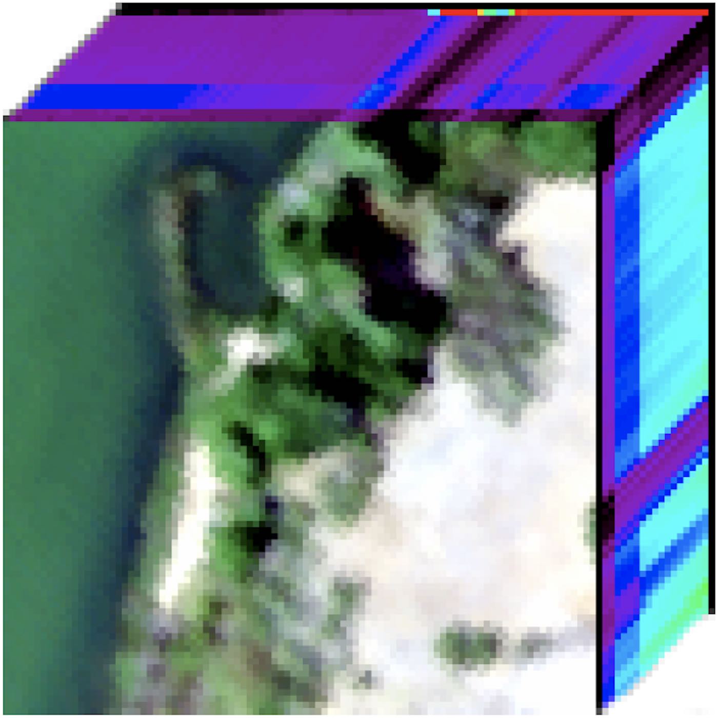
(a) Samson

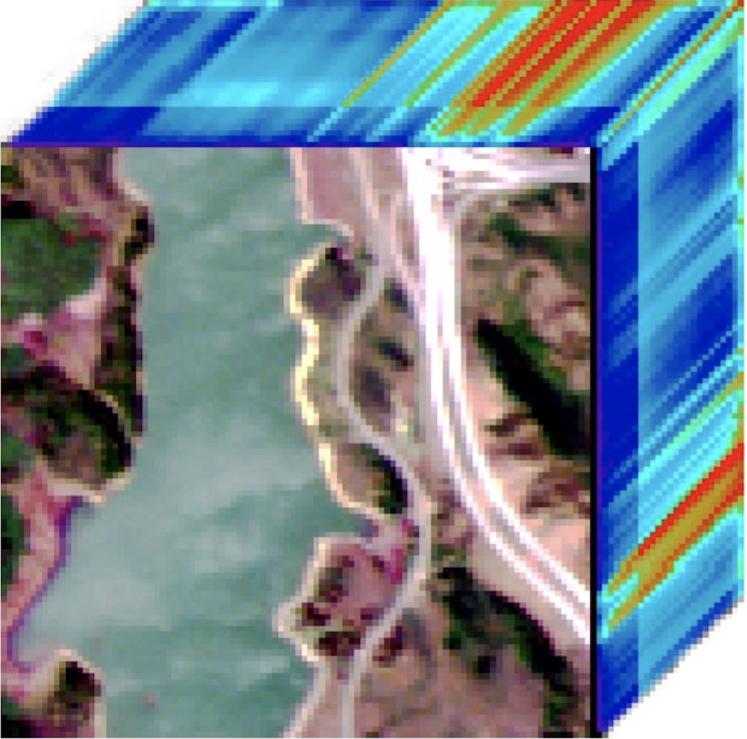
(b) Jasper Ridge

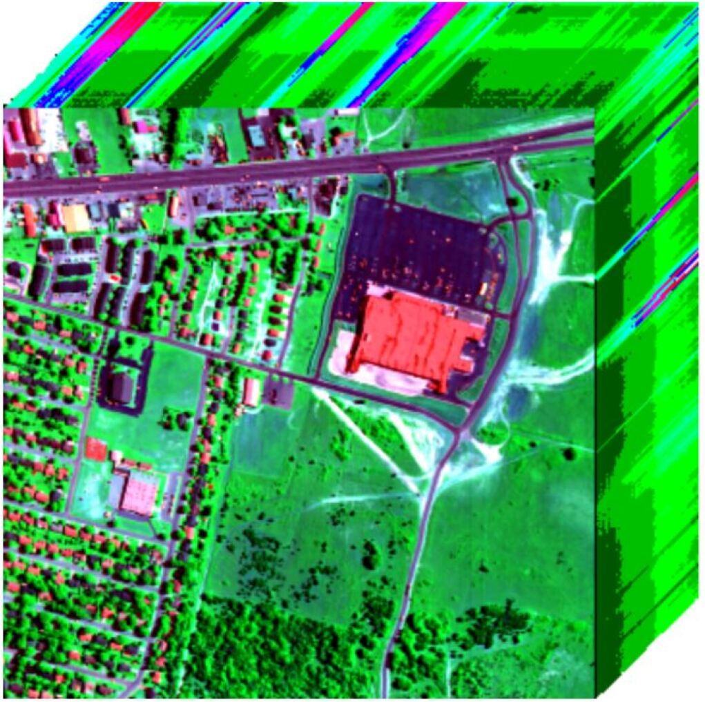
(c) Urban

Figure 1: Three real hyperspectral images

Since the groundtruth of abundance matrix $X$ does not satisfy the orthogonality constraints, the criteria utilized in the preceding subsection are not appropriate to measure the quality of hyperspectral unmixing. Here we consider spectral angle distance (SAD) (see for instance [61]) to evaluate the performance of algorithms. SAD uses an angle distance between groundtruth and estimated endmembers to measure the accuracy of endmember estimation. It is defined as $\text{SAD}\coloneqq\frac{1}{k}\sum_{i=1}^{k}\arccos\left(\frac{y_{i}^{\top}\hat{y_{i}}}{\|y_{i}\|\|\hat{y_{i}}\|}\right),$ where $\hat{y_{i}}$ and $y_{i}$ are estimation of $i$-th endmember and its corresponding groundtruth. Smaller SAD corresponds to better performance. Since other algorithms cannot generate a solution of problem (1.3) with small feasibility violation, in order to keep a fair comparison, we perform the rounding procedure and postprocessing on the solution generated by each method. Note that the postprocessing problem (3.1) is easy to solve, it mainly needs to find the maximum singular value and corresponding singular vector for $k$ small scale matrices.

The unmixing results of Samson, Jasper Ridge and Urban are illustrated in Fig. 2, Fig. 3 and Fig. 4, respectively. For Samson image, our method and ONP-MF are able to separate three endmembers, while the rest methods mix them together. For Jasper Ridge image, none of the methods can identify the road endmember, while our method and K-means can split water from other endmembers completely. All of algorithms perform relatively well on Urban dataset except for K-means, being able to separate four endmembers.

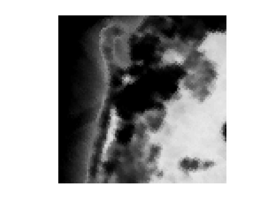
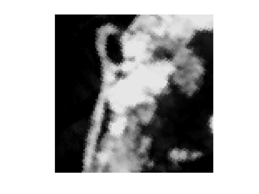
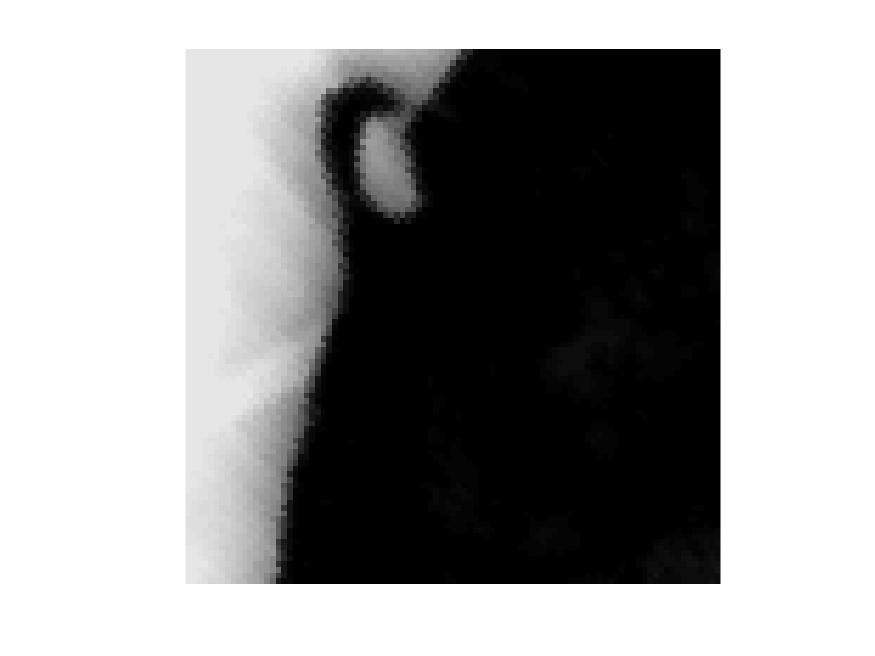
(a) ​​ground truth

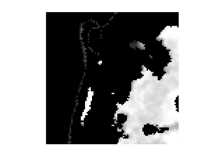
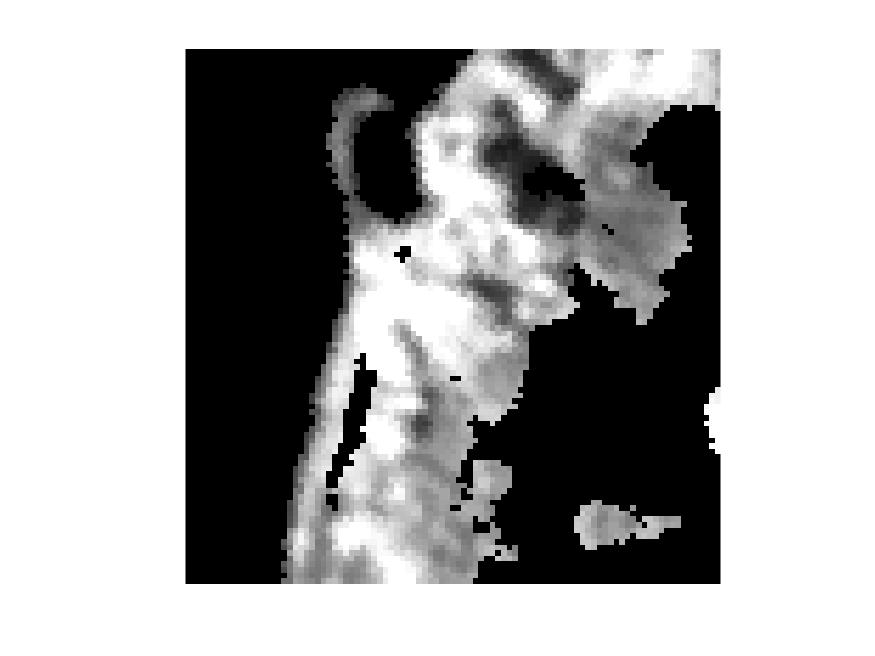
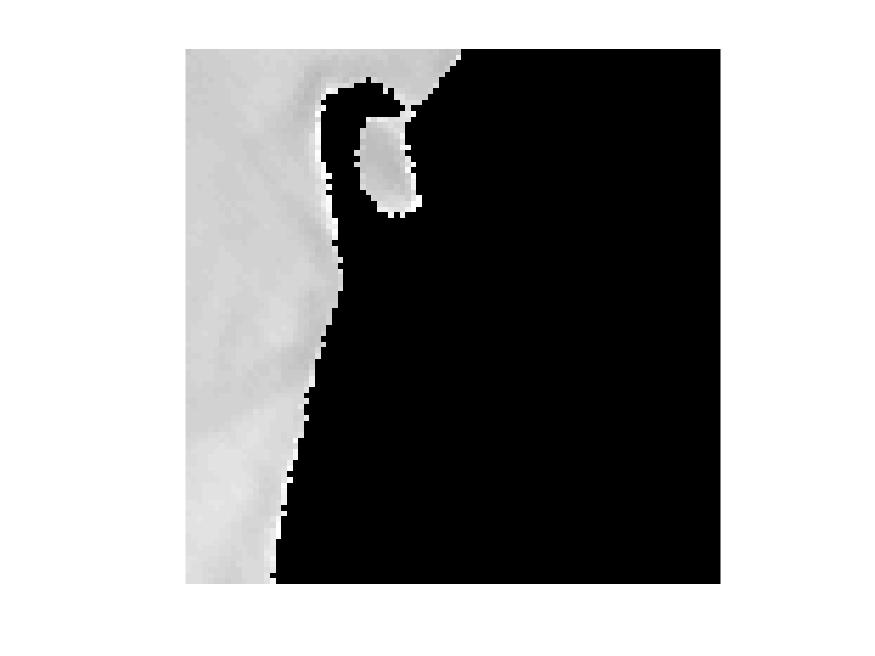
(b) ​EP4Orth+

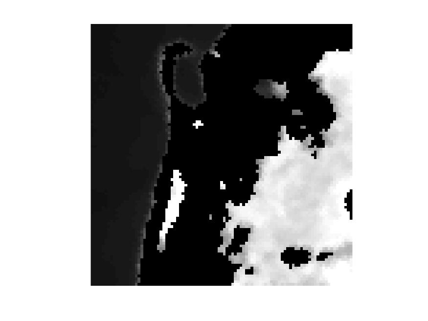
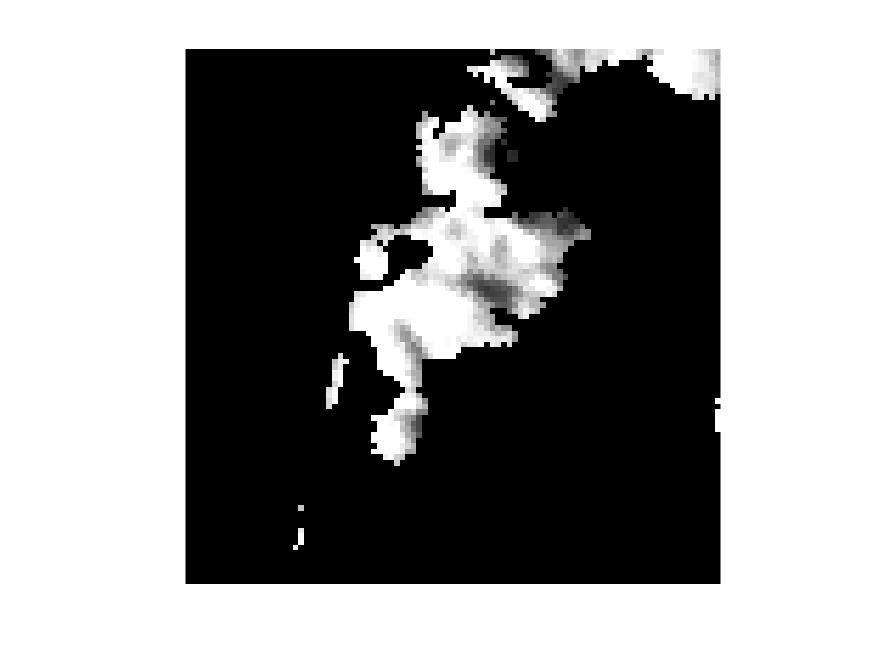
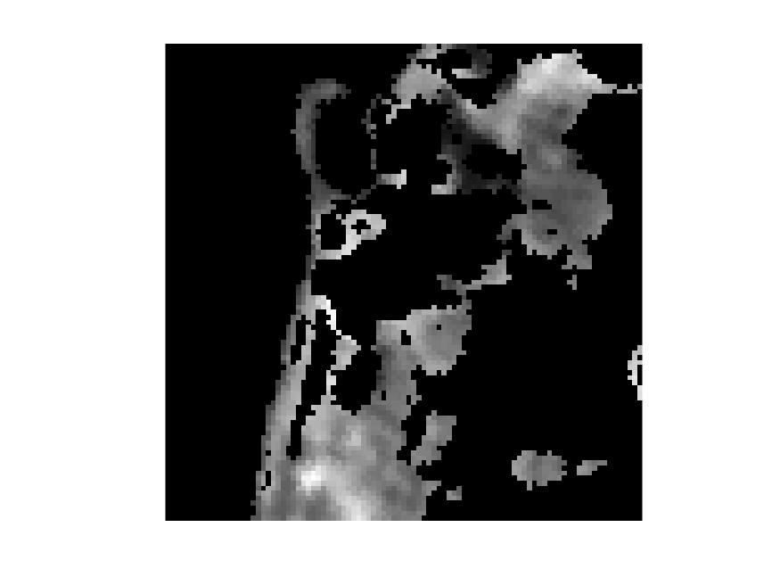
(c) U-onmf

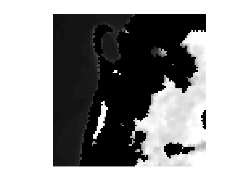
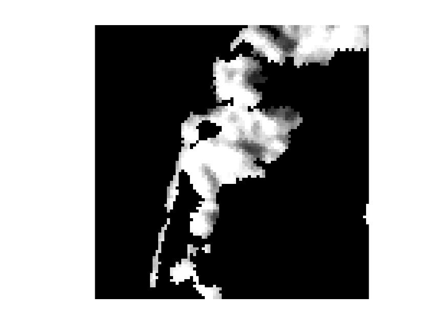
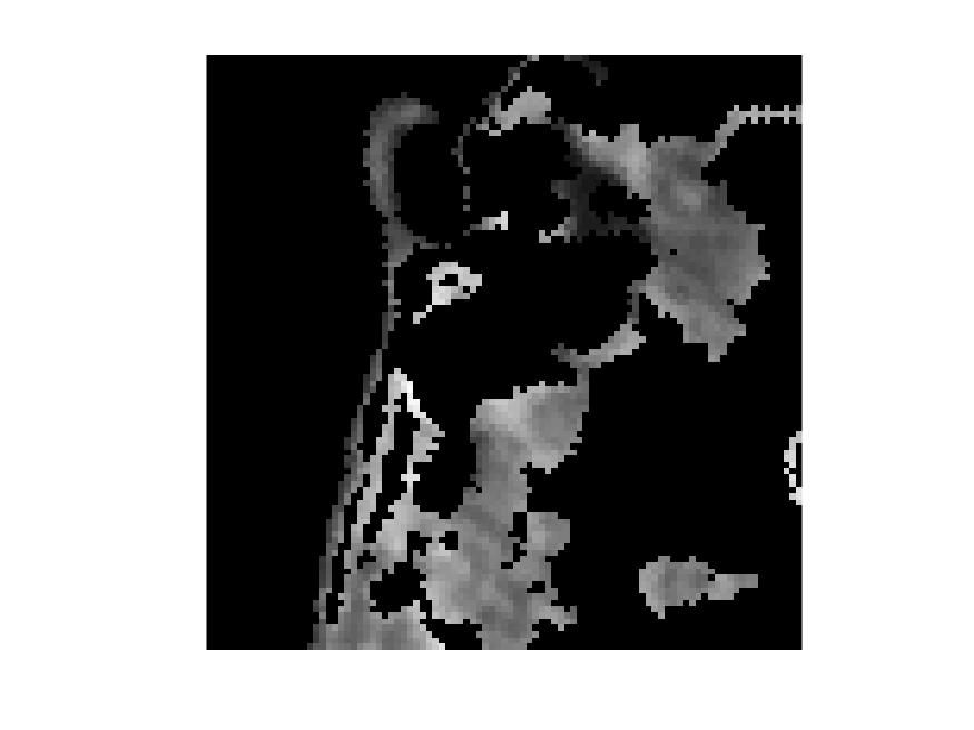
(d) OPNMF

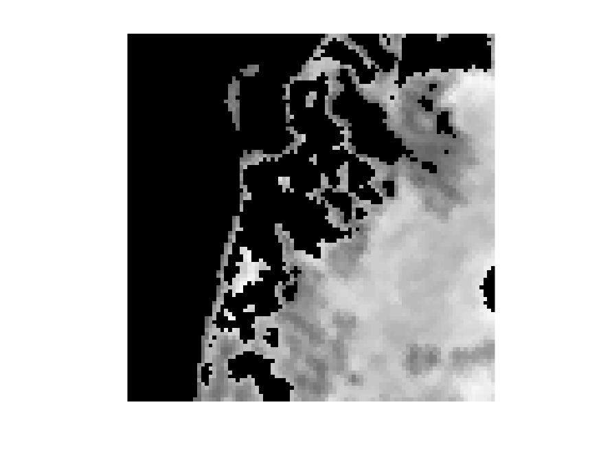
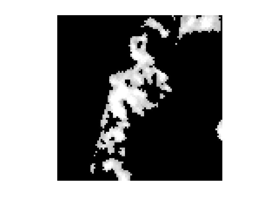
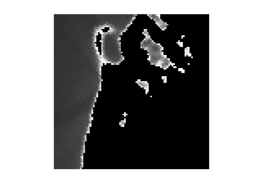
(e) K-means

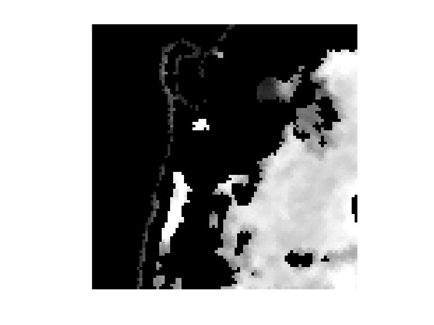
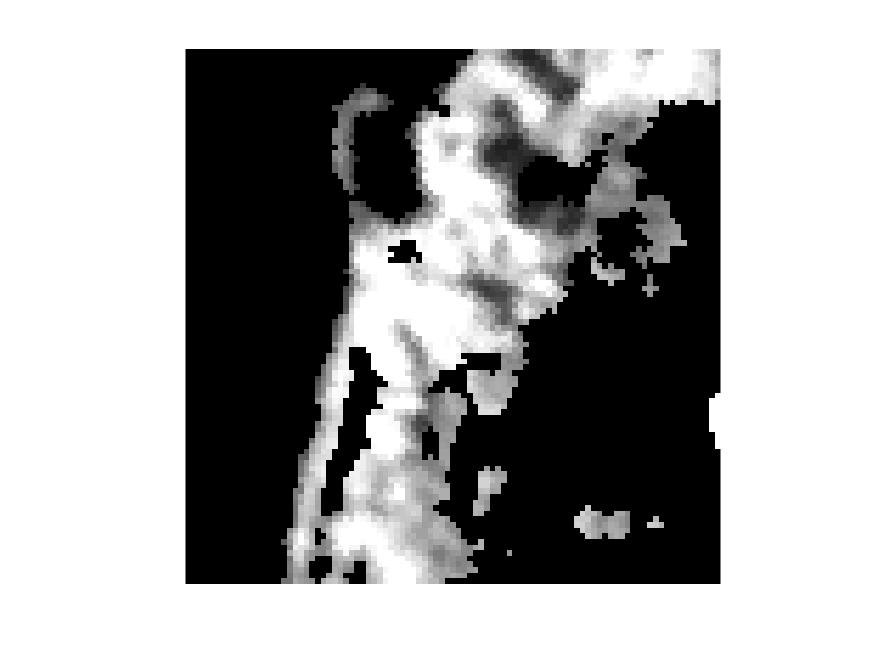
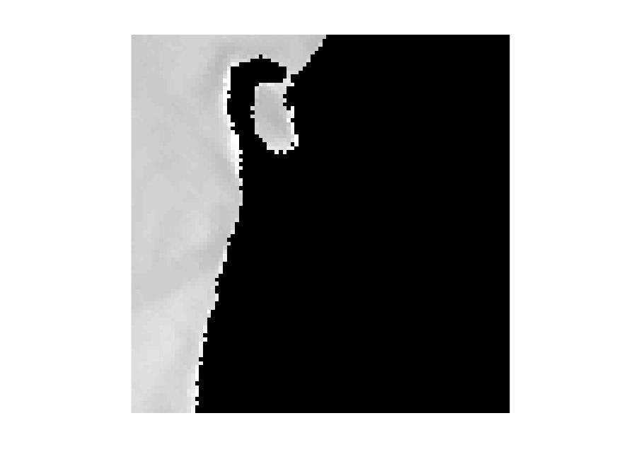
(f) ONP-MF

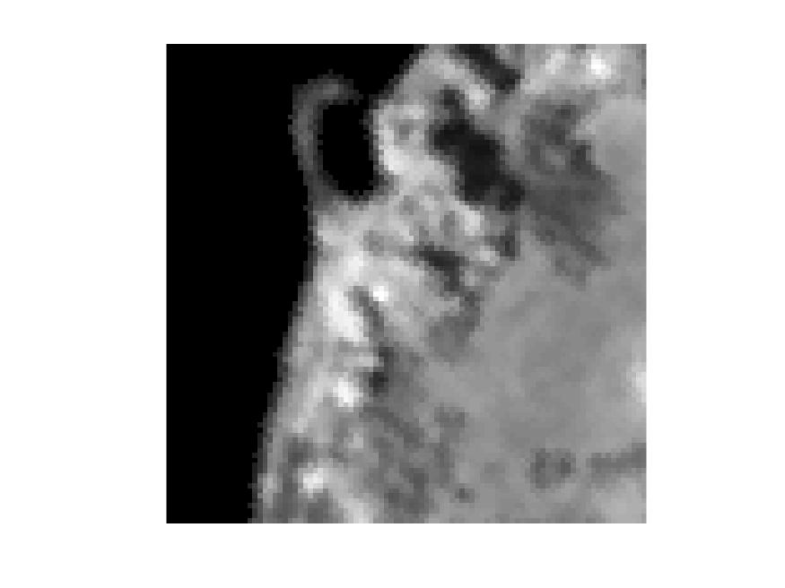
(g) EM-onmf

Figure 2: Unmixing results of Samson, from top to bottom: rock, tree, water.

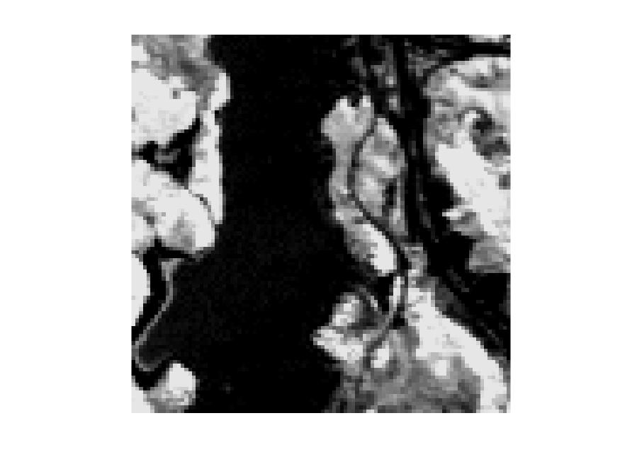
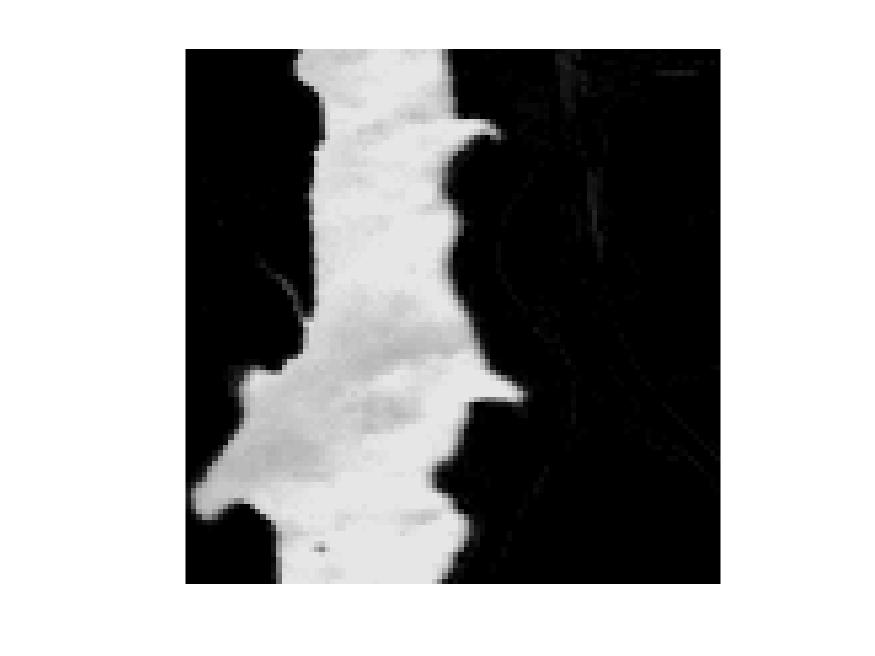
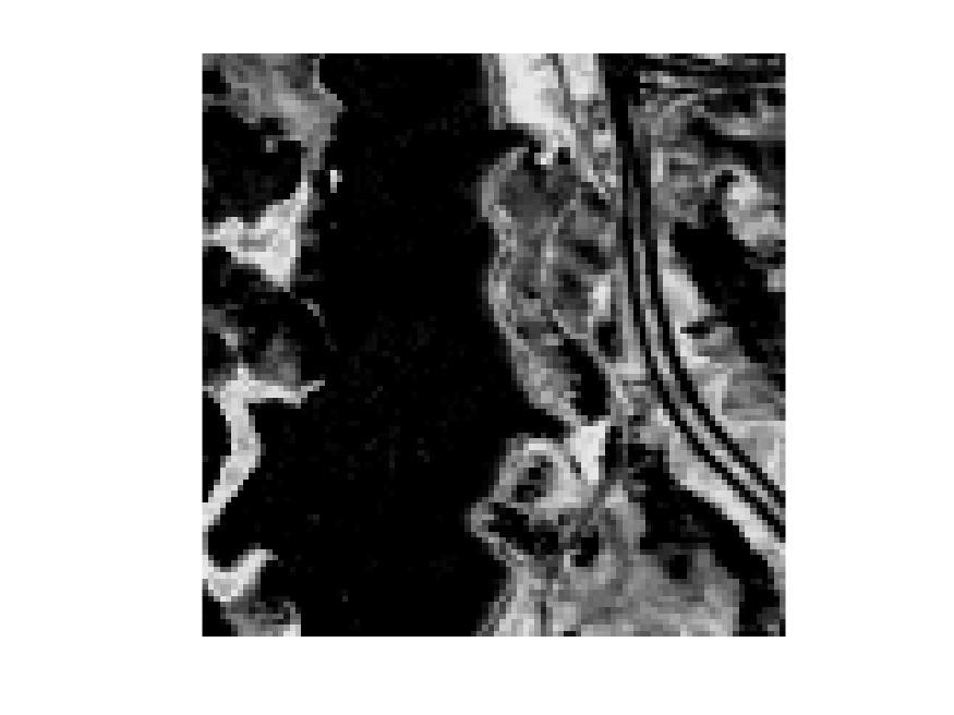
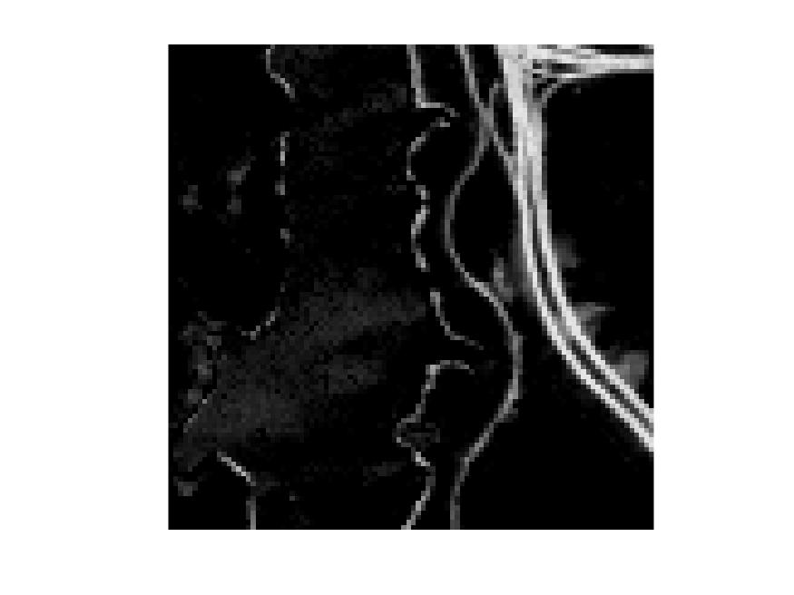
(a) ​​ground truth

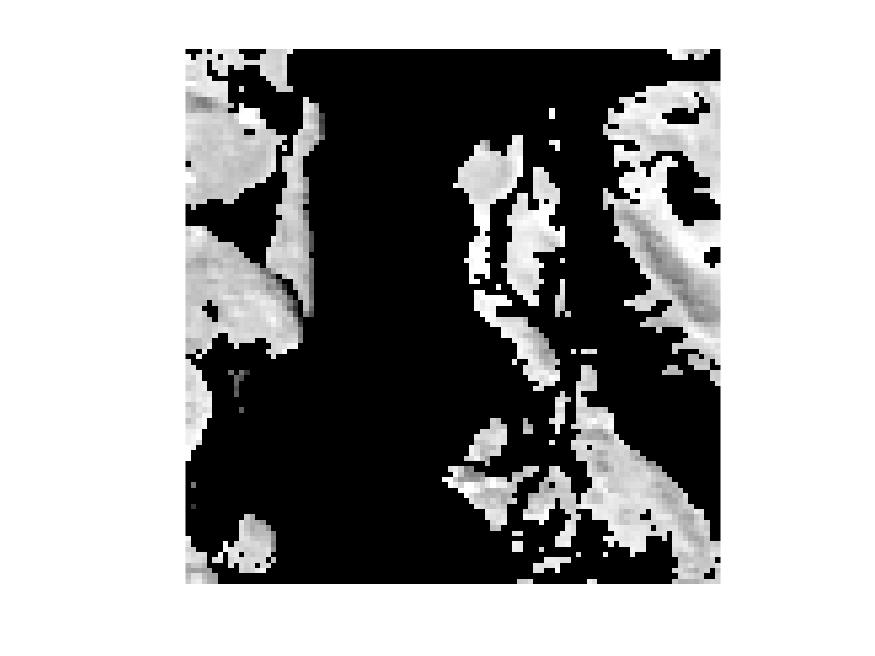
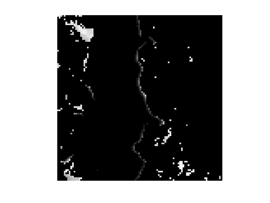
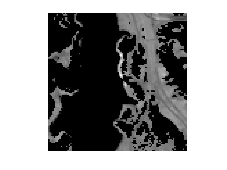
(b) ​EP4Orth+

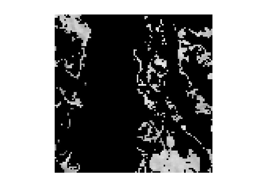
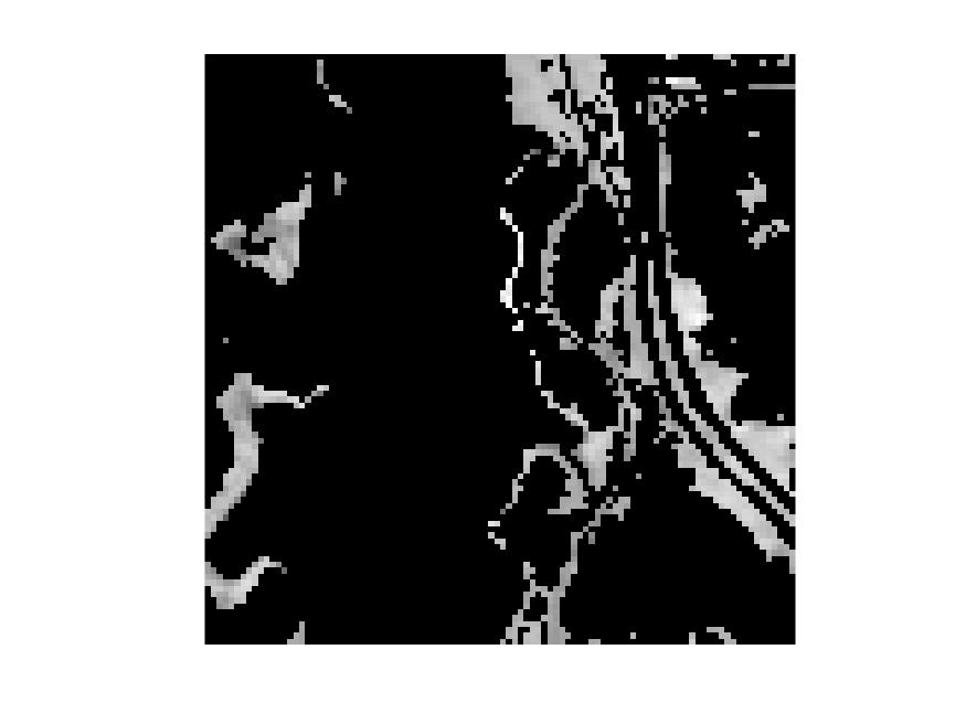
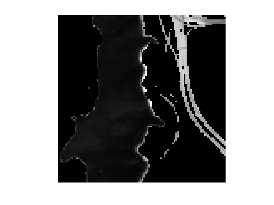
(c) U-onmf

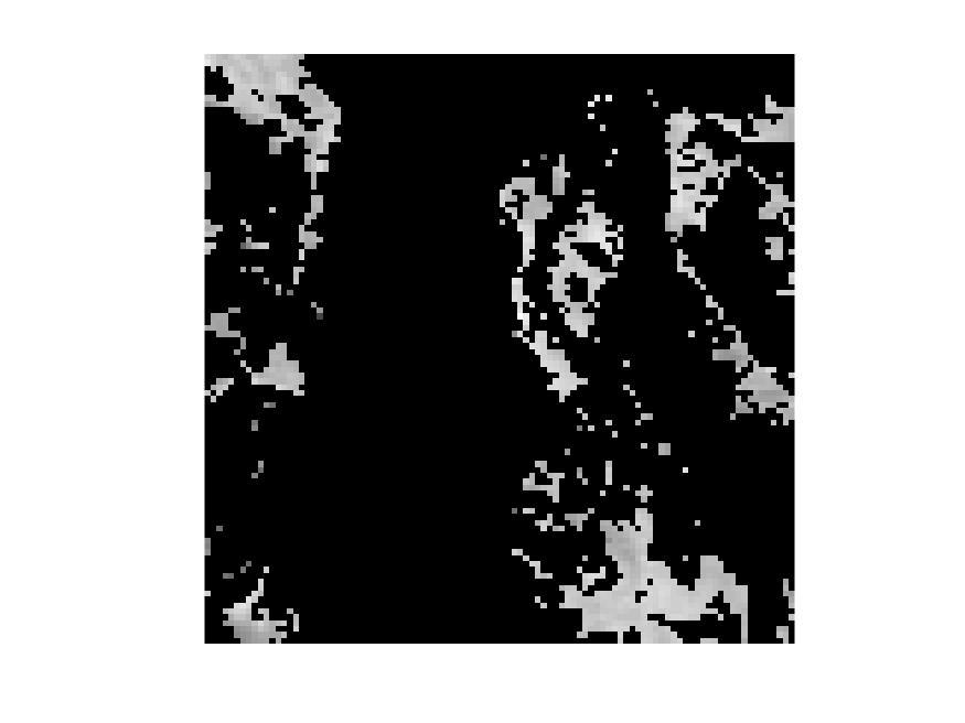
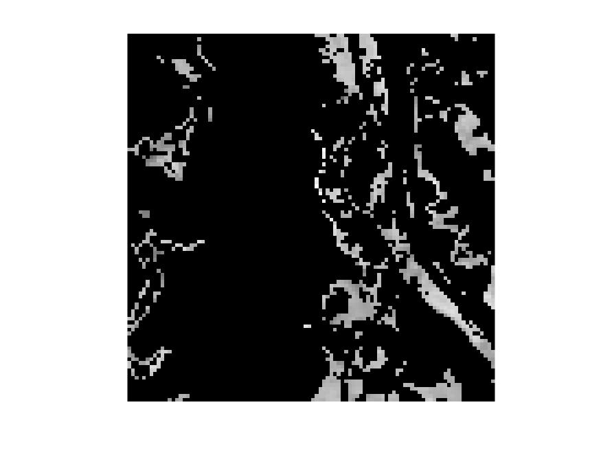
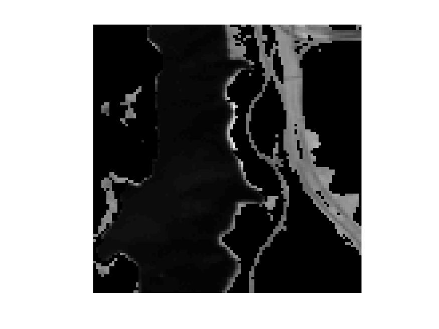
(d) OPNMF

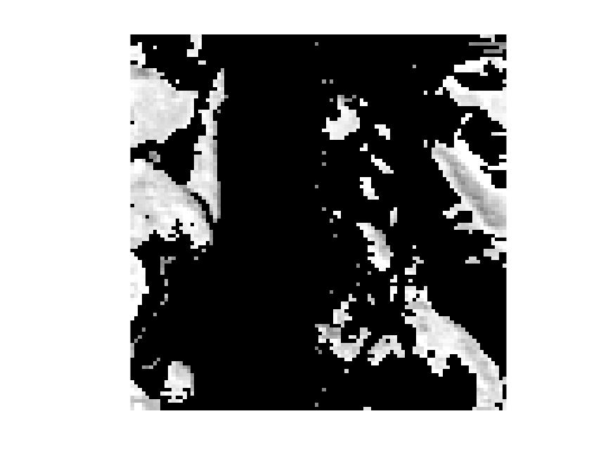
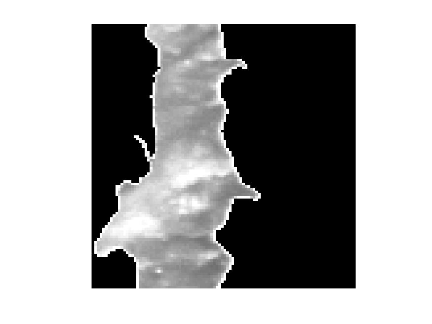
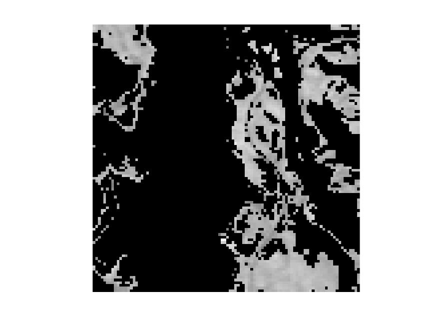
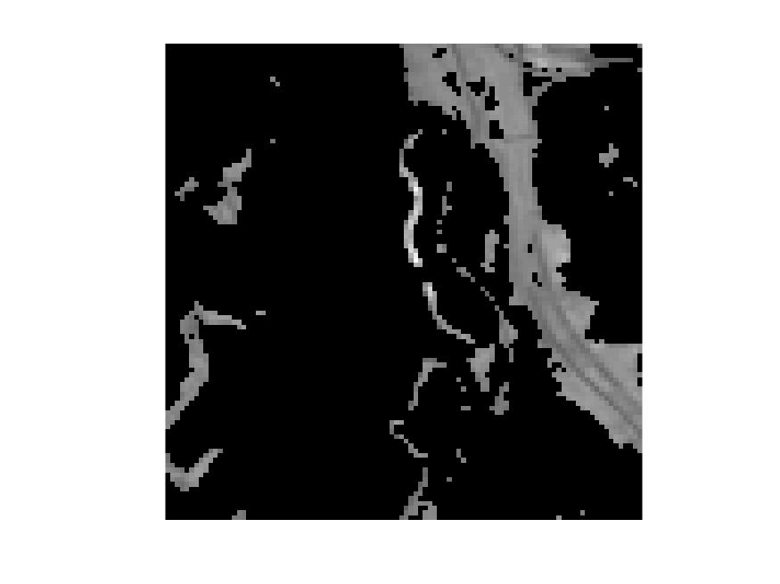
(e) K-means

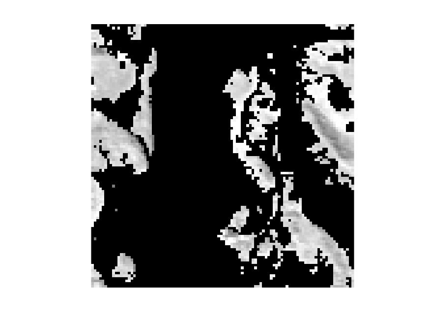
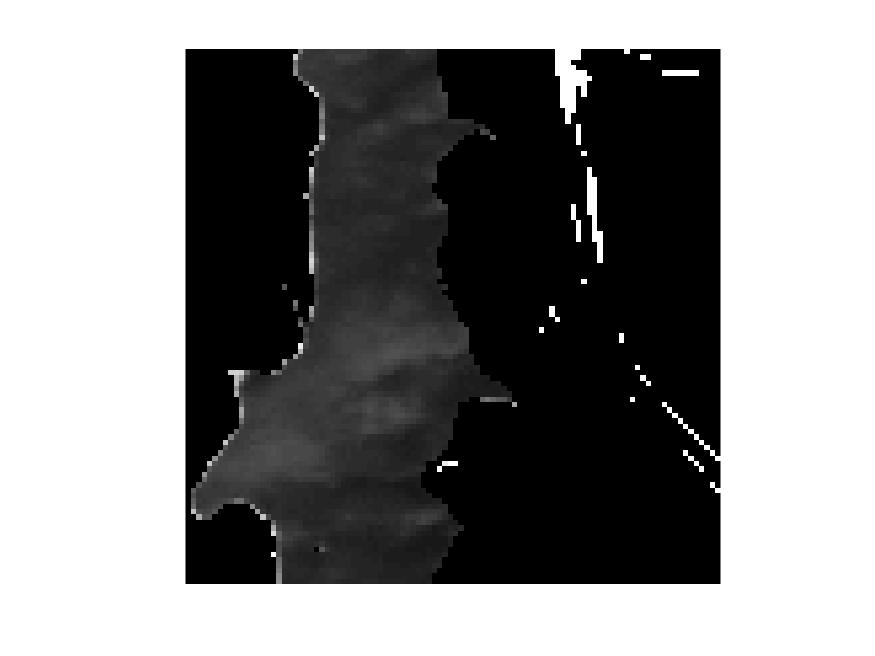
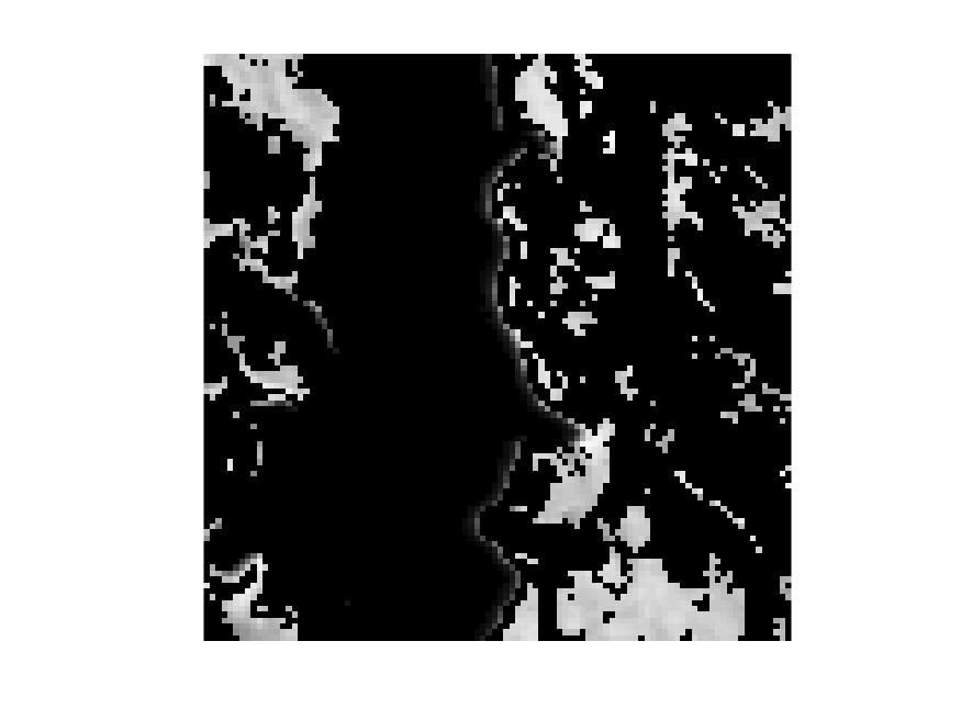
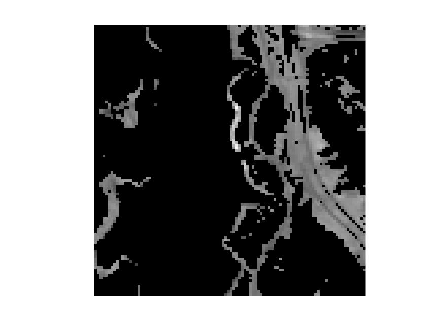
(f) ONP-MF

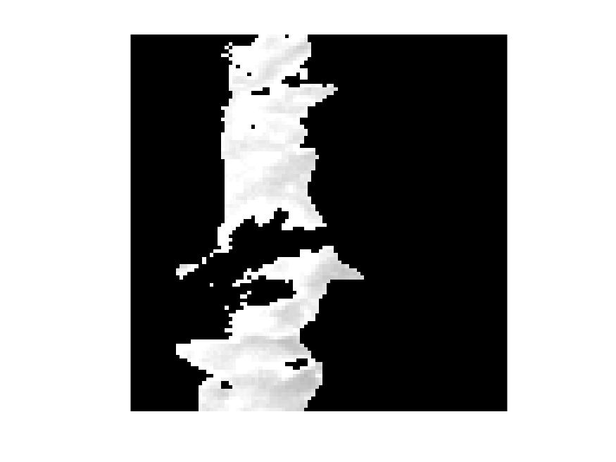
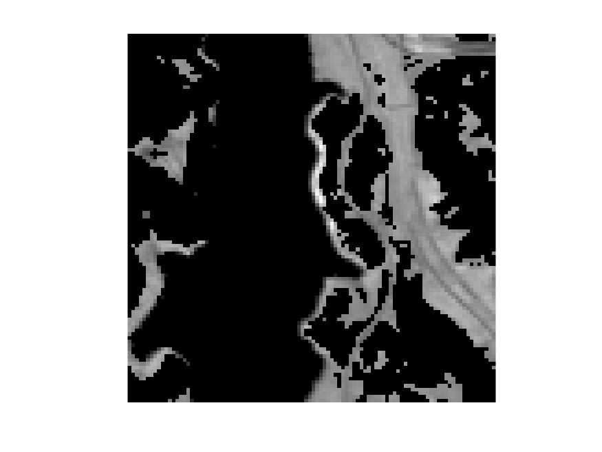
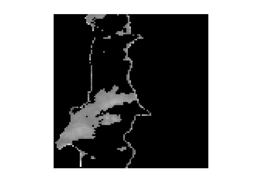
(g) EM-onmf

Figure 3: Unmixing results of Jasper Ridge, from top to bottom: tree, water, dirt, road

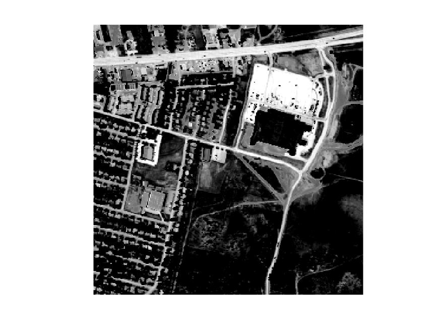
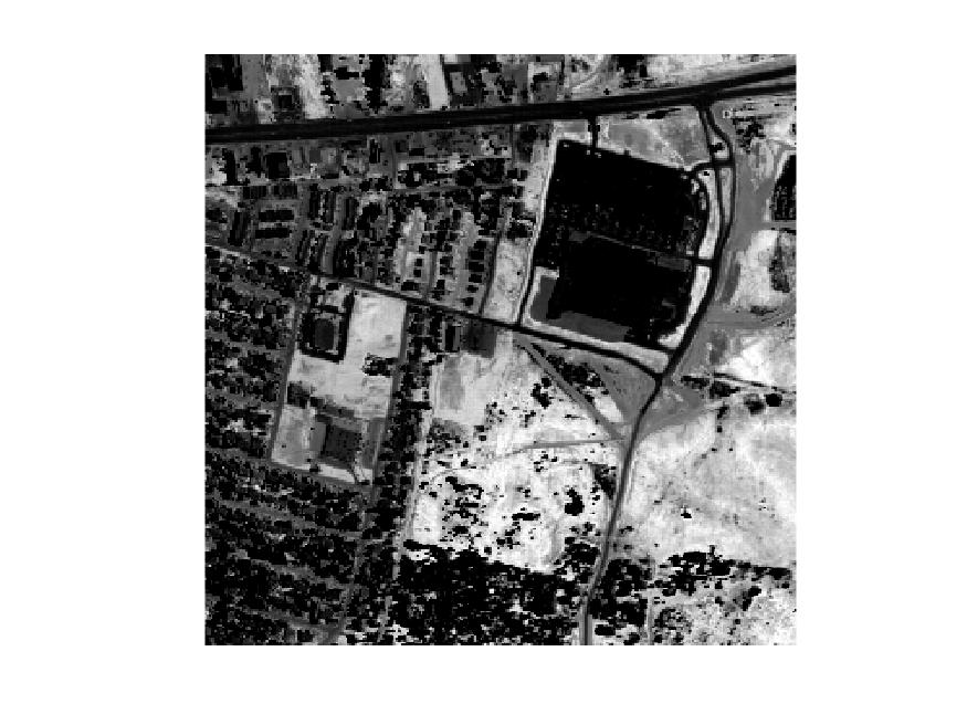
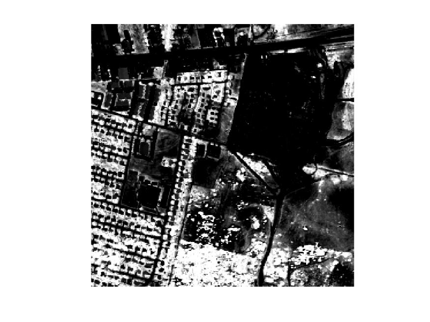
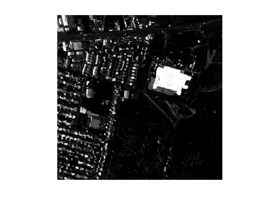
(a) ​​ground truth

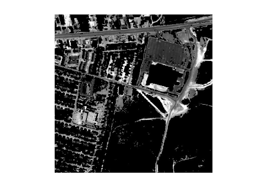
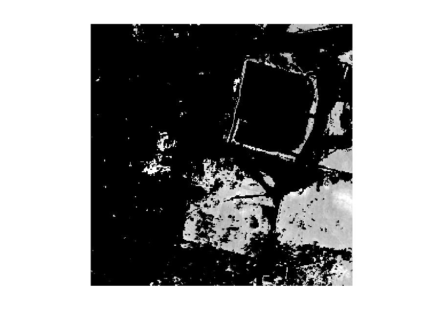
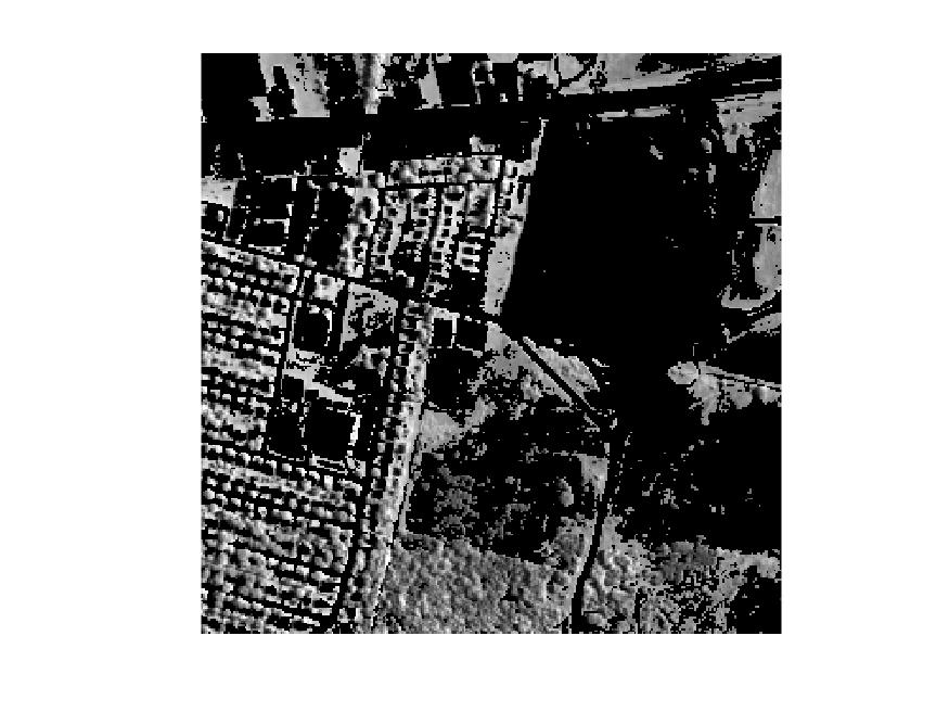
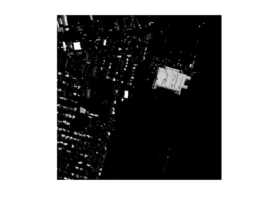
(b) ​our method

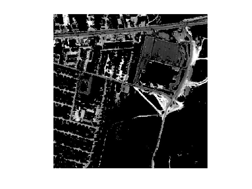
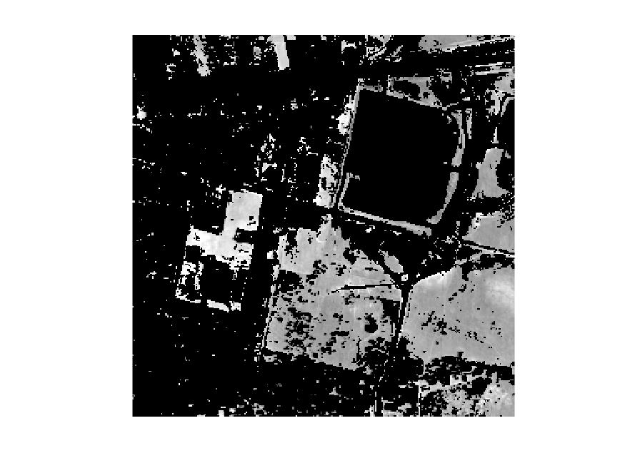
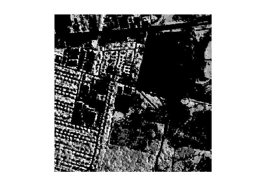
(c) U-onmf

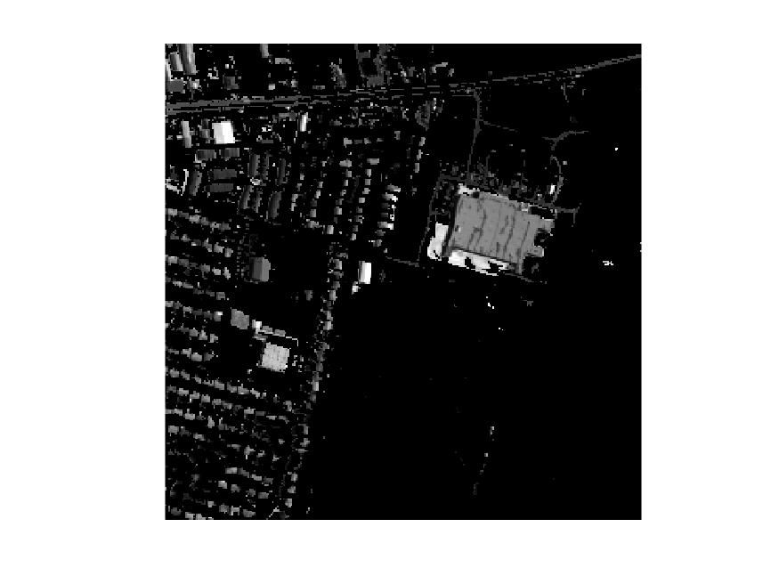
(d) OPNMF

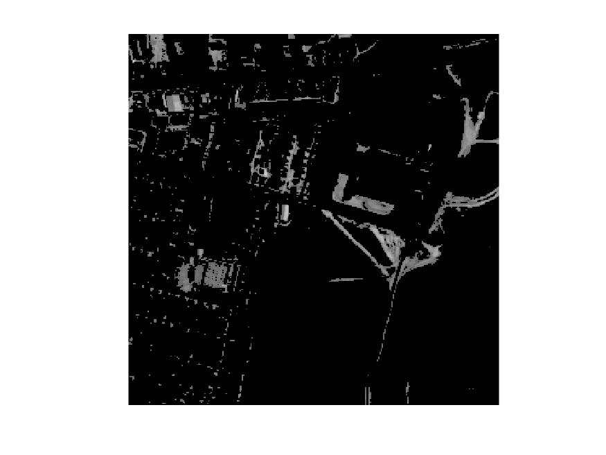
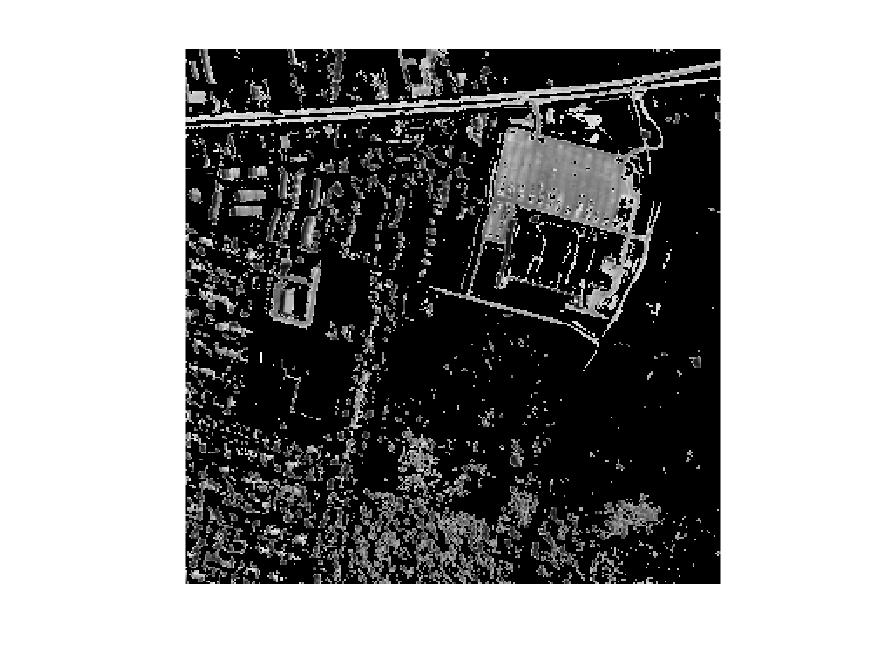
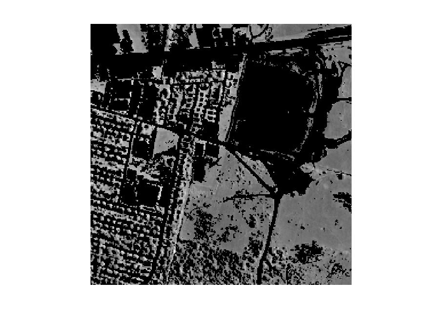
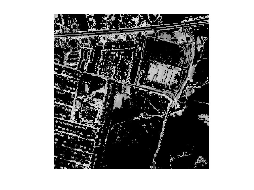
(e) K-means

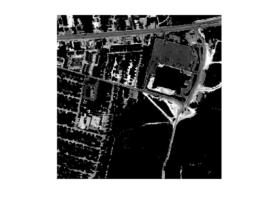
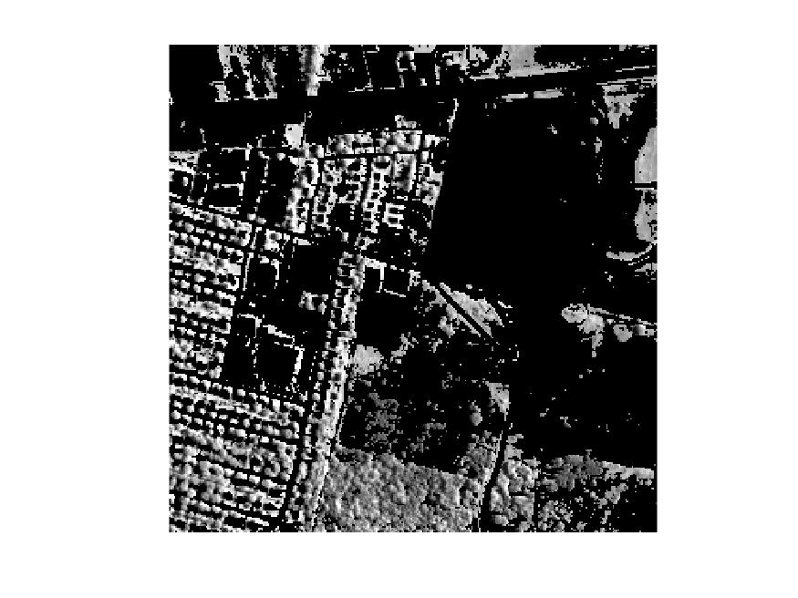
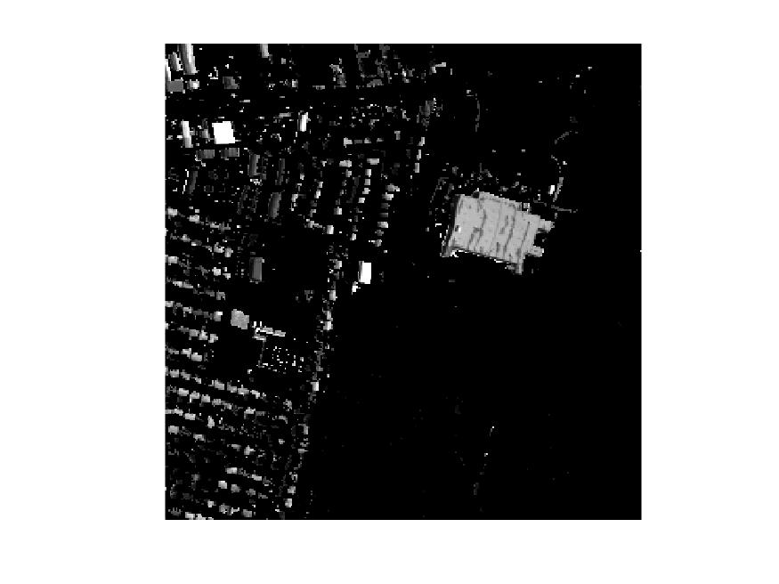
(f) ONP-MF

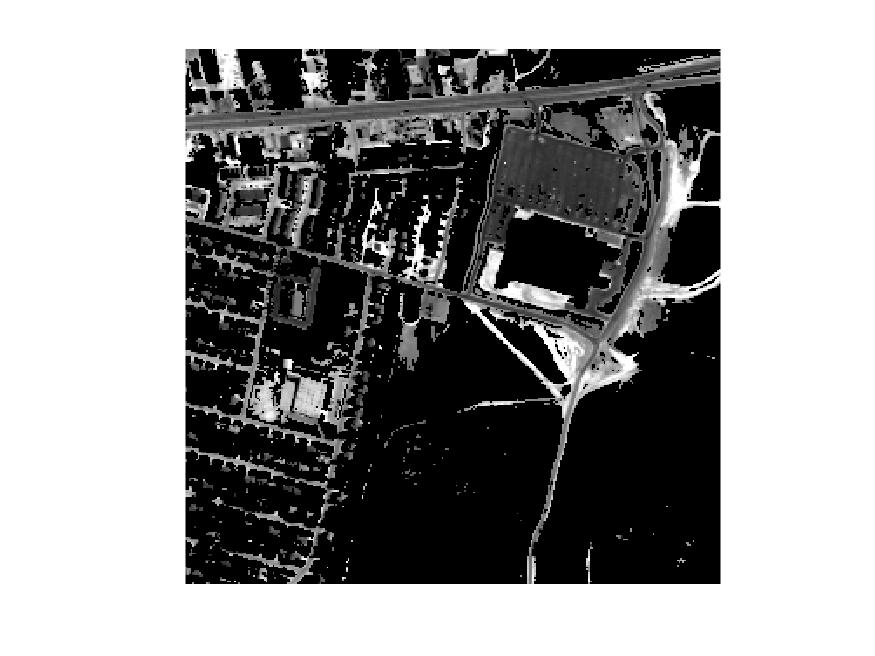
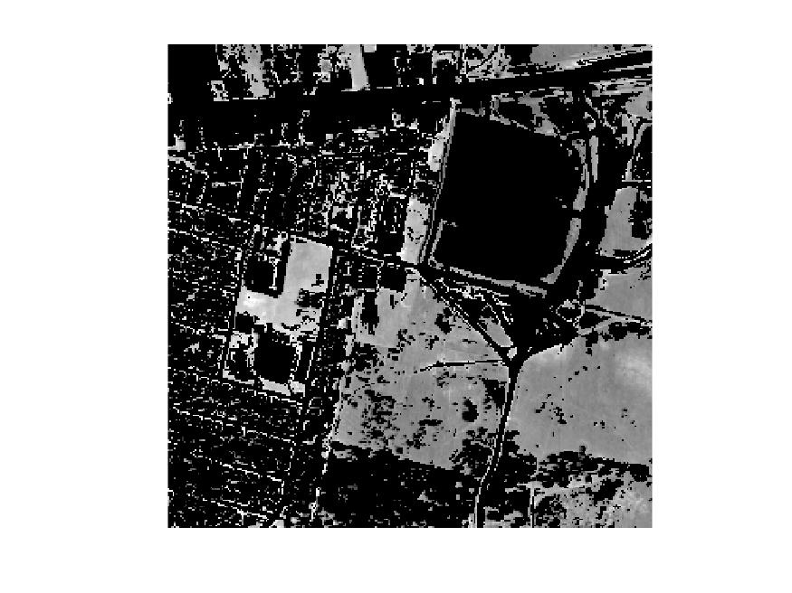
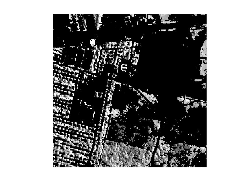
(g) EM-onmf

Figure 4: Unmixing results of Urban, from top to bottom: asphal, grass, tree, roof

Finally, we report in Table 5 the SAD and time cost for the three hyperspectral image datasets. From this table, we know that the efficiency of the proposed method is competitive to other algorithms. Particularly, our method achieves satisfying SAD among all algorithms. Besides, although EM-onmf is faster than our method on these datasets, the unmixing quality given by EM-onmf is unstable.

Table 5: Results on the hyperspectral image datasets.

	Samson		Jasper Ridge		Urban
method	SAD	time(s)	SAD	time(s)	SAD	time(s)
EP4Orth+	0.081	1.0	0.150	1.3	0.114	22
U-onmf	0.365	10	0.306	19	0.128	99
OPNMF	0.348	44	0.336	85	0.132	545
K-means	0.296	0.2	0.174	0.4	0.266	4
ONP-MF	0.085	16	0.276	34	0.112	339
EM-onmf	0.196	0.4	0.192	0.8	0.091	17

6.3 K-indicators model

We first remove the zero norm constraints from (1.5). The exact penalty model (4.25) with $p=1$, $q=2$, and $\epsilon=0$ for solving the K-indicator model becomes

(6.3) $$\min_{X\in\mathcal{OB}^{n,k}_{+},Y\in\mathcal{S}^{k,k}}\,\left\{\widehat{P}_{\sigma}(X,Y):=\|UY-X\|_{\mathtt{F}}^{2}+\sigma\|XV\|_{\mathtt{F}}^{2}\right\},$$

which is further equivalent to

(6.4) $$\min_{X\in\mathcal{OB}^{n,k}_{+},Y\in\mathcal{S}^{k,k}}\,\left\{P_{\sigma}(X,Y):=-\frac{1}{\sigma}\langle UY,X\rangle+\frac{1}{2}\|XV\|_{\mathtt{F}}^{2}\right\}.$$

With a fixed $Y$, (6.4) is exactly (6.2) with $C=UY$. Similar to the discussion therein, we obtain the main PALM iterations [12] for solving (6.4) in Algorithm 2 as

(6.5a) $$Y^{l+1}=\Pi_{\mathcal{S}^{k,k}}\left(\beta^{-1}Y^{l}+U^{\top}X^{l}\right),\quad\beta>0,$$

(6.5b) $$X^{l+1}\ \in\ \Pi_{\mathcal{OB}^{n,k}_{+}}\left(X^{l}-\alpha\left(X^{l}VV^{\top}-UY^{l+1}/\sigma\right)\right),\quad 0<\alpha<1.$$

Theorem 1 in [12] tells that the sequence $\{(X^{l},Y^{l})\}$ generated by (6.5a) and (6.5b) converges to a stationary point of (6.4). However, we find the convergence is slow if we fix the constant stepsizes $\alpha$ and $\beta$. Note that the closed form solution of (6.4) with respect to $Y$ for a fixed $X=X^{l}$ is $\Pi_{\mathcal{S}^{k,k}}\left(U^{\top}X^{l}\right)$, which corresponds to setting $\beta=+\infty$ in (6.5a). For the tested problem, by some easy calculations, we can see $\alpha_{\mathtt{LBB}}^{l}\geq 1$. The practical PALM iterations for solving (6.4) is thus given as

(6.6a) $$Y^{l+1}=\Pi_{\mathcal{S}^{k,k}}\left(U^{\top}X^{l}\right).$$

(6.6b) $$X^{l+1}\ \in\ \Pi_{\mathcal{OB}^{n,k}_{+}}\left(X^{l}-\alpha^{l}\left(X^{l}VV^{\top}-UY^{l+1}/\sigma\right)\right),\ \alpha^{l}=\min\{\alpha_{\mathtt{LBB}}^{l},10k\}.$$

The flops for (6.6a) and (6.6b) are $2nk^{2}+O(k^{3})$ and $2nk^{2}+O(nk)$, respectively.

Chen et al. [19] proposed a semi-convex relaxation model to solve (1.5). Their intermediate model corresponds to (6.3) with $\sigma=0$ and $\mathcal{OB}^{n,k}_{+}$ replaced by $\{X\in\mathbb{R}^{n\times k}:0\leq X\leq 1\}$. A double-layered alternating projection framework was investigated in [19] to solve the relaxation model. The method was named KindAP. To evaluate the efficiency of our method, we compare it with KindAP (downloaded from https://github.com/yangyuchen0340/Kind) on data clustering problems. We adopt eight image datasets, including catsndogs, ORL, CIFAR (train and test), COIL100, flower, omniglot, and UKBench. We set $\gamma_{2}=10$, $\sigma_{0}=10$, $\eta=0.5$ and $\mathrm{tol}^{\mathrm{feas}}=0.1$ and $X^{0}=\Pi_{\mathcal{OB}^{n,k}_{+}}(U)$ in our method. The initial points of KindAP is set as $\Pi_{\mathbb{R}^{n,k}_{+}}(U)$. Similar as in section 6.2.2, purity, entropy and NMI are adopted to judge the performance of proposed algorithms. The results are presented in Table 6. It shows that the clustering results given by our methods are comparable to that provided by KindAP, which means both methods are able to solve (1.5) with a relatively high quality. On the other hand, our algorithm is generally faster than KindAP. Our algorithm is especially efficient on datasets omniglot and UKbench, in which the number of clusters is relatively large. Besides, it should be mentioned that although we relax the zero norm constraints from problem (1.5), the matrix $X$ we obtained is always feasible to (1.5). By contrast, the matrix $X$ returned by KindAP may not be an orthogonal nonnegative matrice although it always satisfies the zero norm constraints.

Table 6: Comparison of KindAP and our methods on data clustering problems. In the table, “a” and “b” stand for KindAP and EP4Orth+, respectively. Results marked in bold mean better performance in the corresponding index.

			purity(%)		NMI(%)		entropy(%)		time(s)
datasets	$n$	$k$	a	b	a	b	a	b	a	b
catsndogs	4000	2	96.20	96.23	76.80	76.96	23.20	23.04	0.03	0.02
ORL	400	40	87.75	88.00	92.94	92.76	7.06	7.24	0.04	0.01
CIFAR100-test	10000	100	69.42	69.44	71.34	71.36	28.66	28.64	0.63	0.41
CIFAR100-train	50000	100	99.63	99.63	99.57	99.57	0.43	0.43	3.13	1.66
COIL100	7200	100	91.93	91.93	97.30	97.41	2.70	2.59	1.47	0.44
flower	2040	102	44.95	44.90	63.52	63.40	36.48	36.60	0.58	0.42
omniglot	17853	1623	21.95	21.97	70.86	70.94	29.14	29.06	1176	432
UKBench	10200	2550	90.64	91.04	97.64	97.76	2.36	2.24	3215	1268

7 Concluding remarks

In this paper, we consider optimization with nonnegative and orthogonality constraints. We focus on an equivalent formulation of the concerned problem, and show that the two formulations share the same minimizers and first- and second-order optimality conditions. By estimating a local error bound of $\mathcal{S}^{n,k}_{+}$, we provide a general class of exact and possibly smooth penalty models as well as a practical penalty algorithm with postprocessing. We investigate the asymptotic convergence of the penalty method and show that any limit point is a weakly stationary point of the concerned problem and becomes a stationary point under some more mild conditions. A second-order method for solving the penalty subproblem, namely, optimization with nonnegative and multiple spherical constraints, is also given. Our numerical results show that the proposed penalty method performs well for the projection problem, ONMF and the K-indicators model and it can always return high quality orthogonal nonnegative matrices.

Appendix A Construction of problem (6.1) with unique solution

Proposition.

Choose $X^{*}\in\mathcal{S}^{n,k}_{+}$ and $L\in\mathbb{R}^{k\times k}$ with positive diagonal elements satisfying $L_{ii}L_{jj}>\max\{L_{ij},L_{ji},0\}^{2}\ \forall i,j\in[k],i\neq j.$ Then the optimal solution of (6.1) with $C=X^{*}L^{\top}$ is unique and exactly $X^{*}$.

Proof.

For simplicity of notation, we use $\sum_{i}$ to denote $\sum_{i\in[k]}$ in the proof. Since problem (6.1) is equivalent to $\max_{X\in\mathcal{S}^{n,k}_{+}}\,\langle C,X\rangle$, we only need to show that $\langle C,Y\rangle<\langle C,X^{*}\rangle=\sum_{i}L_{ii}$, $\forall\ \mathcal{S}^{n,k}_{+}\owns Y\neq X^{*}$. Let $Z=\mathsf{sgn}(Y)$ and $P=\Pi_{\mathbb{R}_{+}^{n}}(L)$. We have

(A.1) $$\langle C,Y\rangle=\mathrm{tr}(L(X^{*})^{\top}Y)=\sum\nolimits_{i}\sum\nolimits_{j}L_{ji}\mathbf{y}_{i}^{\top}\mathbf{x}^{*}_{j}\leq\sum\nolimits_{i}\sum\nolimits_{j}P_{ji}\mathbf{y}_{i}^{T}(\mathbf{x}^{*}_{j}\circ\mathbf{z}_{i}).$$

Define $w_{ji}=\|\mathbf{x}_{j}^{*}\circ\mathbf{z}_{i}\|^{2}$. With $X^{*}\in\mathcal{S}^{n,k}_{+}$, we have $\|\sum_{j}P_{ji}(\mathbf{x}_{j}^{*}\circ\mathbf{z}_{i})\|$ = $(\sum_{i}P_{ji}^{2}w_{ji})^{1/2}$. Using the Cauchy-Schwarz inequality, $\|\mathbf{y}_{i}\|=1$ and the requirements on $L$, we have

(A.2) $$\sum\nolimits_{j}P_{ji}\mathbf{y}_{i}^{T}(\mathbf{x}^{*}_{j}\circ\mathbf{z}_{i})\leq\Big{(}\sum\nolimits_{j}P^{2}_{ji}w_{ji}\Big{)}^{\frac{1}{2}}\leq P_{ii}\Big{(}\sum\nolimits_{j}\frac{P_{jj}}{P_{ii}}w_{ji}\Big{)}^{\frac{1}{2}}.$$

With (A.1) and $\langle C,X^{*}\rangle=\sum_{i}L_{ii}=\sum_{i}P_{ii}$, we further have

(A.3) $$\langle C,Y\rangle\leq\sum\nolimits_{i}P_{ii}\Big{(}\sum\nolimits_{j}\frac{P_{jj}}{P_{ii}}w_{ji}\Big{)}^{\frac{1}{2}}\leq\Big{(}\sum\nolimits_{i}P_{ii}\Big{)}^{\frac{1}{2}}\Big{(}\sum\nolimits_{i}\sum\nolimits_{j}P_{jj}w_{ji}\Big{)}^{\frac{1}{2}}\leq\langle C,X^{*}\rangle,$$

where the second inequality uses the fact that $\sum_{i}a_{i}x_{i}^{\frac{1}{2}}\leq(\sum_{i}a_{i})^{\frac{1}{2}}(\sum_{i}a_{i}x_{i})^{\frac{1}{2}}$ for $a_{i}>0$ and $x_{i}\geq 0$, and the third inequality uses $\sum_{i}w_{ji}\leq 1$. Obviously, the equalities in (A.2) and (A.3) hold if and only if $Y=X^{*}$. The proof is completed.

References

• [1] P.-A. Absil, R. Mahony, and R. Sepulchre, Optimization algorithms on matrix manifolds, Princeton University Press, 2009.
• [2] R. Andreani, J. M. MartÍnez, A. Ramos, and P. J. Silva, A cone-continuity constraint qualification and algorithmic consequences, SIAM J. Optim., 26 (2016), pp. 96–110.
• [3] H. Attouch, J. Bolte, P. Redont, and A. Soubeyran, Proximal alternating minimization and projection methods for nonconvex problems: an approach based on the Kurdyka-Łojasiewicz inequality, Math. Oper. Res., 35 (2010), pp. 438–457.
• [4] H. Attouch, J. Bolte, and B. F. Svaiter, Convergence of descent methods for semi-algebraic and tame problems: proximal algorithms, forward–backward splitting, and regularized gauss–seidel methods, Math. Program., 137 (2013), pp. 91–129.
• [5] J. Barzilai and J. M. Borwein, Two-point step size gradient methods, IMA J. Numer. Anal., 8 (1988), pp. 141–148.
• [6] H. Bauschke, M. Bui, and X. Wang, Projecting onto the intersection of a cone and a sphere, SIAM J. Optim., 28 (2018), pp. 2158–2188.
• [7] R. Bergmann and R. Herzog, Intrinsic formulation of KKT conditions and constraint qualifications on smooth manifolds, SIAM J. Optim., 29 (2019), pp. 2423–2444.
• [8] L. Berk and D. Bertsimas, Certifiably optimal sparse principal component analysis, Math. Program. Comput., 11 (2019), pp. 381–420.
• [9] D. Bertsekas, Nonlinear programming, Athena Scientific, 1999.
• [10] D. P. Bertsekas, Constrained optimization and Lagrange multiplier methods, Academic press, 1996.
• [11] J. M. Bioucasdias, A. Plaza, N. Dobigeon, M. Parente, Q. Du, P. Gader, and J. Chanussot, Hyperspectral unmixing overview: Geometrical, statistical, and sparse regression-based approaches, IEEE J. Sel. Top. Appl. Earth Obs. Remote Sens., 5 (2012), pp. 354–379.
• [12] J. Bolte, S. Sabach, and M. Teboulle, Proximal alternating linearized minimization for nonconvex and nonsmooth problems, Math. Program., 146 (2014), pp. 459–494.
• [13] N. Boumal, P.-A. Absil, and C. Cartis, Global rates of convergence for nonconvex optimization on manifolds, IMA J. Numer. Anal., 39 (2019), pp. 1–33.
• [14] C. Boutsidis, P. Drineas, and M. W. Mahoney, Unsupervised feature selection for the $k$-means clustering problem, in NeurIPS, 2009, pp. 153–161.
• [15] C. Boutsidis and E. Gallopoulos, SVD based initialization: a head start for nonnegative matrix factorization, Pattern Recogn., 41 (2008), pp. 1350–1362.
• [16] D. Cai, Q. Mei, J. Han, and C. Zhai, Modeling hidden topics on document manifold, in Proceedings of the 17th ACM CIKM, ACM, 2008, pp. 911–920.
• [17] T. Carson, D. G. Mixon, and S. Villar, Manifold optimization for k-means clustering, in SampTA, IEEE, 2017, pp. 73–77.
• [18] K.-C. Chang, K. Pearson, and T. Zhang, Perron-Frobenius theorem for nonnegative tensors, Commun. Math. Sci., 6 (2008), pp. 507–520.
• [19] F. Chen, Y. Yang, L. Xu, T. Zhang, and Y. Zhang, Big-data clustering: K-means or k-indicators?, arXiv:1906.00938, (2019).
• [20] X. Chen, Z. Lu, and T. K. Pong, Penalty methods for a class of non-Lipschitz optimization problems, SIAM J. Optim., 26 (2016), pp. 1465–1492.
• [21] C. Ding, T. Li, W. Peng, and H. Park, Orthogonal nonnegative matrix t-factorizations for clustering, in Proceedings of the 12th ACM SIGKDD, ACM, 2006, pp. 126–135.
• [22] M. P. Friedlander and P. Tseng, Exact regularization of convex programs, SIAM J. Optim., 18 (2008), pp. 1326–1350.
• [23] B. Gao, X. Liu, and Y. Yuan, Parallelizable algorithms for optimization problems with orthogonality constraints, SIAM J. Sci. Comput., 41 (2019), pp. A1949–A1983.
• [24] J.-B. Hiriart-Urruty and A. Seeger, A variational approach to copositive matrices, SIAM Review, 52 (2010), pp. 593–629.
• [25] J. Hu, B. Jiang, L. Lin, Z. Wen, and Y. Yuan, Structured quasi-newton methods for optimization with orthogonality constraints, SIAM J. Sci. Comput., 41 (2019), pp. A2239–A2269.
• [26] J. Hu, A. Milzarek, Z. Wen, and Y. Yuan, Adaptive quadratically regularized Newton method for Riemannian optimization, SIAM J. Matrix Anal. Appl., 39 (2018), pp. 1181–1207.
• [27] B. Jiang, Y.-F. Liu, and Z. Wen, $l_{p}$-norm regularization algorithms for optimization over permutation matrices, SIAM J. Optim., 26 (2016), pp. 2284–2313.
• [28] N. Keshava and J. F. Mustard, Spectral unmixing, IEEE Signal Process. Mag., 19 (2002), pp. 44–57.
• [29] D. Kuang, C. Ding, and H. Park, Symmetric nonnegative matrix factorization for graph clustering, in Proceedings of the 2012 SDM, SIAM, 2012, pp. 106–117.
• [30] B. Li, G. Zhou, and A. Cichocki, Two efficient algorithms for approximately orthogonal nonnegative matrix factorization, IEEE Signal Process. Lett., 22 (2015), pp. 843–846.
• [31] X. Li, D. Sun, and K.-C. Toh, On the efficient computation of a generalized Jacobian of the projector over the Birkhoff polytope, Math. Program., (2018), pp. 1–28.
• [32] C. Liu and N. Boumal, Simple algorithms for optimization on Riemannian manifolds with constraints, Appl. Math. Opt., (2019), pp. 1–33.
• [33] D. Luo, C. Ding, H. Huang, and T. Li, Non-negative Laplacian embedding, in 2009 Ninth ICDM, IEEE, 2009, pp. 337–346.
• [34] Z.-Q. Luo, J.-S. Pang, and D. Ralph, Mathematical programs with equilibrium constraints, Cambridge University Press, 1996.
• [35] Z.-Q. Luo, J.-S. Pang, D. Ralph, and S.-Q. Wu, Exact penalization and stationarity conditions of mathematical programs with equilibrium constraints, Math. Program., 75 (1996), pp. 19–76.
• [36] Z.-Q. Luo and J. F. Sturm, Error bounds for quadratic systems, in High performance optimization, Springer, 2000, pp. 383–404.
• [37] A. Milzarek, X. Xiao, S. Cen, Z. Wen, and M. Ulbrich, A stochastic semismooth Newton method for nonsmooth nonconvex optimization, SIAM J. Optim., 29 (2019), pp. 2916–2948.
• [38] A. Montanari and E. Richard, Non-negative principal component analysis: Message passing algorithms and sharp asymptotics, IEEE Trans. Inf. Theory, 62 (2016), pp. 1458–1484.
• [39] J. Pan and M. K. Ng, Orthogonal nonnegative matrix factorization by sparsity and nuclear norm optimization, SIAM J. Matrix Anal. Appl., 39 (2018), pp. 856–875.
• [40] S. Paul and Y. Chen, Orthogonal symmetric non-negative matrix factorization under the stochastic block model, arXiv:1605.05349, (2016).
• [41] F. Pompili, N. Gillis, P.-A. Absil, and F. Glineur, Two algorithms for orthogonal nonnegative matrix factorization with application to clustering, Neurocomputing, 141 (2014), pp. 15–25.
• [42] J. Povh and F. Rendl, A copositive programming approach to graph partitioning, SIAM J. Optim., 18 (2007), pp. 223–241.
• [43] H. Scheel and S. Scholtes, Mathematical programs with complementarity constraints: Stationarity, optimality, and sensitivity, Math. Oper. Res., 25 (2000), pp. 1–22.
• [44] W. Sun and Y. Yuan, Optimization theory and methods: nonlinear programming, vol. 1, Springer Science & Business Media, 2006.
• [45] S. Wang, T. Chang, Y. Cui, and J. Pang, Clustering by orthogonal non-negative matrix factorization: a sequential non-convex penalty approach, in ICASSP, 2019, pp. 5576–5580.
• [46] S. Wang, T.-H. Chang, Y. Cui, and J.-S. Pang, Clustering by orthogonal NMF model and non-convex penalty optimization, arXiv:1906.00570, (2019).
• [47] Z. Wen and W. Yin, A feasible method for optimization with orthogonality constraints, Math. Program., 142 (2013), pp. 397–434.
• [48] X. Xiao, Y. Li, Z. Wen, and L. Zhang, A regularized semi-smooth Newton method with projection steps for composite convex programs, J. Sci. Comput., 76 (2016), pp. 364–389.
• [49] W. Xu, X. Liu, and Y. Gong, Document clustering based on non-negative matrix factorization, in Proceedings of the 26th ACM SIGIR, ACM, 2003, pp. 267–273.
• [50] Y. Xu and W. Yin, A globally convergent algorithm for nonconvex optimization based on block coordinate update, J. Sci. Comput., 72 (2017), pp. 700–734.
• [51] L. Yang, Proximal gradient method with extrapolation and line search for a class of nonconvex and nonsmooth problems, arXiv preprint arXiv:1711.06831, (2017).
• [52] W. H. Yang, L.-H. Zhang, and R. Song, Optimality conditions for the nonlinear programming problems on riemannian manifolds, Pac. J. Optim., 10 (2014), pp. 415–434.
• [53] Y. Yang, Y. Yang, H. T. Shen, Y. Zhang, X. Du, and X. Zhou, Discriminative nonnegative spectral clustering with out-of-sample extension, IEEE Trans. Knowl. Data Eng., 25 (2012), pp. 1760–1771.
• [54] Z. Yang and E. Oja, Linear and nonlinear projective nonnegative matrix factorization, IEEE Trans. Neural Netw., 21 (2010), pp. 734–749.
• [55] J. Yoo and S. Choi, Orthogonal nonnegative matrix factorization: multiplicative updates on Stiefel manifolds, in IDEAL, Springer, 2008, pp. 140–147.
• [56] R. Zass and A. Shashua, Nonnegative sparse PCA, in NeurIPS, 2007, pp. 1561–1568.
• [57] H. Zhang and W. W. Hager, A nonmonotone line search technique and its application to unconstrained optimization, SIAM J. Optim., 14 (2004), pp. 1043–1056.
• [58] J. Zhang, H. Liu, Z. Wen, and S. Zhang, A sparse completely positive relaxation of the modularity maximization for community detection, SIAM J. Sci. Comput., 40 (2018), pp. A3091–A3120.
• [59] K. Zhang, S. Zhang, J. Liu, J. Wang, and J. Zhang, Greedy orthogonal pivoting algorithm for non-negative matrix factorization, in ICML, PMLR, 2019, pp. 7493–7501.
• [60] Y. Zhao and G. Karypis, Empirical and theoretical comparisons of selected criterion functions for document clustering, Mach. Learn., 55 (2004), pp. 311–331.
• [61] F. Zhu, Y. Wang, B. Fan, S. Xiang, G. Meng, and C. Pan, Spectral unmixing via data-guided sparsity, IEEE Trans. Image Process., 23 (2014), pp. 5412–5427.