MIRaGe: MULTICHANNEL DATABASE OF ROOM IMPULSE RESPONSES MEASURED ON HIGH-RESOLUTION CUBE-SHAPED GRID IN MULTIPLE ACOUSTIC CONDITIONS

Abstract

We introduce a database of multi-channel recordings performed in an acoustic lab with adjustable reverberation time. The recordings provide information about room impulse responses (RIR) for various positions of a loudspeaker. In particular, the main positions correspond to 4104 vertices of a cube-shaped dense grid within a $\text{46}\times\text{36}\times\text{32}$ cm volume. The database thus provides a tool for detailed analyses of beampatterns of spatial processing methods as well as for training and testing of mathematical models of the acoustic field.

I Introduction

An exact mathematical description of the sound propagation in acoustic environments is difficult to define, as this is influenced by the shape of the room and by all objects, materials, and other physical properties of the enclosure. Since the propagation is linear, it is characterized by room impulse responses (RIR) or, equivalently, acoustic transfer functions (ATF) in the frequency domain. A RIR characterizes the sound propagation from one location to another.

When the RIRs relating some source positions and microphone array arrangements in a given room are known, the microphone signals can be generated with a high precision by filtering the emitted acoustic sources by the respective RIRs. This enables us to test signal processing algorithms and their behaviour in real-world conditions and, in particular, to verify the spatial robustness of multi-channel processors, to analyze acoustic fields and beampatterns, etc.

For simulating RIRs, it is popular to use generators based on the image method [1], which provide easy testing of algorithms as how they respond to changes of simple parameters such as reverberation time T₆₀, reflection coefficient, source distance or array geometry. However, the image method assumes artificial rectangular rooms (‘shoebox’) with simple walls containing no objects and no diffusive materials. The generated RIRs thus correspond to linear combinations of fractional-delay filters and fail to exactly imitate RIRs of real rooms with similar shapes.

Realistic RIRs can be obtained from RIR databases that were measured in real conditions; see e.g., [2, 3, 4, 5]. Although various settings are typically considered, the user is always limited to the arrangements realized by the authors of the given database. For example, the database by [5] considers three geometries of an 8-microphone linear array, with a source 1 and 2 meter from the array center at 13 angles from -90^∘ to 90^∘, and T₆₀ either 160ms, 360ms or 610ms.

Other arrangements are useful for specific case studies, however, they are less useful for detailed analyses of spatial processors, e.g., their robustness to small perturbations in parameters [6, 7]. To analyze such details, a database containing dense measurements of RIRs must be realized, which is a cumbersome task as the measurements must be precisely repeated for different settings. Smaller databases of this kind were realized, e.g., in [8, 9] to support specific analysis. Alternatively, dense sets of RIRs for various microphone positions can be obtained using large arrays; see, e.g., [10].

This paper aims at filling this gap. A new database comprising dense measurements of RIRs is described. The measurements were realized in the acoustic lab at the Bar Ilan University using a device for precise positioning of a loudspeaker, allowing for positioning the source positions in a dense grid of points within a relatively small volume. Recordings were acquired using six linear arrays of microphones; the measurements were repeated for three different levels of reverberation time. The database provides a new tool for detailed analyses of spatial processing methods, e.g., for source enhancement, localization, and separation. Also, it can be used for learning and testing of new mathematical models of acoustics; field or of RIRs; see, e.g., [11, 12, 13, 14]. The database, dubbed MIRaGe: Multichannel room Impulse Response database on Grid, will be available to the research community free-of-charge.

The paper is organized as follows. Section 2 describes the recording setup, the resulting database, and the associated software package that will also be provided. Section 3 describes simple experiments, demonstrating the usage of the database. Section 4 concludes the paper.

II Database description

II-A Setup

The recording setup is situated in the acoustic laboratory, which is a $6\times 6\times 2.4$ m rectangular room. A loudspeaker emulating the source is located within a cube-shaped volume of dimensions $\text{46}\times\text{36}\times\text{32}$ cm (from now referred to as grid) as shown in Figures 1 and 2. The positions of the loudspeaker form a grid sampled every $2$ cm across the $x$-axis and $y$-axis and every $4$ cm across the $z$-axis, so there are $\text{24}\times\text{19}\times\text{9}=4104$ possible source positions (grid vertices) in total. In the following, we will use the Matlab-like notation, for example, [:,:,1] means all vertices in the first horizontal slice of the grid.

In addition, there are $25$ source positions located outside of the grid (OOG); nine positions are close to the grid and $16$ positions are situated along the walls. The center of the grid (the 5th level), as well as the OOG positions, were positioned at the same height of $115$ cm. In the grid positions, the loudspeaker is directed in parallel to the $y$-axis towards the opposite corner of the room (referred to as ‘the front of the grid’). In the OOG positions, the loudspeaker is directed towards the center of the room.

The entire setup is recorded by six static linear microphone arrays and one microphone mounted $2$ cm in front of the loudspeaker, which is changing its position with the loudspeaker (microphone 31). Three microphone arrays are placed directly in front of the grid at the distance of $1$, $2$, and $3$ m from the center of the grid. The other three arrays are located at the angle of -45^∘ at the same distances; see Fig. 1. All arrays are directed towards the grid centre and placed at the same height of $115$ cm. Each array consists of $5$ microphones with the inter-microphone spacing of $-13$, $-5$, $0$, $+5$ and $+13$ cm relative to the central microphone.

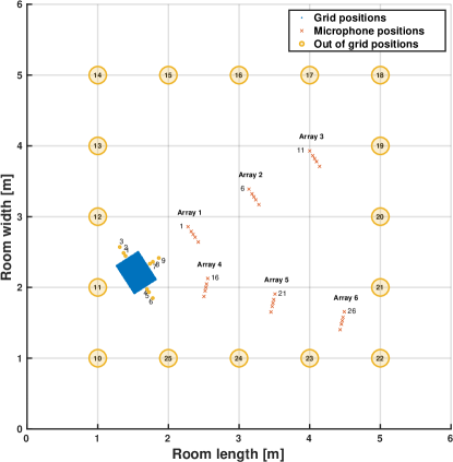
Figure 1: Illustration of the recording setup - Top View.

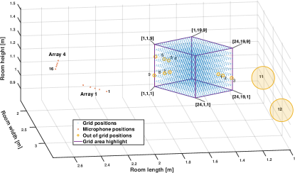
Figure 2: A detailed view of the near area of the grid.

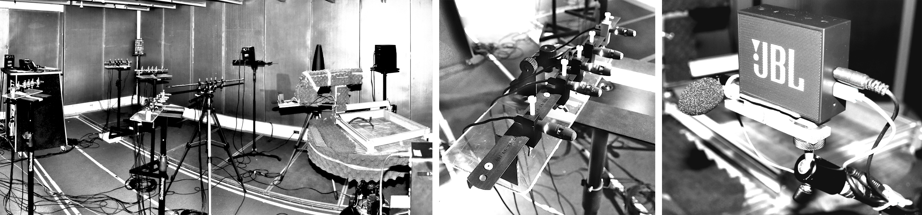
Figure 3: Photos of the recording setup in the acoustic lab. The first photo from left captures the whole room setup with the 3D positioning system and microphones arrays. The second photo shows the microphones array geometry. The third photo shows the loudspeaker located in an OOG position with the mounted microphone.

II-B Realization

The sidewalls and the ceiling of the acoustic lab consist of revolving double-sided panels with a reflecting and an absorbing face. By rotating these panels, the ratio between the reflective and absorbing areas of the room can be modified, by which the reverberation time of the room can be controlled. We have chosen three reverberation time levels: $100$, $300$, and $600$ ms; $T_{60}$ was measured by Brüel & Kjær type 2250 sound level meter employing Brüel & Kjær Omni source loudspeaker type 4295; see examples of RIR Energy Decay Curves in Fig. 5. The other details of the recording hardware are summarized in Table I.

The positioning of the loudspeaker within the grid was realized using a precise three-axis positioning system. It consists of a 2D plotter and a lift table. The $x$ and $y$-axis were controlled automatically by the plotter, while the $z$-axis was operated manually. The height was measured by a laser distance meter mounted to the desk of the table. To attenuate acoustic reflections from the plotter’s rails, a cardboard construction that holds the loudspeaker out of the plotter’s perimeter was constructed (see the first photo in Fig. 3). Positions $10$ through $25$ were measured manually, so the accuracy of their positioning is slightly lower compared that of the positions in the grid.

For each position, two excitation signals were played and recorded in sequence: The first signal (Chirp) consists of two repetitions of a logarithmic swept-frequency cosine signal with a total length of $20$ seconds ($0.5$ s silence, $8$ s chirp, $2$ s silence, $8$ s chirp, $1.5$ s silence). White noise (WN) was used as the second excitation signal with a total length of $10$ seconds ($0.5$s silence, $8$s WN, $1.5$s silence). Due to the limited frequency range of the loudspeaker ($180$ Hz - $20$ kHz), the Chirp signals starts from $200$ Hz through $16$ kHz. To prevent rapid phase changes and subsequent “popping”, all excitation signals were linearly faded in and out over 0.2 seconds.

We have also recorded one hour of room tone (silence) and one hour of diffuse babble noise for each T₆₀ setting. The babble noise was simulated by using eight loudspeakers each playing a different multi-speech sequence and each placed approximately $1$ m from the walls: one in each corner and one in the middle of each wall. The loudspeakers were directed towards the nearest corner or the nearest wall. Four of these loudspeakers can be seen in the first photo in Fig. 3.

TABLE I: Recording equipment

Microphones	AKG CK32
Mic preamp. $+$ AD/DA	ANDIAMO.MC
Loudspeaker (grid, OOG)	JBL Go
Loudspeaker (babble noise)	6301bx Fostex

The recording/playback was done with the sampling frequency of $48$ kHz and the bit rate of $32$ bits per sample. In order to reduce the size of the raw database ($1.5$ TB), all recordings were re-encoded into the FLAC format (Free Lossless Audio Codec) with 48 kHz and 24 bits per sample (50% reduction).

[ template=signpost, level distance=2mm, level size=5mm, ] child gMIRaGe child gDB cWN 100 cWN 300 cWN 600 cChirp 100 cChirp 300 cChirp 600 child gMISC child g100 cBabble cRoomTone child g300 c[id=node_C]Babble cRoomTone child g600 c[id=node_A]Babble cRoomTone

Figure 4: Database directory structure: The acronyms WN and Chirp correspond to the excitation signals as defined in Section II-B. The numbers $100$, $300$, and $600$ correspond to the reverberation time level. MISC contains the recordings of the room tone and of the babble noise.

II-C Database package

The database can be downloaded part-by-part according to the directory structure shown in Fig. 4. Each directory at the bottom level in Fig. 4 comprises seven folders: one per each microphone array (01, …, 06) and one for the microphone mounted to the loudspeaker (on_SPK_mic). A software package for Matlab is available at the same webpage; the software documentation is included. It enables users to compute RIRs and relative RIRs or, equivalently, ATFs or Relative Transfer Functions (RTF) [15] directly from the raw recordings for selected positions, microphones and the other parameters. The entire database has $0.7$ TB (FLAC) in size, however, only selected parts can be downloaded and used with the software.

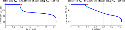
Figure 5: Samples of RIR Energy Decay Curves (EDCs) created from the MIRaGe database (mic 1, position [12,10,5]); $T_{60}$ was estimated from manually selected (marked - red, cyan) linear parts of EDCs

III Using the database: Examples

We will give now two applications that can benefit from this database. The database can be used in many more applications.

Given a pair of microphones $i$ and $j$, their noisy observations of a directional source can be described as

$$x_{i} =s*h_{i}+v_{i},$$ (1)

$$x_{j} =s*h_{i}*g_{i,j}+v_{j},$$

where $x_{i}$ is the observed signal by the $i$th microphone, $i=1,2$, $s$ is the source signal, $h_{i}$ is the room impulse response between the source and the $i$th microphone, $v_{i}$ is the noise signal in the $i$th microphone, and $g_{i,j}$ is the relative impulse response (ReIR) between microphones $i$ and $j$ (reference). It holds that $h_{j}=h_{i}*g_{i,j}$.

The frequency domain counterpart of the ReIR is the Relative Transfer Function (RTF), a term which we will use in the following as it is more frequently used in the literature [15]. An ATF could be seen as a special case of RTF where the non-reference microphone is a virtual one whose output is the original (non-spatial) signal $s$ (then, $h_{i}=\delta$ and $g_{i,j}=h_{j}$). Alternatively, this virtual microphone can be substituted by a microphone that is very close to the source (e.g., microphone 31 in our database).

RTFs are commonly used to construct beamformers, e.g. as a blocking matrix in the Generalized Sidelobe Canceller (GSC) implementation. Higher attenuation of the desired signal (i.e. less signal leakage after blocking) is related to lower distortion at the GSC output [15]. We can therefore use the blocking ability of an RTF as an objective measure of quality. Given an RTF $g$, we define the blocking ability of $g$ for microphones $i$ and $j$ as

$${\rm BA}_{i,j}(g)=-10\log_{10}\left(\frac{{\rm var}[s_{r}]/{\rm var}[v_{r}]}{{\rm var}[s]/{\rm var}[v]}\right)$$ (2)

where ${\rm var}[\cdot]$ stands for the variance of the argument, $s_{r}$ is the residual of $s$ at the output of the blocking operation $x_{i}*g-x_{j}$, that is, $s_{r}=s*h_{i}*g-s*h_{j}$, and, similarly, $v_{r}$ is the residual of the noise, $v_{r}=v_{i}*g-v_{j}$. This measure reflects the attenuation of the source relative to the attenuation of the noise. Ideally, when $g$ corresponds to the exact RTF, i.e. $g=g_{i,j}$, then $s_{r}=0$ and ${\rm BA}_{i,j}(g)=+\infty$.

III-A Experiment 1

In this experiment, we consider grid positions [:,1,1]. The dataset recordings of the white noise for these positions observed by array 1 were taken (microphones 1 through 5). The recordings were used to compute RTFs using time-domain least squares, with microphone 1 being the reference. These positions will be referred to as reference positions.

Then, a source at position [18,1,5] (referred to as test position) is considered. Spatial images of a white noise signal played from the test position were simulated using the relevant ATFs of the database. The ATFs were obtained similarly using the database recordings for the test position by mics 1 through 5 and the original excitation signal.

Now, the blocking ability of the RTFs when considering the source in the test position were computed. Signals were downsampled to 16 kHz. The time-domain length of the ATFs was 7168 taps and that of the RTFs was 1536 taps. $T_{60}$ levels examined were $100$ ms and $600$ ms, respectively. To compare, the entire experiment was also simulated using the RIR generator [16]. The blocking ability of the RTFs averaged over microphones 1 through 5 as a function of the reference position is shown in Fig. 6.

Figure 6: Blocking ability per reference positions.

The results show that the closer the reference position is to the test position (#18), the higher is the blocking ability. With higher reverberation time, the overall blocking ability is lower, which is due to the insufficient time-domain length of the RTFs (1536 taps). The overall trends of the blocking ability for the real and the simulated experiment are similar, nevertheless, the values are different. This shows that the reverberation tails of the RIRs from the laboratory are significantly different from those of the simulated room.

III-B Experiment 2

In [11], a method, denoted manifold projection (MP), for supervised RTF identification was introduced for the purpose of increasing the robustness of optimal beamformers. In this method, a manifold of typical RTFs in a particular room is learned in advance and then exploited to improve the identification of unknown RTFs based on noisy measurements. The method was evaluated in [11] only using a simulated experiment and was shown to provide superior blocking ability over the noisy measurement-based RTF, especially in low SNR conditions. In our experiments, we evaluate the performance of this method in realistic conditions using our database.

First, we repeated the experimental setup in [11] as closely as possible with our database. We used every second position in the grid’s $x$-axis, every position of the $z$-axis and the first position of the $y$-axis (i.e. [1:2:24,1,:], for a total of $12\times 1\times 9$ positions). For each of these positions, the RTF was calculated between microphones 14 and 15 (Array 3, $8$ cm inter-mic distance, $3$ m in front of the grid) using clean excitation white noise signals. These RTFs serve as the training set in the supervised methods. The same setup was also created using the RIR simulator.

In one trial of the experiment, a new position within the grid except any positions in [:,1,:] is randomly selected. A 3-second long speech signal is simulated from that position. An uncorrelated spatial white noise at different signal-to-noise ratio (SNR) levels is added. From the noisy mixture, an RTF is estimated using the frequency-domain estimator proposed by Gannot et al. [15]. This noisy RTF estimate is then compared to the training RTFs using the Euclidian distance, and the closest RTF is chosen in place of the noisy one. This approach is referred to as Nearest Neighbor (NN). To compare, the noisy RTF estimate is also enhanced using MP [11]. The resulting RTF estimates were evaluated using the blocking ability with respect to the simulated source. The other parameters were the same as in the first experiment. The average results of 1000 independent trials are shown in Fig. 7.

Figure 7: Results of the second experiment

The results show that both supervised methods provide superior blocking ability compared to the unsupervised method (the noisy RTF estimate) when the input SNR is lower than $0$ dB or $-10$ dB, depending on the reverberation time. While both NN and MP methods perform similarly in the simulated conditions and low reverberation time, MP provides consistently better results than NN in terms of the blocking ability when using real data.

IV Conclusions

We have introduced a new database of dense measurements within a 3D area of an acoustic lab. We have shown that the database can be used for detailed analyses of spatial processing algorithms subject to source location within the measured area. Small variations of RIRs and ReIRs (resp. ATFs and RTFs) due to small changes of the source location can be observed. The database provides an alternative to the popular room impulse response simulator based on the image method [1, 16].

Appendix: MIRaGe utilities screenshots

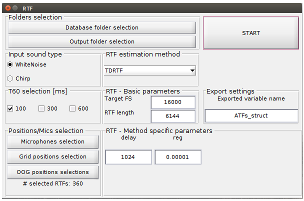
Figure 8: Main window

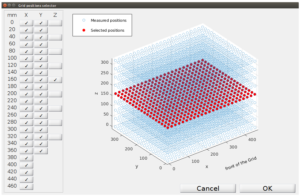
Figure 9: Grid positions selection window

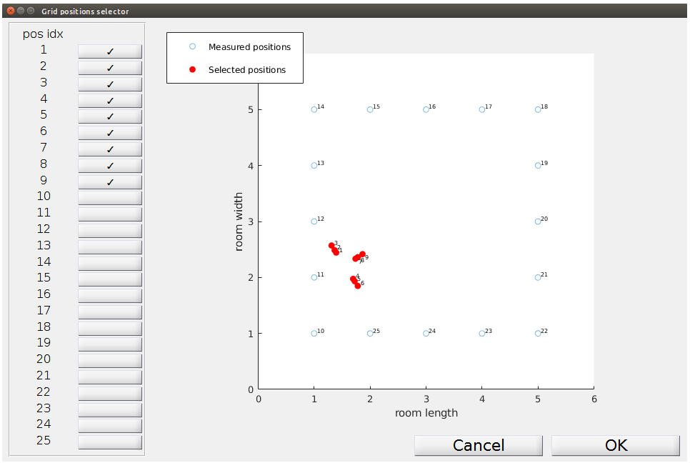
Figure 10: Out-Of-Grid positions selection window

Figure 11: Microphones selection window

References

- [1] J. B. Allen and D. A. Berkley, “Image method for efficiently simulating small‐room acoustics,” The Journal of the Acoustical Society of America, vol. 65, no. 4, pp. 943–950, 1979.
- [2] M. Jeub, M. Schafer, and P. Vary, “A binaural room impulse response database for the evaluation of dereverberation algorithms,” in 2009 16th International Conference on Digital Signal Processing, July 2009, pp. 1–5.
- [3] H. Kayser, S. D. Ewert, J. Anemüller, T. Rohdenburg, V. Hohmann, and B. Kollmeier, “Database of multichannel in-ear and behind-the-ear head-related and binaural room impulse responses,” EURASIP Journal on Advances in Signal Processing, vol. 2009, no. 1, p. 298605, Jul 2009.
- [4] R. Stewart and M. Sandler, “Database of omnidirectional and b-format room impulse responses,” in 2010 IEEE International Conference on Acoustics, Speech and Signal Processing, March 2010, pp. 165–168.
- [5] E. Hadad, F. Heese, P. Vary, and S. Gannot, “Multichannel audio database in various acoustic environments,” in 2014 14th International Workshop on Acoustic Signal Enhancement (IWAENC), Sep. 2014, pp. 313–317.
- [6] Y. R. Zheng, R. A. Goubran, and M. El-Tanany, “Robust near-field adaptive beamforming with distance discrimination,” IEEE Transactions on Speech and Audio Processing, vol. 12, no. 5, pp. 478–488, Sep. 2004.
- [7] A. Barnov, V. B. Bracha, S. Markovich-Golan, and S. Gannot, “Spatially robust gsc beamforming with controlled white noise gain,” in 2018 16th International Workshop on Acoustic Signal Enhancement (IWAENC), Sep. 2018, pp. 231–235.
- [8] M. Fakhry and F. Nesta, “Underdetermined source detection and separation using a normalized multichannel spatial dictionary,” in IWAENC 2012; International Workshop on Acoustic Signal Enhancement, Sep. 2012, pp. 1–4.
- [9] Z. Koldovský, J. Málek, P. Tichavský, and F. Nesta, “Semi-blind noise extraction using partially known position of the target source,” IEEE Transactions on Audio, Speech, and Language Processing, vol. 21, no. 10, pp. 2029–2041, Oct 2013.
- [10] E. Weinstein, K. Steele, A. Agarwal, and J. Glass, “LOUD: A 1020-node microphone array and acoustic beamformer,” in 14th International Congress on Sound and Vibration (ICSV), July 2007.
- [11] R. Talmon and S. Gannot, “Relative transfer function identification on manifolds for supervised GSC beamformers,” in 21st European Signal Processing Conference (EUSIPCO 2013). IEEE, 2013, pp. 1–5.
- [12] B. Laufer-Goldshtein, R. Talmon, and S. Gannot, “A study on manifolds of acoustic responses,” in Latent Variable Analysis and Signal Separation, E. Vincent, A. Yeredor, Z. Koldovský, and P. Tichavský, Eds. Cham: Springer International Publishing, 2015, pp. 203–210.
- [13] B. Laufer-Goldshtein, R. Talmon, and S. Gannot, “A real-life experimental study on semi-supervised source localization based on manifold regularization,” in 2016 IEEE International Conference on the Science of Electrical Engineering (ICSEE), Nov 2016, pp. 1–5.
- [14] F. Katzberg, R. Mazur, M. Maass, P. Koch, and A. Mertins, “A compressed sensing framework for dynamic sound-field measurements,” IEEE/ACM Transactions on Audio, Speech, and Language Processing, vol. 26, no. 11, pp. 1962–1975, Nov 2018.
- [15] S. Gannot, D. Burshtein, and E. Weinstein, “Signal enhancement using beamforming and nonstationarity with applications to speech,” IEEE Transactions on Signal Processing, vol. 49, no. 8, pp. 1614–1626, Aug 2001.
- [16] E. A. Habets, “Room impulse response generator,” Technische Universiteit Eindhoven, Tech. Rep, vol. 2, no. 2.4, 2006.