Quadruply Stochastic Gradients for Large Scale Nonlinear
Semi-Supervised AUC Optimization

Abstract

Semi-supervised learning is pervasive in real-world applications, where only a few labeled data are available and large amounts of instances remain unlabeled. Since AUC is an important model evaluation metric in classification, directly optimizing AUC in semi-supervised learning scenario has drawn much attention in the machine learning community. Recently, it has been shown that one could find an unbiased solution for the semi-supervised AUC maximization problem without knowing the class prior distribution. However, this method is hardly scalable for nonlinear classification problems with kernels. To address this problem, in this paper, we propose a novel scalable quadruply stochastic gradient algorithm (QSG-S2AUC) for nonlinear semi-supervised AUC optimization. In each iteration of the stochastic optimization process, our method randomly samples a positive instance, a negative instance, an unlabeled instance and their random features to compute the gradient and then update the model by using this quadruply stochastic gradient to approach the optimal solution. More importantly, we prove that QSG-S2AUC can converge to the optimal solution in $O(1/t)$, where $t$ is the iteration number. Extensive experimental results on a variety of benchmark datasets show that QSG-S2AUC is far more efficient than the existing state-of-the-art algorithms for semi-supervised AUC maximization, while retaining the similar generalization performance.

1 Introduction

Semi-supervised learning addresses the problems where the available data is composed of a small size of labeled samples and a huge size of unlabeled samples. It is of immense practical interest in a wide range of applications, such as image retrieval  Wang et al. (2010), natural language processing  Liang (2005) and speech analysis  Sholokhov et al. (2018). Since semi-supervised learning requires less human effort and can achieve a better generalization performance, it has attracted a great deal of attention in the machine learning communities, i.e.,  Gu et al. (2018c); Sakai et al. (2017, 2018); Geng et al. (2019); Yu et al. (2019).

The area under the ROC curve (AUC)  Hanley and McNeil (1982) measures the probability of a randomly drawn positive instance being ranked higher than a randomly drawn negative instance. Thus, AUC is a more effective performance measure than the accuracy in data imbalance binary classification problem. Many studies  Gao et al. (2013); Gao and Zhou (2015) have also pointed out that optimizing AUC can achieve a better generalization performance than directly optimizing accuracy. Due to the superiority of AUC as mentioned above, a large amount of attention has been attracted to introduce AUC to semi-supervised learning.

Recently, several algorithms have been proposed to address the semi-supervised AUC optimization problem. For instance, to train a classifier, SSRankBoost  Amini et al. (2008) and OptAG  Fujino and Ueda (2016) exploited the assumption that two samples share the same label if their distance in a metric space is small. However, this restrictive assumption may not always hold in real-world applications, and could lead to biased solutions. Sakai et al., Sakai et al. (2018) pointed out that both unlabeled instances and labeled instances follow the same joint probability distribution and the restrictive assumption is not necessary. However, their method PNU-AUC requires to estimate the class prior which is difficult to be obtained when labeled instances are extremely small. Recently, Xie and Li, Xie and Li (2018) proposed that neither the class priors nor any other distributional assumption about the unlabeled data are necessary to find the unbiased solution. We summarize these algorithms in Table 1.

Algorithm	Reference	Function model	Computational complexity	Space complexity
SSRankBoost	Amini et al. (2008)	Nonlinear model	—	$O(n^{2})$
OptAG	Fujino and Ueda (2016)	Linear model	—	$O(n^{2})$
PNU-AUC	Sakai et al. (2018)	Nonlinear model	$O(n^{3})$	$O(n^{2})$
SAMULT	Xie and Li (2018)	Nonlinear model	$O(n^{3})$	$O(n^{2})$
QSG-S2AUC	Ours	Nonlinear model	$O(Dt^{2})$	$O(t)$

Table 1: Several representative semi-supervised AUC optimization algorithms. ($D$ denotes the number of random features, $n$ denotes the number of training samples and $t$ denotes number of iterations.)

Nonlinear data structures widely exist in many real-world problems, and kernel method is a typical way to solve such problems Huang et al. (2019); Gu et al. (2014). However, this approach can hardly scale to large datasets. Specifically, the kernel matrix needs $O(n^{2}d)$ operations to be calculated and $O(n^{2})$ to be stored, where $n$ denotes the number of instances and $d$ denotes the dimensionality of the data  Gu and Huo (2018). However, the bottlenecks of the computational complexities become more severe for semi supervised learning because the sample size $n$ is always very large in the semi-supervised scenario. Even worse, PNU-AUC and SAMULT  Xie and Li (2018) need $O(n^{3})$ operations to compute the matrix inverse. Thus, scaling up non-linear semi-supervised AUC maximization is a challenging problem.

To scale up kernel-based algorithms, a large amount of methods has been proposed, i.e., asynchronous parallel algorithms  Gu et al. (2018a); Gu and Huo (2018); Gu et al. (2016), kernel approximation  Rahimi and Recht (2008); Smola and Schölkopf (2000). To our knowledge, doubly stochastic gradient (DSG)  Dai et al. (2014) is the most effective method to scale up kernel-based algorithms. Specifically, DSG samples a random instance and the random features to compute the doubly stochastic gradient which is used to update the model. However, different from the standard DSG, semi-supervised learning has three sources of data, i.e., positive instances, negative instances and unlabeled datasets. In addition, optimizing AUC is a pairwise learning problem which is more complicated than the pointwise learning problem considered in the standard DSG algorithm. Therefore, the existing algorithms and theoretical analysis for DSG cannot be directly applied to non-linear semi-supervised AUC maximization.

To address this challenging problem, we introduce multiple sources of randomness. Specifically, we randomly sample a positive, a negative and an unlabeled instance in each iteration to compose a triplet of data points. Then we use the random features w.r.t these data triplets to compute the stochastic gradient. Since the stochastic gradient would then contain four sources of randomness, we denote our algorithm as quadruply stochastic semi-supervised AUC maximization (QSG-S2AUC). Theoretically, we prove that QSG-S2AUC can converge to the optimal solution at the rate of $O(1/t)$, where $t$ is the number of gradient iterations. Extensive experimental results on a variety of benchmark datasets show that QSG-S2AUC is far more efficient than the existing state-of-the-art algorithms for semi-supervised AUC maximization, while retaining the similar generalization performance.

Contributions. The main contributions of this paper are summarized as follows.

1. We propose an efficient nonlinear semi-supervised AUC optimization algorithm based on the DSG framework. Since semi-supervised learning contains three sources of data, we employ triplets of data points in each iteration and extend the standard DSG framework.

2. We prove that QSG-S2AUC has the convergence rate of $O(1/t)$ which is same to the one of standard SGD even though our QSG-S2AUC has four sources of randomness.

2 Related Works

In this section, we give a brief review of kernel approximation and large scale AUC maximization methods respectively.

2.1 Kernel Approximation

Kernel approximation has attracted great amounts of attention to scale up kernel-based learning algorithms. The data-dependent methods, such as greedy basis selection techniques  Smola and Schölkopf (2000), incomplete Cholesky decomposition  Fine and Scheinberg (2001), Nyström method  Drineas and Mahoney (2005), utilize the given training set to compute a low-rank approximation of the kernel matrix. However, they need a large amount of training instances to achieve a better generalization. To handle this challenge, random Fourier feature (RFF)  Rahimi and Recht (2008) directly approximates the kernel function unbiasedly with some basis functions. However, large amounts of memory are required since the number random features $D$ need to be larger than the original features to achieve low approximation error. To further improve RFF, Dai et al., Dai et al. (2014) proposed DSG algorithm. It uses pseudo-random number generators to calculate the random features on-the-fly, which highly reduces the memory requirement. These methods have been widely applyed to scale up kernel-based learning algorithms, such as  Li et al. (2017); Gu et al. (2018b).

2.2 Large Scale AUC Optimization

Recently, several efforts have been devoted to scale up the AUC optimization. For example, Ying et al., Ying et al. (2016) formulated the AUC optimization as a convex-concave saddle point problem and proposed a stochastic online method (SOLAM) which has the time and space complexities of one datum. FSAUC  Liu et al. (2018) developed a multi-stage scheme for running primal-dual stochastic gradient method with adaptively changing parameters. FSAUC has the convergence rate of $O(1/n)$, where $n$ is the number of random samples. However, both SOLAM and FSAUC focus on scaling up the linear AUC optimization and are incapable of maximizing AUC in the nonlinear setting. Recently, FOAM and NOAM  Ding et al. (2017) used RFF and Nyström method, respectively, to scale up the kernel based AUC optimization problem. However, as mentioned above, both methods require large amounts of memory to achieve a better generalization performance and not trivial to scale up the nonlinear semi-supervised AUC optimization problems based.

3 Preliminaries

3.1 Supervised AUC Optimization

In supervised learning, let $x\in\mathbb{R}^{d}$ be a $d$-dimensional pattern and $y\in\{+1,-1\}$ be a class label. Let $p(x,y)$ be the underlying joint density of $(x,y)$. The $\mathrm{AUC}$ optimization is to train a classifier $f$ that maximizes the following function.

$$\mathrm{AUC} = 1-\mathbb{E}_{x^{p}\sim p^{+}(x)}\left[\mathbb{E}_{x^{n}\sim p^{-}(x)}[l_{01}(f(x^{p}),f(x^{n}))]\right],$$

where $p^{+}(x)=p(x|y=+1)$, $p^{-}(x)=p(x|y=-1)$ and $l_{01}(u,v)=(1-\mathrm{sign}(u-v))/2$. Obviously, maximizing AUC is equivalent to minimizing the following PN AUC risk.

$$R_{\mathrm{PN}} =\mathbb{E}_{x^{p}\sim p^{+}(x)}\left[\mathbb{E}_{x^{n}\sim p^{-}(x)}[l_{01}(f(x^{p}),f(x^{n}))]\right].$$ (1)

Given the positive and negative datasets as $D_{p}=\{x_{i}\}_{i=1}^{p}\sim p^{+}(x)$ and $D_{n}=\{x_{j}\}_{j=1}^{n}\sim p^{-}(x)$ respectively. Thus, the PN AUC risk can be rewritten as follows.

$$R_{\mathrm{PN}} =\mathbb{E}_{x^{p}\in D_{p}}\left[\mathbb{E}_{x^{n}\in D_{n}}[l(f(x^{p}),f(x^{n}))]\right].$$ (2)

where $\mathbb{E}_{x^{p}\in D_{p}}$ and $\mathbb{E}_{x^{n}\in D_{n}}$ denote the means of $D_{p}$ and $D_{n}$, respectively.

3.2 Semi-Supervised AUC Optimization

Since large amounts of instances remain unlabeled in semi-supervised learning, we assume that the labeled dataset is limited while the unlabeled data can be infinite and has the underlying distribution density of $p(x)$, where $p(x)=\pi p^{+}(x)+(1-\pi)p^{-}(x)$ and $\pi$ denotes the positive class prior. Recently, Xie and Li, Xie and Li (2018) have shown that it is unnecessary to estimate distributional assumptions or class prior to achieve an unbiased solution for semi-supervised AUC optimization. Specifically, PU AUC risk $R_{\mathrm{PU}}$ and NU AUC risk $R_{\mathrm{NU}}$ are equivalent to the supervised PN AUC risk $R_{\mathrm{PN}}$ risk with a linear transformation, where PU AUC risk $R_{\mathrm{PU}}$ is estimated by positive and unlabeled data treated as negative data, and NU AUC risk $R_{\mathrm{NU}}$ is estimated by negative and unlabeled data treated as positive data. We define $R_{\mathrm{PU}}$ and $R_{\mathrm{NU}}$ as follows,

$$R_{\mathrm{PU}} = \mathbb{E}_{x^{p}\in D_{p}}\left[\mathbb{E}_{x^{u}\sim p(x)}[l(f(x^{p}),f(x^{u}))]\right],$$ (3)

$$R_{\mathrm{NU}} = \mathbb{E}_{x^{u}\sim p(x)}\left[\mathbb{E}_{x^{n}\in D_{n}}[l(f(x^{u}),f(x^{n}))]\right],$$ (4)

where $\mathbb{E}_{x^{u}\sim p(x)}$ denotes the expectation over the density $p(x)$. PU AUC risk can be written as follows.

$$R_{\mathrm{PU}}= \mathbb{E}_{x^{p}\in D_{p}}[\mathbb{E}_{x^{u}\sim p(x)}[l(f(x^{p}),f(x^{u}))]]$$

$$= \mathbb{E}_{x^{p}\in D_{p}}[\pi\mathbb{E}_{x^{\prime p}\sim p^{+}(x)}[l(f(x^{p},x^{\prime p}))]$$

$$+(1-\pi)\mathbb{E}_{x^{\prime n}\sim p^{-}(x)}[l(f(x^{p},x^{\prime n}))]]$$

$$= \dfrac{1}{2}\pi+(1-\pi)R_{\mathrm{PN}},$$ (5)

where $x^{\prime p}$ and $x^{\prime n}$ denotes the positive and negative instances in unlabeled dataset. Similarly, NU AUC risk $R_{\mathrm{NU}}$ can be rewritten as

$$R_{\mathrm{NU}}=\dfrac{1}{2}(1-\pi)+\pi R_{\mathrm{PN}}.$$ (6)

Then PN AUC risk $R_{\mathrm{PN}}$ can be formulated as follows.

$$R_{\mathrm{PU}}+R_{\mathrm{NU}}-\dfrac{1}{2}=R_{\mathrm{PN}}.$$ (7)

Thus, the semi-supervised AUC optimization can be formulated as follows.

$$R_{\mathrm{PNU}}=(1-\gamma)\left(R_{\mathrm{PU}}+R_{\mathrm{NU}}-\dfrac{1}{2}\right)+\gamma R_{\mathrm{PN}}.$$ (8)

where $\gamma\in[0,1]$ is the trade-off parameter. To reduce the risk of overfitting, we add a $l_{2}$-regularizer into (8) and have the following objective for semi-supervised AUC optimization.

$$\mathcal{L}=R_{\mathrm{PNU}}(f)+\dfrac{\lambda}{2}\|f\|_{\mathcal{H}}^{2},$$ (9)

where $\lambda$ is the regularized parameter and $\|\cdot\|_{\mathcal{H}}$ denotes the norm in a reproducing kernel Hilbert space (RKHS) $\mathcal{H}$.

3.3 Random Fourier Feature

In this section, we give a brief review of RFF. Assume that we have a continuous, real-valued, symmetric and shift-invariant kernel function $k(x,x^{\prime})$. According to Bochner Theorem  Rudin (2017), this kernel function is positive definite and has a nonnegative Fourier transform function as $k(x,x^{\prime})=\int_{\mathbb{R}^{d}}p(\omega)e^{j\omega^{T}(x-x^{\prime})}d\omega$, where $p(w)$ is a density function associated with $k(x,x^{\prime})$. The integrand $e^{j\omega^{T}(x-x^{\prime})}$ can be replaced with $\cos\omega^{T}(x-x^{\prime})$  Rahimi and Recht (2008). Then we can obtain a real-valued feature map $\phi_{\omega_{i}}(x)=[\cos(\omega_{i}^{T}x),\sin(\omega_{i}^{T}x)]^{T}$, where $\omega_{i}$ is randomly sampled according to the density function $p(\omega)$. We can obtain the feature map for $m$ random features of a real-valued kernel as follows.

$$\phi_{\omega}(x)=\sqrt{1/D}[\cos(\omega_{1}^{T}x),\cdots,\cos(\omega_{m}^{T}x),$$

$$\sin(\omega_{1}^{T}x),\cdots,\sin(\omega_{m}^{T}x)]^{T}.$$ (10)

Obviously, $\phi^{T}_{\omega}(x)\phi_{\omega}(x^{\prime})$ is an unbiased estimate of $k(x-x^{\prime})$.

4 Quadruply Stochastic Semi-Supervised AUC Maximization

4.1 Quadruply Stochastic Gradients

Based on the definition of the function $f\in\mathcal{H}$, we easily obtain $\nabla f(x)=\nabla\langle f,k(x,\cdot)\rangle$, and $\nabla\|f\|_{\mathcal{H}}^{2}=\nabla\langle f,f\rangle_{\mathcal{H}}=2f$. Thus, the gradient of the objective (9) can be written as:

$$\nabla\mathcal{L}= \lambda f+\gamma\mathbb{E}_{x^{p}\in D_{p}}[\mathbb{E}_{x^{n}\in D_{n}}[l_{1}^{\prime}k(x^{p},\cdot)+l_{2}^{\prime}k(x^{n},\cdot)]]$$

$$+(1-\gamma)(\mathbb{E}_{x^{p}\in D_{p}}[\mathbb{E}_{x^{u}\sim p(x)}[l_{3}^{\prime}k(x^{p},\cdot)+l_{4}^{\prime}k(x^{u},\cdot)]]$$

$$+\mathbb{E}_{x^{u}\sim p(x)}[\mathbb{E}_{x^{n}\in D_{n}}[l_{5}^{\prime}k(x^{u},\cdot)+l_{6}^{\prime}k(x^{n},\cdot)]]),$$ (11)

where $l_{1}^{\prime}k(x^{p},\cdot)$ denotes the derivative of $l(f(x^{p}),f(x^{n}))$ w.r.t. $f(x^{p})$, $l_{2}^{\prime}k(x^{n},\cdot)$ denotes the derivative of $l(f(x^{p}),f(x^{n}))$ w.r.t. $f(x^{n})$, $l_{3}^{\prime}k(x^{p},\cdot)$ denotes the derivative of $l(f(x^{p}),f(x^{u}))$ w.r.t. $f(x^{p})$, $l_{4}^{\prime}k(x^{u},\cdot)$ denotes the derivative of $l(f(x^{p}),f(x^{u}))$ w.r.t. $f(x^{u})$, $l_{5}^{\prime}k(x^{u},\cdot)$ denotes the derivative of $l(f(x^{u}),f(x^{n}))$ w.r.t. $f(x^{u})$ and $l_{6}^{\prime}k(x^{n},\cdot)$ denotes the derivative of $l(f(x^{u}),f(x^{n}))$ w.r.t. $f(x^{n})$.

In order to update the classifier $f$ in a stochastic manner,we randomly sample a positive data point $x^{p}$ and a negative data point $x^{n}$ from $D_{p}$ and $D_{n}$, respectively. In addition, we randomly sample an unlabeled data point $x^{u}$ according to the unlabeled data distribution density $p(x)$. In each iteration, we use a triplet of these data points to compute the stochastic functional gradient of (8) as follows.

$$\xi(\cdot)= \gamma(l_{1}^{\prime}k(x^{p},\cdot)+l_{2}^{\prime}k(x^{n},\cdot))+(1-\gamma)(l_{3}^{\prime}k(x^{p},\cdot)$$

$$+l_{4}^{\prime}k(x^{u},\cdot)+l_{5}^{\prime}k(x^{u},\cdot)+l_{6}^{\prime}k(x^{n},\cdot)).$$ (12)

We can apply the random Fourier feature method to further approximate the stochastic functional gradient $\xi(\cdot)$ as follows.

$$\zeta(\cdot)= \gamma(l_{1}^{\prime}\phi_{\omega}(x^{p})\phi_{\omega}(\cdot)+l_{2}^{\prime}\phi_{\omega}(x^{n})\phi_{\omega}(\cdot))$$

$$+(1-\gamma)(l_{3}^{\prime}\phi_{\omega}(x^{p})\phi_{\omega}(\cdot)+l_{4}^{\prime}\phi_{\omega}(x^{u})\phi_{\omega}(\cdot)$$

$$+l_{5}^{\prime}\phi_{\omega}(x^{u})\phi_{\omega}(\cdot)+l_{6}^{\prime}\phi_{\omega}(x^{n})\phi_{\omega}(\cdot)).$$ (13)

Obviously, we have that $\xi(\cdot)=\mathbb{E}_{\omega}[\zeta(\cdot)]$. Thus, we can achieve the unbiased estimate of the gradient (4.1) by using either $\xi(\cdot)$ or $\zeta(\cdot)$ as follows,

$$\nabla\mathcal{L}=\mathbb{E}_{x^{p},x^{n},x^{u}}[\xi(\cdot)]+\lambda f,\nabla\mathcal{L}=\mathbb{E}_{x^{p},x^{n},x^{u}}[\mathbb{E}_{\omega}[\zeta(\cdot)]]+\lambda f.$$

Because four randomness (i.e. $x^{p}$, $x^{n}$, $x^{u}$ and $\omega$) are involved in $\zeta(\cdot)$, we call the functional gradient $\zeta(\cdot)$ as quadruply stochastic functional gradient.

Then, we first give the update rule with the stochastic gradient $\xi(\cdot)$ as follow,

$$h_{t+1}(\cdot)=h_{t}(\cdot)-\eta_{t}\left(\xi_{t}(\cdot)+\lambda h_{t}(\cdot)\right)=\sum_{i=1}^{t}a_{t}^{i}\xi_{t}(\cdot),\ \ \forall t>1,$$

where $\mathit{a}_{t}^{i}=-\eta_{t}\prod_{j=i+1}^{t}(1-\eta_{j}\lambda)$, $\eta_{t}$ denotes the step size and $h_{t+1}(x)$ denotes the function value if we use gradient $\xi(\cdot)$. Since $\zeta(\cdot)$ is an unbiased estimate of $\xi(\cdot)$, the update rule using $\zeta(\cdot)$ after $t$ iterations can be written as follow,

$$f_{t+1}(\cdot) =f_{t}(\cdot)-\eta_{t}\left(\zeta_{t}(\cdot)+\lambda f_{t}(\cdot)\right)=\sum_{i=1}^{t}a_{t}^{i}\zeta_{i}(\cdot),\quad\forall t>1,$$

where $f_{1}(\cdot)=0$, and $f_{t+1}(x)$ denotes the function value for the input $x$ if we use the functional gradient $\zeta(\cdot)$.

In order to implement the update process in computer program, we rewrite the update rule as the following iterative update rules with constantly-changing coefficients $\{\alpha_{i}\}_{i=1}^{t}$,

$$f_{t} = \sum_{i=1}^{t}\alpha_{i}\phi_{\omega}(x),$$ (14)

$$\alpha_{i} = -\eta_{i}(\gamma(l_{1}^{\prime}\phi_{\omega}(x^{p})+l_{2}^{\prime}\phi_{\omega}(x^{n}))$$ (15)

$$+(1-\gamma)(l_{3}^{\prime}\phi_{\omega}(x^{p})+l_{4}^{\prime}\phi_{\omega}(x^{u})$$

$$+l_{5}^{\prime}\phi_{\omega}(x^{u})+l_{6}^{\prime}\phi_{\omega}(x^{n}))),$$

$$\alpha_{j} = (1-\eta_{j}\lambda)\alpha_{j},\;\mathrm{for}\;j=1,...,i-1.$$ (16)

Algorithm 1 $\{\alpha_{i}\}_{i=1}^{t}$ = QSG-S2AUC$(D_{p},D_{n},p(x))$

0:  $p(\omega)$, $\phi_{\omega}(x)$, $l(u,v)$, $\lambda$.

0:  $\{\alpha_{i}\}_{i=1}^{t}$

1:  for $i=1,...,t$ do

2:     Sample $x^{p}$ from $D_{p}$.

3:     Sample $x^{n}$ from $D_{n}$.

4:     Sample $x^{u}\sim p(x)$.

5:     Sample $\omega_{i}\sim p(\omega)$ with seed $i$.

6:     $f(x_{i})=$ Predict$(x_{i},\{\alpha_{i}\}_{j=1}^{i-1})$.

7:     $\alpha_{i}=-\eta_{i}(\gamma(l_{1}^{\prime}\phi_{\omega}(x^{p})+l_{2}^{\prime}\phi_{\omega}(x^{n}))+(1-\gamma)(l_{3}^{\prime}\phi_{\omega}(x^{p})+l_{4}^{\prime}\phi_{\omega}(x^{u})+l_{5}^{\prime}\phi_{\omega}(x^{u})+l_{6}^{\prime}\phi_{\omega}(x^{n})))$

8:     $\alpha_{j}=(1-\eta_{j}\lambda)\alpha_{j}\;for\;j=1,...,i-1$.

9:  end for

Algorithm 2 $f(x)=$Predict$(x,\{\alpha_{i}\}_{i=1}^{t})$

0:  $p(\omega),\phi_{\omega}(x)$

0:  $f(x)$

1:  Set $f(x)=0$.

2:  for $i=1,...,t$ do

3:     Sample $\omega_{i}\sim p(\omega)$ with seed $i$.

4:     $f(x)=f(x)+\alpha_{i}\phi_{\omega}(x)$

5:  end for

4.2 QSG-S2AUC Algorithms

In our implementation, we use pseudo-random number generators with seed $i$ to sample random features. In each iteration, we only need to keep the seed $i$ aligned between prediction and training. Then the prediction function $f(x)$ can be restored much more easily. Besides, the QSG-S2AUC maintains a sequence of $\{\alpha_{i}\}_{i=1}^{t}$ at each ieration which has low memory requirement. Specifically, each iteration of the training algorithm executes the following steps.

1. Select Random Data Triplets:  Randomly sample a positive instance, a negative instance and an unlabeled instance to compose a data triplet. In addition, we use mini-batch of these data points to achieve a better efficiency.

2. Approximate the Kernel Function:  Sample $\omega_{i}\sim p(\omega)$ with random seed $i$ to calculate the random features on-the-fly. We keep this seed aligned between prediction and training to speed up computing $f(x_{i})=\sum_{i=1}^{t}\alpha_{i}\phi_{\omega}(x)$.

3. Update Coefficients:   We compute the current coefficient $\alpha_{i}$ in $i$-th loop and then update the former coefficients $\alpha_{j}$ for $j=1,\cdots,i-1$ according to the update rule (15) and (16), respectively.

We summarize the algorithms for training and prediction in Algorithm 1 and 2 respectively.

5 Convergence Analysis

In this section, we prove that QSG-S2AUC converges to the optimal solution at the rate of $O(1/t)$. We first give several assumptions which are standard in DSG  Dai et al. (2014).

Assumption 1

(Bound of kernel function). The kernel function is bounded, i.e., $k(x,x^{\prime})\leq\kappa$, where $\kappa>0$.

Assumption 2

(Bound of random feature norm). The random feature norms are bounded, i.e., $|\phi_{\omega}(x)\phi_{\omega}(x^{\prime})|\leq\phi$.

Assumption 3

(Lipschitz continuous). The first order derivation of $l(f(x^{p}),f(x^{n}))$ is $L_{1}$-Lipschitz continuous in terms of $f(x^{p})$ and $L_{2}$-Lipschitz continuous in terms of $f(x^{n})$. Similarly, the first order derivation of $l(f(x^{p}),f(x^{u}))$ is $L_{3}$-Lipschitz continuous in terms of $f(x^{p})$ and $L_{4}$-Lipschitz continuous in terms of $f(x^{u})$ and the first order derivation of $l(f(x^{u}),f(x^{n}))$ is $L_{5}$-Lipschitz continuous in terms of $f(x^{u})$ and $L_{6}$-Lipschitz continuous in terms of $f(x^{n})$.

Assumption 4

(Bound of derivation). There exists $M_{1}>0$, $M_{2}>0$, $M_{3}>0$, $M_{4}>0$, $M_{5}>0$ and $M_{6}>0$, such that $|l_{1}^{\prime}|\leq M_{1}$, $|l_{2}^{\prime}|\leq M_{2}$, $|l_{3}^{\prime}|\leq M_{3}$, $|l_{4}^{\prime}|\leq M_{4}$, $|l_{5}^{\prime}|\leq M_{5}$, $|l_{6}^{\prime}|\leq M_{6}$,

We use the framework of  Dai et al. (2014) to prove that $f_{t+1}$ can converge to the optimal solution $f^{*}$. Specifically, we use the aforementioned $h_{t+1}$ as an intermediate value to decompose the difference between $f_{t+1}$ and $f^{*}$ as follows,

$$|f_{t+1}(x)-f^{*}(x)|^{2}$$ (17)

$$\leq 2\underbrace{|f_{t+1}(x)-h_{t+1}(x)|^{2}}_{\rm error\;due\;to\;random\;features}+2\kappa\underbrace{\|h_{t+1}-f^{*}\|_{\mathcal{H}}.}_{\rm error\;due\;to\;random\;data}.$$

In other words, the total approximation error includes the error caused by approximating the kernel with random features, and the error caused by sampling random data. Finally, the boundary of the original error can be obtained by summing up the boundary of these two parts.

We first give the convergence of error due to random features and random data in Lemmas 1 and 3 respectively. All the detailed proofs are provided in our Appendix.

Lemma 1 (Error due to random features)

Let $\chi$ denotes the whole training set in semi-supervised learning problem. For any $x\in\chi$, we have

$$\mathbb{E}_{x_{t}^{p},x_{t}^{n},x_{t}^{u},\omega}[|f_{t+1}(x)-h_{t+1}(x)|^{2}]\leq B^{2}_{1,t+1},$$ (18)

where $B^{2}_{1,t+1}:=M^{2}(\kappa+\phi)^{2}\sum_{i=1}^{t}|a_{t}^{i}|^{2}$, $B_{1,1}=0$ and $M=\gamma(M_{1}+M_{2})+(1-\gamma)(M_{3}+M_{4}+M_{5}+M_{6})$.

Obviously, the upper bound $B^{2}_{1,t+1}$ depends on the convergence of $|a_{t}^{i}|$, which is given in Lemma 2.

Lemma 2

Suppose $\eta_{i}=\dfrac{\theta}{i}$ ($1\leq i\leq t$) and $\theta\lambda\in(1,2)\cup\mathbb{Z}_{+}$. We have $|a_{t}^{i}|\leq\dfrac{\theta}{t}$ and $\sum_{i=1}^{t}|a_{t}^{i}|^{2}\leq\dfrac{\theta^{2}}{t}$.

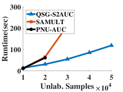
(a) CodRNA

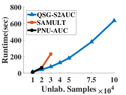
(b) Covtype

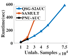
(c) Dota2

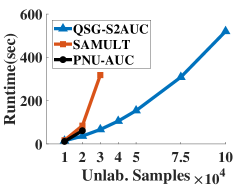
(d) Higgs

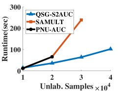
(e) IJCNN1

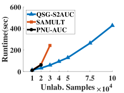
(f) Skin

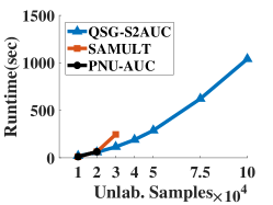
(g) Unclonable

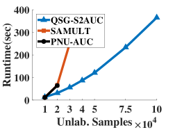
(h) SUSY

Figure 1: The training time of QSG-S2AUC, SAMULT and PNU-AUC against different sizes of unlabeled samples, where the sizes of labeled samples are fixed at 200. (The lines of SAMULT and PNU-AUC are incomplete because their implementations crash on larger training sets.)

Dataset	Features	Samples	Source
Codrna	8	59,535	LIBSVM
Ijcnn1	22	49,990	LIBSVM
Susy	18	5,000,000	LIBSVM
Covtype	54	581,012	LIBSVM
Higgs	28	1,100,000	LIBSVM
Skin	3	245,057	LIBSVM
Dota2	116	92650	UCI
Unclonable	129	6,000,000	UCI

Table 2: Datasets used in the experiments.

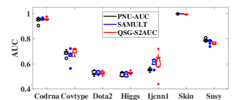
Figure 2: The boxplot of testing AUC results for PNU-AUC, SAMULT and our QSG-S2AUC.

Remark 1

According to Lemmas 1 and 2, the error caused by random features has the convergence rate of $O(1/t)$ with proper learning rate and $\theta\lambda\in(1,2)$.

Lemma 3 (Error due to random data)

Set $\eta_{t}=\dfrac{\theta}{t}$, $\theta>0$, such that $\theta\lambda\in(1,2)\cup\mathbb{Z}_{+}$, we have

$$\mathbb{E}_{x_{t}^{p},x_{t}^{n},x_{t}^{u},\omega_{t}}\left[\|h_{t+1}-f^{*}\|_{\mathcal{H}}^{2}\right]\leq\dfrac{Q_{1}^{2}}{t},$$ (19)

where $Q_{1}=\max\left\{\|f^{*}\|_{\mathcal{H}},\frac{Q_{0}+\sqrt{Q_{0}^{2}+(2\theta\lambda-1)(1+\theta\lambda)^{2}\theta^{2}\kappa M^{2}}}{2\theta\lambda-1}\right\}$, $Q_{0}=\sqrt{2}\kappa^{1/2}(\kappa+\phi)LM\theta^{2}$ and $L=\gamma(L_{1}+L_{2})+(1-\gamma)(L_{3}+L_{4}+L_{5}+L_{6})$.

According to Lemmas 1 and 3, we can obtain the convergence rate of QSG-S2AUC in Theorem 1.

Theorem 1 (Convergence in expectation)

Let $\chi$ denote the whole training set in semi-supervised learning problem. Set $\eta_{t}=\dfrac{\theta}{t}$, $\theta>0$, such that $\theta\lambda\in(1,2)\cup\mathbb{Z}_{+}$. $\forall x\in\chi$, we have

$$\mathbb{E}_{x_{t}^{p},x_{t}^{n},x_{t}^{u},\omega_{t}}\left[|f_{t+1}(x)-f^{*}(x)|^{2}\right]\leq\dfrac{2C^{2}+2\kappa Q^{2}_{1}}{t},$$

where $C^{2}=(\kappa+\phi)^{2}M^{2}\theta^{2}$.

Remark 2

Theorem 1 shows that for any given $x$, the evaluated value of $f_{t+1}$ at $x$ will converge to that of $f^{*}$ in terms of the Euclidean distance at the rate of $O(1/t)$. This rate is the same as that of standard DSG even though our problem is much more complicated and has four sources of randomness.

6 Experiments

In this section, we present the experimental results on several datasets to demonstrate the effectiveness and efficiency of QSG-S2AUC.

6.1 Experimental Setup

We compare the AUC results and running time of QSG-S2AUC with the state-of-the-art semi-supervised AUC maximization algorithms as summarized as follows.

1. PNU-AUC: Unbiased semi-supervised AUC optimization method proposed in  Sakai et al. (2018) based on positive and unlabeled learning.

2. SAMULT: The method proposed in  Xie and Li (2018) which does not require the class prior distribution to achieve the unbiased solution.

All the experiments were ran on a PC with 56 2.2GHz cores and 80GB RAM. We implemented QSG-S2AUC and SAMULT algorithms in MATLAB. We used the MATLAB code from https://github.com/t-sakai-kure/PNU as the implementation of PNU-AUC. For all algorithms, we use the square pairwise loss $l(u,v)=(1-u+v)^{2}$ and Gaussian kernel $k(x,x^{\prime})=\exp(-\sigma\|x-x^{\prime}\|^{2})$. The hyper-parameters ($\lambda$, $\sigma$ and $\gamma$) are chosen via 5-fold cross-validation. $\lambda$ and $\sigma$ were searched in the region $\{(\lambda,\sigma)|2^{-3}\leq\lambda\leq 2^{3},\;2^{-3}\leq\sigma\leq 2^{3}\}$. The trade-off parameter $\gamma$ in SAMULT and QSG-S2AUC was searched from $0$ to $1$ at intervals of $0.1$, and that in PNU-AUC was searched from $-1$ to $1$ at intervals of $0.1$. In addition, the class prior $\pi$ in PNU-AUC is set to the class proportion in the whole training set, which can be estimated by  du Plessis et al. (2015). All the results are the average of 10 trials.

6.2 Datasets

We carry out the experiments on eight large scale benchmark datasets collected from LIBSVM and UCI repositories. The size $n$ of the dataset and the feature dimensionality $d$ are summarized in Table 2. To conduct the experiments for semi-supervised learning, we randomly sample 200 labeled instances and treat the rest of the data as unlabeled. All the data features are normalized to $[0,1]$ in advance.

6.3 Results and Discussion

Figure 1 shows the training time of the three algorithms against different sizes of unlabeled samples on the eight benchmark datasets, where the sizes of labeled samples are fixed at 200. We can find that QSG-S2AUC is always faster than SAMULT and PNU-AUC. This is because the SAMULT and PNU-AUC need $O(n^{3})$ operations to compute the inverse matrixes with kernel. Differently, QSG-S2AUC uses RFF to approximate the kernel function, and each time it only needs $O(D)$ operations to calculate the random features with seed $i$. In addition, the low memory requirement of QSG-S2AUC allows it to do an efficient training for large scale datasets while PNU-AUC and SAMULT are out of memory. Figure 2 presents the testing AUC results of these algorithms on the eight benchmark datasets. The results show that QSG-S2AUC has the similar AUC results with other methods on the most datasets, and has the highest AUC on the datasets of Covtype and Ijcnn1. Based on these results, we conclude that QSG-S2AUC is superior to other state-of-the-art algorithms in terms of efficiency and scalability, while retaining the similar generalization performance.

7 Conclusion

In this paper, we propose a novel scalable semi-supervised AUC optimization algorithm, QSG-S2AUC. Considering that semi-supervised learning contains three data sources, DSG-S2AUC is designed to randomly sample one instance from each data source in each iteration. Then, their random features are generated and used to calculate a quadruply stochastic functional gradient for model update. Even though this optimization process contains multiple layers of stochastic sampling, theoretically, we prove that QSG-S2AUC has a convergence rate of $O(1/t)$. The experimental results on various datasets also demonstrate the superiority of the proposed QSG-S2AUC.

Appendix A Detailed Proof of Convergence Rate

In this section, we give detailed proof of Lemmas 1-3 and Theorem 1.

A.1 Proof of Lemma 1

Here we give the detailed proof of Lemma 1.

Proof 1

We denote $A_{i}(x)=A_{i}(x;x_{i}^{p},x_{i}^{n},x_{i}^{u},\omega_{i}):=a_{t}^{i}(\zeta_{i}(x)-\xi_{i}(x))$. According to the assumption in section 5, $A_{i}(X)$ have a bound:

$$|A_{i}(x)| \leq |a_{t}^{i}|\left(|\zeta_{i}(x)|+|\xi_{i}(x)|\right)$$

$$\leq |a_{t}^{i}|(\gamma(l^{\prime}_{1}k(x_{i}^{p},x)+l^{\prime}_{2}k(x_{i}^{n},x))$$

$$+(1-\gamma)(l^{\prime}_{3}k(x_{i}^{p},x)+l^{\prime}_{4}k(x_{i}^{u},x)$$

$$+l^{\prime}_{5}k(x_{i}^{u},x)+l^{\prime}_{6}k(x_{i}^{n},x))$$

$$+\gamma(l_{1}^{\prime}\phi_{\omega}(x^{p})\phi_{\omega}(x)+l_{2}^{\prime}\phi_{\omega}(x^{n})\phi_{\omega}(x)$$

$$+(1-\gamma)(l_{3}^{\prime}\phi_{\omega}(x^{p})\phi_{\omega}(x)+l_{4}^{\prime}\phi_{\omega}(x^{u})\phi_{\omega}(x)$$

$$+l_{5}^{\prime}\phi_{\omega}(x^{u})\phi_{\omega}(x)+l_{6}^{\prime}\phi_{\omega}(x^{n})\phi_{\omega}(x))))$$

$$\leq |a_{t}^{i}|((\gamma(M_{1}+M_{2})$$

$$+(1-\gamma)(M_{3}+M_{4}+M_{5}+M_{6}))\kappa$$

$$+(\gamma(M_{1}+M_{2})$$

$$+(1-\gamma)(M_{3}+M_{4}+M_{5}+M_{6}))\phi)$$

$$= M(\kappa+\phi)|a_{t}^{i}|$$

Then we obtain the lemma 1. This completes the proof.

A.2 Proof of lemma 2

Here we give detailed proof of Lemma 2.

Proof 2

Obviously, $|a_{t}^{i}|\leq\dfrac{\theta}{t}$. Then we have

$$|a_{t}^{i}| =|a_{t}^{i+1}\dfrac{\eta_{i}}{\eta_{i+1}}(1-\lambda\eta_{i+1})|$$

$$=\dfrac{i+1}{i}|1-\dfrac{\lambda\theta}{i+1}|\cdot|a_{t}^{i+1}|$$

$$=|\dfrac{i+1-\lambda\theta}{i}|\cdot|a_{t}^{i+1}|$$

When $\lambda\theta\in(1,2),\forall i\geq 1$, we have $i-1<i+1-\lambda\theta<i$, so $|a_{t}^{i}|<|a_{t}^{i+1}|\leq\dfrac{\theta}{t}$ and $\sum_{i=1}^{t}\leq\dfrac{\theta^{2}}{t}$. When $\lambda\theta\in\mathbb{Z}_{+}$, if $i>\lambda\theta-1$, then $|a_{t}^{i}|<|a_{t}^{i+1}|\leq\dfrac{\theta}{t}$. If $i\leq\lambda\theta-1$, then $|a_{t}^{i}|=0$. So we get $\sum_{i=1}^{t}|a_{t}^{i}|^{2}\leq\dfrac{\theta^{2}}{t}$. Therefore, we obtain the lemma 2. This completes the proof.

A.3 Proof of Lemma 3

For convenience, we denote that $l_{1}^{\prime}(f(x_{t}^{p}),f(x_{t}^{n}))$, $l_{2}^{\prime}(f(x_{t}^{p}),f(x_{t}^{n}))$, $l_{3}^{\prime}(f(x_{t}^{p}),f(x_{t}^{u}))$, $l_{4}^{\prime}(f(x_{t}^{p}),f(x_{t}^{u}))$, $l_{5}^{\prime}(f(x_{t}^{u}),f(x_{t}^{n}))$ and $l_{6}^{\prime}(f(x_{t}^{u}),f(x_{t}^{n}))$ as $l_{1}^{\prime}(f_{t})$, $l_{2}^{\prime}(f_{t})$, $l_{3}^{\prime}(f_{t})$, $l_{4}^{\prime}(f_{t})$, $l_{5}^{\prime}(f_{t})$ and $l_{6}^{\prime}(f_{t})$, respectively. In addition, we define the following three different gradient terms,

$$g_{t} = \xi_{t}+\lambda h_{t}$$

$$= \gamma(l_{1}^{\prime}(f_{t})k(x_{t}^{p},\cdot)+l_{2}^{\prime}(f_{t})k(x_{t}^{n},\cdot))$$

$$+(1-\gamma)(l_{3}^{\prime}(f_{t})k(x_{t}^{p},\cdot)+l_{4}^{\prime}(f_{t})k(x_{t}^{u},\cdot)$$

$$+l_{5}^{\prime}(f_{t})k(x_{t}^{u},\cdot)+l_{6}^{\prime}(f_{t})k(x_{t}^{n},\cdot))+\lambda h_{t}$$

$$\hat{g_{t}} = \hat{\xi_{t}}+\lambda h_{t}$$

$$= \gamma(l_{1}^{\prime}(h_{t})k(x_{t}^{p},\cdot)+l_{2}^{\prime}(h_{t})k(x_{t}^{n},\cdot))$$

$$+(1-\gamma)(l_{3}^{\prime}(h_{t})k(x_{t}^{p},\cdot)+l_{4}^{\prime}(h_{t})k(x_{t}^{u},\cdot)$$

$$+l_{5}^{\prime}(h_{t})k(x_{t}^{u},\cdot)+l_{6}^{\prime}(h_{t})k(x_{t}^{n},\cdot))+\lambda h_{t}$$

$$\bar{g_{t}} = \mathbb{E}_{x_{t}^{p},x_{t}^{n},x_{t}^{u}}[\hat{g_{t}}]$$

$$= \mathbb{E}_{x_{t}^{p},x_{t}^{n}x_{t}^{u}}[\gamma(l_{1}^{\prime}(h_{t})k(x_{t}^{p},\cdot)+l_{2}^{\prime}(h_{t})k(x_{t}^{n},\cdot))$$

$$+(1-\gamma)(l_{3}^{\prime}(h_{t})k(x_{t}^{p},\cdot)+l_{4}^{\prime}(h_{t})k(x_{t}^{u},\cdot)$$

$$+l_{5}^{\prime}(h_{t})k(x_{t}^{u},\cdot)+l_{6}^{\prime}(h_{t})k(x_{t}^{n},\cdot))]+\lambda h_{t}$$

Note that from our previous definition, we have $h_{t+1}=h_{t}-\eta_{t}g_{t},\forall t\geq 1$.

Denote $A_{t}=\parallel h_{t}-f^{*}\parallel_{\mathcal{H}}^{2}$. Then we have

$$A_{t+1} = \parallel h_{t}-f^{*}-\eta_{t}g_{t}\parallel_{\mathcal{H}}^{2}$$

$$= A_{t}+\eta_{t}^{2}\parallel g_{t}\parallel_{\mathcal{H}}^{2}-2\eta_{t}\langle h_{t}-f^{*},g_{t}\rangle_{\mathcal{H}}$$

$$= A_{t}+\eta_{t}^{2}\parallel g_{t}\parallel_{\mathcal{H}}^{2}-2\eta_{t}\langle h_{t}-f^{*},\bar{g_{t}}\rangle_{\mathcal{H}}$$

$$+2\eta_{t}\langle h_{t}-f^{*},\bar{g_{t}}-\hat{g_{t}}\rangle_{\mathcal{H}}+2\eta_{t}\langle h_{t}-f^{*},\hat{g_{t}}-g_{t}\rangle_{\mathcal{H}}$$

Because of the strongly convexity of loss function and optimality condition, we have

$$\langle h_{t}-f^{*},\bar{g_{t}}\rangle_{\mathcal{H}}\geq\lambda\parallel h_{t}-f^{*}\parallel_{\mathcal{H}}^{2}$$

Hence, we have

$$A_{t+1} \leq(1-2\eta_{t}\lambda)A_{t}+\eta_{t}^{2}\parallel g_{t}\parallel_{\mathcal{H}}^{2}+2\eta_{t}\langle h_{t}-f^{*},\bar{g_{t}}-\hat{g_{t}}\rangle_{\mathcal{H}}$$

$$\quad+2\eta_{t}\langle h_{t}-f^{*},\hat{g_{t}}-g_{t}\rangle_{\mathcal{H}},\forall t\geq 1$$ (20)

Let us denote $\mathcal{M}_{t}=\parallel g_{t}\parallel_{\mathcal{H}}^{2}$, $\mathcal{N}_{t}=\langle h_{t}-f^{*},\bar{g_{t}}-\hat{g_{t}}\rangle_{\mathcal{H}}$, $\mathcal{R}_{t}=\langle h_{t}-f^{*},\hat{g_{t}}-g_{t}\rangle_{\mathcal{H}}$. Firstly, we show that $\mathcal{M}_{t}$, $\mathcal{N}_{t}$, $\mathcal{R}_{t}$ are bounded. Specifically, for $t\geq 1$, we have

$$\mathcal{M}_{t}\leq\kappa M^{2}(1+\lambda c_{t})$$ (21)

where $c_{t}:=\sqrt{\sum_{i,j=1}^{t-1}|a_{t-1}^{i}||a_{t-1}^{j}|}$

$$\mathbb{E}_{x_{t}^{p},x_{t}^{n},x_{t}^{u},\omega_{t}}[\mathcal{N}_{t}]=0$$ (22)

$$\mathbb{E}_{x_{t}^{p},x_{t}^{n}x_{t}^{u},\omega_{t}}[\mathcal{R}_{t}]\leq\kappa^{1/2}LB_{1,t}\sqrt{\mathbb{E}_{x_{t-1}^{p},x_{t-1}^{n},x_{t-1}^{u},\omega_{t-1}}[A_{t}]}$$ (23)

where $M:=\gamma(M_{1}+M_{2})+(1-\gamma)(M_{3}+M_{4}+M_{5}+M_{6})$, $L:=\gamma(L_{1}+L_{2})+(1-\gamma)(L_{3}+L_{4}+L_{5}+L_{6})$ and $A_{t}=\parallel h_{t}-f^{*}\parallel_{\mathcal{H}}^{2}$.

Proof 3

The proof of Eq. (21):

$$\mathcal{M}_{t}=\parallel g_{t}\parallel_{\mathcal{H}}^{2}=\parallel\xi_{t}+\lambda h_{t}\parallel_{\mathcal{H}}^{2}\leq\left(\parallel\xi\parallel_{\mathcal{H}}+\lambda\parallel h_{t}\parallel_{\mathcal{H}}\right)^{2}$$

and

$$\parallel\xi_{t}\parallel_{\mathcal{H}} = \parallel\gamma(l_{1}^{\prime}(f_{t})k(x_{t}^{p},\cdot)+l_{2}^{\prime}(f_{t})k(x_{t}^{n},\cdot))$$

$$+(1-\gamma)(l_{3}^{\prime}(f_{t})k(x_{t}^{p},\cdot)+l_{4}^{\prime}(f_{t})k(x_{t}^{u},\cdot)$$

$$+l_{5}^{\prime}(f_{t})k(x_{t}^{u},\cdot)+l_{6}^{\prime}(f_{t})k(x_{t}^{n},\cdot))\parallel_{\mathcal{H}}$$

$$\leq \kappa^{1/2}(\gamma(M_{1}+M_{2})$$

$$+(1-\gamma)(M_{3}+M_{4}+M_{5}+M_{6}))$$

$$= \kappa^{1/2}M$$

Then we have:

$$\|h_{t}\|_{\mathcal{H}}^{2} = \sum_{i=1}^{t-1}\sum_{j=1}^{t-1}a_{t-1}^{i}a_{t-1}^{j}[\gamma(l_{1}^{\prime}k(x_{i}^{p},\cdot)+l_{2}^{\prime}k(x_{i}^{n},\cdot))$$

$$+(1-\gamma)(l_{3}^{\prime}k(x_{i}^{p},\cdot)+l_{4}^{\prime}k(x_{i}^{u},\cdot)$$

$$+l_{5}^{\prime}k(x_{i}^{u},\cdot)+l_{6}^{\prime}k(x_{i}^{n},\cdot))]$$

$$\cdot[\gamma(l_{1}^{\prime}k(x_{j}^{p},\cdot)+l_{2}^{\prime}k(x_{j}^{n},\cdot))$$

$$+(1-\gamma)(l_{3}^{\prime}k(x_{j}^{p},\cdot)+l_{4}^{\prime}k(x_{j}^{u},\cdot)$$

$$+l_{5}^{\prime}k(x_{j}^{u},\cdot)+l_{6}^{\prime}k(x_{j}^{n},\cdot))]$$

$$\leq \kappa\sum_{i=1}^{t-1}\sum_{j=1}^{t-1}a_{t-1}^{i}a_{t-1}^{j}[\gamma^{2}(M_{1}+M_{2})^{2}$$

$$+2\gamma(1-\gamma)(M_{1}+M_{2})(M_{3}+M_{4}+M_{5}+M_{6})$$

$$+(1-\gamma)^{2}(M_{3}+M_{4}+M_{5}+M_{6})^{2}]$$

$$= \kappa\sum_{i=1}^{t-1}\sum_{j=1}^{t-1}a_{t-1}^{i}a_{t-1}^{j}[\gamma(M_{1}+M_{2})$$

$$+(1-\gamma)(M_{3}+M_{4}+M_{5}+M_{6})]^{2}$$

$$= \kappa M^{2}\sum_{i=1}^{t-1}\sum_{j=1}^{t-1}a_{t-1}^{i}a_{t-1}^{j}$$

Then we obtain Eq. (21).

Proof 4

The proof of Eq. (22)

$$\mathbb{E}_{x_{t}^{p},x_{t}^{n},x_{t}^{u},\omega_{t}}[\mathcal{N}_{t}]$$

$$= \mathbb{E}_{x_{t-1}^{p},x_{t-1}^{n},x_{t-1}^{u},\omega_{t}}$$

$$\left[\mathbb{E}_{x_{t}^{p},x_{t}^{n},x_{t}^{u}}[\langle h_{t}-f^{*},\bar{g_{t}}-\hat{g_{t}}\rangle_{\mathcal{H}}|x_{t-1}^{p},x_{t-1}^{u},\omega_{t}]\right]$$

$$= \mathbb{E}_{x_{t-1}^{p},x_{t-1}^{n},x_{t-1}^{u},\omega_{t}}\left[\langle h_{t}-f^{*},\mathbb{E}_{x_{t-1}^{p},x_{t-1}^{n},x_{t-1}^{u}}[\bar{g_{t}}-\hat{g_{t}}]\rangle_{\mathcal{H}}\right]$$

$$= 0$$

Proof 5

The proof of Eq. (23)

$$\mathbb{E}_{x_{t}^{p},x_{t}^{n},x_{t}^{u},\omega_{t}}[\mathcal{R}_{t}]$$

$$= \mathbb{E}_{x_{t}^{p},x_{t}^{n},x_{t}^{u},\omega_{t}}[\langle h_{t}-f^{*},\hat{g_{t}}-g_{t}\rangle_{\mathcal{H}}]$$

$$= \mathbb{E}_{x_{t}^{p},x_{t}^{n},x_{t}^{u},\omega_{t}}[\langle h_{t}-f^{*},\gamma[(l^{\prime}_{1}(f_{t})-l^{\prime}_{1}(h_{t}))k(x_{t}^{p},\cdot)$$

$$+(l^{\prime}_{2}(f_{t})-l^{\prime}_{2}(h_{t}))k(x_{t}^{n},\cdot)]$$

$$+(1-\gamma)[(l^{\prime}_{3}(f_{t})-l^{\prime}_{3}(h_{t}))k(x_{t}^{p},\cdot)$$

$$+(l^{\prime}_{4}(f_{t})-l^{\prime}_{4}(h_{t}))k(x_{t}^{u},\cdot)$$

$$+(l^{\prime}_{5}(f_{t})-l^{\prime}_{5}(h_{t}))k(x_{t}^{u},\cdot)$$

$$+(l^{\prime}_{6}(f_{t})-l^{\prime}_{6}(h_{t}))k(x_{t}^{n},\cdot)]\rangle_{\mathcal{H}}]$$

$$\leq \mathbb{E}_{x_{t}^{p},x_{t}^{p},x_{t}^{u},\omega_{t}}[\parallel h_{t}-f^{*}\parallel_{\mathcal{H}}$$

$$\cdot\gamma[|l^{\prime}_{1}(f_{t})-l^{\prime}_{1}(h_{t})|\cdot\parallel k(x_{t}^{p},\cdot)\parallel_{\mathcal{H}}$$

$$+|l^{\prime}_{2}(f_{t})-l^{\prime}_{2}(h_{t})|\parallel k(x_{t}^{n},\cdot)\parallel_{\mathcal{H}}]$$

$$+(1-\gamma)[|l^{\prime}_{3}(f_{t})-l^{\prime}_{3}(h_{t})|\parallel k(x_{t}^{p},\cdot)\parallel_{\mathcal{H}}$$

$$+|l^{\prime}_{4}(f_{t})-l^{\prime}_{4}(h_{t})|\parallel k(x_{t}^{u},\cdot)\parallel_{\mathcal{H}}$$

$$+|l^{\prime}_{5}(f_{t})-l^{\prime}_{5}(h_{t})|\parallel k(x_{t}^{u},\cdot)\parallel_{\mathcal{H}}$$

$$+|l^{\prime}_{6}(f_{t})-l^{\prime}_{6}(h_{t})|\parallel k(x_{t}^{n},\cdot)\parallel_{\mathcal{H}}]]$$

$$\leq \kappa^{1/2}\mathbb{E}_{x_{t}^{p},x_{t}^{u},x_{t}^{u},\omega_{t}}[\parallel h_{t}-f^{*}\parallel_{\mathcal{H}}$$

$$\cdot[\gamma(|l^{\prime}_{1}(f_{t})-l^{\prime}_{1}(h_{t})|$$

$$+|l^{\prime}_{2}(f_{t})-l^{\prime}_{2}(h_{t})|)$$

$$+(1-\gamma)(|l^{\prime}_{3}(f_{t})-l^{\prime}_{3}(h_{t})|$$

$$+|l^{\prime}_{4}(f_{t})-l^{\prime}_{4}(h_{t})|$$

$$+|l^{\prime}_{5}(f_{t})-l^{\prime}_{5}(h_{t})|$$

$$+|l^{\prime}_{6}(f_{t})-l^{\prime}_{6}(h_{t})|)]]$$

$$\leq \kappa^{1/2}\mathbb{E}_{x_{t}^{p},x_{t}^{n},x_{t}^{u},\omega_{t}}[\|h_{t}-f^{*}\|_{\mathcal{H}}$$

$$\cdot[\gamma(L_{1}|f_{t}(x_{t}^{p})-h_{t}(x_{t}^{p})|$$

$$+L_{2}|f_{t}(x_{t}^{n})-h_{t}(x_{t}^{n})|)$$

$$+(1-\gamma)(L_{3}|f_{t}(x_{t}^{p})-h_{t}(x_{t}^{p})|$$

$$+L_{4}|f_{t}(x_{t}^{u})-h_{t}(x_{t}^{u})|$$

$$+L_{5}|f_{t}(x_{t}^{u})-h_{t}(x_{t}^{u})|$$

$$+L_{6}|f_{t}(x_{t}^{n})-h_{t}(x_{t}^{n})|)]]$$

$$\leq \kappa^{1/2}\sqrt{\mathbb{E}_{x_{t}^{p},x_{t}^{n},x_{t}^{u},\omega_{t}}[A_{t}]}$$

$$\cdot\sqrt{[\gamma(L_{1}+L_{2})+(1-\gamma)(L_{3}+L_{4}+L_{5}+L_{6})]^{2}B_{1,t}^{2}}$$

$$\leq \kappa^{1/2}LB_{1,t}\sqrt{\mathbb{E}_{x_{t-1}^{p},x_{t-1}^{n},x_{t-1}^{u},\omega_{t-1}}[A_{t}]}$$

The first and third inequalities are due to Cauchy-Schwarz Inequality and the second inequality is due to the Assumption 3. And the last step is due to the Lemma 1 and the definition of $A_{t}$.

After proving the Eq. (21)-(23) separately, let us denote $e_{t}=\mathbb{E}_{x_{t}^{p},x_{t}^{u},\omega_{t}}[A_{t}]$, given the above bounds, we arrive the following recursion,

$$e_{t+1}\leq(1-2\eta_{t}\lambda)e_{t}+\kappa M^{2}\eta_{t}^{2}(1+\lambda c_{t})^{2}+2\kappa^{1/2}L\eta_{t}B_{1,t}\sqrt{e_{t}}$$

When $\eta_{t}=\dfrac{\theta}{t}$ with $\theta$ such that $\theta\lambda\in(1,2)\cup\mathbb{Z}_{+}$, from Lemma 2, we have $|a_{t}^{i}|\leq\dfrac{\theta}{t}$, $\forall 1\leq i\leq t$. Consequently, $c_{t}\leq\theta$ and $B_{1,t}^{2}\leq M^{2}(\kappa+\phi)^{2}\dfrac{\theta^{2}}{t-1}$. Applying these bounds to the above recursion, we have $e_{t+1}\leq(1-\dfrac{2\theta\lambda}{t})e_{t}+\kappa^{2}\dfrac{\theta^{2}}{t^{2}}(1+\lambda\theta)^{2}+2\kappa^{1/2}\dfrac{\theta}{t}L\eta_{t}\sqrt{M^{2}(\kappa+\phi)^{2}\dfrac{\theta^{2}}{t-1}}\sqrt{e_{t}}$ and then it can be rewritten as:

$$e_{t+1}\leq(1-\dfrac{2\theta\lambda}{t})e_{t}+\dfrac{\beta_{1}}{t}\sqrt{\dfrac{e_{t}}{t}}+\dfrac{\beta_{2}}{t^{2}}$$

where $\beta_{1}=2\sqrt{2}\kappa^{1/2}LM(\kappa+\phi)\theta^{2}$ ($\sqrt{\dfrac{t}{t-q}}\leq\sqrt{2}$) and $\beta_{2}=\kappa M^{2}\theta^{2}(1+\lambda\theta)^{2}$. Reusing Lemma 14 in [Dai et al., 2014] with $\eta=2\theta\lambda>1$ leads to

$$e_{t+1}\leq\dfrac{Q_{1}^{2}}{t}$$

where

$$Q_{1}=\max\left\{\parallel f^{*}\parallel_{\mathcal{H}},\dfrac{Q_{0}+\sqrt{Q_{0}^{2}+(2\theta\lambda-1)(1+\theta\lambda)^{2}\theta^{2}\kappa M^{2}}}{2\theta\lambda-1}\right\}$$

and $Q_{0}=2\sqrt{2}\kappa^{1/2}(\kappa+\phi)LM\theta^{2}$.

A.4 Proof of Theorem 1

Finally, we give the proof of Theorem 1.

Proof 6

Substitute Lemma 1 and 3 into Eq. (17), we have that

$$\mathbb{E}_{x_{t}^{p},x_{t}^{u},\omega_{t}}[|f_{t}(x)-f^{*}(x)|^{2}] \leq 2\mathbb{E}_{x_{t}^{p},x_{t}^{u},\omega_{t}}[|f_{t}(x)-h_{t+1}(x)|^{2}]$$

$$+2\kappa\mathbb{E}_{x_{t}^{p},x_{t}^{u},\omega_{t}}[\parallel h_{t}-f^{*}\parallel_{\mathcal{H}}]$$

$$\leq 2B_{1,t+1}^{2}+2\kappa\dfrac{Q_{1}^{2}}{t}$$

$$\leq \dfrac{2C^{2}+2\kappa Q_{1}^{2}}{t}$$

where the last inequality is due to Lemma 2. In this way, we obtain the final result on convergence in expectation. This completes the proof.

References

• Amini et al. [2008] Massih-Reza Amini, Tuong-Vinh Truong, and Cyril Goutte. A boosting algorithm for learning bipartite ranking functions with partially labeled data. 2008.
• Dai et al. [2014] Bo Dai, Bo Xie, Niao He, Yingyu Liang, Anant Raj, Maria-Florina F Balcan, and Le Song. Scalable kernel methods via doubly stochastic gradients. In Advances in Neural Information Processing Systems, pages 3041–3049, 2014.
• Ding et al. [2017] Yi Ding, Chenghao Liu, Peilin Zhao, and Steven CH Hoi. Large scale kernel methods for online auc maximization. In 2017 IEEE International Conference on Data Mining (ICDM), pages 91–100. IEEE, 2017.
• Drineas and Mahoney [2005] Petros Drineas and Michael W Mahoney. On the nyström method for approximating a gram matrix for improved kernel-based learning. journal of machine learning research, 6(Dec):2153–2175, 2005.
• du Plessis et al. [2015] Marthinus Christoffel du Plessis, Gang Niu, and Masashi Sugiyama. Class-prior estimation for learning from positive and unlabeled data. In ACML, pages 221–236, 2015.
• Fine and Scheinberg [2001] Shai Fine and Katya Scheinberg. Efficient svm training using low-rank kernel representations. Journal of Machine Learning Research, 2(Dec):243–264, 2001.
• Fujino and Ueda [2016] Akinori Fujino and Naonori Ueda. A semi-supervised auc optimization method with generative models. In Data Mining (ICDM), 2016 IEEE 16th International Conference on, pages 883–888. IEEE, 2016.
• Gao and Zhou [2015] Wei Gao and Zhi-Hua Zhou. On the consistency of auc pairwise optimization. In IJCAI, pages 939–945, 2015.
• Gao et al. [2013] Wei Gao, Rong Jin, Shenghuo Zhu, and Zhi-Hua Zhou. One-pass auc optimization. In International Conference on Machine Learning, pages 906–914, 2013.
• Geng et al. [2019] Xiang Geng, Bin Gu, Xiang Li, Wanli Shi, Guansheng Zheng, and Heng Huang. Scalable semi-supervised svm via triply stochastic gradients. In 28th International Joint Conference on Artificial Intelligence, 2019.
• Gu and Huo [2018] Bin Gu and Zhouyuan Huo. Asynchronous doubly stochastic group regularized learning. In International Conference on Artificial Intelligence and Statistics (AISTATS 2018), 2018.
• Gu et al. [2014] Bin Gu, Victor S Sheng, Keng Yeow Tay, Walter Romano, and Shuo Li. Incremental support vector learning for ordinal regression. IEEE Transactions on Neural networks and learning systems, 26(7):1403–1416, 2014.
• Gu et al. [2016] Bin Gu, Zhouyuan Huo, and Heng Huang. Asynchronous stochastic block coordinate descent with variance reduction. arXiv preprint arXiv:1610.09447, 2016.
• Gu et al. [2018a] Bin Gu, Yingying Shan, Xiang Geng, and Guansheng Zheng. Accelerated asynchronous greedy coordinate descent algorithm for svms. In IJCAI, pages 2170–2176, 2018.
• Gu et al. [2018b] Bin Gu, Miao Xin, Zhouyuan Huo, and Heng Huang. Asynchronous doubly stochastic sparse kernel learning. In Thirty-Second AAAI Conference on Artificial Intelligence, 2018.
• Gu et al. [2018c] Bin Gu, Xiao-Tong Yuan, Songcan Chen, and Heng Huang. New incremental learning algorithm for semi-supervised support vector machine. In Proceedings of the 24th ACM SIGKDD International Conference on Knowledge Discovery & Data Mining, pages 1475–1484. ACM, 2018.
• Hanley and McNeil [1982] James A Hanley and Barbara J McNeil. The meaning and use of the area under a receiver operating characteristic (roc) curve. Radiology, 143(1):29–36, 1982.
• Huang et al. [2019] Feihu Huang, Bin Gu, Zhouyuan Huo, Songcan Chen, and Heng Huang. Faster gradient-free proximal stochastic methods for nonconvex nonsmooth optimization. arXiv preprint arXiv:1902.06158, 2019.
• Li et al. [2017] Xiang Li, Bin Gu, Shuang Ao, Huaimin Wang, and Charles X Ling. Triply stochastic gradients on multiple kernel learning. UAI, 2017.
• Liang [2005] Percy Liang. Semi-supervised learning for natural language. PhD thesis, Massachusetts Institute of Technology, 2005.
• Liu et al. [2018] Mingrui Liu, Xiaoxuan Zhang, Zaiyi Chen, Xiaoyu Wang, and Tianbao Yang. Fast stochastic auc maximization with o (1/n)-convergence rate. In International Conference on Machine Learning, pages 3195–3203, 2018.
• Rahimi and Recht [2008] Ali Rahimi and Benjamin Recht. Random features for large-scale kernel machines. In Advances in neural information processing systems, pages 1177–1184, 2008.
• Rudin [2017] Walter Rudin. Fourier analysis on groups. Courier Dover Publications, 2017.
• Sakai et al. [2017] Tomoya Sakai, Marthinus Christoffel du Plessis, Gang Niu, and Masashi Sugiyama. Semi-supervised classification based on classification from positive and unlabeled data. In Proceedings of the 34th International Conference on Machine Learning-Volume 70, pages 2998–3006. JMLR. org, 2017.
• Sakai et al. [2018] Tomoya Sakai, Gang Niu, and Masashi Sugiyama. Semi-supervised auc optimization based on positive-unlabeled learning. Machine Learning, 107(4):767–794, 2018.
• Sholokhov et al. [2018] Alexey Sholokhov, Md Sahidullah, and Tomi Kinnunen. Semi-supervised speech activity detection with an application to automatic speaker verification. Computer Speech & Language, 47:132–156, 2018.
• Smola and Schölkopf [2000] Alex J Smola and Bernhard Schölkopf. Sparse greedy matrix approximation for machine learning. 2000.
• Wang et al. [2010] Jun Wang, Sanjiv Kumar, and Shih-Fu Chang. Semi-supervised hashing for scalable image retrieval. 2010.
• Xie and Li [2018] Zheng Xie and Ming Li. Semi-supervised auc optimization without guessing labels of unlabeled data. 2018.
• Ying et al. [2016] Yiming Ying, Longyin Wen, and Siwei Lyu. Stochastic online auc maximization. In Advances in neural information processing systems, pages 451–459, 2016.
• Yu et al. [2019] Shuyang Yu, Bin Gu, Kunpeng Ning, Haiyan Chen, Jian Pei, and Heng Huang. Tackle balancing constraint for incremental semi-supervised support vector learning. In Proceedings of the 25th ACM SIGKDD International Conference on Knowledge Discovery & Data Mining, 2019.