Empirical strategy-proofness

Abstract

Empirical tests of direct revelation games of strategy-proof social choice functions show behavior in these games can approximate suboptimal mutual best responses. We determine that this worst case scenario for the operation of these mechanisms is only likely to be observed when the social choice function violates a non-bossiness condition and information is not interior. Our analysis is based on an empirical approach to the refinement of Nash equilibrium that we introduce, and the characterization of direct robust full implementation based on this solution concept. Experimental and empirical evidence on these games supports our findings.

JEL classification: C72, D47, D91.

Keywords: behavioral mechanism design; empirical equilibrium; robust mechanism design; strategy-proofness.

1 Introduction

Strategy proofness, a coveted property in market design, requires that truthful reports be dominant strategies in the simultaneous direct revelation game associated with a social choice function (scf). Despite the theoretical appeal of this property, experimental and empirical evidence suggests that when an scf satisfying this property is operated, agents may persistently exhibit weakly dominated behavior. This includes experiments with diverse mechanisms (Coppinger et al., 1980; Kagel et al., 1987; Kagel and Levin, 1993; Harstad, 2000; Attiyeh et al., 2000; Chen and Sönmez, 2006; Cason et al., 2006; Healy, 2006; Andreoni et al., 2007; Li, 2017), survey evidence from national level matching platforms (Rees-Jones, 2017; Hassidim et al., 2020), and empirical evidence from school choice mechanisms (Artemov et al., 2020; Chen and Pereyra, 2019; Shorrer and Sóvágó, 2019). More strikingly, several studies have documented approximate suboptimal equilibria of these games (e.g., Cason et al. (2006); Healy (2006); Andreoni et al. (2007); see also Sec. 6 for a detailed analysis). That is, persistent weakly dominated behavior that approaches mutual best responses and produces with positive probability outcomes that are different from those intended by the social choice function. The purpose of this paper is to understand this phenomenon. That is, our objective is to unveil the conditions under which this worst case scenario for the operation of a strategy-proof social choice function can happen.

Our study contributes to the growing literature that, motivated by empirical evidence, studies which strategy-proof scfs admit implementation by means of mechanisms that have additional incentives properties. This literature has identified the conditions in which strategy-proof games have no sub-optimal equilibria (Saijo et al., 2007). It has also identified scfs that admit implementation by an extensive-form dominant strategy mechanism in which an agent’s choice of a dominant strategy is simpler than in the scf’s simultaneous direct revelation mechanism (Li, 2017; Pycia and Troyan, 2019). In many problems of interest these requirements lead to impossibilities (see Sec. 2 for details). Moreover, the empirical evidence against strategy-proof scfs is not universal for all scfs that violate these conditions. Thus, our study offers a fundamental categorization of strategy-proof scfs in the environments for which the further requirements of Saijo et al. (2007), Li (2017), and Pycia and Troyan (2019) cannot be met.

To understand why some suboptimal equilibria of strategy-proof games are empirically relevant, it is natural to analyze them based on an equilibrium refinement. These theories aim to select the Nash equilibria that are plausible in a game. Unfortunately, the most prominent refinements in the literature are silent about the nature of this phenomenon. They either implicitly or explicitly assume admissibility, i.e., that weakly dominated behavior is not plausible (from the seminal tremble-based refinements of Selten (1975) and Myerson (1978), to their most recent forms in Milgrom and Mollner (2017, 2018) and Fudenberg and He (2018); see also Kohlberg and Mertens (1986) and van Damme (1991) for a survey).

We propose an alternative path to refine Nash equilibria. It allows us to understand the incentives for truthful revelation across different strategy-proof mechanisms and to come to terms with the existing experimental and empirical evidence. Our refinement is based on an inverse approach to that taken by the existing tremble-based equilibrium refinements literature. At a high level, one can describe these refinements as follows. Based on a particular game in which a Nash equilibrium is intuitively implausible, the researchers identify a property that is not satisfied by this equilibrium but is always satisfied by some equilibrium in every possible game. Our proposal is to work in the opposite order. That is, we begin our quest by identifying a property of behavior that has empirical support and work our ways backward to identify the equilibria that can possibly be observed, at least approximately, if behavior will satisfy this property.

More formally, we articulate an empirical approach to refine Nash equilibria. That is, we consider a researcher who samples behavior in normal-form games and constructs a theory that explains it. The researcher then determines the plausibility of Nash equilibria based on the empirical content of the theory by requiring that Nash equilibria be in its closure. More precisely, if a Nash equilibrium cannot be approximated to an arbitrary degree by the empirical content of the researcher’s theory, it is identified as implausible or unlikely to be observed. One can give this approach a static or dynamic interpretation. First, it simply articulates the logical implication of the hypothesis that the researcher’s theory is well specified, for this hypothesis is refuted by the observation of a Nash equilibrium that is flagged as implausible. Alternatively, suppose that the researcher hypothesizes that behavior will eventually converge to a Nash equilibrium through an unmodeled evolutionary process that produces a path of behavior that is consistent with her theory. Then, the researcher can also conclude that the only Nash equilibria that are relevant are those that are not flagged as implausible.

To make this empirical approach concrete we identify a non-parametric theory for which there is empirical support. We consider a hypothetical environment in which a researcher observes payoffs, controls the information available to each agent, and samples behavior. This framework encompasses the experimental environments with monetary payoffs and the observable game matrix framework used for the foundation of Nash equilibrium by Harsanyi (1973). We observe that a common factor in the noisy best response models that have been proposed to account for observed behavior in these environments—either sampled or hypothetical as in Harsanyi (1973), require consistency with an a priori restriction for which there is empirical support, weak payoff monotonicity. This property of the full profile of empirical distributions of play in a game requires that for each agent, differences in behavior reveal differences in expected utility. That is, between two alternative actions for an agent, say $a$ and $b$, if the agent plays $a$ with higher frequency than $b$, it is because given what the other agents are doing, $a$ has higher expected utility than $b$ (see Sec. 3 for an intuitive example).

Empirical equilibrium is the refinement so defined based on weak payoff monotonicity, i.e., the one that selects each Nash equilibrium for which there is a sequence of weakly payoff monotone behavior that converges to it.

Empirical equilibria exist for each finite game and may admit weakly dominated behavior. Indeed, the limits of logistic QRE (as the noisy best responses converge to best responses) are empirical equilibria (McKelvey and Palfrey, 1995). It is known that for each finite game these limits exist and that they may admit weakly dominated behavior (McKelvey and Palfrey, 1995). Furthermore, empirical equilibrium is independent from the refinements previously defined in the literature. Determining this has a technical nature, which we have pursued in a companion paper (Velez and Brown, 2019b) (Sec. 2 summarizes these findings). Since our interest in this paper is the analysis of strategy-proof mechanisms, we concentrate on the application of the empirical equilibrium refinement to these games. It is worth noting that the games we analyze give us the chance to show the full power of this refinement to rule out implausible behavior without ruling out behavior that is prevalent in experiments.

We submit that we can considerably advance our understanding of the direct revelation game of a strategy-proof scf by calculating its empirical equilibria. On the one hand, suppose that we find that for a certain game each empirical equilibrium is truthful equivalent. Then, we learn that as long as empirical distributions of play are weakly payoff monotone, behavior will never approximate a sub-optimal Nash equilibrium. On the other hand, if we find that some empirical equilibria are not truthful equivalent, this alerts us about the possibility that we may plausibly observe persistent behavior that generates sub-optimal outcomes and approximates mutual best responses.

We present two main results. The first is that non-bosiness in welfare-outcome—i.e., the requirement on an scf that no agent be able to change the outcome without changing her own welfare—is necessary and sufficient to guarantee that for each common prior type space, each empirical equilibrium of the direct revelation game of a strategy-proof scf in a private values environment, produces, with certainty, the truthful outcome (Theorem 1). The second is that the requirement that a strategy-proof scf have essentially unique dominant strategies, characterizes this form of robust implementation for type spaces with full support (Theorem 2). The sharp predictions of our theorems are consistent with experimental and empirical evidence on strategy-proof mechanisms (Sec. 6). Indeed, they are in line with some of the most puzzling evidence on the second-price auction, a strategy-proof mechanism that violates non-bosiness but whose dominant strategies are unique. Deviations from truthful behavior are persistently observed when this mechanism is operated, but mainly for information structures for which agents’ types are common information (Andreoni et al., 2007).

The remainder of the paper is organized as follows. Section 2 places our contribution in the context of the literature. Section 3 presents the intuition of our results illustrated for the Top Trading Cycles (TTC) mechanism and the second-price auction, two cornerstones of the market design literature. Section 4 introduces the model. Section 5 presents our main results. Section 6 contrasts our results with experimental and empirical evidence. Section 7 contrasts them with the characterizations of robust full implementation (Bergemann and Morris, 2011; Saijo et al., 2007; Adachi, 2014) with which one can draw an informative parallel, and discusses our restriction to direct revelation mechanisms. Section 8 concludes. The Appendix collects all proofs.

2 Related literature

2.1 Refinements

The idea to refine Nash equilibrium by means of the proximity to plausible behavior has some precedents in the literature. Harsanyi (1973) addressed the plausibility of Nash equilibrium itself by approximating in each game at least one Nash equilibrium by means of behavior that is unambiguosly determined by utility maximization in additive randomly perturbed payoff models with vanishing perturbations. The main difference with our construction is that the theory in which we base approximation is non-parametric and disciplined by an a priori restriction that allows us to narrow the set of equilibria that can be approximated. Our refinement is also closely related to Rosenthal (1989)’s approximation of equilibria by a particular linear random choice model that evolves towards best responses and is defined only in games with two actions, van Damme (1991)’s firm equilibria and vanishing control costs approachable equilibria, and McKelvey and Palfrey (1996)’s logistic QRE approachable equilibria. These authors propose parametric theories to account for deviations from utility maximization in games and require equilibria to be approachable by the empirical content of these theories. Behavior generated by each of these theories satisfies weak payoff monotonicity. Thus they generate subrefinements of empirical equilibrium.

These previous attempts to refine Nash equilibrium by means of approachability were never studied as stand alone refinements, however. Indeed, van Damme (1991) developed firm equilibria and vanishing control costs approachable equilibria as basic frameworks to add restrictions and provide foundations for other equilibrium refinements that do eliminate weakly dominated behavior, e.g., Selten (1975)’s perfect equilibria. Moreover, McKelvey and Palfrey (1996) only mention logistic QRE approachable equilibria as a theoretical possibility. It has never been studied or used in any application. Thus, a significant contribution of our work is to show that a robust non-parametric generalization of these refinements can actually inform us about the incentives for truthful revelation in dominant strategy games and explain well established regularities in data.

Determining whether empirical equilibrium coincides with any of the refinements defined by means of approachability in previous literature is interesting, but outside the scope of this paper. We have pursued this task in a companion paper (Velez and Brown, 2019b). Remarkably, there is a meaningful difference between every possible refinement based on monotone additive randomly perturbed payoff models (e.g., firm equilibria, logistic QRE approachable equilibria) and empirical equilibrium. In particular, for each action space in which at least one agent has at least three actions, one can construct a payoff matrix for which each of these refinements selects a strict subset of empirical equilibria. Empirical equilibrium coincides with those that can be approached by behavior in a general form of vanishing control costs games. It is not clear whether the approximation can always be done by means of the parametric form of approximation by behavior in control costs games proposed by van Damme (1991).

2.2 Strategy-proofness

The literature on strategy-proof mechanisms was initiated by Gibbard (1973) and Satterthwaite (1975) who proved that this property implies dictatorship when there are at least three outcomes and preferences are unrestricted. The theoretical literature that followed has shown that this property is also restrictive in economic environments, but can be achieved by reasonable scfs in restricted preference domains (see Barbera, 2010, for a survey). Among these are the VCG mechanisms for the choice of an outcome with transferable utility, which include the second-price auction of an object and the Pivotal mechanism for the selection of a public project (see Green and Laffont, 1977, and references therein); the TTC mechanism for the reallocation of indivisible goods (Shapley and Scarf, 1974); the Student Proposing Deferred Acceptance (SPDA) mechanism for the allocation of school seats based on priorities (Gale and Shapley, 1962; Abdulkadiroğlu and Sönmez, 2003); the median voting rules for the selection of an outcome in an interval with satiable preferences (Moulin, 1980); and the Uniform rule in the rationing of a good with satiable preferences (Benassy, 1982; Sprumont, 1983). Even though Gibbard (1973) is not convinced about the positive content of dominant strategy equilibrium, the theoretical literature that followed endorsed the view that strategy-proofness was providing a bulletproof form of implementation. Thus, when economics experiments were developed and gained popularity in the 1980s, the dominant strategy hypothesis became the center of attention of the experimental studies of strategy-proof mechanisms. Until recently the accepted wisdom was that behavior in a game with dominant strategies should be evaluated with respect to the benchmark of the dominant strategies hypothesis. The common finding in these experimental studies is a lack of support for this hypothesis (Sec. 6).

Economic theorists have reacted to the findings in laboratory experiments. The first attempt was made by Saijo et al. (2007) who looked for scfs that are implementable simultaneously in dominant strategies and Nash equilibrium in complete information environments. This form of implementation has a robustness property under multiple forms of incomplete information (Saijo et al., 2007; Adachi, 2014). More recently, Li (2017) identified a property of some extensive-form dominant strategy mechanisms that simplifies the problem of identifying a dominant strategy in these games. Experiments support that the additional requirements of both Saijo et al. (2007) and Li (2017) improve the performance of mechanisms (Cason et al., 2006; Li, 2017). Sparked by the work of Li (2017), there has been a growing interest in identifying meaningful differences among dominant strategy mechanisms (Mackenzie, 2019; Pycia and Troyan, 2019), and in identifying alternative mechanisms that may perform better than direct revelation mechanisms of strategy proof scfs in experimental environments (Bo and Hakimov, 2019, 2020). Our results advance this research agenda in two fundamental ways. First, since our aim is exactly to understand the conditions in which suboptimal equilibria are plausible when a strategy-proof scf is operated, we are better able to rationalize the experimental and empirical evidence against these scfs. Indeed, this evidence has been collected mainly for mechanisms violating the additional requirements in these studies, and suboptimal equilibria is not invariably approximated when these stricter design requirements are not satisfied (see Sec. 6). Second, with interesting exceptions (e.g., Arribilaga et al., 2019), the requirements identified by Saijo et al. (2007), Li (2017), and Pycia and Troyan (2019) are only satisfied by priority-like scfs in problems of interest that admit more symmetric strategy-proof scfs that satisfy our robust implementation requirements (c.f. Bochet and Sakai, 2010; Fujinaka and Wakayama, 2011; Ashlagi and Gonczarowski, 2018; Bade and Gonczarowski, 2017; Troyan, 2019). Thus our study produces a useful categorization of a considerably larger class of strategy-proof mechanisms.

Since its inception in private consumption environments by Satterthwaite and Sonnenschein (1981), non-bossiness has played a role in social choice literature. Essentially, this property fills a gap between axioms of individual and collective behavior (e.g., Barberà et al., 2016). Our work differers from the social choice literature in that the, so to speak, left side of our characterizations, is a requirement on mechanisms based on a testable property of behavior, not on a property that one argues in favor of based on its normative content. In this sense our results are the first to establish a link between a non-bossiness condition and the empirical content of the Nash equilibrium prediction for the direct revelation mechanism of a strategy-proof scf.

Strategy-proof mechanisms have been operated for some time in the field. Empirical studies of such mechanisms have generally corraborated the observations from laboratory experiments (e.g. Hassidim et al., 2020; Rees-Jones, 2017; Artemov et al., 2020; Chen and Pereyra, 2019; Shorrer and Sóvágó, 2019), in such high stakes environments as career choice (Roth, 1984) and school choice (Abdulkadiroğlu and Sönmez, 2003). Among these papers, Artemov et al. (2020) and Chen and Pereyra (2019), are the closest to ours. Besides presenting empirical evidence of persistent violations of the dominant strategies hypothesis, they propose theoretical explanations for it. They restrict to school choice environments in which a particular mechanism is used. Artemov et al. (2020) study a continuum model in which the SPDA mechanism is operated in a full-support incomplete information environment. They conclude that it is reasonable that one can observe equilibria in which agents make inconsequential mistakes. Their construction is based on the approximation of the continuum economy by means of finite realizations of it in which agents are allowed to make mistakes that vanish as the population grows. Chen and Pereyra (2019) study a finite school choice environment in which there is a unique ranking of students across all schools. They argue that only when information is not interior an agent can be expected to deviate from her truthful report based on the analysis of an ordinal form of equilibrium. Our study substantially differs in its scope with these two papers, because our results apply to all private values environments that admit a strategy-proof scf. When applied to a school choice problem, our results are qualitatively in line with those in these two studies and thus provide a rational for their empirical findings. However, our results additionally explain the causes of behavior in these environments (informational assumptions and specific properties of the mechanisms) and provide exact guidelines of when these phenomena will be present in any other environment that accepts a strategy-proof mechanism.

Our work can be related with a growing literature on behavioral mechanism design, which aims to inform the design of mechanisms with regularities observed in laboratory experiments and empirical data. These papers can be classified in two different approaches. First, Cabrales and Ponti (2000), Healy (2006), and Tumennasan (2013) study the performance of mechanisms for solutions concepts defined by a convergence process. They identify properties of mechanisms that guarantee their convergence to desired allocations under certain dynamics. These conditions turn out to be strong. Indeed, they are violated by all the strategy-proof mechanisms we have mentioned above. The second approach in this literature is to analyze the design of mechanisms accounting for behavior that is not utility maximizing for specific alternative behavior models (c.f., Eliaz, 2002; de Clippel, 2014; de Clippel et al., 2018; Kneeland, 2017). Our work bridges these two approaches. It informs us about the performance of mechanisms when behavior approximates mutual best responses by some unrestricted process and at the same time satisfies a weak and testable form of rationality.

Finally, empirical equilibrium analysis produces policy relevant comparative statics for mechanisms that do not have dominant strategies. In Velez and Brown (2019a) we apply this methodolgy to the analysis of partnership dissolution auctions and obtain general results for the problem of full implementation. In Brown and Velez (2019) we experimentally test the comparative statics predicted by empirical equilibrium in partnership dissolution auctions.

3 The intuition: empirical plausibility of equilibria of TTC and second-price auction

Two mechanisms illustrate our main findings. The first is TTC for the reallocation of indivisible goods from individual endowments (Shapley and Scarf, 1974). The second is the popular second-price auction. For simplicity, let us consider two-agent stylized versions of these market design environments.

Suppose that two agents, say $\{A,B\}$, are to potentially trade the houses they own when each agent has strict preferences. TTC is the mechanism that operates as follows. Each agent is asked to point to the house that he or she prefers. Then, they trade if each agent points to the other agent’s house and remain in their houses otherwise. It is well known that this mechanism is strategy-proof. That is, it is a dominant strategy for each agent to point to her preferred house. Thus, if one predicts that truthful dominant strategies will result when this mechanism is operated, one would obtain an efficient trade. There are more Nash equilibria of the game that ensues when this mechanism is operated. Consider the strategy profile where each agent unconditionally points to his or her own house, regardless of information structure. This profile of strategies provides mutual best responses for expected utility maximizing agents, but does not necessarily produce the same outcomes as the truthful profile.

The second-price auction is a mechanism for the allocation of a good by a seller among some buyers. We suppose that there are two buyers $\{A,B\}$ who may have a type $\theta_{i}\in\{L,M,H\}$. The value that an agent assigns to the object depends on her type: $v_{L}=0$, $v_{M}=1/2$, and $v_{H}=1$. Each agent has quasi-linear preferences, i.e., assigns zero utility to receiving no object, and $v_{\theta_{i}}-x_{i}$ to receiving the object and paying $x_{i}$ for it. In the second-price auction each agent reports his or her value for the object. Then an agent with higher valuation receives the object and pays the seller the valuation of the other agent. Ties are decided uniformly at random. It is well known that this mechanism is also strategy-proof. In its truthful dominant strategy equilibrium it obtains an efficient assignment of the object, i.e., an agent with higher value receives the object. Moreover, the revenue of the seller is the second highest valuation. There are more Nash equilibria of the game that ensue when this mechanism is operated. In order to exhibit such equilibria let us suppose that agent $A$ has type $M$, agent $B$ has type $H$, and both agents have complete information of their types. Table 1 presents the normal form of the complete information game that ensues. There are infinitely many Nash equilibria of this game. For instance, agent $B$ reports her true type and agent $A$ randomizes in some arbitrary way between $L$ and $M$. In these equilibria, the seller generically obtains lower revenue than in the truthful equilibrium.

		Agent $B$
		H	M	L
Agent $A$	H	-1/4,0	0,0	1/2,0
	M	0,1/2	0,1/4	1/2,0
	L	0,1	0,1	1/4,1/2

Table 1: Normal form of second-price auction with complete information when $\theta_{A}=M$ and $\theta_{B}=H$.

Our quest is then to determine which, if any, of the sub-optimal equilibria of TTC, the second-price auction, and for that matter any strategy-proof mechanism, should concern a social planner who operates one of these mechanisms. In order to do so we calculate the empirical equilibria of the games induced by the operation of these mechanisms. It turns out that the Nash equilibria of the TTC and the second-price auction have a very different nature. No sub-optimal Nash equilibrium of the TTC game is an empirical equilibrium. By contrast, for some information structures, the second-price auction has empirical equilibria whose outcomes differ from those of the truthful ones. This is surprising. The sub-optimal equilibria of the TTC that we exhibit are prior free, i.e., they are strategy profiles that constitute equilibria independently of the information structure. However, as our analysis unveils, this property turns out to be unrelated with the empirical plausibility of equilibria.

To build more intuition into the empirical equilibrium refinement, consider first the TTC game in a complete information environment in which both agents prefer to trade. In any profile of strategies satisfying weak payoff monotonicity, each agent points to the other agent with probability at least one half. To see this just suppose the opposite, i.e., an agent points to herself with probability greater than one half. Then, this would reveal that pointing to herself has expected utility greater than pointing to the other agent. Since pointing to the other agent is a weakly dominant strategy, this cannot happen. From the two equilibria of this game (both point to each other, or both point to themselves), only each agent pointing to the other with probability one is a empirical equilibrium. Both agents pointing to themselves cannot be approached by weakly monotone behavior (Fig. 1). That is, if behavior can be fit satisfactorily by a model satisfying weak payoff monotonicity, the only equilibrium that has the chance to be approximated by empirical distributions is the efficient equilibrium.

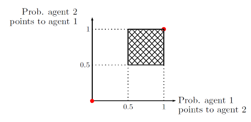
Figure 1: Weakly payoff monotone profiles (shaded area) and empirical equilibria in TTC game with complete information when trade is efficient. Agents trade with probability one in the unique empirical equilibrium: the only Nash equilibrium that is in the closure of weakly payoff monotone behavior.

Our argument does not depend on the assumption of complete information. Consider the TTC game when information is summarized by a common prior. Since revealing her true preference is dominant, each agent with each possible type will reveal her preferences with probability at least $1/2$ in each weakly payoff monotone profile. Thus, in any limit of a sequence of weakly payoff monotone strategies, each agent reveals her true preference with probability at least $1/2$. Consequently, in each empirical equilibrium there is a lower bound on the probability with which each agent is truthful. Given the realization of agents’ types, each agent always believes the true payoff type of the other agent is possible. Then, in each empirical equilibrium of the TTC, whenever trade is efficient (for the true types of the agents), each agent will place positive probability on the other agent pointing to her. Consequently, in each empirical equilibrium of the TTC, given that an agent prefers to trade, this agent will point to the other agent with probability one whenever efficient trade is possible. Thus, each empirical equilibrium of the TTC obtains the truthful outcome with certainty.

For the second-price auction consider the complete information structure whose associated normal form game is presented in Table 1. Let $\varepsilon>0$ and $\sigma\equiv(\sigma_{A},\sigma_{B})$ be the pair of probability distributions on each agent’s action space defined as follows. Agent $A$ places $\varepsilon$ probability on $H$, $1/2$ on $M$ and $1/2-\varepsilon$ on $L$. Agent $B$ places $1-2\varepsilon$ probability on $H$, and $\varepsilon$ on each of the other two actions. For small $\varepsilon$ this profile is weakly payoff monotone. This can be easily seen in Fig. 2. Starting at the top left of the figure is $\sigma_{B}$. This distribution induces the expected payoffs for agent $A$ shown at the top right of the figure. Since $M$ is the unique weakly dominant strategy for agent $A$ and $\sigma_{B}$ is interior, the highest payoff for agent $A$ is achieved by $M$. Between $L$ and $H$, agent $A$ obtains a higher payoff with $L$, because with $H$ she ends up buying the object for a price above her value with positive probability. Thus, expected payoffs for agent $A$ are ordered exactly as $\sigma_{A}$, which is shown at the bottom right of Fig. 2. If agent $A$ plays $\sigma_{A}$, agent $B$’s expected utility is that shown at the bottom left of Fig. 2. Agent $B$’s utility is maximized at her unique weakly dominant strategy. Thus, differences in $\sigma_{B}$ reveal differences in expected utility. More precisely, agent $B$ playing $H$ with higher probability than both $M$ and $L$ is consistent with $H$ having higher expected payoff than both $M$ and $L$. As $\varepsilon$ vanishes, this profile converges to a Nash equilibrium in which agent $A$ randomizes between $M$ and $L$ with equal probability.

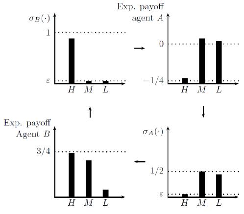
Figure 2: Weakly monotone distribution in the second price auction with complete information for agents $M$ and $H$. As $\varepsilon$ vanishes the distributions converge to a Nash equilibrium in which the lower value agent randomizes between $L$ and $M$.

Empirical equilibrium allows us to draw a clear difference between TTC and the second-price auction. Suppose that agents’ behavior is weakly payoff monotone. Then, if these mechanisms are operated, one will never observe that empirical distributions of play in TTC approximate an equilibrium producing a sub-optimal outcome. By contrast, this possibility is not ruled out for the second-price auction.

It turns out that these differences among these two mechanisms can be pinned down to a property that TTC satisfies and the second-price auction violates: non-bossiness in welfare-outcome, i.e., in the direct revelation game of the mechanism, an agent cannot change the outcome without changing her welfare (Theorem 1).

For the strategy-proof mechanisms that do violate non-bossiness, it is useful to examine which information structures produce undesirable empirical equilibria. It turns out that for a strategy-proof mechanism with essentially unique dominant strategies, like the second-price auction, this cannot happen for information structures with full support (Theorem 2). Thus, in a sense, our example above with the second-price auction actually requires the type of information structure we used.

Together, Theorems 1 and 2 produce sharp predictions about the type of behavior that is plausible when a strategy-proof scf is operated in different information structures. In Sec. 6 we review the relevant experimental and empirical literature and find that these predictions are consistent with it.

4 Model

A group of agents $N\equiv\{1,\dots,n\}$ is to select an alternative in an arbitrary set $X$. Agents have private values, i.e., each $i\in N$ has a payoff type $\theta_{i}$, determining an expected utility index $u_{i}(\cdot|\theta_{i}):X\rightarrow\mathbb{R}$. The set of possible payoff types for agent $i$ is $\Theta_{i}$ and the set of possible payoff type profiles is $\Theta\equiv\prod_{i\in N}\Theta_{i}$. We assume that $\Theta$ is finite. For each $S\subseteq N$, $\Theta_{S}$ is the cartesian product of the type spaces of the agents in $S$. The generic element of $\Theta_{S}$ is $\theta_{S}$. When $S=N\setminus\{i\}$ we simply write $\Theta_{-i}$ and $\theta_{-i}$. Consistently, whenever convenient, we concatenate partial profiles, as in $(\theta_{-i},\mu_{i})$. We use this notation consistently when operating with vectors (as in strategy profiles). We assume that information is summarized by a common prior $p\in\Delta(\Theta)$. For each $\theta$ in the support of $p$ and each $i\in N$, let $p(\cdot|\theta_{i})$ be the distribution $p$ conditional on agent $i$ drawing type $\theta_{i}$.

A social choice function (scf) selects a set of alternatives for each possible state. The generic scf is $g:\Theta\rightarrow X$. Three properties of scfs play an important role in our results. An scf $g$,

1. is strategy-proof if for each $\theta\in\Theta$, each $i\in N$, and each $\tau_{i}\in\Theta_{i}$, $u_{i}(g(\theta)|\theta_{i})\geq u_{i}(g(\theta_{-i},\tau_{i})|\theta_{i})$.

2. is non-bossy in welfare-outcome if for each $\theta\in\Theta$, each $i\in N$, and each $\tau_{i}\in\Theta_{i}$, $u_{i}(g(\theta)|\theta_{i})=u_{i}(g(\theta_{-i},\tau_{i})|\theta_{i})$ implies that $g(\theta)=g(\theta_{-i},\tau_{i})$.

3. has essentially unique dominant strategies if for each $\theta\in\Theta$, each $i\in N$, and each $\tau_{i}\in\Theta_{i}$, if $u_{i}(g(\theta)|\theta_{i})=u_{i}(g(\theta_{-i},\tau_{i})|\theta_{i})$ and $g(\theta)\neq g(\theta_{-i},\tau_{i})$, then there is $\tau_{-i}\in\Theta_{-i}$ such that $u_{i}(g(\tau_{-i},\theta_{i})|\theta_{i})>u_{i}(g(\tau)|\theta_{i})$.

The first property is well-known. The second property requires that no agent, when telling the truth (in the direct revelation mechanism associated with the scf), be able to change the outcome by changing her report without changing her welfare. It is satisfied, among other, by TTC, the Median Voting rule, and the Uniform rule. It is a strengthening of the non-bossiness condition of Satterthwaite and Sonnenschein (1981), which applies only to environments with private consumption. Non-bossiness in welfare-outcome is violated by the Pivotal mechanism, the second-price auction, and SPDA. The third property requires that any consequential deviation from a truthful report by an agent, can have adverse consequences for her. Restricted to strategy-proof scfs, this property says that, in the direct revelation game associated with the scf, for each agent, all dominant strategies are redundant. This is satisfied whenever true reports are the unique dominant strategies, as in the second-price auction. It is not necessary that dominant strategies be unique for this property to be satisfied. A student in a school choice environment with strict preferences, and in which SPDA is operated, may have multiple dominant strategies (think for instance of a student who is at the top of the ranking of each school). However, any misreport that is also a dominant strategy for this student, cannot change the outcome (see Online Appendix for a formal argument).

A mechanism is a pair $(M,\varphi)$ where $M\equiv(M_{i})_{i\in N}$ is an unrestricted message space and $\varphi:M\rightarrow\Delta(X)$ is an outcome function. A finite mechanism is that for which each $M_{i}$ is a finite set. Given the common prior $p$, $(M,\varphi)$ determines a standard Bayesian game $\Gamma\equiv(M,\varphi,p)$. When the prior is degenerate, i.e., places probability one in a payoff type $\theta\in\Theta$, we refer to this as a game of complete information and denote it simply by $(M,\varphi,\theta)$. A (behavior) strategy for agent $i$ in $\Gamma$ is a function that assigns to each $\theta_{i}\in\Theta_{i}$ that happens with positive probability under $p$, a function $\sigma_{i}(\cdot|\theta_{i})\in\Delta(M_{i})$. We denote a profile of strategies by $\sigma\equiv(\sigma_{i})_{i\in N}$. For each $S\subseteq N$, and each $\theta_{S}\in\Theta_{S}$, $\sigma_{S}(\cdot|\theta_{S})$ is the corresponding product measure $\prod_{i\in S}\sigma_{i}(\cdot|\theta_{i})$. When $S=N$ we simply write $\sigma(\cdot|\theta)$. We denote the measure that places probability one on $m_{i}\in M_{i}$ by $\delta_{m_{i}}$. With a complete information structure we simplify notation and do not condition strategies on an agent’s type, which is uniquely determined by the prior. Thus, in game $(M,\varphi,\theta)$ we write $\sigma_{i}$ instead of $\sigma_{i}(\cdot|\theta_{i})$.

Let $\theta_{i}\in\Theta_{i}$ be realized with positive probability under $p$. The expected utility of agent $i$ with type $\theta_{i}$, in $\Gamma$ from playing strategy $\mu_{i}$ when the other agents select actions as prescribed by $\sigma_{-i}$ is

$$U_{\varphi}(\sigma_{-i},\mu_{i}|p,\theta_{i})\equiv\sum u(\varphi(m)|\theta_{i})p(\theta_{-i}|\theta_{i})\sigma_{-i}(m_{-i}|\theta_{-i})\mu_{i}(m_{i}|\theta_{i}),$$

where the summation is over all $\theta_{-i}\in\theta_{-i}$ and $m\in M$. A profile of strategies $\sigma$ is a Bayesian Nash equilibrium of $\Gamma$ if for each $\theta\in\Theta$ in the support of $p$, each $i\in N$, and each $\mu_{i}\in\Delta(M_{i})$, $U_{\varphi}(\sigma_{-i},\mu_{i}|p,\theta_{i})\leq U_{\varphi}(\sigma_{-i},\sigma_{i}|p,\theta_{i})$. The set of Bayesian Nash equilibria of $\Gamma$ is $N(\Gamma)$. We say that $m_{i}\in M_{i}$ is a weakly dominant action for agent $i$ with type $\theta_{i}\in\Theta_{i}$ in $(M,\varphi)$ if for each $r_{i}\in M_{i}$, and each $m_{-i}\in M_{-i}$, $u_{i}(m|\theta_{i})\geq u_{i}(m_{-i},r_{i}|\theta_{i})$.

Our main basis for empirical plausibility of behavior is the following weak form of rationality.

Definition 1.

A profile of strategies for $\Gamma\equiv(M,\varphi,p)$, $\sigma\equiv(\sigma_{i})_{i\in N}$, is weakly payoff monotone for $\Gamma$ if for each $\theta\in\Theta$ in the support of $p$, each $i\in N$, and each pair $\{m_{i},n_{i}\}\subseteq M_{i}$ such that $\sigma_{i}(m_{i}|\theta_{i})>\sigma_{i}(n_{i}|\theta_{i})$, $U_{\varphi}(\sigma_{-i},\delta_{m_{i}}|p,\theta_{i})>U_{\varphi}(\sigma_{-i},\delta_{n_{i}}|p,\theta_{i})$.

We then identify the Nash equilibria that can be approximated by empirically plausible behavior.

Definition 2.

An empirical equilibrium of $\Gamma\equiv(M,\varphi,p)$ is a Bayesian Nash equilibrium of $\Gamma$ that is the limit of a sequence of weakly payoff monotone distributions for $\Gamma$.

In any finite game, proper equilibria (Myerson, 1978), firm equilibria and approachable equilibria (van Damme, 1991), and the limiting logistic equilibrium (McKelvey and Palfrey, 1995) are empirical equilibria. Thus, existence of empirical equilibrium holds for each finite game.

5 Results

We start with a key lemma stating that, when available, weakly dominant actions will always be part of the support of each empirical equilibrium in a game.

Lemma 1.

Let $(M,\varphi)$ be a mechanism and $p$ a common prior. Let $i\in N$ and $\theta_{i}\in\Theta_{i}$. Suppose that $m_{i}\in M_{i}$ is a weakly dominant action for agent $i$ with type $\theta_{i}$ in $(M,\varphi)$. Let $\sigma$ be an empirical equilibrium of $(M,\varphi,p)$. Then, $m_{i}$ is in the support of $\sigma_{i}(\cdot|\theta_{i})$.

The following theorem characterizes the strategy-proof scfs for which the empirical equilibria of its revelation game produce with certainty, for each common prior information structure, the truthful outcome.

Theorem 1.

Let $g$ be an scf. The following statements are equivalent.

1. For each common prior $p$ and each empirical equilibrium of $(\Theta,g,p)$, say $\sigma$, we have that for each pair $\{\theta,\tau\}\subseteq\Theta$ where $\theta$ is in the support of $p$ and $\tau$ is in the support of $\sigma(\cdot|\theta)$, $g(\theta)=g(\tau)$.

2. $g$ is strategy-proof and non-bossy in welfare-outcome.

We now discuss the proof of Theorem 1. Let us discuss first why a strategy-proof and non-bossy in welfare-outcome scf $g$ has the robustness property in statement 1 in the theorem. Suppose that $\sigma\in N(\Theta,g,p)$, that the true type of the agents is $\theta$, and that the agents end up reporting $\tau$ with positive probability under $\sigma$. Consider an arbitrary agent, say $i$. Since $g$ is strategy-proof, $\tau_{i}$ can be a best response for agent $i$ with type $\theta_{i}$ only if it gives the agent the same utility as reporting $\theta_{i}$ for each report of the other agents that agent $i$ believes will be observed with positive probability. Thus, since there are rational expectations in a common prior game, report $\tau_{i}$ needs to give agent $i$ the same utility as $\theta_{i}$ when the other agents report $\tau_{-i}$. Since $g$ is non-bossy in welfare-outcome, it has to be the case that $g(\tau_{-i},\theta_{i})=g(\tau)$. By Lemma 1, if $\sigma$ is an empirical equilibrium of $(\Theta,g,p)$, agent $i$ reports her true type with positive probability in $\sigma$. Thus, $(\tau_{-i},\theta_{i})$ is played with positive probability in $\sigma$. Thus, we can iterate over the set of agents and conclude that $g(\theta)=g(\tau)$.

Let us discuss now the proof of the converse statement. First, we observe that it is well-known that the type of robust implementation in statement 1 of the theorem implies the scf is strategy-proof (Dasgupta et al., 1979; Bergemann and Morris, 2005). Thus, it is enough to prove that if $g$ is strategy-proof and satisfies the robustness property, it has to be non-bossy in welfare-outcome. Our proof of this statement is by contradiction. We suppose to the contrary that for some type $\theta$, an agent, say $i$, can change the outcome of $g$ by reporting some alternative $\tau_{i}$ without changing her welfare. We then show that the complete information game $(\Theta,g,\theta)$ has an empirical equilibrium in which $(\theta_{-i},\tau_{i})$ is observed with positive probability. The subtlety of doing this resides in that our statement is free of details about the payoff environment in which it applies. We have an arbitrary number of agents and we know little about the structure of agents’ preferences. If we had additional information about the environment, as say for the second-price auction, the construction could be greatly simplified as in our illustrating example.

To solve this problem we design an operator that responds to four different types of signals, $\kappa^{\varepsilon,r,\eta,\lambda}:\Delta(\Theta_{1})\times\dots\times\Delta(\Theta_{n})\rightarrow\Delta(\Theta_{1})\times\dots\times\Delta(\Theta_{n})$, where $\{r,\lambda\}\subseteq\mathbb{N}$ and $\{\varepsilon,\eta\}\subseteq(0,1)$. This operator has fixed points that are always weakly payoff monotone distributions for $u$. For a given $\varepsilon$, the operator restricts its search of distributions to those that place at least probability $\varepsilon$ in each action for agent $i$. For a given $\eta$, the operator restricts its search of distributions to those that place at least probability $\eta$ in each action for each agent $j\neq i$. If we take $r$ to infinity, the operator looks for distributions in which agent $i$’s frequency of play is almost a best response to the other agents’ distribution (constrained by $\varepsilon$). If we take $\lambda$ to infinity, the operator looks for distributions in which for each agent $j\neq i$, her frequency of play is almost a best response to the other agents’ distribution (constrained by $\eta$). The proof is completed by proving that for the right sequence of signals, the operator will have fixed points that in the limit exhibit the required properties. To simplify our discussion without losing the core of the argument, let us suppose that each agent $j\neq i$ has a unique weakly dominant action for each type. Fix $\varepsilon$ and $r$. Since we base the construction of our operator on continuous functions, one can prove that there is $\delta>0$ such that for each fixed point of the operator, if the expected utility of reports $\theta_{i}$ and $\tau_{i}$ does not differ in more than $\delta$, then agent $i$ places probability almost the same on these two reports. Let $\eta>0$. If each agent $j\neq i$ approximately places probability $\eta$ in each action that is not weakly dominant and the rest in her dominant action, the utility of agent $i$ from reports $\theta_{i}$ and $\tau_{i}$ will be almost the same when $\eta$ is small. Thus, one can calibrate $\eta$ for this difference to be less than $\delta>0$. Let $\eta(\varepsilon,r,\delta)$ be this value. If we take $\lambda$ to infinity keeping $\varepsilon,r,\eta(\varepsilon,r,\delta)$ constant, the distribution of each agent $j\neq i$ in each fixed point of the operator will place, approximately, probability $\eta(\varepsilon,r,\delta)$ in each action that is not weakly dominant. Thus, for large $\lambda$, $\kappa^{\varepsilon,r,\eta(\varepsilon,r,\delta),\lambda}$ has a fixed point in which agent $i$ is playing $\theta_{i}$ and $\tau_{i}$ with almost the same probability and all other agents are playing their dominant strategy with almost certainty. We grab one of this distributions. It is the first point in our sequence, which we construct by repeating this argument starting from smaller $\varepsilon$s and $\delta$s and larger $r$s.

Interestingly, the conclusions of Theorem 1 depend on our requirement that the empirical equilibria of the scf generate only truthful outcomes for type spaces in which an agent may know, with certainty, the payoff type of the other agents.

Theorem 2.

Let $g$ be an scf. The following statements are equivalent.

1. For each full-support prior $p$ and each empirical equilibrium of $(\Theta,g,p)$, say $\sigma$, we have that for each pair $\{\theta,\tau\}\in\Theta$ where $\tau$ is in the support of $\sigma(\cdot|\theta)$, $g(\theta)=g(\tau)$.

2. $g$ is strategy-proof and has essentially unique dominant strategies.

Lemma 1 and Theorems 1 and 2 give us a clear description of the weakly payoff monotone behavior that can be observed when a strategy-proof scf is operated. In the next section we contrast these predictions with experimental evidence on strategy-proof mechanisms.

6 Experimental and empirical evidence

6.1 Dominant strategy play

The performance of strategy-proof mechanisms in an experimental environment has attracted a fair amount of attention. Essentially, experiments have been run to test the hypothesis that dominant strategy equilibrium is a reasonable prediction for these games. The common finding is a lack of support for this hypothesis in most simultaneous move dominant strategy mechanisms.

Our results provide an alternative theoretical framework from which one can reevaluate these experimental results. Theorems 1 and 2 state that as long as empirical distributions of play are weakly payoff monotone we should expect two features in data. First, we will never see agents’ behavior approximate a Nash equilibrium that is not truthful equivalent in two situations: (i) the scf is strategy-proof and non-bossy in welfare-outcome; or (ii) each agent believes all other payoff types are possible and the scf has essentially unique dominant strategies. Second, one cannot rule out that sub-optimal equilibria are approximated by weakly payoff monotone behavior when the scf violates non-bossiness in welfare-outcome and information is complete.

It is informative to note that our first conclusion still holds if we only require, instead of weak payoff monotonicity, that there is a lower bound on the probability with which an agent reports truthfully, an easier hypothesis to test. Thus, in order to investigate whether a sub-optimal Nash equilibrium is approximated in situations (i) and (ii), it is enough to verify that truthful play is non-negligible and does not dissipate in experiments with multiple rounds. This is largely supported by data.

In Table LABEL:Tab:Frq-dom-st, we survey the literature for experimental results with dominant strategy mechanisms. We find ten studies across a variety of mechanisms. In all of these studies we are able to determine, based on the number of pure strategies available to each player, how often a dominant strategy would be played if subjects uniformly played all pure strategies. In every experiment, rates of dominant strategy play exceed this threshold. A simple binomial test—treating each of these nine papers as a single observation—rejects any null hypothesis that these rates of dominant strategy play are drawn from a random distribution with median probability at or below these levels ($p<0.001$). Thus one would reasonably conclude that rates of dominant strategy play should exceed that under uniform support.

It is evident then that the accumulated experimental data supports the conclusion that under conditions (i) and (ii) agents’ behavior is not likely to settle on a sub-optimal equilibrium. As long as agents are not choosing a best response, the behavior of the other agents will continue flagging their consequential deviations from truthful behavior as considerably inferior.

6.2 Observing empirical equilibria

Among the experiments we surveyed, Cason et al. (2006), Healy (2006), and Andreoni et al. (2007) involve the operation of a strategy-proof mechanism that violates non-bossiness in welfare-outcome in an information environment in which information is not interior. These experiments offer us the chance to observe Nash equilibria attaining outcomes different from the truthful one with positive probability.

In Cason et al. (2006), two-agent groups (row and column) play eight to ten rounds in randomly rematched groups with the same pivotal mechanism payoff matrix over all rounds. This experiment was designed to test “secure implementation” (Saijo et al., 2007). This theory obtains a characterization of scfs whose direct revelation game implements the scf itself both in dominant strategies and Nash equilibria for all complete information priors. By running experiments with the pivotal mechanism, which violates the secure implementation requirements, the authors illustrated that this may be compatible with the observation of equilibria that are not truthful equivalent. Indeed, these authors argue that even though deviations from dominant strategy play are arguably persistent in their pivotal mechanism experiment, virtually all subjects are playing mutual best responses to the population of subjects by the end of the experiment (c.f., Figure 7, Cason et al., 2006).

In Healy (2006), five-agent groups with fixed utility functions play fifty rounds in a mechanism that belongs to the VCG family to choose the level of provision of a public good. Agents have quasi-linear preferences and their utility for the public good is determined by two parameters. Since it is central to his analysis, the author directly addresses the issue and concludes that “weakly dominated $\varepsilon$-Nash equilibria are observed, while the dominant strategy equilibrium is not” (Result 4 Healy, 2006).

In Andreoni et al. (2007), groups of four agents sequentially play three simultaneous games in each round for thirty rounds. Groups are rematched each round and play an auction game with the same values but increasing precision of information about the other players. The first game involves no information about the other players’ valuations beyond the distribution from which they are drawn. The final game involves complete information. These authors run separate sessions with the first-price auction and the second-price auction.

Andreoni et al. (2007)’s main objective is to experimentally evaluate the effect of information structure on the first-price and second-price auctions. Their theoretical benchmark is the information-driven comparative statics developed by Kim and Che (2004) for the first-price auction, and the dominant strategy hypothesis, which implies there is no role of information structure, for the second-price auction. Thus, these authors designed and carried out an ideal experiment to evaluate the operation of a bossy strategy-proof scf that has unique dominant strategies, the second-price auction, in both full-support and complete information environments. In contrast to the dominant strategy hypothesis, empirical equilibrium analysis has sharp predictions for such a mechanism in these environments.

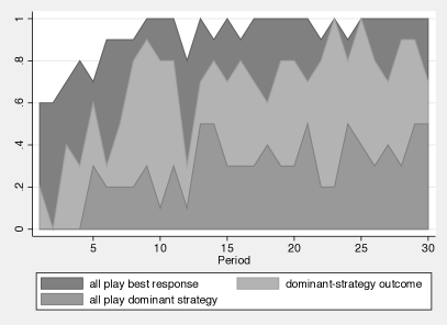
Figure 3: Group outcomes in 4-person, second-price auctions in Andreoni et al. (2007) under full-support incomplete (left) and complete (right) information. The dark gray area indicates the proportion of outcomes where all subjects play mutual best responses to the actions of all other group members. The light gray area indicates outcomes where the transaction associated with the dominant strategy outcome occurs, that is, the subject with the highest valuation obtains the item and pays the amount of the second highest valuation. The medium gray area indicates the percentage of group outcomes where all subjects play a dominant strategy. Note that each level necessarily contains the subsequent level. Subjects are rematched randomly across a group of 20 each period.

One can argue that frequencies of play in all treatments in Andreoni et al. (2007)’s experiment accumulate towards a Nash equilibrium. Fig. 3 shows the proportion of outcomes where all subjects in a group play best-responses (dark gray), where the subject with the highest valuation obtains it at the second highest valuation (light gray), and all subjects play dominant strategies (medium gray) under full-support incomplete information (left) and complete information (right). In both cases, virtually all subjects are playing mutual best responses to the population of subjects in the second half of the experiment. Note that frequencies of best response play plotted in Fig. 3 are the percentage of groups in which all four agents end up playing a best response to each other. Even when this percentage is 80%, individual rates of best response play is about 95%.

Empirical equilibrium analysis reveals that behavior that is weakly payoff monotone and approximates mutual best responses in this experiment will necessarily have certain characteristics. For the second-price auction if information is interior, as in the first information treatment, this type of behavior can only approximate a truthful equivalent Nash equilibrium. If information is complete, as in the last information treatment, this type of behavior can accumulate towards a Nash equilibrium in which the lower value agents randomize with positive probability. Both phenomena are supported by the data.

Fig. 4 allows us to understand behavior in both information structures. The figure standardizes bids to valuations (the highest valuation is assigned a value of 4, the second highest a value of 3, and so on) and shows the median bid and the range that contains the higher and lower 85% of bids for bids by each of the four ranked valuation types. In both treatments the median bid for any of the four types generally falls on its respective valuation, consistent with dominant strategy play.

In the full-support incomplete information treatment, agents’ deviations from their dominant strategies do not induce consequential deviations from the truthful equilibrium. After the initial five rounds, median bids are the agents’ own values (Fig. 4 (left)). In the last twenty five rounds, 74.4% outcomes are truthful (Fig. 3 (left)); 97.2% outcomes are efficient, i.e., such that a highest valuation agent wins the auction (Fig. 5 (left)); in 94.4% of outcomes the price is determined by the bid of a second valuation agent; and on average the price paid by the winner differs in 1.188 points (average of the absolute value of differences) from the second highest valuation (Fig. 5 (right)). Thus, the mechanism is arguably achieving the social planner’s objectives. It is virtually assigning the good to a highest valuation agent and it is essentially raising revenue equal to the second highest valuation.

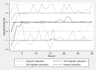
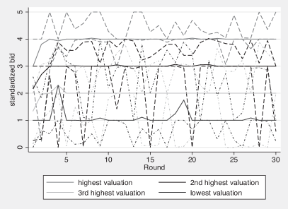
Figure 4: Median bid and 15th-85th percentile range by valuation type in 4-person, second-price auctions of Andreoni et al. (2007) under incomplete (left) and complete (right) information. Bids are standardized so that the valuation of the 1st-4th valuations in the specific auction are assigned values 4–1, respectively. Bids of 100 (the highest possible valuation) and 200 (the highest possible bid) are assigned values of 5 and 6, respectively. If two valuation types have the same value, valuation order is randomly assigned. Bids between two valuations are standardized by $(bid-valuation_{j})/(valuation_{i}-valuation_{j})$ where $i$ is the highest valuation a bid exceeds and $j$ is the next highest valuation. Bids below the lowest valuation are standardized on the interval between 0 and the lowest valuation. Bids above the highest valuation are standardized either on the interval between the highest valuation and 100 (values of 4–5), or 100 and 200 (values of 5–6). For example, for the four valuations 80, 40, 25, 10, bids of 150, 40, 30, and 5 would be 5.5, 3, 2.33, and 0.5, respectively.

In the complete information treatment, after five rounds median bids are also the agents’ own values (Fig. 4 (right)). Differently from the incomplete information case, deviations from truthful behavior do not dissipate and are consequential. In the last twenty five rounds, 38.4% outcomes are truthful (Fig. 3 (right)); 91.6% outcomes are efficient, i.e., such that a highest valuation agent wins the auction (Fig. 5 (left)); in 68.4% of outcomes the price is determined by the bid of a second valuation agent; and on average the price paid by the winner differs in 8.704 points from the second highest valuation (Fig. 5 (right)). Thus, even though the mechanism is assigning the good to the right agent, it is raising a revenue that is persistently away from the social planner’s objective.

A simple reason explains the differences in behavior between treatments. Under incomplete information there is a penalty for a player to deviate too much from his/her dominant strategy. There is no corresponding penalty under complete information. As long as a lower valuation player does not outbid the first, the payoff of the lower valuation agent will be zero regardless. Together these experiments reveal that agents do react to pecuniary incentives and use information and observed frequencies of play of the other agents in a meaningful way. They do not preemptively react to a hypothetical tremble of the other agents, however. In the complete information case the highest valuation agent persistently overbids and the other agents persistently bid on a wide range under the highest valuation agent’s value. As long as these behaviors are essentially separated, they are mutual best responses. On the other hand, in the incomplete information treatment, for each bid, there is a positive probability that at least an agent draws that bid as valuation. Since agents bid their values with high probability (68.2% on average), there is a non-trivial chance that a significant deviation from truthful behavior is suboptimal. Thus, agents take into account a potential loss in utility, but only when there is an actual significant probability of it being realized.

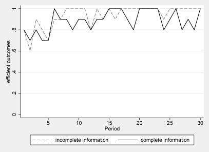
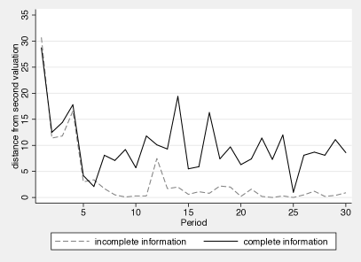
Figure 5: Frequency of efficient outcomes (left) and average distance (conditional on efficient outcome) between the price and a second valuation (right) in the second-price auction experiments of Andreoni et al. (2007) in the full-support incomplete and complete information treatments.

6.3 Payoff monotonicity

One of the advantages of empirical equilibrium analysis is that it is based on an observable property of behavior. That is, the conclusions of our theorems will hold whenever empirical distributions are weakly payoff monotone. Thus, evaluating the extent to which agents frequencies of play satisfy this property allows us to understand better the positive content of our theory.

Evaluating weak payoff monotonicity is an elusive task, however. In realistic games as those in the experiments we surveyed, action spaces and type spaces are large (e.g., Attiyeh et al., 2000 has 2001 actions). This makes the data requirements for fully testing payoff monotonicity unrealistic. It is plausible that data can point to differences on frequencies of play between two given actions for a certain agent type. In order to test that this is consistent with weak payoff monotonicity one would need to verify that the expected payoffs of these actions given what the other agents are doing are ranked in accordance to the frequencies of play of these actions. Doing so requires, in most cases, that one has a good estimate of the whole distribution of play for all agent types.

Even though fully testing weak payoff monotonicity is not feasible with realistic data sets, one can test for certain markers of this property that are less demanding on data. First, in weakly payoff monotone data sets there should be a positive association between the frequencies with which actions are played and their empirical expected utility. For the four studies where we have sufficient data (Andreoni et al., 2007; Attiyeh et al., 2000; Cason et al., 2006; Li, 2017), we can compare the actual payoffs earned with each action choice with the counterfactual payoffs had a subject chosen a different action. If subjects choose actions independent of payoffs—a gross violation of weak monotonicity—we should suspect the differences between the average payoffs of played strategies and counterfactual payoffs of non-played strategies to be evenly distributed around zero. Instead we find in all cases the average payoffs of played strategies exceed those of non-played strategies. Treating the 30 total sessions across these four studies as independent observations, we can easily reject the null hypothesis that strategies are played independent of expected payoffs $(p<0.001)$.

Not all features of data are in line with weak payoff monotonicity, however. We are aware of three of these. First, in the Pivotal mechanism experiment of Cason et al. (2006), there are two dominant strategies for each agent. While the Column agent chooses them with similar frequencies (36.1% and 38.3%), the Row agent chooses them with frequencies 51.1% and 19.4%. Parametric paired t-tests and non-parametric signed rank and sign tests suggest the later difference is statistically significant at the subject level $(p<0.01)$, but not the former. Second, there is a well documented propensity of overbidding in second-price auctions. This does not have to be necessarily at odds with weak payoff monotonicity. Agents who draw larger values will find overbidding with respect to value to be a less costly mistake than underbidding. Low value agents will have fewer bids below their value than above their value. Thus, such an agent’s distribution of play can still be weakly payoff monotone and in aggregate overbid more than underbid. However, Figure 1 in Andreoni et al. (2007), which depicts the frequency of the difference between the bid of the low value agents and the maximal value, shows that these agents place significantly higher weight in the bids that are close to the maximal value agent. This is a clear violation of weak payoff monotonicity, which as Andreoni et al. (2007) argue, may have origin in spiteful behavior of the low value agents. Finally, a simple behavioral regularity as rounding to multiples of five, can easily induce violations of weak payoff monotonicity (such patterns are present in the auction data of Andreoni et al., 2007; Brown and Velez, 2019; Li, 2017, for instance).

In order to evaluate the positive content of empirical equilibrium analysis, it is necessary to understand the consequences for our analysis of these and other possible violations of weak payoff monotonicity. One avenue is to reconsider our construction and restart from a more basic principle than weak payoff monotonicity. Observe that this property can be stated in its contrapositive form as follows: If between two actions, say $a$ and $b$, an agent’s expected utility of $a$ given what the other are doing is greater than or equal to that of $b$, then the frequency with which the agent plays $a$ should be no less than the frequency with which the agent plays $b$. Stated in this form this property can be naturally weakened as follows. One can require the existence of some constant $\alpha\in(0,1)$ such that for any two actions available to an agent, say $a$ and $b$, if the expected utility of $a$ given what the other are doing is greater than or equal than that of $b$, then the frequency with which the agent plays $a$ should be no less than $\alpha$ times the frequency with which the agent plays $b$. One can determine that all our results follow through if we take as basis for plausibility this weaker property. It is interesting in itself to see that such a weak property still provides empirical restrictions on data. Moreover, the main message of empirical equilibrium analysis in other applications, like full implementation, is also preserved under this generalization (Velez and Brown, 2019b).

We prefer to maintain the analysis based on weak payoff monotonicity because it strikes a balance between the regularity it provides while being challenged only by phenomena that (i) do not seem universally relevant, and (ii) seem to induce only continuous violations of this principle. Agents may round their bids, may be attracted by labels attached to certain actions, may exhibit other regarding preferences in certain contexts, and so on. At the end, what matters for empirical equilibrium analysis is that these features of behavior will be part of a bigger scheme in which agents are to a significant extent trying to hit their best payoffs given what the other agents are doing. By analyzing what happens when these less well understood effects are absent, we obtain a powerful benchmark producing policy relevant comparative statics.

Finally, an emerging empirical literature concerning strategy-proof mechanisms presents evidence in line with the predictions of empirical equilibrium. In empirical data, in which payoff types are not observable, it is of course challenging to determine what a deviation from truthful behavior is. However, in some instances the researcher is able to identify dominated actions, as an agent refusing to apply for financial support when this does not influence her acceptance to an academic position (Hassidim et al., 2020) or by means of ex-post surveys (Rees-Jones, 2017). The common finding is that these types of reports are observed with positive probability. However, in line with our results, they are more common among the agents for whom they are less likely to be consequential (Hassidim et al., 2020; Rees-Jones, 2017; Artemov et al., 2020; Chen and Pereyra, 2019; Shorrer and Sóvágó, 2019).

7 Robust mechanism design and revelation principle

One can draw an informative parallel between our results and the robust full implementation of scfs (Bergemann and Morris, 2005). This literature articulates the idea that the designer should look for mechanisms that operate well independently of informational assumptions. Of course one’s judgement about this depends on the prediction that one uses. Here are the news if one considers the Nash equilibrium prediction.

Theorem 3.

Let $g$ be an scf. The following are equivalent.

1. There is a finite mechanism $(M,\varphi)$ such that for each possible common prior $p$, each Bayesian Nash equilibrium $\sigma$ of $(M,\varphi,p)$, each possible $\theta\in\Theta$ in the support of $p$, and each message $m$ in the support of $\sigma(\cdot|\theta)$, $\varphi(m)=g(\theta)$.

2. (i) $g$ is strategy-proof and non-bossy in welfare-outcome, and (ii) $g$ satisfies the outcome rectangular property, i.e., for each pair of payoff types $\{\theta,\tau\}\subseteq\Theta$, if for each $i\in N$, $g(\theta_{i},\tau_{-i})=g(\tau)$, then $g(\theta)=g(\tau)$.

A parallel result to Theorem 3 is due to Saijo et al. (2007) ($1\Rightarrow 2$) and Adachi (2014) ($2\Rightarrow 1$) in an environment in which they restrict to pure-strategy equilibria and they consider implementation for type spaces larger than our payoff-type space. Our statement includes mixed-strategy equilibria and does not make any requirement for type spaces in which payoff types can be “cloned.” Thus, Saijo et al. (2007) and Adachi (2014)’s results do not trivially imply Theorem 3 by means of Bergemann and Morris (Sec. 6.3, 2011)’s purification argument. The proof of Theorem 3 can be completed by adapting the arguments in these papers, however. We include it in an online Appendix.

Theorem 3 allows us to make a precise comparison of Theorems 1 and 2 with the literature on robust implementation. As mentioned in the introduction, the conditions in Theorem 3 are restrictive (c.f. Saijo et al., 2007; Bochet and Sakai, 2010; Fujinaka and Wakayama, 2011). The outcome rectangular property is responsible for large part of these restrictions (Table 2). Thus, the aim of designing mechanisms that produce only the desired outcomes, in all Nash equilibria for all information structures, may be unnecessarily pessimistic. None of the mechanisms in Table 2 pass the test. However, if one already believes that a Nash equilibrium will be a good prediction when the mechanism is operated, it is enough to be concerned only with the Nash equilibria that is plausible will be observed. By Theorem 1, TTC, Uniform rule, and median voting pass the more realistic test for all common prior type spaces. By Theorem 2, the second-price auction, Pivotal mechanism, and SPDA pass the test for all full-support common prior type spaces.

scf	Strategy proofness	Essentially unique dominant strategies	Non-bossiness in welfare-outcome	outcome rectangular property
TTC	$+$	$+$	$+$	$-$
Uniform rule	$+$	$+$	$+$	$-$
Median voting	$+$	$+$	$+$	$-$
Second price auction	$+$	$+$	$-$	$-$
Pivotal	$+$	$+$	$-$	$-$
SPDA	$+$	$+$	$-$	$-$

Table 2: Strategy-proof scfs and the outcome rectangular property; $+$ indicates that the property labeling the column is satisfied by the scf, and $-$ the opposite. These statements refer to the usual preference spaces in which these scfs are defined.

It is worth noting that statement 1 in Theorem 3 is quantified over all finite mechanisms, while statement 1 in Theorem 1 only refers to the direct revelation game of the scf. It turns out that whenever statement 1 in Theorem 3 is satisfied by some mechanism for an scf, it is also satisfied by the scf’s direct revelation mechanism (Saijo et al., 2007). This means that a “revelation principle” holds for this type of implementation.

It is not clear that a revelation principle holds when empirical equilibrium is one’s prediction in these games. That is, we do not know whether there is a strategy-proof scf that violates non-bossiness in welfare-outcome for which there is a mechanism that has the properties in statement 1 of Theorem 1. The issue is very interesting and subtle.

It is known that the restriction to direct revelation mechanisms is not without loss of generality for full implementation. That is, dominant strategy full implementation may require richer message spaces than the payoff-type spaces (Dasgupta et al., 1979; Repullo, 1985). Strikingly, Repullo (1985) constructs a finite social choice environment that admits a strategy-proof social choice function whose direct revelation game for certain type has a dominant strategy equilibrium that Pareto dominates the outcome selected by the scf for that type. Moreover, the social choice environment in this example also admits a mechanism that implements in dominant strategies the social choice function.

By Lemma 1 we know that a dominant strategy profile in a game will always be observed with positive probability in each empirical equilibrium of the game. Thus, Repullo (1985)’s concern that undesirable outcomes —in this case dominant strategy equilibrium outcomes— of a direct revelation game for a strategy-proof scf may be empirically plausible, is well founded. As Repullo (1985) proves, it is possible to enlarge the message spaces and tighten the incentives for the selection of a particular outcome in a way that the desired outcome is the only dominant strategy outcome. It turns out that this type of message space enlargement, i.e., those that retain the existence of dominant strategies, will not resolve the issue for empirical equilibrium implementation.

Theorem 4 (Revelation principle for dominant strategy finite mechanisms).

Let $g$ be an scf. The following are equivalent.

1. There is a finite mechanism $(M,\varphi)$ for which each agent type has at least a weakly dominant action, and such that for each possible common prior $p$, each empirical equilibrium $\sigma$ of $(M,\varphi,p)$, each possible type $\theta\in\Theta$ in the support of $p$, and each message $m$ in the support of $\sigma(\cdot|\theta)$, $\varphi(m)=g(\theta)$.

2. For each common prior $p$ and each empirical equilibrium of $(\Theta,g,p)$, say $\sigma$, we have that for each pair $\{\theta,\tau\}\subseteq\Theta$ where $\theta$ is in the support of $p$ and $\tau$ is in the support of $\sigma(\cdot|\theta)$, $g(\theta)=g(\tau)$.

3. $g$ is strategy-proof and non-bossy in welfare-outcome.

Theorem 4 implies that it is impossible to obtain robust implementation in empirical equilibrium of a social choice function that violates non-bossiness in welfare-outcome by a dominant strategies mechanism. It is worth noting that enlarging the message space on the direct revelation game of a strategy-proof scf that violates non-bossiness in welfare-outcome may have a meaningful effect on the performance of the mechanism, even when one preserves the existence of dominant strategies.

Example 1.

Consider an environment with two agents $N\equiv\{1,2\}$ whose payoff-type spaces are $\Theta_{1}\equiv\{\theta_{1}\}$ and $\Theta_{2}\equiv\{\theta_{2},\theta_{2}^{\prime}\}$. There are two possible outcomes $\{a,b\}$; and $u_{1}(a|\theta_{1})>u_{1}(b|\theta_{1})$, $u_{2}(a|\theta_{2})=u_{1}(b|\theta_{2})$, and $u_{2}(a|\theta_{2}^{\prime})<u_{2}(b|\theta_{2}^{\prime})$. Suppose that a social planner desires to implement the efficient dictatorship in which agent $2$ gets her top choice. One can easily see that for any common prior $p$, for each empirical equilibrium of $(\Theta,g,p)$, say $\sigma$, agent $2$ with payoff type $\theta_{2}$ uniformly randomizes in $\Theta_{2}$. Thus, in each empirical equilibrium of $(\Theta,g,p)$, agent $2$ always achieves her top choice and agent $1$ receives her top choice with $1/2$ probability when this does not conflict with agent $2$’s preferences. Suppose now that the social planner uses mechanism $(M,\varphi)$ defined as follows: $M_{1}\equiv\{\theta_{1}\}$, $M_{2}\equiv\{\theta_{2}^{\prime},m_{2}^{1},....,m_{2}^{k}\}$ where $k\in\mathbb{N}$, $\varphi(\theta_{1},\theta_{2}^{\prime})=b$, and for each $l=1,...,k$, $\varphi(\theta_{1},m_{2}^{l})=a$. One can see easily that in each empirical equilibrium of $(M,\varphi,p)$, agent $2$ always achieves her top choice and agent $1$ receives her top choice with $k/(k+1)$ probability when this does not conflict with agent $2$’s preferences.∎

Finally, it is well known that the restriction to social choice functions is not without loss of generality in robust implementation. Indeed, Bergemann and Morris (2005, Example 2) show that “partial” robust implementation can be achieved for a “social choice correspondence” that does not posses any strategy-proof single-valued selection. Their argument can be adapted to account for mixed strategies, which are essential in our analysis, and to show that the same phenomenon happens in our environment (see Example 2 in our Online Appendix).

8 Conclusion

We have presented theoretical and empirical evidence that strategy-proof scfs are not all the same with respect to how plausible it is that behavior in the direct revelation game associated with the scf can approximate a suboptimal equilibrium. Our analysis is based on empirical equilibrium, a refinement of Nash equilibrium that we introduce. It selects all the Nash equilibria that are not rejected as implausible by some model that is disciplined by weak payoff monotonicity. We draw two main conclusions under the hypothesis that observable behavior satisfies this property. First, behavior from the operation of a strategy-proof and non-bossy in welfare-outcome scf will never approximate a sub-optimal Nash equilibrium. Second, if the mechanism violates the non-bossiness condition but has essentially unique dominant strategies, then behavior can approximate a sub-optimal equilibrium only if information is not interior. These predictions are supported by experimental data on multiple mechanisms. The weak payoff monotonicity hypothesis fares well in data, but violations of it can be spotted in particular environments. These violations do not hinder the main conclusions of our study, however.

Appendix

Proof of Lemma 1.

Let $\Gamma\equiv(M,\varphi,p)$ and $\sigma\in N(\Gamma)$ be as in the statement of the lemma. Consider a sequence of weakly payoff monotone distributions for $\Gamma$, $\{\sigma^{\lambda}\}_{\lambda\in\mathbb{N}}$, such that for each $i\in N$ and each $\theta_{i}\in T_{i}$, as $\lambda\rightarrow\infty$, $\sigma^{\lambda}(\cdot|\theta_{i})\rightarrow\sigma(\cdot|\theta_{i})$. Let $\lambda\in\mathbb{N}$ and $m_{-i}\in M_{-i}$. Since $m_{i}$ is a weakly dominant action for agent $i$ with type $\theta_{i}$ in $(M,\varphi)$, for each $r_{i}\in M_{i}$, $u_{i}(\varphi(m_{-i},m_{i})|\theta_{i})\geq u_{i}(\varphi(m_{-i},r_{i})|\theta_{i})$. Thus, $U_{\varphi}(\sigma^{\lambda}_{-i},\delta_{m_{i}}|p,\theta_{i})\geq U_{\varphi}(\sigma^{\lambda}_{-i},\delta_{r_{i}}|p,\theta_{i})$. Since $\sigma$ is weakly payoff monotone for $\Gamma$, we have that for each $r_{i}\in M_{i}$, $\sigma^{\lambda}_{i}(m_{i}|\theta_{i})\geq\sigma^{\lambda}_{i}(r_{i}|\theta_{i})$. Convergence implies that $\sigma_{i}(m_{i}|\theta_{i})\geq\sigma_{i}(r_{i}|\theta_{i})$. Thus, $m_{i}$ is in the support of $\sigma_{i}(\cdot|\theta_{i})$. ∎

Proof of Theorems 1 and 4.

We prove Theorem 4, which implies Theorem 1. We first prove that statement 3 in the theorem implies statement 2. Suppose that $g$ is strategy-proof and non-bossy in welfare-outcome. Let $p$ be a common prior and $\sigma$ an empirical equilibrium of $(\Theta,g,p)$. Let $\theta\in\Theta$ be in the support of $p$. Thus, for each $i\in N$, $p(\theta_{-i}|\theta_{i})>0$. Let $\tau\in\Theta$ be in the support of $\sigma(\cdot|\theta)$, i.e., $\tau$ is a report that is observed with positive probability when the true types are $\theta$. Let $i\in N$. Since $\sigma\in N(\Theta,g,p)$, we have that

$$U_{g}(\sigma_{-i},\delta_{\tau_{i}}|p,\theta_{i})\geq U_{g}(\sigma_{-i},\delta_{\theta_{i}}|p,\theta_{i}).$$

Since $g$ is strategy-proof, the integrand of the expression on the right dominates point-wise the integrand of the expression on the left. Thus, the integrands are equal on the support of the common integrating measure. Notice that since $p(\theta_{-i}|\theta_{i})>0$ and $\tau$ is in the support of $\sigma(\cdot|\theta)$, agent $i$ assigns positive probability that the other agents profile of reports is $\tau_{-i}$. Thus, $u_{i}(g(\tau)|\theta_{i})=u_{i}(g(\tau_{-i},\theta_{i})|\theta_{i})$. Since $g$ is non-bossy in welfare-outcome,

$$g(\tau)=g(\tau_{-i},\theta_{i}).$$ (1)

By Lemma 1, $\theta_{i}$ is in the support of $\sigma_{i}(\cdot|\theta_{i})$. Thus, $(\tau_{-i},\theta_{i})$ is in the support of $\sigma(\cdot|\theta)$. Thus, the recursive argument shows that $g(\tau)=g(\theta)$.

We now prove that statement 2 implies statement 1. Since each empirical equilibrium is a Bayesian Nash equilibrium, statement 2 implies that for each common prior $p$ there is a Bayesian Nash equilibrium of $(\Theta,g,p)$ that obtains for each $\theta\in\Theta$, $g(\theta)$ with probability one. It is well known that this implies $g$ is strategy-proof (Dasgupta et al., 1979; Bergemann and Morris, 2005). Thus, $(\Theta,g)$ is a dominant strategies mechanism that satisfies the conditions in statement 1 of the theorem.

We now prove that statement 1 implies statement 3. Suppose that statement 1 is satisfied. That is, there is a finite mechanism $(M,\varphi)$ for which each agent type has at least a dominant strategy, and such that for each common prior $p$, each empirical equilibrium $\sigma$ of $(M,\varphi,p)$, each possible type $\theta\in\Theta$ in the support of $p$, and each message $m$ in the support of $\sigma(\cdot|\theta)$, $\varphi(m)=g(\theta)$.

We prove that $g$ is strategy-proof. For each $i\in N$ and $\theta_{i}\in\Theta_{i}$, let $m_{i}(\theta_{i})$ be a weakly dominant action for $i$ with type $\theta_{i}$ in $(M,\varphi)$. Let $p$ be a full-support common prior and $\sigma$ an empirical equilibrium of $(M,\varphi,p)$. By Lemma 1, for each $i\in N$ and $\theta_{i}\in\Theta_{i}$, $m_{i}(\theta_{i})$ is in the support of $\sigma(\cdot|\theta_{i})$. By statement 1, for each $\theta\in\Theta$, $\varphi(m(\theta))=g(\theta)$ (this means that $(M,\varphi)$ fully implements $g$ in dominant strategy equilibria, which by the usual revelation principle argument, which we spell out next, implies $g$ is strategy-proof). Let $\theta\in\Theta$, $i\in N$ and $\tau_{i}\in\Theta_{i}$. Since $m_{i}(\theta_{i})$ is a weakly dominant action for $i$ with type $\theta_{i}$ in $(M,\varphi)$, we have that $u_{i}(\varphi(m(\theta)|\theta_{i})\geq u_{i}(\varphi(m_{-i}(\theta_{-i}),m_{i}(\tau_{i}))|\theta_{i})$. Thus, $u_{i}(g(\theta)|\theta_{i})\geq u_{i}(g(\theta_{-i},\tau_{i})|\theta_{i})$. Thus, $g$ is strategy-proof.

We prove that $g$ is non-bossy in welfare-outcome. Suppose by contradiction that there is $\theta\in\Theta$, $i\in N$, and $\tau_{i}\in\Theta_{i}$ such that $u_{i}(g(\theta)|\theta_{i})=u_{i}(g(\theta_{-i},\tau_{i})|\theta_{i})$ and $g(\theta)\neq g(\theta_{-i},\tau_{i})$. Suppose without loss of generality that this agent is $i=1$. Let $a\equiv g(\theta)$ and $b\equiv g(\theta_{-1},\tau_{1})$. Again, for each $i\in N$ and $\theta_{i}\in\Theta_{i}$, let $m_{i}(\theta_{i})$ be a weakly dominant action for $i$ with type $\theta_{i}$ in $(M,\varphi)$. We claim that $m_{1}(\tau_{1})$ is a best response to $m_{-1}(\theta_{-1})$ for agent $i$ with type $\theta_{1}$, i.e., for each $m_{1}^{\prime}\in M_{1}$,

$$u_{1}(\varphi(m_{-1}(\theta_{-1}),m_{1}(\tau_{1}))|\theta_{1})\geq u_{1}(\varphi(m_{-1}(\theta_{-1}),m_{1}^{\prime})|\theta_{1}).$$ (2)

By Lemma 1, in each empirical equilibrium of $(M,\varphi,(\theta_{-1},\tau_{1}))$, $(m_{-1}(\theta_{-1}),m_{1}(\tau_{1}))$ is played with positive probability and in each empirical equilibrium of $(M,\varphi,\theta)$, $(m_{-1}(\theta_{-1}),m_{1}(\theta_{1}))$ is played with positive probability. Since $(M,\varphi)$ satisfies statement 1, $\varphi(m_{-1}(\theta_{-1}),m_{1}(\tau_{1}))=b$ and $\varphi(m_{-1}(\theta_{-1}),m_{1}(\theta))=a$. Since $m_{1}(\theta_{1})$ is a dominant strategy for agent $1$ with type $\theta_{1}$, we have that for each $m_{1}^{\prime}\in M_{1}$, $u_{1}(\varphi(m_{-1}(\theta_{-1}),m_{1}(\tau_{1}))|\theta_{1})=u_{1}(\varphi(m_{-1}(\theta_{-1}),m_{1}(\theta_{1}))|\theta_{1})\geq u_{1}(\varphi(m_{-1}(\theta_{-1}),m_{1}^{\prime})|\theta_{1})$. This is (2).

Consider the complete information game $(M,\varphi,\theta)$. Let $\sigma^{*}$ be the profile of strategies in $(M,\varphi,\theta)$ defined as follows. For each agent $j\neq 1$, $\sigma_{j}^{*}$ uniformly randomizes among $j$’s weakly dominant actions; agent $1$ uniformly randomizes among her best responses to $\sigma^{*}_{-1}$. (Recall that in a complete information game we do not condition strategies on agents’ types, i.e., $\sigma^{*}_{i}$ is the strategy of agent $i$ with type $\theta_{i}$.) Clearly, $\sigma^{*}$ is a Bayesian Nash equilibrium of $(M,\varphi,\theta)$. Since $m_{-1}(\theta_{-1})$ in (2) is an arbitrary profile of weakly dominant strategies for agents $N\setminus\{i\}$ with type $\theta_{-1}$ in $(M,\varphi)$, we have that for agent $i$ with type $\theta_{1}$, $m_{1}(\tau_{1})$ is a best response to $\sigma^{*}_{-1}$ in $(M,\varphi,\theta)$, i.e., for each $m_{1}^{\prime}\in M_{1}$,

$$U_{\varphi}(\sigma^{*}_{-i},\delta_{m_{1}(\tau_{1})}|\delta_{\theta_{-1}},\theta_{i})\geq U_{\varphi}(\sigma^{*}_{-i},\delta_{m^{\prime}_{1}}|\delta_{\theta_{-1}},\theta_{i}).$$

Thus, $(m_{-1}(\theta_{-1}),m_{1}(\tau_{1}))$ is in the support of $\sigma^{*}$. Thus, $\sigma^{*}$ is a Bayesian Nash equilibrium of $(M,\varphi,\theta)$ that obtains with positive probability outcome $b=\varphi(m_{-1}(\theta_{-1}),m_{1}(\tau_{1}))$ (when the agents’ type is $\theta$, which is the only element in the support of the prior).

The proof concludes by showing that $\sigma^{*}$ is an empirical equilibrium of $(M,\varphi,\theta)$, which contradicts statement 1 because $b\neq a$. We follow the intuition that we presented in Sec. 5 for the direct revelation mechanism $(\Theta,g)$.

We will make use of the Quantal Response Equilibria (McKelvey and Palfrey, 1995), which are weakly payoff monotone distributions. A quantal response function for agent $i$ is a continuous function $Q_{i}:\mathbb{R}^{M_{i}}\rightarrow\Delta(M_{i})$. For each $m_{i}\in M_{i}$, $Q_{im_{i}}(x)$ denotes the value assigned to $m_{i}$ by $Q_{i}(x)$. We refer to the list $Q\equiv(Q_{i})_{i\in N}$ simply as a quantal response function. Agent $i$’s quantal response function $Q_{i}$ is monotone if for each $x\in\mathbb{R}^{M_{i}}$, and each pair $\{m_{i},m^{\prime}_{i}\}\subseteq M_{i}$ such that $x_{m_{i}}>x_{m_{i}^{\prime}}$, $Q_{im_{i}}(x)>Q_{im_{i}^{\prime}}(x)$ (Goeree et al., 2005). The logistic quantal response function with parameter $\lambda\geq 0$, denoted by $l^{\lambda}$, assigns to each $m\in M_{i}$ and each $x\in\mathbb{R}^{M_{i}}$ the value,

$$l^{\lambda}_{im}(x)\equiv\frac{e^{\lambda x_{m}}}{\sum_{t\in M_{i}}e^{\lambda x_{t}}}.$$ (3)

It can easily be checked that for each $\lambda\geq 0$, the corresponding logistic quantal response function is continuous and monotone (McKelvey and Palfrey, 1995). A quantal response equilibrium of $\Gamma\equiv(M,\varphi,\theta)$ with respect to quantal response function $Q$ is a fixed point of the composition of $Q$ and the expected payoff operator in $\Gamma$ (McKelvey and Palfrey, 1995), i.e., a strategy profile for $(M,\varphi,\theta)$, $\sigma\equiv(\sigma_{i})_{i\in N}$, such that for each $i\in N$, $\sigma_{i}=Q_{i}(U_{\varphi}(\sigma_{-i},\delta_{m_{i}}|\delta_{\theta_{-i}},\theta_{i})_{m_{i}\in M_{i}})$. Brouwer’s fixed point theorem guarantees that for each continuous quantal response function there is a quantal response equilibrium associated with it (McKelvey and Palfrey, 1995). One can easily see that if the quantal response function is monotone, each of its quantal response equilibria are weakly payoff monotone.

For each $j\in N$, $\varepsilon\in(0,1)$, and $\lambda\in\mathbb{N}$ let $n_{j}\equiv|M_{j}|$ and $\kappa^{\varepsilon,\lambda}_{j}$ the quantal response function that for each $x\in\mathbb{R}^{M_{j}}$,

$$\kappa^{\varepsilon,\lambda}_{j}(x)\equiv\varepsilon/n_{j}+(1-\varepsilon)l^{\lambda}(x).$$

Since $l^{\lambda}$ is continuous and monotone, so is $\kappa^{\varepsilon,\lambda}_{j}$. Fix $\varepsilon>0$, $\delta>0$, and $r\in\mathbb{N}$. By continuity of $\kappa^{\varepsilon,r}_{1}$ and the expected utility operator, as $\eta\rightarrow 0$,

$$\kappa^{\varepsilon,r}_{1}(U_{\varphi}((\eta/n_{j}+(1-\eta)\sigma^{*}_{j})_{i\in N\setminus\{1\}},\delta_{m_{1}}|\delta_{\theta_{-1}},\theta_{1})_{m_{1}\in M_{1}})\rightarrow\kappa^{\varepsilon,r}_{1}(U_{\varphi}(\sigma^{*}_{-1},\delta_{m_{1}}|,\theta_{1})_{m_{1}\in M_{1}}).$$

By monotonicity of $\kappa^{\varepsilon,r}_{1}$, $\kappa^{\varepsilon,r}_{1}(U_{\varphi}(\sigma^{*}_{-1},\delta_{m_{1}}|,\theta_{1})_{m_{1}\in M_{1}})$ places maximal probability on the best responses for agent $1$ to $\sigma^{*}_{-1}$. Thus there is $\eta(\varepsilon,r,\delta)<\delta$ such that for each $m_{1}^{*}\in M_{1}$ that is a best response for agent $1$ to $\sigma^{*}_{-1}$, the distance between

$$\kappa^{\varepsilon,r}_{1m_{1}^{*}}(U_{\varphi}((\eta(\varepsilon,r,\delta)/n_{j}+(1-\eta(\varepsilon,r,\delta))\sigma^{*}_{j})_{i\in N\setminus\{1\}},\delta_{m_{1}}|\delta_{\theta_{-1}},\theta_{1})_{m_{1}\in M_{1}}))$$

and

$$\kappa^{\varepsilon,r}_{1m_{1}(\theta_{1})}(U_{\varphi}((\eta(\varepsilon,r,\delta)/n_{j}+(1-\eta(\varepsilon,r,\delta))\sigma^{*}_{j})_{i\in N\setminus\{1\}},\delta_{m_{1}}|\delta_{\theta_{-1}},\theta_{1})_{m_{1}\in M_{1}})),$$

is at most $\delta/2$. Fix such a $\eta(\varepsilon,r,\delta)$. Consider a sequence of quantal response equilibria for the sequence of quantal response functions

$$\{(\kappa^{\varepsilon,r}_{1},\kappa^{\eta(\varepsilon,r,\delta),t}_{2},...,\kappa^{\eta(\varepsilon,r,\delta),t}_{n})\}_{t\in\mathbb{N}}.$$

Let $\{\sigma^{t}\}_{t\in\mathbb{N}}$ be this sequence. Compactness of the simplex of probabilities implies that there is a convergent subsequence. Without loss of generality we assume then that $\{\sigma^{t}\}_{t\in\mathbb{N}}$ is convergent and its limit as $t\rightarrow\infty$ is, say $\sigma$. Since each agent places in each action a probability that is at least the minimum between $\varepsilon/n_{1}$ and $\min\{\eta(\varepsilon,r,\delta)/n_{j}:j\in N\setminus\{1\}\}$, $\sigma$ is interior. Now, observe that for each $t\in\mathbb{N}$, each $j\in N\setminus\{1\}$, and each $m_{j}^{\prime}\in M_{j}$,

$$\frac{l^{t}_{m_{j}^{\prime}}(U_{\varphi}(\sigma^{t}_{-j},\delta_{m_{j}}|\delta_{\theta_{-j}},\theta_{j})_{m_{j}\in M_{j}})}{{l^{t}_{m_{j}(\theta_{j})}(U_{\varphi}(\sigma^{t}_{-j},\delta_{m_{j}}|\delta_{\theta_{-j}},\theta_{j})_{m_{j}\in M_{j}})}}=e^{t(U_{\varphi}(\sigma^{t}_{-j},\delta_{m_{j}}|\delta_{\theta_{-j}},\theta_{j})-U_{\varphi}(\sigma^{t}_{-j},\delta_{m_{j}(\theta_{j})}|\delta_{\theta_{-j}},\theta_{j}))}.$$

Suppose that $m_{j}^{\prime}$ is not a dominant action for $j$ in $(M,\varphi)$. Since $\sigma_{-j}$ is interior, we have that

$$U_{\varphi}(\sigma_{-j},\delta_{m_{j}}|\delta_{\theta_{-j}},\theta_{j})-U_{\varphi}(\sigma_{-j},\delta_{m_{j}(\theta)}|\delta_{\theta_{-j}},\theta_{j})<0.$$

Since as $t\rightarrow\infty$, $\sigma^{t}\rightarrow\sigma$, we also have that as $t\rightarrow\infty$,

$$\frac{l^{t}_{m_{j}^{\prime}}(U_{\varphi}(\sigma^{t}_{-j},\delta_{m_{j}}|\delta_{\theta_{-j}},\theta_{j})_{m_{j}\in M_{j}})}{l^{t}_{m_{j}(\theta_{j})}(U_{\varphi}(\sigma^{t}_{-j},\delta_{m_{j}}|\delta_{\theta_{-j}},\theta_{j})_{m_{j}\in M_{j}})}\rightarrow 0.$$ (4)

By monotonicity of $l^{t}$, $l^{t}(U_{\varphi}(\sigma^{t}_{-j},\delta_{m_{j}}|,\theta_{j})_{m_{j}\in M_{1}})$ places maximal probability on the best responses for agent $j$ to $\sigma^{t}_{-j}$. Thus, it places maximal probability on $m_{j}(\theta_{j})$. Since as $t\rightarrow\infty$, $\sigma^{t}\rightarrow\sigma$, the expressions in the numerator and denominator of (4) form convergent sequences. Thus, $\lim_{t\rightarrow\infty}l^{t}_{m_{j}(\theta_{j})}(U_{\varphi}(\sigma^{t}_{-j},\delta_{m_{j}}|\delta_{\theta_{-j}},\theta_{j})_{m_{j}\in M_{j}})\geq 1/n_{j}>0$. By (4), as $t\rightarrow\infty$, $l^{t}_{m_{j}^{\prime}}(U_{\varphi}(\sigma^{t}_{-j},\delta_{m_{j}}|\delta_{\theta_{-j}},\theta_{j})_{m_{j}\in M_{j}})\rightarrow 0$. Thus, $\sigma_{j}=\eta(\varepsilon,r,\delta)/n+(1-\eta(\varepsilon,r,\delta))\sigma^{*}_{j}$.

Now, for agent $1$, since both parameters in her quantal response function are fixed in the sequence,

$$\sigma_{1}=\kappa^{\varepsilon,r}_{1}(U_{\varphi}((\eta(\varepsilon,r,\delta)/n_{j}+(1-\eta(\varepsilon,r,\delta))\sigma^{*}_{j})_{i\in N\setminus\{1\}},\delta_{m_{1}}|\delta_{\theta_{-1}},\theta_{1})_{m_{1}\in M_{1}}).$$

Thus, there is $t>r$ such that the max distance, between $\sigma^{t}$ and $\sigma$ is $\delta/4$. Let $\gamma^{\varepsilon,r,\delta}=\sigma^{t}$ for such a $t$. By our choice of $\eta(\varepsilon,r,\delta)$, for each $m_{1}^{*}\in M_{1}$ that is a best response to $\sigma^{*}_{-1}$ for agent $1$ with type $\theta_{1}$, the distance between $\kappa^{\varepsilon,r}_{1m_{1}^{*}}(U_{\varphi}(\gamma^{r}_{-1},\delta_{m_{1}}|\delta_{\theta_{-1}},\theta_{1})_{m_{1}\in M_{1}})$ and $\kappa^{\varepsilon,r}_{1m_{1}(\theta_{1})}(U_{\varphi}(\gamma^{r}_{-i},\delta_{m_{1}}|\delta_{\theta_{-1}},\theta_{1})_{m_{1}\in M_{1}})$ is at most $\delta$.

For each $r\in\mathbb{N}$, let $\varepsilon(r)\equiv 1/r$ and $\delta(r)\equiv 1/r$. Let $\eta(r)\equiv\eta(\varepsilon(r),r,\delta(r))$ and $\gamma^{r}\equiv\gamma^{\varepsilon(r),r,\delta(r)}$ be constructed as above. By passing to a subsequence if necessary we can suppose without loss of generality that $\{\gamma^{r}\}_{r\in\mathbb{N}}$ is convergent. Since $0<\eta(r)<1/r$, we have that as $r\rightarrow\infty$, $\eta(r)\rightarrow 0$. Let $j\neq 1$. By our construction, the maximum distance between $\gamma^{r}_{j}$ and $\eta(r)/n+(1-\eta(r))\sigma^{*}_{j}$ is at most $\delta(r)/4$. Thus, as $r\rightarrow\infty$, $\gamma^{r}_{j}\rightarrow\sigma^{*}_{j}$.

Let $\mu_{1}$ be the limit as $r\rightarrow\infty$ of $\gamma^{r}_{1}$. For each $m_{1}^{*}\in M_{1}$ that is a best response for $\theta_{1}$ to $\sigma^{*}_{-1}$, we have that $|\gamma^{r}_{1}(m_{1}^{*})-\gamma^{r}_{1}(m_{1}(\theta_{1})|\leq\delta(r)$. Thus, $\mu_{1}(m_{1}^{*})=\mu_{1}(m_{1}(\theta_{1}))$. Since $\kappa^{\varepsilon,r}_{1}$ is monotone, $\mu_{1}(m_{1}(\theta_{1}))>0$. Now, observe that for each $r\in\mathbb{N}$, and each $m_{1}^{\prime}\in M_{1}$,

$$\frac{l^{r}_{m_{1}^{\prime}}(U_{\varphi}(\gamma^{r}_{-1},\delta_{m_{1}}|\delta_{\theta_{-1}},\theta_{1})_{m_{1}\in M_{1}})}{{l^{r}_{m_{1}(\theta_{1})}(U_{\varphi}(\gamma^{r}_{-1},\delta_{m_{1}}|\delta_{\theta_{-1}},\theta_{1})_{m_{1}\in M_{1}})}}=e^{r(U_{\varphi}(\gamma^{r}_{-1},\delta_{m_{1}}|\delta_{\theta_{-1}},\theta_{1})-U_{\varphi}(\gamma^{r}_{-1},\delta_{m_{1}(\theta_{1})}|\delta_{\theta_{-1}},\theta_{1}))}.$$

If $m_{1}^{\prime}\in M_{1}$ is not a best response to $\sigma^{*}_{-1}$,

$$U_{\varphi}(\sigma_{-1}^{*},\delta_{m_{1}}|\delta_{\theta_{-1}},\theta_{1})<U_{\varphi}(\sigma_{-1}^{*},\delta_{m_{1}(\theta_{1})}|\delta_{\theta_{-1}},\theta_{1}).$$

Thus, $\mu_{1}(m_{1}^{\prime})/\mu_{1}(m_{1}(\theta_{1}))=0$ and $\mu_{1}(m_{1}^{\prime})=0$. Thus, $\mu_{1}=\sigma^{*}_{1}$. Since each $\gamma^{r}$ is weakly payoff monotone and as $r\rightarrow\infty$, $\gamma^{r}\rightarrow\sigma^{*}$, we have that $\sigma^{*}$ is an empirical equilibrium of $(M,\varphi,\theta)$. ∎

Proof of Theorem 2.

Suppose that statement 1 is satisfied. We claim that $g$ is strategy-proof. Our proof of this claim follows Bergemann and Morris (2005, Proposition 3). We spell out the details because our statement includes mixed strategy equilibria. Let $\theta\in\Theta$, $i\in N$, and $\tau_{i}\in\Theta_{i}$. Let $\varepsilon\in(0,1)$. Consider the common prior $p$ that places probability $1/2-\varepsilon/2$ on each element of $\{\theta,(\theta_{-i},\tau_{i})\}$, and places uniform probability on all other payoff types. Thus, $p$ has full-support. Let $\sigma$ be a Bayesian Nash equilibrium of $(\Theta,g,p)$ such that for each $\mu\in\Theta$ and each message in the support of $\sigma(\cdot|\mu)$ produces $g(\mu)$. Thus, the expected value of a report in the support of $\sigma_{i}(\cdot|\theta_{i})$ has an expected value for type $\theta_{i}$ that is greater than or equal to the expected value of a report in the support of $\sigma_{i}(\cdot|\tau_{i})$, i.e.,

$$\begin{array}[]{l}p(\theta_{-i}|\theta_{i})u_{i}(g(\theta)|\theta_{i})+\sum_{\mu_{-i}\in\theta_{-i}}p(\mu_{-i}|\theta_{i})u_{i}(g(\mu_{-i},\theta_{i})|\theta_{i})\geq\\ p(\theta_{-i}|\theta_{i})u_{i}(g(\theta_{-i},\tau_{i})|\theta_{i})+\sum_{\mu_{-i}\in\theta_{-i}}p(\mu_{-i}|\theta_{i})u_{i}(g(\mu_{-i},\tau_{i})|\theta_{i}).\end{array}$$

Since as $\varepsilon\rightarrow 0$, $p(\theta_{-i}|\theta_{i})\rightarrow 1$, we have that $u_{i}(g(\theta)|\theta_{i})\geq u_{i}(g(\theta_{-i},\tau_{i})|\theta_{i})$. Thus, $g$ is strategy-proof.

We now claim that $g$ has essentially unique dominant strategies. Suppose by contradiction that there are $i\in N$, $\theta\in\Theta$, $\tau_{i}\in\Theta_{i}$, such that $u_{i}(g(\theta)|\theta_{i})=u_{i}(g(\theta_{-i},\tau_{i})|\theta_{i})$, $g(\theta)\neq g(\theta_{-i},\tau_{i})$, and for each $\tau_{-i}\in\Theta_{-i}$, $u_{i}(g(\tau_{-i},\theta_{i})|\theta_{i})\leq u_{i}(g(\tau)|\theta_{i})$. Let $p$ have full support. Let $\sigma$ be an empirical equilibrium of $(\Theta,g,p)$. Since $g$ is strategy-proof, $\tau_{i}$ is a weakly dominant action for agent $i$ with type $\theta_{i}$ in $(\Theta,g)$, and for each $j\in N\setminus\{i\}$, $\theta_{j}$ is a dominant strategy for agent $j$ with type $\theta_{j}$. By Lemma 1, $\sigma(\cdot|\theta)$ places positive probability on $(\theta_{-i},\tau_{i})$. This contradicts statement 1 in the theorem.

Suppose now that $g$ is strategy-proof and has essentially unique dominant strategies. Let $p$ have full support and $\sigma$ be an empirical equilibrium of $(\Theta,g,p)$. Let $\theta\in\Theta$. We prove that $\sigma(\cdot|\theta)$ obtains $g(\theta)$ with probability one. Let $i\in N$. Suppose that $\tau_{i}$ is in the support of $\sigma_{i}(\cdot|\theta_{i})$. We first prove that for each $\tau_{-i}\in\Theta_{-i}$, $g(\tau_{-i},\theta_{i})=g(\tau_{-i},\tau_{i})$. Since $\sigma$ is a Bayesian Nash equilibrium

$$U_{g}(\delta_{\tau_{i}},\sigma_{-i}|p,\theta_{i})\geq U_{g}(\delta_{\theta_{i}},\sigma_{-i}|p,\theta_{i}).$$

Since $g$ is strategy-proof, the integrand of the expression on the right dominates point-wise the integrand of the expression on the left. Thus, the integrands are equal on the support of the common integrating measure. Since $p(\tau_{-i}|\theta_{i})>0$ and since by Lemma 1 the probability with which $\tau_{-i}$ is realized for $\sigma_{-i}(\cdot|\tau_{-i})$ is positive, we have that

$$u_{i}(g(\tau_{-i},\tau_{i})|\theta_{i})=u_{i}(g(\tau_{-i},\theta_{i})|\theta_{i}).$$ (5)

We claim that $g(\tau_{-i},\tau_{i})=g(\tau_{-i},\theta_{i})$. Suppose by contradiction that$g(\tau_{-i},\tau_{i})\neq g(\tau_{-i},\theta_{i})$. This means that $\theta_{i}\neq\tau_{i}$. Since $g$ has essentially unique dominant strategies, there is $\mu_{-i}\in\Theta_{-i}$ such that $u_{i}(g(\mu_{-i},\theta_{i})|\theta_{i})>u_{i}(g(\mu_{-i},\tau_{i})|\theta_{i})$. This contradicts (5), which holds for arbitrary $\tau_{-i}\in\Theta_{-i}$.

Let $\tau\in\Theta$ be in the support of $\sigma(\cdot|\theta)$. Then $g(\tau)=g(\tau_{-i},\theta_{i})$. By Lemma 1, $\theta_{i}$ is in the support of $\sigma_{i}(\cdot|\theta_{i})$. Thus, $(\tau_{-i},\theta_{i})$ is also in the support of $\sigma(\cdot|\theta)$. By iterating for the other agents we get that $g(\tau)=g(\theta)$. ∎

Student Proposing Deferred Acceptance rule (SPDA) has essentially unique dominant strategies

The following discussion uses the standard language in school choice problems (c.f. Abdulkadiroğlu and Sönmez, 2003). Suppose that preferences are strict and starting from a profile in which student $i$ is truthful, she changes her report but does not change the relative ranking of her assignment with respect to the other assignments. The SPDA assignment for the first profile, say $m$, is again stable for the second profile. Thus, for the new profile, each other agent is weakly better off. Agent $i$’s allotment is the same in both markets because SPDA is strategy-proof. If another agent changes her allotment, it is because the new SPDA assignment was blocked in the original profile. Since the preferences of the other agents did not change, agent $i$ needs to be in the blocking pair for the new assignment in the original market. However, this means she is in a blocking pair for the new assignment in the new market. Thus, with this type of lie, agent $i$ cannot change the allotment of anybody else. If agent $i$ changes the relative ranking of her allotment in the original market, she can be worse off with the lie. For instance, suppose that she moves $m_{j}$ from her lower contour set at her allotment to the upper contour set. In the preference profile in which each agent different from $i$ and $j$ ranks top her allotment at $m$, and in which agent $j$ ranks $m_{i}$ top, agent $i$ receives $m_{j}$ in the SPDA assignment.

Robust Nash implementation

Proof of Theorem 3.

Suppose that statement 1 is satisfied. Our argument in the proof of Theorem 2, taking $\sigma$ as a Bayesian Nash equilibrium of $(M,\varphi,p)$ for the interior $p$ defined there, implies that $g$ is strategy proof. We now prove that $g$ is non-bossy in welfare-outcome and satisfies the outcome rectangular property. Our proof follows closely that of Adachi (Proposition 3, 2014). By Saijo et al. (Proposition 3, 2007), it is enough to prove that for each pair $\{\theta,\theta^{\prime}\}\subseteq\Theta$, if for each $i\in N$, $u_{i}(g(\theta^{\prime})|\theta_{i})=u_{i}(g(\theta^{\prime}_{-i},\theta_{i})|\theta_{i})$, then $g(\theta)=g(\theta^{\prime})$. Thus, let $\{\theta,\theta^{\prime}\}\subseteq\Theta$, and suppose that for each $i\in N$,

$$u_{i}(g(\theta^{\prime})|\theta_{i})=u_{i}(g(\theta^{\prime}_{-i},\theta_{i})|\theta_{i}).$$ (6)

Consider a prior $p$ that places uniform probability on the set $\{(\theta_{-i}^{\prime},\mu_{i}):i\in N,\mu_{i}\in\{\theta_{i},\theta_{i}^{\prime}\}\}$. Let $\sigma$ be a Bayesian Nash equilibrium of $(M,\varphi,p)$, which always exists because the mechanism is finite. Let $i\in N$, $m_{i}$ in the support of $\sigma_{i}(\cdot|\theta_{i})$, $m_{i}^{\prime}$ in the support of $\sigma_{i}(\cdot|\theta_{i}^{\prime})$, and $\hat{m}_{-i}$ in the support of $\sigma_{-i}(\cdot|\theta_{-i}^{\prime})$. By statement 1,

$$\varphi(\hat{m}_{-i},m_{i}^{\prime})=g(\theta^{\prime})\textrm{ and }\varphi(\hat{m}_{-i},m_{i})=g(\theta_{-i}^{\prime},\theta_{i}).$$ (7)

Thus, by (6),

$$\sum_{\hat{m}_{-i}\in M_{-i}}u_{i}(\varphi(\hat{m}_{-i},m_{i})|\theta_{i})\sigma_{-i}(\cdot|\theta_{-i}^{\prime})=\sum_{\hat{m}_{-i}\in M_{-i}}u_{i}(\varphi(\hat{m}_{-i},m_{i}^{\prime})|\theta_{i})\sigma_{-i}(\cdot|\theta_{-i}^{\prime}).$$

Since agent $i$ knows the type of the other agents is $\theta_{-i}^{\prime}$ when she draws type $\theta_{i}$, equilibrium behavior implies that for each $\hat{m}_{i}\in M_{i}$,

$$\sum_{\hat{m}_{-i}\in M_{-i}}u_{i}(\varphi(\hat{m}_{-i},m_{i})|\theta_{i})\sigma_{-i}(\cdot|\theta_{-i}^{\prime})\geq\sum_{\hat{m}_{-i}\in M_{-i}}u_{i}(\varphi(\hat{m}_{-i},\hat{m}_{i})|\theta_{i})\sigma_{-i}(\cdot|\theta_{-i}^{\prime}).$$

By the last two displayed equations, for each $\hat{m}_{i}\in M_{i}$,

$$\sum_{\hat{m}_{-i}\in M_{-i}}u_{i}(\varphi(\hat{m}_{-i},m_{i}^{\prime})|\theta_{i})\sigma_{-i}(\cdot|\theta_{-i}^{\prime})\geq\sum_{\hat{m}_{-i}\in M_{-i}}u_{i}(\varphi(\hat{m}_{-i},\hat{m}_{i})|\theta_{i})\sigma_{-i}(\cdot|\theta_{-i}^{\prime}).$$

Thus, if $\mu$ is a behavior strategy such that $\mu(\cdot|\theta)=\sigma(\cdot|\theta^{\prime})$, for each $\hat{m}_{i}\in M_{i}$,

$$\sum_{\hat{m}_{-i}\in M_{-i}}u_{i}(\varphi(\hat{m}_{-i},m_{i}^{\prime})|\theta_{i})\mu_{-i}(\cdot|\theta_{-i})\geq\sum_{\hat{m}_{-i}\in M_{-i}}u_{i}(\varphi(\hat{m}_{-i},\hat{m}_{i})|\theta_{i})\mu_{-i}(\cdot|\theta_{-i}).$$

Thus, $\mu$ is a Nash equilibrium of $(M,\varphi,\theta)$. By statement 1, $\varphi(m^{\prime})=g(\theta)$. Thus, $g(\theta)=g(\theta^{\prime})$.

Finally, we show that statement 1 follows from statement 2. Let $\sigma$ be a Bayesian Nash equilibrium of $(\Theta,g,p)$ for some common prior $p$. Let $\theta$ in the support of $p$ and $\tau$ be in the support of $\sigma(\cdot|\theta)$. Observe that equation (1) in our proof of Theorem 1 holds when $g$ is strategy-proof and non-bossy in welfare-outcome. Thus, for each $i\in N$, $g(\tau_{-i},\theta_{i})=g(\tau)$. Then, by the outcome rectangular property, we have that $g(\tau)=g(\theta)$. ∎

Social choice correspondences

We now show that our results depend on our restriction to social choice functions. That is, our requirement that the social planner’s objective be summarized on a function that selects a unique determinate outcome for each social state. Since mixed strategy equilibria are essential in our analysis, a generalization of our model requires that we first reconsider the role of mixed strategies in Bayesian implementation. Indeed, in some environments, almost all pure strategy equilibria of a mechanism may be completely wiped out by the empirical equilibrium refinement, while a continuum of mixed strategy equilibria survive (Velez and Brown, 2019a).

An alternative that we find appealing as a starting point is to study typical Bayesian implementation (Jackson, 1991) in a finitely generated model in which the social planner selects probability measures on outcomes for each social state. More precisely, for a finite outcome space $X$ let $\Theta$ be a payoff type space as defined in our model. A (random) social choice function associates with each type profile a probability distribution on $X$, i.e., $g:\Theta\rightarrow\Delta(X)$. A mechanism $(M,\varphi)$ is defined as usual, but allowing for randomization, i.e., $\varphi:M\rightarrow\Delta(X)$. A (random) social choice set $G$ is a subset of social choice functions. Then one can determine the success of a mechanism from the point of view of a mechanism designer who identifies $G$ as desirable by comparing the equilibria of $(M,\varphi,p)$ with the elements of $G$.

The following example shows that strategy-proofness is not necessary to obtain a meaningful form of robust implementation in empirical equilibrium when one allows for multi-valued objectives. That is, one can construct a finite $X$ and a payoff-type space $\Theta$ that admits a social choice set $G$ that contains no strategy-proof scf and for which there is a finite mechanism $(M,\varphi)$ such that for each common prior $p$ and each empirical equilibrium of $(M,\varphi,p)$, say $\sigma$, there is an element of $G$ that coincides with the induced conditional measures $\theta\mapsto\varphi(\sigma(\cdot|\theta))$ in the support of $p$.

Example 2.

Consider the following modification of Bergemann and Morris (2005, Example 2): $\Theta_{1}\equiv\{\theta_{1},\theta_{1}^{\prime},\theta_{1}^{\prime\prime}\}$, $\Theta_{2}\equiv\{\theta_{2},\theta_{2}^{\prime}\}$, $X\equiv\Delta(\{a,b,c,d,a^{\prime},b^{\prime},c^{\prime},d^{\prime}\})$,

$u_{1}$	$a$	$b$	$c$	$d$	$a^{\prime}$	$b^{\prime}$	$c^{\prime}$	$d^{\prime}$
$\theta_{1}$	1	-1	$1/2-\varepsilon$	-1	-1	1	-1	$1/2-\varepsilon$
$\theta_{1}^{\prime}$	0	0	1	0	0	0	1	0
$\theta_{1}^{\prime\prime}$	0	0	0	1	0	0	0	1

and

$u_{2}$	$a$	$b$	$c$	$d$	$a^{\prime}$	$b^{\prime}$	$c^{\prime}$	$d^{\prime}$
$\theta_{2}$	$\varepsilon$	1	0	0	0	$1-\varepsilon$	$-1$	$-1$
$\theta_{2}^{\prime}$	$1-\varepsilon$	0	$-1$	$-1$	1	$\varepsilon$	0	0

Let $F$ be the correspondence that assigns to each type profile the set of probability distributions on outcomes in the following table.

	$\theta_{2}$	$\theta_{2}^{\prime}$
$\theta_{1}$	$\Delta(\{a,b\})$	$\Delta(\{a^{\prime},b^{\prime}\})$
$\theta_{1}^{\prime}$	$\{c\}$	$\{c^{\prime}\}$
$\theta_{1}^{\prime\prime}$	$\{d\}$	$\{d^{\prime}\}$

Let $G$ be the social choice set of all scfs $g$ such that for each $\theta$, $g(\theta)\in F(\theta)$.

An argument as that in Bergemann and Morris (2005) shows that if $\varepsilon<(9-\sqrt{65})/8$, there is no strategy-proof scf $g$ such that for each $\theta\in\Theta$, $g(\theta)\in F(\theta)$. Thus, there is no strategy-proof scf in $G$.

Finally, let $(M,\varphi)$ be the mechanism where $M_{1}\equiv\{m^{1}_{1},m^{2}_{1},m^{3}_{1},m^{4}_{1}\}$, $M_{2}\equiv\{m^{1}_{2},m^{2}_{2}\}$, and $\varphi$ is given by:

	$m^{1}_{1}$	$m^{2}_{1}$	$m^{3}_{1}$	$m^{4}_{1}$
$m^{1}_{2}$	$a$	$b$	$c$	$d$
$m^{2}_{2}$	$a^{\prime}$	$b^{\prime}$	$c^{\prime}$	$d^{\prime}$

Consider a common prior $p$. Observe that $m^{1}_{2}$ is strictly dominant for payoff type $\theta_{2}$ and $m^{2}_{2}$ is strictly dominant for payoff type $\theta_{2}^{\prime}$. Thus, in each Nash equilibrium of $(M,\varphi,p)$ these payoff types play these strategies with probability one. Now, consider agent 1 with type $\theta_{1}$. Clearly, $m^{1}_{1}$ weakly dominates $m^{3}_{1}$ and $m^{2}_{1}$ weakly dominates $m^{4}_{1}$. Moreover, if the expected value of $m^{1}_{1}$ is the same as that for $m^{3}_{1}$, we have that the expected value of $m^{2}_{1}$ is greater than that of $m^{4}_{1}$. Thus, agent $1$ with type $\theta_{1}$ will never play $m^{1}_{3}$ nor $m^{4}_{1}$ in a Bayesian Nash equilibrium of $(M,\varphi,p)$. Note also that agent $1$ with types $\theta_{1}^{\prime}$ and $\theta_{1}^{\prime\prime}$ has strictly dominant actions $m_{1}^{3}$ and $m_{1}^{4}$, respectively. Thus, for each $p$, each empirical equilibrium of $(M,\varphi,p)$, say $\sigma$, and each realization of payoff types $\theta\in\Theta$, $\sigma(\cdot|\theta)$ induces a measure on $X$ that belongs to $F(\theta)$. ∎

References

-
Abdulkadiroğlu and
Sönmez (2003)
Abdulkadiroğlu, A., Sönmez, T., June 2003. School choice: A mechanism
design approach. Amer Econ Review 93 (3), 729–747.
URL https://doi.org/10.1257/000282803322157061 -
Adachi (2014)
Adachi, T., 2014. Robust and secure implementation: equivalence theorems. Games
Econ Behavior 86 (0), 96 – 101.
URL http://dx.doi.org/10.1016/j.geb.2014.03.015 -