Stabilizability of Markov jump linear systems modeling wireless networked control scenarios

Abstract

The communication channels used to convey information between the components of wireless networked control systems (WNCSs) are subject to packet losses due to time-varying fading and interference. The WNCSs with missing packets can be modeled as Markov jump linear systems with one time-step delayed mode observations. While the problem of the optimal linear quadratic regulation for such systems has been already solved, we derive the necessary and sufficient conditions for stabilizability. We also show, with an example considering a communication channel model based on WirelessHART (a on-the-market wireless communication standard specifically designed for process automation), that such conditions are essential to the analysis of WNCSs where packet losses are modeled with Bernoulli random variables representing the expected value of the real random process governing the channel.

I INTRODUCTION

From the automatic control perspective, the wireless communication channels are the means to convey information between sensors, actuators, and computational units of wireless networked control systems. These communication channels are frequently subject to time-varying fading and interference, which may lead to packet losses.

In the wireless networked control system (WNCS) literature the packet dropouts have been modeled either as stochastic or deterministic phenomena [1]. The proposed deterministic models specify packet losses in terms of time averages or in terms of worst case bounds on the number of consecutive dropouts (see e.g. [2]). For what concerns stochastic models, a vast amount of research assumes memoryless packet drops, so that dropouts are realizations of a Bernoulli process ([3], [4], [5]). Other works consider more general correlated (bursty) packet losses and use a transition probability matrix (TPM) of a finite-state stationary Markov chain (MC, see e.g. the finite-state Markov modelling of Rayleigh, Rician and Nakagami fading channels in [6] and references therein) to describe the stochastic process that rules packet dropouts (see [3], [7], [8]). In these works networked control systems with missing packets are modeled as time-homogeneous Markov jump linear systems (MJLSs, [9]), with one time-step delayed mode observations.

While the problem of the optimal linear quadratic regulation for such systems has been apparently solved [8], the existing solution does not consider the aspects of stabilizability. As the main contribution of this article we derive the necessary and sufficient conditions for stabilizability of WNCSs modeled as MJLSs with one time-step delayed mode observations. In addition to this, we provide an example considering a communication channel model based on WirelessHART (a on-the-market wireless communication standard specifically designed for process automation) and show that the stationary MJLS model derived from the accurate Markov channel representation of the communication channel permits to discover and overcome the challenging subtleties arising from bursty behavior. We also show that our stabilizability conditions are essential to the analysis of WNCSs that consider Bernoulli dropouts, when the Bernoulli random variables represent the expected value of the real random process governing the packet losses.

Notation and preliminaries. In the following, $\mathbb{N}_{0}$ denotes the set of non-negative integers, while $\mathbb{F}$ indicates the set of either real or complex numbers. The absolute value of a number is denoted by $|\cdot|$. We recall that every finite-dimensional normed space over $\mathbb{F}$ is a Banach space [10], and denote the Banach space of all bounded linear operators of Banach space $\mathbb{X}$ into Banach space $\mathbb{Y}$, by $\mathbb{B}\!\left(\mathbb{X},\mathbb{Y}\right)$, and set $\mathbb{B}\!\left(\mathbb{X},\mathbb{X}\right)\!\triangleq\!\mathbb{B}\!\left(\mathbb{X}\right)$. The identity matrix of size $n$ is indicated by $\mathbb{I}_{n}$. The operation of transposition is denoted by apostrophe, the complex conjugation by overbar, while the conjugate transposition is indicated by superscript ^∗, the real part of the elements of the complex matrix by $\Re\!\left(\cdot\right)$. We denote by $\rho(\cdot)$ the spectral radius of a square matrix (or a bounded linear operator), i.e., the largest absolute value of its eigenvalues, and by $\left\|\cdot\right\|$ either any vector norm or any matrix norm. Since for finite-dimensional linear spaces all norms are equivalent [11, Theorem 4.27] from a topological viewpoint, as vector norms we use variants of vector $p$-norms. For what concerns the matrix norms, we use $\ell_{1}$ and $\ell_{2}$ norms [12, p. 341], that treat $n_{r}\!\times\!n_{c}$ matrices as vectors of size $n_{r}n_{c}$, and use one of the related $p$-norms. The definition of $\ell_{1}$ and $\ell_{2}$ norms is based on the operation of vectorization of a matrix, $\mathrm{vec}(\cdot)$, which is further used in the definition of the operator $\mathrm{vec}^{2}(\cdot)$, to be applied to any block matrix, e.g. ${\bm{\Phi}}\!=\!\big{[}\Phi_{{}_{\!\!\;ij}}\big{]}_{i,j=1}^{N}$, as if its blocks $\Phi_{{}_{\!\!\;ij}}$ of size $n_{r}\!\times\!n_{c}$ were the simple elements:

$$\mathrm{vec}^{2}\!\left({\bf\Phi}\right)\!\!\,\triangleq\!\!\,\left[\mathrm{vec}\!\left({\Phi}_{{}_{\!\!\;11}}\!\!\;\right)\!,\dots,\mathrm{vec}\!\left({\Phi}_{{}_{\!\!\;N1}}\!\!\;\right)\!,\mathrm{vec}\!\left({\Phi}_{{}_{\!\!\;12}}\!\!\;\right)\!,\dots,\mathrm{vec}\!\left({\Phi}_{{}_{\!\!\;NN}}\!\!\;\right)\right]^{\prime}\!.$$

The linear operator $\mathrm{vec}^{2}(\cdot)$ is a uniform homeomorphisms, its inverse operator $\mathrm{vec}^{-2}(\cdot)$ is uniformly continuous [13], and any bounded linear operator in $\mathbb{B}\!\left(\mathbb{F}^{Nn_{r}\times Nn_{c}}\right)$ can be represented in $\mathbb{B}\!\left(\mathbb{F}^{N^{2}n_{r}n_{c}}\right)$ trough $\mathrm{vec}^{2}(\cdot)$. Then, $\mathbin{\rotatebox[origin={c}]{90.0}{$\ominus$}}$ indicates the operation of matrix augmentation, i.e., the horizontal concatenation of two matrices with the same number of rows. We denote by $\otimes$ the Kronecker product defined in the usual way, see e.g. [14], and by $\oplus$ the direct sum. Notably, the direct sum of a sequence of square matrices $\left(\Phi_{i}\right)_{i=1}^{N}$ produces a block diagonal matrix, having its elements, $\Phi_{i}$, on the main diagonal blocks. Then, $\mathrm{trace}\left(\cdot\right)$ indicates the trace of a square matrix. For two Hermitian matrices of the same dimensions, $\Phi_{{}_{\!1}}$ and $\Phi_{{}_{\!2}}$, $\Phi_{{}_{\!1}}\!\succeq\!\Phi_{{}_{\!2}}$ (respectively $\Phi_{{}_{\!1}}\!\succ\!\Phi_{{}_{\!2}}$) means that $\Phi_{{}_{\!1}}\!-\!\Phi_{{}_{\!2}}$ is positive semi-definite (respectively positive definite). Finally, $\mathbb{E}\!\left(\cdot\right)$ stands for the mathematical expectation of the underlying scalar valued random variables.

II COMMUNICATION CHANNEL MODEL

The challenges in analysis and co-design of WNCSs are best explained by considering wireless industrial control protocols. In this paper we focus on a networking protocol specifically developed for wireless industrial automation, i.e. WirelessHART [15], which is based upon the physical layer of IEEE 802.15.4-2006. Since interleaving and forward error correction techniques appear only in the IEEE 802.15.4-2015 version of the standard, even one erroneous bit leads to a corrupted WirelessHART data packet. According to the IEEE standard [16, p. 268], the bit error ratio (BER, $\mathrm{R}_{\mathrm{b}}$) depends only on the signal-to-noise-plus-interference ratio (SNIR), that may be expressed by the sum of weighted log-normal processes. Such model admits an accurate log-normal approximation based on moment matching method [17]. In the following we will indicate this approximation as analytic model. Notably, using a logarithmic scale for the values of SNIR, denoted by $\Gamma$, gives a normally distributed probability density function with mean $\mu$ and variance $\sigma^{2}$, $\Gamma\sim\mathcal{N}\!\left(\mu,\sigma^{2}\right)$. For notational convenience, we will indicate by $\gamma$ the power value corresponding to SNIR $\Gamma$, i.e. $\Gamma\!\triangleq\!10\log_{10}\left(\gamma\right)$ [dB].

An analytic model may be used to create a finite-state Markov channel model [6] that captures the essence of time-varying channel behavior by associating a binary symmetric channel to each state of an ergodic discrete-time MC. Clearly, the approximation becomes more accurate as the number of MC states becomes larger. Conversely, the coarsest approximation of the channel behavior looks at only one state and may completely neglect second-order statistics. It considers the packet error probability to follow a Bernoulli distribution. This simple model has been widely adopted in the WNCSs literature. In Section IV we will show that when the derived (strong) stabilizability conditions are satisfied, the linear quadratic regulation with Bernoulli dropouts [3] provides a mode-independent solution to the optimal infinite-horizon state feedback control problem over a more rigorous representation of the wireless communication channel. Here, we show a link between the stochastic and deterministic models by deriving worst case bounds on the number of consecutive dropouts.

Analytic model. The reference scenario is given by a certain number of coexisting and independent WirelessHART networks. For simplicity, here we assume that there are only two networks, and the transmitted signals are affected by path loss [16, p. 274], (log-normal) shadowing, and additive white noise introduced by the channel. Since in industrial setting highly absorbing environments eliminate multipath propagation [18], the multipath-induced fading is neglected. The considered modulation scheme is offset quadrature phase-shift keying direct-sequence spread spectrum, and it is supported by a coherent demodulation. To convey the control system data, WirelessHART uses Publish data messages [15, p. 248], where the minimum update period is $0.1$ s, time slot period $\mathrm{T}_{\mathrm{s}}$ is $0.01$ s, and the frame length $\mathrm{L}_{\mathrm{F}}$ for e.g. four relevant state variables is $26$ octets. From [16, p. 268] and the absence of the forward error correction, the packet error rate (PER, $\mathrm{R}_{\mathrm{p}}$) is related to SNIR through BER, where $\gamma\!\in\!\left(0,\infty\right)$, and $\mathrm{R}_{\mathrm{b}}\!\left(\gamma\right)\!\in\!\left[0,0.5\right]$, $\mathrm{R}_{\mathrm{p}}\!\left(\gamma\right)\!\in\!\left[0,1\right]$ are both monotonically non-increasing:

$$\hskip 56.9055pt\mathrm{R}_{\mathrm{p}}\!\left(\gamma\right) =\!1\!-\!\left(1\!-\!\mathrm{R}_{\mathrm{b}}\!\left(\gamma\right)\right)^{\mathrm{L}_{\mathrm{F}}}\!,~{}\text{where}$$

$$\mathrm{R}_{\mathrm{b}}\!\left(\gamma\right) =\!\frac{1}{30}\!\sum_{i=2}^{16}\!\left(-1\right)^{i}\!\!\binom{16}{i}e^{\left(20\gamma\frac{1-i}{i}\right)}.$$

So, for $\mathrm{L}_{\mathrm{F}}\!=\!208$, we have that $\mathrm{R}_{\mathrm{p}}\!<\!2.22\cdot 10^{-16}$ $\forall\gamma^{\diamond}\!\geq\!3.882$ (that is, $\Gamma^{\diamond}\!\geq\!5.89$ dB), and $\mathrm{R}_{\mathrm{p}}\!<\!3.17\cdot 10^{-10}$ (i.e, a rate of less than 1 data packet lost in a year of continuous operation with the sampling time $\mathrm{T}_{\mathrm{s}}$) $\forall\gamma^{\star}\!\geq\!2.859$ (i.e., $\Gamma^{\star}\!\geq\!4.56$ dB).

Since in practical applications the probability of packet error burst of length $\mathrm{L}_{\mathrm{B}}$ is negligible when it is smaller than a specified threshold $\varepsilon$, which may be as small as the machine epsilon, the highest number of consecutive dropouts $\mathrm{L}_{\mathrm{B}}\!\left(\varepsilon\right)$ may be obtained as follows. As $\Gamma\sim\mathcal{N}\!\left(\mu,\sigma^{2}\right)$, its cumulative distribution function $F_{{}_{\!\Gamma}}\!\left(\varepsilon\right)$ gives the probability of a single packet loss, while $F_{{}_{\!\Gamma}}\!\left(\varepsilon\right)^{\mathrm{L}_{\mathrm{B}}}$ is the probability of $\mathrm{L}_{\mathrm{B}}$ consecutive packet losses, so

$$\mathrm{L}_{\mathrm{B}}\!\left(\varepsilon\right)\!=\!\mathrm{ceil}\!\left(\frac{\ln\!\left(\varepsilon\right)}{\ln\!\left(\frac{1}{2}\!\left(1\!+\!\mathrm{erf}\!\left(\frac{\Gamma\left(\varepsilon\right)-\mu}{\sigma\sqrt{2}}\right)\!\right)\!\right)}\!\right)\!,$$ (1)

where $\mathrm{ceil}\!\left(\cdot\right)$, $\ln\!\left(\cdot\right)$ and $\mathrm{erf}\!\left(\cdot\right)$ are the ceiling, natural logarithm, and error functions, respectively.

As an illustrative example, consider $\varepsilon^{\star}\!=\!3.17\cdot 10^{-10}$, so that $\Gamma\!\left(\varepsilon^{\star}\right)\!=\!\Gamma^{\star}\!=\!4.56$ dB, on a wireless communication channel with $\hat{\mu}\!=10.15\!$ dB and $\hat{\sigma}\!=4.85\!$ dB. Then, $\mathrm{L}_{\mathrm{B}}\!\left(\varepsilon^{\star}\right)\!=\!11$. For $\varepsilon^{\diamond}\!=\!2.22\cdot 10^{-16}$ and the same channel characterized by $\hat{\mu}$, $\hat{\sigma}$, we have instead that $\Gamma\!\left(\varepsilon^{\diamond}\right)\!=\!\Gamma^{\diamond}\!=\!5.89\!$ dB, so that $\mathrm{L}_{\mathrm{B}}\!\left(\varepsilon^{\diamond}\right)\!=\!22$.

Since the probability density function $f_{\Gamma}\!\left(\cdot\right)$ of the model is known, and $\mathrm{R}_{\mathrm{p}}$ is a continuous function defined on the range of $\Gamma$, by the law of the unconscious statistician, the expected value of the PER can be obtained as $\int_{-\infty}^{+\infty}\mathrm{R}_{\mathrm{p}}(10^{\frac{\alpha}{10}})f_{\Gamma}\!\left(\alpha\right)d\alpha$, and its variance can be derived in a similar fashion. On the channel $\hat{\Gamma}\sim\mathcal{N}\!\left(\hat{\mu},\hat{\sigma}^{2}\right)$ having $\hat{\mu}\!=10.15\!$ dB and $\hat{\sigma}\!=4.85\!$ dB, $\mathbb{E}(\mathrm{R}_{\mathrm{p}}(\hat{\Gamma}))\!=\!0.008$, while the PER variance equals to $0.006$.

Finite-state abstractions. The analytic model of a channel is defined on continuous state-space. However, there are several application scenarios (e.g. modeling channel error bursts, decoding in channels with memory, adaptive transmission) where using a finite number of channel states can be more advantageous [6]. The coarsest abstraction of the analytic model collapses the infinite-dimensional state-space into one state with a representative PER (given by its expected value), which may be seen as a probability of the packet loss event in the Bernoulli distribution. In more accurate finite-state Markov channel abstraction the range of SNIR is divided into several consecutive regions. A region $i$ is mapped into a state $s_{i}$ of the related MC and is delimited by two thresholds $\alpha_{i}$ and $\alpha_{i+1}$. The steady state probability of the state $s_{i}$ is the probability that the SNIR is between the thresholds of the region, i.e. $\mathbf{p}_{i}\!=\!\int_{\alpha_{i}}^{\alpha_{i+1}}\!f_{\Gamma}(\alpha)d\alpha$, while the PER associated to the same state is given by its expected value within the respective region, that is $\mathrm{R}_{\mathrm{p}}^{i}\!=\!\frac{1}{\mathbf{p}_{i}}\!\int_{\alpha_{i}}^{\alpha_{i+1}}\!\mathrm{R}_{\mathrm{p}}(10^{\frac{\alpha}{10}})f_{\Gamma}\!\left(\alpha\right)d\alpha$. The TPM may be then obtained by integrating the joint probability density function of the SNIR [6] over two consecutive packet transmissions and over the desired regions. In the literature on finite-state Markov channel abstractions there are different methods of partitioning of the range of SNIR [6, 19]. For simplicity of the presentation, in this paper we choose $\Gamma(\varepsilon)$ as the only threshold. $\Gamma(\varepsilon)$ divides the range of SNIR in two intervals. In this way we obtain a Markov channel with just two operational modes, where only one mode of operation has nonzero packet error probability. This model is known as Gilbert channel [6]. It is the easiest nontrivial example of channel models with memory.

III OPTIMAL CONTROL SCHEMES

Consider a linear stochastic system with intermittent control packets due to the lossy communication channel [3]

$$x_{k+1}\!=\!Ax_{k}\!+\!Bu_{k}^{a}\!+\!w_{k},\quad\text{with}\quad u_{k}^{a}\!=\!\nu_{k}u_{k}^{c},$$ (2)

where, $x_{k}\!\in\!\mathbb{F}^{n_{x}}$ is a system state, $u_{k}^{a}\!\in\!\mathbb{F}^{n_{u}}$ is the control input to the actuator, $A$ and $B$ are state and input matrices of appropriate size, respectively, $u_{k}^{c}\!\in\!\mathbb{F}^{n_{u}}$ is the desired control input computed by the controller, $w_{k}\!\in\!\mathbb{F}^{n_{x}}$ is a Gaussian white process noise with zero mean and covariance matrix $\Sigma_{w}$. The process noise $w_{k}$ is assumed to be independent from the initial state $x_{0}$ and from the stochastic variable $\nu_{k}$, which models the packet loss between the controller and the actuator: if the packet is correctly delivered then $u_{k}^{a}\!=\!u_{k}^{c}$, otherwise if it is lost then the actuator does nothing, i.e., $u_{k}^{a}\!=\!0$. This compensation scheme is summarized by (2).

In the following, we assume full state observation with no measurement noise, and no observation packet loss, so the optimal control must necessarily be a static state feedback and no filter is necessary. In such setting, we will compare the performance of the optimal state feedback controller under TCP-like protocols [3] (treating $\nu_{k}$ as independent and identically distributed (i.i.d.) Bernoulli random variables, with information set available to the controller defined as $\mathcal{F}_{k}\!\triangleq\!\left\{{\bm{x}}^{k},{\bm{\nu}}^{k-1}\right\}$, where ${\bm{x}}^{k}\!=\!\left(x_{t}\right)_{t=0}^{k}$, and ${\bm{\nu}}^{k}\!=\!\left(\nu_{t}\right)_{t=0}^{k}$, and optimal linear quadratic regulator for MJLS, in the presence of one time-step delayed mode observations [8], which considers $\nu_{k}$ as a random variable governed by the Markov channel derived from the model of Section II.

Linear quadratic regulation with Bernoulli dropouts. The optimal state-feedback controller accounting for the i.i.d. packet losses following a Bernoulli distribution, with $\mathrm{Pr}\!\left(\nu_{k}\!=\!1\right)\!=\!\hat{\nu}$ for all $k$, minimizes the performance index $J^{b}\!=\!\lim_{t\to\infty}\!\frac{1}{t}\mathbb{E}(\sum_{k=0}^{t}(x_{k}^{*}Qx_{k}\!+\!u_{k}^{b*}\!Ru_{k}^{b})\mid\mathcal{F}_{k})$, where $Q\!\succeq\!0$ and $R\!\succ\!0$ are the state weighting and control weighting matrices, respectively. The optimal controller is given by $u_{k}^{b}\!=\!-(R\!+\!B^{*}X_{\infty}^{b}B)^{-1}(B^{*}X_{\infty}^{b}A)x_{k}\!=\!K^{b}x_{k}$, where $X_{\infty}^{b}$ is the unique positive semi-definite solution of the modified algebraic Riccati equation (MARE, [3]) $X_{\infty}^{b}\!=\!A^{*}X_{\infty}^{b}A\!-\!\hat{\nu}(A^{*}\!X_{\infty}^{b}B)(R\!+\!B^{*}\!X_{\infty}^{b}B)^{{-1}}\!(B^{*}\!X_{\infty}^{b}A)\!+\!Q$. If$\;\left(A,B\right)$ is controllable, and $\left(A,Q\right)$ is observable, the solution $X_{\infty}^{b}$ is stabilizing if and only if $\hat{\nu}\!>\!\nu_{c}$ (see [3] together with [20]), where $\nu_{c}$ is the critical arrival probability, that satisfies the following analytical bound: $\nu_{c}\!\leq\!p_{\max}$, with $p_{\max}\!\triangleq\!1\!-\!{\Pi_{i}|\lambda_{i}^{u}(A)|^{-2}}$, where $\lambda_{i}^{u}(A)$ are unstable eigenvalues of $A$. Notably, when $B$ is rank $1$, $\nu_{c}\!=\!p_{\max}$. The optimal controller attains the optimal value of the performance index, i.e., $J^{b}_{\star}\!=\!\mathrm{trace}\!\left(X_{\infty}^{b}\Sigma_{w}\right)$.

MJLS with one time-step delayed mode observations. When the finite-state Markov channel representation of the communication channel is available, to each state $s_{i}$ of the MC (characterising the evolution of the channel) is associated a discrete memoryless channel. The networked control system using such communication channel can be modelled as Markov jump system in the following manner.

Consider the stochastic basis $\left(\Omega,\mathcal{G},\left(\mathcal{G}_{k}\!\right)\!,\mathrm{Pr}\right)$, where $\Omega$ is the sample space, $\mathcal{G}$ is the $\sigma$-algebra of (Borel) measurable events, $\left(\mathcal{G}_{k}\right)$ is the related filtration, and $\mathrm{Pr}$ is the probability measure. Then, the communication channel state is the output of the discrete-time MC $\Theta\!:\!\mathbb{N}_{0}\!\times\!\Omega\!\to\!\mathbb{S}$ defined on the probability space, that takes values in a finite set $\mathbb{S}\!\triangleq\!\{s_{i}\}_{i=1}^{N}$. $\forall k\!\in\!\mathbb{N}_{0}$ the transition probability between the channel’s states is defined as $p_{ij}\!=\!\mathrm{Pr}\{\theta_{k+1}\!=\!s_{j}\mid\theta_{k}\!=\!s_{i}\}\geq 0$, $\sum_{j=1}^{N}p_{ij}\!=\!1$. The associated TPM is a stochastic $N\times N$ matrix with entries $p_{ij}$, i.e., $\begin{bmatrix}p_{ij}\end{bmatrix}_{i,j=1}^{N}$. The probability of the successful packet delivery and packet loss are now conditioned to the state of the communication channel, i.e. respectively

$$\mathrm{Pr}\!\left(\nu_{k}\!=\!1\mid\theta_{k}\!=\!s_{i}\right)\!=\!\hat{\nu}_{i},\quad\mathrm{Pr}\!\left(\nu_{k}\!=\!0\mid\theta_{k}\!=\!s_{i}\right)\!=\!1\!-\!\hat{\nu}_{i}.$$ (3)

We observe that the networks based on IEEE 802.15.4 compatible hardware provide a SNIR estimation procedure, which is performed during link quality indicator measurement [16, p. 65]. The estimated value of the SNIR falls into one of the regions in which the range of SNIR is partitioned. In this way the corresponding state $s_{i}$ of the Markov channel is unequivocally determined, and $\hat{\nu}_{i}\!=\!1\!-\!\mathrm{R}_{\mathrm{p}}^{i}$.

We present the systems in terms of the Markov framework [9] via the augmented state $\left(x_{k},\left(\theta_{k},\nu_{k}\right)\right)$, where $\nu_{k}$ accounts for two possible operational modes, i.e., in closed loop, when $\nu_{k}\!=\!1$, and in open loop, if $\nu_{k}\!=\!0$, while $\theta_{k}$ describes the channel evolution. Since the probability of a particular operational mode depends on the state of the communication channel, we denote the aggregated state $\left(\theta_{k},\nu_{k}\right)$ by $\nu_{\theta_{k}}$, which is a $2N$-ary random quantity.

The operational modes are observed by controller via acknowledgements, which are available only after the current decision on the gain to apply has been made and sent through the channel, because the actual success of the transmission is not known in advance. We assume that the acknowledgments, and also the communication channel states (measured through SNIR), are not received at the controller instantaneously, but become available before the next decision on the control to apply. So, we are dealing with one time-step delayed mode observations, as presented in [8], and the informational set available to the controller is $\mathcal{G}_{k}\!=\!\left\{{\bm{x}}^{k},{\bm{\nu}}_{\bm{\theta}}^{k-1}\right\}$, with ${\bm{x}}^{k}\!=\!\left(x_{t}\right)_{t=0}^{k}$, and ${\bm{\nu}}_{\bm{\theta}}^{k}\!=\!\left(\theta_{t},\nu_{t}\right)_{t=0}^{k}$. The state space representation of the system is

$$x_{k+1}\!=\!Ax_{k}\!+\!\nu_{\theta_{k}}Bu_{k}\!+\!w_{k},$$ (4)

where the Gaussian process noise $w_{k}$ (having the zero mean and covariance matrix $\Sigma_{w}$) is assumed to be independent from the initial condition $\left(x_{0},\nu_{\theta_{0}}\right)$ and from the Markov process $\nu_{\theta_{k}}$ for all values of discrete time $k$. We make the assumption that the MC $\Theta$ is ergodic, with the steady state distribution $\mathbf{p}_{i}$ defined as $\lim_{k\to\infty}\mathrm{Pr}\!\left(\theta_{k}\!=\!s_{i}\right)$, so the aggregated Markov process $\nu_{\theta_{k}}$ is also ergodic.

The optimal mode-dependent infinite-horizon state feedback controller is obtained from the solution of the following coupled algebraic Riccati equations (CAREs), that are constructed via the general procedure described in [8], after few manipulations that take into account the particular structure (4) of the considered MJLS:

$$X_{\infty,i}^{c}\!=\!\mathcal{A}_{i}\!-\!\mathcal{C}_{i}\mathcal{B}_{i}^{-1}\mathcal{C}_{i}^{*},\quad X_{\infty,i}^{c}\!=\!X_{\infty,i}^{c*}\!\succeq\!0,$$ (5)

$$\mathcal{A}_{i}\!=\!A^{*}\!\!\left(\sum\nolimits_{j=1}^{N}\!p_{ij}X_{\infty,j}^{c}\!\right)\!A+Q,\quad\mathcal{C}_{i}\!=\!A^{*}\!\!\left(\sum\nolimits_{j=1}^{N}\!p_{ij}\hat{\nu}_{j}X_{\infty,j}^{c}\!\right)\!\!B,$$

$$\mathcal{B}_{i}\!=\!\sum\nolimits_{j=1}^{N}p_{ij}\hat{\nu}_{j}\!\left(\!B^{*}\!X_{\infty,j}^{c}B\!+\!R\right).$$

The optimal mode-dependent state feedback controller is given by $u_{k}\!=\!K^{c}_{\theta_{k-1}}x_{k}$, where $K^{c}_{i}=\mathcal{B}_{i}^{-1}\mathcal{C}_{i}^{*}$. The performance index optimized by this controller is $J^{c}\!=\!\limsup_{t\to\infty}\!\frac{1}{t}\mathbb{E}(\sum_{k=0}^{t}(x_{k}^{*}Qx_{k}\!+\!u_{k}^{*}Ru_{k})\mid\mathcal{G}_{k})$, which, for the optimal control law, equals to $J^{c}_{\star}\!=\!\sum_{i=1}^{N}\mathbf{p}_{i}\mathrm{trace}(X_{\infty,i}^{c}\Sigma_{w})$. Clearly, the necessary condition for the existence of the stabilizing solution $X_{\infty,i}^{c}$, $\forall i\!\leq\!N$, to the CAREs (5) is the (mean square) stabilizability of the system (4). However, for the best of our knowledge, such conditions have not been derived yet, since e.g. the well-known stabilizability conditions of the MJLSs with the instantaneous perfect observation of the operational mode [9, pp. 57 – 58] clearly do not account for the one-step delayed observation of the channel’s state, as will be illustrated on a numerical example in Section V. In the next subsection we derive the necessary and sufficient conditions for the mean square stabilizability of the system (4).

IV Stabilizability analysis

Consider first the system (4) without process noise, i.e.,

$$x_{k+1}\!=\!\left(A\!+\!\nu_{\theta_{k}}BK_{\theta_{k-1}}\right)x_{k},$$ (6)

where $K_{\theta_{k-1}}$ is a mode-dependent state-feedback controller with one time-step delayed operational mode observation, according to the informational set $\mathcal{G}_{k}$. To account for the dependence on $K_{\theta_{k-1}}$ in the behavior of the continuous state $x_{k}$, we augment the system’s state with the memory of the previous state of the communication channel, i.e., the new aggregated state is $\left(x_{k},\nu_{\theta_{k}},\theta_{k-1}\right)$, or, equivalently, $\left(x_{k},\nu_{k},\left(\theta_{k},\theta_{k-1}\right)\right)$, where the last term underlines the similarity with the MCs with memory of order $2$, see [21] for additional details on MCs with memory. The introduced memory is, however, fictitious, since the aggregated MC obeys to the Markov property of the memoryless chain $\Theta$:

$$\mathrm{Pr} \!\left(\theta_{k+1}\!=\!s_{j},\theta_{k}\!=\!s_{i}\!\mid\!\theta_{k}\!\neq\!s_{i},\theta_{k-1}\!=\!s_{\ell}\right)=0,\quad\,\forall s_{\ell}\!\in\!\mathbb{S},$$ (7)

$$\mathrm{Pr} \left(\theta_{k+1}\!=\!s_{j},\theta_{k}\!=\!s_{i}\!\mid\!\theta_{k}\!=\!s_{i},\theta_{k-1}\!=\!s_{\ell}\right)=$$

$$\mathrm{Pr}\!\left(\theta_{k+1}\!=\!s_{j}\!\mid\!\theta_{k}\!=\!s_{i}\right)=p_{ij},\quad\forall s_{\ell}\!\in\!\mathbb{S},$$ (8)

where the first equality in (8) is due to the fact that the intersection of a set with itself is the set itself, so the joint probability $\mathrm{Pr}\!\left(\theta_{k}\!=\!s_{i},\theta_{k}\!=\!s_{i},\theta_{k-1}\!=\!s_{\ell}\right)\!=\!\mathrm{Pr}\!\left(\theta_{k}\!=\!s_{i},\theta_{k-1}\!=\!s_{\ell}\right)$, which implies that $\mathrm{Pr}\!\left(\theta_{k}\!=\!s_{i}\!\mid\!\theta_{k}\!=\!s_{i},\theta_{k-1}\!=\!s_{\ell}\right)\!=\!1$, by the definition of the conditional probability. Taken together with the chain rule of probability, the last equality implies the first equality in (8). The second equality in (8) is clearly obtained from the direct application the Markov property.

The joint probability of being in an augmented Markov state $\left(\theta_{k},\theta_{k-1}\right)$ evolves according to (7) and (8), so, after denoting $\mathrm{Pr}\!\left(\theta_{k+1}\!=\!j,\theta_{k}\!=\!i\right)$ by $\pi_{ij}^{(k+1)}$, one has that

$$\pi_{ij}^{(k+1)}\!=\!\sum\nolimits_{\ell=1}^{N}\pi_{\ell i}^{(k)}p_{ij}.$$ (9)

The joint probability $\pi_{\ell i}^{(k)}$ may be defined through the indicator function $\mathbf{1}_{\left\{\theta_{k}=i,\theta_{k-1}=\ell\right\}}$, that indicates the membership (or non-membership) of a given element in the set, as

$$\mathbb{E}\!\left(\mathbf{1}_{\left\{\theta_{k}=i,\theta_{k-1}=\ell\right\}}\right)\!=\!\pi_{\ell i}^{(k)}.$$ (10)

The indicator function $\mathbf{1}_{\left\{\theta_{k}=i,\theta_{k-1}=\ell\right\}}$ allows us obtaining recursive difference equations for the first and second moments of the system’s state, which are fundamental in deriving our result on stabilizability. Specifically, we define

$$\mathrm{m}_{\ell i}^{(k)}\!\triangleq\!\mathbb{E}\!\left(x_{k}\mathbf{1}_{\left\{\theta_{k}=i,\theta_{k-1}=\ell\right\}}\right),\quad\mathbf{m}^{(k)}\!\triangleq\!\left[\mathrm{m}_{\ell i}^{(k)}\right]_{\ell,i=1}^{N},$$ (11)

$$\mathrm{M}_{\ell i}^{(k)}\!\triangleq\!\mathbb{E}\!\left(x_{k}x_{k}^{*}\mathbf{1}_{\left\{\theta_{k}=i,\theta_{k-1}=\ell\right\}}\right),\quad\mathbf{M}^{(k)}\!\triangleq\!\left[\mathrm{M}_{\ell i}^{(k)}\right]_{\ell,i=1}^{N},$$ (12)

so that the first and second moments of $x_{k}$ are

$$\mathbb{E}\!\left(x_{k}\right)\!=\!\!\sum\nolimits_{\ell=1}^{N}\!\sum\nolimits_{i=1}^{N}\!\!\mathrm{m}_{\ell i}^{(k)}\!,~{}~{}~{}\mathbb{E}\!\left(x_{k}x_{k}^{*}\right)\!=\!\!\sum\nolimits_{\ell=1}^{N}\!\sum\nolimits_{i=1}^{N}\!\!\mathrm{M}_{\ell i}^{(k)}\!.$$ (13)

Proposition 1

Consider the system (6). For all $k\!\in\!\mathbb{N}_{0}$, $1\!\leq\!\ell,i,j\!\leq\!N$, one has that

$$\mathrm{m}_{ij}^{(k+1)}\!=\!\left(\!A\!\sum\nolimits_{\ell=1}^{N}\!\!\mathrm{m}_{\ell i}^{(k)}\!+\!B\!\sum\nolimits_{\ell=1}^{N}\!\!K_{\ell}\mathrm{m}_{\ell i}^{(k)}\hat{\nu}_{i}\!\right)\!p_{ij},$$ (14)

$$\mathrm{M}_{ij}^{(k+1)}\!=\!\Bigg{(}\!\!A\!\sum\nolimits_{\ell=1}^{N}\! \mathrm{M}_{\ell i}^{(k)}\!A^{*}\!\!+\!B\!\sum\nolimits_{\ell=1}^{N}\!\!K_{\ell}\mathrm{M}_{\ell i}^{(k)}\!K_{\ell}^{*}\!B^{*}\!\hat{\nu}_{i}+$$

$$2\Re\Bigg{(}\!\!A\!\!\sum\nolimits_{\ell=1}^{N}\!\mathrm{M}_{\ell i}^{(k)}\!K_{\ell}^{*}\!B^{*}\!\hat{\nu}_{i}\!\!\Bigg{)}\!\!\Bigg{)}p_{ij}.$$ (15)

Proof:

See Appendix. ∎

In the spirit of [9], Proposition 1 allows us to define the operators $\mathcal{L}\!\left(\cdot\right)\!\triangleq\!\left[\mathcal{L}_{ij}\!\left(\cdot\right)\right]_{i,j=1}^{N}$ and $\mathcal{T}\!\left(\cdot\right)\!\triangleq\!\left[\mathcal{T}_{\ell i}\!\left(\cdot\right)\right]_{\ell,i=1}^{N}$, both in $\mathbb{B}\!\left(\mathbb{F}^{Nn_{x}\times Nn_{x}}\!\right)$, as follows. $\forall\mathbf{S}\!=\!\left[\mathrm{S}_{ij}\right]_{i,j=1}^{N}$, $\mathbf{T}\!=\!\left[\mathrm{T}_{\!ij}\right]_{i,j=1}^{N}$, both in $\!\in\!\mathbb{F}^{Nn_{x}\times Nn_{x}}$, we specify the inner product as

$$\left<\mathbf{S};\mathbf{T}\right>\!\triangleq\!\sum\nolimits_{i=1}^{N}\sum\nolimits_{j=1}^{N}\mathrm{trace}\left(\mathrm{S}_{ij}^{*}\mathrm{T}_{\!ij}\right)\!\!\;,$$ (16)

while the components of operators $\mathcal{L}\!\left(\cdot\right)$, $\mathcal{T}\!\left(\cdot\right)$, are defined by

$$\mathcal{L}_{ij}\!\!\!\;\left(\mathbf{S}\right)\!\triangleq\!\Bigg{(}\!\! A\!\sum\nolimits_{\ell=1}^{N}\mathrm{S}_{\ell i}A^{*}\!+\!B\!\sum\nolimits_{\ell=1}^{N}\!K_{\ell}\mathrm{S}_{\ell i}K_{\ell}^{*}\!B^{*}\!\hat{\nu}_{i}+$$

$$A\!\sum\nolimits_{\ell=1}^{N}\mathrm{S}_{\ell i}K_{\ell}^{*}\!B^{*}\!\hat{\nu}_{i}\!+\!B\!\sum\nolimits_{\ell=1}^{N}\!\!\,K_{\ell}\mathrm{S}_{\ell i}A^{*}\!\hat{\nu}_{i}\!\!\Bigg{)}p_{ij},$$ (17)

$$\mathcal{T}_{\ell i}\!\!\!\;\left(\mathbf{S}\right)\!\triangleq\! ~{}A^{*}\!\sum\nolimits_{j=1}^{N}p_{ij}\mathrm{S}_{ij}A\!+\!K_{\ell}^{*}B^{*}\!\sum\nolimits_{j=1}^{N}p_{ij}\mathrm{S}_{ij}BK_{\ell}\hat{\nu}_{i}+$$

$$~{}K_{\ell}^{*}B^{*}\!\sum\nolimits_{j=1}^{N}p_{ij}\mathrm{S}_{ij}A\hat{\nu}_{i}\!+\!A^{*}\!\sum\nolimits_{j=1}^{N}p_{ij}\mathrm{S}_{ij}K_{\ell}\hat{\nu}_{i}.$$ (18)

Remark 1

Clearly, we have that $\left(\mathcal{L}\!\left(\mathbf{S}\right)\right)^{*}\!=\!\mathcal{L}\!\left(\mathbf{S}^{*}\right)$, and it is immediate to verify (starting from (16), applying (IV), (IV), linearity of the trace operator and its invariance under the cyclic permutations) that $\mathcal{T}\!\left(\cdot\right)$ is the adjoint operator of $\mathcal{L}\!\left(\cdot\right)$, i.e., $\mathcal{L}^{*}\!=\!\mathcal{T}$. This is a generalization of [9, Prop. 3.2, p. 33]. Furthermore, it is evident from their definitions (IV), (IV) that $\mathcal{L}\!\left(\cdot\right)$ and $\mathcal{T}\!\left(\cdot\right)$ are Hermitian and positive operators.

$$\text{Define}\quad\Delta\mathrm{P}_{1}\!\triangleq\!\left(\mathop{\mathchoice{\vbox{\hbox{\leavevmode\resizebox{8.25pt}{}{\rotatebox[origin={c}]{90.0}{$\displaystyle\bm{\ominus}$}}}}}{\vbox{\hbox{\leavevmode\resizebox{8.25pt}{}{\rotatebox[origin={c}]{90.0}{$\textstyle\bm{\ominus}$}}}}}{\vbox{\hbox{\leavevmode\resizebox{6.22499pt}{}{\rotatebox[origin={c}]{90.0}{$\scriptstyle\bm{\ominus}$}}}}}{\vbox{\hbox{\leavevmode\resizebox{4.875pt}{}{\rotatebox[origin={c}]{90.0}{$\scriptscriptstyle\bm{\ominus}$}}}}}}\slimits@\limits_{j=1}^{N}\!\left(\bigoplus\limits_{i=1}^{N}p_{ij}\!\!\right)\!\!\right)^{\prime}\!,\quad\Delta\mathrm{P}_{\hat{\nu}}\!\triangleq\!\!\left(\mathop{\mathchoice{\vbox{\hbox{\leavevmode\resizebox{8.25pt}{}{\rotatebox[origin={c}]{90.0}{$\displaystyle\bm{\ominus}$}}}}}{\vbox{\hbox{\leavevmode\resizebox{8.25pt}{}{\rotatebox[origin={c}]{90.0}{$\textstyle\bm{\ominus}$}}}}}{\vbox{\hbox{\leavevmode\resizebox{6.22499pt}{}{\rotatebox[origin={c}]{90.0}{$\scriptstyle\bm{\ominus}$}}}}}{\vbox{\hbox{\leavevmode\resizebox{4.875pt}{}{\rotatebox[origin={c}]{90.0}{$\scriptscriptstyle\bm{\ominus}$}}}}}}\slimits@\limits_{j=1}^{N}\!\left(\bigoplus\limits_{i=1}^{N}\hat{\nu}_{i}p_{ij}\!\!\right)\!\!\right)^{\prime}\!.$$

Then, the matrix forms of (14) and of (1) can be written respectively as

$$\mathrm{vec}^{2}\!\left(\mathbf{m}^{(k+1)}\right)\!=\!\bm{\Psi}\mathrm{vec}^{2}\!\left(\mathbf{m}^{(k)}\right)\!,$$ (19)

$$\bm{\Psi}\!=\!\Delta\mathrm{P}_{\hat{\nu}}\otimes\!\left(\mathop{\mathchoice{\vbox{\hbox{\leavevmode\resizebox{8.25pt}{}{\rotatebox[origin={c}]{90.0}{$\displaystyle\bm{\ominus}$}}}}}{\vbox{\hbox{\leavevmode\resizebox{8.25pt}{}{\rotatebox[origin={c}]{90.0}{$\textstyle\bm{\ominus}$}}}}}{\vbox{\hbox{\leavevmode\resizebox{6.22499pt}{}{\rotatebox[origin={c}]{90.0}{$\scriptstyle\bm{\ominus}$}}}}}{\vbox{\hbox{\leavevmode\resizebox{4.875pt}{}{\rotatebox[origin={c}]{90.0}{$\scriptscriptstyle\bm{\ominus}$}}}}}}\slimits@\limits_{j=1}^{N}\!\left(BK_{j}\right)\!\right)\!+\Delta\mathrm{P}_{1}\otimes\!\left(\mathop{\mathchoice{\vbox{\hbox{\leavevmode\resizebox{8.25pt}{}{\rotatebox[origin={c}]{90.0}{$\displaystyle\bm{\ominus}$}}}}}{\vbox{\hbox{\leavevmode\resizebox{8.25pt}{}{\rotatebox[origin={c}]{90.0}{$\textstyle\bm{\ominus}$}}}}}{\vbox{\hbox{\leavevmode\resizebox{6.22499pt}{}{\rotatebox[origin={c}]{90.0}{$\scriptstyle\bm{\ominus}$}}}}}{\vbox{\hbox{\leavevmode\resizebox{4.875pt}{}{\rotatebox[origin={c}]{90.0}{$\scriptscriptstyle\bm{\ominus}$}}}}}}\slimits@\limits_{j=1}^{N}A\!\right)\!,$$

$$\mathrm{vec}^{2}\!\left(\mathbf{M}^{(k+1)}\right)\!=\!\bm{\Lambda}\mathrm{vec}^{2}\!\left(\mathbf{M}^{(k)}\right),$$ (20)

$$\bm{\Lambda}\!= \Delta\mathrm{P}_{\hat{\nu}}\otimes\!\left(\mathop{\mathchoice{\vbox{\hbox{\leavevmode\resizebox{8.25pt}{}{\rotatebox[origin={c}]{90.0}{$\displaystyle\bm{\ominus}$}}}}}{\vbox{\hbox{\leavevmode\resizebox{8.25pt}{}{\rotatebox[origin={c}]{90.0}{$\textstyle\bm{\ominus}$}}}}}{\vbox{\hbox{\leavevmode\resizebox{6.22499pt}{}{\rotatebox[origin={c}]{90.0}{$\scriptstyle\bm{\ominus}$}}}}}{\vbox{\hbox{\leavevmode\resizebox{4.875pt}{}{\rotatebox[origin={c}]{90.0}{$\scriptscriptstyle\bm{\ominus}$}}}}}}\slimits@\limits_{j=1}^{N}\!\bigg{(}\!\!\!\Big{(}\!\!\!\left(\bar{B}\bar{K}_{j}\right)\!\otimes\!\left(BK_{j}\right)\!\!\Big{)}\!\!+\!2\Re\Big{(}\!\!\!\left(\bar{B}\bar{K}_{j}\right)\!\otimes\!A\Big{)}\!\!\bigg{)}\!\!\!\right)\!\!+\!$$

$$\qquad\qquad\quad\Delta\mathrm{P}_{1}\otimes\!\left(\mathop{\mathchoice{\vbox{\hbox{\leavevmode\resizebox{8.25pt}{}{\rotatebox[origin={c}]{90.0}{$\displaystyle\bm{\ominus}$}}}}}{\vbox{\hbox{\leavevmode\resizebox{8.25pt}{}{\rotatebox[origin={c}]{90.0}{$\textstyle\bm{\ominus}$}}}}}{\vbox{\hbox{\leavevmode\resizebox{6.22499pt}{}{\rotatebox[origin={c}]{90.0}{$\scriptstyle\bm{\ominus}$}}}}}{\vbox{\hbox{\leavevmode\resizebox{4.875pt}{}{\rotatebox[origin={c}]{90.0}{$\scriptscriptstyle\bm{\ominus}$}}}}}}\slimits@\limits_{j=1}^{N}\!\left(\bar{A}\!\otimes\!A\right)\!\!\right)\!.$$ (21)

Proposition 2

If $\rho\!\left({\bm{\Lambda}}\right)\!<\!1$ then $\rho\!\left({\bm{\Psi}}\right)\!<\!1$.

Proof:

See Appendix. ∎

From (1) and (IV), it is immediate to verify that $\mathbf{M}^{(k+1)}\!=\!\mathcal{L}(\mathbf{M}^{(k)})$, and $\forall\mathbf{S}\!=\!\left[\mathrm{S}_{ij}\right]_{i,j=1}^{N}\!\in\!\mathbb{F}^{Nn_{x}\times Nn_{x}}$, $\mathrm{S}_{ij}\!\succeq\!0$, by (IV), and (IV) together with Remark 1, we have that $\mathrm{vec}^{2}(\mathcal{L}(\mathbf{S}))\!=\!{\bm{\Lambda}}\mathrm{vec}^{2}(\mathbf{S})$, $\mathrm{vec}^{2}(\mathcal{T}(\mathbf{S}))\!=\!{\bm{\Lambda}}^{\!\!*}\mathrm{vec}^{2}(\mathbf{S})$. Thus, we have also that $\rho\!\left(\mathcal{T}\right)\!=\!\rho\!\left(\mathcal{L}\right)\!=\!\rho\!\left({\bm{\Lambda}}\right)$.

Definition 1

A system (4) is mean square stabilizable if for any initial condition $\left(\hat{x}_{0},\theta_{0}\right)$ there exist a mode-dependent state-feedback controller $\mathbf{K}\!\triangleq\!\left(K_{i}\right)_{i=1}^{N}$ with one time-step delayed operational mode observation, such that the system (4) is mean square stable.

In order to apply the usual definition of the mean square stability [9, pp. 36–37] to the system (4), we denote the operational modes of the system (6) by $\varphi_{k}\!\triangleq\!\left(\nu_{\theta_{k}},\theta_{k-1}\right)$, which is a $2N^{2}$-ary random quantity. Then, (4) becomes

$$x_{k+1}\!=\!\mathfrak{A}_{\varphi_{k}}x_{k}\!+\!w_{k},$$ (22)

where $\mathfrak{A}_{\varphi_{k}}\!\triangleq\!A\!+\!\nu_{\theta_{k}}BK_{\theta_{k-1}}$, so considering each possible value of $\varphi_{k}$, we obtain also $\bm{\mathfrak{A}}\triangleq\!\left(\mathfrak{A}_{i}\right)_{i=1}^{2N^{2}}$. Then, we can recall the usual definition of mean square stability of MJLSs:

Definition 2

An MJLS (22) is mean square stable if for any initial condition $\left(\hat{x}_{0},\hat{\varphi}_{0}\right)$ there exist equilibrium points ${x}_{e}$ and ${M}_{e}$ (independent from initial conditions $\hat{x}_{0}$ and $\hat{\varphi}_{0}$), such that

$$\lim_{k\to\infty}\left\|\mathbb{E}\!\left(x_{k}\right)\!-\!{x}_{e}\right\|\!=\!0,\quad\lim_{k\to\infty}\left\|\mathbb{E}\!\left(x_{k}x_{k}^{*}\right)\!-\!{M}_{e}\right\|\!=\!0.$$ (23)

It is worth mentioning [9, p. 37, Remark 3.10] that in noiseless case, i.e., when $w_{k}\!=\!0$ in (22), the conditions (23) defining mean square stability become

$$\lim_{k\to\infty}\mathbb{E}\!\left(x_{k}\right)=0,\qquad\lim_{k\to\infty}\mathbb{E}\!\left(x_{k}x_{k}^{*}\right)=0$$ (24)

Proposition 3

The system (6), i.e., (22) with $w_{k}\!=\!0$ for all $k\!\in\!\mathbb{N}_{0}$, is mean square stable if and only if $\rho\!\left({\bm{\Lambda}}\right)\!<\!1$.

Proof:

See Appendix. ∎

Proposition 4

Consider the system (6). Then $\rho\!\left({\bm{\Lambda}}\right)\!<\!1$ if and only if for any $\mathbf{Z}\!=\!\!\left[\mathrm{Z}_{ij}\right]_{i,j=1}^{N}\!\in\!\mathbb{F}^{Nn_{x}\times Nn_{x}}$, $\mathrm{Z}_{ij}\!\succ\!0$, there exists a unique $\mathbf{Y}\!=\!\!\left[\mathrm{Y}_{ij}\right]_{i,j=1}^{N}\!\in\!\mathbb{F}^{Nn_{x}\times Nn_{x}}$, $\mathrm{Y}_{ij}\!\succ\!0$, such that

$$\mathbf{Y}\!-\!\mathcal{L}\!\left(\mathbf{Y}\right)\!=\!\mathbf{Z}.$$ (25)

Proof:

See Appendix. ∎

Proposition 5

Consider the system (22), where $w_{k}$ is a Gaussian white process noise with zero mean and covariance matrix $\Sigma_{w}$, assumed to be independent from the initial state $x_{0}$ and the stochastic variables $\nu_{k}$, $\theta_{k}$ and $\theta_{k-1}$, $\forall k\!\in\!\mathbb{N}_{0}$. Then, for all $1\!\leq\!\ell,i,j\!\leq\!N$, one has that (14) still holds, and

$$\mathrm{M}_{ij}^{(k+1)}\!=\!\Bigg{(}\!\!A\!\!\sum\nolimits_{\ell=1}^{N}\mathrm{M}_{\ell i}^{(k)}\!A^{*}\!\!+\!B\!\sum\nolimits_{\ell=1}^{N}K_{\ell}\mathrm{M}_{\ell i}^{(k)}\!K_{\ell}^{*}\!B^{*}\!\hat{\nu}_{i}+$$

$$\quad~{}~{}2\Re\Bigg{(}\!\!A\!\!\sum\nolimits_{\ell=1}^{N}\mathrm{M}_{\ell i}^{(k)}\!K_{\ell}^{*}\!B^{*}\!\hat{\nu}_{i}\!\!\Bigg{)}\!\!\Bigg{)}p_{ij}+\Sigma_{w}\!\!\sum\nolimits_{\ell=1}^{N}\pi_{\ell i}^{(k)}p_{ij}.$$ (26)

Proof:

See Appendix. ∎

After noting that the last addend in (5) can be written as $\Sigma_{w}\!\!\sum\limits_{\ell=1}^{N}\!\left(\!\pi_{\ell i}^{(k)}\!\!\otimes\!\mathbb{I}_{n_{x}}\!\right)\!\mathbb{I}_{n_{x}}p_{ij}$, we define ${\bm{\Pi}}^{(k)}\!\triangleq\!\Big{[}\pi_{\ell i}^{(k)}\!\!\otimes\!\mathbb{I}_{n_{x}}\Big{]}_{\ell,i=1}^{N}$, so that the matrix form of (5) is given by

$$\mathrm{vec}^{2}\!\!\left(\!\mathbf{M}^{(k+1)}\!\right)\!=\!\bm{\Lambda}\mathrm{vec}^{2}\!\!\left(\!\mathbf{M}^{(k)}\!\right)\!+\!{\bm{\Upsilon}}\mathrm{vec}^{2}\!\left(\!{\bm{\Pi}}^{(k)}\!\right),$$ (27)

$${\bm{\Upsilon}}\!=\!\Delta\mathrm{P}_{1}\otimes\!\left(\mathop{\mathchoice{\vbox{\hbox{\leavevmode\resizebox{8.25pt}{}{\rotatebox[origin={c}]{90.0}{$\displaystyle\bm{\ominus}$}}}}}{\vbox{\hbox{\leavevmode\resizebox{8.25pt}{}{\rotatebox[origin={c}]{90.0}{$\textstyle\bm{\ominus}$}}}}}{\vbox{\hbox{\leavevmode\resizebox{6.22499pt}{}{\rotatebox[origin={c}]{90.0}{$\scriptstyle\bm{\ominus}$}}}}}{\vbox{\hbox{\leavevmode\resizebox{4.875pt}{}{\rotatebox[origin={c}]{90.0}{$\scriptscriptstyle\bm{\ominus}$}}}}}}\slimits@\limits_{j=1}^{N}\left(\mathbb{I}_{n_{x}}\!\!\otimes\!\Sigma_{w}\!\right)\!\right)\!.$$ (28)

Theorem 1

Consider the system (22), where $w_{k}$ is Gaussian white process noise with zero mean and covariance matrix $\Sigma_{w}$, assumed to be independent from the initial state $x_{0}$ and the stochastic variables $\nu_{k}$, $\theta_{k}$ and $\theta_{k-1}$, $\forall k\!\in\!\mathbb{N}_{0}$. Also assume that MC $\Theta$ representing the evolution of the Markov channel is ergodic. Then the system is mean square stable if and only if $\rho\!\left({\bm{\Lambda}}\right)\!<\!1$.

Proof:

See Appendix. ∎

Theorem 2

A system (4) is mean square stabilizable if and only if there are ${\mathbf{V}_{{}_{\!1}}}\!=\!\big{[}V_{{{}_{\!1}}{\ell i}}\big{]}_{\ell,i=1}^{N}$, ${\mathbf{V}_{{}_{\!2}}}\!=\!\big{[}V_{{{}_{\!2}}{\ell i}}\big{]}_{\ell,i=1}^{N}$, and ${\mathbf{V}_{{}_{\!3}}}\!=\!\big{[}V_{{{}_{\!3}}{\ell i}}\big{]}_{\ell,i=1}^{N}$, $\mathbf{L}\!=\!\big{[}L_{i}\big{]}_{i=1}^{N}$, where $V_{{{}_{\!1}}{\ell i}}\!\in\!\mathbb{F}^{n_{x}\times n_{x}}$, $V_{{{}_{\!1}}{\ell i}}\!\succ\!0$, $V_{{{}_{\!2}}{\ell i}}\!\in\!\mathbb{F}^{n_{x}\times n_{u}}$, $V_{{{}_{\!3}}{\ell i}}\!\in\!\mathbb{F}^{n_{u}\times n_{u}}$, $V_{{{}_{\!3}}{\ell i}}\!\succeq\!0$, and $L_{i}\!\in\!\mathbb{F}^{n_{u}\times n_{x}}$, such that $\forall i,j$, one has that

$$\sum\limits_{\ell=1}^{N}p_{ij}\!\left(AV_{{{}_{\!1}}{\!\ell i}}A^{*}\!\!+\!AV_{{{}_{\!2}}{\ell i}}B^{*}\!\hat{\nu}_{i}\!+\!BV^{*}_{{{}_{\!2}}{\ell i}}A^{*}\!\hat{\nu}_{i}\!+\!BV_{{{}_{\!3}}{\ell i}}B^{*}\!\hat{\nu}_{i}\right)-V_{{{}_{\!1}}{ij}}\!\prec\!0,$$ (29)

$$\begin{bmatrix}V_{{{}_{\!1}}{ij}}&V_{{{}_{\!2}}{ij}}\\ V^{*}_{{{}_{\!2}}{ij}}&L_{i}V_{{{}_{\!2}}{ij}}\end{bmatrix}\!\succeq\!0,$$ (29a)

$$V_{{{}_{\!3}}{ij}}\!\succeq\!L_{i}V_{{{}_{\!2}}{ij}}$$ (29b)

Proof:

See Appendix. ∎

Mode-independent control. If $X_{\infty,i}^{c}\!=\!\hat{X}_{\infty}^{c}$, $\forall i\!\leq\!N$, the solution to the CAREs (5) is mode-independent. Although mode-independent control is obviously more conservative than mode-dependent, it is very appealing in several scenarios, since it avoids the necessity to implement the online measurements of the Markov channel state.

Theorem 3

Let $\hat{\nu}\!=\!\sum_{i=1}^{N}\mathbf{p}_{i}\hat{\nu}_{i}$. Then, the solution to the MARE provides the mode-independent solution to the CAREs.

Proof:

See Appendix. ∎

So, the performance index for mode-independent solution to CAREs (5) is given exactly by $J^{b}_{\star}$. We stress that the mode-independent solution to CARE implicitly requires the system (4) to be strongly mean square stabilizable, i.e., to satisfy requirement (29). In the next section we show on a numerical example that when a networked control system is stabilizable, the controllers based on the mode-dependent and mode-independent solutions to CAREs are stabilizing, and the difference between their performance indices is small, while when the system is not stabilizable, the controllers obviously cannot stabilize the system, even when $\hat{\nu}\!>\nu_{c}$.

V NUMERICAL EXAMPLE

Consider the inverted pendulum on a cart as in [22]. The cart’s mass is $0.5$kg, while the pendulum has mass of $0.2$kg, and inertia about its mass center of $0.006$kg$\cdot$m²; the distance from the pivot to the pendulum’s mass center is $0.3$m, the coefficient of friction for cart is $0.1$. The state variables are the cart’s position coordinate $\mathrm{x}$ and pendulum’s angle from vertical $\phi$, together with respective first derivatives. We aim to design a controller that stabilizes the pendulum in up-right position, corresponding to unstable equilibrium point $\mathrm{x}^{\star}\!=\!0\,$m, $\phi^{\star}\!=\!0\,$rad, so the system state is defined by $x\!=\!\begin{bmatrix}\delta\mathrm{x},\delta\dot{\mathrm{x}},\delta\phi,\delta\dot{\phi}\end{bmatrix}^{\prime}$, where $\delta\mathrm{x}(t)\!=\!\mathrm{x}(t)\!-\!\mathrm{x}^{\star}$, and $\delta\phi(t)\!=\!\phi(t)\!-\!\phi^{\star}$. The initial state $x_{0}\!=\!\begin{bmatrix}0,0,\frac{\pi}{10},0\end{bmatrix}^{\prime}\!$. The state space model of the system is linearized around the unstable equilibrium point and discretized with sampling period $\mathrm{T}_{\mathrm{s}}\!=\!0.01\,$s (see Section II; the lagging effect associated with a zero-order hold discretisation is neglected). The weighting matrices are $Q\!=\!\bigoplus(5000,0,100,0)$, $R\!=\!1$, while the process noise is characterized by the covariance matrix $\Sigma_{w}\!=\!vv^{*}$, $v\!=\!\begin{bmatrix}0.030,0.100,0.010,0.150\end{bmatrix}^{\prime}\!$. The state matrix $A$ is unstable, since it has an eigenvalue $1.058$, but it is easy to verify that $R\!\succ\!0$, $Q\!\succeq\!0$, and the pairs $\left(A,B\right)$ and $\left(A,Q\right)$ are controllable, so the closed-loop system is asymptotically stable, if $\nu_{k}\!=\!1$ $\forall k$. Note that the critical probability $\nu_{c}$ for the networked control over Bernoulli channel for this system is $0.106$.

Consider the WirelessHART channel with two users characterized by the same channel hopping sequence (which is the worst possible scenario that also accounts for malicious behaviors such as deliberate jamming), typical value of transmitter and interferer power, $0\!$ dBm, the distance between the receiver and transmitter of interest of $10\,$m, and the distance between the receiver and interferer of $d_{i}\,$m.

To account for strongly stabilizable scenario, let the distance to interferer be $\hat{d}_{i}\!=\!14\,$m. This produces the models described in Section II, $\hat{\Gamma}\sim\mathcal{N}\!\left(\hat{\mu},\hat{\sigma}^{2}\right)$, with $\hat{\mu}\!=\!10.15\!$ dB, $\hat{\sigma}\!=\!4.85\!$ dB, for which $\mathbb{E}(\mathrm{R}_{\mathrm{p}}(\hat{\Gamma}))\!=\!1\!-\!\hat{\nu}\!=0.008$, so that for $\varepsilon^{\star}\!=\!3.17\cdot 10^{-10}$ we get $\hat{\mathrm{L}}_{\mathrm{B}}\!\left(\varepsilon^{\star}\right)\!=\!11$. The same values of $\mathrm{L}_{\mathrm{B}}$ and average PER are achieved by a Gilbert channel having $\Gamma^{\star}$ as the threshold that partitions the range of SNIR. The related MJLS is strongly mean square stabilizable, since the optimal linear quadratic regulation with Bernoulli dropouts has $\rho(\hat{\bm{\Lambda}}^{b})\!=\!0.909$ (and $\hat{J}_{\star}^{b}\!=\!316.663$). The mode-dependent optimal Markovian controller with one time-step delayed mode observations has $\rho(\hat{\bm{\Lambda}}^{c})\!=\!0.909$ and $\hat{J}_{\star}^{c}\!=\!316.619$. So, the mode-independent solution is very appealing in this case.

If the interferer closes the distance to $\check{d}_{i}\!=\!3.50\!$ m, the analytic model becomes $\check{\Gamma}$ having $\check{\mu}\!=\!-5.22\!$ dB, $\check{\sigma}\!=\!4.87\!$ dB, $\mathbb{E}(\mathrm{R}_{\mathrm{p}}(\check{\Gamma}))\!=\!0.767$, and $\check{\mathrm{L}}_{\mathrm{B}}\!\left(\varepsilon^{\star}\right)\!=\!975$. The Gilbert channel is still able to track this behavior. In this case, the related MJLS is mean square stabilizable, but not strongly mean square stabilizable, since the optimal state feedback controller under TCP-like protocols has $\rho(\check{\bm{\Lambda}}^{b})\!=\!1.001$, and $\check{J}_{\star}^{b}\!=\!1186124.787$, while the mode-dependent optimal Markovian controller with one time-step delayed mode observations still has $\rho(\check{\bm{\Lambda}}^{c})\!=\!0.964$, and $\check{J}_{\star}^{c}\!=\!497.512$.

If the interferer reaches the distance $\tilde{d}_{i}\!=\!2.63\!$ m, then the analytic model becomes $\tilde{\Gamma}$ having $\tilde{\mu}\!=\!-7.70\!$ dB, $\tilde{\sigma}\!=\!4.87\!$ dB, $\mathbb{E}(\mathrm{R}_{\mathrm{p}}(\tilde{\Gamma}))\!=\!0.891$, $\tilde{\mathrm{L}}_{\mathrm{B}}\!\left(\varepsilon^{\star}\right)\!=\!3719.$ According to the classical stabilizability conditions neglecting the one-time step mode observation delay [9, pp. 57 – 58], the system is stabilizable (with the associated spectral radius of 0.999), while in reality it is not: a tentative application of the optimal Markovian controller gives $\rho(\tilde{\bm{\Lambda}}^{c})\!=\!1.058$ and $\tilde{J}_{\star}^{c}\!=\!502942.379$. Notably, $1\!-\!\mathbb{E}(\mathrm{R}_{\mathrm{p}}(\tilde{\Gamma}))\!=\!0.109\!>0.106\!=\!\nu_{c}$: an abstraction of $\tilde{\Gamma}$ with a Bernoulli channel would produce the misleading results.

Figures 1 – 6 depict statistical results for simulations of the trajectories generated by inverted pendulum on a cart, with a remote controller implementing either Bernoulli, or Markovian control, and sending the data over WirelessHART channels $\hat{\Gamma}$, $\check{\Gamma}$ and $\tilde{\Gamma}$, respectively. In all cases, 10000 randomly generated admissible evolutions (of length 1200) of the Gilbert channel are emanating from the first mode of operation (i.e. the mode having a certain nonzero probability of packet loss). The same evolutions of a Gilbert channel were used for each pair of Markovian and Bernoulli controllers. Since both control strategies do not consider any constraints on the system’s states or control inputs, all the physics-related constraints were neglected. It is evident that Figures 1, 2, and 3 show a stable system’s behavior, while the behavior illustrated in Figures 4, 5, and 5 is clearly unstable.

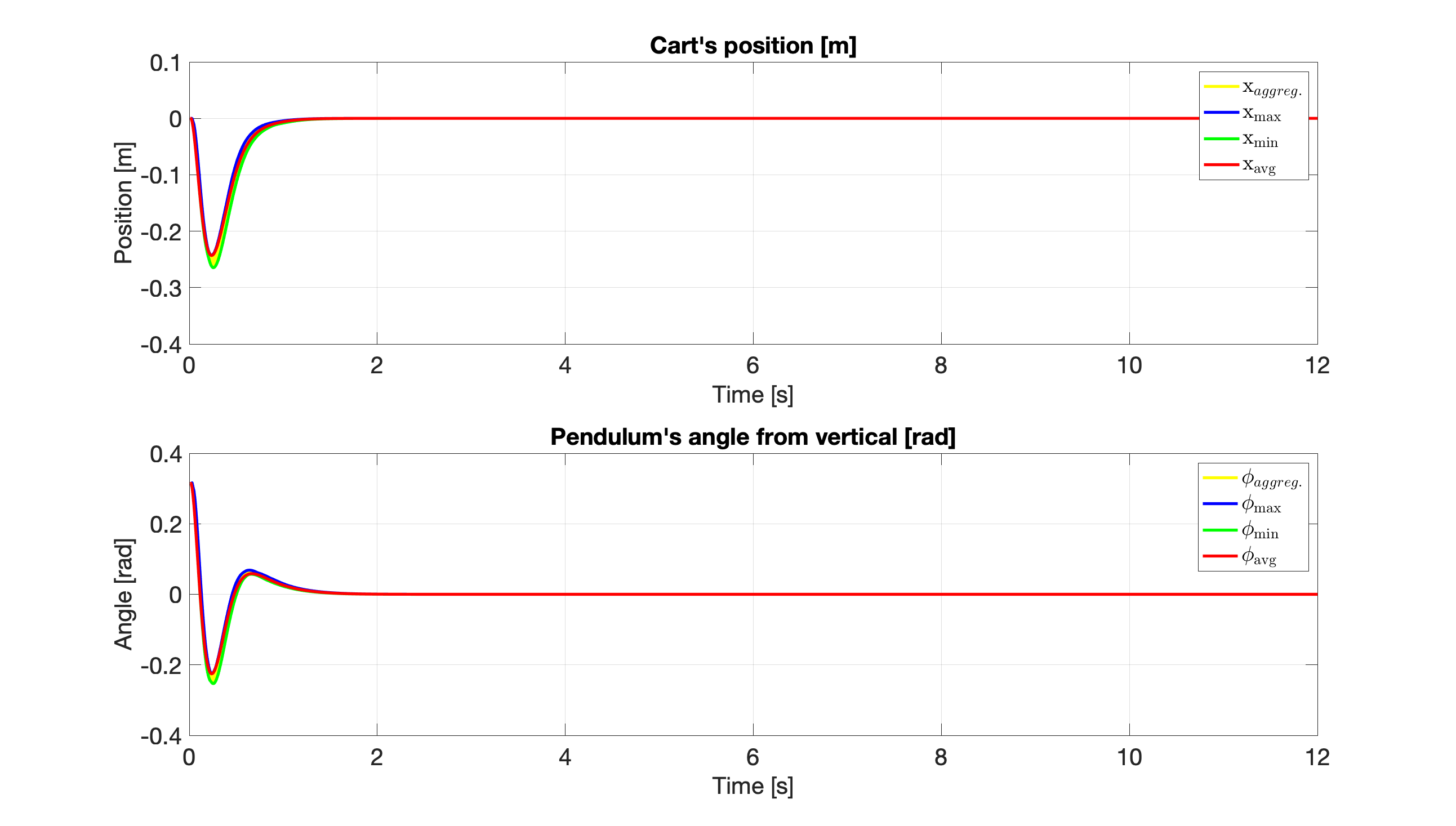
Figure 1: Traces of the system’s state that are generated under the Markovian control law over WirelessHART channel $\hat{\Gamma}$ having $\hat{d}_{i}\!=\!14\,$m.

Figure 2: Traces of the system’s state that are generated under the Bernoulli control law over WirelessHART channel $\hat{\Gamma}$ having $\hat{d}_{i}\!=\!14\,$m.

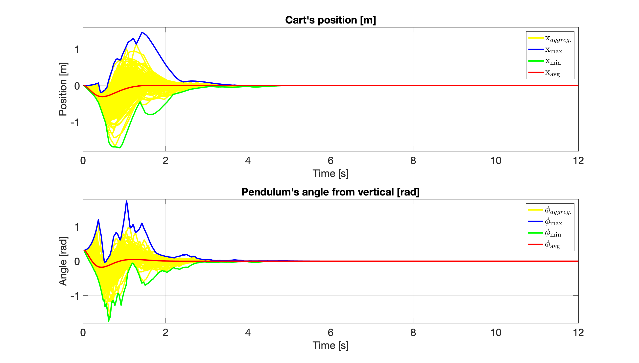
Figure 3: Traces of the system’s state that are generated under the Markovian control law over WirelessHART channel $\check{\Gamma}$ having $\check{d}_{i}\!=3.5\!\,$m.

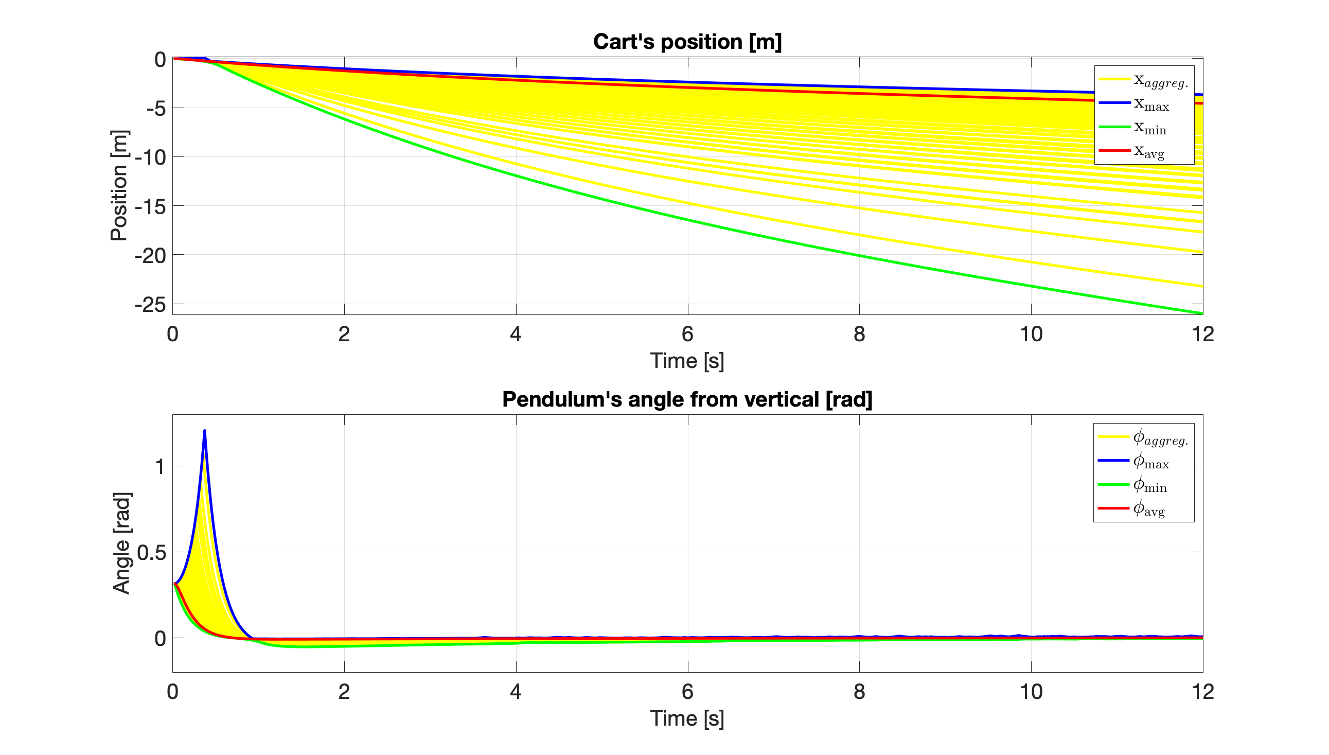
Figure 4: Traces of the system’s state that are generated under the Bernoulli control law over WirelessHART channel $\check{\Gamma}$ having $\check{d}_{i}\!=\!3.5\,$m.

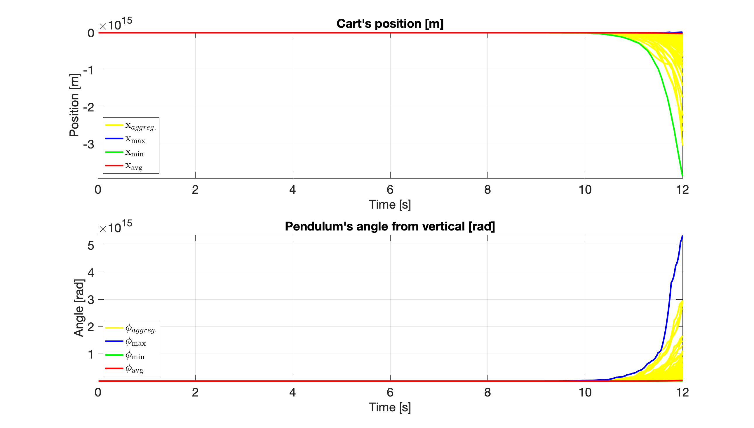
Figure 5: Traces of the system’s state that are generated under the Markovian control law over WirelessHART channel $\tilde{\Gamma}$ having $\tilde{d}_{i}\!=2.63\!\,$m.

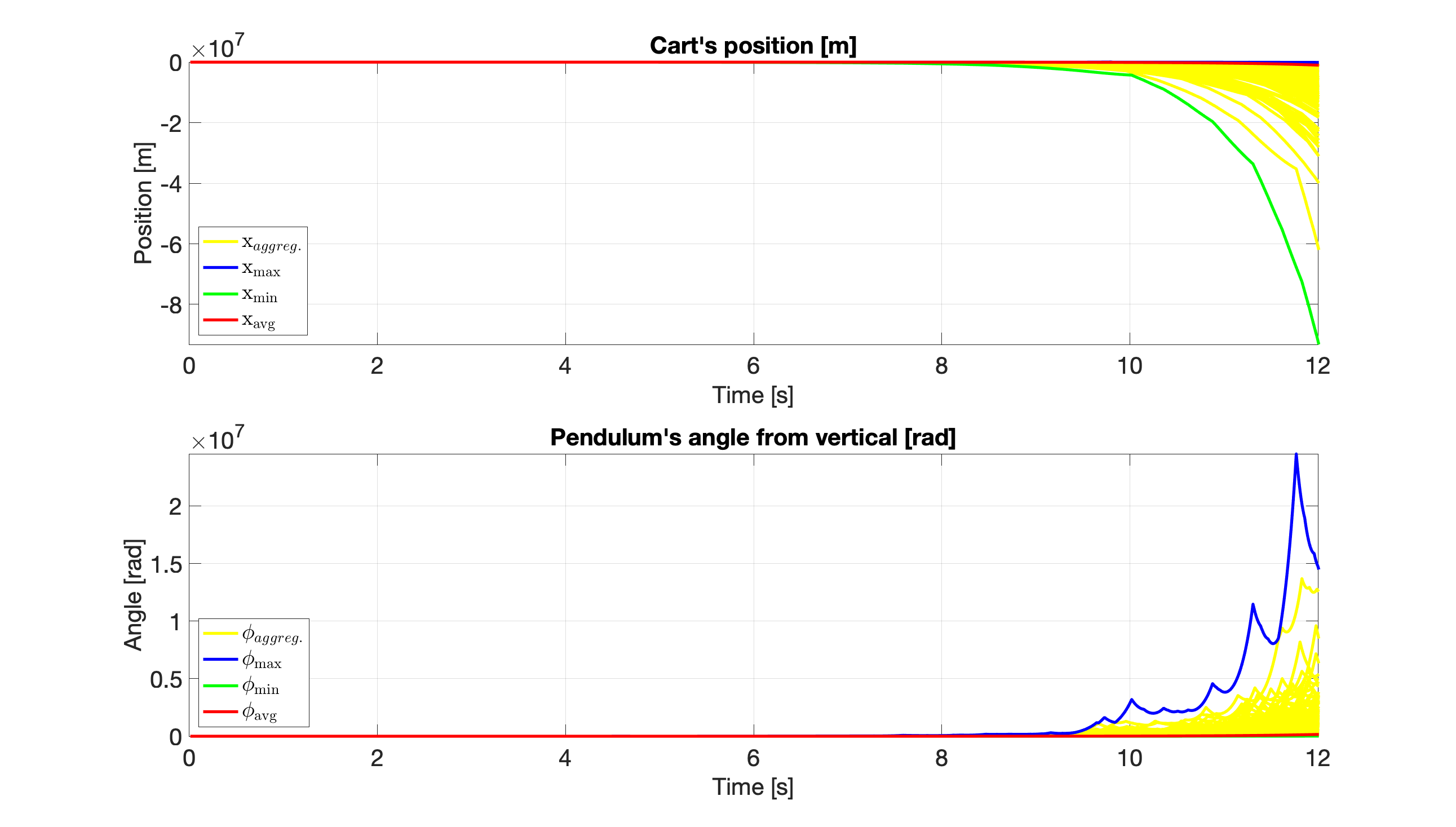
Figure 6: Traces of the system’s state that are generated under the Bernoulli control law over WirelessHART channel $\tilde{\Gamma}$ having $\tilde{d}_{i}\!=\!2.63\,$m.

APPENDIX

V-A Proof of Proposition 1

For (14), considering (3), (6) – (11), by the low of total probability, one has that

$$\mathrm{m}_{ij}^{(k+1)}\!\!\!=\!\mathbb{E}\!\left(\!x_{k+1}\mathbf{1}_{\left\{\theta_{k+1}=j,\,\theta_{k}=i\right\}}\!\right)\!\!=\!\!\left(\!\!A\!\!\sum\limits_{\ell=1}^{N}\!\!\!\mathrm{m}_{\ell i}^{(k)}\!\!\!+\!\!B\!\!\sum\limits_{\ell=1}^{N}\!\!K_{\ell}\mathrm{m}_{\ell i}^{(k)}\!\hat{\nu}_{i}\!\!\right)\!p_{ij}.$$

Similarly, for (1), by the low of total probability, considering again (3), (6) – (10), and (12), one has that

$$\mathrm{M}_{ij}^{(k+1)}\!=\!\mathbb{E}\!\left(x_{k+1}x_{k+1}^{*}\mathbf{1}_{\left\{\theta_{k+1}=j,\,\theta_{k}=i\right\}}\right)\!=$$

$$=\!\!\left(\!\!A\!\!\sum\limits_{\ell=1}^{N}\!\mathrm{M}_{\ell i}^{(k)}\!\!A^{*}\!\!\!+\!\!B\!\!\sum\limits_{\ell=1}^{N}\!\!K_{\ell}\mathrm{M}_{\ell i}^{(k)}\!K_{\ell}^{*}\!B^{*}\!\hat{\nu}_{i}\!+\!2\Re\!\!\left(\!\!A\!\!\sum\limits_{\ell=1}^{N}\!\!\mathrm{M}_{\ell i}^{(k)}\!K_{\ell}^{*}\!B^{*}\!\hat{\nu}_{i}\!\!\right)\!\!\!\right)\!p_{ij},$$

since from its definition (12), $\mathrm{M}_{\ell i}^{(k)}\!\succeq\!0$. ∎

V-B Proof of Proposition 2

We will follow the line of reasoning of the proof of a similar implication found in [9, Prop. 3.6, p. 35], which deals with classical MJLSs, having the operation modes observable instantaneously. Let $\left\{\tilde{e}_{i}\right\}_{i=1}^{n_{x}}$, $\left\{\hat{e}_{i}\right\}_{i=1}^{N^{2}n_{x}}$ and $\left\{\check{e}_{i}\right\}_{i=1}^{N^{2}n_{x}^{2}}$ be the canonical orthonormal basis for the linear spaces $\mathbb{F}^{n_{x}}$, $\mathbb{F}^{N^{2}n_{x}}$ and $\mathbb{F}^{N^{2}n_{x}^{2}}$, respectively. Fix arbitrarily $\zeta\!\in\!\left\{i\right\}_{i=1}^{n_{x}}$, $l\!\in\!\left\{i\right\}_{i=1}^{N}$, and $\iota\!\in\!\left\{i\right\}_{i=1}^{N}$. Consider the system (6), with the initial conditions $\theta_{-1}\!=\!l$, $\theta_{0}\!=\!\iota$, and $x_{0}\!=\!\tilde{e}_{\zeta}$. Then, the only element $\mathrm{m}_{\ell i}^{(0)}$ different from the vector of all zeros is $\mathrm{m}_{l\iota}^{(0)}\!=\!\tilde{e}_{\zeta}$, and $\mathrm{vec}^{2}\!\left({\mathbf{m}}^{(0)}\right)\!=\!\hat{e}_{\kappa}$, where $\kappa\!=\!\zeta\!+\!n_{x}\!\left(l\!-\!1\!+\!N\left(\iota\!-\!1\right)\!\right)$. Similarly, one has that the only element $\mathrm{M}_{\ell i}^{(0)}$ different from the null matrix is $\mathrm{M}_{l\iota}^{(0)}\!=\!\tilde{e}_{\zeta}\tilde{e}_{\zeta}^{*}$, and $\mathrm{vec}^{2}\!\left(\mathbf{M}^{(0)}\right)\!=\!\check{e}_{\varkappa}$, where $\varkappa\!=\!\zeta\!+\!n_{x}\!\left(\zeta\!-\!1\right)\!+\!n_{x}^{2}\!\left(l\!-\!1\!+\!N\left(\iota\!-\!1\right)\!\right)$. Now, on one hand one has from the repeated application of (19) that $\|\mathbf{m}^{(k)}\|_{\bm{2}}^{2}=\left\|{\bm{\Psi}}^{k}\hat{e}_{\kappa}\right\|_{2}^{2}$. On the other hand, from (11), by the triangle inequality, linearity of the expected value and of the trace, and by the definition of the trace, one has that

$$\left\|\mathbf{m}^{(k)}\right\|_{\bm{2}}^{2}\!\!=\!\!\sum\nolimits_{\ell=1}^{N}\!\sum\nolimits_{i=1}^{N}\!\left\|\mathrm{m}_{\ell i}^{(k)}\right\|_{2}^{2}\!\leq\!\sum\nolimits_{\ell=1}^{N}\!\sum\nolimits_{i=1}^{N}\left\|\mathrm{M}_{\ell i}^{(k)}\right\|_{\bm{1}}\!=\!\left\|{\bm{\Lambda}}^{\!k}\check{e}_{\varkappa}\right\|_{1}.$$

Now, the hypothesis $\rho\!\left({\bm{\Lambda}}\right)\!<\!1\!\Rightarrow\!\lim\nolimits_{k\to\infty}{\bm{\Lambda}}^{\!k}\!=\!0$. Thus, $\lim\nolimits_{k\to\infty}\left\|{\bm{\Psi}}^{k}\hat{e}_{\kappa}\right\|_{2}^{2}\!=\!0$. Since $\zeta$, $l$ and $\iota$ were chosen arbitrarily, it follows that the previous expression holds $\forall\kappa\!\in\!\left\{i\right\}_{i=1}^{N^{2}n_{x}}$. Hence, $\lim\nolimits_{k\to\infty}\left\|{\bm{\Psi}}^{k}{\bm{v}}\right\|_{2}^{2}\!=\!0$, $\forall{\bm{v}}\!\in\!\mathbb{F}^{N^{2}n_{x}}$, which implies that $\lim\nolimits_{k\to\infty}{\bm{\Psi}}^{k}\!=\!0$, and proves the thesis, $\rho\!\left({\bm{\Psi}}\right)\!<\!1$. ∎

V-C Proof of Proposition 3

For finite-dimensional linear spaces all norms are equivalent [11, Theorem 4.27], so one can choose any particular norm in (23). We first prove that $\rho\!\left({\bm{\Lambda}}\right)\!<\!1$ implies the mean square stability of the system (6). From the definition of the $\ell_{1}$ norm, triangle inequality and (13), one finds that

$$\left\|\mathbf{M}^{(k)}\right\|_{\bm{1}}\!\!\!=\!\!\sum\nolimits_{\ell=1}^{N}\!\sum\nolimits_{i=1}^{N}\!\left\|\mathrm{M}_{\ell i}^{(k)}\right\|_{\bm{1}}\!\!\geq\!\left\|\sum\nolimits_{\ell=1}^{N}\!\sum\nolimits_{i=1}^{N}\!\!\mathrm{M}_{\ell i}^{(k)}\right\|_{\bm{1}}\!\!\!=\!\left\|\mathbb{E}\!\left(x_{k}x_{k}^{*}\right)\right\|_{\bm{1}}\!\!.$$

By induction from (20) and the definition of the $\ell_{1}$ norm, $\|\mathbf{M}^{(k)}\|_{\bm{1}}=\|\mathrm{vec}^{2}\!(\!\mathbf{M}^{(k)}\!)\|_{1}=\|{\bm{\Lambda}}^{k}\mathrm{vec}^{2}\!(\!\mathbf{M}^{(0)}\!)\|_{1}$. Since $\rho\!\left({\bm{\Lambda}}\right)\!<\!1$ implies that $\lim\nolimits_{k\to\infty}{\bm{\Lambda}}^{\!k}\!=\!0$, so that $\lim\nolimits_{k\to\infty}\|\mathbf{M}^{(k)}\|_{\bm{1}}\!\!=\!0$, and, consequently, $\lim\nolimits_{k\to\infty}\left\|\mathbb{E}\left(x_{k}x_{k}^{*}\right)\!-\!0\right\|_{\bm{1}}\!\!=\!0$.

By following exactly the same line of reasoning, from Proposition 2, the definition of the $\ell_{1}$ norm, triangle inequality, (13), and the repeated application of (19), one finds that $\|\mathbf{m}^{(k)}\|_{\bm{1}}\!=\!\|\mathbb{E}(x_{k})\|_{1}$, $\|\mathbf{m}^{(k)}\|_{\bm{1}}\!=\!\|{\bm{\Psi}}^{k}\mathrm{vec}^{2}(\!\mathbf{m}^{(0)}\!)\|_{1}$ and $\rho({\bm{\Lambda}})\!<\!1\!\Rightarrow\!\lim\nolimits_{k\to\infty}\|\mathbb{E}(x_{k})\!-\!0\|_{1}\!\!=\!0$ $\forall x_{k}$, and the first part of the proof is concluded.

So, it remains to prove the sufficiency, i.e., the conditions in (23) imply that $\rho\!\left({\bm{\Lambda}}\right)\!<\!1$. By hypothesis, one has that $\lim\nolimits_{k\to\infty}\left\|\mathbb{E}\!\left(x_{k}x_{k}^{*}\right)\!-\!\mathrm{M}_{e}\right\|\!=\!0$ for all initial condition $\left(\hat{x}_{0},\theta_{0}\right)$. By taking $\hat{x}_{0}\!=\!0$, one finds that $\mathrm{M}_{e}$ must necessarily be equal to zero, and $\lim\nolimits_{k\to\infty}\mathbb{E}\!\left(x_{k}x_{k}^{*}\right)\!=\!0$. Then, from (13), it follows that $\lim\nolimits_{k\to\infty}\sum\nolimits_{\ell=1}^{N}\sum\nolimits_{i=1}^{N}\mathrm{M}_{\ell i}^{(k)}\!=\!0$, with $\mathrm{M}_{\ell i}^{(k)}\!\succeq\!0$, $\forall k,\ell,i$. Thus, from (12), one has that $\lim\nolimits_{k\to\infty}\mathbf{M}^{(k)}\!=\!0$. Since the linear mapping $\mathrm{vec}^{2}\!\left(\cdot\right)$ is uniform homeomorphic (see e.g. [13] for additional details), the convergent behaviour of $\mathbf{M}^{(k)}$ is preserved by $\mathrm{vec}^{2}\!\left(\!\mathbf{M}^{(k)}\!\right)$. So, from the repeated application of (20), one obtains that $\lim\nolimits_{k\to\infty}{\bm{\Lambda}}^{k}\mathrm{vec}^{2}\!\left(\!\mathbf{M}^{(0)}\!\right)\!=\!0$. This last statement is true $\forall\mathbf{M}^{(0)}$ if and only if (from now on, iff) $\lim\nolimits_{k\to\infty}{\bm{\Lambda}}^{k}\!=\!0$, i.e., iff $\rho\!\left({\bm{\Lambda}}\right)\!<\!1$. ∎

V-D Proof of Proposition 4

The proof of necessity follows the same steps of the proof of [9, Theorem 3.19, p. 41], if one considers the system described by the following recursive equation $\mathbf{T}^{(k+1)}\!=\!\mathcal{T}\!(\!\mathbf{T}^{(k)}\!)\!\!\;$, $\mathbf{T}^{(0)}\!\!\in\!\mathbb{F}^{Nn_{x}\times Nn_{x}}$, and $~{}\mathbf{T}^{(0)}\!\succ\!0$. An interested reader may also refer to [23, Lemmas 47, 54, pp. 214 – 216] for additional details on the proof for the simple linear case (without jumps). The proof of sufficiency instead is obtained by following the line of reasoning of the aforementioned [23, Lemma 54, pp. 215 – 216], and [24, Lemma 1]. ∎

V-E Proof of Proposition 5

By hypothesis on the process noise, $\forall k\!\in\!\mathbb{N}_{0}$, one has that $\mathbb{E}\!\left(w_{k}\right)\!=\!0$ and $\mathbb{E}\!\left(w_{k}w_{k}^{*}\right)\!=\!\Sigma_{w}$, and the first statement is obtained by the same line of reasoning of the first part of the proof of Proposition 1, after taking into account that $w_{k}$ is independent from $\theta_{k}$ and $\theta_{k-1}$.

The expression (5) is derived in similar fashion from the law of total probability, the aforementioned hypothesis, (3), (7) – (10), (12), and (22), observing that $\mathrm{M}_{\ell i}^{(k)}\!\succeq\!0$. ∎

V-F Proof of Theorem 1

We prove first that $\rho\!\left({\bm{\Lambda}}\right)\!<\!1$ implies that under the stated assumptions the system (22) is mean square stable.

Let $\mathbb{E}\!\left(\mathbf{1}_{\left\{\theta_{k}=i\right\}}\right)\!\triangleq\!\chi_{i}^{(k)}$ be the probability mass function of the MC $\Theta$. By the definition of the conditional probability, $\pi_{\ell i}^{(k)}\!=\!p_{\ell i}\chi_{\ell}^{(k-1)}$. So, $\chi_{i}^{(k)}\!=\!\sum\nolimits_{\ell=1}^{N}\pi_{\ell i}^{(k)}$. By hypothesis, $\Theta$ is ergodic, i.e., for any given initial probability distribution $\left\{\hat{\chi}_{i}^{(0)}\right\}_{i=1}^{\!N}$, there exists a limit probability distribution $\left\{\hat{\chi}_{i}^{(\infty)}\right\}_{i=1}^{\!N}$ which does not depend on $\left\{\hat{\chi}_{i}^{(0)}\right\}_{i=1}^{\!N}$, such that $\sum\nolimits_{i=1}^{N}p_{ij}\hat{\chi}_{i}^{(\infty)}\!=\!\hat{\chi}_{j}^{(\infty)}$, $\sum\nolimits_{i=1}^{N}\hat{\chi}_{i}^{(\infty)}\!=\!1$ and $|\chi_{i}^{(k)}\!-\hat{\chi}_{i}^{(\infty)}|\!\leq\!\eta\varepsilon^{k}$, for some $\eta\!\geq\!0$ and $0\!<\!\varepsilon\!<\!1$ (cf. [9, p. 48]). Let $\hat{\pi}_{\ell i}^{(\infty)}\!\!=\!p_{\ell i}\hat{\chi}_{\ell}^{(\infty)}\!$, $\hat{\bm{\Pi}}^{(\infty)}\!\!=\!\!\Big{[}\hat{\pi}_{\ell i}^{(\infty)}\!\!\otimes\!\mathbb{I}_{n_{x}}\Big{]}_{\ell,i=1}^{N}\!$. Then, from the ergodic assumption, $\sum\nolimits_{\ell=1}^{N}\hat{\pi}_{\ell i}^{(\infty)}\!=\!\hat{\chi}_{i}^{(\infty)}$, $\sum\nolimits_{\ell=1}^{N}\sum\nolimits_{i=1}^{N}\hat{\pi}_{\ell i}^{(\infty)}\!=\!1$, and, since by its definition $p_{\ell i}\!\geq\!0$, we have that $p_{\ell i}\left|\chi_{\ell}^{(k)}\!-\hat{\chi}_{\ell}^{(\infty)}\right|\!\leq\!p_{\ell i}\eta\varepsilon^{k}$,

$$\left|\pi_{\ell i}^{(k+1)}\!-\hat{\pi}_{\ell i}^{(\infty)}\right|\!\leq\!p_{\ell i}\eta\varepsilon^{k},~{}\eta\!\geq\!0,~{}0\!<\!\varepsilon\!<\!1.$$ (30)

We know from Proposition 5 that the first and the second moments of the system’s state evolve according to (19) and (27), respectively. By Proposition 2, $\rho\!\left({\bm{\Lambda}}\right)\!<\!1\!\Rightarrow\!\rho\!\left({\bm{\Psi}}\right)\!<\!1$. Thus, $\lim\limits_{k\to\infty}\!{\bm{\Psi}}^{k}\!\!=\!0$, and $\lim\limits_{k\to\infty}\left\|\mathbb{E}\left(x_{k}\right)\!-\!x_{e}\right\|\!=\!0$, where $x_{e}\!=\!0$, for all initial conditions $\left(\hat{x}_{0},\theta_{0}\right)$. Now, in order to show that also $\lim\limits_{k\to\infty}\left\|\mathbb{E}\left(x_{k}x_{k}^{*}\right)\!-\!{M}_{e}\right\|\!=\!0$, we will prove that $\left(\!\mathcal{Z}_{k}\right)_{k=0}^{\infty}$, with $\mathcal{Z}_{k}\!=\!{\bm{\Upsilon}}\mathrm{vec}^{2}\!\left(\!{\bm{\Pi}}^{(k)}\!\right)\!$, is a Cauchy summable sequence, i.e., it is a Cauchy sequence in a complete normed space $\mathbb{F}^{N^{2}n_{x}^{2}}$, and $\sum\limits_{k=0}^{\infty}\sup\limits_{\tau\geq 0}\left\|\mathcal{Z}_{k+\tau}\!-\!\mathcal{Z}_{k}\right\|\!<\!\infty$, so that $\mathrm{vec}^{2}\!\!\left(\!\mathbf{M}^{(k)}\!\right)$ from (27) is also Cauchy summable, and for any initial condition $\mathrm{vec}^{2}\!\!\left(\!\mathbf{M}^{(0)}\!\right)$, by [9, Proposition 2.9, p. 20] $\lim\limits_{k\to\infty}\mathrm{vec}^{2}\!\!\left(\!\mathbf{M}^{(k)}\!\right)\!=\!\left(\mathbb{I}_{N^{2}n_{x}^{2}}\!-\!{\bm{\Lambda}}\right)^{\!-1}\!{\bm{\Upsilon}}\!\lim\limits_{k\to\infty}\mathrm{vec}^{2}\!\left(\!{\bm{\Pi}}^{(k)}\!\right)$. Since for a finite-dimensional linear spaces all norms are equivalent, we will use $\ell_{1}$ norm to prove first that the elements of the sequence $\left(\mathcal{Z}_{k}\right)_{k=0}^{\infty}$ become arbitrarily close to each other as the sequence progresses, i.e., $\left(\mathcal{Z}_{k}\right)_{k=0}^{\infty}$ is a Cauchy sequence. Formally, $\forall t,k$, from the definition of the $\ell_{1}$-norm, triangle inequality, additivity of the linear mapping $\mathrm{vec}^{2}\!\left(\cdot\right)$, and (30)

$$\left\|\mathcal{Z}_{t}-\!\mathcal{Z}_{k}\right\|_{1}\!=\!\Big{\|}{\bm{\Upsilon}}\!\Big{(}\!\mathrm{vec}^{2}\!\Big{(}{\bm{\Pi}}^{(t)}\!\!-\!\hat{\bm{\Pi}}^{(\infty)}\!\Big{)}\!+\mathrm{vec}^{2}\!\Big{(}\hat{\bm{\Pi}}^{(\infty)}\!\!-\!{\bm{\Pi}}^{(k)}\!\Big{)}\!\!\Big{)}\!\Big{\|}_{1}\!\leq\!$$ (31)

$$\big{\|}{\bm{\Upsilon}}\big{\|}_{\bm{1}}\!\bigg{(}\!\Big{\|}{\bm{\Pi}}^{(t)}\!\!-\!\hat{\bm{\Pi}}^{(\infty)}\Big{\|}_{\bm{1}}\!\!\!+\!\Big{\|}\hat{\bm{\Pi}}^{(\infty)}\!\!-\!{\bm{\Pi}}^{(k)}\Big{\|}_{\bm{1}}\!\bigg{)}\!\leq\!N^{2}n_{x}\big{\|}{\bm{\Upsilon}}\big{\|}_{\bm{1}}\!\eta\!\left(\varepsilon^{t-1}\!\!+\!\varepsilon^{k-1}\right)\!,$$

for some $\eta\!\geq\!0$, $0<\!\varepsilon\!<\!1$, proving that $\left(\mathcal{Z}_{k}\right)_{k=0}^{\infty}$ is a Cauchy sequence, with $\!\lim\limits_{k\to\infty}\!\!\mathcal{Z}_{k}\!=\!{\bm{\Upsilon}}\mathrm{vec}\Big{(}\!\hat{\bm{\Pi}}^{(\infty)}\!\Big{)}\!$. Also, for $t\!=\!k\!+\!\tau$, (31) implies that $\sum\limits_{k=0}^{\infty}\sup\limits_{\tau\geq 0}\|\mathcal{Z}_{k+\tau}\!-\!\mathcal{Z}_{k}\|_{1}\!\leq\!\frac{2N^{2}n_{x}\eta}{\varepsilon(1\!-\!\varepsilon)}\big{\|}{\bm{\Upsilon}}\big{\|}_{\bm{1}}\!<\!\infty$. where the last equality is obtained from the formula of the sum of a geometric series. This proves that the sequence $\left(\mathcal{Z}_{k}\right)_{k=0}^{\infty}$ is Cauchy summable. Thus, by [9, Proposition 2.9, p. 20], if $\rho\!\left({\bm{\Lambda}}\right)\!<\!1$, then also $\mathrm{vec}^{2}\!\!\left(\!\mathbf{M}^{(k)}\!\right)$ from (27) is a Cauchy summable sequence, and for any initial condition $\mathrm{vec}^{2}(\mathbf{M}^{(0)})$, $\lim\limits_{k\to\infty}\mathrm{vec}^{2}(\mathbf{M}^{(k)})=(\mathbb{I}_{N^{2}n_{x}^{2}}-{\bm{\Lambda}})^{-1}{\bm{\Upsilon}}\mathrm{vec}^{2}\!\Big{(}\hat{\bm{\Pi}}^{(\infty)}\Big{)}$. Since $\mathrm{vec}^{2}\!\left(\cdot\right)$ is uniform homeomorphic, it follows that $\lim\limits_{k\to\infty}\!\mathbf{M}^{(k)}=\mathbf{M}^{(\infty)}$. Thus, together with (12) and (13), it implies that $\lim_{k\to\infty}\|\mathbb{E}(x_{k}x_{k}^{*})-\sum\limits_{\ell=1}^{N}\sum\limits_{i=1}^{N}\mathrm{M}_{\ell i}^{(\infty)}\|=0$. Hence, the system (22) is mean square stable. So, it remains to prove the necessity, i.e., if the system (22) is mean square stable, then $\rho\!\left({\bm{\Lambda}}\right)\!<\!1$. From (9), it is immediate to verify that

$$\mathrm{vec}^{2}\!\!\left(\!{\bm{\Pi}}^{(k)}\!\right)\!\!=\!{\bm{\Xi}}\,\mathrm{vec}^{2}\!\!\left(\!{\bm{\Pi}}^{(k-1)}\!\right)\!,\quad{\bm{\Xi}}\!=\!\Delta\mathrm{P}_{1}\!\otimes\!\!\left(\mathop{\mathchoice{\vbox{\hbox{\leavevmode\resizebox{8.25pt}{}{\rotatebox[origin={c}]{90.0}{$\displaystyle\bm{\ominus}$}}}}}{\vbox{\hbox{\leavevmode\resizebox{8.25pt}{}{\rotatebox[origin={c}]{90.0}{$\textstyle\bm{\ominus}$}}}}}{\vbox{\hbox{\leavevmode\resizebox{6.22499pt}{}{\rotatebox[origin={c}]{90.0}{$\scriptstyle\bm{\ominus}$}}}}}{\vbox{\hbox{\leavevmode\resizebox{4.875pt}{}{\rotatebox[origin={c}]{90.0}{$\scriptscriptstyle\bm{\ominus}$}}}}}}\slimits@\limits_{j=1}^{N}\mathbb{I}_{n_{x}^{2}}\!\right)\!,$$ (32)

and from (27) we have that

$$\mathrm{vec}^{2}\!\!\left(\!\mathbf{M}^{(k+1)}\!\right)\!=\!\bm{\Lambda}^{\!k}\mathrm{vec}^{2}\!\!\left(\!\mathbf{M}^{(0)}\!\right)\!+\!\!\sum\nolimits_{t=0}^{k-1}\!{\bm{\Lambda}}^{\!t}{\bm{\Upsilon}}{\bm{\Xi}}^{k-t-1}\mathrm{vec}^{2}\!\!\left(\!{\bm{\Pi}}^{(0)}\!\right)\!,$$ (33)

where, from (12), (IV), (28) and (32), only the first addend depends on the initial state $x_{0}$. By hypothesis the system is mean square stable, so, from (23) and (13), there exists $M_{e}$ (depending only on the process noise characteristics) such that $\lim\limits_{k\to\infty}\!\mathbb{E}\!\left(x_{k}x_{k}^{*}\right)\!=\!M_{e}$ for any $\mathbb{E}\!\left(x_{0}x_{0}^{*}\right)\!=\!\!\sum\nolimits_{\ell=1}^{N}\sum\nolimits_{i=1}^{N}\mathrm{M}_{\ell i}^{(0)}$. Since the linear mapping $\mathrm{vec}^{2}\!\left(\cdot\right)$ is uniform homeomorphic, (33) implies that $\mathbf{M}^{(k+1)}$ equals to

$$\mathrm{vec}^{-2}\!\!\left(\!\bm{\Lambda}^{\!k}\mathrm{vec}^{2}\!\left(\!\mathbf{M}^{(0)}\!\right)\!\!\right)\!\!+\!\!\!\sum\nolimits_{t=0}^{k-1}\!\mathrm{vec}^{-2}\!\!\left(\!{\bm{\Lambda}}^{\!t}{\bm{\Upsilon}}{\bm{\Xi}}^{k-t-1}\mathrm{vec}^{2}\!\!\left(\!{\bm{\Pi}}^{(0)}\!\right)\!\!\right)\!.\!\!$$ (34)

For $\hat{x}_{0}\!=\!0$, we have that the first addend in (34) produces a null matrix, while the second addend produces a matrix, denoted by ${\bm{W}}^{(k)}$, that is partitioned into the blocks of size $n_{x}$-by-$n_{x}$, such that ${\bm{W}}^{(k)}\!=\!\Big{[}W_{\ell i}^{(k)}\Big{]}_{\ell,i=1}^{N}$, and

$$\mathrm{M}_{e}\!=\!\lim\nolimits_{k\to\infty}\sum\nolimits_{\ell=1}^{N}\sum\nolimits_{i=1}^{N}W_{\ell i}^{(k)}\!.$$ (35)

Therefore, for any initial condition $\left(\hat{x}_{0},\hat{\varphi}_{0}\right)$, i.e., for any $\mathbf{M}^{(0)}$, by the definition of the matrix addition as entry-wise sum, it follows that $\lim\nolimits_{k\to\infty}\mathbb{E}(x_{k+1}x_{k+1}^{*})\!-\!M_{e}\!=\!0\!=\!\sum\nolimits_{\ell=1}^{N}\sum\nolimits_{i=1}^{N}(\mathrm{M}_{\ell i}^{(k+1)}\!-\!W_{\ell i}^{(k)})$, where $\mathrm{M}_{\ell i}^{(k)}\!\succeq\!0$, $\forall\ell,i,k$. This implies that $\forall\mathbf{M}^{(0)}$, $\lim\nolimits_{k\to\infty}\mathrm{vec}^{-2}(\bm{\Lambda}^{k}\mathrm{vec}^{2}(\mathbf{M}^{(0)}))\!=\!0$, which holds if and only $\lim\nolimits_{k\to\infty}\!\bm{\Lambda}^{\!k}\!=\!0$, and thus iff $\rho\!\left({\bm{\Lambda}}\right)\!<\!1$. ∎

V-G Proof of Theorem 2

$$\text{Define~{}}\mathbb{V}\!\triangleq\!\Big{\{}{\mathbf{V}_{{}_{\!1}}}\!=\!\big{[}V_{{{}_{\!1}}{\ell i}}\big{]}_{\ell,i=1}^{N},{\mathbf{V}_{{}_{\!2}}}\!=\!\big{[}V_{{{}_{\!2}}{\ell i}}\big{]}_{\ell,i=1}^{N},{\mathbf{V}_{{}_{\!3}}}\!=\!\big{[}V_{{{}_{\!3}}{\ell i}}\big{]}_{\ell,i=1}^{N},$$

$$\quad\mathbf{L}\!=\!\big{[}L_{i}\big{]}_{i=1}^{N}~{}\Big{|}~{}V_{{{}_{\!1}}{\ell i}}\!\in\!\mathbb{F}^{\,n_{x}\times n_{x}}\!,V_{{{}_{\!2}}{\ell i}}\!\in\!\mathbb{F}^{\,n_{x}\times n_{u}}\!,V_{{{}_{\!3}}{\ell i}}\!\in\!\mathbb{F}^{\,n_{u}\times n_{u}}\!,$$

$$\quad L_{i}\!\in\!\mathbb{F}^{n_{u}\times n_{x}}\!,V_{{{}_{\!1}}{\ell i}}\!\succ\!0,V_{{{}_{\!3}}{\ell i}}\!\succeq\!0,\text{\;satisfy\;}\eqref{eq:delayedStabilizabilityLMI}~{}\forall\ell,i\Big{\}}.$$

Since $V_{{{}_{\!1}}{ij}}\!\succ\!0$, (29a) is equivalent to $L_{i}V_{{{}_{\!2}}{ij}}\!\succeq\!V_{{{}_{\!2}}{ij}}^{*}V_{{{}_{\!1}}{ij}}^{-1}V_{{{}_{\!2}}{ij}}$ (by the Schur complement, see e.g. [9, Lemma 2.23, p. 28], [25, Section A.5.5, pp. 650 – 651]). To prove the necessity, we assume that the system (4) is mean square stabilizable. Then, by Definition 1, there is a mode-dependent state-feedback controller $\mathbf{K}\!=\!\left(K_{i}\right)_{i=1}^{N}$ such that the system (22), with $\mathfrak{A}_{\varphi_{k}}\!\triangleq\!A\!+\!\nu_{\theta_{k}}BK_{\theta_{k-1}}$, is mean square stable. Then, by Theorem 1, $\rho\!\left({\bm{\Lambda}}\right)\!\!<\!1$, and by Proposition 4, $\exists\mathbf{Y}\!=\!\!\left[\mathrm{Y}_{ij}\right]_{i,j=1}^{N}$, $\mathrm{Y}_{ij}\!\in\!\mathbb{F}^{n_{x}\times n_{x}}$, $\mathrm{Y}_{ij}\!\succ\!0$, such that $\mathrm{Y}_{ij}\!-\!\mathcal{L}_{ij}\!\left(\mathbf{Y}\right)\!\succ\!0,\forall i,j$, with $\mathcal{L}_{ij}\!\left(\mathbf{Y}\right)$ defined by (IV). After taking $V_{{{}_{\!1}}{ij}}\!=\!\mathrm{Y}_{ij}$, $V_{{{}_{\!2}}{ij}}\!=\!V_{{{}_{\!1}}{ij}}K_{i}^{*}$, $V_{{{}_{\!3}}{ij}}\!=\!V_{{{}_{\!2}}{ij}}^{*}V_{{{}_{\!1}}{ij}}^{-1}V_{{{}_{\!2}}{ij}}$, $L_{i}\!=\!K_{i}$, it is easy to verify from $\mathrm{Y}_{ij}\!-\!\mathcal{L}_{ij}\!\left(\mathbf{Y}\right)\!\succ\!0$ that (29) are satisfied and therefore the set $\mathbb{V}$ is not empty. To prove the sufficiency, we assume that $\mathbb{V}$ is non empty, so there are ${\mathbf{V}_{{}_{\!1}}},{\mathbf{V}_{{}_{\!2}}}$, ${\mathbf{V}_{{}_{\!3}}}$, and $\mathbf{L}$ that satisfy (29). Let $\mathbf{K}\!=\!\left(K_{i}\right)_{i=1}^{N}$, $K_{i}\!\in\!\mathbb{F}^{n_{u}\times n_{x}}$, be such that $V_{{{}_{\!2}}{ij}}\!=\!V_{{{}_{\!1}}{ij}}K_{i}^{*}$. By (29a), such $\mathbf{K}$ exists, and it may be obtained as $\mathbf{K}\!=\!\mathbf{L}$. Then, from (IV), (29), we have that $\mathcal{L}_{ij}\!\left({\mathbf{V}_{{}_{\!1}}}\!\right)\!-\!V_{{{}_{\!1}}{ij}}$ equals to

$$\!\Bigg{(}\!\!A\!\!\sum\nolimits_{\ell=1}^{N}\!\!\!\!V_{{{}_{\!1}}{\!\ell i}}A^{*}\!\!\!+\!\!B\!\!\sum\nolimits_{\ell=1}^{N}\!\!\!\!\!K_{\ell}\!V_{{{}_{\!1}}{\!\ell i}}K_{\ell}^{*}\!B^{*}\!\hat{\nu}_{i}\!\!+\!\!2\Re\!\Bigg{(}\!\!A\!\!\sum\nolimits_{\ell=1}^{N}\!\!\!V_{{{}_{\!1}}{\!\ell i}}K_{\ell}^{*}\!B^{*}\!\hat{\nu}_{i}\!\!\Bigg{)}\!\!\!\Bigg{)}p_{ij}\!\!-\!\!V_{{{}_{\!1}}{ij}}\!=$$

$$\sum\nolimits_{\ell=1}^{N}p_{ij}\!\left(AV_{{{}_{\!1}}{\!\ell i}}A^{*}\!\!\!+\!\!BV_{{{}_{\!3}}{\ell i}}B^{*}\!\hat{\nu}_{i}\!\!+\!\!AV_{{{}_{\!2}}{\ell i}}B^{*}\!\hat{\nu}_{i}\!\!+\!\!BV_{{{}_{\!2}}{\ell i}}^{*}A^{*}\!\hat{\nu}_{i}\right)\!-\!V_{{{}_{\!1}}{ij}}\!\prec\!0.$$

So, by Proposition 4, we have that $\rho\!\left({\bm{\Lambda}}\right)\!<\!1$, and thus, by Theorem 1, the system (22) is mean square stable. Then, by Definition 1, the system (4) is mean square stabilizable, and the proof is concluded. ∎

V-H Proof of Theorem 3

By hypothesis, $\left(\mathbf{p}_{i}\right)_{i=1}^{N}$ is the stationary distribution of the channel states, and $\hat{\nu}\!=\!\sum_{j=1}^{N}\mathbf{p}_{j}\hat{\nu}_{j}$. By definition of the steady state distribution, $\sum_{i=1}^{N}\mathbf{p}_{i}\!=\!1$, and $\mathbf{p}_{j}\!=\!\sum_{i=1}^{N}\mathbf{p}_{i}p_{ij}$, so $\hat{\nu}\!=\!\sum_{i=1}^{N}\mathbf{p}_{i}\sum_{j=1}^{N}p_{ij}\hat{\nu}_{j}$. Thus, the MARE can be written as $\sum_{i=1}^{N}\mathbf{p}_{i}\Big{(}X_{\infty}^{b}-\!A^{*}X_{\infty}^{b}A-Q\,+\sum_{j=1}^{N}p_{ij}\hat{\nu}_{j}\big{(}A^{*}X_{\infty}^{b}B\big{)}\!\big{(}R\!+\!B^{*}X_{\infty}^{b}B\big{)}^{{-1}}\!\big{(}B^{*}X_{\infty}^{b}A\big{)}\!\Big{)}\!=\!0$, holding $\forall\left(\mathbf{p}_{i}\right)_{i=1}^{N}$ iff, $\forall i\!\leq\!N$ the following expression is satisfied:

$$X_{\infty}^{b}=A^{*}X_{\infty}^{b}A+Q-\!\left(\sum\nolimits_{j=1}^{N}p_{ij}\hat{\nu}_{j}\!\right)\!Y,$$ (36)

where $Y\!\triangleq\!\big{(}A^{*}X_{\infty}^{b}B\big{)}\!\big{(}R\!+\!B^{*}X_{\infty}^{b}B\big{)}^{{-1}}\!\big{(}B^{*}X_{\infty}^{b}A\big{)}\!$. Since $p_{ij}$ and $\hat{\nu}_{j}$ are known scalars, $\sum\nolimits_{j=1}^{N}p_{ij}\hat{\nu}_{j}\!\triangleq\!\xi_{i}$, with $\xi_{i}$ again a known scalar. So, we focus on the term $\xi_{i}Y$. From the property of the product of invertible matrix with a non-zero scalar, it follows that $\xi_{i}Y\!=\!\big{(}\xi_{i}A^{*}X_{\infty}^{b}B\big{)}\!\big{(}\xi_{i}(R\!+\!B^{*}X_{\infty}^{b}B)\big{)}^{{-1}}\!\big{(}\xi_{i}B^{*}X_{\infty}^{b}A\big{)}$. Thus, we apply the definition of $\xi_{i}$ and substitute the last expression of $\xi_{i}Y$ in (36), obtaining exactly (5), where, as required by the mode-independence, $X_{\infty,i}^{c}\!=\!X_{\infty}^{b}$, $\forall i\!\leq\!N$. ∎

References

- [1] J. P. Hespanha, P. Naghshtabrizi, and Y. Xu, “A survey of recent results in networked control systems,” Proc. IEEE, vol. 95, no. 1, pp. 138–162, 2007.
- [2] W. M. H. Heemels, A. R. Teel, N. van de Wouw, and D. Nesic, “Networked control systems with communication constraints: Tradeoffs between transmission intervals, delays and performance,” IEEE Trans. Autom. Control, vol. 55, no. 8, pp. 1781–1796, 2010.
- [3] L. Schenato, B. Sinopoli, M. Franceschetti, K. Poolla, and S. S. Sastry, “Foundations of control and estimation over lossy networks,” Proc. IEEE, vol. 95, no. 1, pp. 163–187, 2007.
- [4] V. Gupta, A. F. Dana, J. P. Hespanha, R. M. Murray, and B. Hassibi, “Data transmission over networks for estimation and control,” IEEE Trans. Autom. Control, vol. 54, no. 8, pp. 1807–1819, 2009.
- [5] M. Pajic, S. Sundaram, G. J. Pappas, and R. Mangharam, “The wireless control network: a new approach for control over networks,” IEEE Trans. Autom. Control, vol. 56, no. 10, pp. 2305–2318, 2011.
- [6] P. Sadeghi, R. A. Kennedy, P. B. Rapajic, and R. Shams, “Finite-state Markov modeling of fading channels – a survey of principles and applications,” IEEE Signal Process. Mag., vol. 25, no. 5, pp. 57–80, 2008.
- [7] A. P. Gonçalves, A. R. Fioravanti, and J. C. Geromel, “Markov jump linear systems and filtering through network transmitted measurements,” Signal Process., vol. 90, no. 10, pp. 2842–2850, 2010.
- [8] I. Matei, N. C. Martins, and J. S. Baras, “Optimal linear quadratic regulator for Markovian jump linear systems, in the presence of one time-step delayed mode observations,” IFAC Proc., vol. 41, no. 2, pp. 8056–8061, 2008, 17th IFAC World Congr.
- [9] O. L. V. Costa, M. D. Fragoso, and R. P. Marques, Discrete-time Markov jump linear systems. Springer, 2005.
- [10] R. E. Megginson, An Introduction to Banach Space Theory, ser. Graduate Texts in Mathematics. Springer, 1998, vol. 183.
- [11] C. S. Kubrusly, Elements of operator theory. Birkhäuser, 2001.
- [12] R. A. Horn and C. R. Johnson, Matrix analysis, 2nd ed. CUP, 2012.
- [13] A. W. Naylor and G. R. Sell, Linear operator theory in engineering and science, ser. Appl. Math. Sci. Springer, 2000, vol. 40.
- [14] J. W. Brewer, “Kronecker products and matrix calculus in system theory,” IEEE Trans. Circuits Syst., vol. 25, no. 9, pp. 772–781, 1978.
- [15] BSI Standards Publication BS EN 62591:2016, Industrial communication networks – Wireless communication network and communication profiles – WirelessHART™, it is identical to IEC 62591:2016.
- [16] IEEE Std 802.15.4™-2006, Standard for Information technology – Local and metropolitan area networks – Specific requirements – Part 15.4: Wireless MAC and PHY Specifications for Low-Rate WPANs.
- [17] C. Fischione, F. Graziosi, and F. Santucci, “Approximation for a sum of On-Off log-normal processes with wireless applications,” IEEE Trans. Commun., vol. 55, no. 9, pp. 1822–1822, Sept 2007.
- [18] F. Barac, M. Gidlund, and T. Zhang, “Scrutinizing bit-and symbol-errors of IEEE 802.15.4 communication in industrial environments,” IEEE Trans. Instrum. Meas., vol. 63, no. 7, pp. 1783–1794, 2014.
- [19] J. G. Ruiz, B. Soret, M. C. Aguayo-Torres, and J. T. Entrambasaguas, “On finite state Markov chains for Rayleigh channel modeling,” in Wireless Commun., Veh. Technol., Inf. Theory Aerosp. Electron. Syst. Technol. (Wireless VITAE). IEEE, 2009, pp. 191–195.
- [20] M. Z. Chen, L. Zhang, H. Su, and G. Chen, “Stabilizing solution and parameter dependence of modified algebraic Riccati equation with application to discrete-time network synchronization,” IEEE Trans. Autom. Control, vol. 61, no. 1, pp. 228–233, Jan 2016.
- [21] S.-J. Wu and M. T. Chu, “Markov chains with memory, tensor formulation, and the dynamics of power iteration,” Appl. Math. Comput., vol. 303, pp. 226–239, 2017.
- [22] G. F. Franklin, J. D. Powell, and A. Emami-Naeini, Feedback control of dynamic systems, 6th ed. Prentice Hall, 2009.
- [23] F. M. Callier and C. A. Desoer, Linear system theory. Springer, 1991.
- [24] C. Kubrusly and O. Costa, “Mean square stability conditions for discrete stochastic bilinear systems,” IEEE Trans. Autom. Control, vol. 30, no. 11, pp. 1082–1087, 1985.
- [25] S. Boyd and L. Vandenberghe, Convex optimization. CUP, 2004.