Lotka–Volterra Competition Mechanism Embedded in a Decision-Making Method

Abstract

Decision making is a fundamental capability of living organisms, and has recently been gaining increasing importance in many engineering applications. Here, we consider a simple decision-making principle to identify an optimal choice in multi-armed bandit (MAB) problems, which is fundamental in the context of reinforcement learning. We demonstrate that the identification mechanism of the method is well described by using a competitive ecosystem model, i.e., the competitive Lotka–Volterra (LV) model. Based on the “winner-take-all” mechanism in the competitive LV model, we demonstrate that non-best choices are eliminated and only the best choice survives; the failure of the non-best choices exponentially decreases while repeating the choice trials. Furthermore, we apply a mean-field approximation to the proposed decision-making method and show that the method has an excellent scalability of $O(\log N)$ with respect to the number of choices $N$. These results allow for a new perspective on optimal search capabilities in competitive systems.

I Introduction

Recent research suggests that nature is a great source of inspiration in providing solutions for complicated problems and developing intelligent information processing Agarwal2014naturalComputing . Inspired by biological functions, physical structures, and organizational principles found in nature, numerous mathematical and metaheuristic models have been developed. These include genetic algorithms, ant colony optimization, bee algorithms, and simulated annealing, which have been used for addressing various optimization problems Agarwal2014naturalComputing ; Holland1989GA ; Dorigo1996AntColony ; Karaboga2007BeeAlgorithm ; Karaboga2008BeeAlgorithm ; Kirkpatrick1983SimulatedAnnealing ; Cerny1985SimulatedAnnealing .

Nature-inspired algorithms have also been applied to solve the multi-armed bandit (MAB) problem, which is fundamental in the context of decision making and reinforcement learning Sutton2018ReinforcementLearning . A major goal of the MAB problem is to identify the best choice (best arm) from the available options, i.e., best arm identification Audibert2010BestArmMAB . For this purpose, various methods have been developed Sutton2018ReinforcementLearning ; Audibert2010BestArmMAB ; Kim2010TOW ; Kim2015TOW in the face of a common difficulty; sufficient exploratory actions may allow us to determine the best choice with a high confidence level, but it may be accompanied by a cost. Among the methods, the one mentioned in the Refs. Kim2010TOW ; Kim2015TOW is based on an inspiration from the spatiotemporal dynamics of micro-organisms, such as amoebas, for identifying the best choice in an MAB problem. The dynamic stretching and contracting of amoebas when seeking food while maintaining their volume constant generates a frustrating non-local correlation as a whole, leading to an efficient and adaptive ability of identifying the best choice. At present, the amoeba-inspired decision-making method has been implemented in various physical systems Kim2010TOW ; Kim2015TOW ; Naruse2015SinglePhotonDM ; Kim2016harnessDM ; Naruse2017Ultrafast-photo ; Homma2019DecisionMaking ; however, the theoretical guarantee of the best choice identification has not yet been provided.

Meanwhile, a frustration similar to that in the amoeba dynamics, i.e., fluctuating dynamics under a conservative constraint, can generally be seen in a variety of competitive dynamical systems, in which each component (or state) competes for common finite resources. For instance, each species in an ecosystem attempts to grow its population while competing for limited resources. Such interspecific competition has been modeled by simple ordinary differential equations, known as the competitive Lotka–Volterra (LV) equations Baigent2016Lotka-Volterra ; Zeeman1995extinction . The LV equations describe the dynamics of competitive systems, such as multi-mode lasers Sargent1974LaserPhysics ; Sargent1993MultiModeLaser , as well as ecological communities Baigent2016Lotka-Volterra . Moreover, the LV model is closely related to the Moran process in the context of population genetics Noble2011LV-dynamics and evolutionary game theory Hofbauer2003Evolutionary , suggesting the applicability of the competitive mechanism to explore an optimal solution adapted to a given environment.

In this study, we propose a decision-making principle in which the LV competitive mechanism is embedded. The model is a natural and simple extension of the amoeba-inspired decision-making method Kim2010TOW ; Kim2015TOW and enables the identification of the best choice in the MAB problems, based on the competitive growth under a conservation law. We theoretically ensure the validity of the best choice identification, based on the LV competition model.

II Model

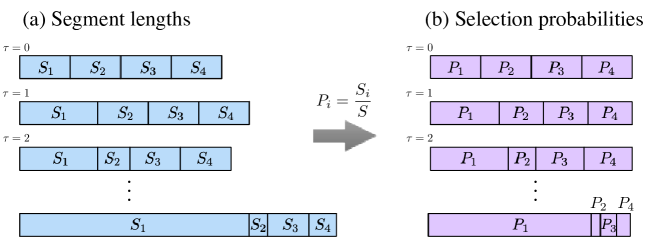
Figure 1: (Color online) Schematics of decision-making method. (a) Lengths of the object and each segment $S_{i}$ change according to Eq. (2). (b) Selection probabilities $P_{i}$ change according to the change in the segment lengths.

First, let us consider an MAB with $N$ arms providing unknown stochastic rewards $x_{1},\cdots,x_{N}$, where $x_{i}$ ($i=1,\cdots,N$) is assumed to be an independent realization of a random variable with mean $\mu_{i}$. The mean of the reward from the $i$-th arm is expressed as $\mu_{i}=\int\phi_{i}(x_{i})x_{i}\text{d}{x_{i}}$, where $\phi_{i}$ is the probability density of $x_{i}$. Without loss of generality, we assume that $\mu_{i}$ is positive. A goal of the MAB problem is to identify the best arm with the largest mean reward, $\mu_{i^{*}}=\max_{i}\{\mu_{i}\}$, through multiple plays, where $i^{*}$ is the best arm. Hence, the MAB problem can be considered, for example, as a decision-making problem for a gambler who plays slot machines (or a slot machine with multiple arms).

Our decision-making method for identifying the best arm is based on the dynamic behavior of an object with a total length of $S$, which consists of $N$ segments, as schematically shown in Fig. 1(a). Let $S_{i}(\tau)$ be the length of the $i$-th segment at the $\tau$-th play. At $\tau=0$, the length of each segment is assumed to be identical, e.g., $S_{i}(0)=1$. To identify the best arm, we repeat the following three processes:

(i) Selecting an arm to play: Select an arm with the following probability defined by the ratio of each segment length and total length $S(\tau)=\sum_{i=1}^{N}S_{i}(\tau)$ at the $\tau$-th play;

$$P_{i}(\tau)=S_{i}(\tau)/S(\tau)\quad\quad(i=1,2,...,N).$$ (1)

We refer to $P_{i}(\tau)$ as the selection probability of arm $i$ at the $\tau$-th play.

(ii) Playing the chosen arm: By playing the arm $i$ chosen in step (i), reward $x_{i}$ at the $\tau$-th play is received based on the reward probability distribution.

(iii) Learning and updating: The length of the $i$-th segment is altered based on the total length of the object and $x_{i}$:

$$S_{i}(\tau+1)=S_{i}(\tau)+b_{i}(x_{i},b)S(\tau),$$ (2)

where $b_{i}(x_{i},b)$ is a function of the reward $x_{i}$, and $b$ is a small incremental parameter. If $b_{i}(x_{i},b)<0$ and $S_{i}(\tau+1)<0$, $S_{i}(\tau+1)=0$ is set. Although one can choose an arbitrary form of the function $b_{i}(x_{i},b)$, we use the following function in this study:

$$b_{i}(x_{i},b)=\dfrac{b\ x_{i}}{1-b\ x_{i}},$$ (3)

where $0<b\ll 1$ is assumed such that $bx_{i}<1$. As the aforementioned processes (i)–(iii) are repeated, the length of each segment, $S_{i}(\tau)$, increases or decreases in accordance with the received reward [Fig. 1(a)]. As a result, the selection probability of the best arm $i^{*}$ with the largest mean reward, $P_{i^{*}}(\tau)=S_{i^{*}}(\tau)/S(\tau)$, increases compared to those of the others [Fig. 1(b)].

From Eqs. (1) and (2), the update of $P_{i}(\tau)$ is expressed as follows:

$$P_{i}(\tau+1)=P_{i}(\tau)+\Delta P_{i}(\tau),$$ (4)

$$\Delta P_{i}(\tau)=\begin{cases}\dfrac{b_{i}(x_{i},b)\left(1-P_{i}\right)}{1+b_{i}(x_{i},b)}=bx_{i}(1-P_{i}),\ \mbox{if arm $i$ is played,}\\ -\dfrac{b_{j}(x_{j},b)}{1+b_{j}(x_{j},b)}P_{i}=-bx_{j}P_{i},\ \mbox{if arm $j$ $(\neq i)$ is played,}\end{cases}$$ (5)

where Eq. (3) was used to derive $\Delta P_{i}(\tau)$.

The proposed decision-making method is analogous to ideal gases bounded by movable partitions in a vessel. That is, $P_{i}$ corresponds to the volume of the $i$-th gas bounded by the $(i-1)$-th and the $i$-th partitions, and the change in the volume of the $i$-th gas results from the increase or decrease in the number of moles of the $i$-th gas corresponding to $S_{i}$ [Fig. 1(b)].

The aforementioned method can also be regarded as a modified version of the tug-of-war model Kim2010TOW ; Kim2015TOW in the sense that the volume of each segment (probability $P_{i}$) grows and shrinks under the conservative condition of the total volume of the body ($\sum_{i}P_{i}=1$). Notably, the proposed decision-making method has a similarity to the linear reward schemes, known as classical schemes in learning automata Baba1985NewTopicsLA ; Narendra2015reviewLA , in the case of a binary bandit problem, as well as replicator equations in the field of evolutionary game theory Hofbauer2003Evolutionary .

As described in the next section, the LV competing principle is embedded in the proposed decision-making method; therefore, an exponential decrease in the error probability (the probability of choosing a non-best arm) is ensured.

III Results and Discussions

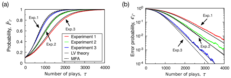
Figure 2: (Color online) Performance evaluation for three 10-armed bandit problems. $\tau$-dependences of (a) the mean selection probability of the best arm, $\bar{P}_{i^{*}}(\tau)$, and (b) the error probabilities in experiments 1, 2, and 3, which are indicated in red, green, and blue, respectively. These results were calculated based on the update rule (i)–(iii) explained in Sec. 2. The reward of each arm is assumed to be provided based on a normal distribution with mean $\mu_{i}$ $(i=1,2,\cdots,N)$ and variance $1/4$. In each experiment, $\mu_{i}$ was set as follows: Experiment 1: $\mu_{1}=0.4$ and $\mu_{2\leq i\leq 10}=0.2$. Experiment 2: $\mu_{1}=0.4$ and $\mu_{2\leq i\leq 10}$ were determined from uniform random distribution in the range from $0.1$ to $0.2$. Experiment 3: $\mu_{1}=0.6$, $\mu_{2\leq i\leq 5}=0.3$, and $\mu_{6\leq i\leq 10}=0.2$. The black solid curves in (a) and (b) were obtained by numerical integration of the competitive LV equation [Eq. (8)], and the black dashed curves are analytical solutions [Eqs. (14) and (15)] obtained by the mean-field approximation [see text].

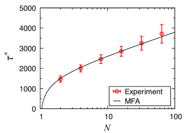
Figure 3: Average number of plays $\tau^{*}$ required for the error probability to satisfy $e_{i^{*}}(\tau)<\delta=0.05$ at $N$-armed bandit problems, where $b=0.005$, $\mu_{1}=0.6$, and $\mu_{2\leq i\leq N}=0.2$. The black solid curve is the theoretical estimation obtained by the mean-field approximation (MFA) for the competitive LV equation [see text and Eq. (16)].

Before revealing the connection between the proposed decision-making method and the LV competitive dynamics, we show the results of numerical simulations for three typical examples to demonstrate that our method typically has the ability to identify the best arm among multiple arms with unknown rewards. For the numerical demonstration, we set the number of arms $N=10$ and assumed that the reward of $i$-th arm, $x_{i}$, is provided based on a normal distribution, which is given by $\phi_{i}(x)=1/\sqrt{2\pi\sigma_{i}^{2}}\exp[-(x-\mu_{i})^{2}/(2\sigma_{i}^{2})]$, with the mean $\mu_{i}$ and variance $\sigma_{i}^{2}=1/4$ ($i=1,2,\cdots,10$). The best arm $i^{*}$ with the largest mean reward is set to be arm $1$, i.e., $\mu_{1}=\mu_{i^{*}}=\max_{i}\{\mu_{i}\}$. To quantify the capability of the best arm identification, consecutive arm playing was conducted until the cycle $\tau=4000$ (this makes up one “run”). Independently repeating this for $n_{s}=100$ runs, the mean of the selection probability of the best arm, $\bar{P}_{i^{*}}(\tau)=({1}/{n_{s}})\sum_{n=1}^{n_{s}}P^{(n)}_{i^{*}}(\tau)$, was evaluated, where $P^{(n)}_{i^{*}}(\tau)$ is the selection probability of the best arm at the $\tau$-th play of the $n$-th run.

Figure 2(a) shows the mean selection probability of the best arm as a function of $\tau$, $\bar{P}_{i^{*}}(\tau)$, which were calculated by the update rule (i)–(iii) in Sec. 2. As shown in this figure, $\bar{P}_{i^{*}}(\tau)$ in the three typical MAB problems depicted by red, green, and blue lines converges toward 1. Figure 2(b) shows that the error probability, $e_{i^{*}}(\tau)=1-\bar{P}_{i^{*}}(\tau)$, i.e., the probability of selecting the non-best arm, exponentially decreases. Hence, it is numerically shown that the proposed decision-making method works well in identifying the best arm (more rigid proof of the ability of the best arm identification will be provided in subsection III.2).

The selection probability of the best arm is expected to depend on $N$ as well as the difference between the mean rewards. The average number of plays $\tau^{*}$ resulting in the decision error probability being sufficiently small, i.e., $e_{i^{*}}(\tau)<\delta=0.05$, is demonstrated in Fig. 3 as a function of $N$. The figure clearly shows that the average number of plays $\tau^{*}$ increases only with $\log N$. The dependence of $O(\log N)$ will be important in the scalable solution of MAB problems with a large number of arms, and it is better than the Upper Confidence Bound Exploration (UCB-E) Audibert2010BestArmMAB and an extended tug-of-war model with $O(N)$-scalability Naruse2018Scalable-photon .

III.1 Hidden Lotka–Volterra Competition Dynamics

In this subsection, we show that the Lotka–Volterra type of interspecific competition dynamics lies behind our model and yields the performance of the decision-making method illustrated in the previous subsection.

The starting point of our analysis is Eq. (4) of the selection probability of each arm. We here consider the ensemble average of the selection probability of each arm at the $\tau$-th play; $\bar{P}_{i}(\tau)=(1/n_{s})\sum_{n=1}^{n_{s}}P_{i}^{(n)}(\tau)$, where $P_{i}^{(n)}(\tau)$ is the selection probability at the $\tau$-th play on the $n$-th run. The update of the ensemble average $\bar{P}_{i}(\tau)$ is described as follows:

$$\bar{P}_{i}(\tau+1)=\bar{P}_{i}(\tau)+\langle\Delta P_{i}(\tau)\rangle,$$ (6)

where $\left<\Delta P_{i}(\tau)\right>$ is the ensemble average of $\Delta P_{i}(\tau)$ for $n_{s}$ runs and is given by

$$\langle\Delta P_{i}(\tau)\rangle =b\bar{P}_{i}(\tau)\left(\mu_{i}-\sum_{j=1}^{N}\mu_{j}\bar{P}_{j}(\tau)\right).$$ (7)

The detailed derivation is described in Appendix A.

Next, we reconfigure “time” as $t\equiv\Delta t\tau=b\tau$. When $b$ is sufficiently small, $\mbox{$\bar{P}$}_{i}(t+\Delta t)=\mbox{$\bar{P}$}_{i}(t)+({\text{d}\mbox{$\bar{P}$}_{i}}/{\text{d}t})\Delta t+O\left(\Delta t^{2}\right)$; thus, the average dynamics of the selection probabilities are described as follows:

$$\frac{\text{d}\bar{P}_{i}}{\text{d}t}=\bar{P_{i}}\left(\mu_{i}-\sum_{j}\mu_{j}\bar{P}_{j}\right).$$ (8)

Note that Eq. (8) is equivalent to the competitive Lotka–Volterra (LV) equation, which describes competition among species competing for a common resource, as followsBaigent2016Lotka-Volterra :

$$\frac{\text{d}z_{i}}{\text{d}t}=z_{i}\left(a_{i}-\sum_{j=1}^{N}c_{ij}z_{j}\right),$$ (9)

where $z_{i}$ and $a_{i}$ represent the population of the species $i$ and the growth rate of the species $i$, respectively, and $c_{ij}$ represents intraspecific ($i=j$) and interspecific $(i\neq j)$ interactions. By comparing Eq. (8) to Eq. (9), searching for the best arm in our method can be interpreted as follows: $P_{i}$ attempts to “grow” according to $\mu_{i}$ (the mean reward of the arm $i$); however, the selection probabilities of the other arms also attempt to grow; thus, they compete for survival. The arm (species) that survives this competition will be considered the best arm. The origin of this competition mechanism lies in frustration, such as an ecosystem competing for limited resources, in which $P_{i}$ increases under the conservation conditions of total probability; $\sum_{i}P_{i}=1$.

As an example of such competition among arms, Fig. 4 shows the simulation results of the selection probability of each arm for 4-armed bandit problems, where $\mu_{1}$, $\mu_{2}$, $\mu_{3}$, and $\mu_{4}$ are given by $0.6$, $0.5$, $0.4$, and $0.3$, respectively. As a result of the competition among the arms, the selection probability of arm $1$ overwhelms those of the others. The numerical results agree well with the black solid curves shown in Fig. 4, which were obtained by numerical integration of Eq. (8) using the Euler method with time step $\Delta t=b$.

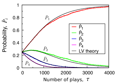
Figure 4: (Color online) $\tau$-dependence of the selection probability of arm $i$ in the 4-armed bandit problem with $\mu_{i}=0.6-(i-1)/10$  $(i=1,2,3,4)$. The black solid curves represent the results of the numerical integration of Eq. (8). Via the competition, arms 2, 3, and 4 are defeated in increasing order of the mean rewards, and finally only arm $1$ with the largest mean reward survives.

III.2 Feasibility of Best Arm Identification

The competitive LV equations have been investigated from the context of physics and mathematics for many decades Baigent2016Lotka-Volterra . Hence, accumulated knowledge and theorems regarding them can be applied to the decision-making problems examined in this study. Among the most significant theorems known is the condition for only a single species to survive, i.e., the global stability of only one solution of the competitive LV equations Baigent2016Lotka-Volterra ; Zeeman1995extinction . This condition ensures that the present method supported by the competitive LV dynamics can eventually identify the best arm.

However, the theorem proving global stability is only valid in the case that all mean rewards are different from each other ($\mu_{i}\neq\mu_{j}$). In this subsection, we analyze the global stability of a fixed point $\bm{P}^{s}=(\mbox{$\bar{P}$}^{s}_{1},\cdots,\mbox{$\bar{P}$}_{i^{*}}^{s},\cdots,\mbox{$\bar{P}$}^{s}_{N})=(0,\cdots,1_{i^{*}},\cdots,0)$ in Eq. (8), corresponding to the identification of the best arm $i^{*}$ with mean probability $\mbox{$\bar{P}$}_{i^{*}}=1$ and show that the fixed point is globally stable even when some mean rewards are identical.

Here, we consider the stability by introducing a Lyapunov function $V(\bm{P})$ for $\bm{P}=(\mbox{$\bar{P}$}_{1},\mbox{$\bar{P}$}_{2},\cdots,\mbox{$\bar{P}$}_{N})$, satisfying $V(\bm{P}^{s})=0$ and $V(\bm{P})>0$ for $\bm{P}\neq\bm{P}^{s}$, in a space $\Omega=\{\bm{P}\in\mathbb{R}_{+}^{N}|\sum_{i=1}^{N}\mbox{$\bar{P}$}_{i}=1\}$. If ${\text{d}V}/{\text{d}t}<0$, the fixed point $\bm{P}^{s}$ is globally stable in $\Omega$.

As the Lyapunov function, we chose the Kullback–Leibler (KL) divergence between the probability distribution $\bm{P}$ and $\bm{P}^{s}$,

$$V(\bm{P})=KL(\bm{P}^{s}\|\bm{P})=\sum_{i}^{N}\mbox{$\bar{P}$}_{i}^{s}\log\left(\dfrac{\mbox{$\bar{P}$}^{s}_{i}}{\mbox{$\bar{P}$}_{i}}\right)=-\log\mbox{$\bar{P}$}_{i^{*}}.$$ (10)

$KL(\bm{P^{s}}\|\bm{P})$ represents the information gained from a prior distribution $\bm{P}$ to a posterior distribution $\bm{P}^{s}$ and satisfies $KL(\bm{P}^{s}\|\bm{P})=0$ for $\bm{P}=\bm{P}^{s}$ and $KL(\bm{P}^{s}\|\bm{P})>0$ for $\bm{P}\neq\bm{P}^{s}$. Similar analyses using the KL divergence as the Lyapunov function have been performed, for example, in evolutionary game theory Harper2011 and switched nonlinear systems Omar2011 . Introducing $\bar{\mu}=\sum_{i=1}^{N}\mu_{i}\mbox{$\bar{P}$}_{i}$ and regarding $\mbox{$\bar{P}$}_{i}^{s}=1$ only for $i=i^{*}$, we obtain

$$\frac{\text{d}V}{\text{d}t}=\frac{\text{d}KL(\mbox{\boldmath$P$}^{s}\|\mbox{\boldmath$P$})}{\text{d}t}=-\frac{\text{d}}{\text{d}t}\log\mbox{$\bar{P}$}_{i^{*}}=-\left(\mu_{i^{*}}-\bar{\mu}\right),$$ (11)

where $\mu_{i^{*}}=\max_{i}\{\mu_{i}\}$ represents the maximum mean reward, and Eq. (8) was used. Obviously, ${\text{d}V}/{\text{d}t}=-(\mu_{i^{*}}-\bar{\mu})<0$ in $\Omega$ because of $\mu_{i^{*}}\geq\bar{\mu}$. Accordingly, we conclude that the decision-making method described by Eq. (8) monotonically obtains the information of the best arm and the probability $P_{i}^{*}$ to select the best arm $i^{*}$ converges to 1.

III.3 Efficiency of Best Arm Identification

This subsection provides further insight into the global behavior of $\mbox{$\bar{P}$}_{i^{*}}$ by applying a mean-field approximation to Eq. (8). Let us replace the selection probabilities, $\mbox{$\bar{P}$}_{i\neq i^{*}}$, and the mean rewards, $\mu_{i\neq i^{*}}$, except for the best arm $i^{*}$, with the mean values $\left<P\right>$ and $\left<\mu\right>$, respectively: $\mbox{$\bar{P}$}_{i\neq i^{*}}=\left<P\right>\equiv\frac{1}{N-1}\sum_{i\neq i^{*}}\mbox{$\bar{P}$}_{i}$ and $\mu_{i\neq i^{*}}=\left<\mu\right>\equiv\frac{1}{N-1}\sum_{i\neq i^{*}}\mu_{i}$, where $N$ is the number of arms. In this approximation, we obtain

$$\sum_{j}\mu_{j}\mbox{$\bar{P}$}_{j}=\mu_{i^{*}}\mbox{$\bar{P}$}_{i^{*}}+\sum_{j\neq{i^{*}}}\mu_{j}\mbox{$\bar{P}$}_{j}=\mu_{i^{*}}\mbox{$\bar{P}$}_{i^{*}}+(N-1)\left<\mu\right>\left<P\right>.$$ (12)

Furthermore, we obtain $\left<P\right>=(1-\mbox{$\bar{P}$}_{i^{*}})/(N-1)$ by solving the relation $\mbox{$\bar{P}$}_{i^{*}}+\sum_{j\neq{i^{*}}}\mbox{$\bar{P}$}_{j}=\mbox{$\bar{P}$}_{i^{*}}+(N-1)\left<P\right>=1$, where we used $\sum_{j}\mbox{$\bar{P}$}_{j}=1$. Substituting the equation of $\left<P\right>$ and Eq. (12) to Eq. (8), we obtain the mean-field LV equation as follows:

$$\frac{\text{d}\mbox{$\bar{P}$}_{i^{*}}}{\text{d}t}=\left(\mu_{i^{*}}-\left<\mu\right>\right)\mbox{$\bar{P}$}_{i^{*}}\left(1-\mbox{$\bar{P}$}_{i^{*}}\right).$$ (13)

Equation (13) is easily solved, and $\mbox{$\bar{P}$}_{i^{*}}$ and error probability, $e_{i^{*}}(t)=1-\mbox{$\bar{P}$}_{i^{*}}(t)$, are given as follows:

$$\mbox{$\bar{P}$}_{i^{*}}(t) =\dfrac{e^{\alpha t}}{N-1+e^{\alpha t}},$$ (14)

$$e_{i^{*}}(t) =\dfrac{(N-1)e^{-\alpha t}}{(N-1)e^{-\alpha t}+1},$$ (15)

where $\alpha=\mu_{i^{*}}-\left<\mu\right>$, and $\mbox{$\bar{P}$}_{i^{*}}(0)=1/N$ was used as the initial selection probability. Considering $t=b\tau$, it is interesting that the convergence rate does not depend on the number of machines, but only on $b$ and $\alpha$.

Although the above approximation is bold, it provides reasonably good predictions. Actually, as shown by the dashed lines in Fig. 2, the time evolution given by Eqs. (14) and (15) corresponds well to the actual simulation results.

Regarding $\tau=t/b$, $0<b\ll 1$, and $\delta\ll 1$, one can evaluate the average number of plays $\tau^{*}$ required for the error probability to satisfy $e_{i^{*}}<\delta$ as follows:

$$\tau^{*} \approx\dfrac{1}{b(\mu_{i^{*}}-\left<\mu\right>)}\log\dfrac{(N-1)(1-\delta)}{\delta}.$$ (16)

Thus, $\tau^{*}$ increases at most $\log N$ for $N$ arms. The scalability of $O\left(\log N\right)$ well explains the numerical results shown in Fig. 3.

III.4 Adaptability to Environmental Change

One of the most important features of reinforcement learning is rapid and robust adaptation to non-stationary environments, in which the mean rewards change over time. The correspondence between our decision-making method and the competitive LV equations suggests an insight into how quickly the system adapts to environmental change. In Appendix B, the adaptability of our decision-making method to an environmental change is discussed in terms of natural biodiversity.

IV Summary

In this study, we developed a decision-making principle for solving MAB problems, in which the best choice or arm identification is theoretically guaranteed by the LV competitive mechanism. Furthermore, by applying the mean-field approximation to the competitive LV equations, we showed that the error probability exponentially decreases and that the time required for the best arm identification depends on only a logarithm of the number of arms, which is an important attribute in realizing decision-making scalability.

We remark that the aforementioned consideration is valid when $b\ll 1$. The estimation of the appropriate $b$-value for the correspondence between the update rule (i)–(iii) and the LV equation [Eq. (8)] may be a difficult problem because the appropriate $b$-value may depend on the reward probability distributions. The detailed investigation will be interesting future work.

The present study of our decision-making method demonstrates the possibility of using competitive systems for reinforcement learning. Methods harnessing nature may incorporate the superior performance of natural processes in adaptability and robustness, and provide a means to map our knowledge of nature into reinforcement learning techniques.

Appendix A Derivation of $\left<\Delta P_{i}(\tau)\right>$

To evaluate the average amount of change in $P_{i}(\tau)$ that varies according to the results of a probabilistic trial, we consider the ensemble average of the selection probability for $n_{s}$ runs, as described in the main text. Here, let $P_{i}^{(n)}(\tau)$ be the selection probability of arm $i$ at the $\tau$-th play on the $n$-th run. The ensemble average at the $\tau$-th play is defined as $\mbox{$\bar{P}$}_{i}(\tau)=(1/n_{s})\sum_{n=1}^{n_{s}}P_{i}^{(n)}(\tau)$ in the limit of $n_{s}\rightarrow\infty$.

Recalling the update rule of our method described in Eq. (5), we describe the ensemble average of $\Delta P_{i}^{(n)}(\tau)$ at the $\tau$-th play for $n_{s}$ runs as follows:

$$\langle\Delta P_{i}(\tau)\rangle =\dfrac{1}{n_{s}}\sum_{n=1}^{n_{s}}\Delta P_{i}^{(n)}(\tau)$$

$$=\dfrac{1}{n_{s}}\left\{\sum_{n=1}^{n_{i}}bx^{(n)}_{i,\tau}\left(1-P_{i}^{(n)}(\tau)\right)-\sum_{j\neq i}\sum_{n=1}^{n_{j}}bx^{(n)}_{j,\tau}P_{i}^{(n)}(\tau)\right\}$$

$$=b\dfrac{n_{i}}{n_{s}}\dfrac{1}{n_{i}}\sum_{n=1}^{n_{i}}x^{(n)}_{i,\tau}\left(1-P_{i}^{(n)}(\tau)\right)-b\sum_{j\neq i}\dfrac{n_{j}}{n_{s}}\dfrac{1}{n_{j}}\sum_{n=1}^{n_{j}}x^{(n)}_{j,\tau}P_{i}^{(n)}(\tau),$$ (17)

where $n_{i}$ is the number of runs that arm $i$ is selected at the $\tau$-th play, and $x_{i,\tau}^{(n)}$ is a reward obtained from arm $i$ at the $\tau$-th play on the $n$-th run. Note that $x_{i,\tau}^{(n)}$ is stochastically determined according to the probability distribution with the mean reward $\mu_{i}$ of the arm $i$ and is independent of $P_{i}^{(n)}(\tau)$.

Thus, the following relationship holds when $n_{i}$ is sufficiently large:

$$\dfrac{1}{n_{i}}\sum_{n=1}^{n_{i}}x^{(n)}_{i,\tau}P_{i}^{(n)}(\tau)\approx\mu_{i}\bar{P}_{i}(\tau).$$ (18)

Because the ratio $n_{i}/n_{s}$ means that the arm $i$ is selected $n_{i}$ times out of $n_{s}$ runs at the $\tau$-th play, the ratio can be interpreted as a mean value of the selection probability:

$$\dfrac{n_{i}}{n_{s}}=\bar{P}_{i}(\tau).$$ (19)

Substituting Eqs. (18) and (19) to Eq. (17), we can obtain

$$\langle\Delta P_{i}(\tau)\rangle \approx b\bar{P}_{i}(\tau)\left\{\mu_{i}(1-\bar{P}_{i}(\tau))\right\}-b\sum_{j\neq i}\mu_{j}\bar{P}_{j}(\tau)\mbox{$\bar{P}$}_{i}(\tau)$$

$$=b\bar{P}_{i}(\tau)\left(\mu_{i}-\sum_{j=1}^{N}\mu_{j}\bar{P}_{j}(\tau)\right)$$ (20)

in the limit of $n_{s}\rightarrow\infty$.

Appendix B Simulations of Adaptability

As a demonstration of the adaptability of the presented decision-making method to non-stationary environments, we numerically performed the simulations of the MAB problem ($N=4$, $b=0.01$), in which the mean rewards are cyclically changed at a constant interval of $T=15000$ steps as follows: $(\mu_{1},\mu_{2},\mu_{3},\mu_{4})=$ $(0.6,0.5,0.4,0.3)$ $\to$ $(0.3,0.6,0.5,0.4)$ $\to$ $(0.4,0.3,0.6,0.5)$ $\to$ $(0.5,0.4,0.3,0.6)$ $\to$ $(0.6,0.5,0.4,0.3)$. To achieve adaptable decision-making in the simulations, we introduced a lower bound of the selection probability of each arm, $P_{\text{min}}$, such that $P_{i}\geq P_{\text{min}}$ no matter how much the selection probability decreases as a result of the search. In this study, $P_{\text{min}}$ is used as a control parameter regarding the decision-making adaptability and optimality.

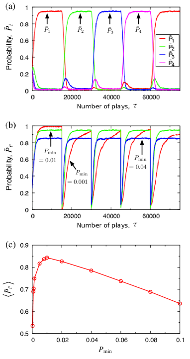
Figure 5: (Color online) Simulation results of the 4-armed bandit problem in a non-stationary environment where the mean rewards are cyclically changed at a constant interval of $T=15000$ steps. (a) Selection probability of arm $i$, where $P_{\text{min}}=0.01$ was used. The best arm is swapped in response to periodic changes in the mean reward. (b) Selection probability of the best arm, $\mbox{$\bar{P}$}_{i^{*}}$, where the red, green, and blue curves represent the results for $P_{\text{min}}=0.001$, $0.01$, and $0.04$, respectively. (c) Relation between the mean of $\left<\mbox{$\bar{P}$}_{i^{*}}\right>$ and $P_{\text{min}}$.

The time evolution of the average selection probability of each arm, $\mbox{$\bar{P}$}_{i}$, when $P_{\text{min}}=0.01$ is shown in Fig. 5(a), where the best arm is switched every $15000$ steps. Immediately after the environmental changes, competition has arisen, and then, the system eventually finds the best arm during each term.

Fig. 5(b) shows the time evolution of the selection probability of the best arm, $\mbox{$\bar{P}$}_{i^{*}}$, with different values of $P_{\text{min}}$. The maximum value of $\mbox{$\bar{P}$}_{i^{*}}$ can be approximately given as $1-(N-1)P_{\text{min}}$, resulting in low optimality for a too large $P_{\text{min}}$, whereas a too small $P_{\text{min}}$ makes the adaptive best arm identification difficult. To investigate the balance between the optimality and adaptability, we calculated the mean value of $\mbox{$\bar{P}$}_{i^{*}}$ over time from $2T$ to $5T$:

$$\left<{\mbox{$\bar{P}$}}_{i^{*}}\right>=\frac{1}{3T}\int^{5T}_{2T}\mbox{$\bar{P}$}_{i^{*}}(t)\ \text{d}{t}.$$ (21)

As can be seen in Fig. 5(c), a smaller value of $P_{\text{min}}$ produces a larger $\left<{\mbox{$\bar{P}$}}_{i^{*}}\right>$, but in the range where $P_{\text{min}}<0.01$, $\left<{\mbox{$\bar{P}$}}_{i^{*}}\right>$ rapidly decreases. Thus, under this setting, $\left<{\mbox{$\bar{P}$}}_{i^{*}}\right>$ has a peak value of approximately $P_{\text{min}}=0.01$.

The simulation results in this appendix can be interpreted as follows: the adaptability is maximized by preventing extinction of all species, even though some of them are not optimal in a certain environment, from the perspective of the “winner-take-all” competition mechanism in ecosystems. This interpretation is reminiscent of the ecosystem stability exerted by natural biodiversity (species richness). Though the actual effect of biodiversity on the stability of ecosystems is more complicatedPennekamp2018Biodiversity , this type of analogy might provide a new insight into the field of reinforcement learning.

References

- (1) P. Agarwal and S. Mehta, Int. J. Comput. Appl. 100, 14 (2014).
- (2) J. H. Holland, R. E. Nisbett, K. J. Holyoak, and P. R. Thagard, Induction: Processes of Inference, Learning, and Discovery (MIT Press, Cambridge, 1989).
- (3) M. Dorigo, V. Maniezzo, and A. Colorni, IEEE Trans. Syst. Man. Cybern. Syst. B 26, 29 (1996).
- (4) D. Karaboga and B. Basturk, J. Global Optim. 39, 459 (2007).
- (5) D. Karaboga and B. Basturk, Appl. Soft Comput. 8, 687 (2008).
- (6) S. Kirkpatrick, C. D. Gelatt, and M. P. Vecchi, Science 220, 671 (1983).
- (7) V. Černý, J. Optim. Theory Appl. 45, 41 (1985).
- (8) R. S. Sutton and A. G. Barto, Reinforcement learning: An introduction (MIT press, Cambridge, 2018) 2nd ed., Chap. 2.
- (9) J.-Y. Audibert and S. Bubeck, COLT - 23th Conference on Learning Theory - 2010, Haifa, 2010, p. 13.
- (10) S.-J. Kim, M. Aono, and M. Hara, Biosystems 101, 29 (2010).
- (11) S.-J. Kim, M. Aono, and E. Nameda, New J. Phys. 17, 083023 (2015).
- (12) M. Naruse, M. Berthel, A. Drezet, S. Huant, M. Aono, H. Hori, and S.-J. Kim, Sci. Rep. 5, 13253 (2015).
- (13) S.-J. Kim, M. Naruse, and M. Aono, Philosophies 1, 245, (2016).
- (14) M. Naruse, Y. Terashima, A. Uchida, and S.-J. Kim, Sci. Rep. 7, 8772 (2017).
- (15) R. Homma, S. Kochi, T. Niiyama, T. Mihana, Y. Mitsui, K. Kanno, A. Uchida, M. Naruse, and S. Sunada, Sci. Rep. 9, 9429 (2019).
- (16) S. A. Baigent, Lotka-Volterra dynamics, an introduction. preprint, University of College, London (2010).
- (17) M. L. Zeeman, Proc. Am. Math. Soc. 123, 87 (1995).
- (18) M. Sargent III, M. O. Scully, and W. E. Lamb, Laser Physics (Addison-Wesley, Reading, 1993), Chap. XI.
- (19) M. Sargent, Phys. Rev. A 48, 717 (1993).
- (20) A. E. Noble, A. Hastings, and W. F. Fagan, Phys. Rev. Lett. 107, 228101 (2011).
- (21) J. Hofbauer and K. Sigmund, Bull. Am. Math. Soc. 40, 479 (2003).
- (22) N. Baba, New Topics in Learning Automata Theory and Applications (Springer-Verlag, Heidelberg, 1985).
- (23) K. S. Narendra, S. Mukhopadyhay, and Y. Wang, arXiv:1510.05034.
- (24) M. Naruse, T. Mihana, H. Hori, H. Saigo, K. Okamura, M. Hasegawa, and A. Uchida, Sci. Rep. 8, 10890 (2018).
- (25) M. Harper, Physica D 240, 1411 (2011).
- (26) O. M. Abou Al-Ola, K. Fujimoto, and T. Yoshinaga, Math. Probl. Eng. 2011, 723509 (2011).
- (27) F. Pennekamp, M. Pontarp, A. Tabi, F. Altermatt, R. Alther, Y. Choffat, E. A. Fronhofer, P. Ganesanandamoorthy, A. Garnier, J. I. Griffiths, S. Greene, K. Horgan, T. M. Massie, E. Mächler, G. M. Palamara, M. Seymour, and O. L. Petchey, Nature 563, 109 (2018).