High-dimensional nonlinear dynamical systems including neural networks can be utilized as a computational resource for information processing. In this sense, nonlinear wave systems are good candidate for such a computational resource. Here, we propose and numerically demonstrate information processing based on nonlinear wave dynamics in microcavity lasers, i.e., optical spatiotemporal systems at a microscale. One of the remarkable features is the ability of high-dimensional and nonlinear mapping of input information into the wave states, enabling efficient and fast information processing at a microscale. We show that the computational capability for nonlinear/memory tasks is maximized at the edge of the dynamical stability. Moreover, we also show that the computational capability can be enhanced by applying a time division multiplexing technique to the wave dynamics; thus, the computational potential of the wave dynamics can sufficiently be extracted even when the number of detectors to monitor the wave states is limited. In addition, we discuss the merging of optical information processing and optical sensing, opening a novel method of model-free sensing by using a microcavity reservoir itself as a sensing element. These results open a way to on-chip photonic computing with high-dimensional dynamics and a novel model-free sensing scheme.

Introduction

Reservoir computing (RC) [1], originally known as an echo state network [2] or a liquid state machine [3], is a computational paradigm using high-dimensional dynamical systems, and it has been regarded as a powerful tool for solving highly-complex and abstract computational tasks. The computational paradigm has recently been implemented in a variety of physical systems or devices, such as optoelectronic systems [4], photonic systems [5], memristors [6], spin systems [7], and soft materials [8]. (See Ref. [9] for a comprehensive review on physical RCs.) In particular, the photonic implementation of RC has been expected to open the path to ultrafast and efficient processing beyond traditional Turing-von Neumann computer architecture [10, 11, 12, 13, 14, 15].

A key principle of the RC is a high-dimensional mapping of the input information based on the high-dimensionality of the reservoir dynamical systems; the computational capability is dependent on the number of linearly independent internal states of dynamical systems in response to an encoded input [16]. Moreover, a nonlinearity and short-term memory effect inherent in dynamical systems also play a crucial role in solving computational tasks requiring nonlinearity or memories. Thus, infinite dimensional nonlinear systems will be good candidates as reservoirs.

One of the representative infinite dimensional systems is a delay system, where reservoir networks can virtually be constructed in a time domain [17]. To date, numerous experimental studies in the photonic RC with delay systems have been performed because of the easy implementation in optoelectronic or photonic systems, such as lasers with delayed feedback [10, 11, 18, 19]. The information processing, including prediction [10] and speech recognition [11], have been demonstrated; however, the drawback is the requirement of long delay lines to make many virtual nodes in the RC, which could lead to impractically large systems, inhibit stable operation , and may prevent practical deployments.

In this study, we propose to use a microcavity laser, i.e., a microscale spatially-extended optical system, as a reservoir. Originally, microcavities have mainly been utilized to realize a low threshold laser source and modify quantum effects by the strong optical confinement effect, which is caused by the difference in refractive indexes between inside and outside the cavity [20]. Then, a various shapes of microcavity lasers, inspired by wave/quantum chaos, have recently been utilized to control the emission properties [21, 22]. An interesting feature of such microcavity lasers is to be able to exhibit a variety of spatiotemporal wave dynamics by the interplay of a gain medium and cavity shape [23, 24]. Unlike the previous works, we utilize such wave dynamics in microcavity lasers driven by an input signal for RCs and numerically demonstrate that the RC-based information processing can efficiently be achieved at a microscale owing to the spatial degrees of freedom based on the high-dimensional dynamics with a long memory effect.

In addition, we discuss the application of the microcavity-based processing by using the sensitivity of wave dynamics in a microcavity to an external perturbation; we propose to use a microcavity as a sensing element as well as a reservoir, resulting in high-dimensional mapping. The merging of optical sensing and the reservoir suggests the possibility of novel sensing without complex post processing and theoretical sensing models. As a proof-of-concept demonstration, we show fast sensing of external reflective index by using the microcavity RC.

Microcavity-based RC

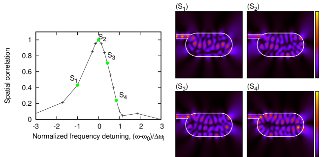
Figure 2: Dependence of excited wave patterns on the input frequency $\omega$. The left figure shows the spatial correlation $C(\omega)=\langle(I_{\omega}-\bar{I}_{\omega})(I_{\omega_{0}}-\bar{I}_{\omega_{0}})\rangle/(\sigma_{\omega}\sigma_{\omega_{0}})$, where $\langle\cdot\rangle$ denotes the spatial average, and $I_{\omega}(\mbox{\bf r})$ represents the intensity pattern excited by the input light with frequency $\omega$. $\bar{I}_{\omega(\omega_{0})}$ and $\sigma_{\omega(\omega_{0})}$ denotes the spatial average and standard deviation. The horizontal axis is the frequency detuning of the input light from a resonant frequency $\omega_{0}$ of the stadium cavity, normalized by the average mode interval $\Delta\omega_{i}$. As seen in this figure, the input frequency affects the wave patterns; thus the input information can be encoded into the wave patterns with the instant frequency of the phase-modulated light. In the simulation, $W_{\infty}=0$ was set.

Figure 1(a) shows a schematic of the proposed system, which consists of a microcavity coupled to an input waveguide and probes (detectors) to make the RC output $\hat{y}$. The microcavity include a nonlinear gain medium, and the cavity shape is designed as the Bunimovich stadium [25], in which ray orbits are proven to be fully chaotic and the corresponding wave patterns are complex (Fig. 1b). An optical signal encoded with a phase modulation is injected from the input waveguide and can reach all parts of the cavity due to the chaotic multiple reflections at the cavity boundary and is nonlinearly amplified by the gain medium. A feature of the stadium cavity is the dependence of the wave pattern on the input frequency; the wave pattern sensitively changes, depending on the input frequency. Actually, as demonstrated in Fig. 2, the spatial correlation between two wave patterns excited by the inputs with frequencies $\omega_{0}$ and $\omega=\omega_{0}+\Delta\omega$ decreases as $\Delta\omega$ increases. This means that the information can be encoded into the wave patterns with the instant frequency by phase-modulating the input light. Then, the gain medium play an important role in adding an additional nonlinearity and memory effect by the amplification. The emitted signals from the cavity are detected at point probes at the sampling time interval $\tau_{s}$. In the simulation, $N$ probes are assumed to be placed around the cavity.

For RC, we consider the linear readout $\hat{y}$ as $\hat{y}(t)=\sum_{i=1}^{M}w_{i}x_{i}(t)$, where $x_{i}$ is the detected intensity at probe $i$, ($i\in\{1,2,\cdots,N\}$), at time $t=n\tau_{s}$ ($n\in\{1,2\cdots,\infty\}$), and $w_{i}$ is a readout weight. The goal of the processing is to approximate a functional relation between input signal $u(n)$ and target signal $y(n)$ by the readout $\hat{y}$. To this end, a finite set of training data $\{u(n),y(n)\}_{n=0}^{T}$ is utilized to determine the readout weights, such that the normalized mean square error $1/T\sum_{n}|y(n)-\hat{y}(n)|^{2}$ is minimized. In the training process, we simply use the least square method.

Results and discussions

To gain an insight into the computational capability of the microcavity-based RC, the numerical simulation was performed by using the Maxwell-Bloch (MB) model, where the gain medium is modeled as a simple two-level system [26]. Whereas the MB model is a simple model of microcavity lasers, the dynamical lasing phenomena can qualitatively be examined [27, 28]. We assumed that the cavity is two-dimensionally extended on a plane, and the electric field is polarized perpendicular to the plane. For generality, all variables were made dimensionless (see Methods for details), and we discuss the RC capability with the dimensionless variables.

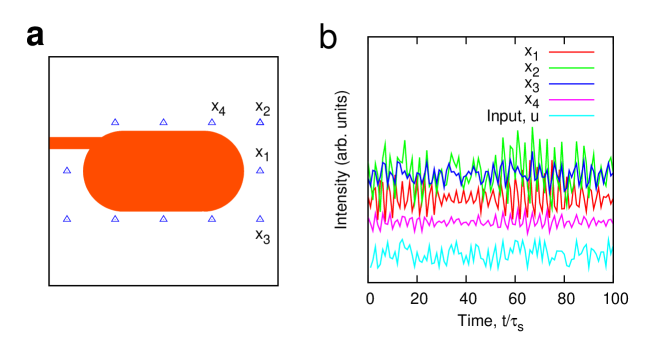
Figure 3: Demonstration of emission dynamics. a. A schematic of the stadium-shaped microcavity laser coupled to an input waveguide. The blue triangles denote the positions of the point probes. b. Intensity signals $x_{i}$ detected by the probes $i=1,2,3$ and 4 when the input light is phase-modulated with a signal $u$.

In the simulations, the refractive index $n_{in}$ inside the cavity was set to be 3.3, the length $L$ of the major axis of the stadium cavity was $\approx$1.67$\lambda$, where $\lambda$ is the wavelength of the input light in vacuum. (If $\lambda=0.85$ $\mu$m, $L$ would be 1.42 $\mu$m.) $\tau_{s}$ was fixed to be close the lifetime $\tau_{c}$ of the cavity without a gain medium. (See Methods for discussions toward actual experiments.) The input information $u(n)$ was encoded in the phase of the input light as $\phi(t)=m_{a}u(n)$, where $m_{a}\approx 0.1$ is the modulation amplitude. $u(n)$ holds for the time interval $\tau_{s}$. The center frequency of the input light was locked to a resonant frequency $\omega_{0}$. Under these conditions, a variety of the intensity signals were measured in response to the modulated signal, as demonstrated in Fig. 3.

Nonlinear-memory capacity.

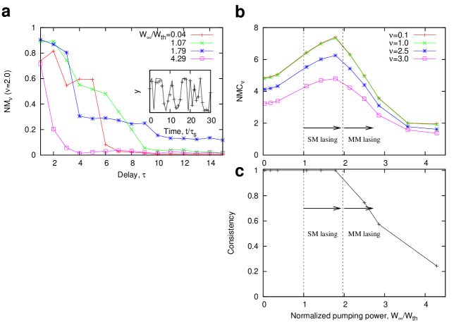
Figure 4: Nonlinear memory capacity of a stadium-shaped microcavity laser. a. $NM_{\nu}(\tau)$ for $\nu=2.0$. $W_{\infty}/W_{th}$ denotes the pumping power normalized by the threshold pumping power. In the simulation, $N=11$ probes were used. The inset shows an example of the RC output $\hat{y}(n)$ for $W_{\infty}/W_{th}\approx 1.79$, denoted by the crosses, and the target signal $y(n)$ for $\nu=2$ and $\tau=1$ (solid black curve) in time $t/\tau_{s}$. b. $NMC_{\nu}$ as a function of the normalized pumping power $W_{\infty}/W_{th}$. When $W_{\infty}/W_{th}>1$, a single mode (SM) lasing starts, and multimode (MM) lasing occurs when $W_{\infty}/W_{th}>1.79$. For the large pumping power $W_{\infty}$, the loss of the input information is compensated and a long memory effect can be achieved. In addition, nonlinear gain saturation plays an important role in introducing additional nonlinearity in the reservoir. However, consistency decreases when MM lasing occurs. Consequently, $NMC_{\nu}$ is maximized around the edge of the stability. c. Consistency as a function of $W_{\infty}/W_{th}$. See Methods for the measurement method of the consistency.

For the evaluation of the computational capability, we use a simple function approximation tasks, $y(n)=\sin[\nu u(n-\tau)]/\nu$, where $\nu$ and $\tau$ are the task parameters that control the required nonlinearity and memory, respectively [29]. The input signal $u(n)$ is an identically distributed random sequence generated from a uniform distribution between $[-1,1]$. The goal of the task is to reproduce the nonlinearly-converted signal $y(n)$ with a delay of $\tau$ (see the inset of Fig. 4a). To evaluate both the ability to adapt nonlinear tasks and memory capacity of the RC, we introduce the correlation between the target signal $y$ and output $\hat{y}$,

$$NM_{\nu}(\tau)=\dfrac{\langle y(n-\tau)\hat{y}(n)\rangle^{2}}{\sigma^{2}_{y}\sigma_{\hat{y}}^{2}},$$ (1)

where $\langle\cdot\rangle$ is the mean over time step $n$, $\sigma_{z}$ denotes the standard deviation of $z=y$ or $\hat{y}$. Then, the nonlinear-memory capacity is defined as the sum of $NM_{\nu}(\tau)$, with $\tau$ going to infinity:

$$NMC_{\nu}=\sum_{\tau=0}^{\infty}NM_{\nu}(\tau).$$ (2)

$NMC_{\nu}$ corresponds to the linear memory capacity $MC$ in the limit of $\nu\rightarrow 0$ [30]. With the nonlinear-memory capacity $NMC_{\nu\neq 0}$, we can both evaluate the nonlinearity and memory effects in microcavity lasers at the same time.

We examined the lasing dynamics in the stadium cavity and obtained $NMC_{\nu}$ from the intensity signals detected by each probe. Figure 4 shows the numerical results of $NM_{\nu}(\tau)$ and $NMC_{\nu}$ with various values of the pumping power $W_{\infty}$ in the gain medium (see Methods for $W_{\infty}$). As shown in Fig. 4a, $NM_{\nu}$ decreases with increasing $\tau$, but the decrease becomes moderate by increasing $W_{\infty}$ in a range of $0\leq W_{\infty}\leq 1.79W_{th}$, where $W_{th}$ denotes the threshold pumping power. The pumping compensates the loss of the input information by the nonlinear amplification effect in the gain medium, and the reservoir (cavity) can have a longer memory and becomes adaptive to nonlinear tasks. Accordingly, $NM_{\nu}$ and the resulting $NMC_{\nu}$ increases with increasing $W_{\infty}$ (Fig. 4b). However, when $W_{\infty}>1.79W_{th}$, multimode lasing occurs and $NMC_{\nu}$ decreases. Consequently, $NMC_{\nu}$ of the RC with the microcavity laser is maximized around the edge of the phase transition, $W_{\infty}/W_{th}\approx 1.79$.

The decrease of $NMC_{\nu}$ is explained by the loss of the consistency [31], or the so-called echo-state property [2], which is an important condition for RC [29, 32]. In the multimode lasing regime, the spontaneous multi-modal oscillations appear, leading to different results even from the same input, depending on the initial states of the reservoir; thus, the appearance of the irreproducibility prevents consistent processing of the input information. We measured the consistency, which is defined by the mean correlation between the output signals starting from two different initial states. (see Method for the detail.) As shown in Fig. 4c, the decrease of the consistency is linked to the degrade of $NMC_{\nu}$.

As shown in these results, the effects of the gain medium as well as the high-dimensionality of the wave states play a crucial role in enhancing the computational capability in the RC frameworks. We emphasize that the compensation of the short memory inherent in compact RC systems and additional nonlinearity caused by the interaction with the gain medium are advantage, compared to conventional passive photonic integrated RC [12, 14, 15], where nonlinearity is introduced only in the measurement process.

Effect of cavity shapes.

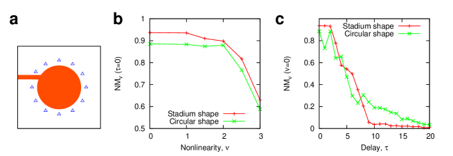
Figure 5: Performance comparison of stadium- and circular-shaped lasers. a. A schematic of the circular-shaped laser coupled to an input waveguide. The blue triangles denote the positions of the point probes. b. Adaptivity to nonlinear tasks, where $NM_{\nu}$ with $\tau=0$ is shown in a function of the nonlinear parameter $\nu$. c. Linear memory capacity. $NM_{\nu=0}(\tau)$ is shown as a function of the delay parameter $\tau$. In b and c, the performances of the stadium- and circular-shaped lasers are compared under the same input condition, same number of probes $N=11$, and same pumping condition in a single-mode lasing (consistency) regime. For nonlinear tasks, the $NM_{\nu}$ of the stadium-shaped laser is higher than that of the circular-shaped laser, as shown in b. However, the circular-shaped laser outperforms the stadium-shaped laser for tasks requiring long memory $\tau\gg 1$, as shown in c.

The cavity shapes play a crucial role in the quality of the light confinement and the wave dynamics, resulting from the multiple reflections inside the cavity. In the stadium cavity, the chaotic multiple reflections will lead to efficient wave mixing dynamics, enabling high-dimensional mapping of the input information into complex wave patterns, as demonstrated in the previous subsection. To gain a further insight into the effect of the wave-chaotic cavity on the RC performance, we also numerically examined the laser dynamics in a non-chaotic cavity, where the internal ray orbits do not exhibit chaos. As a non-chaotic cavity, we choose a circular-shaped cavity (Fig. 5a) and compared the RC performance with that obtained in the stadium-shaped lasers with the same area and same pumping power condition in a consistency regime.

Figure 5b shows the performance comparison for nonlinear tasks, where $NM_{\nu}$ is shown as a function of nonlinear parameter $\nu$ when delay $\tau=0$. Clearly, $NM_{\nu}$ of the stadium-shaped laser can outperform that of the circular-shaped laser for all values of $\nu$, which may partly be attributed to a strong wave mixing effect in the stadium cavity. As shown in Fig. 5c, however, for the tasks requiring memory with the delay parameter $\tau\gg 1$, the $NM_{\nu}$ of the circular-shaped laser is relatively higher than that of the stadium-shaped laser because the circular cavity has longer cavity-lifetime, (lower loss rate) [22]. These results suggests the trade-off between the cavity shapes exhibiting a long-memory effect and nonlinearity. In terms of ray-wave correspondence [33], the effect of the cavity shape becomes more dramatic for a larger value of the size parameter defined by $n_{in}L/\lambda$; thus, it is expected to lead to a larger difference in the RC performance. The investigation along this line will be an important issue in the RC.

Enhancing the computational capability.

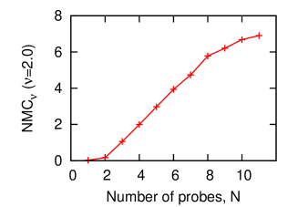
Figure 6: $N$-dependence of RC performance. $NMC_{\nu}$ vs. the number of probes $N$, corresponding to the number of the reservoir nodes. In the simulation, the minimum distance between the probes is set to be close to the wavelength inside the cavity, so as to obtain independent responses to the input signals. $NMC_{\nu}$ increases as $N$ increases.

In the RC, the computational capability generally increases as the number of independent reservoir nodes increases because the expressivity increases [16]. In our case, the number of the reservoir nodes used for the output $\hat{y}$ correspond to the number $N$ of the signals detected by the probes. As clearly depicted in Fig. 6, the $NMC_{\nu}$ actually turned out to be proportional to the number of the probes $N$. This may be one of the merit of using the high-dimensional wave dynamics in the sense that the capability is enhanced by increasing the number of the probes; however, the number $N$ will be limited by the cavity size and wavelength because the similar output are obtained if the minimum distance between the probes is much shorter than the wavelength. We roughly estimate the maximum number of the probes (effectively corresponding to the maximum number of the measurable nodes) as the ratio of the perimeter $P=(\pi/2+1)L$ of the stadium cavity to characteristic wavelength $\lambda/n_{in}$ inside the cavity with $n_{in}$, $N\sim(\pi/2+1)n_{in}L/\lambda$, considering that the spatial autocorrelation of the wave patterns typically is sufficiently small for a spatial scale larger than $\lambda$. For example, $N\approx 1600$ nodes can potentially be used in 0.013 mm² footprint for $L=160\mu$m, $\lambda=0.85$ nm, $n_{in}=3.3$. This suggests that larger sized cavity will have a larger computational capability. We emphasize that the potential of implementing such high-density and large-scale (virtual) nodes is a unique characteristic of the wave dynamical RC, which is different from conventional photonic integrated RC [12], consisting of multiple elements.

Using spatiotemporal dynamics for RC.

As discussed in the previous subsection, the computational capability depends on the number of the probes $N$ in the present RC. In the actual implementation, however, it may be practically difficult to place a large number of probes (or detectors) around the cavity. To overcome the problem, it should be noted that the dynamical information is included in a delayed sequences obtained from a few observables [34]. This suggest the possibility that even when only a few observables are utilized, the dynamical information can be extracted from the dynamics of a few observables. In addition, the use of mask signals can make a rich variety of the reservoir responses [17]. We use virtual nodes in a time domain for RC with a time-multiplexing method used in delay-based RCs [17, 30]. First, an input signal is multiplied by a mask signal with a period of $T_{m}$. Then, each response $x_{i}$ to the signal at probes $i$ is sampled at $M$ times with a sampling interval $\tau_{s}(=T_{m}/M\approx\tau_{c})$. We describe the response $x_{i}$ at time $t=nT_{m}+j\tau_{s}$ $(j\in[1,2,\cdots,M])$ as the node labeled by $i$ and $j$, i.e., $x_{ij}(n)=x_{i}(nT_{m}+j\tau_{s})$. Moreover, we use the past node response $x_{ij}(n-k)$, ($k\in\{1,2,\cdots,K\}$) Finally, the output signal $\hat{y}(n)$ at time step $n$ is calculated as

$$y(n)=\sum_{i=1}^{N}\sum_{j=1}^{M}\sum_{k=0}^{K}w_{ijk}x_{ij}(n-k),$$ (3)

where $w_{ijk}$ is an optimal weight, which can be obtained by using the least-squares method.

An example of the time-multiplexing method for $M=10$ is shown in Fig. 7a, where the input information $u$ holds for the period $T_{m}$, and the colored random signals with the period $T_{m}$ is used as the mask signal because the use of colored noise or chaotic oscillation as the mask signals will lead to a good RC performance [35]. Figures 7b and c show the $NM_{\nu}(\tau)$ and $NMC_{\nu}$, respectively, for various values of $M$ and $K$. When comparing the red curve ($M=1$ and $K=0$) and green curve ($M=10$ and $K=0$) in Fig. 7b, one can see that $NM_{\nu}$ is enhanced for nonlinear tasks in $\tau<5$ as $M$ increases, whereas the memory capacity decreases in a region of $\tau>5$. The memory loss is compensated by increasing the number of the past nodes $K$; thus, $NMC_{\nu}$ can be enhanced when $M$ and $K$ both increase, as shown by the blue curve ($M=10$ and $K=5$) and pink curve ($M=10$ and $K=10$) in Fig. 7b. We find that with the time-multiplexing method of $M=10$ and $K=5$, $NMC_{\nu}$ for only a single probe $N=1$ can be larger than $NMC_{\nu}$ without the time-multiplexing method (Fig. 7c). This time-multiplexing method is effective to achieve high RC performance even when the number of the probes is limited in physical reservoirs.

Sensing applications.

Physical RC frameworks generally suggest that physical systems responding to input signals themselves can be utilized as information processing systems. This implies that when the physical systems is perturbed by an external stimulus (e.g., environmental changes), the system itself can also be utilized to detect the external stimulus with an appropriate training process. Here, we consider microcavities to detect an environmental physical quantity in the RC scheme and demonstrate the identification of refractive index $n_{out}$ outside the cavity, i.e., refractometric sensing.

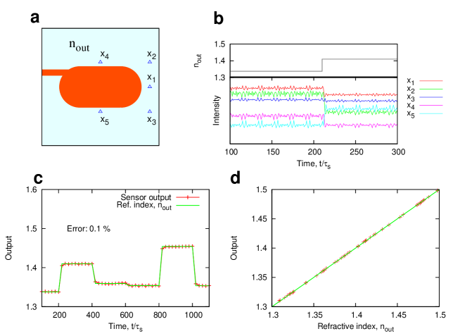
Figure 8: Sensing of environmental refractive index. a. Stadium cavity used for the sensing of refractive index $n_{out}$. The phase-modulated light is injected into the stadium cavity, and five signals detected by probes denoted by the blue triangles are used for the output $\hat{y}$. For passive cavity sensing, $W_{\infty}/W_{th}=0$ was set. b. An example of the probe signal $x_{i}$ for the phase-modulated light (input). $x_{i}$ changes when $n_{out}$ changes at time $t/\tau_{s}=215$. c. The output signal $\hat{y}$ after training. $\hat{y}$ can identify $n_{out}$, with 0.1 $\%$ error, even when it rapidly changes. d. The trained output $\hat{y}$ vs. refractive index $n_{out}$.

As a simple demonstration, we consider the case when a stadium microcavity is surrounded by a medium with refractive index $n_{out}$, as shown in Fig. 8a. A randomly phase-modulated light is injected to the stadium cavity and the emission from the cavity are detected with the five probes ($N=5$). When the external refractive index $n_{out}$ changes, the phases of the reflection/transmission and the coupling to the probes are changed; consequently, the detected intensity $x_{i}$ at the probe $i$ are also changed (Fig. 8b). We use $x_{ij}=x_{i}(nT_{m}+j\tau_{s})$ ($j=1,\cdots,M$) responding to the phase-modulated light to form $\hat{y}=\sum_{i,j}w_{ij}x_{ij}$. Our purpose is to identify the surrounding refractive index $n_{out}$ from the output $\hat{y}$ after the training of $w_{ij}$ to minimize $\|n_{out}-\hat{y}\|$. In the training process, we used 100 datasets of $\{x_{1}(t),\cdots,x_{N}(t)$,$n_{out}\}$, where $n_{out}$ was randomly chosen in a region of $1.3\leq n_{out}\leq 1.5$.

Figure 8c shows the trained output $\hat{y}$, where it is assumed that $n_{out}$ randomly changes in time. Clearly, $\hat{y}$ follows the changes of the index $n_{out}$ with the error of 0.1 $\%$, even when $n_{out}$ is rapidly changed in a timescale of $\tau_{s}\approx\tau_{c}$. Consequently, $n_{out}$ can be identified with low errors, as shown in Fig. 8d. We remark that the memory of the reservoir (cavity) does not play an essential role in this sensing task. In this sense, the proposed learning-based sensing scheme is related to extreme learning machine (ELM) [30] as well as RC.

We emphasize that the proposed method do not need any precise sensing model, high-quality microcavity, as well as complex post processing, unlike the previous works on microcavity sensor [36, 37], where the shift of the resonant frequency in a microcavity due to the change of the refractive index has been measured from the transmission or reflection spectra.

The results presented in this subsection suggest that with the merging of the optical sensing and learning-based processing, a model-free detection of the external refractive index $n_{out}$ is achieved at a rate of $1/\tau_{c}$.

Summary

In the present work, we proposed and demonstrated RC based on nonlinear wave dynamics in a microcavity laser. One of the merits of using the wave dynamics is to enable high-dimensional mapping of the input information into the wave patterns, after the nonlinear amplifition in the gain medium; consequently, a number of the signals detected by each probe can be used as nonlinear nodes for high RC performance. We emphasize that the high-dimensional mapping into the wave patterns is spontaneously processed with low energy loss by natural multiple reflections, at a ultimate short timescale, which may be of the order of a the cavity lifetime $\tau_{c}$, suggesting the potential for photonic parallel information processing.

Then, we also proposed to apply a time-multiplexing encoding technique to the wave dynamics and demonstrated the enhancement of the computational capability. This method will be useful for the situation when only a few detectors are available due to a physical constraint, and beyond the example of the microcavity lasers, it will be applicable for any physical RC systems with spatial degree of freedom but only with a few detectors.

Lastly, we discussed the sensing applications of the microcavity-based RC, where the microcavity is used as sensing elements as well as a reservoir. The combination of the optical sensing and RC will be useful for model-free identification of physical quantities.

These results opens a way to utilize complex wave dynamical systems at a microscale for fast photonic information processing and will shed light on a novel potential toward model free sensing with the concept of RC.

Method

Maxwell-Bloch model in microcavity lasers

We assume that the thicknesses of microcavities are much smaller than their in-plane dimensions, and microcavities were treated as two-dimensional objects by applying effective refractive indices $n_{in}$. To describe the light-matter interaction, we used the Maxwell-Bloch (MB) model, where the gain medium inside the cavity is modeled as a two-level system. The Maxwell-Bloch model is a simple model to describe the laser dynamics but can quanlitatively reproduce lasing phenomena in two-dimensional microcavity lasers [26, 27]. The normalized Maxwell-Bloch model is given by :

$$\dfrac{\partial^{2}E}{\partial t^{2}}=\dfrac{1}{\epsilon}\nabla^{2}_{xy}E-\sigma\dfrac{\partial E}{\partial t}-\Theta\dfrac{4\pi}{\epsilon}\frac{\partial^{2}}{\partial t^{2}}\left(\rho+c.c\right),$$ (4)

$$\dfrac{\partial\rho}{\partial t}=-\left(\gamma_{\perp}+i\Delta_{a}\right)\rho+\gamma_{\perp}WE,$$ (5)

$$\dfrac{\partial W}{\partial t}=-\gamma_{\parallel}\left(W-W_{\infty}\right)-2iE\gamma_{\parallel}\left(\rho-\rho^{*}\right),$$ (6)

where space and time are made dimensionless by the scale transformations $\omega_{s}x/c\rightarrow x$ and $\omega_{s}t\rightarrow t$, respectively. $\omega_{s}$ is a reference frequency close to the transition frequency $\omega_{a}$ of the two-level gain medium. In Eqs. (4)–(6), $E$, $\rho$, $W$, and all of the other parameters are also made dimensionless. The normalization is similar to that reported in Ref. [38]. $\epsilon=n_{r}^{2}$ is the relative permittivity, where the refractive index $n_{r}$ is $n_{in}$ inside the cavity and waveguide, whereas it is $n=n_{out}$ outside the cavity and waveguide. $\sigma$ represents the background absorption inside the cavity. $\Theta(x,y)$ is a step function; $\Theta$ is 1 inside the cavity and zero outside the cavity. $\Delta_{a}=\omega_{a}/\omega_{s}$ represents the normalized gain center. The two relaxation parameters, $\gamma_{\perp}$ and $\gamma_{\parallel}$, are the transverse and longitudinal relaxation rates, respectively. $W_{\infty}$ represents the pumping power.

The Maxwell Eq. (4) was simulated by the finite-difference time-domain (FDTD) method, where a perfect matched layer (PML) was introduced near the boundary of the calculation space to absorb the emission light. See Ref. [26] for the simulation method.

In the stadium cavity shown in Fig. 1, the radius $R$ of the half circle and major axis length $L=4R$ of the stadium were set $12.25/\sqrt{2}$ and $49/\sqrt{2}$ in a unit of $c/\omega_{0}$, where $\omega_{0}$ is the input angular frequency, and $c$ is the light velocity in vacuum. The actual $L$ would be $\sim$1.42 $\mu m$ if $n_{in}=3.3$ and wavelength $\lambda=0.85\mu$m. Although $L$ is shorter than that of a standard microcavity, we restrict ourselves to the cases of the short length due to the lack of the computational power. We emphasize that the similar results can be essentially obtained in the cases of the longer lengths.

The values of the remaining parameters are: $n_{in}=3.3$, $\sigma=10^{-3}$, $\Delta_{a}=1$, $\gamma_{\perp}=0.1$, $\gamma_{\parallel}=10^{-4}$. $n_{out}$ was set to be 1 for the results shown in Figs. 1–7, whereas in Fig. 8, $n_{out}$ is changed in a range of $1.3\leq n_{out}\leq 1.5$. We confirmed that these parameter values do not essentially affect the RC performance.

Incident wave

The incident light $E_{in}$ is phase-modulated with the input signal $u(n)$, and it is injected to the cavity via the input waveguide shown in Fig. 1,

$$E_{in}=A\psi\cos(\omega_{0}t+\phi(t)),$$ (7)

where $A$ is the amplitude, $\psi$ is the lowest-order waveguide mode, $\omega_{0}$ is the center frequency of the input light, and it is tuned to a resonant frequency of the stadium cavity. The amplitude $A$ is given such that the injection locking to the lasing mode with frequency $\omega_{0}$ is achieved when $W_{\infty}/W_{th}>1$. All results presented in this paper are given under the injection locking condition.

$\psi(t)=\psi_{0}Mask(t)u(t)$ is the modulated phase, where $\psi_{0}$ is the modulation amplitude, $Mask(t)$ and $u(t)$ represents the mask signal and the input signal at time $t$, respectively. $u(t)$ holds for a time interval $\tau_{s}\approx\tau_{c}=143/\omega_{0}$, where $\tau_{c}$ is the cavity lifetime. For a small cavity with $R=12.25/\sqrt{2}$ and input wavelength $\lambda=0.85$ nm, the cavity lifetime $\tau_{c}$ is close to 0.1 ps. Thus, the sampling at the interval $\tau_{s}\approx\tau_{c}$ is unrealistic; however, we remark that the problem can be moderate for a large cavity because $\tau_{c}$ can increase with increasing $R$ [22].

As for the mask signal, $Mask(t)$ is a colored noise signal with a the decay rate of $1/\tau_{c}$, which is repeated with a time interval $T_{m}$. The use of such a colored noise can efficiently excite the modes used for the RC [35].

Estimation of parameter values toward actual experiments

In this study, we have restricted ourselves to the case of the small cavity of $L\approx 1.67\lambda$ and owing to the limitation of our computational power. However, we remark that the results presented in this paper do not essentially depends on the cavity size in the normalized form; thus, the real values in actual experiments can be estimated. For example, when $L=100\mu$m, average mode interval $\Delta\omega_{i}/(2\pi)$ will be of the order of gigahertz [28]. The photon lifetime $\tau_{c}$ in the stadium cavity (without the waveguide) is estimated as 28 ps, and it can be changed by the amplification due to the gain medium. Then, the sampling rate $\tau_{s}$ can be of the order of $\tau_{c}$, which can be set in an actual experiment. In addition, we also remark that for a large cavity with $L=100\mu$m, the probes or single-mode waveguides coupled to detectors can be relatively easy to be placed around the cavity.

Consistency

Consistency is the similarity of the response outputs for a repeated drive signal, and it is one of the important properties of RC [31]. The consistency can be measured by the correlation between the two response outputs obtained from different initial conditions. We measured the consistency of the wave dynamics in microcavity lasers driven by the input light $E_{in}$ as follows:

$$C=\dfrac{1}{N}\sum_{i=1}^{N}C_{i},$$ (8)

where

$$C_{i}=\dfrac{\langle(x^{(1)}_{i}-\bar{x}^{(1)}_{i})(x^{(2)}_{i}-\bar{x}^{(2)}_{i})\rangle}{\sigma_{i,1}\sigma_{i,2}}.$$ (9)

$x_{i}^{(j)}(t)$ denotes the intensity signal detected by the probe $i$, which is obtained from an initial state labeled by $j$. $\langle\cdot\rangle$ denotes the time average. $\bar{x}^{(j)}_{i}$ and $\sigma_{i,j}$ denote the time average and standard deviation of $x_{i}^{(j)}$, respectively. By the definition, $C$ is in the range $-1\leq C\leq 1$, and it takes the maximum $C=1$ when the two signals are identical, i.e., $x_{i}^{(1)}(t)=x_{i}^{(2)}(t)$.

Author contributions

S.S. and A.U. conceived the numerical experiments. S. S. conducted the numerical simulation and analyzed the results. S.S. mainly wrote the paper, and all authors contributed to the preparation of the manuscript.

Additional information

Competing interests: The authors declare no competing interests.

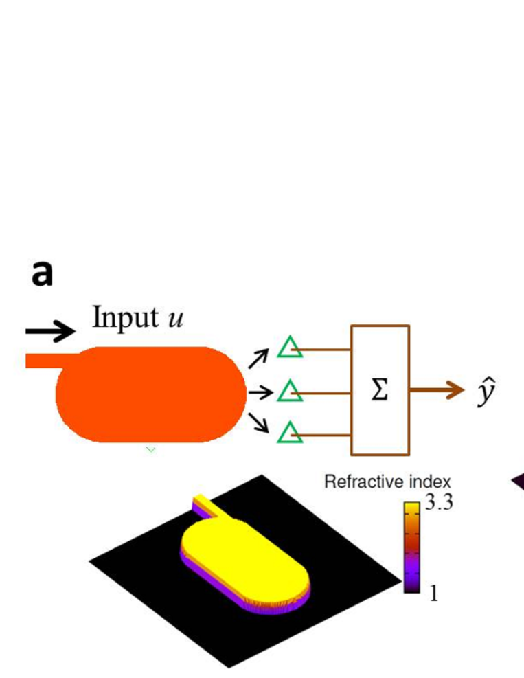
Figure 1: Microcavity laser for RC. a. Schematic of RC using a microcavity laser. The cavity shape is designed as the Bunimovich’s stadium, known as a chaotic cavity and the cavity is coupled to an input waveguide. The incident light encoded by the signal $u$ is injected to the cavity, and the emitted light intensities are detected by the probes, represented by the green triangles, and they are used for the output $\hat{y}$. The lower figure in a shows the refractive index distribution of the stadium cavity coupled to an input waveguide. $n_{in}=3.3$ and $n_{out}=1.0$ denote the refractive indeces inside and outside the cavity and waveguide, respectively. b. An example of the wave patterns responding to the input light, the frequency of which is tuned to a resonant frequency of the cavity $\omega_{0}$. The boundary of the microcavity coupled to the waveguide is represented by the white curves. The green triangles represent the point probes to detect the emission from the microcavity lasers. In the simulation, the normalized pumping power $W_{\infty}/W_{th}\approx 1$ was set, where $W_{th}$ is the threshold pumping power.

Figure 7: Information processing based on the time-multiplexing method. a. An example of time-multiplexing encoding for $M=10$, where a colored random signal with period $T_{m}$ is used as the mask signal. A variety of reservoir responses (e.g., $x_{1}$) are obtained by the mask signal and input $u$. b. $NM_{\nu}$ as a function of the delay parameter $\tau$. The $NM_{\nu}$ is enhanced by increasing both $M$ and $K$. c. $NMC_{\nu}$ vs. the number of probes $N$, corresponding to the number of the reservoir nodes. $NMC_{\nu}$ can increase as $N$, $M$, and $K$ increase. Consequently, the large $NMC_{\nu}$ is achieved by the time-multiplexing method even when the number of probes is limited. In a.-c., $W_{\infty}/W_{th}=1.43$. In a. and b., $N=11$.

References

- [1] Verstraeten, D., Schrauwen, B., D’Haene, M., Stroobandt, D. An experimental unification of reservoir computing methods. Neural. Netw. 20, 391 (2007).
- [2] Jaeger, H. Haas, H. Harnessing nonlinearity: predicting chaotic systems and saving energy in wireless communication. Science 304(5667), 78-80 (2004).
- [3] Maass, M., Natschlager, T., Markram, H. Real-time computing without stable states: a new framework for neural computation based on perturbations. Neural Comput. 14(11), 2531-2560 (2002).
- [4] Paquot, Y. et al.Optoelectronic reservoir computing. Sci. Rep. 2(1), 287 (2012).
- [5] Van der Sande, G., Brunner, D., Soriano, M. C. Advances in photonic reservoir computing. Nanophotonics 6(3), 561-576 (2017).
- [6] Du, C., Cai, F., Zidan, M. A., Ma, W., Lee, S., H. Lu, W. D. Reservoir computing using dynamic memristors for temporal information processing. Nat. Commun. 8, 2204 (2017).
- [7] Nakane, R., Tanaka, G., Hirose, A. Reservoir Computing With Spin Waves Excited in a Garnet Film. IEEE Access 6, 4462-4469 (2018).
- [8] Nakajima, K., Hauser, H., Li, T., Pfeifer, R. Information processing via physical soft body. Sci. Rep. 5, 10487 (2015).
- [9] Tanaka, G. et al. Recent Advances in Physical Reservoir Computing: A Review. Neural Networks 115, 100-123 (2019).
- [10] Brunner, D., Soriano, M. C., Mirasso, C. R., Fischer, I. Parallel photonic information processing at gigabyte per second data rates using transient states. Nat. Commun. 4, 1364 (2013).
- [11] Larger, L. et al. High-Speed Photonic Reservoir Computing Using a Time-Delay-Based Architecture: Million Words per Second Classification. Phys. Rev. X 7, 011015 (2017).
- [12] Vandoorne, K. et al. Experimental demonstration of reservoir computing on a silicon photonics chip. Nat. Commun. 5, 3541 (2014).
- [13] Takano, K. et al. Compact reservoir computing with a photonic integrated circuit. Opt. Express 26(22), 29424-29439 (2018).
- [14] Laporte, F., Katumba, A., Dambre, J., Bienstman, P. Numerical demonstration of neuromorphic computing with photonic crystal cavities. Opt. Express 26(7), 7955-7964 (2018).
- [15] Sunada, S., Arai, K., Uchida, A., Wave dynamical reservoir computing at a microscale. Proc. of 2018 International Symposium on Nonlinear Theory and Its Applications (NOLTA 2018) 1, 154-155 (2018).
- [16] Dambre, J., Verstraeten, D., Schrauwen, B., Massar, S. Information Processing Capacity of Dynamical Systems. Sci. Rep. 2, 514 (2012).
- [17] Appeltant, L. et al. Information processing using a single dynamical node as complex system. Nat. Commun. 2, 468 (2011).
- [18] Martinenghi, R., Rybalko, S., Jacquot, M., Chembo, Y. K., Larger, L., Photonic nonlinear transient computing with multiple-delay wavelength dynamics. Phys. Rev. Lett. 108(24), 244101 (2012).
- [19] Duport, F., Schneider, B., Smerieri, A., Haelterman, M., Massar, S. All-optical reservoir computing. Opt.Express 20(20), 22783-22795 (2012).
- [20] Chang, R. K. Campillo, A. L. (eds) Optical Processes in Microcavities. (World Scientific, New York, 1996).
- [21] Nöckel, J. U. Stone, A. D., Ray and wave chaos in asymmetric resonant optical cavities. Nature 385, 45-47 (1997).
- [22] Cao, H., Wiersig, J. Dielectric microcavities: Model systems for wave chaos and non-Hermitian physics. Rev. Mod. Phys. 87, 61 (2015).
- [23] Harayama T., Shinohara, S. Two-dimensional microcavity lasers. Laser Photonics Rev. 5, 247 (2011).
- [24] S. Bittner, S. Guazzotti, Y. Zeng, X. Hu, H. Y?lmaz1, K. Kim, S. S. Oh, Q. J. Wang, O. Hess, and H. Cao, “Suppressing spatiotemporal lasing instabilities with wave-chaotic microcavities,” Science 361(6408), 1225-1231 (2018).
- [25] Bunimovich, L. A. On the ergodic properties of nowhere dispersing billiards. Commun. Math. Phys. 65(3), 295-312 (1979).
- [26] Harayama, T., Sunada, S., Ikeda, K. S. Theory of two-dimensional microcavity lasers. Phys. Rev. A 72, 013803 (2005).
- [27] Harayama, T., Fukushima, T., Sunada, S., Ikeda, K. S. Asymmetric Stationary Lasing Patterns in 2D Symmetric Microcavities. Phys. Rev. Lett. 91, 073903 (2003).
- [28] Sunada, S., Fukushima, T., Shinohara, S., Harayama, T. Stable single-wavelength emission from fully chaotic microcavity lasers. Phys. Rev. A 88, 013802 (2013).
- [29] Inubushi M. Yoshimura, K. Reservoir Computing Beyond Memory-Nonlinearity Trade-off. Sci. Rep. 7(1), 10199 (2017).
- [30] Ortin, S. et al. A Unified Framework for Reservoir Computing and Extreme Learning Machines based on a Single Time-delayed Neuron. Sci. Rep. 5 14945 (2015).
- [31] Uchida, A., McAllister, R. Roy, R. Consistency of Nonlinear System Response to Complex Drive Signals. Phys. Rev. Lett. 93, 244102 (2004).
- [32] Nakayama, J., Kanno, K., Uchida, A., Laser dynamical reservoir computing with consistency: an approach of a chaos mask signal. Opt. Express 24(8), 8679-8692 (2016).
- [33] Harayama, T., Shinohara, S. Ray-wave correspondence in chaotic dielectric billiards. Phys. Rev. E 92(4), 042916 (2015).
- [34] Takens, F. Detecting strange attractors in turbulence. In D. A. Rand and L.-S. Young (ed.). Dynamical Systems and Turbulence, Lecture Notes in Mathematics, 898 Springer-Verlag. 366–381 (1981).
- [35] Kuriki, Y., Nakayama, J., Takano, K., Uchida, A. Impact of input mask signals on delay-based photonic reservoir computing with semiconductor lasers. Opt. Express 26(5), 5777-5788 (2018).
- [36] Vollmer F., Yang, L. Review label-free detection with high-Q microcavities: a review of biosensing mechanisms for integrated devices. Nanophotonics 1, pp. 267-291 (2012).
- [37] Hanumegowda, N., Stica, C., Patel, B., White, I., Fan, X. Refractometric sensors based on microsphere resonators. Appl. Phys. Lett. 87 (2005).
- [38] Pick, A., et al.Ab initio multimode linewidth theory for arbitrary inhomogeneous laser cavities. Phys. Rev. A 91, 063806 (2015).
- [39] Shinohara, S. and Harayama, T., Signature of ray chaos in quasibound wave functions for a stadium-shaped dielectric cavity. Phys. Rev. E 75,036216 (2007).