Reference Models for Lithospheric Geoneutrino Signal
Abstract
Debate continues on the amount and distribution of radioactive heat producing elements (i.e., U, Th, and K) in the Earth, with estimates for mantle heat production varying by an order of magnitude. Constraints on the bulk-silicate Earth’s (BSE) radiogenic power also places constraints on overall BSE composition. Geoneutrino detection is a direct measure of the Earth’s decay rate of Th and U. The geoneutrino signal has contributions from the local (40%) and global (35%) continental lithosphere and the underlying inaccessible mantle (25%). Geophysical models are combined with geochemical datasets to predict the geoneutrino signal at current and future geoneutrino detectors. We propagated uncertainties, both chemical and physical, through Monte Carlo methods. Estimated total signal uncertainties are on the order of 20%, proportionally with geophysical and geochemical inputs contributing 30% and 70%, respectively. We find that estimated signals, calculated using CRUST2.0, CRUST1.0, and LITHO1.0, are within physical uncertainty of each other, suggesting that the choice of underlying geophysical model will not change results significantly, but will shift the central value by up to 15%, depending on the crustal model and detector location. Similarly, we see no significant difference between calculated layer abundances and bulk-crustal heat production when using these geophysical models. The bulk crustal heat production is calculated as terrawatts, which includes an increase of 1 TW in uncertainty relative to previous studies. Future improvements, including uncertainty attribution and near-field modeling, are discussed.
arXiv
Department of Geology, University of Maryland, College Park, MD 20742, USA Department of Geophysics, Faculty of Mathematics and Physics, Charles University, Prague, Czech Republic Department of Earth Sciences and Research Center for Neutrino Science, Tohoku University, Sendai 980-8578, Japan
S. A. Wipperfurthswipp@terpmail.umd.edu
Updated geoneutrino emission model compares results using CRUST2.0, CRUST1.0, LITHO1.0 geophysical models
Observed differences between geoneutrino signals from different geophysical models is negligible
Necessary improvements to geoneutrino modeling are identified
1 Introduction
Estimated at 47 2 terrawatts (TW) J\BPBIH. Davies \BBA Davies (\APACyear2010), the deep Earth’s radiant heat is primarily comprised of two sources: primordial heat remaining from planetary assembly and core formation, and radiogenic heat produced during nuclear decay of the heat-producing elements (HPE: uranium (U), thorium (Th), and potassium (K)). The radioactive isotopes of these elements — 238U (99.3% g/g of U), 235U (0.7%), 232Th (100% g/g of Th), 40K (0.012% g/g of K) — presently account for 99% of Earth’s radiogenic heat due to their long half-lives and high abundances relative to other radiogenic elements.
There are three categories of models which predict the abundance of the HPE’s in the bulk-silicate Earth (BSE; crust + mantle (0.5% and 67% of Earth by mass, respectively)) and therefore the radiogenic heat production within the BSE. Models which predict low heat production (H) from radiogenic decay ( TW) are derived from observations of isotopic similarities between Earth and enstatite chondrite Javoy (\APACyear1999); Javoy \BOthers. (\APACyear2010) or from models of early Earth collisional erosion of an HPE-enriched crust O’Neill \BBA Palme (\APACyear2008). Medium-H models ( TW) are derived from combining observations from chondrites and mantle melting trends of terrestrial samples McDonough \BBA Sun (\APACyear1995); Palme \BBA O’Neill (\APACyear2014). Finally, High-H models ( TW) are derived from simple parameterized mantle convection models Turcotte \BBA Schubert (\APACyear2014). There is inconclusive data to evaluate critically the veracity of each of these three BSE models, therefore there is currently not a precise understanding of the composition and thermal evolution of our planet. The Earth’s stable isotopic composition is most similar to enstatite chondrites (low-H model), and yet it falls outside of the chondritic defined endmembers in a Fe-Mg-Si plot, indicating Earth is not comprised of a single type of chondrite nor a two component mixture McDonough (\APACyear2017). Furthermore, the use of terrestrial samples and observed conservation of chondritic ratios in terrestrial samples yields a BSE composition (medium-H model) with refractory element abundances (including U and Th, but not K) double that estimated from enstatite chondrites alone. Finally, neither the low-H nor medium-H BSE models satisfy some simple parameterized convection models of the Earth which require larger amounts of radiogenic power to avoid a totally molten mantle for a significant amount of Earth history <high-H model;¿davies1980,schubert1980. Overall, the range of heat production in BSE models differ by a factor of three (10 to 30 TW). With the consideration of uncertainties and the removal of the HPE contribution from the accessible and HPE enriched continental crust < TW;¿huang2013, these models differ by a factor of thirty in estimates of the radiogenic power in the modern mantle.
For more than a decade, particle physicists have detected and reported on the Earth’s flux of geoneutrinos — electron antineutrinos () of terrestrial origin produced during decays <;¿[]araki2005. The intensity of the geoneutrino flux is proportional to the concentration and sensitive to the spatial distribution of HPEs inside the Earth relative to the detector’s location. These elusive particles are exceedingly difficult to detect as they are charge-less leptons with small interaction cross sections of the weak interaction <;¿[]vogel1999. Measurement of the geoneutrino flux requires large, underground, scintillation detectors which use the inverse beta decay (IBD) detection process (). The IBD reaction creates two flashes of light, separated in time (200 s) and space (30 cm), which uniquely classifies the event and provides an energy tag identifying the specific geoneutrino source isotope. The IBD reaction requires an kinematic threshold energy of 1.806 MeV due to the larger mass of the products relative to the reactants in the production of ’s. Consequently, only ’s emitted by the decay of U and Th are detectable Araki \BOthers. (\APACyear2005). The detectors also register other electron antineutrinos present in the geoneutrino energy range (1.8–3.3 MeV), including reactor antineutrinos. Detectors are located at 1–2 km deep in the upper crust to shield from cosmogenic muons — the primary non-antineutrino background source. Geoneutrino signals are often reported in terrestrial neutrino units (TNU), with one TNU equal to one IBD detection per 1032 free protons ( one kiloton of liquid scintillator) in one year with 100% detection efficiency of a geoneutrino detector. This unit accounts for differences in detector size and efficiency.
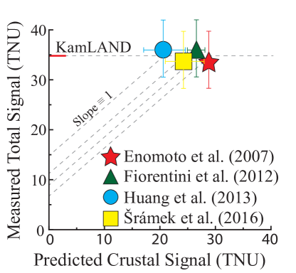
Antineutrino detectors are presently counting geoneutrinos at KamLAND (Kamioka, Japan; 1 kton) and Borexino (Gran Sasso, Italy; 0.3 kton); future detectors include SNO+ (1 kton; online 2019) in Sudbury, Canada, JUNO (20 kton; online 2022) in Guangdong, China, and Jinping (4 kton; unknown start date) in Sichuan, China. Although the Earth is emitting cms, few events are detected annually at KamLAND (∼14/yr) and Borexino (∼4/yr) because of the combined effects of the inverse square law (intensity 1/distance2) and the neutrino’s small interaction cross section. Of these detected events, \citeAaraki2005 estimated that 50% are derived from U and Th in the HPE-enriched upper continental crust within km of the detector (known as “near-field crust”). The remaining signal comes equally from the rest of the continental crust (i.e. the “far-field crust”; km) and the mantle. Consequently, the signal from the crust ( km thick) overpowers that from the more massive mantle ( km thick). In order to determine the mantle contribution to the geoneutrino flux — and therefore the amount of U and Th within the mantle — it is necessary to have precise and accurate estimates of the crustal contribution. Current measurements from KamLAND and Borexino do not yet allow for discernment between different BSE models (Figure 1).

Endeavors to understand the crustal signal constitute a major effort in geoneutrino research. Models of the global crust employ a combination of global and regional seismic and gravity data with extrapolation to areas with minimal available data. Similarly, geochemical data from global compilations representative of sediment, upper, middle, and lower crustal layers are combined with these physical models. These joint models make simplifying assumptions regarding the bulk composition of each layer of the continental crust. Only recently did these geochemical model estimates include lateral and vertical spatial variability, although not in all layers of the crust <e.g.,¿huang2013. A further confounding issue is that there exist different geophysical models of the bulk lithosphere and each yields slightly different geoneutrino estimates. From the variance between these models and lack of direct measurement, it is unclear which model provides a more accurate representation of the crust. For example, estimated signals at KamLAND can vary by as much as 40%, with particular distinction between models produced respectively by the geoscience and physics communities (Figure 2).
This paper aims to update the geoneutrino model of \citeAhuang2013 by application of their geochemical methods to three different geophysical reference models, including a more recent physical model. First, the geophysical structure and properties of the crust from three different geophysical models are described. Geochemical methods are applied to these geophysical models to yield a 3D description of the amount and distribution of [U,Th,K] in the crust. Finally, these combined geophysical and geochemical models are used to calculate the geoneutrino signal at six detector locations. Uncertainties for all input parameters are defined, correlated, and propagated using Monte Carlo methods. Finally, geochemical and geoneutrino signal modeling results are compared and discussed.
2 Geophysical Model

The lithosphere is the outer rigid silicate shell of the Earth and is composed of the thick ultramafic lithospheric mantle and its overlying, relatively thinner and more felsic crust. This crust is either mafic oceanic or intermediate continental crust. In the past few decades authors moved from characterizing the vertical profile of the continental crust as a single bulk layer to a combination of an upper crust and lower crust <e.g.,¿hacker2015, an upper, middle, and lower crust <e.g., CRUST5.1;¿mooney1998, or as a continuously changing density structure <e.g., GEMMA1.0;¿reguzzoni2015. Furthermore, authors have begun to laterally characterize the crust as an assemblage of different groups with similar tectonic and seismic structure, something that has previously been performed <e.g.,¿pakiser1966 but rarely with regard to both lateral and vertical variations. Modern global physical models are constructed using global and local seismic studies, gravity surveys, or a combination of both. The primary utility of global geophysical models is for crustal corrections in mantle tomography Mooney \BOthers. (\APACyear1998) and interpretation of gravity measurements <e.g.,¿reguzzoni2015. These models also serve as the basis for geochemical and geoneutrino modeling.
CRUST5.1 Mooney \BOthers. (\APACyear1998) provided seismic compressional () and shear wave () velocity averages for regions with similar crustal structure in order to extrapolate to regions where there was limited or no data Mooney \BOthers. (\APACyear1998). This model defined the crust as three layers (upper, middle, and lower) with a sediment layer on top. The subsequent family of geophysical models built on CRUST5.1’s data and methods have a generational increase in input data, resulting in resolution changes from CRUST5.1 (5°lat 5°lon, i.e., 2592 tiles laterally) CRUST2.0 <2° 2°, 16200 tiles;¿bassin2000 CRUST1.0 <1° 1°, 64800 tiles;¿laske2013). Of note, CRUST2.0 and CRUST1.0 provide limited transparency of the model inputs or methodology aside from AGU and EGU abstracts, respectively. The most recent iteration of the ”CRUST” family of models, LITHO1.0 (1° 1°) Pasyanos \BOthers. (\APACyear2014), perturbed CRUST1.0 parameters (density, seismic speeds and , layer thickness) to fit a global surface wave dataset and for the first time included lithosphere-asthenosphere boundary (LAB) depths. LITHO1.0 reports and as a continuous probability distribution, while CRUST2.0 and CRUST1.0 report a few discrete velocities within each layer. Recently, \citeAolugboji2017 showed that LITHO1.0 displays a smaller misfit to high-resolution seismic studies in the United States compared to CRUST1.0. CRUST2.0, CRUST1.0, and LITHO1.0 are adopted as the physical basis for our geoneutrino modeling in order to test their effect on modeled outputs. Model parameters relevant to this study are the layer thickness, density, and . These geophysical models are not combined with the more recent GEMMA1.0 (as was done by \citeAhuang2013) due to ambiguity regarding GEMMA1.0’s dependence on the adopted density structure of the crust. However, this also means that we do not have a measure of uncertainty on crustal thickness and must rely on estimates from previous studies (see Section 4). A comparison of the mass and thickness of layers within these models is shown in Table 1, Figure 3 (density and mass comparisons), and Figure 4 (thickness comparisons).

Previous geoneutrino reference models were generally built upon the most recent model available. The first model post the start of geoneutrino measurements at KamLAND was that of \citeAmantovani2004 built using the Preliminary Reference Earth Model <PREM;¿dziewonski1981, followed by the models of \citeAenomoto2007 and \citeAfiorentini2012 for the geoneutrino signal at KamLAND and Borexino (built on the geophysical model CRUST2.0). \citeAhuang2013 is built on a combination of the physical models CRUST2.0, CUB2.0 Shapiro \BBA Ritzwoller (\APACyear2002), and GEMMA1.0 and has been used in the prediction of signals at SNO+ Huang \BOthers. (\APACyear2014); Strati \BOthers. (\APACyear2017) and JUNO Strati \BOthers. (\APACyear2015), among others. Finally, \citeAsramek2016 calculated the signal at Jinping with a model built upon CRUST1.0 Laske \BOthers. (\APACyear2013).
For the purposes of this study LITHO1.0 is re-meshed from its original icosahedron equal-area tesselation (level 7; with 1° spacing) onto a 1°lat 1°lon grid. Similarly, CRUST2.0 is re-meshed into a 1° 1° grid from its previous 2° 2° grid. Re-meshing was necessary to more easily compare modeled outputs. We split the LITHO1.0 and CRUST1.0 tiles into continental and oceanic crust using the crust type characterization from CRUST1.0 and split CRUST2.0 by its own classification. For CRUST1.0 and CRUST2.0, oceanic crust is defined as types A0, A1, B-, V1, Y3 or all A and B types, respectively; these correspond to crustal types labeled ”oceanic”. The final models contain sediment layers (two for CRUST2.0 and 3 for CRUST1.0 and LITHO1.0), upper, middle, and lower crust, and lithospheric mantle. Sedimentary thickness within the ”CRUST” family are from a digitization of energy industry datasets Laske \BBA Masters (\APACyear1997).
Continental lithospheric mantle LAB depths are provided by LITHO1.0; for CRUST2.0 and CRUST1.0 the LAB is set to 175 75 km depth following \citeAhuang2013. Although this study focuses on the lithosphere and continental crust, we include a convecting mantle in order to provide an estimate of the total geoneutrino signal expected at a detector. For the convecting mantle we define the lower 750 km as the Enriched Mantle, which equals 19% of the mantle by mass Dziewonski \BBA Anderson (\APACyear1981); Arevalo \BOthers. (\APACyear2013). PREM densities are adopted for the mantle Dziewonski \BBA Anderson (\APACyear1981). The mass of the BSE reported in Table 1 is a combination of PREM for the convecting mantle and either CRUST2.0, CRUST1.0, or LITHO1.0 for the lithosphere.
| CRUST2.0 | CRUST1.0 | LITHO1.0 | |||||||||||
| Layer | (g/cm3) | d (km)* | M (1021 kg) | d (km)* | M (1021 kg) | d (km)* | M (1021 kg) | ||||||
| CC | Sed | 2.2 | 2.18 2.1 | 0.8 0.1 | 1.64 2.2 | 0.7 0.1 | 1.54 2.0 | 0.7 0.1 | |||||
| UC | 2.75 | 11.60 3.9 | 7.0 0.9 | 11.71 4.0 | 6.3 0.8 | 12.79 4.1 | 6.9 0.8 | ||||||
| MC | 2.84 | 11.18 3.4 | 7.2 0.9 | 11.57 3.0 | 6.4 0.8 | 13.06 3.8 | 7.3 0.9 | ||||||
| LC | 3.02 | 9.93 2.9 | 6.7 0.8 | 10.73 2.7 | 6.2 0.8 | 12.22 3.6 | 7.2 0.9 | ||||||
| Bulk CC | 2.9 | 34.25 8.8 | 21.8 2.6 | 35.53 7.6 | 19.6 2.4 | 39.60 9.1 | 22.2 2.6 | ||||||
| OC | Sed | 1.9 | 1.86 0.2 | 0.3 0.0 | 1.90 0.1 | 0.4 0.1 | 1.90 0.1 | 0.4 0.1 | |||||
| C | 2.9 | 6.80 1.5 | 5.6 0.7 | 7.82 2.9 | 7.1 0.9 | 10.46 4.3 | 9.2 1.1 | ||||||
| Mantle | LM | 3.34 | 139.9 75 | 102.8 53 | 139.5 75 | 88 43 | 114.3 82 | 63 7.5 | |||||
| DM | 4.4 | 1966 | 3149.9 | 1966 | 3168.5 | 1987 84 | 3187.3 | ||||||
| EM | 5.4 | 750 | 754 | 750 | 754 | 750 | 754 | ||||||
| BSE | 4.45 | 2891 | 4035 | 2891 | 4038 | 2891 | 4036 | ||||||
3 Geochemical Model
The Earth’s crust is composed of mafic oceanic crust (on average km thick) and relatively more felsic continental crust (avg. km thick). The geochemistry of the continental crust has been explored extensively over the past century, particularly the accessible upper crust. Generally the crust is thought to decrease in with depth from 67% in the upper crust to 53% in the lower crust Rudnick \BBA Gao (\APACyear2014). These observations are from surface exposures of the upper, middle, and lower crust as well as xenolith samples. Furthermore, it has long been observed that increasing metamorphic grade cannot account for the increase in the observed with depth, rather requiring a compositional increase in maficity Christensen \BBA Mooney (\APACyear1995). The relationship between seismic velocity and chemical composition has been observed empirically, due to the chemical effect on the shear and bulk modulus of which relies Christensen (\APACyear1965); Pakiser \BBA Robinson (\APACyear1966); Christensen \BBA Mooney (\APACyear1995). However, observed of different lithologies are non-unique, requiring further assumption to have any meaningful result when inverting for composition. The methodology of \citeAhuang2013 is adopted here, which assumes the continental middle crust is composed of amphibolite and the continental lower crust of granulite metamorphic rocks. These assumptions are based on surface exposed crustal cross-sections and xenolith data Rudnick \BBA Gao (\APACyear2014). \citeAhuang2013 correlated and and and [U, Th, K] abundance of amphibolite and granulite by a linear relationship between mafic and felsic endmembers. This correlation is characterized by a simple mass balance defined by the following equations:
| (1) |
| (2) |
| (3) |
where , , , and are the and abundance of the felsic and mafic end-members of amphibolite (middle crust) and granulite (lower crust), is the provided by the geophysical model, and f and m are the mass proportions of felsic and mafic endmembers. The velocities of the amphibolite and granulite datasets are derived from laboratory measurements at room temperature and 600 MPa Huang \BOthers. (\APACyear2013). These measurements are temperature corrected ( km/s/°C) following a mid-range geotherm ( mW/m2) Pollack \BBA Chapman (\APACyear1977); Turcotte \BBA Schubert (\APACyear2014)) and pressure corrected ( km/s/MPa) from pressures calculated from the parameters provided by the geophysical model () Huang \BOthers. (\APACyear2013). Temperature and pressure corrections are from empirical studies Christensen \BBA Mooney (\APACyear1995); Rudnick \BBA Fountain (\APACyear1995). In cases where the from the geophysical model is larger than the mafic endmember or smaller than the felsic endmember, we set to be 0 or 1, respectively. In LITHO1.0, this occurs in 11% (36% and 84% , proportionally) of middle crustal and 42% (98% and 2% , proportionally) of lower crustal continental tiles. Model outside the range of endmembers also occurs in CRUST2.0 and CRUST1.0, with the middle (lower) crust having 11% (23%) and 0% (64%), respectively. This method is especially problematic for the lower crust, but for the purposes of this study the impact has a negligible effect on the geoneutrino signal as the lower crust is generally depleted in [U,Th,K] and is farther from the geoneutrino detectors than the upper or middle crust (see Section 5).
HPE abundance for the upper crust is not calculated from a and composition correlation because near surface processes strongly affect observed and because we cannot simplify the upper crust as a single metamorphic grade (as we do for the middle and lower crust). Without the simplifying assumption of a single metamorphic grade there are too many non-unique lithologies that could be present. Instead values calculated from a meta-analysis of previously published upper crust estimates is adopted Rudnick \BBA Gao (\APACyear2014), which equates to a sigma-mean value rather than a standard deviation. Although this uncertainty is not consistent with our overall adoption of 1-sigma uncertainties in this study, the analysis of \citeArudnick2014 currently provides the best estimate of upper crust composition.
Sediment compositions are from the GLOSSII model of subducted sediments, as these material would be the remnants of continental weathering and marine activity Plank (\APACyear2014). This assumption is acceptable as the location of sedimentary basins in the geophysical model is generally along coastlines. The continental lithospheric mantle is characterized by a suite of xenoliths compiled by \citeAhuang2013. For the oceanic crust we adopt the bulk oceanic crust composition from \citeAwhite2014. The lithospheric mantle below oceanic crust is assumed to have the same composition as the depleted mantle.
The BSE composition is calculated from the U abundance given by \citeAmcdonough1995, whereas Th and K are calculated from observed Th/U and K/U ratios Arevalo \BOthers. (\APACyear2009); Wipperfurth \BOthers. (\APACyear2018). Similarly, a conservative upper mantle (LAB to 750 km above the core-mantle boundary) U abundance is assumed based on the compilation from \citeAarevalo2013 with the Th and K abundance calculated from observed Th/U and K/U values from mid-ocean ridge basalt samples Arevalo \BOthers. (\APACyear2009); Wipperfurth \BOthers. (\APACyear2018). The abundances within the enriched mantle are the remainder from subtraction of the lithosphere and upper mantle from the BSE composition (Table 2).
| CRUST2.0 | CRUST1.0 | LITHO1.0 | ||
|---|---|---|---|---|
| Upper Crust a | U (g/g) | 2.7 0.60 | ||
| Th (g/g) | 10.5 1.0 | |||
| K (wt%) | 2.32 0.19 | |||
| K/U | 8,900 | 8,900 | 8,900 | |
| Th/U | 4.0 | 4.0 | 4.0 | |
| P (TW) | 4.2 | 3.8 | 4.1 | |
| Middle Crust b | U | 0.82 | 0.94 | 0.84 |
| Th | 3.64 | 4.62 | 3.88 | |
| K | 1.42 | 1.69 | 1.47 | |
| K/U | 14,700 2,200 | 15,300 2,000 | 14,900 2,000 | |
| Th/U | 4.6 1.4 | 5.0 1.2 | 4.7 1.2 | |
| P | 1.4 | 1.5 | 1.5 | |
| Lower Crust c | U | 0.15 | 0.19 | 0.17 |
| Th | 0.81 | 1.14 | 0.95 | |
| K | 0.70 | 0.91 | 0.78 | |
| K/U | 39,700 10,600 | 42,000 10,400 | 40,700 10,400 | |
| Th/U | 5.3 | 6.0 | 5.6 | |
| P | 0.4 | 0.5 | 0.5 | |
| Bulk Continental Crust | U | 1.31 | 1.35 | 1.29 |
| Th | 5.81 | 6.25 | 5.77 | |
| K | 1.81 | 1.96 | 1.81 | |
| K/U | 11,500 | 12,100 | 11,800 | |
| Th/U | 4.4 | 4.6 | 4.5 | |
| P | 7.0 | 6.6 | 7.0 |
a = Values from \citeArudnick2014.
b = Derived from –(U,Th,K) relationship of amphibolites.
c = Derived from –(U,Th,K) relationship of granulites.
4 Uncertainties and Correlation
The attribution of uncertainty is the most difficult and time consuming part of numerical modeling. When available, uncertainties directly reported by the data source are adopted. When not available, relative uncertainties in agreement with literature estimates are adopted and correspond to 1, except for abundances in the upper crust. [U,Th,K] abundances display log-normal distributions, a trait shared with other incompatible elements Ahrens (\APACyear1954); McDonough (\APACyear1990); Wipperfurth \BOthers. (\APACyear2018). Model outputs, which depend on asymmetrical abundance distributions, are reported as geometric mean 1 uncertainties. 5% uncertainty is ascribed to , which is primarily based on the recent comparison of a high-resolution surface wave model of the US with CRUST1.0 and LITHO1.0 Olugboji \BOthers. (\APACyear2017), although this is in agreement with earlier estimates Mooney \BOthers. (\APACyear1998). Because density is derived from in the ”CRUST” family of models, 5% uncertainty is also applied to density. 12% uncertainty is ascribed to crustal thickness based on the comparison of CRUST2.0, CUB2.0, and GEMMA1.0 by \citeAhuang2013. Uncertainty on mantle thickness are not incorporated in order to decrease computation time, although the effect on geoneutrino signal is expected to be negligible as the uncertainty on the mantle mass is .
The correlation of uncertainties is equally as important as absolute uncertainty attribution and largely dictates the relative magnitude of the uncertainty on the modeling output. For example, no correlation in thickness of layers, and thereby no correlation of the mass, results in negligible uncertainty on the estimated mass of the crust (1%). This result is unrealistic as we do not know the crustal mass to such precision. Thickness is correlated vertically across all layers and laterally across all 1° 1° tiles; in this way the crust is modeled when it is most massive (all layers as thick as possible) and least massive (all layers as thin as possible). A partial uncertainty would be ideal but is impossible without in-depth knowledge of the correlation of input data used to construct the geophysical model (e.g., the foundational data of LITHO1.0 and their correlations). Neither nor density are correlated between the middle and lower crust as it is unclear how and density would shift given a change in one of the layers. Similar to thickness, and density are laterally correlated within a layer. Abundances are correlated within each voxel as there is a longstanding observation of a general correlation between [U,Th,K] due to their similar incompatibilities during mantle and crustal melting. This correlation also applies to the endmember abundances for amphibolite and granulite. However, abundances are not correlated vertically between layers because the samples used to estimate the abundances of the upper, middle, and lower crust are not the same samples and therefore variability within each dataset is independent of the others. There is, however, an inherent correlation between the middle and lower crust in our model because of the correlation of within these layers from the geophysical model coupled with our geochemical methods. Abundances are correlated laterally within a layer, which coupled with lateral correlations of , density, and thickness results in models when layers have the most massive and least massive amount of HPE possible. All correlations described above assume 100% correlation between parameters. Our correlation approach is conservative; removal of lateral correlations would significantly decrease geoneutrino signal uncertainties but is not obviously justified at this time.
5 Numerical Model and Geoneutrino Signal
The geophysical and geochemical information are combined into a coherent model, with attributes assigned for each 1° 1° cell for each layer. A Monte Carlo simulation is used to propagate uncertainty with 3104 iterations, as at this level we reach stability of outputs. In each iteration the input variable’s probability density function (PDF) is randomly sampled. If the parameter is correlated with another, then both parameters are sampled from the same part of the PDF. This method allows for easy combination of normal and log-normal distributions. The code is written for parallel computing in MATLAB using either LITHO1.0, CRUST1.0, or CRUST2.0, taking 8 hours on a 4 core (8 thread) Intel CPU for iterations of the Monte Carlo. In this way we have provided an environment to use and test the geoneutrino response given different geophysical models within a self-consistent framework. The effect of the number of iterations on the final signal was tested by performing 10 repeated calculations with iterations each, with relative variation in the central value and 1-sigma uncertainties of 0.1% and 0.5%, respectively.
For each voxel (3D pixel) within a layer, the mass was calculated from the the density and thicknesses provide by the geophysical model. Multiplication of the mass by HPE abundance yields the mass of HPE within each voxel. The heat production is calculated using updated decay and heat output parameters from \citeAruedas2017. Finally, the geoneutrino signal can be calculated for U and Th. Iterations where the enriched mantle is more depleted in HPE abundances than the depleted mantle, which occurs in 25% of iterations, are discarded. This avoids conflicts with observed OIB samples with enriched HPE abundances compared to MORB samples Arevalo \BOthers. (\APACyear2013) as well as avoiding an enriched mantle with no HPE.
5.1 Calculating Signal
We calculate the predicted geoneutrino signal at a specified detector location defined by latitude, longitude, and depth below surface (see Supplementary Information). The energy spectrum of detected antineutrinos is written <e.g.,¿dye2012 as
| (4) |
where the meaning of symbols and their units are explained in Table 3.
| Symbol | Description | Units |
|---|---|---|
| detection spectrum | ||
| proton 3.154 s 100% | protons | |
| Avagodro’s number | ||
| Decay constant | ||
| Atomic mass in kg | ||
| cross-section in (function of ) | ||
| emission spectrum | ||
| Oscillation probability (function of ) | unit-less | |
| Abundance of radionuclide in cell | ||
| Density of rock in cell | ||
| Distance from cell to detector | m |
This equation accounts for the number of decays of each isotope, the emitted neutrino energy spectrum, the distance the isotope is from the detector, and the probability of a neutrino oscillation over that distance. The oscillation parameter is calculated from the most recent values from Capozzi \BOthers. (\APACyear2017). The signal is calculated and propagated for every 75 keV across the IBD-detectable geoneutrino emission spectrum ranging from keV to keV, as calculated by \citeAenomoto:nuspec. The output from equation 4 is in TNU.
As the geoneutrino signal is dependent on the distance from the detector in inverse square () it is necessary during modeling to increase the mesh resolution for tiles near the detector, otherwise the signal would be calculated from only the center of each 1° 1° voxel. The mesh resolution is increased until the final signal reaches stability. This results in modeled cell sizes increasing from 100 m3 next to the detector, 10 km3 at 500 km distance, and the initial cell size after 1000 km. The re-meshing is a necessary step in the calculation of the geoneutrino signal but is computationally intensive, increasing computation time by 40%.
6 Results and Discussion
This study provides an updated reference model to \citeAhuang2013 for the abundance of heat producing elements in the lithosphere, their heat production, the geoneutrino signal at current and future detectors, and a comparison of these outputs from three commonly used geophysical models (Table 4). The crustal abundances and geoneutrino signal are a result of the complex amalgamation of laterally and vertically variable seismic velocity, layer thickness, layer density, and [U,Th,K] abundance. These parameters change from cell to cell in a convoluted way, making analysis of the specific cause of differences in the geoneutrino signal and crustal abundances between geophysical models difficult. For these reasons the following section will attempt to convey some of the major differences when using different geophysical models. A broad overview of different lithospheric thickness models is provided by \citeAsteinberger2016, which complements this study.
6.1 Geoneutrino Signal
The geoneutrino signal results at six detectors are reported in Table 4, which includes signal from the bulk continental crust and total expected signal from the BSE. A full breakdown of each signal is included in the Supporting Information. This study finds that the near-field contributes 40% of the signal at the detector, with the remaining signal from the rest of the crust (35%) and the mantle (25%). To illustrate the similarity between signals when using CRUST2.0, CRUST1.0, and LITHO1.0, we include in Table 4 the maximum difference in the central value as well as the Overlapping Coefficient (OVL), which measures the degree with which the distributions overlap Inman \BBA Bradley Jr. (\APACyear1989). In our case the OVL is calculated from
| (5) |
where and are normalized probability density functions for geoneutrino signal calculated with Earth models and , and is selected from CRUST2.0, CRUST1.0, or LITHO1.0. The OVL can only reach values from 0 (no overlap) to 1 (complete overlap). The results of this study show that the choice of global physical model has only a small effect on the predicted crustal geoneutrino signal (Table 4). Estimates for the crustal geoneutrino signal at KamLAND, SNO+, and Jinping show larger variation between predictions than the other models (15% maximum variation in the central value). OVL values are always greater than 70% overlap, with average overlap greater than 90%. The OVL values suggests more similarity between LITHO1.0 and CRUST1.0 compared to CRUST2.0. This is in contrast to the apparent similarity in regional masses between CRUST2.0 and CRUST1.0 observed in Figure 3.
| Geoneutrino Signal (TNU) | Overlapping Coefficient (%) | |||||||
|---|---|---|---|---|---|---|---|---|
| Detector | CRUST2 | CRUST1 | LITHO1 | (%) | L1,C1 | L1,C2 | C1,C2 | |
| KamLAND | Bulk CC | 22.7 | 24.2 | 26.4 | 15 | 85 | 74 | 89 |
| Total | 34.7 | 36.6 | 37.9 | 9 | 92 | 78 | 87 | |
| Borexino | 30.5 | 29.9 | 30.5 | 2 | 96 | 98 | 96 | |
| 43.2 | 42.9 | 42.1 | 1 | 95 | 94 | 98 | ||
| SNO+ | 37.3 | 32.9 | 33.8 | 13 | 95 | 84 | 80 | |
| 49.8 | 45.7 | 46.8 | 8 | 95 | 86 | 82 | ||
| JUNO | 28.1 | 28.0 | 29.2 | 4 | 93 | 93 | 99 | |
| 40.5 | 40.7 | 40.4 | 1 | 98 | 99 | 99 | ||
| Jinping | 42.5 | 47.2 | 48.5 | 13 | 96 | 78 | 83 | |
| 55.0 | 59.9 | 59.9 | 9 | 100 | 81 | 81 | ||
| Hawaii | 2.3 | 2.1 | 2.3 | 6 | 90 | 93 | 83 | |
| 12.9 | 12.9 | 12.8 | 1 | 98 | 99 | 99 | ||
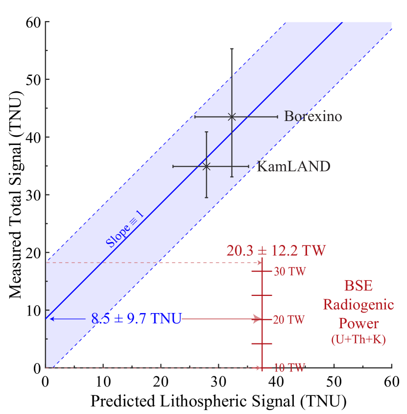
The measured signal at Borexino < TNU;¿agostini2015 and KamLAND < TNU;¿[]watanabe2016 are plotted against the predicted lithospheric signal from LITHO1.0 in Figure 5 in order to interpret the observed signals for BSE radiogenic power. Figure 5 represents a two-component system whereby the total measured signal (from the BSE) is comprised of the lithospheric and mantle signals. The slope is therefore defined equal to unity (i.e., y = x + b). The y-intercept, which represents the signal from the mantle, is calculated using Monte Carlo methods in order to account for asymmetric X and Y uncertainties. The predicted lithospheric signal for KamLAND and Borexino are correlated during the y-intercept Monte Carlo as most parameters are correlated within the geoneutrino reference model. Conversion of mantle TNU signal to BSE radiogenic power uses the relationship derived using the geoneutrino prediction model (similar to Figure 1 which shows total geoneutrino signal vs. radiogenic power in BSE). The estimated BSE radiogenic heat production of TW is consistent within 1-sigma of the low, medium, and high-H BSE models with the central value coincident with the medium-H model ( TW). Furthermore, the prediction given here using LITHO1.0 is consistent with that predicted by the \citeAsramek2016 model ( TW) when using the updated \citeAwatanabe2016 KamLAND measurement (personal communication). Based on Figure 5, an observed mantle signal of 8.5 TNU with uncertainty below some TNU is needed to discriminate between the different BSE compositional models. This uncertainty corresponds to a 40% reduction in the measured total and predicted lithospheric signal uncertainty at KamLAND and Borexino.
6.2 HPE Abundance and Heat Production
Abundances described in Table 2 for all layers are comparable (within 1) to both \citeArudnick2014 and \citeAhuang2013. However, uncertainties reported in the middle and lower crust are larger than those reported by \citeAhuang2013, likely due to differences in how these values were correlated. K/U and Th/U of the layers of the crust and bulk crust are also in agreement at 1 with previous estimates Huang \BOthers. (\APACyear2013); Rudnick \BBA Gao (\APACyear2014); Wipperfurth \BOthers. (\APACyear2018).
The bulk-continental crust heat production is negligibly different between the geophysical models (Table 2) and is consistent with previous estimates Mareschal \BBA Jaupart (\APACyear2013); Huang \BOthers. (\APACyear2014); Rudnick \BBA Gao (\APACyear2014). Furthermore, an estimate of bulk continental heat production of 7.0 TW (using LITHO1.0) encompasses average heat production in stable Precambrian (5.9 0.6 TW) and Phanerozoic (8.3 1.0 TW) crust estimated from heat flow studies Mareschal \BBA Jaupart (\APACyear2013). The similarity of continental crust heat production when using CRUST2.0 and LITHO1.0 is in contrast with the crustal signal similarity of CRUST1.0 and LITHO1.0 (Table 4) or the apparent crustal mass similarity of CRUST2.0 and CRUST1.0 observed in Figure 3 panel C. The similarity in crustal heat production of CRUST2.0 and LITHO1.0 is simply a reflection of their similar bulk crustal mass compared to the lower mass of CRUST1.0 (Table 1).
6.3 Uncertainties
The reported uncertainties for crustal abundances of the HPE in Table 2 are larger than that reported in \citeAhuang2013, primarily as a result of increased correlation of abundances and geophysical uncertainties. Increased correlation causes an inverse effect on uncertainty for the bulk crustal K/U and Th/U, resulting in less uncertainty than described by \citeAhuang2013. Some previous geoneutrino signal predictions did not include uncertainty on geophysical inputs, including crustal thickness <e.g.,¿enomoto2007,fiorentini2012,sramek2016, meaning these studies report smaller uncertainty on the geoneutrino signal. Similar to signal, the uncertainty on continental crustal heat production is 50% larger than that estimated by \citeAhuang2013 ( TW). In general, geophysical uncertainties (on thickness, density, and ) account for of the signal uncertainty, with the remaining proportion () from the geochemical inputs. When only considering the geophysical uncertainty, as the same geochemical method was applied to each geophysical model, the calculated crustal signals are still negligibly different.
7 Future Developments
The results from this study highlight the convergence of our understanding of the physical nature of the continental crust and the negligible effect of geophysical model on the predicted geoneutrino signal. Due to the strong effect of geochemical variability and distance from the detector on the predicted geoneutrino signal, future geoneutrino modeling needs to focus on better understanding of geochemical variability and a focus on near-field modeling. Below we highlight a few areas which require further exploration in order to better understand the crustal component of the geoneutrino signal.
7.1 Upper Crust Geochemical Uncertainty
The attribution of uncertainty on the concentration of heat producing elements in the upper crust (sigma-mean) in most geoneutrino studies (including this one) is not consistent with uncertainty on other parameters (1-sigma), including abundances in other layers. Often cited studies on the upper crust composition report sigma-mean Rudnick \BBA Gao (\APACyear2014) or Median Absolute Deviation <MAD;¿[]gaschnig2016, both of which report smaller error estimates than the standard deviation. Any regional or global geoneutrino modeling should adopt consistent error estimators, be it standard deviation or MAD, or justify the treatment of the upper crust separately from other portions of the crust. Upper crust U abundance used in this study is 2.7 0.6 (sigma-mean) from \citeArudnick2014, similar to that from \citeAgaschnig2016 of 2.66 0.87 . The standard deviation of the glacial diamictite data (assumed to sample large portions of the upper crust) from \citeAgaschnig2016 is 150% of the MAD. Because the upper crust is the dominant heat and geoneutrino emitter, consistent uncertainty estimates on abundances could significantly increase uncertainties on the predicted crustal geoneutrino signal. For example, attribution of abundances in the upper crust using 1-sigma values from a log-normal fit of \citeAgaschnig2016 data yields a total signal at KamLAND of 36.4 TNU (compared to 37.9 TNU reported in Table 4) using LITHO1.0. Use of 1-sigma uncertainty for the upper crust abundances therefore results in an increase of uncertainty of 40% in the predicted signal, an observation consistent with other studies <e.g.,¿takeuchi2019.
7.2 and Density under Himilayas and Andes
Future studies with the goal to update LITHO1.0 should aim to better understand the density and seismic structure beneath the Himalayas and Andes regions. The ’CRUST’ family of models predicts felsic-like densities in the entire crustal column in these regions (including the expected mafic lower crust; Figure 3). This prediction is in conflict with some regional studies <e.g.,¿monsalve2008,bai2013 although in agreement with other global studies <e.g.,¿hacker2015 and regional seismic models Agius \BBA Lebedev (\APACyear2017); Gilligan \BBA Priestley (\APACyear2018). Additionally, \citeApasyanos2014 perturbed CRUST1.0 parameters up to 5% to fit observed surface waves to make LITHO1.0, which a comparison of CRUST1.0 and LITHO1.0 in the Himilayan region shows that this perturbation reached saturation (i.e. 5% change between LITHO1.0 and CRUST1.0). If the model was not limited to 5% change the output would be more felsic than current. Because of the saturation of the method used by \citeApasyanos2014, LITHO1.0 in its current state may not be in agreement with observed regional data and should be revisited. Similar phenomena are observed under the Andes Mountains in South America <e.g.,¿lucassen2001. The Himilayas are particularly relevant for the geoneutrino prediction signal at Jinping and to a lesser extent, JUNO, while the Andes will be relevant to the future ANDES underground laboratory Bertou (\APACyear2012).
7.3 Geochemical Method for Middle and Lower Crust
The geochemical method of conversion of to [U,Th,K] does not work well in the lower crust (and to some degree in the middle crust) as the model often surpasses the endmember condition. This is a problem due to simplifying assumptions (i.e. assuming endmembers) indicating a need for a more sophisticated modeling space. A bivariate probability analysis of the available amphibolite or granulite samples with measured could avoid this problem (see Supporting Information for details). This analysis would not assume any specific relationship between and (unlike the linear relationship we assumed in this study) but instead would use the bivariate probability of and from the dataset. Currently there are too few samples (100–150) with measured to create a robust analysis. Incorporation of a thermodynamic modeling software <such as Perple_X;¿connolly2005) would allow for the calculation of seismic wavespeed for 500 samples, which would significantly increase the robustness of a bivariate probability analysis. Calculated using Perple_X for samples used in \citeAhuang2013 by \citeAhacker2015 closely resemble laboratory measurements, indicating the viability of thermodynamically calculated .
7.4 Near-field (regional) Modeling
Underestimation of the upper crust uncertainty or problems associated with middle/lower crust abundance calculations have less of an effect on predicted signals if a high-resolution regional geoneutrino model is combined with the global model <e.g.,¿enomoto2007,coltorti2011,huang2014,strati2017. Because of the distance dependence of the geoneutrino signal (see eq. 4) the regional area provides 40% of the geoneutrino signal at a detector as calculated in this study. High-resolution seismic and geochemical studies of the near-field therefore provide the most robust estimate of the signal at any detector location. This is exemplified in the studies of \citeAhuang2014 and \citeAstrati2017, who calculated larger uncertainties on the geoneutrino signal at SNO+ when they included a regional model compared to only using a global model. Although the uncertainty is larger than that estimated from the global model, their estimate includes more local information and is therefore likely to be a more accurate estimate of uncertainty.
Finally, evolution of our understanding of the physical and chemical nature of the bulk-crust is largely plateauing. This study showed that geoneutrino estimates using LITHO1.0 (2015), CRUST1.0 (2013), and CRUST2.0 (2001) yielded largely the same geoneutrino signal. Furthermore, the geochemical description of the crust from this study is consistent with the estimates by \citeArudnick2014, among others, which is itself consistent with \citeArudnick2003. Because of the natural variability of [U, Th, K] in the crust the uncertainty on bulk abundances is unlikely to change significantly. Joint inversions of multiple datasets, including teleseismic and , surface waves, gravity, surface heat flow, and topography/geoid have the most potential for significant advances in our understanding of the structure and composition of the crust (e.g., \citeAafonso2016,afonso2019). Regardless, improving our understanding of the physical and chemical nature of the bulk-crust will not have the same impact on reduction in the geoneutrino signal uncertainty as improvements in the near-field. As highlighted by \citeAstrati2017, better understanding of the physical structure with depth is the most difficult hurdle to overcome in near-field modeling.
8 Author Contributions
S.A.W. modeled the geoneutrino signal and wrote the text, with significant input on model creation, data analysis, and the text from O.Š. and W.F.M.
Acknowledgements.
Model results and original MATLAB code is provided in the Supporting Material. Support for this study was provided by the University of Maryland Graduate School ALL-S.T.A.R. Fellowship and NSF EAPSI program Award #1713230 (to S.A.W), NSF grant EAR1650365 (to W.F.M.), and the Czech Science Foundation grant GAČR 17-01464S (to O.Š.). There are no financial or interest conflicts with this work. We thank Fabio Mantovani, Bedřich Roskovec, and Steve Dye for insightful comments and discussion.References
- Afonso \BOthers. (\APACyear2016) \APACinsertmetastarafonso2016{APACrefauthors}Afonso, J\BPBIC., Rawlinson, N., Yang, Y., Schutt, D\BPBIL., Jones, A\BPBIG., Fullea, J.\BCBL \BBA Griffin, W\BPBIL. \APACrefYearMonthDay2016. \BBOQ\APACrefatitle3-D Multiobservable Probabilistic Inversion for the Compositional and Thermal Structure of the Lithosphere and Upper Mantle: III. Thermochemical Tomography in the Western-Central U.S. 3-D multiobservable probabilistic inversion for the compositional and thermal structure of the lithosphere and upper mantle: III. Thermochemical tomography in the Western-Central U.S.\BBCQ \APACjournalVolNumPagesJournal of Geophysical Research: Solid Earth121102016JB013049. {APACrefDOI} 10.1002/2016JB013049 \PrintBackRefs\CurrentBib
- Afonso \BOthers. (\APACyear2019) \APACinsertmetastarafonso2019{APACrefauthors}Afonso, J\BPBIC., Salajegheh, F., Szwillus, W., Ebbing, J.\BCBL \BBA Gaina, C. \APACrefYearMonthDay2019. \BBOQ\APACrefatitleA Global Reference Model of the Lithosphere and Upper Mantle from Joint Inversion and Analysis of Multiple Data Sets A global reference model of the lithosphere and upper mantle from joint inversion and analysis of multiple data sets.\BBCQ \APACjournalVolNumPagesGeophysical Journal International21731602-1628. {APACrefDOI} 10.1093/gji/ggz094 \PrintBackRefs\CurrentBib
- Agius \BBA Lebedev (\APACyear2017) \APACinsertmetastaragius2017{APACrefauthors}Agius, M\BPBIR.\BCBT \BBA Lebedev, S. \APACrefYearMonthDay2017. \BBOQ\APACrefatitleComplex, Multilayered Azimuthal Anisotropy beneath Tibet: Evidence for Co-Existing Channel Flow and Pure-Shear Crustal Thickening Complex, multilayered azimuthal anisotropy beneath Tibet: Evidence for co-existing channel flow and pure-shear crustal thickening.\BBCQ \APACjournalVolNumPagesGeophysical Journal International21031823-1844. {APACrefDOI} 10.1093/gji/ggx266 \PrintBackRefs\CurrentBib
- Agostini \BOthers. (\APACyear2015) \APACinsertmetastaragostini2015{APACrefauthors}Agostini, M., Appel, S., Bellini, G., Benziger, J., Bick, D., Bonfini, G.\BDBLothers \APACrefYearMonthDay2015. \BBOQ\APACrefatitleSpectroscopy of Geoneutrinos from 2056 Days of Borexino Data Spectroscopy of geoneutrinos from 2056 days of Borexino data.\BBCQ \APACjournalVolNumPagesPhysical Review D923031101. {APACrefDOI} https://doi.org/10.1103/PhysRevD.92.031101 \PrintBackRefs\CurrentBib
- Ahrens (\APACyear1954) \APACinsertmetastarahrens1954{APACrefauthors}Ahrens, L\BPBIH. \APACrefYearMonthDay1954. \BBOQ\APACrefatitleThe Lognormal Distribution of the Elements (A Fundamental Law of Geochemistry and Its Subsidiary) The lognormal distribution of the elements (A fundamental law of geochemistry and its subsidiary).\BBCQ \APACjournalVolNumPagesGeochimica et Cosmochimica Acta5249-73. {APACrefDOI} 10.1016/0016-7037(54)90040-X \PrintBackRefs\CurrentBib
- Araki \BOthers. (\APACyear2005) \APACinsertmetastararaki2005{APACrefauthors}Araki, T., Enomoto, S., Furuno, K., Gando, Y., Ichimura, K., Ikeda, H.\BDBLPiquemal, F. \APACrefYearMonthDay2005. \BBOQ\APACrefatitleExperimental Investigation of Geologically Produced Antineutrinos with KamLAND Experimental investigation of geologically produced antineutrinos with KamLAND.\BBCQ \APACjournalVolNumPagesNature4367050499-503. {APACrefDOI} 10.1038/nature03980 \PrintBackRefs\CurrentBib
- Arevalo \BOthers. (\APACyear2009) \APACinsertmetastararevalo2009{APACrefauthors}Arevalo, R., McDonough, W\BPBIF.\BCBL \BBA Luong, M. \APACrefYearMonthDay2009. \BBOQ\APACrefatitleThe K/U Ratio of the Silicate Earth: Insights into Mantle Composition, Structure and Thermal Evolution The K/U ratio of the silicate Earth: Insights into mantle composition, structure and thermal evolution.\BBCQ \APACjournalVolNumPagesEarth and Planetary Science Letters2783-4361-369. {APACrefDOI} 10.1016/j.epsl.2008.12.023 \PrintBackRefs\CurrentBib
- Arevalo \BOthers. (\APACyear2013) \APACinsertmetastararevalo2013{APACrefauthors}Arevalo, R., McDonough, W\BPBIF., Stracke, A., Willbold, M., Ireland, T\BPBIJ.\BCBL \BBA Walker, R\BPBIJ. \APACrefYearMonthDay2013. \BBOQ\APACrefatitleSimplified Mantle Architecture and Distribution of Radiogenic Power Simplified mantle architecture and distribution of radiogenic power.\BBCQ \APACjournalVolNumPagesGeochemistry, Geophysics, Geosystems1472265-2285. {APACrefDOI} 10.1002/ggge.20152 \PrintBackRefs\CurrentBib
- Bai \BOthers. (\APACyear2013) \APACinsertmetastarbai2013{APACrefauthors}Bai, Z., Zhang, S.\BCBL \BBA Braitenberg, C. \APACrefYearMonthDay2013. \BBOQ\APACrefatitleCrustal Density Structure from 3D Gravity Modeling beneath Himalaya and Lhasa Blocks, Tibet Crustal density structure from 3D gravity modeling beneath Himalaya and Lhasa blocks, Tibet.\BBCQ \APACjournalVolNumPagesJournal of Asian Earth Sciences78301-317. {APACrefDOI} 10.1016/j.jseaes.2012.12.035 \PrintBackRefs\CurrentBib
- Bassin \BOthers. (\APACyear2000) \APACinsertmetastarbassin2000{APACrefauthors}Bassin, C., Laske, G.\BCBL \BBA Masters, T\BPBIG. \APACrefYearMonthDay2000. \BBOQ\APACrefatitleThe Current Limits of Resolution for Surface Wave Tomography in North America The current limits of resolution for surface wave tomography in North America.\BBCQ \APACjournalVolNumPagesEos Trans. AGU. \PrintBackRefs\CurrentBib
- Bertou (\APACyear2012) \APACinsertmetastarbertou2012{APACrefauthors}Bertou, X. \APACrefYearMonthDay2012. \BBOQ\APACrefatitleThe ANDES Underground Laboratory The ANDES underground laboratory.\BBCQ \APACjournalVolNumPagesThe European Physical Journal Plus1279104. {APACrefDOI} 10.1140/epjp/i2012-12104-1 \PrintBackRefs\CurrentBib
- Capozzi \BOthers. (\APACyear2017) \APACinsertmetastarcapozzi2017{APACrefauthors}Capozzi, F., Di Valentino, E., Lisi, E., Marrone, A., Melchiorri, A.\BCBL \BBA Palazzo, A. \APACrefYearMonthDay2017. \BBOQ\APACrefatitleGlobal Constraints on Absolute Neutrino Masses and Their Ordering Global constraints on absolute neutrino masses and their ordering.\BBCQ \APACjournalVolNumPagesPhysical Review D959096014. {APACrefDOI} 10.1103/PhysRevD.95.096014 \PrintBackRefs\CurrentBib
- Christensen (\APACyear1965) \APACinsertmetastarchristensen1965{APACrefauthors}Christensen, N\BPBII. \APACrefYearMonthDay1965. \BBOQ\APACrefatitleCompressional Wave Velocities in Metamorphic Rocks at Pressures to 10 Kilobars Compressional wave velocities in metamorphic rocks at pressures to 10 kilobars.\BBCQ \APACjournalVolNumPagesJournal of Geophysical Research70246147-6164. {APACrefDOI} 10.1029/JZ070i024p06147 \PrintBackRefs\CurrentBib
- Christensen \BBA Mooney (\APACyear1995) \APACinsertmetastarchristensen1995{APACrefauthors}Christensen, N\BPBII.\BCBT \BBA Mooney, W\BPBID. \APACrefYearMonthDay1995. \BBOQ\APACrefatitleSeismic Velocity Structure and Composition of the Continental Crust: A Global View Seismic velocity structure and composition of the continental crust: A global view.\BBCQ \APACjournalVolNumPagesJournal of Geophysical Research: Solid Earth100B69761-9788. {APACrefDOI} 10.1029/95JB00259 \PrintBackRefs\CurrentBib
- Coltorti \BOthers. (\APACyear2011) \APACinsertmetastarcoltorti2011{APACrefauthors}Coltorti, M., Boraso, R., Mantovani, F., Morsilli, M., Fiorentini, G., Riva, A.\BDBLChubakov, V. \APACrefYearMonthDay2011. \BBOQ\APACrefatitleU and Th Content in the Central Apennines Continental Crust: A Contribution to the Determination of the Geo-Neutrinos Flux at LNGS U and Th content in the Central Apennines continental crust: A contribution to the determination of the geo-neutrinos flux at LNGS.\BBCQ \APACjournalVolNumPagesGeochimica et Cosmochimica Acta7592271-2294. {APACrefDOI} 10.1016/j.gca.2011.01.024 \PrintBackRefs\CurrentBib
- Connolly (\APACyear2005) \APACinsertmetastarconnolly2005{APACrefauthors}Connolly, J\BPBIA\BPBID. \APACrefYearMonthDay2005. \BBOQ\APACrefatitleComputation of Phase Equilibria by Linear Programming: A Tool for Geodynamic Modeling and Its Application to Subduction Zone Decarbonation Computation of phase equilibria by linear programming: A tool for geodynamic modeling and its application to subduction zone decarbonation.\BBCQ \APACjournalVolNumPagesEarth and Planetary Science Letters2361524-541. {APACrefDOI} 10.1016/j.epsl.2005.04.033 \PrintBackRefs\CurrentBib
- G\BPBIF. Davies (\APACyear1980) \APACinsertmetastardavies1980{APACrefauthors}Davies, G\BPBIF. \APACrefYearMonthDay1980. \BBOQ\APACrefatitleThermal Histories of Convective Earth Models and Constraints on Radiogenic Heat Production in the Earth Thermal histories of convective Earth models and constraints on radiogenic heat production in the Earth.\BBCQ \APACjournalVolNumPagesJournal of Geophysical Research: Solid Earth85B52517-2530. {APACrefDOI} 10.1029/JB085iB05p02517 \PrintBackRefs\CurrentBib
- J\BPBIH. Davies \BBA Davies (\APACyear2010) \APACinsertmetastardavies2010{APACrefauthors}Davies, J\BPBIH.\BCBT \BBA Davies, D\BPBIR. \APACrefYearMonthDay2010. \BBOQ\APACrefatitleEarth’s Surface Heat Flux Earth’s surface heat flux.\BBCQ \APACjournalVolNumPagesSolid Earth115-24. {APACrefDOI} 10.5194/se-1-5-2010 \PrintBackRefs\CurrentBib
- Dye (\APACyear2012) \APACinsertmetastardye2012{APACrefauthors}Dye, S\BPBIT. \APACrefYearMonthDay2012. \BBOQ\APACrefatitleGeoneutrinos and the Radioactive Power of the Earth Geoneutrinos and the radioactive power of the Earth.\BBCQ \APACjournalVolNumPagesReviews of Geophysics503. {APACrefDOI} 10.1029/2012RG000400 \PrintBackRefs\CurrentBib
- Dziewonski \BBA Anderson (\APACyear1981) \APACinsertmetastardziewonski1981{APACrefauthors}Dziewonski, A\BPBIM.\BCBT \BBA Anderson, D\BPBIL. \APACrefYearMonthDay1981. \BBOQ\APACrefatitlePreliminary Reference Earth Model Preliminary reference Earth model.\BBCQ \APACjournalVolNumPagesPhysics of the Earth and Planetary Interiors254297-356. {APACrefDOI} 10.1016/0031-9201(81)90046-7 \PrintBackRefs\CurrentBib
- Enomoto (\APACyear2006) \APACinsertmetastarenomoto:nuspec{APACrefauthors}Enomoto, S. \APACrefYearMonthDay2006. \APACrefbtitleGeoneutrino Spectrum and Luminosity. Geoneutrino spectrum and luminosity. {APACrefURL} [2006]http://www.awa.tohoku.ac.jp/~sanshiro/research/geoneutrino/spectrum/ \PrintBackRefs\CurrentBib
- Enomoto \BOthers. (\APACyear2007) \APACinsertmetastarenomoto2007{APACrefauthors}Enomoto, S., Ohtani, E., Inoue, K.\BCBL \BBA Suzuki, A. \APACrefYearMonthDay2007. \BBOQ\APACrefatitleNeutrino Geophysics with KamLAND and Future Prospects Neutrino geophysics with KamLAND and future prospects.\BBCQ \APACjournalVolNumPagesEarth and Planetary Science Letters2581-2147-159. {APACrefDOI} 10.1016/j.epsl.2007.03.038 \PrintBackRefs\CurrentBib
- Fiorentini \BOthers. (\APACyear2012) \APACinsertmetastarfiorentini2012{APACrefauthors}Fiorentini, G., Fogli, G\BPBIL., Lisi, E., Mantovani, F.\BCBL \BBA Rotunno, A\BPBIM. \APACrefYearMonthDay2012. \BBOQ\APACrefatitleMantle Geoneutrinos in KamLAND and Borexino Mantle geoneutrinos in KamLAND and Borexino.\BBCQ \APACjournalVolNumPagesPhysical Review D863. {APACrefDOI} 10.1103/PhysRevD.86.033004 \PrintBackRefs\CurrentBib
- Gaschnig \BOthers. (\APACyear2016) \APACinsertmetastargaschnig2016{APACrefauthors}Gaschnig, R\BPBIM., Rudnick, R\BPBIL., McDonough, W\BPBIF., Kaufman, A\BPBIJ., Valley, J\BPBIW., Hu, Z.\BDBLBeck, M\BPBIL. \APACrefYearMonthDay2016. \BBOQ\APACrefatitleCompositional Evolution of the Upper Continental Crust through Time, as Constrained by Ancient Glacial Diamictites Compositional evolution of the upper continental crust through time, as constrained by ancient glacial diamictites.\BBCQ \APACjournalVolNumPagesGeochimica et Cosmochimica Acta186316-343. {APACrefDOI} 10.1016/j.gca.2016.03.020 \PrintBackRefs\CurrentBib
- Gilligan \BBA Priestley (\APACyear2018) \APACinsertmetastargilligan2018{APACrefauthors}Gilligan, A.\BCBT \BBA Priestley, K. \APACrefYearMonthDay2018. \BBOQ\APACrefatitleLateral Variations in the Crustal Structure of the Indo–Eurasian Collision Zone Lateral variations in the crustal structure of the Indo–Eurasian collision zone.\BBCQ \APACjournalVolNumPagesGeophysical Journal International2142975-989. {APACrefDOI} 10.1093/gji/ggy172 \PrintBackRefs\CurrentBib
- Hacker \BOthers. (\APACyear2015) \APACinsertmetastarhacker2015{APACrefauthors}Hacker, B\BPBIR., Kelemen, P\BPBIB.\BCBL \BBA Behn, M\BPBID. \APACrefYearMonthDay2015. \BBOQ\APACrefatitleContinental Lower Crust Continental Lower Crust.\BBCQ \APACjournalVolNumPagesAnnual Review of Earth and Planetary Sciences431167-205. {APACrefDOI} 10.1146/annurev-earth-050212-124117 \PrintBackRefs\CurrentBib
- Huang \BOthers. (\APACyear2013) \APACinsertmetastarhuang2013{APACrefauthors}Huang, Y., Chubakov, V., Mantovani, F., Rudnick, R\BPBIL.\BCBL \BBA McDonough, W\BPBIF. \APACrefYearMonthDay2013. \BBOQ\APACrefatitleA Reference Earth Model for the Heat-Producing Elements and Associated Geoneutrino Flux A reference Earth model for the heat-producing elements and associated geoneutrino flux.\BBCQ \APACjournalVolNumPagesGeochemistry, Geophysics, Geosystems1462003-2029. {APACrefDOI} 10.1002/ggge.20129 \PrintBackRefs\CurrentBib
- Huang \BOthers. (\APACyear2014) \APACinsertmetastarhuang2014{APACrefauthors}Huang, Y., Strati, V., Mantovani, F., Shirey, S\BPBIB.\BCBL \BBA McDonough, W\BPBIF. \APACrefYearMonthDay2014. \BBOQ\APACrefatitleRegional Study of the Archean to Proterozoic Crust at the Sudbury Neutrino Observatory (SNO+), Ontario: Predicting the Geoneutrino Flux Regional study of the Archean to Proterozoic crust at the Sudbury Neutrino Observatory (SNO+), Ontario: Predicting the geoneutrino flux.\BBCQ \APACjournalVolNumPagesGeochemistry, Geophysics, Geosystems15103925-3944. {APACrefDOI} 10.1002/2014GC005397 \PrintBackRefs\CurrentBib
- Inman \BBA Bradley Jr. (\APACyear1989) \APACinsertmetastarinman1989{APACrefauthors}Inman, H\BPBIF.\BCBT \BBA Bradley Jr., E\BPBIL. \APACrefYearMonthDay1989. \BBOQ\APACrefatitleThe Overlapping Coefficient as a Measure of Agreement between Probability Distributions and Point Estimation of the Overlap of Two Normal Densities The overlapping coefficient as a measure of agreement between probability distributions and point estimation of the overlap of two normal densities.\BBCQ \APACjournalVolNumPagesCommunications in Statistics - Theory and Methods18103851-3874. {APACrefDOI} 10.1080/03610928908830127 \PrintBackRefs\CurrentBib
- Javoy (\APACyear1999) \APACinsertmetastarjavoy1999{APACrefauthors}Javoy, M. \APACrefYearMonthDay1999. \BBOQ\APACrefatitleChemical Earth Models Chemical earth models.\BBCQ \APACjournalVolNumPagesComptes Rendus de l’Académie des Sciences - Series IIA - Earth and Planetary Science3298537-555. {APACrefDOI} 10.1016/S1251-8050(00)87210-9 \PrintBackRefs\CurrentBib
- Javoy \BOthers. (\APACyear2010) \APACinsertmetastarjavoy2010{APACrefauthors}Javoy, M., Kaminski, E., Guyot, F., Andrault, D., Sanloup, C., Moreira, M.\BDBLJaupart, C. \APACrefYearMonthDay2010. \BBOQ\APACrefatitleThe Chemical Composition of the Earth: Enstatite Chondrite Models The chemical composition of the Earth: Enstatite chondrite models.\BBCQ \APACjournalVolNumPagesEarth and Planetary Science Letters2933-4259-268. {APACrefDOI} 10.1016/j.epsl.2010.02.033 \PrintBackRefs\CurrentBib
- Laske \BOthers. (\APACyear2013) \APACinsertmetastarlaske2013{APACrefauthors}Laske, G., Masters, G., Ma, Z.\BCBL \BBA Pasyanos, M\BPBIE. \APACrefYearMonthDay2013. \BBOQ\APACrefatitleUpdate on CRUST1.0 - A 1-Degree Global Model of Earth’s Crust Update on CRUST1.0 - A 1-degree Global Model of Earth’s Crust.\BBCQ \BIn \APACrefbtitleGeophysical Research Abstracts Geophysical Research Abstracts (\BVOL 15). \PrintBackRefs\CurrentBib
- Laske \BBA Masters (\APACyear1997) \APACinsertmetastarlaske1997{APACrefauthors}Laske, G.\BCBT \BBA Masters, T\BPBIG. \APACrefYearMonthDay1997. \BBOQ\APACrefatitleA Global Digital Map of Sediment Thickness A global digital map of sediment thickness.\BBCQ \APACjournalVolNumPagesEOS Trans. AGU78F483. \PrintBackRefs\CurrentBib
- Lucassen \BOthers. (\APACyear2001) \APACinsertmetastarlucassen2001{APACrefauthors}Lucassen, F., Becchio, R., Harmon, R., Kasemann, S., Franz, G., Trumbull, R.\BDBLDulski, P. \APACrefYearMonthDay2001. \BBOQ\APACrefatitleComposition and Density Model of the Continental Crust at an Active Continental Margin—the Central Andes between 21° and 27°S Composition and density model of the continental crust at an active continental margin—the Central Andes between 21° and 27°S.\BBCQ \APACjournalVolNumPagesTectonophysics3411195-223. {APACrefDOI} 10.1016/S0040-1951(01)00188-3 \PrintBackRefs\CurrentBib
- Mantovani \BOthers. (\APACyear2004) \APACinsertmetastarmantovani2004{APACrefauthors}Mantovani, F., Carmignani, L., Fiorentini, G.\BCBL \BBA Lissia, M. \APACrefYearMonthDay2004. \BBOQ\APACrefatitleAntineutrinos from Earth: A Reference Model and Its Uncertainties Antineutrinos from Earth: A reference model and its uncertainties.\BBCQ \APACjournalVolNumPagesPhysical Review D691. {APACrefDOI} 10.1103/PhysRevD.69.013001 \PrintBackRefs\CurrentBib
- Mareschal \BBA Jaupart (\APACyear2013) \APACinsertmetastarmareschal2013{APACrefauthors}Mareschal, J\BHBIC.\BCBT \BBA Jaupart, C. \APACrefYearMonthDay2013. \BBOQ\APACrefatitleRadiogenic Heat Production, Thermal Regime and Evolution of Continental Crust Radiogenic heat production, thermal regime and evolution of continental crust.\BBCQ \APACjournalVolNumPagesTectonophysics609524-534. {APACrefDOI} 10.1016/j.tecto.2012.12.001 \PrintBackRefs\CurrentBib
- McDonough (\APACyear1990) \APACinsertmetastarmcdonough1990{APACrefauthors}McDonough, W\BPBIF. \APACrefYearMonthDay1990. \BBOQ\APACrefatitleConstraints on the Composition of the Continental Lithospheric Mantle Constraints on the composition of the continental lithospheric mantle.\BBCQ \APACjournalVolNumPagesEarth and Planetary Science Letters10111-18. {APACrefDOI} 10.1016/0012-821X(90)90119-I \PrintBackRefs\CurrentBib
- McDonough (\APACyear2017) \APACinsertmetastarmcdonough2017{APACrefauthors}McDonough, W\BPBIF. \APACrefYearMonthDay2017. \BBOQ\APACrefatitleEarth’s Core Earth’s Core.\BBCQ \BIn W\BPBIM. White (\BED), \APACrefbtitleEncyclopedia of Geochemistry Encyclopedia of Geochemistry (\BPG 1-13). \APACaddressPublisherSpringer International Publishing. {APACrefDOI} 10.1007/978-3-319-39193-9_258-1 \PrintBackRefs\CurrentBib
- McDonough \BBA Sun (\APACyear1995) \APACinsertmetastarmcdonough1995{APACrefauthors}McDonough, W\BPBIF.\BCBT \BBA Sun, S\BHBIs. \APACrefYearMonthDay1995. \BBOQ\APACrefatitleThe Composition of the Earth The composition of the Earth.\BBCQ \APACjournalVolNumPagesChemical Geology1203-4223-253. {APACrefDOI} 10.1016/0009-2541(94)00140-4 \PrintBackRefs\CurrentBib
- Monsalve \BOthers. (\APACyear2008) \APACinsertmetastarmonsalve2008{APACrefauthors}Monsalve, G., Sheehan, A., Rowe, C.\BCBL \BBA Rajaure, S. \APACrefYearMonthDay2008. \BBOQ\APACrefatitleSeismic Structure of the Crust and the Upper Mantle beneath the Himalayas: Evidence for Eclogitization of Lower Crustal Rocks in the Indian Plate Seismic structure of the crust and the upper mantle beneath the Himalayas: Evidence for eclogitization of lower crustal rocks in the Indian Plate.\BBCQ \APACjournalVolNumPagesJournal of Geophysical Research: Solid Earth113B8. {APACrefDOI} 10.1029/2007JB005424 \PrintBackRefs\CurrentBib
- Mooney \BOthers. (\APACyear1998) \APACinsertmetastarmooney1998{APACrefauthors}Mooney, W\BPBID., Laske, G.\BCBL \BBA Masters, T\BPBIG. \APACrefYearMonthDay1998. \BBOQ\APACrefatitleCRUST 5.1: A Global Crustal Model at 5° × 5° CRUST 5.1: A global crustal model at 5° × 5°.\BBCQ \APACjournalVolNumPagesJournal of Geophysical Research: Solid Earth103B1727-747. {APACrefDOI} 10.1029/97JB02122 \PrintBackRefs\CurrentBib
- Olugboji \BOthers. (\APACyear2017) \APACinsertmetastarolugboji2017{APACrefauthors}Olugboji, T\BPBIM., Lekic, V.\BCBL \BBA McDonough, W\BPBIF. \APACrefYearMonthDay2017. \BBOQ\APACrefatitleA Statistical Assessment of Seismic Models of the U.S. Continental Crust Using Bayesian Inversion of Ambient Noise Surface Wave Dispersion Data A statistical assessment of seismic models of the U.S. continental crust using Bayesian inversion of ambient noise surface wave dispersion data.\BBCQ \APACjournalVolNumPagesTectonics2017TC004468. {APACrefDOI} 10.1002/2017TC004468 \PrintBackRefs\CurrentBib
- O’Neill \BBA Palme (\APACyear2008) \APACinsertmetastaroneill2008{APACrefauthors}O’Neill, H\BPBIS.\BCBT \BBA Palme, H. \APACrefYearMonthDay2008. \BBOQ\APACrefatitleCollisional Erosion and the Non-Chondritic Composition of the Terrestrial Planets Collisional erosion and the non-chondritic composition of the terrestrial planets.\BBCQ \APACjournalVolNumPagesPhilosophical Transactions of the Royal Society A: Mathematical, Physical and Engineering Sciences36618834205-4238. {APACrefDOI} 10.1098/rsta.2008.0111 \PrintBackRefs\CurrentBib
- Pakiser \BBA Robinson (\APACyear1966) \APACinsertmetastarpakiser1966{APACrefauthors}Pakiser, L\BPBIC.\BCBT \BBA Robinson, R. \APACrefYearMonthDay1966. \BBOQ\APACrefatitleComposition and Evolution of the Continental Crust as Suggested by Seismic Observations Composition and evolution of the continental crust as suggested by seismic observations.\BBCQ \APACjournalVolNumPagesTectonophysics36547-557. {APACrefDOI} 10.1016/0040-1951(66)90030-8 \PrintBackRefs\CurrentBib
- Palme \BBA O’Neill (\APACyear2014) \APACinsertmetastarpalme2014{APACrefauthors}Palme, H.\BCBT \BBA O’Neill, H. \APACrefYearMonthDay2014. \BBOQ\APACrefatitleCosmochemical Estimates of Mantle Composition Cosmochemical Estimates of Mantle Composition.\BBCQ \BIn \APACrefbtitleTreatise on Geochemistry Treatise on Geochemistry (\BPG 1-39). \APACaddressPublisherElsevier. {APACrefDOI} 10.1016/B978-0-08-095975-7.00201-1 \PrintBackRefs\CurrentBib
- Pasyanos \BOthers. (\APACyear2014) \APACinsertmetastarpasyanos2014{APACrefauthors}Pasyanos, M\BPBIE., Masters, T\BPBIG., Laske, G.\BCBL \BBA Ma, Z. \APACrefYearMonthDay2014. \BBOQ\APACrefatitleLITHO1.0: An Updated Crust and Lithospheric Model of the Earth: LITHO1.0 LITHO1.0: An updated crust and lithospheric model of the Earth: LITHO1.0.\BBCQ \APACjournalVolNumPagesJournal of Geophysical Research: Solid Earth11932153-2173. {APACrefDOI} 10.1002/2013JB010626 \PrintBackRefs\CurrentBib
- Plank (\APACyear2014) \APACinsertmetastarplank2014{APACrefauthors}Plank, T. \APACrefYearMonthDay2014. \BBOQ\APACrefatitleThe Chemical Composition of Subducting Sediments The Chemical Composition of Subducting Sediments.\BBCQ \BIn \APACrefbtitleTreatise on Geochemistry Treatise on Geochemistry (\BPG 607-629). \APACaddressPublisherElsevier. {APACrefDOI} 10.1016/B978-0-08-095975-7.00319-3 \PrintBackRefs\CurrentBib
- Pollack \BBA Chapman (\APACyear1977) \APACinsertmetastarpollack1977{APACrefauthors}Pollack, H\BPBIN.\BCBT \BBA Chapman, D\BPBIS. \APACrefYearMonthDay1977. \BBOQ\APACrefatitleOn the Regional Variation of Heat Flow, Geotherms, and Lithospheric Thickness On the regional variation of heat flow, geotherms, and lithospheric thickness.\BBCQ \APACjournalVolNumPagesTectonophysics383279-296. {APACrefDOI} 10.1016/0040-1951(77)90215-3 \PrintBackRefs\CurrentBib
- Reguzzoni \BBA Sampietro (\APACyear2015) \APACinsertmetastarreguzzoni2015{APACrefauthors}Reguzzoni, M.\BCBT \BBA Sampietro, D. \APACrefYearMonthDay2015. \BBOQ\APACrefatitleGEMMA: An Earth Crustal Model Based on GOCE Satellite Data GEMMA: An Earth crustal model based on GOCE satellite data.\BBCQ \APACjournalVolNumPagesInternational Journal of Applied Earth Observation and Geoinformation3531-43. {APACrefDOI} 10.1016/j.jag.2014.04.002 \PrintBackRefs\CurrentBib
- Rudnick \BBA Fountain (\APACyear1995) \APACinsertmetastarrudnick1995{APACrefauthors}Rudnick, R\BPBIL.\BCBT \BBA Fountain, D\BPBIM. \APACrefYearMonthDay1995. \BBOQ\APACrefatitleNature and Composition of the Continental Crust: A Lower Crustal Perspective Nature and composition of the continental crust: A lower crustal perspective.\BBCQ \APACjournalVolNumPagesReviews of Geophysics333267. {APACrefDOI} 10.1029/95RG01302 \PrintBackRefs\CurrentBib
- Rudnick \BBA Gao (\APACyear2003) \APACinsertmetastarrudnick2003{APACrefauthors}Rudnick, R\BPBIL.\BCBT \BBA Gao, S. \APACrefYearMonthDay2003. \BBOQ\APACrefatitleComposition of the Continental Crust Composition of the Continental Crust.\BBCQ \BIn \APACrefbtitleTreatise on Geochemistry Treatise on Geochemistry (\BPG 1-64). \APACaddressPublisherElsevier. \PrintBackRefs\CurrentBib
- Rudnick \BBA Gao (\APACyear2014) \APACinsertmetastarrudnick2014{APACrefauthors}Rudnick, R\BPBIL.\BCBT \BBA Gao, S. \APACrefYearMonthDay2014. \BBOQ\APACrefatitleComposition of the Continental Crust Composition of the Continental Crust.\BBCQ \BIn \APACrefbtitleTreatise on Geochemistry Treatise on Geochemistry (\BPG 1-51). \APACaddressPublisherElsevier. {APACrefDOI} 10.1016/B978-0-08-095975-7.00301-6 \PrintBackRefs\CurrentBib
- Ruedas (\APACyear2017) \APACinsertmetastarruedas2017{APACrefauthors}Ruedas, T. \APACrefYearMonthDay2017. \BBOQ\APACrefatitleRadioactive Heat Production of Six Geologically Important Nuclides Radioactive heat production of six geologically important nuclides.\BBCQ \APACjournalVolNumPagesGeochemistry, Geophysics, Geosystems1893530-3541. {APACrefDOI} 10.1002/2017GC006997 \PrintBackRefs\CurrentBib
- Schubert \BOthers. (\APACyear1980) \APACinsertmetastarschubert1980{APACrefauthors}Schubert, G., Stevenson, D.\BCBL \BBA Cassen, P. \APACrefYearMonthDay1980. \BBOQ\APACrefatitleWhole Planet Cooling and the Radiogenic Heat Source Contents of the Earth and Moon Whole planet cooling and the radiogenic heat source contents of the Earth and Moon.\BBCQ \APACjournalVolNumPagesJournal of Geophysical Research: Solid Earth85B52531-2538. {APACrefDOI} 10.1029/JB085iB05p02531 \PrintBackRefs\CurrentBib
- Shapiro \BBA Ritzwoller (\APACyear2002) \APACinsertmetastarshapiro2002{APACrefauthors}Shapiro, N\BPBIM.\BCBT \BBA Ritzwoller, M\BPBIH. \APACrefYearMonthDay2002. \BBOQ\APACrefatitleMonte-Carlo Inversion for a Global Shear-Velocity Model of the Crust and Upper Mantle Monte-Carlo inversion for a global shear-velocity model of the crust and upper mantle.\BBCQ \APACjournalVolNumPagesGeophysical Journal International151188-105. {APACrefDOI} 10.1046/j.1365-246X.2002.01742.x \PrintBackRefs\CurrentBib
- Šrámek \BOthers. (\APACyear2016) \APACinsertmetastarsramek2016{APACrefauthors}Šrámek, O., Roskovec, B., Wipperfurth, S\BPBIA., Xi, Y.\BCBL \BBA McDonough, W\BPBIF. \APACrefYearMonthDay2016. \BBOQ\APACrefatitleRevealing the Earth’s Mantle from the Tallest Mountains Using the Jinping Neutrino Experiment Revealing the Earth’s mantle from the tallest mountains using the Jinping Neutrino Experiment.\BBCQ \APACjournalVolNumPagesScientific Reports633034. {APACrefDOI} 10.1038/srep33034 \PrintBackRefs\CurrentBib
- Steinberger \BBA Becker (\APACyear2016) \APACinsertmetastarsteinberger2016{APACrefauthors}Steinberger, B.\BCBT \BBA Becker, T\BPBIW. \APACrefYearMonthDay2016. \BBOQ\APACrefatitleA Comparison of Lithospheric Thickness Models A comparison of lithospheric thickness models.\BBCQ \APACjournalVolNumPagesTectonophysics. {APACrefDOI} 10.1016/j.tecto.2016.08.001 \PrintBackRefs\CurrentBib
- Strati \BOthers. (\APACyear2015) \APACinsertmetastarstrati2015{APACrefauthors}Strati, V., Baldoncini, M., Callegari, I., Mantovani, F., McDonough, W\BPBIF., Ricci, B.\BCBL \BBA Xhixha, G. \APACrefYearMonthDay2015. \BBOQ\APACrefatitleExpected Geoneutrino Signal at JUNO Expected geoneutrino signal at JUNO.\BBCQ \APACjournalVolNumPagesProgress in Earth and Planetary Science21. {APACrefDOI} 10.1186/s40645-015-0037-6 \PrintBackRefs\CurrentBib
- Strati \BOthers. (\APACyear2017) \APACinsertmetastarstrati2017{APACrefauthors}Strati, V., Wipperfurth, S\BPBIA., Baldoncini, M., McDonough, W\BPBIF.\BCBL \BBA Mantovani, F. \APACrefYearMonthDay2017. \BBOQ\APACrefatitlePerceiving the Crust in 3-D: A Model Integrating Geological, Geochemical, and Geophysical Data Perceiving the Crust in 3-D: A Model Integrating Geological, Geochemical, and Geophysical Data.\BBCQ \APACjournalVolNumPagesGeochemistry, Geophysics, Geosystems18124326-4341. {APACrefDOI} 10.1002/2017GC007067 \PrintBackRefs\CurrentBib
- Takeuchi \BOthers. (\APACyear2019) \APACinsertmetastartakeuchi2019{APACrefauthors}Takeuchi, N., Ueki, K., Iizuka, T., Nagao, J., Tanaka, A., Enomoto, S.\BDBLTanaka, H\BPBIK\BPBIM. \APACrefYearMonthDay2019. \BBOQ\APACrefatitleStochastic Modeling of 3-D Compositional Distribution in the Crust with Bayesian Inference and Application to Geoneutrino Observation in Japan Stochastic Modeling of 3-D Compositional Distribution in the Crust with Bayesian Inference and Application to Geoneutrino Observation in Japan.\BBCQ \APACjournalVolNumPagesPhysics of the Earth and Planetary Interiors. {APACrefDOI} 10.1016/j.pepi.2019.01.002 \PrintBackRefs\CurrentBib
- Turcotte \BBA Schubert (\APACyear2014) \APACinsertmetastarturcotte2014{APACrefauthors}Turcotte, D\BPBIL.\BCBT \BBA Schubert, G. \APACrefYear2014. \APACrefbtitleGeodynamics Geodynamics. \APACaddressPublisherCambridge University Press. \PrintBackRefs\CurrentBib
- Vogel \BBA Beacom (\APACyear1999) \APACinsertmetastarvogel1999{APACrefauthors}Vogel, P.\BCBT \BBA Beacom, J\BPBIF. \APACrefYearMonthDay1999. \BBOQ\APACrefatitleAngular Distribution of Neutron Inverse Beta Decay, E+ P→E++ n Angular distribution of neutron inverse beta decay, e+ p→e++ n.\BBCQ \APACjournalVolNumPagesPhysical Review D605053003. \PrintBackRefs\CurrentBib
- Watanabe (\APACyear2016) \APACinsertmetastarwatanabe2016{APACrefauthors}Watanabe, H. \APACrefYearMonthDay2016. \APACrefbtitleKamLAND, Presentation at International Workshop : Neutrino Research and Thermal Evolution of the Earth. KamLAND, presentation at International Workshop : Neutrino Research and Thermal Evolution of the Earth. \PrintBackRefs\CurrentBib
- White \BBA Klein (\APACyear2014) \APACinsertmetastarwhite2014{APACrefauthors}White, W\BPBIM.\BCBT \BBA Klein, E\BPBIM. \APACrefYearMonthDay2014. \BBOQ\APACrefatitleComposition of the Oceanic Crust Composition of the Oceanic Crust.\BBCQ \BIn \APACrefbtitleTreatise on Geochemistry Treatise on Geochemistry (\BPG 457-496). \APACaddressPublisherElsevier. {APACrefDOI} 10.1016/B978-0-08-095975-7.00315-6 \PrintBackRefs\CurrentBib
- Wipperfurth \BOthers. (\APACyear2018) \APACinsertmetastarwipperfurth2018{APACrefauthors}Wipperfurth, S\BPBIA., Guo, M., Šrámek, O.\BCBL \BBA McDonough, W\BPBIF. \APACrefYearMonthDay2018. \BBOQ\APACrefatitleEarth’s Chondritic Th/U: Negligible Fractionation during Accretion, Core Formation, and Crust–Mantle Differentiation Earth’s chondritic Th/U: Negligible fractionation during accretion, core formation, and crust–mantle differentiation.\BBCQ \APACjournalVolNumPagesEarth and Planetary Science Letters498196-202. {APACrefDOI} 10.1016/j.epsl.2018.06.029 \PrintBackRefs\CurrentBib