Guaranteed optimal reachability control of reaction-diffusion equations using one-sided Lipschitz constants and model reduction

Abstract

We show that, for any spatially discretized system of reaction-diffusion, the approximate solution given by the explicit Euler time-discretization scheme converges to the exact time-continuous solution, provided that diffusion coefficient be sufficiently large. By “sufficiently large”, we mean that the diffusion coefficient value makes the one-sided Lipschitz constant of the reaction-diffusion system negative. We apply this result to solve a finite horizon control problem for a 1D reaction-diffusion example. We also explain how to perform model reduction in order to improve the efficiency of the method.

1 Introduction

1.1 Guaranteed reachability analysis

Given a system of Ordinary Differential equations (ODEs) of dimension $n$ satisfying standard conditions of existence and uniqueness of the solution, the area of Numerical Analysis makes use of numerical tools in order to compute the approximate value of the solution, starting at an initial point of $\mathbb{R}^{n}$, with high accuracy: 1st order methods (explicit/implicit Euler method, trapezoid rule), higher-order Runge-Kutta methods, etc. In contrast, the area of Guaranteed (or Symbolic) Analysis is devoted to the construction of an overapproximation of the set of solutions that start, not at a single point of $\mathbb{R}^{n}$, but from a dense compact set of initial points. Guaranteed analysis, in its modern form, has been initiated in the 60’s by R.E. Moore and his creation of Interval Arithmetic [40]: the set of solutions (or trajectories) are overapproximated by a sequence of “rectangular sets”, i.e., cross-product of intervals of $\mathbb{R}$. A set of arithmetic and differential calculus has been created for manipulating such sets. An overapproximation of the set of trajectories is computed using a Taylor development up to some order and an overestimation of the “Lagrange remainder”. The method has been considerably refined in the 90’s [11, 12, 35, 43, 44]. These recent techniques make use of different convex data structures such as parallelepipeds [35] or zonotopes [21, 29] instead of rectangular sets in order to enclose the flow of ODEs.

Such methods are typically applied to the formal proof of correctness of ODE integration, and more generally, to guarantee that the solutions of the ODEs satisfy some desired properties. Guaranteed reachability analysis generally treats linear systems. Extensions to nonlinear systems have been proposed, e.g., in [4], using local linearizations (see also [38, 39]).

1.2 Guaranteed optimal control

In presence of inputs, we can use guaranteed analysis to describe a law that allows the system to satisfy a desired property. This corresponds to the topic of guaranteed (or correct-by-design) control synthesis. Several works have reecently applied guaranteed analysis to optimal control synthesis. Thus, in [49, 50], the authors focus on a (finite time-horizon) optimal control procedure with a formal guarantee of safety constraint satisfaction, using zonotopes as state set representations. In [16], the authors focus on (periodically) sampled systems, and perform reachability analysis using convex polytopes as state set representations. In [27, 37, 19, 46, 47], the authors construct an over-approximation of the set of trajectories using a growth bound (bounding the distance of neighboring trajectories) exploiting the notion of one-sided Lipschitz constant (also called “logarithmic norm” or “matrix norm”). The notion of “one-sided Lipschitz (OSL) constant” has been introduced independently by Dahlquist [17] and Lozinskii [36] in order to derive error bounds in initial value problems (see survey in [51]). We used ourselves OSL constants in the context of symbolic optimal control in [14]. The main difference with previous work [27, 37, 19, 46, 47] is that our method makes use of explicit Euler’s algorithm for ODE integration (cf. [32, 33]) instead of sophisticated algorithms such as Lohner’s algorithm [27] or interval Taylor series methods [44]. This leads us to a simple implementation of just a few hundred lines of Octave (see [31]).

As explained in [48], using the Dynamic Programming (DP) [10] one can approximate the “value” of the solution of Hamilton-Jacobi-Bellman (HJB) equations. In [18, 48], the authors thus show how to use finite difference schemes, Euler time integration and DP for solving finite horizon control problems. Furthermore, they give a priori errors estimates which are first-order in the size $\Delta t$ of the time discretization step; however, the error involves a constant $C(T)$ which depends exponentially on the length $T$ of the finite horizon. We solve here finite horizon control problems along the same lines (using finite difference, explicit Euler and DP) but, under the hypothesis of OSL negativity (see section 1.3), we obtain an error upper bound that is linear in $T$ (see Section 2.4, Theorem 2.2).

1.3 Reaction-diffusion equations

It is natural to adapt the optimal control methods of ODEs to the control of Partial Differential Equations (PDEs). This can be done by transforming the PDE into (a vast system of) ODEs, using space discretization techniques such as finite difference or finite element methods. In the present work, we focus on a particular class of non-linear PDEs called “reaction-diffusion” equations. Reaction-diffusion equations cover a variety of particular cases with important applications in mathematical physics, and in biological models such as the Schlögl model or the FitzHugh-Nagumo system [13]. The problem of optimal control of reaction-diffusion equations has been recently the topic of many works of (classical) numerical analysis: see, e.g., [9, 15, 20, 22, 41, 42].

The notion OSL constant can be naturally extended to PDEs and reaction-diffusion equations in particular, as shown in [8, 6, 5, 7]. In these works, the authors focus on the case where the OSL constant associated with the reaction-diffusion equation is negative. In this case, the system has a contractivity (or “incremental stability”) property which expresses the fact that all solutions converge exponentially to each other (see [52]).

In this work, we also study reaction-diffusion equations with negative OSL constants, but the equations are equipped with control inputs, and the problem of controlling these inputs in an optimal way is here considered.

1.4 Model reduction

In order to reduce the large dimension of ODE systems originating from the PDE space discretization, Model Order Reduction (MOR) techniques are often used in conjunction with the analysis of ODE systems. The idea is to first infer the optimal control at a reduced level, then apply it at the original level. In the field of guaranteed analysis, the MOR technique of “balanced truncation” was used to treat linear systems (e.g., [3, 23, 24, 34]). In [25], a MOR technique based on spectral element method was coupled to an HJB approach for application to advection-reaction-diffusion systems (cf. [26] for application to semilinear parabolic PDEs). The MOR technique of “Proper Orthogonal Decomposition (POD)” was coupled to an HJB approach in [1, 2, 30]. Here, we couple our HJB-based method to a simple ad hoc reduction method (see Section 2.5).

The plan of the paper is as follows: We explain how to convert the reaction-diffusion equation into a system of ODEs by domain discretization in Section 2.1, and how to approximate the solution of the latter system using the explicit Euler scheme of time integration in Section 2.2. Our procedure for solving finite horizon control problems is explained in Section 2.3. In Section 2.4, we give an upper bound to the error between the approximate value thus computed and the exact optimal value. In Section 2.5, we explain how to perform MOR in order to treat systems of larger dimension. We conclude in Section 3.

2 Optimal Reachability Control of Reaction-Diffusion Equations

Let us consider the special class of PDEs called “reaction-diffusion” equations. For the sake of notation simplicity, we focus on 1D reaction-diffusion equations with Dirichlet boundary conditions (the domain $\Omega$ is of the form $[0,L]\subset\mathbb{R}$), but the method applies to 2D or 3D reaction-diffusion equations with other boundary conditions. A 1D reaction-diffusion system with Dirichlet boundary conditions is of the form:

$$\frac{\partial{\bf y}(t,x)}{\partial t}=\sigma\frac{\partial^{2}{\bf y}(t,x)}{\partial x^{2}}+f({\bf y}(t,x)),\ \ \ t\in[0,T],\ x\in\Omega\equiv[0,L].$$

$${\bf y}(t,0)=u_{0}(t),\quad{\bf y}(t,L)=u_{L}(t),\ \ \ t\in[0,T],$$

$${\bf y}(0,x)={\bf y}_{0}(x),\ \ \ x\in\Omega\equiv[0,L].$$

Here, ${\bf y}={\bf y}(t,x)$ is an $\mathbb{R}$-valued unknown function, $\Omega$ is a bounded domain in $\mathbb{R}$ with boundary $\partial\Omega:=\{0,L\}$, and $f$ is a function from $[0,T]\times\Omega$ to $[0,1]$. Also ${\bf y}_{0}(x)$ is a given function called “initial condition”, and $\sigma$ a positive constant, called “diffusion constant”.

The boundary control $u(\cdot):=(u_{0}(\cdot),u_{L}(\cdot))$ that we consider here, is a piecewise constant (or “staircase”) function from $[0,T]$ to a finite set $U\subset[0,1]\times[0,1]$.The control $u(t)$ changes its value periodically at $t=\tau,2\tau,\dots$. We assume that $T=k\tau$ for some positive integer $k$. The constant $\tau$ is called the “switching (or sampling) period”.

Given an initial condition ${\bf y}_{0}(\cdot)$ such that ${\bf y}_{0}(x)\in[0,1]$ for all $x\in[0,L]$, we assume that, for any boundary control $u(\cdot)$, the solution ${\bf y}(\cdot,\cdot)$ of the system exists, is unique, and ${\bf y}(t,x)\in[0,1]$ for all $(t,x)\in[0,T]\times[0,L]$.

2.1 Domain discretization

A well-known approach in numerical analysis of PDEs (see, e.g., [28]) is to discretize in space by finite difference or finite element methods in order to transform the PDE into a system of ODEs.

Let $M$ be a positive integer, $h=L/(M+1)$, and let $\Omega_{h}$ be a uniform grid with nodes $x_{j}=jh$, $j=1,\dots,M$. By replacing the 2nd order spatial derivative with the second order centered difference, we obtain a space-discrete approximation:

$$\frac{dy}{dt}=\sigma{\cal L}_{h}y+\sigma\varphi_{h}(t,u)+f(t,y),$$

with $y(t)=[y^{1}(t),\dots,y^{M}(t)]^{T}$, $y^{j}(t)\approx{\bf y}(t,x_{j})$, and

$${\cal L}_{h}=\frac{1}{h^{2}}\begin{bmatrix}-2&1&0&\cdots&0\\ 1&-2&1&\cdots&0\\ 0&1&-2&\cdots&0\\ \ &\ &\cdots&\ &\ \\ 0&0&\cdots&1&-2\end{bmatrix}$$

$$\varphi_{h}(t,u)=\frac{1}{h^{2}}[u_{0}(t),0,\dots,0,u_{L}(t)]^{\top}.$$

The point $y(t)$, often abbreviated as $y$, is thus an element of $S=[0,1]^{M}$.

2.2 Explicit Euler time integration

Let us abbreviate the equation

$$\frac{dy}{dt}=\sigma{\cal L}_{h}y+\sigma\varphi_{h}(t,u)+f(t,y)$$

by:

$$\frac{dy}{dt}=f_{u}(t,y).$$

We denote by $Y_{t,y_{0}}^{u}$, the solution $y$ of the system at time $t\in[0,\tau)$ controlled by mode $u\in U$, for initial condition $y_{0}$. Given a sequence of modes (or “pattern”) $\pi:=u_{k}\cdots u_{1}\in U^{k}$, we denote by $Y_{t,y_{0}}^{\pi}$ the solution of the system for mode $u_{k}$ on $t\in[0,\tau)$ with initial condition $y_{0}$, extended continuously with the solution of the system for mode $u_{k-1}$ on $t\in[\tau,2\tau)$, and so on iteratively until mode $u_{1}$ on $t\in[(k-1)\tau,k\tau]$.

Let us now approximate the solution of the system by performing time integration with the explicit Euler scheme. This yields:

$$y_{n+1}=y_{n}+\tau f_{u}(t_{n},y_{n}),$$

Here $y_{n}$ is an approximate value of $y(t_{n})$. Given a starting point $z\in{\cal X}$ and a mode $u\in U$, we denote by $\tilde{Y}_{t,z}^{u}$ the Euler-based image of $z$ at time $t$ via $u$ for $t\in[0,\tau)$. We have: $\tilde{Y}_{t,z}^{u}:=z+t\ f_{u}(z).$ We denote similarly by $\tilde{Y}^{\pi}_{t,z}$ the Euler-based image of $z$ via pattern $\pi\in U^{k}$ at time $t\in[0,k\tau]$.

2.3 Finite horizon control problems

Let us now explain the principle of the method of optimal control of ODEs used in [14], in the present context. We consider the cost function: $J_{k}:[0,1]^{M}\times U^{k}\rightarrow\mathbb{R}_{\geq 0}$ defined by:

$$J_{k}(y,\pi)=\|Y_{k\tau,y}^{\pi}-y_{f}\|,$$

where $\|\cdot\|$ denotes the Euclidean norm in $\mathbb{R}^{M}$, and $y_{f}\in[0,1]^{M}$ is a given “target” state.

We consider the value function ${\bf v}_{k}:[0,1]^{M}\rightarrow\mathbb{R}_{\geq 0}$ defined by:

$${\bf v}_{k}(y):=\min_{\pi\in U^{k}}\{J_{k}(y,\pi)\}\equiv\min_{\pi\in U^{k}}\{\|Y_{k\tau,y}^{\pi}-y_{f}\|\}.$$

Given $k\in\mathbb{N}$ and $\tau\in\mathbb{R}_{>0}$, we consider the following finite time horizon optimal control problem: Find for each $y\in[0,1]^{M}$

• the value ${\bf v}_{k}(y)$, i.e.

  $$\min_{\pi\in U^{k}}\{\|Y_{k\tau,y}^{\pi}-y_{f}\|\},$$

• and an optimal pattern:

  $$\pi_{k}(y):=arg\min_{\pi\in U^{k}}\{\|Y_{k\tau,y}^{\pi}-y_{f}\|\}.$$

In order to solve such optimal control problems, a classical “direct” method consists in spatially discretizing the state space $S=[0,1]^{M}$ (i.e., the space of values of $y$). We consider here a uniform partition of $S$ into a finite number $N$ of cells of equal size: in our case , this means that interval $[0,1]$ is divided into $K$ subintervals of equal size, and $N=K^{M}$. A cell thus corresponds to a $M$-tuple of subintervals. The center of a cell coresponds to the $M$-tuple of the subinterval midpoints. The associated grid ${\cal X}$ is the set of centers of the cells of $S$. The center $z\in{\cal X}$ of a cell $C$ is considered as the $\varepsilon$-representative of all the points of $C$. We suppose that the cell size is such that $\|y-z\|\leq\varepsilon$, for all $y\in C$ (i.e. $K\geq\sqrt{M}/2\varepsilon$). In this context, the direct method proceeds as follows (cf. [14]): we consider the points of ${\cal X}$ as the vertices of a finite oriented graph; there is a connection from $z\in{\cal X}$ to $z^{\prime}\in{\cal X}$ if $z^{\prime}$ is the $\varepsilon$-representative of the Euler-based image $(z+\tau f_{u}(z))$ of $z$, for some $u\in U$. We then compute using dynamic programming the “path of length $k$ with minimal cost” starting at $z$: such a path is a sequence of $k+1$ connected points $z\ z_{k}\ z_{k-1}\ \cdots\ z_{1}$ of ${\cal X}$ which minimizes the distance $\|z_{1}-y_{f}\|$. This procedure allows us to compute a pattern $\pi^{\varepsilon}_{k}(z)$ of length $k$, which approximates the optimal pattern $\pi_{k}(y)$.

Definition 1

The function $next^{u}:{\cal X}\rightarrow{\cal X}$ is defined by:

• $next^{u}(z)=z^{\prime}$, where $z^{\prime}$ is the $\varepsilon$-representative of $\tilde{Y}_{\tau,z}^{u}$.

Definition 2

For all point $x\in{\cal X}$, the spatially discrete value function ${\bf v}^{\varepsilon}_{k}:{\cal X}\rightarrow\mathbb{R}_{\geq 0}$ is defined by:

• for $k=0$, ${\bf v}_{k}^{\varepsilon}(z)=\|z-y_{f}\|$,

• for $k\geq 1$, ${\bf v}_{k}^{\varepsilon}(z)=\min_{u\in U}\{{\bf v}_{k-1}^{\varepsilon}(next^{u}(z))\}$.

Definition 3

The approximate optimal pattern of length $k$ associated to $z\in{\cal X}$, denoted by $\pi_{k}^{\varepsilon}(z)\in U^{k}$, is defined by:

• if $k=0$, $\pi_{k}^{\varepsilon}(z)=\mbox{nil}$,

• if $k\geq 1$, $\pi_{k}^{\varepsilon}(z)={\bf u}_{k}(z)\cdot\pi^{\prime}$ where

  $${\bf u}_{k}(z)=arg\min_{u\in U}\{{\bf v}_{k-1}^{\varepsilon}(next^{u}(z))\}$$

  and $\pi^{\prime}=\pi_{k-1}^{\varepsilon}(z^{\prime})$   with  $z^{\prime}=next^{{\bf u}_{k}(z)}(z)$.

It is easy to construct a procedure $PROC_{k}^{\varepsilon}$ which takes a point $z\in{\cal X}$ as input, and returns an approximate optimal pattern $\pi_{k}^{\varepsilon}\in U^{k}$.

Remark 1

The complexity of $PROC_{k}^{\varepsilon}$ is $O(m\times k\times N)$ where $m$ is the number of modes ($|U|=m$), $k$ the time-horizon length ($T=k\tau$) and $N$ the number of cells of ${\cal X}$ ($N=K^{M}$ with $K=\sqrt{M}/2\varepsilon$).

2.4 Error upper bound

Given a point $y\in S$ of $\varepsilon$-representative $z\in{\cal X}$, and a pattern $\pi^{\varepsilon}_{k}$ returned by $PROC_{k}^{\varepsilon}(z)$, we are now going to show that the distance $\|\tilde{Y}_{k\tau,z}^{\pi^{\varepsilon}_{k}}-y_{f}\|$ converges to ${\bf v}_{k}(y)$ as $\varepsilon\rightarrow 0$. We first consider the ODE: $\frac{dy}{dt}=f_{u}(y)$, and give an upper bound to the error between the exact solution of the ODE and its Euler approximation (see [33]).

Definition 4

Let $\mu$ be a given positive constant. Let us define, for all $u\in U$ and $t\in[0,\tau]$, $\delta^{u}_{t,\mu}$ as follows:

$$\mbox{if }\lambda_{u}<0:\ \ \delta^{u}_{t,\mu}=\left(\mu^{2}e^{\lambda_{u}t}+\frac{C_{u}^{2}}{\lambda_{u}^{2}}\left(t^{2}+\frac{2t}{\lambda_{u}}+\frac{2}{\lambda_{u}^{2}}\left(1-e^{\lambda_{u}t}\right)\right)\right)^{\frac{1}{2}}$$

$$\mbox{if }\lambda_{u}=0:\ \ \delta^{u}_{t,\mu}=\left(\mu^{2}e^{t}+C_{u}^{2}(-t^{2}-2t+2(e^{t}-1))\right)^{\frac{1}{2}}$$

$$\mbox{if }\lambda_{u}>0:\ \ \delta^{u}_{t,\mu}=\left(\mu^{2}e^{3\lambda_{u}t}+\frac{C_{u}^{2}}{3\lambda_{u}^{2}}\left(-t^{2}-\frac{2t}{3\lambda_{u}}+\frac{2}{9\lambda_{u}^{2}}\left(e^{3\lambda_{u}t}-1\right)\right)\right)^{\frac{1}{2}}$$

where $C_{u}$ and $\lambda_{u}$ are real constants specific to function $f_{u}$, defined as follows:

$$C_{u}=\sup_{y\in S}L_{u}\|f_{u}(y)\|,$$

where $L_{u}$ denotes the Lipschitz constant for $f_{u}$, and $\lambda_{u}$ is the OSL constant associated to $f_{u}$, i.e., the minimal constant such that, for all $y_{1},y_{2}\in S$:

$$\langle f_{u}(y_{1})-f_{u}(y_{2}),y_{1}-y_{2}\rangle\leq\lambda_{u}\|y_{1}-y_{2}\|^{2},$$

where $\langle\cdot,\cdot\rangle$ denotes the scalar product of two vectors of $S$.

Proposition 1

[33] Consider the solution $Y_{t,y_{0}}^{u}$ of $\frac{dy}{dt}=f_{u}(y)$ with initial condition $y_{0}$ of $\varepsilon$-representative $z_{0}$ (hence such that $\|y_{0}-z_{0}\|\leq\varepsilon$), and the approximate solution $\tilde{Y}_{t,z_{0}}^{u}$ given by the explicit Euler scheme. For all $t\in[0,\tau]$, we have:

$$\|Y_{t,y_{0}}^{u}-\tilde{Y}_{t,z_{0}}^{u}\|\leq\delta^{u}_{t,\varepsilon}.$$

Proposition 2

Consider the system $\frac{dy}{dt}=f_{u}(y)$ with $f_{u}(y):=\sigma{\cal L}_{h}y+\sigma\varphi_{h}(t,u)+f(y)$. For a diffusion coefficient $\sigma>0$ sufficiently large, the OSL constant $\lambda_{u}$ associated to $f_{u}$ is such that: $\lambda_{u}<0$.

Proof

Consider the ODE: $\frac{dy}{dt}=f_{u}(y)=\sigma{\cal L}_{h}y+\sigma\varphi_{h}(t,u)+f(y)$. For all $y_{1},y_{2}\in S$, we have: $\langle f(y_{2})-f(y_{1}),y_{2}-y_{1}\rangle\leq\lambda_{f}\|y_{2}-y_{1}\|^{2}$, where $\lambda_{f}$ is the OSL constant of $f$. Hence:

$$\langle f_{u}(y_{2})-f_{u}(y_{1}),y_{2}-y_{1}\rangle =\langle\sigma{\cal L}_{h}(y_{2}-y_{1})+f(y_{2})-f(y_{1}),y_{2}-y_{1}\rangle$$

$$\leq(y_{2}-y_{1})^{\top}(\sigma{\cal L}_{h}+\lambda_{f})(y_{2}-y_{1}).$$

Since $y^{\top}{\cal L}_{h}y<0$ for all $y\in S$ (negativity of the quadratic form associated to ${\cal L}_{h}$), we have:

$$\lambda_{u}\|y_{1}-y_{2}\|^{2}\leq(y_{2}-y_{1})^{T}(\sigma{\cal L}_{h}+\lambda_{f})(y_{2}-y_{1})<0,$$

for $\sigma>0$ sufficiently large. Hence $\lambda_{u}<0$. $\Box$

Lemma 1

Consider the system $\frac{dy}{dt}=f_{u}(y)$ where the OSL constant $\lambda_{u}$ associated to $f_{u}$ is negative, and initial error $e_{0}:=\|y_{0}-z_{0}\|>0$. Let $G_{u}:=\frac{\sqrt{3}e_{0}|\lambda_{u}|}{C_{u}}$. Consider the (smallest) positive root

$$\alpha_{u}:=1+|\lambda_{u}|G_{u}/4-\sqrt{1+(\lambda_{u}G_{u}/4)^{2}}$$

of equation: $-\frac{1}{2}|\lambda_{u}|G_{u}+(2+\frac{1}{2}|\lambda_{u}|G_{u})\alpha-\alpha^{2}=0.$

Suppose: $\frac{|\lambda_{u}|G_{u}}{4}<1.$Then we have $0<\alpha_{u}<1$, and, for all $t\in[0,\tau]$ with $\tau\leq G_{u}(1-\alpha_{u})$:

$$\delta_{e_{0}}^{u}(t)\leq e_{0}.$$

Proof

See Appendix 1.

Remark 2

In practical case studies $|\lambda_{u}|$ is often small, and the term $(\lambda_{u}G_{u}/4)^{2}$ can be neglected, leading to $\alpha_{u}\approx|\lambda_{u}|G_{u}/4$ and $G_{u}(1-\alpha_{u})\approx G_{u}(1-\frac{|\lambda_{u}|G_{u}}{4})\approx G_{u}$.

Remark 3

It follows that, for $\tau\leq G_{u}(1-\alpha_{u})$, the Euler explicit scheme is stable, in the sense that initial errors are damped out.

Remark 4

If $\tau>G_{u}(1-\alpha_{u})$, we can make use of subsampling, i.e., decompose $\tau$ into a sequence of elementary time steps $\Delta t$ with $\Delta t\leq G_{u}(1-\alpha_{u})$ in order to be still able to apply Lemma 1 (see Example 1). Let us point out that Lemma 1 (and the use of subsampling) allows to ensure set-based reachability with the use of procedure $PROC_{k}^{\varepsilon}$. Indeed, in this setting, the explicit Euler scheme leads to decreasing errors, and thus, point based computations performed with the center of a cell can be applied to the entire cell.

We suppose henceforth that the system $\frac{dy}{dt}=f_{u}(y)$ satisfies:

$$(H):\ \ \ \lambda_{u}<0,\ \frac{|\lambda_{u}|G_{u}}{4}<1\ \mbox{ and }\ \tau\leq G_{u}(1-\alpha_{u}),\ \mbox{ for all }u\in U.$$

From Proposition 1 and Lemma 1, it easily follows:

Theorem 2.1

Consider a system $\frac{dy}{dt}=f_{u}(y)$ satisfying $(H)$, and a point $y\in S$ of $\varepsilon$-representative $z\in{\cal X}$. We have:

$$\|Y_{t,y}^{\pi}-\tilde{Y}_{t,z}^{\pi}\|\leq\varepsilon,\ \ \ \mbox{ for all }\ \pi\in U^{k}\mbox{ and }t\in[0,k\tau].$$

Proposition 3

Let $z\in{\cal X}$ and $\pi_{k}^{\varepsilon}$ be the pattern of $U^{k}$ returned by $PROC_{k}^{\varepsilon}(z)$. For all $\pi\in U^{k}$, we have:

$$\|\tilde{Y}_{k\tau,z}^{\pi_{k}^{\varepsilon}}-y_{f}\|\leq\|\tilde{Y}_{k\tau,z}^{\pi}-y_{f}\|+2k\varepsilon.$$

Proof

W.l.o.g., let us suppose that $y_{f}$ is the origin $O$. Let us prove by induction on $k$:

$$\|\tilde{Y}_{k\tau,z}^{\pi_{k}^{\varepsilon}}\|\leq\|\tilde{Y}_{k\tau,z}^{\pi}\|+2k\varepsilon.$$

Let $\pi_{k}^{\varepsilon}:=u_{k}\cdots u_{1}$. The base case $k=1$ is easy. For $k\geq 2$, we have:

$\|\tilde{Y}_{k\tau,z}^{\pi_{k}^{\varepsilon}}\|=\|\tilde{Y}_{(k-1)\tau,z_{k}}^{u_{k-1}\cdots u_{1}}\|$ with $z_{k}=\tilde{Y}_{\tau,z}^{u_{k}}$ with $u_{k}=argmin_{u\in U}\{{\bf v}_{k-1}^{\varepsilon}(next^{u}(z))\}$

$\leq\|\tilde{Y}_{(k-1)\tau,next^{u_{k}}(z_{k})}^{u_{k-1}\cdots u_{1}}\|+\varepsilon$

$\leq\|\tilde{Y}_{(k-1)\tau,next^{u_{k}}(z_{k})}^{\pi^{\prime}}\|+(2k-1)\varepsilon$  for all $\pi^{\prime}\in U^{k-1}$ by induction hypothesis,

$\leq\|\tilde{Y}_{(k-1)\tau,z^{\prime}}^{\pi^{\prime}}\|+2k\varepsilon$  for all $\pi^{\prime}\in U^{k-1}$ and all $z^{\prime}\in\{next^{u}(z)\ |u\in U\}$

$\leq\|\tilde{Y}_{\tau,z}^{\pi}\|+2k\varepsilon$  for all $\pi\in U^{k}$.

$\Box$

Theorem 2.2

Let $y\in S$ be a point of $\varepsilon$-representative $z\in{\cal X}$. Let $\pi_{k}^{\varepsilon}$ be the pattern returned by $PROC_{k}^{\varepsilon}(z)$, and $\pi^{*}:=\mbox{argmin}_{\pi\in U_{k}}\|Y^{\pi}_{k\tau,y}-y_{f}\|$. The discretization error $E_{\varepsilon}(T):=|\|\tilde{Y}^{\pi_{k}^{\varepsilon}}_{k\tau,z}-y_{f}\|-{\bf v}_{k}(y)|$, with ${\bf v}_{k}(y):=\|Y_{k\tau,y}^{\pi^{*}}-y_{f}\|$ and $T=k\tau$, satisfies:

$$E_{\varepsilon}(T)\leq(2k+1)\varepsilon.$$

It follows that $\|\tilde{Y}_{k\tau,z}^{\pi_{k}^{\varepsilon}}-y_{f}\|$ converges to ${\bf v}_{k}(y)$ as $\varepsilon\rightarrow 0$.

Proof

W.l.o.g., let us suppose that $y_{f}$ is the origin $O$. For all $\pi\in U^{k}$, we have by Proposition 3 and Theorem 2.1:

$$\|\tilde{Y}_{k\tau,z}^{\pi_{k}^{\varepsilon}}\|\leq\|\tilde{Y}_{k\tau,z}^{\pi}\|+2k\varepsilon\leq\|Y_{k\tau,y}^{\pi}\|+(2k+1)\varepsilon.$$

Hence

$$\|\tilde{Y}_{k\tau,z}^{\pi_{k}^{\varepsilon}}\|\leq\min_{\pi\in U^{k}}\|Y_{k\tau,y}^{\pi}\|+(2k+1)\varepsilon=\|Y_{k\tau,y}^{\pi^{*}}\|+(2k+1)\varepsilon.$$

On the other hand, for all $\pi\in U^{k}$, it follows from Theorem 2.1:

$$\|Y_{k\tau,y}^{\pi^{*}}\|\leq\|Y_{k\tau,y}^{\pi}\|\leq\|\tilde{Y}_{k\tau,z}^{\pi}\|+\varepsilon.$$

Hence:

$$\|Y_{k\tau,y}^{\pi^{*}}\|\leq\|\tilde{Y}_{k\tau,z}^{\pi_{k}^{\varepsilon}}\|+\varepsilon.$$

Therefore we have: $|\|\tilde{Y}_{k\tau,z}^{\pi_{k}^{\varepsilon}}\|-\|Y_{k\tau,y}^{\pi^{*}}\||\leq(2k+1)\varepsilon$. $\Box$

Remark 5

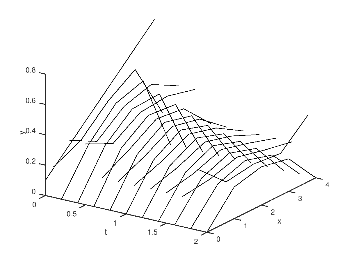
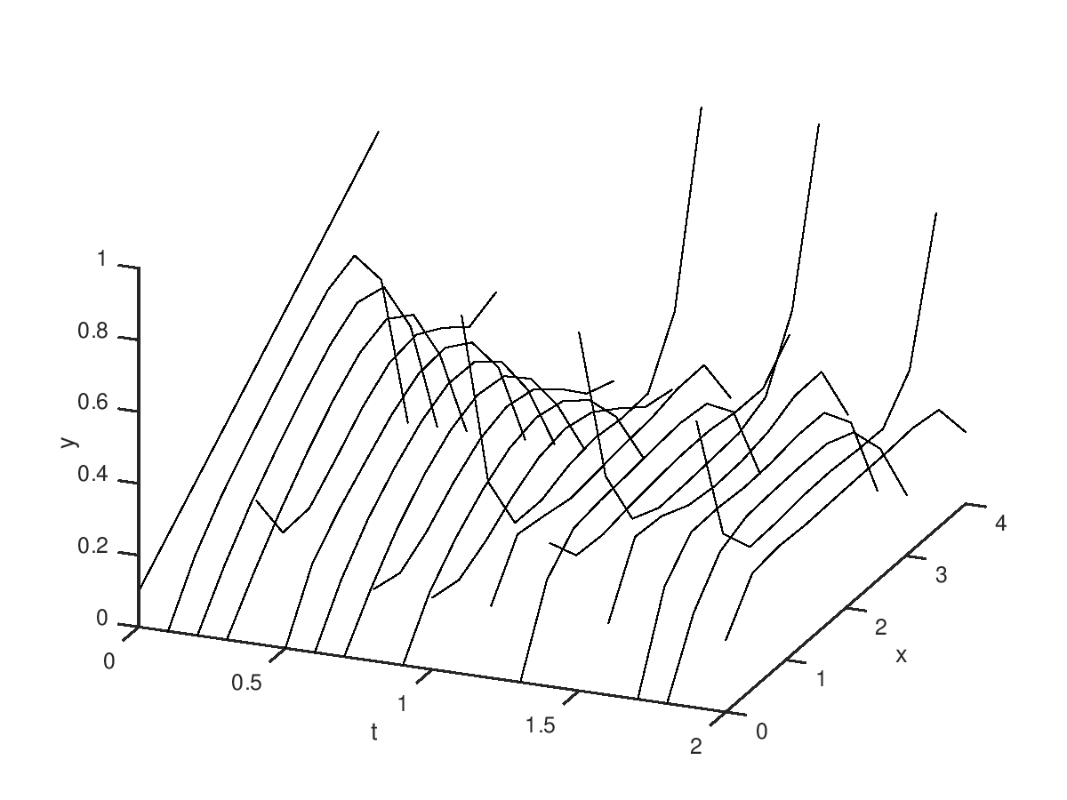
The error bound $E_{\varepsilon}(T)$ is thus linear in $k=T/\tau$. In order to decrease $k$, one can apply consecutively $p\geq 2$ modes in a row (without intermediate $\varepsilon$-approximation); this is equivalent to divide $k$ by $p$, at the price of considering $m^{p}$ “extended” modes instead of just $m$ modes. (see Example 1, Figure 2). An alternative for decreasing $k$ is to increase $\tau$ (which may require in turn to decrease $\Delta t$ for preserving assumption $\Delta t\leq G_{u}(1-\alpha_{u})$, see Remark 4).

Example 1

Consider the 1D reaction-diffusion system with Dirichlet boundary condition (see [45], bistable case):

$$\frac{\partial y(t,x)}{\partial t}=\sigma\frac{\partial^{2}y(t,x)}{\partial x^{2}}+f(y(t,x)),\ \ \ t\in[0,T],\ x\in[0,L]$$

$$y(t,0)=u_{0},\quad y(t,L)=u_{L},$$

$$y(0,x)=y_{0}(x),\ \ \ x\in[0,L]$$

with $\sigma=1,L=4$ and $f(y)=y(1-y)(y-\theta)$ with $\theta=0.3$. The control switching period is $\tau=0.1$. The values of the boundary control $u=(u_{0},u_{L})$ are in

$$U=\{(0,0),(0.2,0.2),(0.4,0.4),(0.6,0.6),(0.8.0.8),(1,1)\}.$$

We discretize the domain $\Omega=[0,L]$ of the system with $M_{1}=5$ discrete points, using a finite difference scheme. Our program returns an OSL constant $\lambda_{u}=-0.322$ for all $u\in U$. Constant $C_{u}$ varies between $10.33$ and $11.85$ depending on the values of $u$.

We then discretize each interval component of the space $S=[0,1]^{M_{1}}$ of values of $y$ into 15 points with spacing $\eta=1/15\approx 0.066$. The grid ${\cal X}$ is of the form $\{0,\eta,2\eta,\dots,15\eta\}^{M_{1}}$, and the initial error $e_{0}$ equal to $\varepsilon=\sqrt{M_{1}}\eta/2$. This leads to $G_{u}$ varying between $0.00155$ and $0.00178$ depending on the value of $u\in U$. One checks: $\frac{|\lambda_{u}|G_{u}}{4}<1$ for all $u\in U$. The time step upper bound required by Theorem 2.1 for ensuring numeric stability is $0.00155$. Since the switching period is $\tau=0.1$, we perform subsampling (see, e.g., [33]) by decomposing every time step $[i\tau,(i+1)\tau)$ ($1\leq i\leq k-1$) into a sequence of elementary Euler steps of length $\Delta t=\tau/100<0.00155$. This ensures that the system satisfies $(H)$, hence, by Theorem 2.1, the explicit Euler scheme is stable and error $\|Y^{\pi}_{t,y_{0}}-\tilde{Y}_{t,z_{0}}^{\pi}\|$ never exceeds $\varepsilon$.

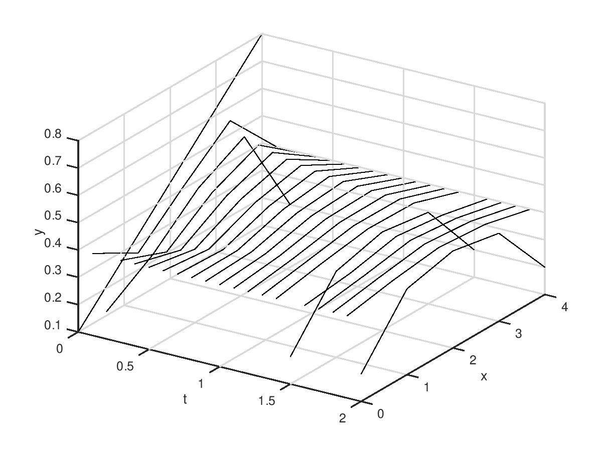
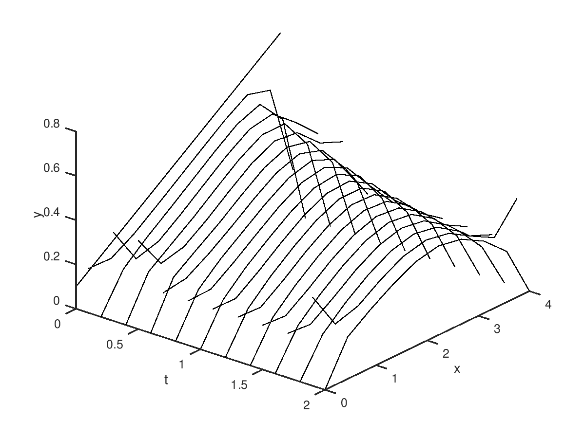
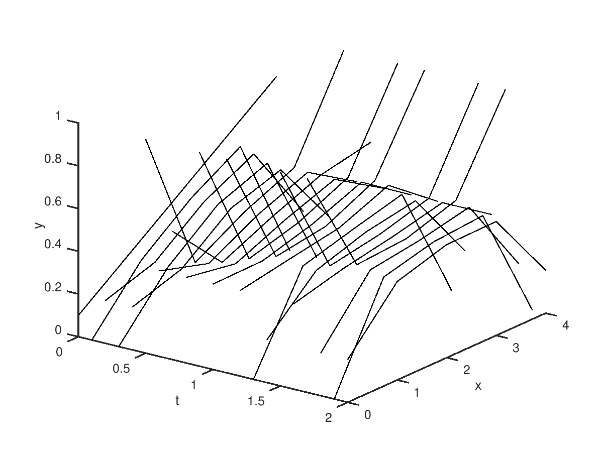
For objective with $y_{f}=(0.3,0.3,0.3,0.3,0.3)$ and horizon time $T=k\tau=2$ (i.e., $k=20$), our program returns an approximate optimal controller in $2$ minutes. Let $z_{0}$ be the $\varepsilon$-representative of $y_{0}=0.8x/L+0.1(1-x/L)$. Let $\pi_{k}^{\varepsilon}$ be the pattern output by $PROC_{k}^{\varepsilon}(z_{0})$. A simulation of $z(t):=\tilde{Y}_{t,z_{0}}^{\pi_{k}^{\varepsilon}}$ is given in Figure 1 with $T=2$, $\tau=0.1$ ($k=20$), $\Delta t=\frac{\tau}{100}$. We have $\|z(T)-yf\|\approx 0.276$. The simulation presents some similarity with simulations displayed in [45] (see, e.g., lower part of Figure 6), with a phase control $u_{0}=u_{L}>\theta$ (here, $u_{0}=u_{L}=0.4$) alternating with a phase control $u_{0}=u_{L}<\theta$ (here, $u_{0}=u_{L}=0.2$). The discretization error $E_{\varepsilon}(T)$ is smaller than $(2k+1)\varepsilon=41\sqrt{5}/30<3.1$.

Figure 1: Simulation of the system of Example 1 discretized with $M_{1}=5$ points, for initial condition $y_{0}=0.8x/L+0.1(1-x/L)$, objective $y_{f}=0.3$ and horizon time $T=2$ ($\tau=0.1$, $\Delta t=\frac{\tau}{100}$).

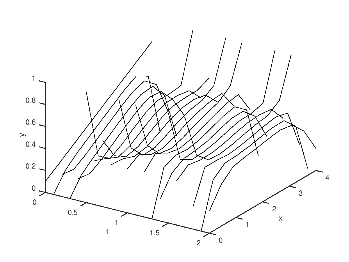
Let us now proceed with extended modes of length $p=2$ and $p=4$, as explained in Remark 5. For $p=2$ (i.e., $k=10$), the control is synthesized in 7mn of CPU time. The controller simulation is given in the left part of Figure 2; we have: $\|z(T)-y_{f}\|\approx 0.445$ with $E_{\varepsilon}(T)<1.57$. For $p=4$ (i.e., $k=5$), the computation of the control requires 8h of CPU time. The corresponding simulation is given in the right part of Figure 2; we now have: $\|z(T)-y_{f}\|\approx 0.164$ with $E_{\varepsilon}(T)<0.82$.

2.5 Model reduction

Let us consider the system ${\cal S}_{2}$ on space $S_{h_{2}}=[0,1]^{M_{2}}$ (with $M_{2}$ even). The differential equation can be written under the form:

$$\frac{dy_{2}}{dt}=\sigma{\cal L}_{h_{2}}y_{2}+\varphi_{h_{2}}(u)+{f}(y_{2}).$$

where ${\cal L}_{h_{2}}$ corresponds to the $(M_{2}\times M_{2})$ Laplacian matrix, and $h_{2}=\frac{L}{M_{2}+1}$.

Let us consider the “reduced” system ${\cal S}_{1}$ defined on $S_{h_{1}}=[0,1]^{M_{1}}$ with $M_{1}=M_{2}/2$, defined by:

$$\frac{dy_{1}}{dt}=\sigma{\cal L}_{h_{1}}y_{1}+\varphi_{h_{1}}(u)+f({y}_{1}),$$

where ${\cal L}_{h_{1}}$ is the $(M_{1}\times M_{1})$ Laplacian matrix and $h_{1}=\frac{L}{M_{1}+1}$.

With $M_{1}=M_{2}/2$, we have $h_{2}=\frac{L}{2M_{1}+1}$ ($=\frac{h_{1}(M_{1}+1)}{2M_{1}+1}$). Let us consider the $(M_{1}\times M_{2})$ reduction matrix:

$$\Pi:=\frac{1}{\sqrt{2}}\begin{bmatrix}1&1&0&\cdots&0&0\\ 0&0&1&1&\cdots&0\\ \ &\ &\cdots&\ &\ &\ \\ 0&0&\cdots&0&1&1\end{bmatrix}$$

Note that $\Pi\Pi^{\top}={\cal I}_{M}$. Let us consider a point $w_{0}\in S_{h_{2}}$, and let $z_{0}=\Pi w_{0}\in S_{h_{1}}$.

Theorem 2.3

Consider the system ${\cal S}_{2}$ and a point $w_{0}\in S_{h_{2}}$, and let $z_{0}=\Pi w_{0}\in S_{h_{1}}$. Let $Y_{w_{0}}^{h_{2}}$ and $Y_{z_{0}}^{h_{1}}$ be the solutions of ${\cal S}_{2}$ and ${\cal S}_{1}$ with initial conditions $w_{0}\in S_{h_{2}}$ and $z_{0}\in S_{h_{1}}$ respectively. We have:

$$\forall t\geq 0\ \ \ \|\Pi Y_{w_{0}}^{h_{2}}(t)-Y_{z_{0}}^{h_{1}}(t)\|\leq\frac{K_{2}\sigma}{|\lambda_{h_{1}}|},$$

where

$$K_{2}:=\sup_{w\in S_{h_{2}}}\|(\Pi{\cal L}_{h_{2}}-{\cal L}_{h_{1}}\Pi)w\|,$$

and ${\cal L}_{h_{2}}$ (resp. ${\cal L}_{h_{1}}$) is the Laplacian matrix of size $M_{2}\times M_{2}$ (resp. $M_{1}\times M_{1}$).

Proof

Let us consider the system ${\cal S}_{2}$:

$$\frac{dy_{2}}{dt}=\sigma{\cal L}_{h_{2}}y_{2}+\varphi_{h_{2}}(u)+f(y_{2}).$$

By application of the projection matrix $\Pi$, we get:

$$\frac{d\Pi y_{2}}{dt}=\sigma\Pi{\cal L}_{h_{2}}y_{2}+\varphi_{{h_{1}}}(u)+f(\Pi y_{2}).$$

By substracting pairwise with the sides of ${\cal S}_{1}$, we have:

$$\frac{d\Pi y_{2}}{dt}-\frac{dy_{1}}{dt}=\sigma(\Pi{\cal L}_{h_{2}}y_{2}-{\cal L}_{{h_{1}}}y_{1})+f(\Pi y_{2})-f(y_{1})$$

$$=F_{h_{1}}(\Pi y_{2})-F_{h_{1}}(y_{1})+\sigma(\Pi{\cal L}_{h_{2}}-{\cal L}_{h_{1}}\Pi)y_{2},$$

where $F_{h_{1}}(y)=\sigma{\cal L}_{h_{1}}(y)+f(y)$ for $y\in S_{h_{1}}$. On the other hand, we have:

$\frac{1}{2}\frac{d}{dt}(\|\Pi y_{2}-y_{1}\|^{2})=\langle\frac{d}{dt}(\Pi y_{2}-y_{1}),\Pi y_{2}-y_{1}\rangle$

$=\langle F_{h_{1}}(\Pi y_{2})-F_{h_{1}}(y_{1})+\sigma(\Pi{\cal L}_{h_{2}}-{\cal L}_{h_{1}}\Pi)y_{2},\Pi y_{2}-y_{1}\rangle$

$=\langle F_{h_{1}}(\Pi y_{2})-F_{h_{1}}(y_{1}),\Pi y_{2}-y_{1}\rangle$

$+\sigma\langle(\Pi{\cal L}_{h_{2}}-{\cal L}_{h_{1}}\Pi)y_{2},\Pi y_{2}-y_{1}\rangle$

$\leq\lambda_{h_{1}}\|\Pi y_{2}-y_{1}\|^{2}+\sigma\langle(\Pi{\cal L}_{h_{2}}-{\cal L}_{h_{1}}\Pi)y_{2},\Pi y_{2}-y_{1}\rangle$

$\leq\lambda_{h_{1}}\|\Pi y_{2}-y_{1}\|^{2}+K_{2}\sigma\|\Pi y_{2}-y_{1}\|$

$$\mbox{with}\ \ \ \ K_{2}:=\sup_{w\in S_{h_{2}}}\|(\Pi{\cal L}_{h_{2}}-{\cal L}_{{h_{1}}}\Pi)w\|$$

$\leq\lambda_{h_{1}}\|\Pi y_{2}-y_{1}\|^{2}+K_{2}\sigma\frac{1}{2}(\alpha\|\Pi y_{2}-y_{1}\|^{2}+\frac{1}{\alpha})$,
for all $\alpha>0$. Choosing $\alpha>0$ such that $K_{2}\sigma\alpha=-\lambda_{h_{1}}$, i.e.: $\alpha=-\frac{\lambda_{h_{1}}}{K_{2}\sigma}$, we have:

$$\frac{1}{2}\frac{d}{dt}(\|\Pi y_{2}-y_{1}\|^{2})\leq\frac{\lambda_{h_{1}}}{2}\|\Pi y_{2}-y_{1}\|^{2}-\frac{(K_{2}\sigma)^{2}}{2\lambda_{h_{1}}}.$$

Since $y_{2}(0)=w_{0}$ and $y_{1}(0)=z_{0}$, we get by integration:

$$\|\Pi y_{2}(t)-y_{1}(t)\|^{2}\leq\frac{(K_{2}\sigma)^{2}}{\lambda_{h_{1}}^{2}}(1-e^{\lambda_{h_{1}}t})\leq\frac{(K_{2}\sigma)^{2}}{\lambda_{h_{1}}^{2}}.$$

Hence: $\|\Pi Y^{h_{2}}_{w_{0}}(t)-Y_{z_{0}}^{h_{1}}(t)\|\leq\frac{K_{2}\sigma}{|\lambda_{{h_{1}}}|}$ for all $t\geq 0$. $\Box$

This proposition expresses that the reduction error is bounded by constant $\frac{K_{2}\sigma}{|\lambda_{{h_{1}}}|}$ when the same control modes are applied to both systems.

Let $y_{2}^{0}\in S_{2}$ and $y_{2}^{f}\in S_{2}$ be an initial and objective point respectively. Let $y_{1}^{0}:=\Pi y_{2}^{0}\in S_{1}$ and $y_{1}^{f}:=\Pi y_{2}^{f}\in S_{1}$ denote their projections. Suppose that $\pi^{\varepsilon}$ is the pattern returned by $PROC^{\varepsilon}_{k}(y_{1}^{0})$ for the reduced system ${\cal S}_{1}$. Then, from Theorem 2.3, it follows that, when the same control $\pi^{\varepsilon}$ is applied to the original system ${\cal S}_{2}$ with $y_{2}(0)=y_{2}^{0}\in S_{2}$, it makes the projection $\Pi y_{2}^{\pi^{\varepsilon}}(t)\in S_{1}$ reach a neighborhood of $y_{1}^{f}$ at time $t=T$. Formally, we have:

$$\|Py_{2}^{\pi^{\varepsilon}}(T)-y_{1}^{f}\|\leq\|y_{1}^{\pi^{\varepsilon}}(T)-y_{1}^{f}\|+\frac{K_{2}\sigma}{|\lambda_{{h_{1}}}|}.$$

Example 2

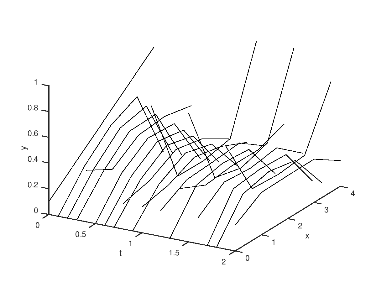
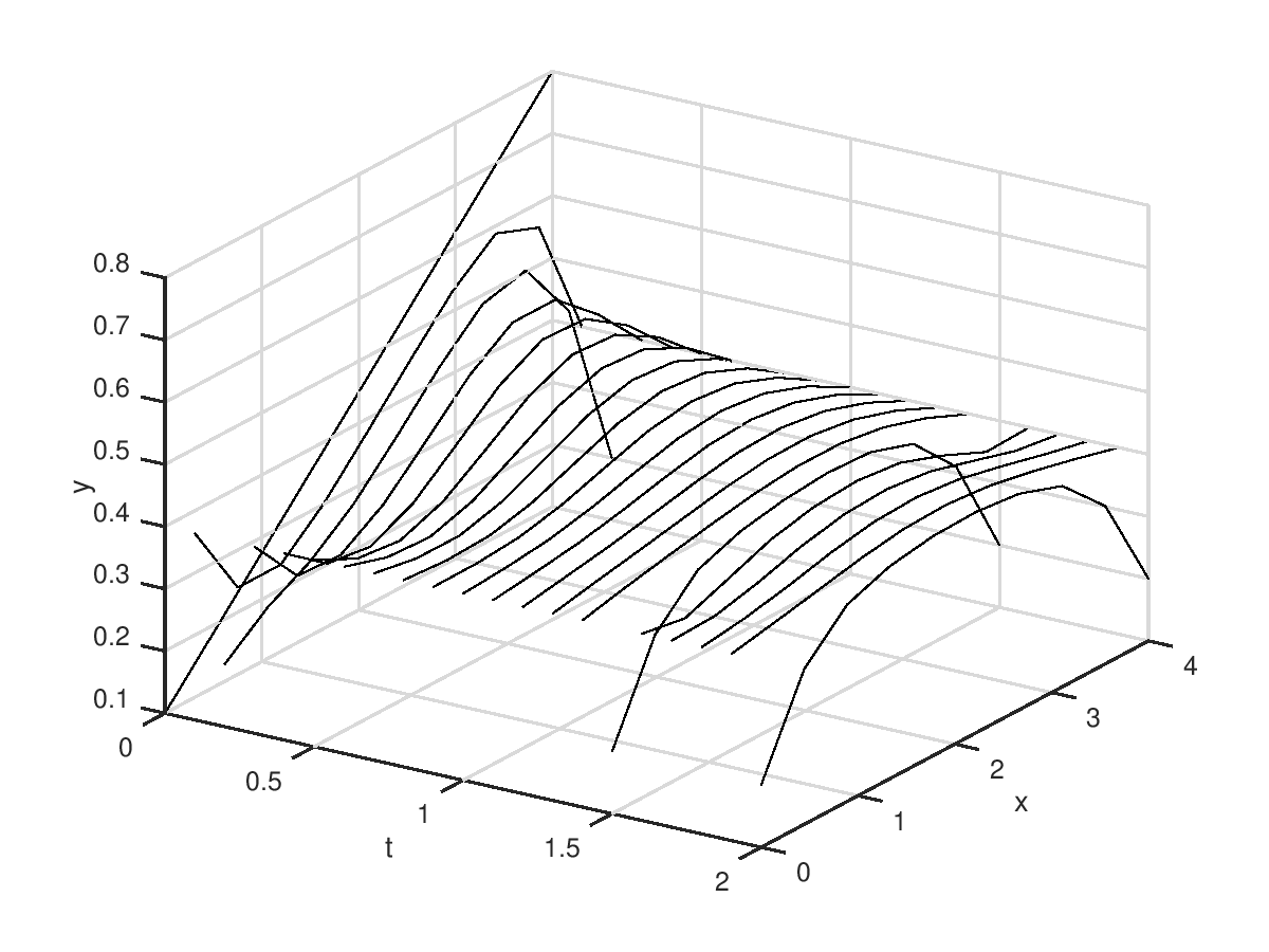
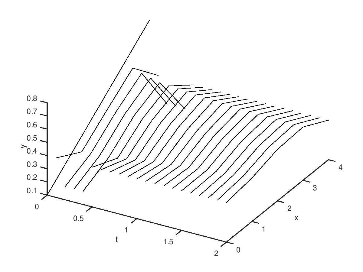
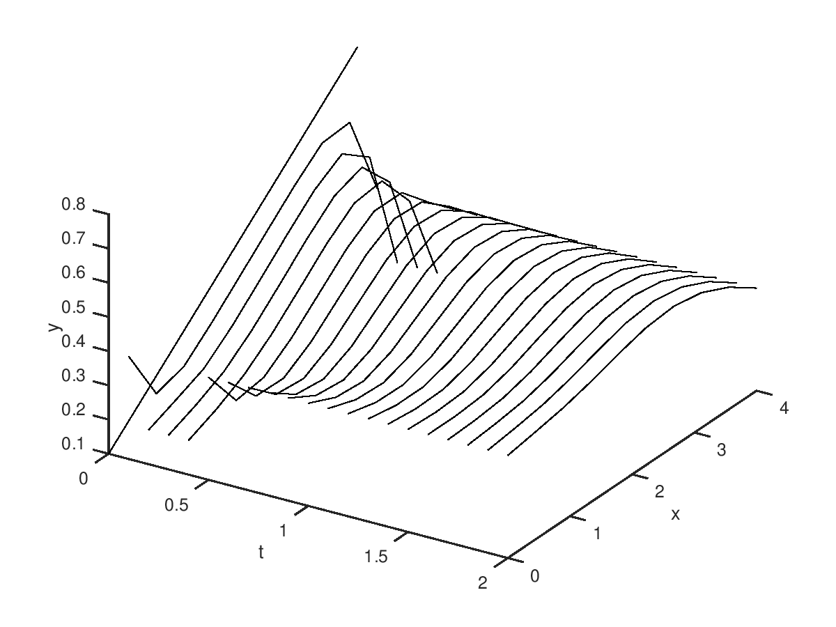
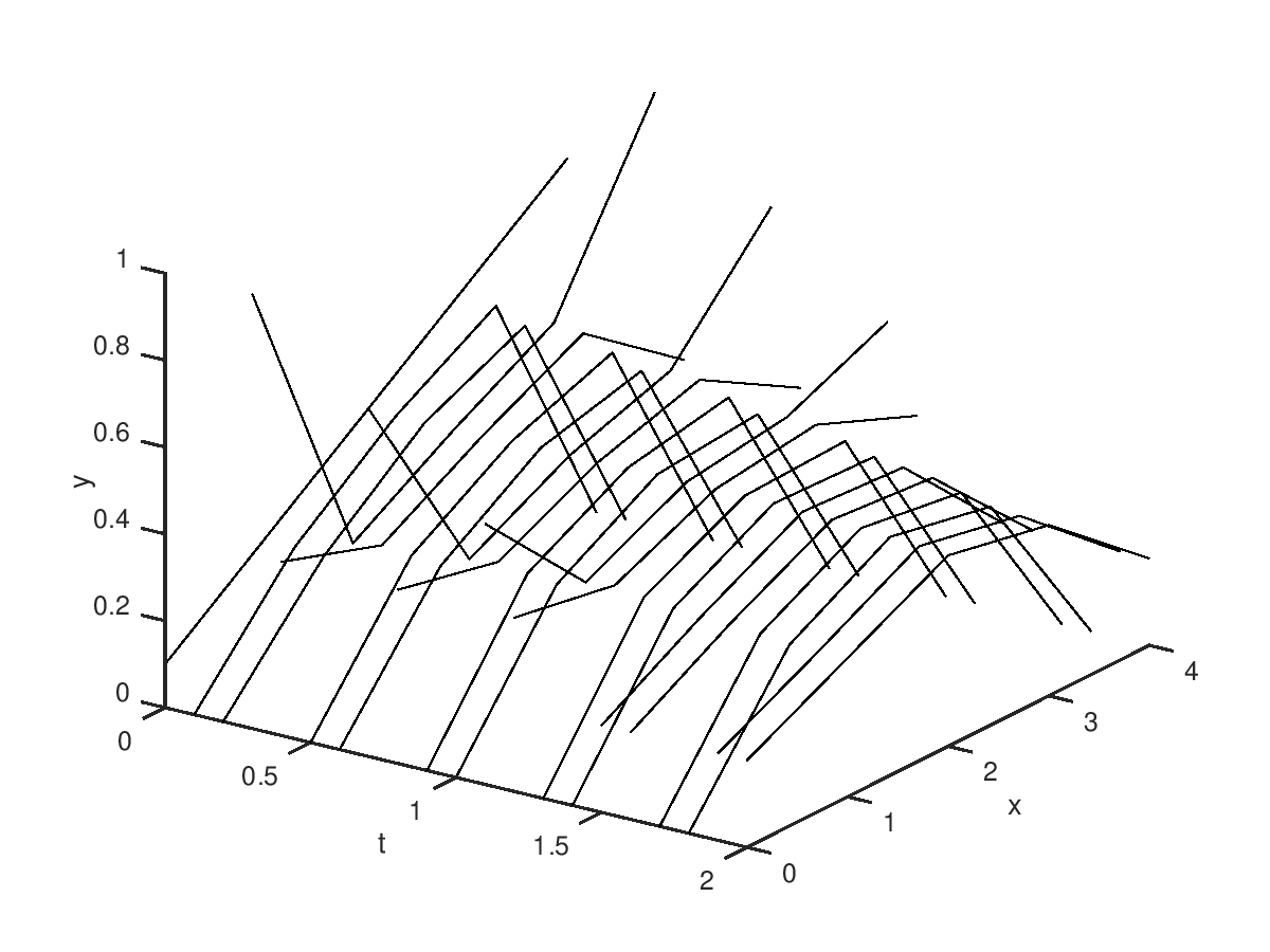
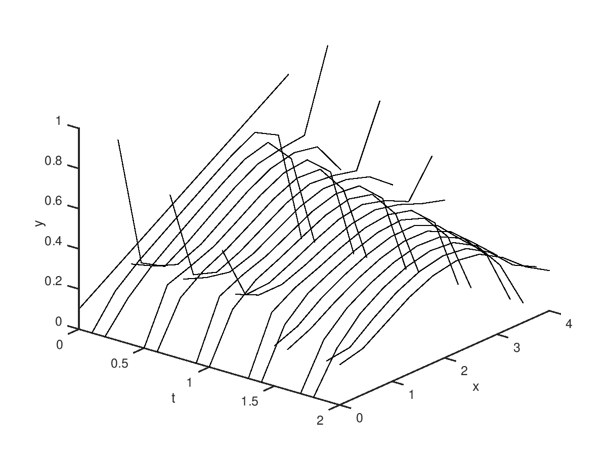
Let us take the system defined in Example 1 as reduced system ${\cal S}_{1}$ ($M_{1}=5$), and let us take as “full-size” system ${\cal S}_{2}$ the system corresponding to $M_{2}=10$. Since the size of the grid ${\cal X}_{2}$ associated to ${\cal S}_{2}$ is exponential in $M_{2}$, the size ${\cal X}_{2}$ is multiplied by $(1/\eta)^{M_{2}-M_{1}}=15^{5}\approx 7.6\cdot 10^{5}$ w.r.t. the size of the grid ${\cal X}_{1}$ associated to ${\cal S}_{1}$. The complexity for synthesizing directly the optimal control of ${\cal S}_{2}$ thus becomes intractable. On the other hand, if we apply to ${\cal S}_{2}$ the optimal strategy $\pi^{\varepsilon}\in U^{k}$ found for ${\cal S}_{1}$ in Example 1, we obtain a simulation depicted in Figure 3 for extended mode of length 1, which is the counterpart of Figure 1 with $M_{2}=10$ (instead of $M_{1}=5$), and has a very similar form. Likewise, if we apply to ${\cal S}_{2}$ the optimal strategy $\pi^{\varepsilon}\in U^{k}$ found for ${\cal S}_{1}$ in Example 1, we obtain a simulation depicted in Figure 4 for extended modes of length 2 and 4, which is the counterpart of Figure 2, and very similar to it. As seen above, we have:

$$\|\Pi y_{2}^{\pi^{\varepsilon}}(T)-y_{1}^{f}\|\leq\|y_{1}^{\pi^{\varepsilon}}(T)-y_{1}^{f}\|+\frac{K_{2}\sigma}{|\lambda_{{h_{1}}}|},$$

where $y_{1}^{f}=(0.3,0.3,0.3,0.3,0.3)$, and the reduction error is bounded by $\frac{K_{2}\sigma}{|\lambda_{{h_{1}}}|}=17.9\ \sigma.$

The subexpression $\|y_{1}^{\pi^{\varepsilon}}(T)-y_{1}^{f}\|$ can be computed a posteriori by simulation: see Table 1 of Appendix 2, with $\sigma=1$, $\sigma=0.5$. The value of $\|y_{2}^{\pi^{\varepsilon}}(T)-y_{2}^{f}\|$ for ${\cal S}_{2}$ is also given in Table 1 for comparison.

The upper bound $\|y_{1}^{\pi^{\varepsilon}}(T)-y_{1}^{f}\|+\frac{K_{2}\sigma}{|\lambda_{{h_{1}}}|}$ of the distance $\|Py_{2}^{\pi^{\varepsilon}}(T)-y_{1}^{f}\|$ is very conservative, due to a priori error bound $\frac{K_{2}\sigma}{|\lambda_{{h_{1}}}|}$. On can obtain a posteriori a much sharper estimate of $\|Py^{\pi^{\varepsilon}}_{2}(T)-y_{1}^{f}\|$ by simulation: see Table 2, Appendix 2.

Figure 2: Simulation of the system of Example 1 discretized with $M_{1}=5$ points, with extended modes of length 2 (left) and extended modes of length 4 (right).

Figure 3: Simulation of the system of Ex. 1, discretized with $M_{2}=10$ points, with extended mode of length 1.

Figure 4: Simulation of the system of Ex. 1, discretized with $M_{2}=10$ points, with extended modes of length 2 (left) and extended modes of length 4 (right).

3 Final Remarks

Using the notion of OSL constant, we have shown how to use the finite difference and explicit Euler methods in order to solve finite horizon control problems for reaction-diffusion equations. Furthermore, we have quantified the deviation of this control with the optimal strategy, and proved that the error upper bound is linear in the horizon length. We have applied the method to a 1D bi-stable reaction-diffusion equation, and have found experimental results similar to those of [45]. We have also given a simple and specific model reduction method which allows to apply the method to equations of larger size. In future work, we plan to apply the method to 2D reaction-diffusion equations (e.g., Test 1 of [2]).

Appendix 1: Proof of Lemma 1

Proof

It is easy to check that $0<\alpha_{u}<1$ when $\frac{|\lambda_{u}|G_{u}}{4}<1$.

Let $t^{*}:=G_{u}(1-\alpha_{u})$. Let us first prove $\delta_{e_{0}}(t)\leq e_{0}$ for $t=t^{*}$. We have:

$$-\frac{1}{2}|\lambda_{u}|G_{u}+(2+\frac{1}{2}|\lambda_{u}|G_{u})\alpha_{u}-\alpha_{u}^{2}=0.$$

Hence:

$$\frac{1}{2G_{u}(1-\alpha_{u})}\lambda_{u}G_{u}^{2}(1-\alpha_{u})^{2}+2\alpha_{u}-\alpha_{u}^{2}=0,$$

i.e.

$$\frac{1}{2t^{*}}\lambda_{u}(t^{*})^{2}+2\alpha_{u}-\alpha_{u}^{2}=0.$$

We have: $-\frac{1}{4G_{u}^{2}t^{*}}\lambda_{u}(t^{*})^{4}e^{\lambda_{u}t^{*}}\geq 0$. It follows:

$$\frac{1}{2t^{*}}\lambda_{u}(t^{*})^{2}+2\alpha_{u}-\alpha_{u}^{2}-\frac{1}{4G_{u}^{2}t^{*}}\lambda_{u}(t^{*})^{4}e^{\lambda_{u}t^{*}}\geq 0.$$

Hence:

$$1+\frac{1}{2t^{*}}\lambda_{u}(t^{*})^{2}-\frac{1}{G_{u}^{2}}((t^{*})^{2}+\frac{1}{4t^{*}}\lambda_{u}(t^{*})^{4}e^{\lambda_{u}t^{*}})\geq 0.$$

By multiplying by $t^{*}$:

$$(t^{*}+\frac{1}{2}\lambda_{u}(t^{*})^{2})-\frac{1}{G_{u}^{2}}((t^{*})^{3}+\frac{1}{4}\lambda_{u}(t^{*})^{4}e^{\lambda_{u}t^{*}})\geq 0.$$

Since $G=\sqrt{3}|\lambda_{u}|e_{0}/C_{u}$:

$$e_{0}^{2}(t^{*}+\frac{1}{2}\lambda_{u}(t^{*})^{2})+\frac{C_{u}^{2}}{\lambda_{u}^{2}}(-\frac{1}{3}(t^{*})^{3}-\frac{1}{12}\lambda_{u}(t^{*})^{4}e^{\lambda_{u}t^{*}})\geq 0.$$

By multiplying by $\lambda_{u}$:

$$e_{0}^{2}(\lambda_{u}t^{*}+\frac{1}{2}\lambda_{u}^{2}(t^{*})^{2})+\frac{C_{u}^{2}}{\lambda_{u}^{2}}(-\frac{1}{3}\lambda_{u}(t^{*})^{3}-\frac{1}{12}\lambda_{u}^{2}(t^{*})^{4}e^{\lambda_{u}t^{*}})\leq 0.$$

Note that, in the above formula, the subexpression $\lambda_{u}t^{*}+\frac{1}{2}\lambda_{u}^{2}(t^{*})^{2}$ is such that:

$$\lambda_{u}t^{*}+\frac{1}{2}\lambda_{u}^{2}(t^{*})^{2}\geq e^{\lambda_{u}t^{*}}-1$$

since $e^{\lambda_{u}t^{*}}-1=\lambda_{u}t^{*}+\frac{1}{2}\lambda_{u}^{2}(t^{*})^{2}e^{\lambda\theta}\leq\lambda_{u}t^{*}+\frac{1}{2}\lambda_{u}^{2}(t^{*})^{2}$.

On the other hand, the subexpression $-\frac{1}{3}\lambda_{u}(t^{*})^{3}-\frac{1}{12}\lambda_{u}^{2}(t^{*})^{4}e^{\lambda_{u}t^{*}}$ is such that:

$$-\frac{1}{3}\lambda_{u}(t^{*})^{3}-\frac{1}{12}\lambda_{u}^{2}(t^{*})^{4}e^{\lambda_{u}t^{*}}\geq\frac{2t^{*}}{\lambda_{u}}+(t^{*})^{2}+\frac{2}{\lambda_{u}^{2}}(1-e^{\lambda_{u}t^{*}})$$

since

$\frac{2t^{*}}{\lambda_{u}}+(t^{*})^{2}+\frac{2}{\lambda_{u}^{2}}(1-e^{\lambda_{u}t^{*}})$

$=\frac{2t^{*}}{\lambda_{u}}+(t^{*})^{2}+\frac{2}{\lambda_{u}^{2}}(-\lambda_{u}t^{*}-\frac{1}{2}\lambda_{u}^{2}(t^{*})^{2}-\frac{1}{6}\lambda_{u}^{3}(t^{*})^{3}-\frac{1}{24}\lambda_{u}^{4}(t^{*})^{4}e^{\lambda_{u}\theta}$

$=\frac{2}{\lambda_{u}^{2}}(-\frac{1}{6}\lambda_{u}^{3}(t^{*})^{3}-\frac{1}{24}\lambda_{u}^{4}(t^{*})^{4}e^{\lambda_{u}\theta})$ for some $0\leq\theta\leq t^{*}$

$=-\frac{1}{3}\lambda_{u}(t^{*})^{3}-\frac{1}{12}\lambda_{u}^{2}(t^{*})^{4}e^{\lambda_{u}\theta}$

$\leq-\frac{1}{3}\lambda_{u}(t^{*})^{3}-\frac{1}{12}\lambda_{u}^{2}(t^{*})^{4}e^{\lambda_{u}t^{*}}.$

It follows:

$$e_{0}^{2}(e^{\lambda_{u}t^{*}}-1)+\frac{C_{u}^{2}}{\lambda_{u}^{2}}(\frac{2t^{*}}{\lambda_{u}}+(t^{*})^{2}+\frac{2}{\lambda_{u}^{2}}(1-e^{\lambda_{u}t^{*}}))\leq 0.$$

$$e_{0}^{2}e^{\lambda_{u}t^{*}}+\frac{C_{u}^{2}}{\lambda_{u}^{2}}(\frac{2t^{*}}{\lambda_{u}}+(t^{*})^{2}+\frac{2}{\lambda_{u}^{2}}(1-e^{\lambda_{u}t^{*}}))\leq e_{0}^{2}.$$

i.e.

$$(\delta_{e_{0}}^{u}(t^{*}))^{2}\leq e_{0}^{2}.$$

Hence: $\delta_{e_{0}}^{u}(t^{*})\leq e_{0}.$ It remains to show: $\delta_{e_{0}}^{u}(t)\leq e_{0}$ for $t\in[0,t^{*}]$.

Consider the 1rst and 2nd derivative $\delta^{\prime}(\cdot)$ and $\delta^{\prime\prime}(\cdot)$ of $\delta(\cdot)$. We have:

$\delta^{\prime}(t)=\lambda_{u}e_{0}^{2}e^{\lambda_{u}t}+\frac{C_{u}^{2}}{\lambda_{u}^{2}}(2t+\frac{2}{\lambda_{u}}-\frac{2}{\lambda_{u}}e^{\lambda_{u}t})$

$\delta^{\prime\prime}(t)=\lambda_{u}^{2}e_{0}^{2}e^{\lambda_{u}t}+\frac{C_{u}^{2}}{\lambda_{u}^{2}}(2-2e^{\lambda_{u}t}).$

Hence $\delta^{\prime\prime}(t)>0$ for all $t\geq 0$. On the other hand, for $t=0$, $\delta^{\prime}(t)=\lambda_{u}e_{0}^{2}<0$, and for $t$ sufficiently large, $\delta^{\prime}(t)>0$. Hence, $\delta^{\prime}(\cdot)$ is strictly increasing and has a unique root. It follows that the equation $\delta(t)=e_{0}$ has a unique solution $t^{**}$ for $t>0$. Besides, $\delta(t)\leq e_{0}$ for $t\in[0,t^{**}]$, and $\delta(t)\geq e_{0}$ for $t\in[t^{**},+\infty)$. Since we have shown: $\delta(t^{*})\leq e_{0}$, it follows $t^{*}\leq t^{**}$ and $\delta(t)\leq e_{0}$ for $t\in[0,t^{*}]$.

$\Box$

Appendix 2: Numerical results

Dimension	Extended mode length	$\|y_{i}^{\pi^{\varepsilon}}(T)-y_{i}^{f}\|$ for $\sigma=1$	$\|y_{i}^{\pi^{\varepsilon}}(T)-y_{i}^{f}\|$ for $\sigma=0.5$
$i=1\ (M_{i}=5)$	1	0.27642	0.33869
	2	0.44496	0.39068
	4	0.15294	0.22024
$i=2\ (M_{i}=10)$	1	0.39904	0.50251
	2	0.50092	0.58500
	4	0.16738	0.31440

Table 1: Value $\|y_{i}^{\pi^{\varepsilon}}(T)-y_{i}^{f}\|$ for $\sigma=1$ and $\sigma=0.5$ ($T=2$, $i=1,2$).

Extended mode length	$\|P{y}^{\pi^{\varepsilon}}_{2}(T)-y_{1}^{f}\|$ for $\sigma=1$	$\|P{y}^{\pi^{\varepsilon}}_{2}(T)-y_{1}^{f}\|$ for $\sigma=0.5$
1	0.67429	0.77322
2	0.27501	0.72322
4	0.31385	0.21481

Table 2: Projection value $\|P{y}^{\pi^{\varepsilon}}_{2}(T)-y_{1}^{f}\|$ for $\sigma=1$, $\sigma=0.5$ ($T=2$).

Length 1, $M_{1}=5$	Length 1, $M_{2}=10$
Length 2, $M_{1}=5$	Length 2, $M_{2}=10$
Length 4, $M_{1}=5$	Length 4, $M_{2}=10$

Figure 5: Simulation of the controllers for $\sigma=1$.

Length 1, $M_{1}=5$	Length 1, $M_{2}=10$
Length 2, $M_{1}=5$	Length 2, $M_{2}=10$
Length 4, $M_{1}=5$	Length 4, $M_{2}=10$

Figure 6: Simulation of the controllers for $\sigma=0.5$.

References

- [1] Alessandro Alla, Maurizio Falcone, and Stefan Volkwein. Error analysis for POD approximations of infinite horizon problems via the dynamic programming approach. SIAM J. Control and Optimization, 55(5):3091–3115, 2017.
- [2] Alessandro Alla and Luca Saluzzi. A HJB-POD approach for the control of nonlinear PDEs on a tree structure. CoRR, abs/1905.03395, 2019.
- [3] Matthias Althoff. Reachability analysis of large linear systems with uncertain inputs in the Krylov subspace. CoRR, abs/1712.00369, 2017.
- [4] Matthias Althoff, Olaf Stursberg, and Martin Buss. Reachability analysis of nonlinear systems with uncertain parameters using conservative linearization. In Proceedings of the 47th IEEE Conference on Decision and Control, CDC 2008, December 9-11, 2008, Cancún, Mexico, pages 4042–4048. IEEE, 2008.
- [5] Zahra Aminzare, Yusef Shafi, Murat Arcak, and Eduardo D Sontag. Guaranteeing spatial uniformity in reaction-diffusion systems using weighted norm contractions. In A Systems Theoretic Approach to Systems and Synthetic Biology I: Models and System Characterizations, pages 73–101. Springer, 2014.
- [6] Zahra Aminzare and Eduardo D Sontag. Logarithmic lipschitz norms and diffusion-induced instability. Nonlinear Analysis: Theory, Methods & Applications, 83:31–49, 2013.
- [7] Zahra Aminzare and Eduardo D Sontag. Some remarks on spatial uniformity of solutions of reaction–diffusion pdes. Nonlinear Analysis: Theory, Methods & Applications, 147:125–144, 2016.
- [8] Murat Arcak. Certifying spatially uniform behavior in reaction–diffusion pde and compartmental ode systems. Automatica, 47(6):1219–1229, 2011.
- [9] Werner Barthel, Christian John, and Fredi Tröltzsch. Optimal boundary control of a system of reaction diffusion equations. ZAMM - Journal of Applied Mathematics and Mechanics / Zeitschrift für Angewandte Mathematik und Mechanik, 90(12):966–982, 2010.
- [10] Richard Bellman. Dynamic Programming. Princeton University Press, Princeton, NJ, USA, 1 edition, 1957.
- [11] Martin Berz and Georg Hoffstätter. Computation and application of taylor polynomials with interval remainder bounds. Reliable Computing, 4(1):83–97, 1998.
- [12] Martin Berz and Kyoko Makino. Verified integration of ODEs and flows using differential algebraic methods on high-order Taylor models. Reliable Computing, 4(4):361–369, 1998.
- [13] Eduardo Casas, Christopher Ryll, and Fredi Tröltzsch. Optimal control of a class of reaction-diffusion systems. Comp. Opt. and Appl., 70(3):677–707, 2018.
- [14] Adrien Le Coënt and Laurent Fribourg. Guaranteed control of sampled switched systems using semi-Lagrangian schemes and one-sided Lipschitz constants. In 58th IEEE Conference on Decision and Control, CDC 2019, Nice, France, December 11-13, 2019.
- [15] Sébastien Court, Karl Kunisch, and Laurent Pfeiffer. Hybrid optimal control problems for a class of semilinear parabolic equations. Discrete & Continuous Dynamical Systems - S, 11, 2018.
- [16] Jorge Estrela da Silva, Joao Tasso Sousa, and Fernando Lobo Pereira. Synthesis of safe controllers for nonlinear systems using dynamic programming techniques. In 8th International Conference on Physics and Control (PhysCon 2017). IPACS Electronic library, 2017.
- [17] Germund Dahlquist. Stability and error bounds in the numerical integration of ordinary differential equations. PhD thesis, Almqvist & Wiksell, 1958.
- [18] Maurizio Falcone and Tiziana Giorgi. An approximation scheme for evolutive hamilton-jacobi equations. In Stochastic analysis, control, optimization and applications, pages 289–303. Springer, 1999.
- [19] Chuchu Fan, James Kapinski, Xiaoqing Jin, and Sayan Mitra. Simulation-driven reachability using matrix measures. ACM Transactions on Embedded Computing Systems (TECS), 17(1):21, 2018.
- [20] Heather Finotti, Suzanne Lenhart, and Tuoc Van Phan. Optimal control of advective direction in reaction-diffusion population models. Evolution Equations & Control Theory, 1, 2012.
- [21] Antoine Girard. Reachability of uncertain linear systems using zonotopes. In Proc. of Hybrid Systems: Computation and Control, volume 3414 of LNCS, pages 291–305. Springer, 2005.
- [22] Roland Griesse and Stefan Volkwein. A primal-dual active set strategy for optimal boundary control of a nonlinear reaction-diffusion system. SIAM J. Control and Optimization, 44(2):467–494, 2005.
- [23] Zhi Han and Bruce H. Krogh. Reachability analysis of hybrid control systems using reduced-order models. In Proceedings of the 2004 American Control Conference, volume 2, pages 1183–1189 vol.2, June 2004.
- [24] Zhi Han and Bruce H. Krogh. Reachability analysis of large-scale affine systems using low-dimensional polytopes. In Hybrid Systems: Computation and Control, 9th International Workshop, HSCC 2006, Santa Barbara, CA, USA, March 29-31, 2006, Proceedings, pages 287–301, 2006.
- [25] Dante Kalise and Axel Kröner. Reduced-order minimum time control of advection-reaction-diffusion systems via dynamic programming. In 21st International Symposium on Mathematical Theory of Networks and Systems, pages 1196–1202, Groningen, Netherlands, July 2014.
- [26] Dante Kalise and Karl Kunisch. Polynomial approximation of high-dimensional hamilton-jacobi-bellman equations and applications to feedback control of semilinear parabolic pdes. SIAM J. Scientific Computing, 40(2), 2018.
- [27] Tomasz Kapela and Piotr Zgliczyński. A lohner-type algorithm for control systems and ordinary differential inclusions. Discrete & Continuous Dynamical Systems-B, 11(2):365–385, 2009.
- [28] Toshiyuki Koto. IMEX Runge-Kutta schemes for reaction-diffusion equations. Journal of Computational and Applied Mathematics, 215(1):182–195, 2008.
- [29] W. Kühn. Rigorously computed orbits of dynamical systems without the wrapping effect. Computing, 61(1):47–67, 1998.
- [30] Karl Kunisch, Stefan Volkwein, and Lei Xie. Hjb-pod-based feedback design for the optimal control of evolution problems. SIAM J. Applied Dynamical Systems, 3(4):701–722, 2004.
- [31] Adrien Le Coënt. OSLator 1.0. https://bitbucket.org/alecoent/oslator/src/master/, 2019.
- [32] Adrien Le Coënt, Julien Alexandre Dit Sandretto, Alexandre Chapoutot, Laurent Fribourg, Florian De Vuyst, and Ludovic Chamoin. Distributed control synthesis using Euler’s method. In Proc. of International Workshop on Reachability Problems (RP’17), volume 247 of Lecture Notes in Computer Science, pages 118–131. Springer, 2017.
- [33] Adrien Le Coënt, Florian De Vuyst, Ludovic Chamoin, and Laurent Fribourg. Control synthesis of nonlinear sampled switched systems using Euler’s method. In Proc. of International Workshop on Symbolic and Numerical Methods for Reachability Analysis (SNR’17), volume 247 of EPTCS, pages 18–33. Open Publishing Association, 2017.
- [34] Adrien Le Coënt, Florian De Vuyst, Christian Rey, Ludovic Chamoin, and Laurent Fribourg. Guaranteed control synthesis of switched control systems using model order reduction and state-space bisection. In Proc. of International Workshop on Synthesis of Complex Parameters (SYNCOP’15), volume 44 of OASICS, pages 33–47. Schloss Dagstuhl – Leibniz-Zentrum für Informatik, 2015.
- [35] Rudolf J. Lohner. Enclosing the solutions of ordinary initial and boundary value problems. Computer Arithmetic, pages 255–286, 1987.
- [36] Sergei Mikhailovich Lozinskii. Error estimate for numerical integration of ordinary differential equations. i. Izvestiya Vysshikh Uchebnykh Zavedenii. Matematika, (5):52–90, 1958.
- [37] John Maidens and Murat Arcak. Reachability analysis of nonlinear systems using matrix measures. IEEE Transactions on Automatic Control, 60(1):265–270, 2014.
- [38] Ian M. Mitchell, Alexandre M. Bayen, and Claire J. Tomlin. Validating a hamilton-jacobi approximation to hybrid system reachable sets. In Hybrid Systems: Computation and Control, 4th International Workshop, HSCC 2001, Rome, Italy, March 28-30, 2001, Proceedings, pages 418–432, 2001.
- [39] Ian M. Mitchell and Claire Tomlin. Overapproximating reachable sets by hamilton-jacobi projections. J. Sci. Comput., 19(1-3):323–346, 2003.
- [40] Ramon Moore. Interval Analysis. Prentice Hall, 1966.
- [41] Scott J. Moura and Hosam K. Fathy. Optimal boundary control & estimation of diffusion-reaction pdes. In Proceedings of the 2011 American Control Conference, pages 921–928, June 2011.
- [42] Scott J. Moura and Hosam K. Fathy. Optimal boundary control of reaction-diffusion partial differential equations via weak variations. Journal of Dynamic Systems, Measurement and Control, Transactions of the ASME, 135(3), 6 2013.
- [43] Nedialko S. Nedialkov, K. Jackson, and Georges Corliss. Validated solutions of initial value problems for ordinary differential equations. Appl. Math. and Comp., 105(1):21 – 68, 1999.
- [44] Nedialko S. Nedialkov, Vladik Kreinovich, and Scott A. Starks. Interval arithmetic, affine arithmetic, taylor series methods: Why, what next? Numerical Algorithms, 37(1-4):325–336, 2004.
- [45] Camille Pouchol, Emmanuel Trélat, and Enrique Zuazua. Phase portrait control for 1D monostable and bistable reaction-diffusion equations. CoRR, abs/1709.07333, 2017.
- [46] Gunther Reissig and Matthias Rungger. Symbolic optimal control. IEEE Transactions on Automatic Control, 64(6):2224–2239, 2018.
- [47] Matthias Rungger and Gunther Reissig. Arbitrarily precise abstractions for optimal controller synthesis. In 56th IEEE Annual Conference on Decision and Control, CDC 2017, Melbourne, Australia, December 12-15, 2017, pages 1761–1768, 2017.
- [48] Luca Saluzzi, Alessandro Alla, and Maurizio Falcone. Error estimates for a tree structure algorithm solving finite horizon control problems. CoRR, abs/1812.11194, 2018.
- [49] Bastian Schürmann and Matthias Althoff. Optimal control of sets of solutions to formally guarantee constraints of disturbed linear systems. In 2017 American Control Conference, ACC 2017, Seattle, WA, USA, May 24-26, 2017, pages 2522–2529, 2017.
- [50] Bastian Schürmann, Niklas Kochdumper, and Matthias Althoff. Reachset model predictive control for disturbed nonlinear systems. In 57th IEEE Conference on Decision and Control, CDC 2018, Miami, FL, USA, December 17-19, 2018, pages 3463–3470, 2018.
- [51] Gustaf Söderlind. The logarithmic norm. history and modern theory. BIT Numerical Mathematics, 46(3):631–652, 2006.
- [52] Eduardo D Sontag. Contractive systems with inputs. In Perspectives in mathematical system theory, control, and signal processing, pages 217–228. Springer, 2010.