Directional quantum random walk induced by coherence

Abstract

Quantum walk (QW), which is considered as the quantum counterpart of the classical random walk (CRW), is actually the quantum extension of CRW from the single-coin interpretation. The sequential unitary evolution engenders correlation between different steps in QW and leads to a ballistic position distribution. In this paper, we propose an alternative quantum extension of CRW from the ensemble interpretation, named quantum random walk (QRW), where the walker has many unrelated coins, modeled as two-level systems, initially prepared in the same state. We calculate the walker’s position distribution in QRW for different initial coin states with the coin operator chosen as Hadamard matrix. In one-dimensional case, the walker’s position is the asymmetric binomial distribution. We further demonstrate that in QRW, coherence leads the walker to perform directional movement. For an initially decoherenced coin state, the walker’s position distribution is exactly the same as that of CRW. Moreover, we study QRW in 2D lattice, where the coherence plays a more diversified role in the walker’s position distribution.

I Introduction

In the classical random walk (CRW), the walker is usually assumed to have one single coin. At each step, he flips the coin and decides the moving direction according to the flipping result (van Kampen, 2007). The coin is either heads or tails after flipping, and then the walker moves right or left accordingly in one-dimensional case. This is the single-coin interpretation for CRW. Since the flipping process of CRW eliminates the correlation between the coin and the walker, no correlation exists between different steps. In other words, the coin can be considered as independent coins for different steps. This indicates that we can understand CRW with the ensemble interpretation, where the walker possesses many independent coins, and flips each coin at each step.

It is conventionally understood that the quantum counterpart of CRW is the quantum walk (QW) (Ambainis et al., 2001; KENDON, 2007; Venegas-Andraca, 2012) (named as quantum random walk in early studies), the concept of which was first proposed by Aharonov (Aharonov et al., 1993). Different from CRW, the walker’s position distribution of QW is found to be ballistic (Abal et al., 2006; Ermann et al., 2006; Venegas-Andraca, 2012). QW has been extensively studied to utilize its advantage in quantum computation (Shenvi et al., 2003; Childs, 2009; Lovett et al., 2010), quantum simulation (Witthaut, 2010; Mohseni et al., 2008), or to give a prototype to understand the quantum phase transition and the topological phases (Kitagawa et al., 2012; Wang et al., 2019). Recently, QW has been realized in experiment with different physical systems, such as trapped atoms or ions (Karski et al., 2009; Zähringer et al., 2010; Schmitz et al., 2009; Xue et al., 2009), optical systems (Schreiber et al., 2010; Broome et al., 2010; Peruzzo et al., 2010; Tang et al., 2018), and superconducting qubit Yan et al. (2019). Theoretical studies provide the transition from QW to CRW in different fashions, with decoherence approach (Whitfield et al., 2010; Ermann et al., 2006; Brun et al., 2003; Zhang, 2008), or with random phase approach (Košík et al., 2006). Actually, QW is the quantum extension of CRW from the single-coin interpretation. In the current version of QW, the state of the walker and the coin is described by the quantum state in the corresponding Hilbert space while the flipping process is considered as a unitary transform on the coin (Abal et al., 2006; Venegas-Andraca, 2012). The unitary transform engenders strong correlation between different steps. While in CRW, the flipping process eliminates the correlation between the walker and the coin, and every step is independent.

Inspired by the ensemble interpretation of CRW, we propose a new quantum random walk (QRW) in this paper, where random means each step is uncorrelated. QRW can be regarded as an alternative quantum extension of CRW from the emsemble interpretation, while QW is the quantum extension of CRW from the single-coin interpretation. In QRW, the walker possesses many quantum coins, modeled as two-level systems prepared in the same initial state. The walker flips each coin at each step, described by a coin operator as a unitary evolution, and moves according to the corresponding flipping result at each step. Similar to QW (Venegas-Andraca, 2012), the coin operator is chosen as Hadamard matrix. We study the the walker’s position distribution in QRW with different coin’s initial states. For an initially decoherenced coin state, the walker’s position distribution recovers the result of CRW. For an initial coin state with coherence, the walker’s position is shown to follows the asymmetric binomial distribution, where the orientation of the walker is determined by the real part of the non-diagonal term of the initial coin state.

This paper is organized as follows. In Sec. II, we revisit CRW in the language of the density matrix and give the two interpretation for CRW, the single-coin interpretation and the ensemble interpretation. In Sec. III, we propose QRW, as the quantum extension of CRW from the ensemble interpretation, and discuss the walker’s position distribution in 1D case. In Sec. IV, we analyze the correlation between different step in CRW, QW, and QRW. We thus clarify that it is the difference in such correlation that makes the walker follows different position distribution in those walk models. In Sec. V, we extend the framework of the new QRW to 2D lattice. Finally, the conclusion of the main results is presented in Sec. VI.

II Revisit classical random walk with density matrix approach

II.1 Single-coin interpretation

As a preparation, we first revisit CRW in the language of the density matrix. In the beginning, the position of the walker is set to the origin of the coordinates $\left|0\right\rangle$, while the coin stays at a mixed state

$$\rho_{c}=p_{1}^{(0)}\left|1\right\rangle_{c}\left\langle 1\right|+p_{-1}^{(0)}\left|-1\right\rangle_{c}\left\langle-1\right|.$$ (1)

where $\left|1\right\rangle_{c}$ and $\left|-1\right\rangle_{c}$ represent the heads and tails of the coin respectively, with the corresponding probability as $p_{1}^{(0)}$ and $p_{-1}^{(0)}=1-p_{1}^{(0)}$. The non-diagonal term of the above density matrix is zero since the coin is completely classical without any coherence in CRW. Such that, the total initial state of the walker and the coin is

$$\rho(0)=\left|0\right\rangle_{w}\left\langle 0\right|\otimes\rho_{c}$$ (2)

At each step, the walker flips the coin and moves according to the flipping result

$$\rho(l+1)=\mathscr{T}\mathscr{C}\left[\rho(l)\right],$$ (3)

where $\rho(l)$ is the total density matrix of the walker and coin after $k$-th step. Since the density matrix is always diagonal in CRW, we can write $\rho(l)$ as

$$\rho(l)=\sum_{x=-\infty}^{\infty}\sum_{u=\pm 1}p_{x,u}(l)\left|x\right\rangle_{w}\left\langle x\right|\otimes\left|u\right\rangle_{c}\left\langle u\right|,$$ (4)

where $p_{x,u}(k)$ is the probability for the walker arrive at $x$ and the coin is at $\left|u\right\rangle_{c}$ state after $k$ step. The flipping process $\mathscr{C}$ only operates on the coin, and transforms the density matrix to $\tilde{\rho}(l)=\mathscr{C}\left[\rho(l)\right]$ as

$$\tilde{\rho}(l)=\sum_{x=-\infty}^{\infty}\sum_{u=\pm 1}\tilde{p}_{x,u}(l)\left|x\right\rangle_{w}\left\langle x\right|\otimes\left|u\right\rangle_{c}\left\langle u\right|,$$ (5)

with the new distribution $\tilde{p}_{x,u}(l)=\sum_{v=\pm 1}p_{x,v}(l)p(u|v)$. Here, $p(u|v)$ denotes the conditional probability for flipping the coin from $\left|v\right\rangle_{c}$ state to $\left|u\right\rangle_{c}$ state with $v,u=\pm 1$. For CRW, the state of the coin before and after flipping should be independent, which requires the conditional probability satisfies $p(u|1)=p(u|-1)$. After flipping, the new distribution becomes

$$\tilde{p}_{x,u}(l)=p_{x}(l)p_{u},$$ (6)

where $p_{x}(l)=p_{x,1}(l)+p_{x,-1}(l)$ gives the position distribution, and $p_{u}=p(u|1)=p(u|-1)$ gives the coin distribution. It is clearly seen in Eq. (6) that the flipping process eliminates the correlation between the walker and the coin. Therefore, the total density matrix after flipping becomes a product state composed of the walker and the coin as

$$\tilde{\rho}(l)=\left[\mathrm{Tr}_{c}\rho(l)\right]\otimes\tilde{\rho}_{c},$$ (7)

where the flipped coin state $\tilde{\rho}_{c}$ follows

$$\tilde{\rho}_{c}=p_{1}\left|1\right\rangle_{c}\left\langle 1\right|+p_{-1}\left|-1\right\rangle_{c}\left\langle-1\right|,$$ (8)

which is the same after flipping at different step. For CRW without bias, all the conditional probabilities equals to $1/2$ and the flipped coin state becomes the fully mixed state $\tilde{\rho}_{c}=1/2\left(\left|1\right\rangle_{c}\left\langle 1\right|+\left|-1\right\rangle_{c}\left\langle-1\right|\right)$.

After flipping, the walker moves according to the flipped coin state $\tilde{\rho}_{c}$ through the transition process $\mathscr{T}\left[\tilde{\rho}(l)\right]=T\tilde{\rho}(l)T^{\dagger}$ with the transition operator

$$T=\sum_{x=-\infty}^{\infty}\sum_{u=\pm 1}\left|x+u\right\rangle_{w}\left\langle x\right|\otimes\left|u\right\rangle_{c}\left\langle u\right|,$$ (9)

which means the walker moves right (left) when the coin stays at $\left|1\right\rangle_{c}$ ($\left|-1\right\rangle_{c}$). Thus, after $(l+1)$-th step, the total density matrix $\rho(l+1)=\mathscr{T}\left[\tilde{\rho}(l)\right]$ is explicitly obtained as

$$\rho(l+1)=\sum_{x=-\infty}^{\infty}\sum_{u=\pm 1}\tilde{p}_{x-u,u}(l)\left|x\right\rangle_{w}\left\langle x\right|\otimes\left|u\right\rangle_{c}\left\langle u\right|.$$ (10)

Together with Eq. (4), we obtain the recursion relation

$$p_{x,u}(l+1) =\tilde{p}_{x-u,u}(l),\,u=\pm 1.$$ (11)

We remark that the transition process is a unitary evolution and remains the same as QW.

According to the recursion relations of Eqs. (6) and (11), it follows from Eq. (3) that the total density matrix of the walker and coin after $n$ steps is

$$\rho(n)=\sum_{j=0}^{n}\left|2j-n\right\rangle_{w}\left\langle 2j-n\right|\otimes p_{1}^{j}p_{-1}^{n-j}\left[\left(\begin{array}[]{c}n-1\\ j-1\end{array}\right)\left|1\right\rangle_{c}\left\langle 1\right|+\left(\begin{array}[]{c}n-1\\ j\end{array}\right)\left|-1\right\rangle_{c}\left\langle-1\right|\right],$$ (12)

By tracing over the coin’s degree of freedom in $\rho(n)$, we obtain the probability for the walker arriving at the position $2j-n$ after $n$ steps as

$$P_{2j-n}(n)=\left(\begin{array}[]{c}n\\ j\end{array}\right)p_{1}^{j}p_{-1}^{n-j}.$$ (13)

This probability distribution, known as the binomial distribution, describes the walker’s position distribution in the classical random walk. The expectation and variance of the walker’s position (van Kampen, 2007) are given by

$$\left\langle x\right\rangle=n(p_{1}-p_{-1}),$$ (14)

and

$$\left\langle\Delta x^{2}\right\rangle=\left\langle x^{2}\right\rangle-\left\langle x\right\rangle^{2}=4np_{1}p_{-1},$$ (15)

respectively. When $p_{1}=p_{-1}=1/2$, the binomial distribution of Eq. (13) is symmetric. In this case, the expected position of the walker after $n$ steps is just the origin of the coordinates, which can be easily cheeked from Eq. (14). Otherwise, for $p_{1}\neq p_{-1}$, the position distribution is asymmetric, the walker will thus perform directional walking, i.e., $\left\langle x\right\rangle\neq 0$, and the CRW is directional.

II.2 Ensemble interpretation with many coins

In the above discussion, the flipping process $\mathscr{C}$ eliminates the correlation between the coin and the the walker at every step, and the flipped coin state $\tilde{\rho}_{c}$ does not depend on the previous state $\rho(k)$. The coin can be considered as independent coins for different steps. This is the ensemble interpretation for CRW. In the following discussion, we will obtain the same result of the position distribution based on the ensemble interpretation. Suppose the walker possesses many coins, the number of which equals the total step number $n$ the walker will move. The total Hilbert space is the product of the walker space and the space for each coin

$$\mathscr{H}_{\mathrm{T}}=\mathscr{H}_{w}\otimes\bigotimes_{l=1}^{n}\mathscr{H}_{l,c}.$$ (16)

Ar the beginning, all the coins satisfy the same distribution $\rho_{c}$ by Eq. (1). Now, the initial density matrix of the walker and all the coins reads

$$\rho(0)=\left|0\right\rangle_{w}\left\langle 0\right|\otimes\bigotimes_{l=1}^{n}\rho_{l,c},$$ (17)

where $l$ distinguishes different coins. At the $l$-th step, the walker flips the $l$-th coin and moves according to the flipping result, namely,

$$\rho(l)=\mathscr{T}_{l}\mathscr{C}_{l}\left[\rho(l-1)\right],$$ (18)

The flipping process $\mathscr{C}_{l}$ transforms the $l$-th coin’s state from $\rho_{l,c}$ to $\tilde{\rho}_{l,c}$, where $\tilde{\rho}_{l,c}$ follows the same form as Eq. (8). And the transition process

$$\mathscr{T}_{l}\left(\rho\right)=T_{l}\rho T_{l}^{\dagger}$$ (19)

is realized with the transition operator

$$T_{l}=\sum_{x=-\infty}^{\infty}\sum_{u=\pm 1}\left|x+u\right\rangle_{w}\left\langle x\right|\otimes\left|u\right\rangle_{l}\left\langle u\right|\otimes\bigotimes_{j\neq l}^{n}I_{j}.$$ (20)

Here, $I_{j}$ is the $2\times 2$ identity matrix for the $j$-th coin. So that, the total density matrix after $n$ step is $\rho\left(n\right)=\prod_{l=1}^{n}\left(\mathscr{T}_{l}\mathscr{C}_{l}\right)\left[\rho(0)\right]$, which can be explicitly written as

$$\rho(n)=\sum_{\{u_{l}\}}\left|\sum_{l}u_{l}\right\rangle_{w}\left\langle\sum_{l}u_{l}\right|\otimes\bigotimes_{l=1}^{n}\left(p_{u_{l}}\left|u_{l}\right\rangle_{l}\left\langle u_{l}\right|\right).$$ (21)

In the summation, $u_{l}=\pm 1$ gives the direction for each step. By tracing over the space of all the coins, the probability for the walker arriving at the position $x$ after $n$ steps is obtained as

$$P_{x}(n)=\sum_{\left\{u_{l}\right\}:\sum_{l}u_{l}=x}\prod_{l=1}^{n}p_{u_{l}}.$$ (22)

The limitation on the path $\sum_{l=1}^{n}u_{l}=x$ requires $(x+n)/2$ right steps and $(x-n)/2$ left steps along $n$ steps, and $(x\pm n)/2$ needs to be a positive integer otherwise the probability is zero. Then the probability at the position $x$ is obtained explicitly as

$$P_{x}(n)=\begin{cases}\left(\begin{array}[]{c}n\\ \frac{n+x}{2}\end{array}\right)p_{1}^{\frac{n+x}{2}}p_{-1}^{\frac{n-x}{2}}.&n+x\mathrm{\>is\>even}\\ 0&n+x\mathrm{\>is\>odd}\end{cases}.$$ (23)

It is clearly seen from Eq. (23) that the walker’s position distribution is exactly the same as that of Eq. (12) in the one-coin case by setting $j=(n+x)/2$. Therefore, the equivalence between the one-coin interpretation and many-coin interpretation (ensemble interpretation) for CRW is proved. In further investigation below, we will extend the ensemble interpretation to quantum random walk to study the effect of the initial coherence of the coin.

III Quantum random walk

In this section we will discuss the quantum random walk (QRW) in one-dimensional space from the perspective of the ensemble interpretation of Sec. II.2. For QRW, the total initial density matrix of the system is also described by Eq. (17), where the initial state of the $l$-th coin is now assumed to be

Table 1: The relation between classical random walk (CRW), quantum walk (QW) and quantum random walk (QRW) defined in this paper. The explicit position distribution of the walker in CRW, and QRW is given by Eqs. (13) and (36) respectively. The ballistic distribution of QW is shown by the green circle markered line in Fig. 1. Detailed discussion about the correlation between different steps is demonstrated in Sec. IV.

$$\rho_{l,c}=\left(\begin{array}[]{cc}p_{1}^{(0)}&\eta\\ \eta^{*}&p_{-1}^{(0)}\end{array}\right),$$ (24)

where the non-diagonal term $\eta$ characterizes the coherence exists in the coin state. We consider a unitary flipping process $\mathscr{C}_{l}$ at $l$-th step acting on the $l$-th coin

$$\mathscr{C}_{l}\left(\rho_{l,c}\right)=C_{l}\rho_{l,c}C_{l}^{\dagger}\equiv\tilde{\rho}_{l,c},$$ (25)

where $\tilde{\rho}_{l,c}$ is called the flipped state of the coin. The coin operator only acts on the $l$-th coin

$$C_{l}=I_{w}\otimes\bigotimes_{j\neq l}^{n}I_{j}\otimes\tilde{C}_{l},$$ (26)

where $\tilde{C}_{l}$ is a U(2) matrix for the $l$-th coin, and $I_{w}$ is the identity matrix in the walker’s Hilbert space. For a general SU(2) matrix

$$\tilde{C}_{l}=\left(\begin{array}[]{cc}a&b\\ -b^{*}&a^{*}\end{array}\right),$$ (27)

it follows from Eqs. (25) and (26) that the coin state after flipping becomes

$$\tilde{\rho}_{l,c}=\sum_{u_{l},v_{l}}\rho_{u_{l}v_{l}}\left|u_{l}\right\rangle_{l}\left\langle v_{l}\right|,$$ (28)

where $u_{l},v_{l}=\pm 1$ and

$$\begin{aligned} \rho_{1,1}&=p_{1}^{(0)}\left|a\right|^{2}+\eta^{*}a^{*}b+\eta ab^{*}+p_{-1}^{(0)}\left|b\right|^{2}\\ \rho_{1,-1}&=a\left(a\eta+bp_{-1}^{(0)}\right)-b\left(ap_{1}^{(0)}+b\eta^{*}\right)\\ \rho_{-1,1}&=a^{*}\left(a^{*}\eta^{*}+b^{*}p_{2}^{(0)}\right)-b^{*}\left(a^{*}p_{1}^{(0)}+b^{*}\eta\right)\\ \rho_{-1,-1}&=p_{-1}^{(0)}\left|a\right|^{2}-\eta^{*}a^{*}b-\eta ab^{*}+p_{1}^{(0)}\left|b\right|^{2}.\end{aligned}$$ (29)

According to Eq. (18), the total density matrix after $n$-th step is

$$\rho(n)=\left(\prod_{l=1}^{n}T_{l}C_{l}\right)\rho(0)\left(\prod_{l=1}^{n}T_{l}C_{l}\right)^{\dagger}.$$ (30)

Since $\left[C_{l},T_{l^{\prime}}\right]=0$ commutes for different step $l\neq l^{\prime}$, we first act all the coin operators on the initial state of the coins

$$\prod_{l=1}^{n}C_{l}\rho_{l,c}C_{l}^{\dagger}=\prod_{l=1}^{n}\tilde{\rho}_{l,c}.$$ (31)

Then, Eq. (30) is rewritten as

$$\rho(n)=\left(\prod_{l=1}^{n}T_{l}\right)\left(\left|0\right\rangle\left\langle 0\right|\otimes\bigotimes_{l^{\prime}=1}^{n}\tilde{\rho}_{l^{\prime},c}\right)\left(\prod_{l=1}^{n}T_{l}\right)^{\dagger}.$$ (32)

Substituting Eq. (20) into Eq. (32), we obtain

$$\rho(n)=\sum_{\left\{u_{l},v_{l}\right\}}\left|\sum_{l=1}^{n}u_{l}\right\rangle_{w}\left\langle\sum_{l=1}^{n}v_{l}\right|\otimes\bigotimes_{l=1}^{n}\rho_{u_{l}v_{l}}\left|u_{l}\right\rangle_{l}\left\langle v_{l}\right|.$$ (33)

The position distribution of the walker is determined by the diagonal elements of the density matrix of the flipped coin $\tilde{\rho}_{l,c}$. The probability at the position $x$ after $n$ steps $P_{x}(n)=\mathrm{\mathrm{Tr}}_{c}\left\langle x\right|\rho(n)\left|x\right\rangle_{w}$ is obtained from Eq. (33) by tracing over the freedom of the coins as

$$P_{x}(n)=\left(\begin{array}[]{c}n\\ \frac{n+x}{2}\end{array}\right)\rho_{1,1}^{\frac{n+x}{2}}\rho_{-1,-1}^{\frac{n-x}{2}},$$ (34)

where the corresponding transition probabilities $\rho_{1,1}$ and $\rho_{-1,-1}$ are given in Eq. (29). The walker’s position distribution by Eq. (34) for QRW is a binomial distribution with the probabilities $\rho_{1,1},\rho_{-1,-1}$, the same as the distribution of a directional CRW. In QRW, the walker flips different coins at different steps, hence each step is independent. While in QW, the position distribution is shown to be ballistic distribution, which strongly depends on the initial coin state (Venegas-Andraca, 2012). The non-binomial distribution comes from the strong correlation between different steps, which will be specifically discussed in Sec. IV. To briefly show the similarities and differences between CRW, QW and QRW, we illustrate their typical characteristics in Tab. 1.

In order to understand the origin of the bias in QRW, we need to figure out what determines the transition probabilities $\rho_{1,1}$ and $\rho_{-1,-1}$. For the coin operator chosen as the Hadamard matrix

$$\tilde{C}_{l}=\frac{1}{\sqrt{2}}\left(\begin{array}[]{cc}1&1\\ 1&-1\end{array}\right),$$ (35)

the transition probabilities follow as $\rho_{1,1}=1/2+\mathrm{Re}\eta$, and $\rho_{-1,-1}=1/2-\mathrm{Re}\eta$. Therefore, after $n$ steps, the position distribution of the walker is given by Eq. (34) as

$$P_{x}(n)=\left(\begin{array}[]{c}n\\ \frac{n+x}{2}\end{array}\right)(\frac{1}{2}+\mathrm{Re}\eta)^{\frac{n+x}{2}}(\frac{1}{2}-\mathrm{Re}\eta)^{\frac{n-x}{2}},$$ (36)

which indicates that the bias is only determined by the real part of the non-diagonal term. When the real part of the non-diagonal term in the coin’s density matrix is zero, i.e. $\mathrm{Re}\eta=0$, the result returns back to CRW without bias.

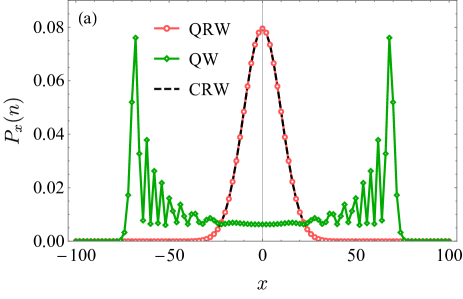
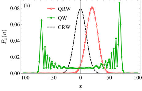
Figure 1: The walker’s position distribution $P_{x}(n)$ as the function of position $x$ for quantum random walk (red square markered line), quantum walk (green circle markered line), classical walk (black-dashed line). The total step number is chosen as $n=100$ , and we only plot the probability at the even lattice since the probability at the odd lattice is zero. The classical random walk is given as an symmetric binomial distribution, which follows from Eq. (13) with $p_{1}=p_{-1}=0.5$. (a) The coin initial state is chosen as $p_{1}=p_{-1}=0.5,\,\eta=0$. The walker’s position distribution of the quantum random walk returns to the one of the classical random walk. (b) The coin’s initial state is chosen as $p_{1}=p_{-1}=0.5,\,\eta=0.1$. The initial coherence of the coin leads to asymmetric binomial distribution for the quantum random walk.

As a comparison, we demonstrate the position distribution of QRW, QW and CRW in Fig. 1. The total step number is $n=100$, and we only plot the probability at the even lattice since the probability at the odd lattice is zero. In Fig. 1(a), we consider an initially decoherenced coin state with $p_{1}=p_{-1}=0.5,\,\eta=0$. The position distribution of QRW (red square marked line) returns to the one of CRW (black dashed line) while the position distribution of QW is ballistic (green circle marked line). In Fig. 1(b), we choose the initial state with coherence by setting $p_{1}=p_{-1}=0.5,\,\eta=0.1$. The positive non-diagonal term of the density matrix results in the right-hand movement for the QRW, namely, the coherence of the coin induces the asymmetry in the corresponding position distribution.

With the position distribution given by Eq. (36), we obtain the expectation and the variance of the walker’s position after $n$ steps, according to Eqs. (14) and (15), as

$$\left\langle x\right\rangle=2n\mathrm{Re}\eta,$$ (37)

and

$$\left\langle\Delta x^{2}\right\rangle=n\left[1-\left(2\mathrm{Re}\eta\right)^{2}\right],$$ (38)

respectively. The above two relations of Eqs. (37) and (38) are the main results of this paper, which show that the coherence in the initial coin state results in the directional moving of the walker.

IV The correlation in quantum walk

In Sec. II and III, we have discussed the position distribution in CRW and QRW, and demonstrate that no correlation exists in CRW and QRW between different steps. In this section, we will show that the correlation indeed exists between different steps in QW, which is qualified through the convariance of the coin state between the initial time and final time.

In QW, the walker has only one coin, and the one-step evolution is described by Eq. (3) with the same transition process as in CRW. Different from CRW, the flipping process in QW is substituted by a unitary evolution $\mathscr{C}\left(\rho\right)=C\rho C^{\dagger}$ with the Hadamard matrix

$$C=\frac{1}{\sqrt{2}}\left(\begin{array}[]{cc}1&1\\ 1&-1\end{array}\right)$$ (39)

operating on the coin state.

The density matrix of the walker and coin after $n$ steps follows from Eq. 3 as

$$\rho(n)=(TC)^{n}\rho(0)(TC)^{\dagger n}.$$ (40)

The transition operator $T$ is defined in Eq. (9), and the initial state $\rho(0)$ is given as Eq. (2). To describe the coin’s distribution after $n$ steps, we perform a measurement of the Pauli operator $\sigma_{z}$ on the coin, as $\sigma_{z}\left|\pm 1\right\rangle_{c}=\pm\left|\pm 1\right\rangle_{c}$. The expectation of $\sigma_{z}$ after $n$ steps is

$$\left\langle\sigma_{z}(n)\right\rangle=\mathrm{Tr}\left[\sigma_{z}\rho_{c}(n)\right],$$ (41)

where $\rho_{c}(n)$ is the reduced density matrix of the coin after $n$ steps. To figure out the correlation between the initial time and final time, we perform a joint measurement of $\sigma_{z}$ at the initial time.and after $n$ steps, the expectation $\left\langle\sigma_{z}(n)\sigma_{z}(0)\right\rangle$ follows

$$\left\langle\sigma_{z}(n)\sigma_{z}(0)\right\rangle=\sum_{\nu_{1},\nu_{2}=\pm 1}\nu_{1}\nu_{2}\mathrm{Tr}\left[E_{\nu_{2}}U(n)E_{\nu_{1}}\rho(0)E_{\nu_{1}}U^{\dagger}(n)E_{\nu_{2}}\right],$$ (42)

where $\nu_{1}$($\nu_{2}$) gives the measurement result at the initial time (after $n$ steps), and $E_{\nu_{\alpha}}=\left|\nu_{\alpha}\right\rangle_{c}\left\langle\nu_{\alpha}\right|,\alpha=1,2$ is the projection operator. Note that the non-diagonal term of $\rho(0)$ vanishes in the initial measurement, i.e.

$$E_{\nu_{1}}\rho(0)E_{\nu_{1}}=\left|0\right\rangle_{w}\left\langle 0\right|\otimes p_{\nu_{1}}^{(0)}\left|\nu_{1}\right\rangle_{c}\left\langle\nu_{1}\right|.$$ (43)

Hence, we only need to consider for the diagonal initial state without coherence. The correlation in the coin is described by the covariance

$$\left\langle\Delta\left[\sigma_{z}(n)\sigma_{z}(0)\right]\right\rangle=\left\langle\sigma_{z}(n)\sigma_{z}(0)\right\rangle-\left\langle\sigma_{z}(n)\right\rangle\left\langle\sigma_{z}(0)\right\rangle,$$ (44)

which is obtained explicitly as (detailed derivation in Appendix A)

$$\left\langle\Delta\left[\sigma_{z}(n)\sigma_{z}(0)\right]\right\rangle=\left(1-\frac{\sqrt{2}}{2}+\frac{\left(-1\right)^{n}}{2\pi}\int_{-\pi}^{\pi}\left(\frac{\cos\left(2\omega_{k}n\right)}{1+\left(\cos k\right)^{2}}\right)\mathrm{d}k\right)\left[1-\left(p_{1}^{(0)}-p_{-1}^{(0)}\right)^{2}\right],$$ (45)

with $\omega_{k}=\arcsin\left(\sin k/\sqrt{2}\right).$ In the large $n$ limit ($n\rightarrow\infty$), the integral in Eq. (45) diminishes due to the highly oscillated term $\cos\left(2\omega_{k}n\right)$, so that the covariance approaches a constant

$$\lim_{n\rightarrow\infty}\left\langle\Delta\left[\sigma_{z}(n)\sigma_{z}(0)\right]\right\rangle=\left(1-\frac{\sqrt{2}}{2}\right)\left[1-\left(p_{1}^{(0)}-p_{-1}^{(0)}\right)^{2}\right].$$ (46)

The non-zero covariance suggests that the correlation generates through the coin’s flipping process, where the final coin state is correlated to the initial coin state.

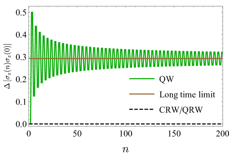
Figure 2: (a) The covariance $\left\langle\Delta\left[\sigma_{z}(n)\sigma_{z}(0)\right]\right\rangle$ varies with different steps. The initial coin density matrix is chosen as the maximal mixed state, and the coin operator is chosen as the Hadamard matrix. The Green curve gives the covariance for quantum walk by Eq. (45), while the horizontal dashed line gives the covariance for classical random walk and quantum random walk. The brown horizontal solid line shows the covariance approaches to the constant $1-\sqrt{2}/2$, as predicted by Eq. (46) at large $n$ limit.

In Fig. 2, we illustrate the covariance $\left\langle\Delta\left[\sigma_{z}(n)\sigma_{z}(0)\right]\right\rangle$ of QW, QRW, and CRW, where the initial coin is chosen as the maximally mixed state with $p_{1}^{(0)}=p_{-1}^{(0)}=0.5$. It is clearly seen in Fig. 2 that the covariance of QW (Green curve), given by Eq. (45), oscillates with the increasing of $n$, and gradually converges to a non-zero constant $1-1/\sqrt{2}$ (the brown horizontal line), which is consistent with the analytical result of Eq. (46).

The non-zero covariance implies the coin state after $n$ steps is correlated to the initial coin state, as shown in Tab. 1, which implies that the coin will remember its initial state for no matter how many steps the walker moves. The covariance of CRW and QRW is both zero (the dashed horizontal line). In CRW, we have $\left\langle\sigma_{z}(n)\sigma_{z}(0)\right\rangle=\left\langle\sigma_{z}(n)\right\rangle\left\langle\sigma_{z}(0)\right\rangle$ which leads the corresponding covariance equals zero, and indicates the flipping process at each step is independent. In QRW, the flipping process for different coins at different steps is independent, and thus the covariance of QRW $\left\langle\Delta\sigma_{z}^{n}(n)\sigma_{z}^{1}(0)\right\rangle=\left\langle\sigma_{z}^{n}(n)\sigma_{z}^{1}(0)\right\rangle-\left\langle\sigma_{z}^{n}(n)\right\rangle\left\langle\sigma_{z}^{1}(0)\right\rangle$ is also zero, where $\sigma_{z}^{1}(0)$ measures the state for the first coin before walking, and $\sigma_{z}^{n}(n)$ measures the state of the $n$-th coin after $n$ steps. Therefore, we state that no correlation exists between different steps in CRW and QRW, while strong correlation exists in QW.

V quantum random walk in 2D lattice

With the theoretical framework of one-dimensional quantum random walk established in Sec. III, it is convenient for us to discuss QRW in two-dimensional lattice. Interestingly, unlike the 1D QRW, in the 2D case, the influence of the coherence in the coin’s initial state on the position distribution of the the walker is more complicated, as demonstrated in this section.

For QRW in 2D lattice, the Hilbert space of the walker is expanded as $\left\{\left|\vec{r}\right\rangle|\,\vec{r}=\left(x,y\right),x,y\in Z\right\}$. And the Hilbert for each coin space is four dimension $\left\{\left|\vec{u}\right\rangle\left|\text{$\vec{u}$=$\vec{R},\,\vec{L},\,\vec{U},\,\vec{D}$}\right.\right\}$, to determine the walker moves right $\vec{R}=(1,0)$, left $\vec{L}=(-1,0)$, up $\vec{U}=(0,1)$, and down $\vec{D}=(0,-1)$ correspondingly. We still consider the walker initially stays at the origin of the coordinates $\left|(0,0)\right\rangle_{w}$, and has many coins prepared in the same initial state. In this situation, the initial density matrix for the walker and the coins follows

$$\rho(0)=\left|(0,0)\right\rangle_{w}\left\langle(0,0)\right|\otimes\bigotimes_{l=1}^{n}\rho_{l,c},$$ (47)

where $\rho_{l,c}$ is the density matrix of the $l$-th coin, and can be represented by a general non-negative $4\times 4$ Hermite matrix as

$$\rho_{k,c}=\left(\begin{array}[]{cccc}q_{1}&\eta_{12}&\eta_{13}&\eta_{14}\\ \eta_{21}&q_{2}&\eta_{23}&\eta_{24}\\ \eta_{31}&\eta_{32}&q_{3}&\eta_{34}\\ \eta_{41}&\eta_{42}&\eta_{43}&q_{4}\end{array}\right),$$ (48)

The coin flipping process and the transition process are the same as that described by Eq. (25) and Eq. (20). The coin operator $C_{l}$ is also given by Eq. (26), where $\tilde{C}_{l}$ can be chosen as a general U(4) matrix. We consider the Grover coin acting on the $l$-th coin (Grover, 1997; Shenvi et al., 2003), i.e.

$$\tilde{C}_{l}=\frac{1}{2}\left(\begin{array}[]{cccc}-1&1&1&1\\ 1&-1&1&1\\ 1&1&-1&1\\ 1&1&1&-1\end{array}\right).$$ (49)

Analogous to Eq. (20) in the 1D case, the position of walker changes according to the state of the $l$-th coin $\left|\vec{u}\right\rangle_{l}$ with $u=R,L,U,D$. So that, the transition operator for the 2D case reads

$$T_{l}=\sum_{\vec{u}}\sum_{\vec{r}}\left|\vec{r}+\vec{u}\right\rangle_{w}\left\langle\vec{r}\right|\otimes\left|\vec{u}\right\rangle_{l}\left\langle\vec{u}\right|\otimes\bigotimes_{j\neq l}^{n}I_{j},$$ (50)

Similar to the 1D QRW, the position distribution is unique determined by the diagonal elements for the flipped coin $\tilde{\rho}_{l,c}=\mathscr{C}_{l}\left(\rho_{l,c}\right)$, as noted by $\rho_{uu}=\left\langle\vec{u}\right|\tilde{\rho}_{l,c}\left|\vec{u}\right\rangle_{l}$. The probabilities $\left\{\rho_{uu}\right\}$ can be further expressed as

$$\left(\begin{array}[]{c}\rho_{RR}\\ \rho_{LL}\\ \rho_{UU}\\ \rho_{DD}\end{array}\right)=\frac{1}{4}\left(\begin{array}[]{cccc}1&-2&-2&-2\\ 1&-2&2&2\\ 1&2&-2&2\\ 1&2&2&-2\end{array}\right)\left(\begin{array}[]{c}1\\ \zeta_{1}\\ \zeta_{2}\\ \zeta_{3}\end{array}\right)$$ (51)

with

$$\zeta_{1} =\textrm{Re}\left(\eta_{12}\right)-\textrm{Re}\left(\eta_{34}\right)$$ (52)

$$\zeta_{2} =\textrm{Re}\left(\eta_{13}\right)-\textrm{Re}\left(\eta_{24}\right)$$ (53)

$$\zeta_{3} =\textrm{Re}\left(\eta_{14}\right)-\textrm{Re}\left(\eta_{23}\right).$$ (54)

Here, $\left\{\zeta_{i}|i=1,2,3\right\}$ is named the effective coherence, and is determined by the difference of the real part of the non-diagonal terms of the coin density matrix of Eq. (48)

In this case, the final position distribution of the walker follows (See Appendix for detailed derivation)

$$P_{(x,y)}(n)=\sum_{j}\Upsilon_{j}\left(x,y,n\right)\rho_{RR}^{\frac{j+x}{2}}\rho_{LL}^{\frac{j-x}{2}}\rho_{UU}^{\frac{n-j+y}{2}}\rho_{DD}^{\frac{n-j-y}{2}},$$ (55)

where

$$\Upsilon_{j}\left(x,y,n\right)=\left(\begin{array}[]{c}n\\ j\end{array}\right)\left(\begin{array}[]{c}j\\ \frac{l+x}{2}\end{array}\right)\left(\begin{array}[]{c}n-j\\ \frac{n-l+y}{2}\end{array}\right).$$ (56)

This is a quadrinomial distribution. Note that the summation here has a restriction on $l$, that is, $l+x$ and $n-l+y$ must be even. For those points $(x,y)$ not satisfied this restriction, the probability is zero. The non-negative condition for the density matrix requires that $\rho_{uu}$ are all non-negative, thus, there exists a limitation for the non-diagonal terms or $\left\{\zeta_{i}\right\}$. The allowed values for $\left\{\zeta_{i}\right\}$ is limited in a regular tetrahedron, as illustrate in Fig. 3.

When $\zeta_{i}=0,\,i=1,2,3$, the position distribution of the walker for QRW in 2D lattice is symmetric with $\rho_{uu}=0.25,u=R,L,U,D$, as shown in Fig. 4(a) and (b). We also illustrate the walker’s position distribution with different $\left\{\eta_{ij}\right\}$ in Fig. 4, where the various patterns show the diverse behavior of the QRW in 2D lattice. In the simulation, the total step number is set as $n=40$, the diagonal terms in the coin’s initial density matrix are chosen as $q_{1}=q_{2}=q_{3}=q_{4}=0.25$, the non-diagonal term $\eta_{ij}$ is set as different values in the eight sub-figures.

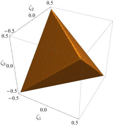
Figure 3: The limitation on $\zeta_{i}$, where the space is expanded by $\zeta_{1}$, $\zeta_{2}$, and $\zeta_{3}$. The allowed region for $\left\{\zeta_{i}\right\}$ is surrounded by the orange regular tetrahedrons obtained from the inequalities $\rho_{RR}\geq 0,\,\rho_{LL}\geq 0,\,\rho_{UU}\geq 0,\,\rho_{DD}\geq 0$ with Eq. (51).

Then we focus on the expectation and the variance of the walker’s position. Since each step is independent for the quadrinomial distribution, the expectation of the walker’s position follows from Eq. (55) as (detailed derivation in the Appendix V)

$$\left\langle\vec{r}\right\rangle =n(-\zeta_{2}-\zeta_{3},-\zeta_{2}+\zeta_{3}),$$ (57)

The variances of the walker’s position along the $x$ and $y$ direction are

$$\left\langle\Delta x^{2}\right\rangle =n[\frac{1}{2}-\zeta_{1}-(\zeta_{2}+\zeta_{3})^{2}],$$ (58)

$$\left\langle\Delta y^{2}\right\rangle =n[\frac{1}{2}+\zeta_{1}-(\zeta_{2}-\zeta_{3})^{2}],$$ (59)

respectively. The total variance for $\vec{r}$ is

$$\left\langle\Delta\vec{r}^{2}\right\rangle =n\left(1-2\zeta_{2}^{2}-2\zeta_{3}^{2}\right).$$ (60)

These relations are cheeked by the exact numerical results illustrated in Fig. (4). Equation (57) shows that only $\zeta_{2}$ and $\zeta_{3}$ determine the orientation at $x$ or $y$, while $\zeta_{1}$ does not. According to Eq. (51), $p_{x}=p_{LL}+p_{RR}=1/2-$$\zeta_{1}$, namely, $\zeta_{1}$ only determines the probability that the walker moves along $x$ or $y$ direction. Different from 1D case, where the non-zero $\eta$ leads to orientation of the walker, in 2D case, the effect of the coherence might cancel with each other for some suitable $\eta_{ij}$ that makes the effective coherence $\zeta_{i}=0$, as shown in Eqs. (52), (53), and (54). This prediction is verified with an numerical example shown in Fig. 4(b), where the walker’s position follows symmetric distribution with non-zero $\eta_{ij}$. The above discovery reveals a fascinating feature of QRW in 2D lattice: even the coherence exists in the coin’s initial state, the walker may not perform directional walking.

When the probabilities $\rho_{UU}=\rho_{DD}=0$ ($\rho_{LL}=\rho_{RR}=0$), the walker moves only along the $x$ ($y$) direction, in which situation the coherence satisfies $\zeta_{1}=-1/2,\,\zeta_{2}=\zeta_{3}$ ( $\zeta_{1}=1/2,\,\zeta_{2}=-\zeta_{3}$ ). The orientation is then only determined by the effective coherence $\zeta_{3}$, and thus the QRW in 2D lattice in this case returns to the 1D QRW, as demonstrated in Fig. 4(c) (Fig. 4(d)).

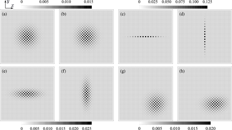
Figure 4: The walker’s position distribution $P_{(x,y)}(n)$ as the function of space location in quantum random walk in 2D lattice. Here, the total step number is set as $n=40$, and the diagonal terms in the coin’s initial density matrix are chosen as $q_{1}=q_{2}=q_{3}=q_{4}=0.25$. The subfigures are divided into four groups, $\left\{\textrm{(a),(b)}\right\}$, $\left\{\textrm{(c),(d)}\right\}$, $\left\{\textrm{(e),(f)}\right\}$, and $\left\{\textrm{(g),(h)}\right\}$. In each group, the two sub-figures share the same plot-bar. (a) All the $\eta_{ij}$ equals zero ($\zeta_{1}=\zeta_{2}=\zeta_{3}=0$). (b) All $\eta_{ij}=0.25$, and the effect coherence diminishes ($\zeta_{1}=\zeta_{2}=\zeta_{3}=0$). (c) Only $\eta_{12}=\eta_{21}=-\eta_{34}=-\eta_{43}=-0.25$, the others $\eta_{ij}$ equals zero ($\zeta_{1}=-0.5,\zeta_{2}=\zeta_{3}=0$). (d) $\eta_{12}=\eta_{21}=-\eta_{34}=-\eta_{43}=0.25$ , the others $\eta_{ij}$ equals zero ($\zeta_{1}=0.5,\zeta_{2}=\zeta_{3}=0$). (e) $\eta_{12}=\eta_{21}=-\eta_{34}=-\eta_{43}=-0.2$, the others $\eta_{ij}$ equals zero ($\zeta_{1}=-0.4,\zeta_{2}=\zeta_{3}=0$). (f) $\eta_{12}=\eta_{21}=-\eta_{34}=-\eta_{43}=0.2$, the others $\eta_{ij}$ equals zero ($\zeta_{1}=0.4,\zeta_{2}=\zeta_{3}=0$). (g) $\eta_{14}=\eta_{41}=-\eta_{23}=-\eta_{32}=-0.1$, the others $\eta_{ij}$ equals zero ($\zeta_{3}=-0.2,\zeta_{1}=\zeta_{2}=0$). (h) $\eta_{12}=\eta_{21}=-\eta_{34}=-\eta_{43}=-0.1$, and $\eta_{23}=\eta_{32}=0.2$, the others $\eta_{ij}$ equals zero ($\zeta_{1}=-0.2,\zeta_{2}=0,\zeta_{3}=-0.2$). The expectation and variance of the walker’s position shown in these sub-figures are consistent with the theoretical predictions given by Eqs. (57), (58), and (59).

VI Conclusion and Discussion

In this paper, we extend classical random walk (CRW) to quantum random walk (QRW) via the ensemble interpretation, and clarify the relation between CRW, QRW, and QW (see Tab. 1). QRW is quantum extension of CRW from the ensemble interpretation, while QW is the quantum extension of CRW from the single-coin interpretation.

Observed the difference of the position distribution for CRW/QRW (binomial) and QW (ballistic), we interpret the different position distribution from the correlation aspect. In CRW, the flipping process in each step is independent, and thus no correlation exists between different steps. We obtain a binomial distribution for the walker’s position(van Kampen, 2007). In QRW, the walker flips different coins at different steps. Still no correlation exists, and we retain the binomial distribution. In QW, the sequential unitary evolution engenders strong correlation between each steps. To qualify the correlation between different steps, we calculate the covariance between the initial coin state and final coin state in those walks. The result shows that the covariance is non-zero for QW while zero for CRW/QRW.

It is found that in QRW the walker performs directional walking once the coherence exists in the coin’s initial state. We further prove that, in such case, the stronger the coherence is, the more obvious the directional movement is, and the smaller the fluctuation of the walker’s position distribution is. Besides, QRW in 2D lattice is also studied, where the influence of coin state’s coherence on the walker’s position distribution is found to be more complicated (than that in the 1D case). Different from the one-dimensional case, even if there exists coherence in the coin’s initial state, the walker may not perform directional walking. This is because, under some special conditions, the influence of different non-diagonal terms in the coin’s density matrix on the position distribution of the walker may cancel each other out .

Generally, the main difference of QRW and QW can be understood by the following statement. In QRW, the quantum property refers to the initial coherence of the coin state, which results in a directional walk for the walker. While in QW, the sequential unitary operation on the single coin engenders strong correlation between different steps. This strong correlation results in the non-binomial distribution for the walker’s position.

Appendix A The Covariance for quantum walk

In this section, we derive the the coin’s reduced density matrix and the covariance for QW (Abal et al., 2006). We assume the total system is initially prepared in a pure state

$$\left|\psi_{\pm}(0)\right\rangle=\left|0\right\rangle_{w}\otimes\left|\pm 1\right\rangle_{c},$$ (61)

where $\left|\pm 1\right\rangle_{c}$ describes the initial coin state as $\left|1\right\rangle_{c}=\left(\begin{array}[]{cc}1&0\end{array}\right)^{\mathrm{T}}$, and $\left|-1\right\rangle_{c}=\left(\begin{array}[]{cc}0&1\end{array}\right)^{\mathrm{T}}$. The state after $n$ steps follows

$$\left|\psi_{\pm}(n)\right\rangle=(TC)^{n}\left|\psi_{\pm}(0)\right\rangle,$$ (62)

where $T$ and $C$ is given by Eq. (9) and Eq. (39), respectively. To obtain the reduced density matrix of the coin after $n$ steps, we first represent the initial state in the momentum space as

$$\left|\psi_{\pm}(0)\right\rangle=\frac{1}{\sqrt{2\pi}}\int_{-\pi}^{\pi}\mathrm{d}k\left|k\right\rangle\otimes\left|\pm 1\right\rangle_{c},$$ (63)

where

$$\left|k\right\rangle=\frac{1}{\sqrt{2\pi}}\sum_{x=-\infty}^{\infty}e^{ikx}\left|x\right\rangle_{w}.$$ (64)

In the momentum space, the transition operator of Eq. (9) is rewritten as

$$T=e^{-ik}\otimes\left|1\right\rangle_{c}\left\langle 1\right|+e^{ik}\otimes\left|-1\right\rangle_{c}\left\langle-1\right|,$$ (65)

and the evolution operator of one step follows

$$TC=\frac{1}{\sqrt{2}}\left(\begin{array}[]{cc}e^{-ik}&e^{-ik}\\ e^{ik}&-e^{ik}\end{array}\right).$$ (66)

Combining Eqs. (62), (63), and (66), we obtain the state after $n$ steps

$$\left|\psi_{\pm}(n)\right\rangle=\frac{1}{\sqrt{2\pi}}\int\mathrm{d}k\left|k\right\rangle\otimes\left(\begin{array}[]{c}\alpha_{k}^{(\pm)}(n)\\ \beta_{k}^{(\pm)}(n)\end{array}\right),$$ (67)

where

$$\alpha_{k}^{(+)}(n) =\frac{1}{2}\left(\kappa_{k}^{(+)}(n)+\frac{\cos k}{\sqrt{1+\left(\cos k\right)^{2}}}\kappa_{k}^{(-)}(n)\right),$$ (68)

$$\alpha_{k}^{(-)}(n) =\frac{e^{-ik}}{2\sqrt{1+\left(\cos k\right)^{2}}}\kappa_{k}^{(-)}(n),$$ (69)

$$\beta_{k}^{(+)}(n) =\frac{e^{ik}}{2\sqrt{1+\left(\cos k\right)^{2}}}\kappa_{k}^{(-)}(n),$$ (70)

$$\beta_{k}^{(-)}(n) =\frac{1}{2}\left(\kappa_{k}^{(+)}(n)-\frac{\cos k}{\sqrt{1+\left(\cos k\right)^{2}}}\kappa_{k}^{(-)}(n)\right),$$ (71)

and

$$\kappa_{k}^{(\pm)}(n)=e^{-in\omega_{k}}\pm\left(-1\right)^{n}e^{in\omega_{k}},$$ (72)

with $\omega_{k}=\arcsin\left(\sin k/\sqrt{2}\right)$. Then, the reduced density matrix of the coin after $n$ steps can be obtained by tracing over the freedom of the walker as,

$$\rho_{c}^{(\pm)}(n)=\mathrm{Tr}_{\mathrm{walker}}\left(\left|\psi_{\pm}(n)\right\rangle\left\langle\psi_{\pm}(n)\right|\right)=\left(\begin{array}[]{cc}\rho_{1,1}^{(\pm)}(n)&\rho_{1,-1}^{(\pm)}(n)\\ \rho_{-1,1}^{(\pm)}(n)&\rho_{-1,-1}^{(\pm)}(n)\end{array}\right),$$ (73)

which is further written as

$$\rho_{c}^{(\pm)}(n)=\left(\begin{array}[]{cc}\frac{1}{2\pi}\int_{-\pi}^{\pi}\left|\alpha_{k}^{(\pm)}(n)\right|^{2}\mathrm{d}k&\frac{1}{2\pi}\int_{-\pi}^{\pi}\alpha_{k}^{(\pm)}(n)\left(\beta_{k}^{(\pm)}(n)\right)^{*}\mathrm{d}k\\ \frac{1}{2\pi}\int_{-\pi}^{\pi}\beta_{k}^{(\pm)}(n)\left(\alpha_{k}^{(\pm)}(n)\right)^{*}\mathrm{d}k&1-\frac{1}{2\pi}\int_{-\pi}^{\pi}\left|\alpha_{p}^{(\pm)}(n)\right|^{2}\mathrm{d}k\end{array}\right).$$ (74)

Combining Eqs. (68-72), we obtain the explicit result for the elements of the reduced matrix as

$$\rho_{1,1}^{(+)}(n) =1-\frac{\sqrt{2}}{4}+\frac{\left(-1\right)^{n}}{4\pi}\int_{-\pi}^{\pi}\left(\frac{\cos\left(2\omega_{k}n\right)}{1+\left(\cos k\right)^{2}}\right)\mathrm{d}k$$ (75)

$$\rho_{1,-1}^{(+)}(n) =\frac{2-\sqrt{2}}{4}+\frac{\left(-1\right)^{n}}{4\pi}\int_{-\pi}^{\pi}e^{-ik}\left(\frac{i\sin(2\omega_{k}n)}{\sqrt{1+\left(\cos k\right)^{2}}}-\frac{\cos k\cos\left(2\omega_{k}n\right)}{1+\left(\cos k\right)^{2}}\right)\mathrm{d}k$$ (76)

$$\rho_{-1,1}^{(+)}(n) =\frac{2-\sqrt{2}}{4}+\frac{\left(-1\right)^{n}}{4\pi}\int_{-\pi}^{\pi}e^{ik}\left(\frac{-i\sin(2\omega_{k}n)}{\sqrt{1+\left(\cos k\right)^{2}}}-\frac{\cos k\cos\left(2\omega_{k}n\right)}{1+\left(\cos k\right)^{2}}\right)\mathrm{d}k$$ (77)

$$\rho_{-1,-1}^{(+)}(n) =\frac{\sqrt{2}}{4}-\frac{\left(-1\right)^{n}}{4\pi}\int_{-\pi}^{\pi}\left(\frac{\cos\left(2\omega_{k}n\right)}{1+\left(\cos k\right)^{2}}\right)\mathrm{d}k$$ (78)

and

$$\rho_{1,1}^{(-)}(n) =\frac{\sqrt{2}}{4}-\frac{\left(-1\right)^{n}}{4\pi}\int_{-\pi}^{\pi}\frac{\cos\left(2\omega_{k}n\right)}{\left(1+\left(\cos k\right)^{2}\right)}\mathrm{d}k$$ (79)

$$\rho_{1,-1}^{(-)}(n) =-\frac{2-\sqrt{2}}{4}+\frac{\left(-1\right)^{n}}{4\pi}\int_{-\pi}^{\pi}e^{-ik}\left(-\frac{i\sin(2n\omega_{k})}{\sqrt{1+\left(\cos k\right)^{2}}}+\frac{\cos k\cos\left(2\omega_{k}n\right)}{1+\left(\cos k\right)^{2}}\right)\mathrm{d}k$$ (80)

$$\rho_{-1,1}^{(-)}(n) =-\frac{2-\sqrt{2}}{4}+\frac{\left(-1\right)^{n}}{4\pi}\int_{-\pi}^{\pi}e^{ik}\left(\frac{i\sin(2n\omega_{k})}{\sqrt{1+\left(\cos k\right)^{2}}}+\frac{\cos k\cos\left(2\omega_{k}n\right)}{1+\left(\cos k\right)^{2}}\right)\mathrm{d}k$$ (81)

$$\rho_{-1,-1}^{(-)}(n) =1-\frac{\sqrt{2}}{4}+\frac{\left(-1\right)^{n}}{4\pi}\int_{-\pi}^{\pi}\left(\frac{\cos\left(2\omega_{k}n\right)}{1+\left(\cos k\right)^{2}}\right)\mathrm{d}k$$ (82)

Then, the expectation by Eq. (42) is obtained from the reduced density matrix as

$$\left\langle\sigma_{z}(n)\sigma_{z}(0)\right\rangle =p_{1}\rho_{1,1}^{(+)}(n)+p_{-1}\rho_{-1,-1}^{(-)}(n)-p_{1}\rho_{-1,-1}^{(+)}(n)-p_{-1}\rho_{1,1}^{(-)}(n)$$ (83)

which is explicitly written as

$$\left\langle\sigma_{z}(n)\sigma_{z}(0)\right\rangle=1-\frac{\sqrt{2}}{2}+\frac{\left(-1\right)^{n}}{2\pi}\int_{-\pi}^{\pi}\left(\frac{\cos\left(2\omega_{k}n\right)}{1+\left(\cos k\right)^{2}}\right)\mathrm{d}k,$$ (84)

The expectations for $\sigma_{z}$ at the initial time and after $n$ steps are $\left\langle\sigma_{z}(0)\right\rangle=p_{1}-p_{-1}$ and

$$\left\langle\sigma_{z}(n)\right\rangle=\left(p_{1}-p_{-1}\right)\left(1-\frac{\sqrt{2}}{2}+\frac{\left(-1\right)^{n}}{2\pi}\int_{-\pi}^{\pi}\left(\frac{\cos\left(2\omega_{k}n\right)}{1+\left(\cos k\right)^{2}}\right)\mathrm{d}k\right),$$ (85)

respectively. Therefore we obtain the covariance of Eq. (45) in the main text. Specially, in the large $n$ limit, the integral in Eqs. (75-82) diminishes due to the highly oscillated term $\cos\left(2\omega_{k}n\right)$ or $\sin\left(2\omega_{k}n\right)$. Therefore, the reduced density matrix of the coin approaches to a constant as

$$\lim_{n\rightarrow\infty}\rho_{c}^{(+)}(n)=\frac{1}{4}\left(\begin{array}[]{cc}4-\sqrt{2}&2-\sqrt{2}\\ 2-\sqrt{2}&\sqrt{2}\end{array}\right),\>\lim_{n\rightarrow\infty}\rho_{c}^{(-)}(n)=\frac{1}{4}\left(\begin{array}[]{cc}\sqrt{2}&-2+\sqrt{2}\\ -2+\sqrt{2}&4-\sqrt{2}\end{array}\right).$$ (86)

This indicates that $\left\langle\sigma_{z}(n)\sigma_{z}(0)\right\rangle$ of Eq. (83) is a constant in the large $n$ limit, which explain why the covariance converges to a constant for $n\rightarrow\infty$, as shown by Eq. (46) in the main text.

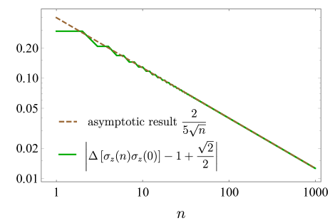
Figure 5: The Log-log plot of the absolute difference of the covariance $\left\langle\Delta\left[\sigma_{z}(n)\sigma_{z}(0)\right]\right\rangle$ and the constant $1-\sqrt{2}/2$. The brown dashed line clearly shows the absolute difference diminishes inverse proportional to $\sqrt{n}$ for large $n$.

To convince that the variance approaches to the constant $1-\sqrt{2}/2$ at long time limit, we show the absolute difference $\left|\left\langle\Delta\left[\sigma_{z}(n)\sigma_{z}(0)\right]\right\rangle-1+\sqrt{2}/2\right|$ in Fig. 5. The green line clearly shows that the absolute difference approaches to zero for long time limit with large $n$ (the brown dashed line). By fitting the exact result of the absolute difference, we obtain the asymptotic result (the brown dashed line)

$$\left|\left\langle\Delta\left[\sigma_{z}(n)\sigma_{z}(0)\right]\right\rangle-1+\sqrt{2}/2\right|\approx\frac{2}{5\sqrt{n}},$$ (87)

which matches well for large $n$.

Appendix B Quantum Random Walk in 2D Lattice

In this appendix, we give the detailed derivation of the walker’s position distribution and the corresponding expectation and variance for QRW in 2D lattice. Similar to Eq. (33), by acting all the coin operator first, we obtain the density matrix after $n$ step as

$$\rho(n)=\sum_{\left\{u_{l},v_{l}\right\}}\left|\sum_{l=1}^{n}\vec{u}_{l}\right\rangle\left\langle\sum_{l=1}^{n}\vec{v}_{l}\right|\otimes\bigotimes_{l=1}^{n}\rho_{u_{l}v_{l}}\left|\vec{u}_{l}\right\rangle_{l}\left\langle\vec{v}_{l}\right|,$$ (88)

where $u_{l}$($v_{l}$)$\in\{(1,0),\,(-1,0),\,(0,1),\,(0,-1)\}$ determines the corresponding direction $R,L,U,D$ . Tracing over the coin Hilbert space, we obtain the probability of a given path $\left\{u_{l}|,l=1,2,...,n\right\}$ as $P_{\left\{u_{l}\right\}}=\prod_{l=1}^{n}\rho_{u_{l}u_{l}}$. The probability for the walker arriving at the position $(x,y)$ after $n$ steps is calculated with the limitation on the path

$$P_{(x,y)}(n)=\sum_{\{u_{l}\}:\sum_{l}\vec{u}_{l}=(x,y)}\prod_{l=1}^{n}\rho_{u_{l}u_{l}}.$$ (89)

If the direction $\vec{u}_{l}=(1,0),\,(-1,0),\,(0,1),\,\mathrm{and}\,(0,-1)$ is chosen for $j,\,l-j,\,m,\,$and $n-l-m$ times respectively, the final position of the walker is $(2j-l,2m-n+l)$. The probability for this event is quadrinomial distributed as

$$P_{[j,l-j,m,n-l-m]}(n)=\left(\begin{array}[]{c}n\\ l\end{array}\right)\left(\begin{array}[]{c}l\\ j\end{array}\right)\left(\begin{array}[]{c}n-l\\ m\end{array}\right)\rho_{RR}^{j}\rho_{LL}^{l-j}\rho_{UU}^{m}\rho_{DD}^{n-l-m}.$$ (90)

The product of the combination number $n!/[j!(l-j)!m!(n-l-m)!]$ gives the number to divide $n$ into four group as $j,\,l-j,\,m,\,$and $n-l-m$ . By setting the final position of the walker as $(2j-l,2m-n+l)=(x,y)$, we can re-express $j$ and $m$ as $j=(x+l)/2$ and $m=(y+n-l)/2$ respectively. Here $j$ and $m$ need to be positive integers, which requires the same parity for the $x$ and $y+n$. Then one can obtain the walker’s position distribution of QRW in 2D lattice as given by Eq. (55). The summation comes from the multiple choice of $l$ leading to the same position $(x,y)$.

Next, we derive the expected position given in Eq. (57) and the variance of the position given in Eq. (60). For the quadrinomial distribution, we can divide the final position shift into each step for the independence of each step, and this results in a classical probability for a summation of independent random variable $\vec{R}(n)=\sum_{l=1}^{n}\vec{R}_{l}.$ Here, $\vec{R}_{l}=\left(X_{l},Y_{l}\right)$ is a two-component random variable which follows the independent identical distribution and takes the value $(1,0),\,(-1,0),\,(0,1)$, and $(0,-1)$ with the probability $\rho_{RR},\,\rho_{LL},\,\rho_{UU}$, and $\rho_{DD}$ respectively. Then, the expectation for $\vec{R}_{l}$ is calculated as

$$\left\langle\vec{R}_{l}\right\rangle=\rho_{RR}(1,0)+\rho_{LL}(-1,0)+\rho_{UU}(0,1)+\rho_{DD}(0,-1)=(\rho_{RR}-\rho_{LL},\rho_{UU}-\rho_{DD}),$$ (91)

and the variances for the components $X_{l}$ and $Y_{l}$ are obtained as

$$\left\langle\Delta X_{l}^{2}\right\rangle=\rho_{RR}+\rho_{LL}-(\rho_{RR}-\rho_{LL})^{2},\>\left\langle\Delta Y_{l}^{2}\right\rangle=\rho_{UU}+\rho_{DD}-(\rho_{UU}-\rho_{DD})^{2}.$$ (92)

respectively. Thus, the variance for $\vec{R}_{l}$ follows as

$$\left\langle\Delta\vec{R}_{l}^{2}\right\rangle=\left\langle\Delta X_{l}^{2}\right\rangle+\left\langle\Delta Y_{l}^{2}\right\rangle=1-(\rho_{RR}-\rho_{LL})^{2}-(\rho_{UU}-\rho_{DD})^{2}.$$ (93)

These results can be further simplified, with the help of Eq. (51), as

$$\left\langle\Delta X_{l}^{2}\right\rangle=\frac{1}{2}-\zeta_{1}-(\zeta_{2}+\zeta_{3})^{2},\>\left\langle\Delta Y_{l}^{2}\right\rangle=\frac{1}{2}+\zeta_{1}-(\zeta_{2}-\zeta_{3})^{2},$$

and

$$\left\langle\vec{R}_{l}\right\rangle=(-\zeta_{2}-\zeta_{3},-\zeta_{2}+\zeta_{3}),\>\left\langle\Delta\vec{R}_{l}^{2}\right\rangle=1-2\zeta_{2}^{2}-2\zeta_{3}^{2}$$

The expectation and variance for the walker’s postion after $n$ steps are thus $\left\langle\vec{r}\right\rangle=n\left\langle\vec{R}_{l}\right\rangle,$ $\left\langle\Delta x^{2}\right\rangle=n\left\langle\Delta X_{l}^{2}\right\rangle,$ $\left\langle\Delta r^{2}\right\rangle=n\left\langle\Delta Y_{l}^{2}\right\rangle$ and $\left\langle\Delta\vec{r}^{2}\right\rangle=n\left\langle\Delta\vec{R}_{l}^{2}\right\rangle$, which are given explicitly as Eqs. (57) and (60) in the main text.