h KA-TP-15-2019
h IFIRSE-TH-2019-3
One-Loop Corrections to the Two-Body Decays of the Neutral Higgs Bosons in the Complex NMSSM

Abstract

Since no direct signs of new physics have been observed so far indirect searches in the Higgs sector have become increasingly important. With the discovered Higgs boson behaving very Standard Model (SM)-like, however, indirect new physics manifestations are in general expected to be small. On the theory side, this makes precision predictions for the Higgs parameters and observables indispensable. In this paper, we provide in the framework of the CP-violating Next-to-Minimal Supersymmetric extension of the SM (NMSSM) the complete next-to-leading order (SUSY-)electroweak corrections to the neutral Higgs boson decays that are on-shell and non-loop induced. Together with the also provided SUSY-QCD corrections to colored final states, they are implemented in the Fortran code NMSSMCALC which already includes the state-of-the art QCD corrections. The new code is called NMSSMCALCEW. This way we provide the NMSSM Higgs boson decays and branching ratios at presently highest possible precision and thereby contribute to the endeavor of searching for New Physics at present and future colliders.

1 Introduction

The discovery of a scalar particle by the LHC experiments ATLAS [1] and CMS [2] and the subsequent investigation of its properties revealed a Higgs boson that behaves very Standard Model (SM)-like. Also years after its discovery there are no evidences for new physics from direct searches. In this situation the precise investigation of the Higgs sector plays an important role. Indirect effects of physics beyond the SM (BSM) might show up in the properties of the discovered Higgs boson. With a mass of 125.09 GeV [3] it does not exclude the possibility for the Higgs boson of a supersymmetric (SUSY) extension of the SM, like the minimal (MSSM) or the next-to-minimal (NMSSM) ones. Supersymmetry certainly belongs to the best motivated and most intensively studied BSM extensions, and the NMSSM, with a Higgs sector consisting of seven Higgs bosons arising after electroweak symmetry breaking (EWSB) from the two doublet and singlet fields of the Higgs sector, provides a rich phenomenology [4, 5]. The experimental limits strongly restrict possible new physics effects in the Higgs sector and call for precision in the theory predictions for the Higgs boson observables. This is also necessary in order to be able to distinguish between new physics extensions in case of discovery.

In this paper, we concentrate on the NMSSM Higgs boson decays. While the (SUSY-)QCD corrections can be taken over from the MSSM case with the appropriate modifications and a minimum of effort, this is not the case for the electroweak (EW) corrections. In the recent years there has been some progress on this subject. In the CP-conserving NMSSM, members of our group computed the next-to-leading order (NLO) SUSY-EW and SUSY-QCD corrections to the decays of CP-odd NMSSM Higgs bosons into stop pairs and found that the both the EW and the SUSY-QCD corrections are significant and can be of opposite sign [6]. The authors of [7, 8] provided in the framework of the CP-conserving NMSSM its full one-loop renormalization and the two-body Higgs decays at one-loop order in the on-shell (OS) renormalization scheme. A generic calculation of the two-body partial decays widths at full one-loop level was provided in [9] in the $\overline{\text{DR}}$ scheme. In [10] the full one-loop corrections for the neutral CP-violating NMSSM Higgs bosons were calculated to their decays into fermions and gauge bosons and combined with the leading QCD corrections. For the Higgs-to-Higgs decays, we provided in previous papers the complete one-loop [11] and the order ${\cal O}(\alpha_{t}\alpha_{s})$ two-loop [12] corrections in the CP-conserving and CP-violating NMSSM, respectively.

In this work, we compute, in the framework of the CP-violating NMSSM, the complete next-to-leading order (SUSY-)electroweak corrections to the neutral NMSSM Higgs boson decays into all tree-level induced SM final states, i.e. into fermion and massive gauge boson pairs, but also into non-SM pairs, namely gauge and Higgs boson final states, chargino and neutralino pairs, and into squarks. Where applicable we combine our corrections with the already available (SUSY-)QCD corrections. We furthermore include the complete one-loop corrections to the decays into Higgs boson pairs, cf. Refs. [11, 12]. For the loop-induced decays into gluon and photon pairs as well as a photon and a $Z$ boson no corrections are provided as they would be of two-loop order. For the first time, we present the one-loop corrections to the electroweakino, stop and sbottom masses in the context of the CP-violating NMSSM, by applying both OS and $\overline{\text{DR}}$ schemes. We have implemented our corrections in our original code NMSSMCALC [13], which calculates, based on a mixed OS-$\overline{\text{DR}}$ scheme, the NMSSM Higgs mass corrections and decays in both the CP-conserving and CP-violating case. This way we provide the NMSSM Higgs boson decays and branching ratios at presently highest possible precision including the state-of-the-art (SUSY-)QCD and the computed (SUSY-)EW corrections. In the EW higher-order corrections we not only include the NLO vertex corrections but also take into account the proper on-shell conditions of the external decaying Higgs bosons up to two-loop order ${\cal O}(\alpha_{t}\alpha_{s}+\alpha_{t}^{2})$. This is the order up to which the mass corrections for the NMSSM Higgs bosons both in the CP-conserving [14] and CP-violating case [15, 16, 17] have been implemented in NMSSMCALC. The new program is called NMSSMCALCEW can be obtained at the url: https://www.itp.kit.edu/$\sim$maggie/NMSSMCALCEW/. Here also a detailed description of the program and its structure are given, instructions on how to compile and run it as well as information on modifications, which is constantly updated. A brief description of the code is given in Appendix B.

The paper is organized as follows. In Section 2 we introduce the NMSSM sectors at tree level, that are relevant for our computation, and set our notation before we move on to the NMSSM at one-loop level in Section 3. We here describe the renormalization of the Higgs, chargino/neutralino, and squark sectors as well as the loop corrections to the Higgs boson masses and mixings, to the neutralino and chargino masses, and finally to the squark masses and their mixings. Section 4 is devoted to the detailed presentation of our calculation of the one-loop corrections to the neutral non-loop induced Higgs boson decays into on-shell final states, namely into fermion pairs, massive gauge boson pairs, final states with one gauge and one Higgs boson, neutralino and chargino pairs, and squark final states. In Section 5 we present the numerical analysis of the one-loop corrections to the Higgs boson branching ratios into SM and SUSY final states, where we discuss in particular the size of the newly implemented corrections to both the branching ratios and to the electroweakino and third generation squark masses. Our conclusions are given in Section 6. Explicit expressions of the counterterm couplings for the decays of neutral Higgs bosons into a squark pair are displayed in Appendix A.

2 The NMSSM at Tree Level

We are working in the complex NMSSM with a preserved $\mathbb{Z}_{3}$ symmetry. The Lagrangian of the NMSSM can be divided into the Lagrangian of the MSSM and the additional part coming from the NMSSM. For convenience of the reader and to set our notation, we give here the parts of the Lagrangian that are relevant for our calculations. For the Higgs sector we need the NMSSM Higgs potential. It is derived from the NMSSM superpotential $W_{\text{NMSSM}}$, the corresponding soft SUSY-breaking terms, and the $D$-term contributions. With the Higgs doublet superfields $\hat{H}_{u}$ and $\hat{H}_{d}$ coupling to the up- and down-type quark superfields, respectively, and the singlet superfield $\hat{S}$, we have for the NMSSM superpotential

$$W_{\text{NMSSM}}=W_{\text{MSSM}}-\epsilon_{ab}\lambda\hat{S}\hat{H}_{d}^{a}\hat{H}_{u}^{b}+\frac{1}{3}\kappa\hat{S}^{3}~{},$$ (2.1)

where $a,b=1,2$ are the indices of the fundamental $SU(2)_{L}$ representation and $\epsilon_{ab}$ is the totally antisymmetric tensor with $\epsilon_{12}=\epsilon^{12}=1$ . The MSSM part reads

$$W_{\text{MSSM}}=-\epsilon_{ab}\bigl{(}y_{u}\hat{H}_{u}^{a}\hat{Q}^{b}\hat{U}^{c}-y_{d}\hat{H}_{d}^{a}\hat{Q}^{b}\hat{D}^{c}-y_{e}\hat{H}_{d}^{a}\hat{L}^{b}\hat{E}^{c}\bigr{)}\;,$$ (2.2)

in terms of the left-handed quark and lepton superfield doublets $\hat{Q}$ and $\hat{L}$ and the right-handed up-type, down-type, and electron-type superfield singlets $\hat{U}$, $\hat{D}$, and $\hat{E}$, respectively. Charge conjugation is denoted by the superscript $c$, and color and generation indices have been omitted. The NMSSM superpotential contains the coupling $\kappa$ of the self-interaction of the new singlet superfield and the coupling $\lambda$ for the $\hat{S}$ interaction with the two Higgs doublet superfields. Both couplings are complex. The quark and lepton Yukawa couplings $y_{d},$ $y_{u}$, and $y_{e}$ are in general complex. However, in case of no generation mixing, as assumed in this paper, the phases of the Yukawa couplings can be absorbed through a redefinition of the quark fields, so that the phases can be chosen arbitrarily without changing the physical meaning [18]. The soft SUSY-breaking NMSSM Lagrangian in terms of the component fields $H_{u},H_{d}$ and $S$ reads

$$\mathcal{L}_{\text{NMSSM}}^{\text{soft}}=\mathcal{L}_{\text{MSSM}}^{\text{soft}}-m_{S}^{2}|S|^{2}+(\epsilon_{ab}A_{\lambda}\lambda SH_{d}^{a}H_{u}^{b}-\frac{1}{3}A_{\kappa}\kappa S^{3}+h.c.)\;.$$ (2.3)

It contains two more complex parameters specific to the NMSSM, the soft SUSY-breaking trilinear couplings $A_{\lambda}$ and $A_{\kappa}$. The soft SUSY-breaking MSSM contribution can be cast into the form

$$\mathcal{L}_{\text{MSSM}}^{\text{soft}} =-m_{H_{d}}^{2}|H_{d}|^{2}-m_{H_{u}}^{2}|H_{u}|^{2}-m_{\tilde{Q}}^{2}|\tilde{Q}|^{2}-m_{\tilde{u}_{R}}^{2}|\tilde{u}_{R}|^{2}-m_{\tilde{d}_{R}}^{2}|\tilde{d}_{R}|^{2}-m_{\tilde{L}}^{2}|\tilde{L}|^{2}-m_{\tilde{e}_{R}}^{2}|\tilde{e}_{R}|^{2}$$

$$\quad+\epsilon_{ab}(y_{u}A_{u}H_{u}^{a}\tilde{Q}^{b}\tilde{u}^{*}_{R}-y_{d}A_{d}H_{d}^{a}\tilde{Q}^{b}\tilde{d}^{*}_{R}-y_{e}A_{e}H_{d}^{a}\tilde{Q}^{b}\tilde{e}^{*}_{R}+h.c.)$$

$$\quad-\frac{1}{2}(M_{1}\tilde{B}\tilde{B}+M_{2}\tilde{W}_{i}\tilde{W}_{i}+M_{3}\tilde{G}\tilde{G}+h.c)\;,$$ (2.4)

where the SM-type and SUSY fields corresponding to a superfield (denoted with a hat) are represented by a letter without and with a tilde, respectively. The indices $\tilde{Q}$ ($\tilde{L}$) of the soft SUSY-breaking masses denote, exemplary for the first generation, the left-handed quark (lepton) doublet component fields of the corresponding quark and lepton superfields, and $\tilde{u}_{R},\tilde{d}_{R},\tilde{e}_{R}$ the right-handed component fields for the up-type and down-type quarks, and charged leptons, respectively,. The trilinear couplings $A_{u}$, $A_{d}$ and $A_{e}$ of the up-type and down-type quarks and charged leptons are in general complex, whereas the soft SUSY-breaking mass terms $m_{x}^{2}$ ($x=S,H_{u},H_{d},\tilde{Q},\tilde{u}_{R},\tilde{d}_{R},\tilde{L},\tilde{e}_{R}$) are real. The soft SUSY-breaking mass parameters of the gauginos, $M_{1}$, $M_{2}$, $M_{3}$, for the bino, the winos, and the gluinos, $\tilde{B}$, $\tilde{W}_{i}$ ($i=1,2,3$), and $\tilde{G}$, corresponding to the weak hypercharge $U(1)$, the weak isospin $SU(2)$, and the color $SU(3)$ symmetry, are in general complex. The $R$-symmetry can be exploited to choose either $M_{1}$ or $M_{2}$ to be real. In this paper we keep both $M_{1}$ and $M_{2}$ complex.

Expanding the scalar Higgs fields about their vacuum expectation values (VEVs) $v_{u}$, $v_{d}$, and $v_{s}$, two further phases, $\varphi_{u}$ and $\varphi_{s}$, are introduced which describe the phase differences between the VEVs,

$$H_{d}=\begin{pmatrix}\frac{1}{\sqrt{2}}(v_{d}+h_{d}+ia_{d})\\ h_{d}^{-}\end{pmatrix}~{},\;\;\;H_{u}=e^{i\varphi_{u}}\begin{pmatrix}h_{u}^{+}\\ \frac{1}{\sqrt{2}}(v_{u}+h_{u}+ia_{u})\end{pmatrix}~{},\;\;\;S=\frac{e^{i\varphi_{s}}}{\sqrt{2}}(v_{s}+h_{s}+ia_{s})~{}.$$ (2.5)

For vanishing phases, the fields $h_{i}$ and $a_{i}$ with $i=d,u,s$ correspond to the CP-even and CP-odd part of the neutral entries of $H_{d}$, $H_{u}$ and $S$. The charged components are denoted by $h_{d,u}^{\pm}$. In this paper, we set the phases of the Yukawa couplings to zero. We furthermore re-phase the left- and right-handed up-quark fields as $u_{L}\to e^{-i\varphi_{u}}u_{L}$ and $u_{R}\to e^{i\varphi_{u}}u_{R}$, so that the quark and lepton mass terms yield real masses.

After electroweak symmetry breaking (EWSB) the six Higgs interaction states mix and in the basis $\phi=(h_{d},h_{u},h_{s},a_{d},a_{u},a_{s})$ the mass term is given by

$${\cal L}^{m}_{\text{neutral}}=\frac{1}{2}\phi^{T}M_{\phi\phi}\phi\;.$$ (2.6)

The mass matrix $M_{\phi\phi}$ is obtained from the second derivative of the Higgs potential with respect to the Higgs fields in the vacuum. The explicit expression of the mass matrix $M_{\phi\phi}$ can be found in Ref. [15]. The transformation into mass eigenstates at tree level can be performed with orthogonal matrices $\mathcal{R},\mathcal{R}^{G}$,

$${\text{diag}}(m_{h_{1}}^{2},m_{h_{2}}^{2},m_{h_{3}}^{2},m_{h_{4}}^{2},m_{h_{5}}^{2},0) = \mathcal{R}\mathcal{R}^{G}M\left(\mathcal{R}\mathcal{R}^{G}\right)^{T},$$ (2.7)

$$(h_{1},h_{2},h_{3},h_{4},h_{5},G)^{T} = \mathcal{R}\mathcal{R}^{G}(h_{d},h_{u},h_{s},a_{d},a_{u},a_{s})^{T}$$ (2.8)

$$= {\cal R}(h_{d},h_{u},h_{s},a,a_{s},G)^{T}\;,$$

where the matrix $\mathcal{R}^{G}$ is used first to single out the Goldstone boson $G$. The tree-level Higgs mass eigenstates are denoted by the small letter $h$, and their masses are ordered as $m_{h_{1}}\leq...\leq m_{h_{5}}$.

The mass term for the charged components of the Higgs doublets in

$${\cal L}^{m}_{\text{charged}}=\begin{pmatrix}h_{d}^{+},h_{u}^{+}\end{pmatrix}M_{h^{+}h^{+}}\begin{pmatrix}h_{d}^{-}\\ h_{u}^{-}\end{pmatrix},$$ (2.9)

is given by

$$M_{h^{+}h^{+}}=\frac{1}{2}\begin{pmatrix}{t_{\beta}}&1\\ 1&1/{t_{\beta}}\end{pmatrix}\bigg{[} M_{W}^{2}s_{2\beta}+\frac{\lvert\lambda\rvert v_{s}}{\cos(\varphi_{\lambda}+\varphi_{u}+\varphi_{s})}\left(\sqrt{2}\,\text{Re}\,A_{\lambda}+\lvert\kappa\rvert v_{s}\cos(\varphi_{\kappa}+3\varphi_{s})\right)$$

$$-\frac{2|\lambda|^{2}M_{W}^{2}s_{\theta_{W}}^{2}}{e^{2}}s_{2\beta}\bigg{]}\;,$$ (2.10)

where $M_{W}$ is the mass of the $W$ boson, $\theta_{W}$ the electroweak mixing angle, $e$ the electric charge and $\varphi_{\lambda},$ $\varphi_{\kappa}$ the complex phases of $\lambda$ and $\kappa$, respectively. The angle $\beta$ is defined as

$$\tan\beta=v_{u}/v_{d}\;.$$ (2.11)

Here and in the following we use the short hand notation $c_{x}=\cos x$, $s_{x}=\sin x$ and $t_{x}=\tan x$. Diagonalizing this mass matrix by a rotation matrix with the angle $\beta_{c}$, for which at Born level $\beta_{c}=\beta$, one obtains the charged Higgs boson mass as

$$M_{H^{\pm}}^{2}=M_{W}^{2}+\frac{\lvert\lambda\rvert v_{s}}{s_{2\beta}\cos(\varphi_{\lambda}+\varphi_{u}+\varphi_{s})}\left(\sqrt{2}\text{Re}\,A_{\lambda}+\lvert\kappa\rvert v_{s}\cos(\varphi_{\kappa}+3\varphi_{s})\right)-\frac{2|\lambda|^{2}M_{W}^{2}s_{\theta_{W}}^{2}}{e^{2}}.$$ (2.12)

The charged Goldstone boson $G^{\pm}$, on the other hand, is massless.

The fermionic superpartners of the neutral Higgs bosons, $\tilde{H}_{d}^{0}$, $\tilde{H}_{u}^{0}$, $\tilde{S}$, and of the neutral gauge bosons, $\tilde{B}$, $\tilde{W}_{3}$, mix, and in the Weyl spinor basis $\psi^{0}=(\tilde{B},\tilde{W}_{3},\tilde{H}^{0}_{d},\tilde{H}^{0}_{u},\tilde{S})^{T}$ the neutralino mass matrix $M_{N}$ is given by

$$M_{N}=$$

$$\begin{pmatrix}M_{1}&0&-c_{\beta}M_{Z}s_{\theta_{W}}&M_{Z}s_{\beta}s_{\theta_{W}}e^{-i\varphi_{u}}&0\\ 0&M_{2}&c_{\beta}M_{W}&-M_{W}s_{\beta}e^{-i\varphi_{u}}&0\\ -c_{\beta}M_{Z}s_{\theta_{W}}&c_{\beta}M_{W}&0&-\lambda\frac{v_{s}}{\sqrt{2}}e^{i\varphi_{s}}&-\frac{\sqrt{2}M_{W}s_{\beta}s_{\theta_{W}}\lambda e^{i\varphi_{u}}}{e}\\ M_{Z}s_{\beta}s_{\theta_{W}}e^{-i\varphi_{u}}&-M_{W}s_{\beta}e^{-i\varphi_{u}}&-\lambda\frac{v_{s}}{\sqrt{2}}e^{i\varphi_{s}}&0&-\frac{\sqrt{2}M_{W}c_{\beta}s_{\theta_{W}}\lambda}{e}\\ 0&0&-\frac{\sqrt{2}M_{W}s_{\beta}s_{\theta_{W}}\lambda e^{i\varphi_{u}}}{e}&-\frac{\sqrt{2}M_{W}c_{\beta}s_{\theta_{W}}\lambda}{e}&\sqrt{2}\kappa v_{s}e^{i\varphi_{s}}\end{pmatrix}$$ (2.13)

after EWSB, where $M_{Z}$ is the $Z$ boson mass. The symmetric neutralino mass matrix can be diagonalized by a $5\times 5$ matrix $N$, yielding $\text{diag}(m_{\tilde{\chi}^{0}_{1}},m_{\tilde{\chi}^{0}_{2}},m_{\tilde{\chi}^{0}_{3}},m_{\tilde{\chi}^{0}_{4}},m_{\tilde{\chi}^{0}_{5}})=N^{*}M_{N}N^{\dagger}$, where the absolute mass values are ordered as $|m_{\tilde{\chi}^{0}_{1}}|\leq...\leq|m_{\tilde{\chi}^{0}_{5}}|$. The neutralino mass eigenstates $\tilde{\chi}^{0}_{i}$, expressed as Majorana spinors, can then be obtained by

$$\tilde{\chi}_{i}^{0}=\left(\begin{array}[]{c}\chi_{i}^{0}\vskip 3.0pt plus 1.0pt minus 1.0pt\\ \overline{\chi_{i}^{0}}\end{array}\right)\quad\ \text{with}\quad\ \chi^{0}_{i}=N_{ij}\psi^{0}_{j},\quad\ i,\,j=1,\dots,5~{},$$ (2.16)

where, in terms of the Pauli matrix $\sigma_{2}$,

$$\overline{\chi_{i}^{0}}=i\sigma_{2}\chi_{i}^{0*}\;.$$ (2.17)

The fermionic superpartners of the charged Higgs and gauge bosons are given in terms of the Weyl spinors $\tilde{H}_{d}^{\pm}$, $\tilde{H}_{u}^{\pm}$, $\tilde{W}^{-}$ and $\tilde{W}^{+}$. With

$$\psi^{-}_{R}=\begin{pmatrix}\tilde{W}^{-}\\ \tilde{H}_{d}^{-}\end{pmatrix}\quad\mbox{and}\quad\psi^{+}_{L}=\begin{pmatrix}\tilde{W}^{+}\\ \tilde{H}_{u}^{+}\end{pmatrix}$$ (2.18)

the mass term for these spinors is of the form

$${\cal L}=(\psi^{-}_{R})^{T}M_{C}\psi^{+}_{L}+h.c.\;,$$ (2.19)

where

$$M_{C}=\begin{pmatrix}M_{2}&\sqrt{2}s_{\beta}M_{W}e^{-i\varphi_{u}}\\ \sqrt{2}c_{\beta}M_{W}&\lambda\frac{v_{s}}{\sqrt{2}}e^{i\varphi_{s}}\end{pmatrix}~{}.$$ (2.20)

The chargino mass matrix $M_{C}$ can be diagonalized with the help of two unitary $2\times 2$ matrices, $U$ and $V$, yielding

$$\text{diag}(m_{\tilde{\chi}^{\pm}_{1}},m_{\tilde{\chi}^{\pm}_{2}})=U^{*}M_{C}V^{\dagger}\;,$$ (2.21)

with $m_{\tilde{\chi}^{\pm}_{1}}\leq m_{\tilde{\chi}^{\pm}_{2}}$. The left-handed and the right-handed part of the mass eigenstates are

$$\tilde{\chi}^{+}_{L}=V\psi^{+}_{L}\quad\mbox{and}\quad\tilde{\chi}^{-}_{R}=U\psi^{-}_{R}~{},$$ (2.22)

respectively, with the mass eigenstates ($i=1,2$)

$$\tilde{\chi}^{+}_{i}=\left(\begin{array}[]{c}\tilde{\chi}^{+}_{L_{i}}\vskip 3.0pt plus 1.0pt minus 1.0pt\\ \overline{\tilde{\chi}^{-}_{R_{i}}}\end{array}\right)$$ (2.25)

written as Dirac spinors. In summary, the bilinear terms in the chargino and neutralino mass eigenstates are given by

$${\cal L}= \overline{\tilde{\chi}^{+}_{i}}/{\!\!\!p}P_{L}\tilde{\chi}^{+}_{i}+\overline{\tilde{\chi}^{+}_{i}}/{\!\!\!p}P_{R}\tilde{\chi}^{+}_{i}-\overline{\tilde{\chi}^{+}_{i}}\left[U^{*}M_{C}V^{\dagger}\right]_{ij}P_{L}\tilde{\chi}^{+}_{j}-\overline{\tilde{\chi}^{+}_{i}}\left[VM_{C}^{\dagger}U^{T}\right]_{ij}P_{R}\tilde{\chi}^{+}_{j}$$

$$+\overline{\tilde{\chi}^{0}_{k}}/{\!\!\!p}P_{L}\tilde{\chi}^{0}_{k}+\overline{\tilde{\chi}^{0}_{k}}/{\!\!\!p}P_{R}\tilde{\chi}^{0}_{k}-\overline{\tilde{\chi}^{0}_{k}}\left[N^{*}M_{N}N^{\dagger}\right]_{kl}P_{L}\tilde{\chi}^{0}_{l}-\overline{\tilde{\chi}^{0}_{k}}\left[NM_{N}^{\dagger}N^{T}\right]_{kl}P_{R}\tilde{\chi}^{0}_{l}\;,$$ (2.26)

where the left- and right-handed projectors are defined as $P_{L/R}=\left(1\mp\gamma_{5}\right)/2$ and $i,j=1,2$ and $k,l=1,\ldots,5$.

The scalar partners of the left- and right-handed quarks are denoted by $\tilde{q}_{L}$ and $\tilde{q}_{R}$, respectively. The mixing matrix for the top squark is given by

$$M_{\tilde{t}}=\begin{pmatrix}m_{\tilde{Q}_{3}}^{2}+m_{t}^{2}+M_{Z}^{2}c_{2\beta}(\frac{1}{2}-\frac{2}{3}s^{2}_{\theta_{W}})&m_{t}\left(A_{t}^{*}e^{-i\varphi_{u}}-\mu_{\text{eff}}/{t_{\beta}}\right)\\ m_{t}\left(A_{t}e^{i\varphi_{u}}-\mu_{\text{eff}}^{*}/{t_{\beta}}\right)&m_{t}^{2}+m_{\tilde{t}_{R}}^{2}+\frac{2}{3}M_{Z}^{2}c_{2\beta}s^{2}_{\theta_{W}}\end{pmatrix},$$ (2.27)

while the bottom squark matrix reads

$$M_{\tilde{b}}=\begin{pmatrix}m_{\tilde{Q}_{3}}^{2}+m_{b}^{2}+M_{Z}^{2}c_{2\beta}(-\frac{1}{2}+\frac{1}{3}s^{2}_{\theta_{W}})&m_{b}\left(A_{b}^{*}-e^{i\varphi_{u}}\mu_{\text{eff}}{t_{\beta}}\right)\\ m_{b}\left(A_{b}-e^{-i\varphi_{u}}\mu_{\text{eff}}^{*}{t_{\beta}}\right)&m_{b}^{2}+m_{\tilde{b}_{R}}^{2}-\frac{1}{3}M_{Z}^{2}c_{2\beta}s^{2}_{\theta_{W}}\end{pmatrix},$$ (2.28)

where

$$\mu_{\text{eff}}=\frac{\lambda v_{s}e^{i\varphi_{s}}}{\sqrt{2}}.$$ (2.29)

The mass eigenstates are obtained by diagonalizing these squark matrices with the unitary transformations

$$\text{diag}(m_{\tilde{q}_{1}}^{2},m_{\tilde{q}_{2}}^{2})=U^{\tilde{q}}M_{\tilde{q}}U^{\tilde{q}\dagger},\quad\begin{pmatrix}\tilde{q}_{1}\\ \tilde{q}_{2}\end{pmatrix}=U^{\tilde{q}}\begin{pmatrix}\tilde{q}_{L}\\ \tilde{q}_{R}\end{pmatrix},\quad q=t,b,$$ (2.30)

with the usual convention $m_{\tilde{q}_{1}}\leq m_{\tilde{q}_{2}}$.

3 The NMSSM at One-Loop Level

3.1 Renormalization

3.1.1 The Higgs Sector

For the Higgs sector we follow the mixed on-shell OS-$\overline{\text{DR}}$ renormalization scheme described and applied in Refs. [14, 15, 16, 17]. We do not repeat all details here but quote the most important formulae. There are eighteen parameters entering the Higgs sector at tree level,

$$m_{H_{d}}^{2},m_{H_{u}}^{2},m_{S}^{2},M_{W}^{2},M_{Z}^{2},e,\tan\beta,v_{s},\varphi_{s},\varphi_{u},\lvert\lambda\rvert,\varphi_{\lambda},\lvert\kappa\rvert,\varphi_{\kappa},\text{Re}\,A_{\lambda},\text{Im}\,A_{\lambda},\text{Re}\,A_{\kappa},\text{Im}\,A_{\kappa}~{}.$$ (3.31)

Note that for the sake of convenience we decompose the complex trilinear couplings $A_{\lambda}$ and $A_{\kappa}$ into a real and imaginary part in contrast to Ref. [15] where the absolute values and complex phases were used. It was found in Ref. [15] that the four complex phases $\varphi_{s},$ $\varphi_{u},$ $\varphi_{\lambda}$ and $\varphi_{\kappa}$ do not need to be renormalized. We verified this statement and will discard them in our renormalization procedure.

In our introduction of the NMSSM Higgs sector in Sec. 2 we have already replaced the $U(1)$ and $SU(2)$ gauge couplings $g^{\prime}$ and $g$ and the VEV $v$ by the physical observables $M_{W}$, $M_{Z}$ and $e$. It is convenient to further convert, where possible, the input parameters of the set Eq. (3.31) to parameters that can be interpreted more easily in terms of physical quantities. Thus we trade the three soft SUSY-breaking mass parameters $m_{H_{d}}^{2},m_{H_{u}}^{2},m_{S}^{2}$ as well as $\text{Im}\,A_{\lambda}$ and $\text{Im}\,A_{\kappa}$ for the tadpole parameters $t_{\phi}$ ($\phi=h_{d},h_{u},h_{s},a_{d},a_{s}$). These coefficients of the terms of the Higgs potential $V_{\text{Higgs}}$ are linear in the Higgs boson fields and have to vanish, in order to ensure the minimum at non-vanishing VEVs $v_{u},$ $v_{d}$, $v_{s}$,

$$t_{\phi}\equiv\left.\frac{\partial V_{\text{Higgs}}}{\partial\phi}\right|_{\text{Min.}}\stackrel{{\scriptstyle!}}{{=}}0\;.$$ (3.32)

It is debatable whether the tadpole parameters can be called physical quantities, but certainly their introduction is motivated by physical interpretation. In the same way, in a slight abuse of the language, we will call the renormalization conditions for the tadpole parameters on-shell. With the new set of input parameters, we allow for two possible renormalization schemes in our Higgs mass calculation. The difference between the two schemes relates to the treatment of the charged Higgs mass. In the first scheme the charged Higgs mass is an OS input parameter,

$$\underbrace{t_{h_{d}},t_{h_{u}},t_{h_{s}},t_{a_{d}},t_{a_{s}},M_{H^{\pm}}^{2},M_{W}^{2},M_{Z}^{2},e}_{\text{on-shell}},\underbrace{\tan\beta,v_{s},\lvert\lambda\rvert,\lvert\kappa\rvert,\text{Re}\,A_{\kappa}}_{\overline{\text{DR}}}\;,$$ (3.33)

while in the second scheme $\text{Re}\,A_{\lambda}$ is an input parameter renormalized as a $\overline{\text{DR}}$ parameter and the charged Higgs mass is a derived quantity,

$$\underbrace{t_{h_{d}},t_{h_{u}},t_{h_{s}},t_{a_{d}},t_{a_{s}},M_{W}^{2},M_{Z}^{2},e}_{\text{on-shell}},\underbrace{\tan\beta,v_{s},|\lambda|,|\kappa|,\text{Re}\,A_{\lambda},\text{Re}\,A_{\kappa}}_{\overline{\text{DR}}}~{}.$$ (3.34)

For the definition of the one-loop OS counterterms we refer the reader to Ref. [15]. The counterterms of the $\overline{\text{DR}}$ parameters do not contribute to the final physical results but they are kept to ensure UV finiteness. We define these counterterms solely in the Higgs sector by requiring that all renormalized self-energies of the Higgs bosons be finite. This is different with respect to the definition in Ref. [15] where the chargino and neutralino sectors were used. The numerical results between the two definitions are identical, however. We renormalize the Higgs fields in the $\overline{\text{DR}}$ scheme as described in Ref. [15] at one-loop level, and in Refs. [16, 17] at two-loop order ${\cal O}(\alpha_{t}\alpha_{s})$ and ${\cal O}(\alpha_{t}^{2})$, respectively.

3.1.2 The Chargino and Neutralino Sector

The chargino and neutralino sectors are described by fourteen real parameters: $M_{W},M_{Z},$ $\tan\beta,v_{s},\varphi_{s},\varphi_{u},\lvert\lambda\rvert,$ $\varphi_{\lambda},\lvert\kappa\rvert,\varphi_{\kappa},|M_{1}|,\varphi_{M_{1}},|M_{2}|,\varphi_{M_{2}}$. Since the first ten of these already appear in the Higgs sector, there remains to define the renormalization conditions for the four parameters $|M_{1}|,\varphi_{M_{1}},|M_{2}|,\varphi_{M_{2}}$. There are no physical renormalization conditions to fix the counterterms of the phases $\varphi_{M_{1}},\varphi_{M_{2}}$. It has been found in Ref. [15] that the complex phases of $M_{1}$ and $M_{2}$ do not need to be renormalized. We verified this statement in our computation. In addition, we have to renormalize the chargino and neutralino fields in order to obtain finite self-energies. In the literature there exist two descriptions for the introduction of wave function renormalization (WFR) constants. In the Espriu-Manzano-Talavera (EMT) description two independent renormalization constants were introduced for incoming and outgoing fermions [20, 21, 19]. Thanks to more degrees of freedom one can keep contributions arising from absorptive parts of the loop integrals and eliminate completely the mixing self-energies thereby fulfilling the standard OS conditions. However, the hermicity of the renormalized Lagrangian is not satisfied anymore. In the Denner description [22], one WFR constant was used instead. It preserves the hermicity constraint, but the absorptive part of the loop integral must be eliminated. We want to investigate the effect of the absorptive part and therefore apply both descriptions. In the following we will derive the formulae in the EMT method. From these formulae, one can easily obtain the ones in the Denner description. The bare parameters and fields are replaced by the renormalized ones and the corresponding counterterms as

$$M_{1} \to M_{1}+\delta\lvert M_{1}\rvert e^{i\varphi_{M_{1}}},$$ (3.35)

$$M_{2} \to M_{2}+\delta\lvert M_{2}\rvert e^{i\varphi_{M_{2}}},$$ (3.36)

$$P_{L}\tilde{\chi}^{+}_{i} \to \left(1+\frac{1}{2}\delta Z_{L}^{\tilde{\chi}^{+}}\right)_{ij}P_{L}\tilde{\chi}^{+}_{j},\quad\overline{\tilde{\chi}^{+}_{i}}P_{L}\to\overline{\tilde{\chi}^{+}_{j}}\left(1+\frac{1}{2}\delta\bar{Z}_{R}^{\tilde{\chi}^{+}}\right)_{ji}P_{L},$$ (3.37)

$$P_{R}\tilde{\chi}^{+}_{i} \to \left(1+\frac{1}{2}\delta Z_{R}^{\tilde{\chi}^{+}}\right)_{ij}P_{R}\tilde{\chi}^{+}_{j},\quad\overline{\tilde{\chi}^{+}_{i}}P_{R}\to\overline{\tilde{\chi}^{+}_{j}}\left(1+\frac{1}{2}\delta\bar{Z}_{L}^{\tilde{\chi}^{+}}\right)_{ji}P_{R},$$ (3.38)

$$P_{L}\tilde{\chi}^{0}_{k} \to \left(1+\frac{1}{2}\delta Z^{\tilde{\chi}^{0}}_{L}\right)_{kl}P_{L}\tilde{\chi}^{0}_{l},\quad\overline{\tilde{\chi}^{0}_{k}}P_{L}\to\overline{\tilde{\chi}^{0}_{l}}\left(1+\frac{1}{2}\delta\bar{Z}_{R}^{\tilde{\chi}^{0}}\right)_{lk}P_{L},$$ (3.39)

$$P_{R}\tilde{\chi}^{0}_{k} \to \left(1+\frac{1}{2}\delta Z^{\tilde{\chi}^{0}}_{R}\right)_{kl}P_{R}\tilde{\chi}^{0}_{l},\quad\overline{\tilde{\chi}^{0}_{k}}P_{R}\to\overline{\tilde{\chi}^{0}_{l}}\left(1+\frac{1}{2}\delta\bar{Z}_{L}^{\tilde{\chi}^{0}}\right)_{lk}P_{R}\;,$$ (3.40)

where $i,j=1,2$ and $k,l=1,\ldots,5$. Since the neutralinos are Majorana fermions we have

$$\delta Z^{\tilde{\chi}^{0}}_{R}=\left(\delta\bar{Z}^{\tilde{\chi}^{0}}_{L}\right)^{T}\;\quad\mbox{and}\quad\delta Z^{\tilde{\chi}^{0}}_{L}=\left(\delta\bar{Z}^{\tilde{\chi}^{0}}_{R}\right)^{T}\;.$$ (3.41)

Note that we do not need to renormalize the rotation matrices $U,$ $V$ and $N$ because their counterterms are redundant. They always appear in combination with WFR constants. One can therefore always redefine the WFR constants to absorb the counterterms of the rotation matrices, as shown in Ref. [23]. In general, the renormalized self-energies $\hat{\Sigma}$ of the fermions can be cast into the following form, cf. Ref. [22],

$$\hat{\Sigma}_{ij}(p)=/{\!\!\!p}\hat{\Sigma}^{L}_{ij}(p^{2}){P}_{L}+/{\!\!\!p}\hat{\Sigma}^{R}_{ij}(p^{2}){P}_{R}+\hat{\Sigma}^{Ls}_{ij}(p^{2}){P}_{L}+\hat{\Sigma}^{Rs}_{ij}(p^{2}){P}_{R}\;,$$ (3.42)

with

$$\hat{\Sigma}^{L}_{ij}(p^{2}) = \Sigma^{L}_{ij}(p^{2})+\frac{1}{2}\left(\delta Z_{L}+\delta\bar{Z}_{L}\right)_{ij},$$ (3.43)

$$\hat{\Sigma}^{R}_{ij}(p^{2}) = \Sigma^{R}_{ij}(p^{2})+\frac{1}{2}\left(\delta Z_{R}+\delta\bar{Z}_{R}\right)_{ij},$$ (3.44)

$$\hat{\Sigma}^{Ls}_{ij}(p^{2}) = \Sigma^{Ls}_{ij}(p^{2})-\left(\frac{1}{2}(\delta\bar{Z}_{R})_{ij}m_{\tilde{\chi}_{j}}+\frac{1}{2}(\delta Z_{L})_{ij}m_{\tilde{\chi}_{i}}+(\delta M^{\text{tree}}_{\tilde{\chi}})_{ij}\right),$$ (3.45)

$$\hat{\Sigma}^{Rs}_{ij}(p^{2}) = \Sigma^{Rs}_{ij}(p^{2})-\left(\frac{1}{2}(\delta\bar{Z}_{L})_{ij}m_{\tilde{\chi}_{j}}+\frac{1}{2}(\delta Z_{R})_{ij}m_{\tilde{\chi}_{i}}+\left(\delta M^{\text{tree}}_{\tilde{\chi}}\right)^{\dagger}_{ij}\right),$$ (3.46)

where $\Sigma_{ij}(p)$ denotes the unrenormalized self-energy of the transition $\tilde{\chi}^{+}_{i}\to\tilde{\chi}^{+}_{j},~{}i,j=1,2$, for the charginos and $\tilde{\chi}^{0}_{i}\to\tilde{\chi}^{0}_{j},~{}i,j=1,\cdots,5$, for the neutralinos. For the charginos, the tree-level mass matrix $M^{\text{tree}}_{\tilde{\chi}}$ and its counterterm $\delta M^{\text{tree}}_{\tilde{\chi}}$ are given by

$$M^{\text{tree}}_{\tilde{\chi}}=U^{*}M_{C}V^{\dagger},\quad\delta M^{\text{tree}}_{\tilde{\chi}}=U^{*}\delta M_{C}V^{\dagger}$$ (3.47)

and for the neutralinos by

$$M^{\text{tree}}_{\tilde{\chi}}=N^{*}M_{N}N^{\dagger},\quad\delta M^{\text{tree}}_{\tilde{\chi}}=N^{*}\delta M_{N}N^{\dagger}\;.$$ (3.48)

In the following, we will discuss the OS conditions for the general fermion fields $\tilde{\chi}_{i}$ having the tree-level masses $m_{\tilde{\chi}_{i}}$. The renormalized fermion propagator matrix is given by

$$\hat{S}(p)=-\hat{\Gamma}(p)^{-1}\;,$$ (3.49)

where the renormalized one-particle irreducible (1PI) two-point functions $\hat{\Gamma}$ are related to the renormalized self-energies as

$$\hat{\Gamma}_{ij}(p)=i\delta_{ij}\left(/{\!\!\!p}-m_{\tilde{\chi}_{i}}\right)+i\hat{\Sigma}_{ij}(p)\;.$$ (3.50)

The propagator matrix has complex poles at ${\cal M}^{2}_{\tilde{\chi}_{i}}=M_{\tilde{\chi}_{i}}^{2}-iM_{\tilde{\chi}_{i}}\Gamma_{\tilde{\chi}_{i}}$, where $\Gamma_{\tilde{\chi}_{i}}$ denotes the decay widths. In the OS scheme we require that the tree-level masses are equal to the physical masses, the mixing terms are vanishing at the poles and that the residues of the propagators are unity,

$$\text{Re}\,\hat{\Sigma}_{ii}(p)\tilde{\chi}_{i}\bigg{|}_{p^{2}=m_{\tilde{\chi}_{i}}^{2}}=0\;,$$ (3.51)

$$\hat{\Sigma}_{ij}(p)\tilde{\chi}_{j}\bigg{|}_{p^{2}=m_{\tilde{\chi}_{j}}^{2}}=0\;, \overline{\tilde{\chi}_{i}}\hat{\Sigma}_{ij}(p)\bigg{|}_{p^{2}=m_{\tilde{\chi}_{i}}^{2}}=0\;,\quad i\neq j$$ (3.52)

$$\lim_{p^{2}\to m_{\tilde{\chi}_{i}}}\frac{1}{/{\!\!\!p}-m_{\tilde{\chi}_{i}}}\text{Re}\,\hat{\Gamma}_{ii}\tilde{\chi}_{i}=i\tilde{\chi}_{i}\;, \lim_{p^{2}\to m_{\tilde{\chi}_{i}}}\overline{\tilde{\chi}_{i}}\text{Re}\,\hat{\Gamma}_{ii}\frac{1}{/{\!\!\!p}-m_{\tilde{\chi}_{i}}}=i\overline{\tilde{\chi}_{i}}\;.$$ (3.53)

In addition, we require the chiral structure to vanish in the OS limit,

$$\hat{\Sigma}^{L}_{ii}(m_{\tilde{\chi}_{i}}^{2})=\hat{\Sigma}^{R}_{ii}(m_{\tilde{\chi}_{i}}^{2})\;,\quad\hat{\Sigma}^{Ls}_{ii}(m_{\tilde{\chi}_{i}}^{2})=\hat{\Sigma}^{Rs}_{ii}(m_{\tilde{\chi}_{i}}^{2})\;.$$ (3.54)

Applying the decomposition in Eq. (3.42) and the tree-level relations

$$(/{\!\!\!p}-m_{\tilde{\chi}_{i}})\tilde{\chi}_{i}=0\;,\quad\overline{\tilde{\chi}_{i}}(/{\!\!\!p}+m_{\tilde{\chi}_{i}})=0\;,$$ (3.55)

one obtains the mass counterterms $\delta m_{\tilde{\chi}_{i}}=\mbox{Re}\,(\delta M_{\tilde{\chi}}^{\text{tree}})_{ii}$, with

$$\text{Re}\,(\delta M^{\text{tree}}_{\tilde{\chi}})_{ii} =\frac{1}{2}\left(m_{\tilde{\chi}_{i}}\text{Re}\,\Sigma^{L}_{ii}(m_{\tilde{\chi}_{i}}^{2})+m_{\tilde{\chi}_{i}}\text{Re}\,\Sigma^{R}_{ii}(m_{\tilde{\chi}_{i}}^{2})+\text{Re}\,\Sigma^{Ls}_{ii}(m_{\tilde{\chi}_{i}}^{2})+\text{Re}\,\Sigma^{Rs}_{ii}(m_{\tilde{\chi}_{i}}^{2})\right),$$ (3.56)

the off-diagonal wave function renormalization constants, $\delta Z_{L/R,ij},\delta\bar{Z}_{L/R,ij}$,^,

$$\delta Z_{L,ij} =\frac{2}{m_{\tilde{\chi}_{i}}^{2}-m_{\tilde{\chi}_{j}}^{2}}\bigg{[}m_{\tilde{\chi}_{j}}^{2}\Sigma_{ij}^{L}(m_{\tilde{\chi}_{j}}^{2})+m_{\tilde{\chi}_{i}}m_{\tilde{\chi}_{j}}\Sigma_{ij}^{R}(m_{\tilde{\chi}_{j}^{2}})+m_{\tilde{\chi}_{i}}\Sigma^{Ls}_{ij}(m_{\tilde{\chi}_{j}}^{2})$$

$$+m_{\tilde{\chi}_{j}}\Sigma^{Rs}_{ij}(m_{\tilde{\chi}_{j}}^{2})-m_{\tilde{\chi}_{j}}(\delta M^{\text{tree}}_{\tilde{\chi}})^{\dagger}_{ij}-m_{\tilde{\chi}_{i}}(\delta M^{\text{tree}}_{\tilde{\chi}})_{ij}\bigg{]}\,,$$ (3.57)

$$\delta Z_{R,ij} =\frac{2}{m_{\tilde{\chi}_{i}}^{2}-m_{\tilde{\chi}_{j}}^{2}}\bigg{[}m_{\tilde{\chi}_{j}}^{2}\Sigma^{R}_{ij}(m_{\tilde{\chi}_{j}}^{2})+m_{\tilde{\chi}_{i}}m_{\tilde{\chi}_{j}}\Sigma^{L}_{ij}(m_{\tilde{\chi}_{j}}^{2})+m_{\tilde{\chi}_{i}}\Sigma^{Rs}_{ij}(m_{\tilde{\chi}_{j}}^{2})$$

$$+m_{\tilde{\chi}_{j}}\Sigma^{Ls}_{ij}(m_{\tilde{\chi}_{j}}^{2})-m_{\tilde{\chi}_{i}}(\delta M^{\text{tree}}_{\tilde{\chi}})^{\dagger}_{ij}-m_{\tilde{\chi}_{j}}(\delta M^{\text{tree}}_{\tilde{\chi}})_{ij}\bigg{]}\,,$$ (3.58)

$$\delta\bar{Z}_{L,ij} =\delta Z_{L,ij}(m_{\tilde{\chi}_{j}}^{2}\leftrightarrow m_{\tilde{\chi}_{i}}^{2})\,,$$ (3.59)

$$\delta\bar{Z}_{R,ij} =\delta Z_{R,ij}(m_{\tilde{\chi}_{j}}^{2}\leftrightarrow m_{\tilde{\chi}_{i}}^{2})\,,$$ (3.60)

and the diagonal wave function renormalization constants

$$\delta Z_{L,ii} =-\Sigma^{L}_{ii}(m_{\tilde{\chi}_{i}}^{2})-m_{\tilde{\chi}_{i}}\frac{\partial}{\partial p^{2}}\left.\left[m_{\tilde{\chi}_{i}}\Sigma^{L}_{ii}(p^{2})+m_{\tilde{\chi}_{i}}\Sigma^{R}_{ii}(p^{2})+\Sigma^{Ls}_{ii}(p^{2})+\Sigma^{Rs}_{ii}(p^{2})\right]\right|_{p^{2}=m_{\tilde{\chi}_{i}}^{2}}+a$$ (3.61)

$$\delta Z_{R,ii} =-\Sigma^{R}_{ii}(m_{\tilde{\chi}_{i}}^{2})-m_{\tilde{\chi}_{i}}\frac{\partial}{\partial p^{2}}\left.\left[m_{\tilde{\chi}_{i}}\Sigma^{L}_{ii}(p^{2})+m_{\tilde{\chi}_{i}}\Sigma^{R}_{ii}(p^{2})+\Sigma^{Ls}_{ii}(p^{2})+\Sigma^{Rs}_{ii}(p^{2})\right]\right|_{p^{2}=m_{\tilde{\chi}_{i}}^{2}}+b+a$$ (3.62)

$$\delta\bar{Z}_{L,ii} =\delta Z_{L,ii}-2a$$ (3.63)

$$\delta\bar{Z}_{R,ii} =\delta Z_{R,ii}-2b-2a\,,$$ (3.64)

where

$$b = -\frac{1}{m_{\tilde{\chi}_{i}}}\big{[}\Sigma^{Ls}_{ii}(m_{\tilde{\chi}_{i}}^{2})-\Sigma^{Rs}_{ii}(m_{\tilde{\chi}_{i}}^{2})-(\delta M^{\text{tree}}_{\tilde{\chi}})_{ii}+\left(\delta M^{\text{tree}}_{\tilde{\chi}}\right)^{*}_{ii}\big{]}\;$$ (3.65)

$$a = -\frac{b}{2}\;.$$ (3.66)

Our results coincide with those given in Ref. [19]. The above wave function renormalization constants have been chosen such that for all fermions the mixing terms are cancelled and the correct propagators are produced at the tree-level mass values. Note that in case we do not have enough parameters to renormalize all fermions on-shell, only some of these fermions satisfy OS conditions, i.e. their tree-level masses are equal to the physical masses. The remaining fermions have loop-corrected masses. This is the case for the electroweakino sector. Given the fact that we have already fixed the renormalization scheme for the Higgs sector, only the two gaugino masses $M_{1}$ and $M_{2}$ remain to be renormalized, while we have 7 masses (5 neutralino and 2 chargino masses), so that only two of them can be set OS. The remaining 5 particles receive loop-corrections to their masses. At loop level the mixing between fermions is in general not vanishing any more, and the residues of the propagators are not unity. These effects should be taken into account if the loop corrections to the masses are large. This is not the case for the renormalization schemes chosen here, therefore we neglect these effects.

In the chargino and neutralino sector hence only the two counterterms $\delta\lvert M_{1}\rvert$ and $\delta\lvert M_{2}\rvert$ remain to be determined. There are 21 different ways to choose two out of the 7 masses for the OS conditions. We will consider here two different schemes. In the first scheme (OS1), we require the masses of the wino-like chargino $\tilde{\chi}_{i}^{+}$ and the bino-like neutralino $\tilde{\chi}_{k}^{0}$ to be OS. The bino-like neutralino is sensitive to $M_{1}$ while the wino-like chargino is sensitive to $M_{2}$. Note that we do not choose the chargino and neutralino by referring to a fixed index order since they may not be sensitive to $M_{1}$ or $M_{2}$. This can then lead to numerical instability, as was found in the MSSM [23, 24, 25, 26] and in [7, 8] for the NMSSM. We denote the tree-level masses for the neutralinos (charginos) by a small letter $m_{\tilde{\chi}^{0(+)}_{i}}$, and the loop corrected masses by a capital letter $M_{\tilde{\chi}^{0(+)}_{i}}$. In the OS scheme the tree-level masses are equal to the loop-corrected ones. We define the counterterm mass matrices of the chargino and neutralino sector in the interaction basis, $\delta M_{N}$ and $\delta M_{C}$, through

$$M_{N}\to M_{N}+\delta M_{N}\quad\mbox{and}\quad M_{C}\to M_{C}+\delta M_{C}\;,$$ (3.67)

with the neutralino mass matrix given in Eq. (2.13) and the chargino mass matrix in Eq. (2.20). The counterterms for $M_{1}$ and $M_{2}$ are then given by

$$\delta\lvert M_{2}\rvert =\frac{1}{\text{Re}\,[U_{i1}^{*}V^{*}_{i1}e^{i\phi_{M_{2}}}]}\bigg{[}\frac{1}{2}m_{\tilde{\chi}_{i}^{+}}\left(\text{Re}\,{\Sigma}_{ii}^{\tilde{\chi}_{i}^{+},L}(m_{\tilde{\chi}_{i}^{+}}^{2})+\text{Re}\,{\Sigma}_{ii}^{\tilde{\chi}_{i}^{+},R}(m_{\tilde{\chi}_{i}^{+}}^{2})\right)+\frac{1}{2}\text{Re}\,{\Sigma}_{ii}^{\tilde{\chi}_{i}^{+},Ls}(m_{\tilde{\chi}_{i}^{+}}^{2})$$

$$+\frac{1}{2}\text{Re}\,{\Sigma}_{ii}^{\tilde{\chi}_{i}^{+},Rs}(m_{\tilde{\chi}_{i}^{+}}^{2})-\text{Re}\,\left[U^{*}\delta M_{C}V^{\dagger}\right]_{ii}\bigg{|}_{\delta M_{2}=0}\bigg{]}$$ (3.68)

$$\delta\lvert M_{1}\rvert =\frac{1}{\text{Re}\,[N_{k1}^{*}N^{*}_{k1}e^{i\phi_{M_{1}}}]}\bigg{[}\frac{1}{2}m_{\tilde{\chi}_{k}^{0}}\left(\text{Re}\,{\Sigma}_{kk}^{\tilde{\chi}_{k}^{0},L}(m_{\tilde{\chi}_{k}^{0}}^{2})+\text{Re}\,{\Sigma}_{kk}^{\chi_{k}^{0},R}(m_{\tilde{\chi}_{k}^{0}}^{2})\right)+\frac{1}{2}\text{Re}\,{\Sigma}_{kk}^{\tilde{\chi}_{k}^{0},Ls}(m_{\tilde{\chi}_{k}^{0}}^{2})$$

$$+\frac{1}{2}\text{Re}\,{\Sigma}_{kk}^{\tilde{\chi}_{k}^{0},Rs}(m_{\tilde{\chi}_{k}^{0}}^{2})-\text{Re}\,\left[N^{*}\delta M_{N}N^{\dagger}\right]_{kk}\bigg{|}_{\delta M_{1}=0}\bigg{]}\;.$$ (3.69)

In the second scheme (OS2), we use the masses of the bino-like neutralino, denoted by $\tilde{\chi}_{k}^{0}$, and of the wino-like neutralino, denoted by $\tilde{\chi}_{l}^{0}$, as inputs. The renormalization conditions for their OS masses are given by

$$\hat{\Sigma}_{kk}^{\tilde{\chi}_{i}^{0}}(p^{2})\tilde{\chi}_{k}^{0}\bigg{|}_{p^{2}=m_{\tilde{\chi}^{0}_{k}}^{2}} = 0$$ (3.70)

$$\hat{\Sigma}_{ll}^{\tilde{\chi}_{i}^{0}}(p^{2})\tilde{\chi}_{l}^{0}\bigg{|}_{p^{2}=m_{\tilde{\chi}^{0}_{l}}^{2}} = 0\;.$$ (3.71)

This results in the two solutions for the counterterms $\delta|M_{1}|$ and $\delta|M_{2}|$,

$$\delta\lvert M_{1}\rvert = \frac{a_{1}\text{Re}\,[N_{l2}^{*}N^{*}_{l2}e^{i\phi_{M_{2}}}]-a_{2}\text{Re}\,[N_{k2}^{*}N^{*}_{k2}e^{i\phi_{M_{2}}}]}{\text{Re}\,[N_{k1}^{*}N^{*}_{k1}e^{i\phi_{M_{1}}}]\text{Re}\,[N_{l2}^{*}N^{*}_{l2}e^{i\phi_{M_{2}}}]-\text{Re}\,[N_{k2}^{*}N^{*}_{k2}e^{i\phi_{M_{2}}}]\text{Re}\,[N_{l1}^{*}N^{*}_{l1}e^{i\phi_{M_{1}}}]}$$ (3.72)

$$\delta\lvert M_{2}\rvert = -\frac{a_{1}\text{Re}\,[N_{l1}^{*}N^{*}_{l1}e^{i\phi_{M_{1}}}]-a_{2}\text{Re}\,[N_{k1}^{*}N^{*}_{k1}e^{i\phi_{M_{1}}}]}{\text{Re}\,[N_{k1}^{*}N^{*}_{k1}e^{i\phi_{M_{1}}}]\text{Re}\,[N_{l2}^{*}N^{*}_{l2}e^{i\phi_{M_{2}}}]-\text{Re}\,[N_{k2}^{*}N^{*}_{k2}e^{i\phi_{M_{2}}}]\text{Re}\,[N_{l1}^{*}N^{*}_{l1}e^{i\phi_{M_{1}}}]}$$ (3.73)

with

$$a_{1} = \bigg{[}\frac{1}{2}\left(m_{\tilde{\chi}_{k}^{0}}\left(\text{Re}\,{\Sigma}_{kk}^{\tilde{\chi}_{k}^{0},L}(m_{\tilde{\chi}_{k}^{0}}^{2})+\text{Re}\,{\Sigma}_{kk}^{\tilde{\chi}_{k}^{0},R}(m_{\tilde{\chi}_{k}^{0}}^{2})\right)+\text{Re}\,{\Sigma}_{kk}^{\tilde{\chi}_{k}^{0},Ls}(m_{\tilde{\chi}_{k}^{0}}^{2})+\text{Re}\,{\Sigma}_{kk}^{\tilde{\chi}_{k}^{0},Rs}(m_{\tilde{\chi}_{k}^{0}}^{2})\right)$$ (3.74)

$$-\text{Re}\,\left(N^{*}\delta M_{N}N^{\dagger}\right)_{kk}\bigg{|}_{\delta M_{1}=\delta M_{2}=0}\bigg{]}$$

$$a_{2} = \bigg{[}\frac{1}{2}\left(m_{\tilde{\chi}_{l}^{0}}\left(\text{Re}\,{\Sigma}_{ll}^{\tilde{\chi}_{l}^{0},L}(m_{\tilde{\chi}_{l}^{0}}^{2})+\text{Re}\,{\Sigma}_{ll}^{\tilde{\chi}_{l}^{0},R}(m_{\tilde{\chi}_{l}^{0}}^{2})\right)+\text{Re}\,{\Sigma}_{ll}^{\tilde{\chi}_{l}^{0},Ls}(m_{\tilde{\chi}_{l}^{0}}^{2})+\text{Re}\,{\Sigma}_{ll}^{\tilde{\chi}_{l}^{0},Rs}(m_{\tilde{\chi}_{l}^{0}}^{2})\right)$$ (3.75)

$$-\text{Re}\,\left(N^{*}\delta M_{N}N^{\dagger}\right)_{ll}\bigg{|}_{\delta M_{1}=\delta M_{2}=0}\bigg{]}\;.$$

For the field renormalization constants of the charginos and neutralinos, we impose the OS conditions for the tree-level masses. Besides the two OS schemes, we will also adopt the $\overline{\text{DR}}$ renormalization scheme for $M_{1}$ and $M_{2}$, while for the field renormalization constants we use the OS conditions.

3.1.3 The Squark Sector

We consider here only the third-generation squarks. The results for the first- and second-generation squarks are obtained analogously. There are seven parameters to be renormalized in this sector,

$$m_{t},m_{b},m_{\tilde{Q}_{3}}^{2},m_{\tilde{t}_{R}}^{2},m_{\tilde{b}_{R}}^{2},A_{t},A_{b},$$ (3.76)

where $A_{t},A_{b}$ are complex and the mass terms are real. We denote their corresponding counterterms as

$$\delta m_{t},\delta m_{b},\delta m_{\tilde{Q}_{3}}^{2},\delta m_{\tilde{t}_{R}}^{2},\delta m_{\tilde{b}_{R}}^{2},\delta A_{t},\delta A_{b},$$ (3.77)

and define the squark-mass counterterm matrices as

$$M_{\tilde{q}}\to M_{\tilde{q}}+\delta M_{\tilde{q}},$$ (3.78)

with $M_{\tilde{q}}$ given in Eq. (2.27) for the stops and in Eq. (2.28) for the sbottoms. The renormalization of the remaining parameters appearing in the squark mass matrices has been specified in the renormalization of the Higgs sector, more specifically see Refs. [14, 15, 16, 17].

We have to renormalize the squark fields in order to make the squark self-energies finite. Here we use both the EMT and the Denner description. For the EMT description we have to introduce two separate WFR constants, one for the particle and one for the anti-particle. We introduce the squark WFR constants for the particles and anti-particles in the mass eigenstate basis as

$$\begin{pmatrix}\tilde{q}_{1}\\ \tilde{q}_{2}\end{pmatrix}\to\left(1+\frac{1}{2}\delta Z_{\tilde{q}}\right)\begin{pmatrix}\tilde{q}_{1}\\ \tilde{q}_{2}\end{pmatrix}\,,\quad\begin{pmatrix}\tilde{q}_{1}\\ \tilde{q}_{2}\end{pmatrix}^{\dagger}\to\begin{pmatrix}\tilde{q}_{1}\\ \tilde{q}_{2}\end{pmatrix}^{\dagger}\left(1+\frac{1}{2}\delta\bar{Z}^{\tilde{q}}\right).$$ (3.79)

The renormalized self-energies in the mass eigenstate basis are given by ($i,j=1,2$)

$$\hat{\Sigma}^{\tilde{q}}_{ij}(p^{2})=\Sigma^{\tilde{q}}_{ij}(p^{2})+\frac{1}{2}\left(\delta\bar{Z}^{\tilde{q}}_{ij}+\delta Z^{\tilde{q}}_{ij}\right)p^{2}-\frac{1}{2}\left(\delta\bar{Z}^{\tilde{q}}_{ij}m_{\tilde{q}_{j}}^{2}+m_{\tilde{q}_{i}}^{2}\delta Z^{\tilde{q}}_{ij}\right)-\left(U_{\tilde{q}}\delta M_{\tilde{q}}U_{\tilde{q}}^{\dagger}\right)_{ij},$$ (3.80)

where we denote by $\Sigma^{\tilde{q}}_{ij}$ the unrenormalized self-energies for the $\tilde{q}_{i}^{*}\to\tilde{q}_{j}^{*}$ transition. In the following, we give the OS counterterms. The $\overline{\text{DR}}$ counterterms are then easily obtained by taking only the divergent parts of the corresponding OS counterterms.

Applying the decomposition of the fermionic self-energies as given in Eq. (3.42), the mass counterterm in the OS scheme for the top and bottom quark, respectively, is given by $(q=t,b)$

$$\delta m_{q}=\frac{1}{2}\text{Re}\,\left\{(\Sigma_{q}^{L}(m_{q}^{2})+\Sigma_{q}^{R}(m_{q}^{2}))m_{q}+\Sigma_{q}^{Ls}(m_{q}^{2})+\Sigma_{q}^{Rs}(m_{q}^{2})\right\}.$$ (3.81)

The OS conditions for the scalar renormalized self-energies are ($i,j=1,2$)

$$\text{Re}\,\hat{\Sigma}^{\tilde{q}}_{ii}(m_{\tilde{q}_{i}}^{2})=0$$ (3.82)

$$\hat{\Sigma}^{\tilde{q}}_{ij}(m_{\tilde{q}_{i}}^{2})=0\;, \hat{\Sigma}^{\tilde{q}}_{ij}(m_{\tilde{q}_{j}}^{2})=0\;, \quad i\neq j$$ (3.83)

$$\frac{\partial\text{Re}\,\hat{\Sigma}^{\tilde{q}}_{ii}(p^{2})}{\partial p^{2}}\bigg{|}_{p^{2}=m_{\tilde{q}_{i}}^{2}}=0\;.$$ (3.84)

We apply the conditions in Eqs. (3.82) and (3.83) for the top squark to determine $\delta A_{t}$, $\delta m_{\tilde{Q}_{3}}^{2}$ and $\delta m_{\tilde{t}_{R}}^{2}$,

$$\delta m_{\tilde{Q}_{3}}^{2} = \lvert U^{\tilde{t}}_{11}\rvert^{2}\delta m_{\tilde{t}_{1}}^{2}+\lvert U^{\tilde{t}}_{12}\rvert^{2}\delta m_{\tilde{t}_{2}}^{2}+U^{\tilde{t}}_{21}U^{\tilde{t}*}_{11}\delta Y+U^{\tilde{t}}_{11}U^{\tilde{t}*}_{21}\left(\delta Y\right)^{*}-2m_{t}\delta m_{t}$$

$$+\frac{2}{3}\sin\beta\cos^{3}\beta M_{Z}^{2}(3-4\sin^{2}\theta_{W})\;\delta\tan\beta+\frac{1}{6}\cos 2\beta\;\delta M_{Z}^{2}-\frac{2}{3}\cos 2\beta\;\delta M_{W}^{2}$$

$$\delta m_{\tilde{t}_{R}}^{2} = \lvert U^{\tilde{t}}_{12}\rvert^{2}\delta m_{\tilde{t}_{1}}^{2}+\lvert U^{\tilde{t}}_{22}\rvert^{2}\delta m_{\tilde{t}_{2}}^{2}+U^{\tilde{t}}_{22}U^{\tilde{t}*}_{12}\delta Y+U^{\tilde{t}}_{12}U^{\tilde{t}*}_{22}\left(\delta Y\right)^{*}-2m_{t}\delta m_{t}$$

$$+\frac{8}{3}\sin\beta\cos^{3}\beta M_{Z}^{2}\sin^{2}\theta_{W}\;\delta\tan\beta-\frac{2}{3}\cos 2\beta\;\delta M_{Z}^{2}$$

$$+\frac{2}{3}\cos 2\beta\;\delta M_{W}^{2}$$

$$\delta A_{t} = \frac{e^{-i\varphi_{u}}}{m_{t}}\bigg{[}U^{\tilde{t}}_{11}U^{\tilde{t}*}_{12}\left(\delta m_{\tilde{t}_{1}}^{2}-\delta m_{\tilde{t}_{2}}^{2}\right)+U^{\tilde{t}}_{11}U^{\tilde{t}*}_{22}(\delta Y_{\tilde{t}})^{*}+U^{\tilde{t}}_{21}U^{\tilde{t}*}_{12}\delta Y_{\tilde{t}}$$ (3.87)

$$- \left(A_{t}e^{i\varphi_{u}}-\frac{\mu_{\text{eff}}^{*}}{\tan\beta}\right)\delta m_{t}\bigg{]}-\frac{e^{-i\varphi_{u}}\mu_{\text{eff}}^{*}\delta\tan\beta}{\tan^{2}\beta}+\frac{e^{-i\varphi_{u}}\delta\mu_{\text{eff}}^{*}}{\tan\beta}\,,$$

where

$$\delta m_{\tilde{t}_{1}}^{2} = \text{Re}\,\Sigma^{\tilde{t}}_{11}(m_{\tilde{t}_{1}}^{2})$$ (3.88)

$$\delta m_{\tilde{t}_{2}}^{2} = \text{Re}\,\Sigma^{\tilde{t}}_{22}(m_{\tilde{t}_{2}}^{2})$$ (3.89)

$$\delta Y_{\tilde{t}} = \left[U^{\tilde{t}}\delta M_{\tilde{t}}U^{\tilde{t}\dagger}\right]_{12}=\left[U^{\tilde{t}}\delta M_{\tilde{t}}U^{\tilde{t}\dagger}\right]_{21}^{*}=\frac{1}{2}\widetilde{\text{Re}}\left(\Sigma^{\tilde{t}}_{12}(m_{\tilde{t}_{1}}^{2})+\Sigma^{\tilde{t}}_{12}(m_{\tilde{t}_{2}}^{2})\right)\,.$$ (3.90)

There remain two parameters from the bottom squark sector to be determined, $A_{b}$, $m_{\tilde{b}_{R}}^{2}$. We choose the OS scheme where the bottom squark with the dominant contribution from the right-handed sbottom, which we denote by $\tilde{b}_{i_{R}}$, is OS and the mixing between the two bottom squark states vanishes. The three counterterms $\delta m_{\tilde{b}_{R}}^{2},\text{Re}\,\delta A_{b},\text{Im}\,\delta A_{b}$ are then obtained by solving three linear equations

$$\lvert U^{\tilde{b}}_{i_{R}2}\rvert^{2}x+2m_{b}\text{Re}\,[U^{\tilde{b}}_{i_{R}2}U^{\tilde{b}*}_{i_{R}1}]y-2m_{b}\text{Im}\,[U^{\tilde{b}}_{i_{R}2}U^{\tilde{b}*}_{i_{R}1}]z =d_{1}$$ (3.91)

$$\text{Re}\,[U^{\tilde{b}}_{12}U^{\tilde{b}*}_{22}]x+m_{b}\text{Re}\,[U^{\tilde{b}}_{12}U^{\tilde{b}*}_{21}+U^{\tilde{b}}_{11}U^{\tilde{b}*}_{22}]y-m_{b}\text{Im}\,[U^{\tilde{b}}_{12}U^{\tilde{b}*}_{21}-U^{\tilde{b}}_{11}U^{\tilde{b}*}_{22}]z =\text{Re}\,d_{2}$$ (3.92)

$$\text{Im}\,[U^{\tilde{b}}_{12}U^{\tilde{b}*}_{22}]x+m_{b}\text{Im}\,[U^{\tilde{b}}_{12}U^{\tilde{b}*}_{21}+U^{\tilde{b}}_{11}U^{\tilde{b}*}_{22}]y+m_{b}\text{Re}\,[U^{\tilde{b}}_{12}U^{\tilde{b}*}_{21}-U^{\tilde{b}}_{11}U^{\tilde{b}*}_{22}]z =\text{Im}\,d_{2}\;,$$ (3.93)

where $(x,y,z)=(\delta m_{\tilde{b}_{R}}^{2},\text{Re}\,\delta A_{b},\text{Im}\,\delta A_{b})$ and

$$d_{1} = \text{Re}\,\Sigma^{\tilde{b}}_{i_{R}i_{R}}(m_{\tilde{b}_{i_{R}}}^{2})-\left(U^{\tilde{b}}\delta M_{\tilde{b}}U^{\tilde{b}\dagger}\right)_{i_{R},i_{R}}\bigg{|}_{x=y=z=0}$$ (3.94)

$$d_{2} = \delta Y_{\tilde{b}}-\left(U^{\tilde{b}}\delta M_{\tilde{b}}U^{\tilde{b}\dagger}\right)_{12}\bigg{|}_{x=y=z=0}$$ (3.95)

$$\delta Y_{\tilde{b}} = \frac{1}{2}\widetilde{\text{Re}}\left(\Sigma^{\tilde{b}}_{12}(m_{\tilde{b}_{1}}^{2})+\Sigma^{\tilde{b}}_{12}(m_{\tilde{b}_{2}}^{2})\right)\,,$$ (3.96)

where we have introduced the notation $\delta Y_{\tilde{b}}$ for later use. The other bottom squark mass gets loop corrections. Its loop-corrected mass $M_{\tilde{b}_{j}}$ is obtained by solving iteratively the following equation

$$M_{\tilde{b}_{j}}^{2}=m_{\tilde{b}_{j}}^{2}-\text{Re}\,\hat{\Sigma}^{\tilde{b}}_{jj}(M_{\tilde{b}_{j}}^{2})\;.$$ (3.97)

We stop the iteration when the difference between two consecutive solutions is less than $10^{-5}$.

The OS wave function renormalization constants for the squarks are given by

$$\delta Z^{\tilde{q}}_{ii} =-\frac{\partial\text{Re}\,\Sigma^{\tilde{q}}_{ii}(p^{2})}{\partial p^{2}}\bigg{|}_{p^{2}=m_{\tilde{q}_{i}}^{2}}$$ (3.98)

$$\delta Z^{\tilde{q}}_{12} =2\frac{\Sigma^{\tilde{q}}_{12}(m_{\tilde{q}_{2}}^{2})-\delta Y_{\tilde{q}}}{m_{\tilde{q}_{1}}^{2}-m_{\tilde{q}_{2}}^{2}}$$ (3.99)

$$\delta Z^{\tilde{q}}_{21} =-2\frac{\Sigma^{\tilde{q}}_{21}(m_{\tilde{q}_{1}}^{2})-\delta Y^{*}_{\tilde{q}}}{m_{\tilde{q}_{1}}^{2}-m_{\tilde{q}_{2}}^{2}}$$ (3.100)

$$\delta\bar{Z}^{\tilde{q}}_{12} =-2\frac{\Sigma^{\tilde{q}}_{12}(m_{\tilde{q}_{1}}^{2})-\delta Y_{\tilde{q}}}{m_{\tilde{q}_{1}}^{2}-m_{\tilde{q}_{2}}^{2}}$$ (3.101)

$$\delta\bar{Z}^{\tilde{q}}_{21} =2\frac{\Sigma^{\tilde{q}}_{21}(m_{\tilde{q}_{2}}^{2})-\delta Y^{*}_{\tilde{q}}}{m_{\tilde{q}_{1}}^{2}-m_{\tilde{q}_{2}}^{2}}\,,$$ (3.102)

where the $\delta Y_{\tilde{q}}$ are given in Eq. (3.90) and Eq. (3.96) for $q=t$ and $q=b$, respectively. Besides the OS scheme we also provide the option to use the $\overline{\text{DR}}$ scheme for all parameters and the wave function renormalization constants. In the $\overline{\text{DR}}$ scheme, all squarks receive loop-corrections to their masses. We will discuss this issue in Subsection 3.4.

3.2 Loop-corrected Higgs Boson Masses and Mixings

Since we use the mixed OS-$\overline{\text{DR}}$ renormalization scheme for the Higgs sector parameters together with the $\overline{\text{DR}}$ scheme for the Higgs fields, all Higgs bosons are mixed and receive loop corrections to their masses. For the evaluation of the loop-corrected Higgs boson masses and the Higgs mixing matrix, we use the numerical results obtained from NMSSMCALC [13]. In this code the two-loop corrected Higgs boson masses are obtained by determining the zeros of the determinant of the two-point function $\hat{\Gamma}^{h}(p^{2})$ with

$$\left(\hat{\Gamma}^{h}(p^{2})\right)_{ij}=i\delta_{ij}(p^{2}-m_{h_{i}}^{2})+i\hat{\Sigma}_{ij}^{h}(p^{2})\;,\quad i,j=1,\ldots,5\;,$$ (3.103)

where $m_{h_{i}}$ are the tree-level masses and $\hat{\Sigma}_{ij}^{h}(p^{2})$ is the renormalized self-energy of the $h_{i}\to h_{j}$ transition at $p^{2}$. In NMSSMCALC, we have included in the renormalized Higgs self-energies the complete one-loop contributions with full momentum dependence [14, 15] and the two-loop contributions of ${\cal O}(\alpha_{t}\alpha_{s})$ [12] and of ${\cal O}(\alpha_{t}^{2})$ [17] in the gaugeless limit at zero momentum. The loop-corrected masses of the Higgs bosons are then sorted by ascending masses

$$M_{H_{1}}\leq M_{H_{2}}\leq M_{H_{3}}\leq M_{H_{4}}\leq M_{H_{5}}\;.$$ (3.104)

We have improved the stability of the determination of the Higgs boson masses in NMSSMCALC by implementing two-point loop integrals with complex momentum. In the old version of NMSSMCALC, in order to take into account the contribution of the imaginary part of the complex momentum we expanded the renormalized Higgs self-energies around the real part of the complex momentum as

$$\hat{\Sigma}_{ij}^{h}(p^{2})=\hat{\Sigma}_{ij}^{h}(\text{Re}\,p^{2})+i\text{Im}\,p^{2}\frac{\partial\hat{\Sigma}_{ij}^{h}(\text{Re}\,p^{2})}{\partial\text{Re}\,p^{2}}\;.$$ (3.105)

Note that this was done only for the one-loop correction with full momentum dependence. This expansion is not good when $\text{Re}\,p^{2}$ is close to threshold regions in which $\partial\hat{\Sigma}_{ij}^{h}(\text{Re}\,p^{2})/\partial\text{Re}\,p^{2}$ contains threshold singularities. To overcome this problem one can use complex masses for the loop particles or complex momenta. Using complex masses requires the decay widths of the particles. These have to be obtained in an iterative procedure which is very time consuming. We have decided to use the complex momenta and to keep the masses real. We have implemented the two-point loop integrals with complex momenta and therefore do not use any more the mentioned approximation. We have confirmed that the evaluation of the Higgs masses is stable in the singularities region and the differences between Higgs masses using the complex momentum and the expansion in Eq. (3.105), defined as $(M_{H_{i}}^{\text{expansion}}-M_{H_{i}}^{\text{complex~{}}p^{2}})/M_{H_{i}}^{\text{expansion}}$ ($i=1,\ldots,5$) are of per mille level.

In processes with external Higgs bosons finite wave-function renormalization factors ${\bf Z}^{H}$ have to be taken into account in order to ensure the on-shell properties of these Higgs bosons. The wave-function renormalization factor matrix performing the rotation to the OS states is given by [27]

$${\bf Z}^{H}=\begin{pmatrix}\sqrt{\hat{Z}_{h_{1}}}&\sqrt{\hat{Z}_{h_{1}}}\hat{Z}_{h_{1}h_{2}}&\sqrt{\hat{Z}_{h_{1}}}\hat{Z}_{h_{1}h_{3}}&\sqrt{\hat{Z}_{h_{1}}}\hat{Z}_{h_{1}h_{4}}&\sqrt{\hat{Z}_{h_{1}}}\hat{Z}_{h_{1}h_{5}}\\ \sqrt{\hat{Z}_{h_{2}}}\hat{Z}_{h_{2}h_{1}}&\sqrt{\hat{Z}_{h_{2}}}&\sqrt{\hat{Z}_{h_{2}}}\hat{Z}_{h_{2}h_{3}}&\sqrt{\hat{Z}_{h_{2}}}\hat{Z}_{h_{2}h_{4}}&\sqrt{\hat{Z}_{h_{2}}}\hat{Z}_{h_{2}h_{5}}\\ \sqrt{\hat{Z}_{h_{3}}}\hat{Z}_{h_{3}h_{1}}&\sqrt{\hat{Z}_{h_{3}}}\hat{Z}_{h_{3}h_{2}}&\sqrt{\hat{Z}_{h_{3}}}&\sqrt{\hat{Z}_{h_{3}}}\hat{Z}_{h_{3}h_{4}}&\sqrt{\hat{Z}_{h_{3}}}\hat{Z}_{h_{3}h_{5}}\\ \sqrt{\hat{Z}_{h_{4}}}\hat{Z}_{h_{4}h_{1}}&\sqrt{\hat{Z}_{h_{4}}}\hat{Z}_{h_{4}h_{2}}&\sqrt{\hat{Z}_{h_{4}}}\hat{Z}_{h_{4}h_{3}}&\sqrt{\hat{Z}_{h_{4}}}&\sqrt{\hat{Z}_{h_{4}}}\hat{Z}_{h_{4}h_{5}}\\ \sqrt{\hat{Z}_{h_{5}}}\hat{Z}_{h_{5}h_{1}}&\sqrt{\hat{Z}_{h_{5}}}\hat{Z}_{h_{5}h_{2}}&\sqrt{\hat{Z}_{h_{5}}}\hat{Z}_{h_{5}h_{3}}&\sqrt{\hat{Z}_{h_{5}}}\hat{Z}_{h_{5}h_{4}}&\sqrt{\hat{Z}_{h_{5}}}\end{pmatrix}\;,$$ (3.106)

where

$$\hat{Z}_{h_{i}}=\frac{1}{\left(\frac{i}{\Delta^{h}_{ii}(p^{2})}\right)^{\prime}(M_{H_{i}}^{2})},\quad\hat{Z}_{h_{i}h_{j}}=\frac{\Delta^{h}_{ij}(p^{2})}{\Delta^{h}_{ii}(p^{2})}\bigg{|}_{p^{2}=M_{H_{i}}^{2}}\;,$$ (3.107)

with

$$\Delta^{h}=-\left[\hat{\Gamma}^{h}(p^{2})\right]^{-1}\;.$$ (3.108)

Here prime denotes the derivative with respect to $p^{2}$.

3.3 Loop-corrected Neutralino and Chargino Masses

Within the OS and $\overline{\text{DR}}$ schemes defined for the neutralino and chargino sector, the electroweakinos cannot all be renormalized OS, and there remain neutralinos and charginos that receive loop corrections to their masses. In the following we define our procedure to determine the loop-corrected masses for fermions in the general case where mixing contributions are present. This procedure will be used for both the OS and the $\overline{\text{DR}}$ scheme. To give an intuitive definition of the loop-corrected fermion masses, we express the propagator matrix in terms of left- and right-handed Weyl spinors, $\psi_{D}=(\psi_{L},\psi_{R})^{T}$. In this basis, the tree-level propagator matrix is given by

$$S(p)=-\Gamma(p)^{-1}\,,\quad\Gamma(p)=i\begin{pmatrix}p^{\mu}\sigma_{\mu}&-m\\ -m&p^{\mu}\bar{\sigma}_{\mu}\end{pmatrix}\;,$$ (3.109)

with

$$\sigma^{\mu}=(\mathbbm{1},\vec{\sigma})\quad\mbox{and}\quad\bar{\sigma}^{\mu}=(\mathbbm{1},-\vec{\sigma})\;,$$ (3.110)

where $\vec{\sigma}=(\sigma^{1},\sigma^{2},\sigma^{3})$ denotes the three Pauli matrices. The mass matrix is given by

$$\begin{pmatrix}0&m\\ m&0\end{pmatrix}\;.$$ (3.111)

The loop-corrected propagator matrix in the Weyl basis $(\psi_{L},\psi_{R})^{T}$ is defined as

$$S(p)=i\begin{pmatrix}p^{\mu}\sigma_{\mu}(1+\hat{\Sigma}^{L}(p^{2}))&-m+\hat{\Sigma}^{Ls}(p^{2})\\ -m+\hat{\Sigma}^{Rs}(p^{2})&p^{\mu}\bar{\sigma}_{\mu}(1+\hat{\Sigma}^{R}(p^{2}))\end{pmatrix}^{-1}\;.$$ (3.112)

The loop-corrected mass $M$ is determined from the real pole $p^{2}=M^{2}$ of the propagator matrix satisfying the equation

$$\det\begin{pmatrix}p^{\mu}\sigma_{\mu}(1+\text{Re}\,\hat{\Sigma}^{L}(p^{2}))&-m+\text{Re}\,\hat{\Sigma}^{Ls}(p^{2})\\ -m+\text{Re}\,\hat{\Sigma}^{Rs}(p^{2})&p^{\mu}\bar{\sigma}_{\mu}(1+\text{Re}\,\hat{\Sigma}^{R}(p^{2}))\end{pmatrix}=0\;.$$ (3.113)

The solution of Eq. (3.113) is given by

$$p^{2}=\frac{m^{2}(1-\text{Re}\,\hat{\Sigma}^{Ls}(p^{2})/m)(1-\text{Re}\,\hat{\Sigma}^{Rs}(p^{2})/m)}{(1+\text{Re}\,\hat{\Sigma}^{L}(p^{2}))(1+\text{Re}\,\hat{\Sigma}^{R}(p^{2}))}\;,$$ (3.114)

which can be solved iteratively. When the fermion is OS, $p^{2}=m^{2}$, the above relation is nothing else but the OS condition obtained from Eq. (3.51). For the case of $n$ Dirac spinors, the 1PI two-point function in the basis $(\psi_{L}^{1},\psi_{L}^{2},\cdots,\psi_{L}^{n},\psi_{R}^{1},\psi_{R}^{2},\cdots,\psi_{R}^{n})$ is a $2n\times 2n$ matrix

$$\Gamma(p)=i\begin{pmatrix}p^{\mu}\sigma_{\mu}a(p^{2})&d(p^{2})\\ c(p^{2})&p^{\mu}\bar{\sigma}_{\mu}b(p^{2})\end{pmatrix}\;.$$ (3.115)

The matrices $a,b,c,d$ are $2\times 2$ matrices in case of charginos and $5\times 5$ matrices for neutralinos. With $m_{\tilde{\chi}_{i}}$ generically denoting the mass of an electroweakino with index $i$, the matrices are given by

$$a_{ij}(p^{2}) = \delta_{ij}+\hat{\Sigma}_{ij}^{L}(p^{2})$$ (3.116)

$$b_{ij}(p^{2}) = \delta_{ij}+\hat{\Sigma}_{ij}^{R}(p^{2})$$ (3.117)

$$c_{ij}(p^{2}) = -m_{\tilde{\chi}_{i}}\delta_{ij}+\hat{\Sigma}_{ij}^{Ls}(p^{2})$$ (3.118)

$$d_{ij}(p^{2}) = -m_{\tilde{\chi}_{i}}\delta_{ij}+\hat{\Sigma}_{ij}^{Rs}(p^{2})\;,$$ (3.119)

with $i,j=1,2$ for charginos and $i,j=1,...,5$ for neutralinos.

The poles of the propagator matrix are the solutions of the equation

$$\det[\Gamma(p)]=0\;.$$ (3.120)

This is equivalent to [30],

$$\det[p^{2}-c(p^{2})b^{-1}(p^{2})d(p^{2})a^{-1}(p^{2})]=0\;.$$ (3.121)

In practice, we solve the equation numerically through iteration together with the diagonalization of the mass matrix $M_{\tilde{\chi}}=c(p^{2})b^{-1}(p^{2})d(p^{2})a^{-1}(p^{2})$ to obtain the complex poles. The loop-corrected masses are then obtained from the real parts of these complex poles. This procedure is applied for the calculation of the loop-corrected masses for neutralinos using the OS definition of the neutralino WFR constants. However, for the chargino sector the mass matrix $M_{\tilde{\chi}^{\pm}}$ contains infrared (IR) divergences at arbitrary momentum. We have implemented the approximation used in Ref. [23] and calculate the loop-corrected chargino masses by using the formula

$$M_{\tilde{\chi}_{i}^{+}} = m_{\tilde{\chi}_{i}^{+}}\left(1-\frac{1}{2}\text{Re}\,\Sigma^{\tilde{\chi}_{i}^{+},L}_{ii}(m_{\tilde{\chi}_{i}^{+}}^{2})-\frac{1}{2}\text{Re}\,\Sigma^{\tilde{\chi}_{i}^{+},R}_{ii}(m_{\tilde{\chi}_{i}^{+}}^{2})\right)-\frac{1}{2}\text{Re}\,\Sigma^{\tilde{\chi}_{i}^{+},Ls}_{ii}(m_{\tilde{\chi}_{i}^{+}}^{2})$$ (3.122)

$$-\frac{1}{2}\text{Re}\,\Sigma^{\tilde{\chi}_{i}^{+},Rs}_{ii}(m_{\tilde{\chi}_{i}^{+}}^{2})+\text{Re}\,\left(U^{*}\delta M_{C}V^{\dagger}\right)_{ii}\;.$$

3.4 Loop-corrected Squark Masses and Mixings

In our $\overline{\text{DR}}$ scheme, the counterterms

$$\delta m_{t},\,\delta m_{b},\,\delta m_{\tilde{Q}_{3}}^{2},\,\delta m_{\tilde{t}_{R}}^{2},\,\delta m_{\tilde{b}_{R}}^{2},\,\delta A_{t},\,\delta A_{b}$$ (3.123)

contain only the UV divergent parts. For the renormalization of the squark fields we use a modified OS scheme. In the following, we will describe the details of this scheme. We first compute the $\overline{\text{DR}}$ squark WFR constants by taking the UV-divergent parts of the OS counterterms, defined in Eqs. (3.98) to (3.102), with tree-level mass values. Using these $\overline{\text{DR}}$ squark WFR constants, we then compute the loop-corrected squark masses $M_{\tilde{q}_{i}}$ that are obtained by solving iteratively the equations

$$M^{2}_{\tilde{q}_{i}}=m_{\tilde{q}_{i}}^{2}-\text{Re}\,\hat{\Sigma}^{\tilde{q}}_{ii}(M^{2}_{\tilde{q}_{i}})\;,\quad i=1,2\;.$$ (3.124)

We have assumed here that the off-diagonal renormalized self-energies vanish and that the residues of the propagators are unity at the loop-corrected masses. This is equivalent to redefining the diagonal squark WFR constants at loop-corrected masses as

$$\delta Z^{\tilde{q}}_{ii}(M_{\tilde{q}_{i}}^{2})=-\frac{\partial\Sigma^{\tilde{q}\,\text{div}}_{ii}(p^{2})}{\partial p^{2}}\bigg{|}_{p^{2}=m_{\tilde{q}_{i}}^{2}}-\frac{\partial\hat{\Sigma}^{\tilde{q}}_{ii}(p^{2})}{\partial p^{2}}\bigg{|}_{p^{2}=M_{\tilde{q}_{i}}^{2}},\quad i=1,2\;,$$ (3.125)

and the off-diagonal WFR constants as

$$\delta Z^{\tilde{q}}_{ij}(M_{\tilde{q}_{k}}^{2})=\frac{\Sigma^{\tilde{q}\,\text{div}}_{ij}(m_{\tilde{q}_{i}}^{2})-\Sigma^{\tilde{q}\,\text{div}}_{ij}(m_{\tilde{q}_{j}}^{2})}{m_{\tilde{q}_{j}}^{2}-m_{\tilde{q}_{i}}^{2}}-2\frac{\hat{\Sigma}^{\tilde{q}}_{ij}(M_{\tilde{q}_{k}}^{2})}{M_{\tilde{q}_{k}}^{2}-m_{\tilde{q}_{i}}^{2}},\quad i,j,k=1,2,\quad i\neq j.$$ (3.126)

In the above equations the renormalized self-energies are computed with the $\overline{\text{DR}}$ squark WFR constants. We keep also the imaginary part of the two-point loop integrals in the renormalized self-energies. Note that the WFR constants $\delta Z^{\tilde{q}}_{ij}(M_{\tilde{q}_{k}}^{2})$ will enter the evaluation of the decay width. The diagonal WFR constants $\delta Z^{\tilde{q}}_{ii}(M_{\tilde{q}_{k}}^{2})$ contain IR divergences evaluated at the loop-corrected masses. These IR divergences will cancel exactly with those arising from the virtual part and the real radiation contributions which are also evaluated at the loop-corrected masses. We have verified that this statement is true for both the EW and the QCD corrections.

4 Higher-Order Corrections to the Two-Body Decays of the Neutral Higgs Bosons

In this section, we present those two-body decay channels that we have improved by including the missing NLO EW and QCD corrections. These channels are the decays into OS SM fermion pairs, OS massive gauge bosons, into a pair of Higgs and gauge bosons, into chargino or neutralino pairs and into top or bottom squark pairs. We will not discuss decays into gluon pairs, photon pairs or $Z\gamma$ which can be found in Ref. [13]. For these decays, NLO EW corrections are of two-loop order as the leading order (LO) decay widths are already loop-induced. The inclusion of the NLO EW corrections to Higgs-to-Higgs decays on the other hand have been presented in Ref. [11] and the dominant two-loop corrections of the ${\cal O}(\alpha_{t}\alpha_{s})$ have been provided in Ref. [12].

For our computation we have used several programs. The generation of the amplitudes was done by FeynArts [31, 32] using a model file created by SARAH [33, 34, 35, 36]. The output amplitudes were further processed using FeynCalc [37, 38] for the simplification of the Dirac matrices and for the tensor reduction. The one-loop integrals were evaluated with the help of LoopTools [39].

4.1 Higgs Boson Decays into Fermion Pairs

In order to make use of the published results of higher-order corrections in the literature for CP-even and CP-odd Higgs bosons, it is convenient to write the interaction vertex of the complex NMSSM Higgs boson $h_{i}$ $(i=1,\ldots,5)$ and quarks as

$${\cal L}_{h_{i}q\bar{q}}=-\frac{m_{q}}{v}\bar{q}h_{i}\left(g_{h_{i}q\bar{q}}^{S}-ig_{h_{i}q\bar{q}}^{P}\gamma_{5}\right)q\;,$$ (4.127)

where the scalar and pseudoscalar coupling coefficients for the up- and down-type quarks at tree-level are given by

$$g_{h_{i}d\bar{d}}^{S} =\frac{{\cal R}_{i1}}{{c_{\beta}}}\;, g_{h_{i}d\bar{d}}^{P} ={\cal R}_{i4}{t_{\beta}}\;,$$ (4.128)

$$g_{h_{i}u\bar{u}}^{S} =\frac{{\cal R}_{i2}}{{s_{\beta}}}\;, g_{h_{i}u\bar{u}}^{P} =\frac{{\cal R}_{i4}}{t_{\beta}}\;,$$ (4.129)

where ${\cal R}_{ij}$ ($i,j=1,5$) denotes the matrix elements of the mixing matrix rotating the tree-level Higgs gauge eigenstates to the mass eigenstates, see Eq. (2.8).

Following the prescription outlined in our publication [13], we improve the widths of the Higgs boson decays into quark pairs by including the missing SUSY–QCD and SUSY–EW corrections. We decompose the EW corrections into the known QED corrections arising from a virtual photon exchange and a real photon emission and the remaining unknown EW corrections from the genuine EW one-loop diagrams.

The one-loop SUSY–QCD corrections originate from loop diagrams with the exchange of a gluino, while the SUSY–EW corrections stem from loop diagrams with weak gauge bosons $W,Z$, fermions, Higgs bosons and their superpartners in the internal lines. They are both IR finite quantities. The computation of the Higgs boson decays into a bottom quark pair shows that the bottom quark mass counterterm contains terms proportional to ${t_{\beta}}$. This contribution is large in the large-${t_{\beta}}$ regime and universal. In many cases, this contribution is the leading part of the SUSY–QCD and SUSY–EW corrections and can be absorbed into an effective bottom quark Yukawa coupling. This can be done by using an effective Lagrangian formalism [40, 41, 42]. In Ref. [13], we have presented the effective bottom Yukawa couplings in the real and complex NMSSM. We do not repeat every detail here but only quote the relevant formulae. In Eq. (4.128) we have given the tree-level scalar and pseudoscalar coupling coefficients appearing in the Feynman rule for the CP-violating Higgs bosons $h_{i}$ to a bottom-quark pair. The Feynman rule for the effective coupling including the leading SUSY–QCD and SUSY–EW corrections [40, 41, 42, 43, 44, 45, 46, 47, 48, 49] (denoted by a tilde to mark the inclusion of the corrections) is also decomposed into a scalar and a pseudoscalar part and reads [13]

$$-\frac{im_{b}}{v}\left[\tilde{g}_{h_{i}b\bar{b}}^{S}-i\gamma_{5}\tilde{g}_{h_{i}b\bar{b}}^{P}\right]\;,$$ (4.130)

with

$$\tilde{g}_{h_{i}b\bar{b}}^{S}=\mbox{Re}\,\tilde{g}_{b_{L}}^{h_{i}}\quad\mbox{and}\quad\tilde{g}_{h_{i}b\bar{b}}^{P}=\mbox{Im}\,\tilde{g}_{b_{L}}^{h_{i}}\;,$$ (4.131)

where

$$\tilde{g}_{b_{L}}^{h_{i}}=\frac{1}{(1+\Delta_{b})}\left[\frac{{\cal R}_{i1}}{\cos\beta}+\frac{{\cal R}_{i2}}{\sin\beta}\Delta_{b}+\frac{{\cal R}_{i3}v}{v_{s}}\Delta_{b}+i{\cal R}_{i4}\tan\beta\left(1-\frac{\Delta_{b}}{\tan^{2}\beta}\right)-i\frac{{\cal R}_{i5}v}{v_{s}}\Delta_{b}\right].$$ (4.132)

The correction $\Delta_{b}$ including the leading SUSY–QCD and SUSY–EW corrections can be cast into the form

$$\Delta_{b} = \frac{\Delta_{b}^{\text{QCD}}+\Delta_{b}^{\text{elw}}}{1+\Delta_{1}}\;,$$ (4.133)

with the one-loop corrections given by

$$\Delta_{b}^{\text{QCD}} = \frac{C_{F}}{2}\,\frac{\alpha_{s}(\mu_{R})}{\pi}\,M_{3}^{*}\,\mu_{\mbox{\scriptsize eff}}^{*}\,\tan\beta\,I(m_{\tilde{b}_{1}}^{2},m_{\tilde{b}_{2}}^{2},m_{\tilde{g}}^{2})\;,$$ (4.134)

$$\Delta_{b}^{\text{elw}} = \frac{\alpha_{t}(\mu_{R})}{4\pi}\,A_{t}^{*}\,\mu_{\mbox{\scriptsize eff}}^{*}\,\tan\beta\,I(m_{\tilde{t}_{1}}^{2},m_{\tilde{t}_{2}}^{2},|\mu_{\mbox{\scriptsize eff}}|^{2})\;,$$ (4.135)

$$\Delta_{1} = -\frac{C_{F}}{2}\,\frac{\alpha_{s}(\mu_{R})}{\pi}\,M_{3}^{*}\,A_{b}\,I(m_{\tilde{b}_{1}}^{2},m_{\tilde{b}_{2}}^{2},m_{\tilde{g}}^{2})\;,$$ (4.136)

where $\alpha_{t}=y_{t}^{2}/(4\pi)$ with $y_{t}=\sqrt{2}m_{t}/(v\sin\beta)$ is the top-Yukawa coupling and $C_{F}=4/3$. The generic function $I$ is defined as

$$I(a,b,c) = \frac{ab\,\log\frac{a}{b}+bc\,\log\frac{b}{c}+ca\,\log\frac{c}{a}}{(a-b)(b-c)(a-c)}\;.$$ (4.137)

Note that the scale of $\alpha_{s}$ in the SUSY–QCD corrections has been set equal to $\mu_{R}=(m_{\tilde{b}_{1}}+m_{\tilde{b}_{2}}+|M_{\tilde{g}}|)/3$, while in the SUSY–EW corrections it is $\mu_{R}=(m_{\tilde{t}_{1}}+m_{\tilde{t}_{2}}+|\mu|)/3$. The strong coupling constant $\alpha_{s}$ is evaluated with five active flavors.

The decay width of the CP-violating NMSSM Higgs bosons $H_{i}$ into $q\bar{q}$, including the QCD, SUSY–QCD, QED, EW and SUSY–EW corrections, can then be cast into the form

$$\Gamma(H_{i}\to q\bar{q}) = \frac{3G_{F}M_{H_{i}}}{4\sqrt{2}\pi}\,\overline{m}_{q}^{2}(M_{H_{i}})\,\big{[}\left(1-4x_{q}\right)^{3/2}\,\Delta^{S}_{\mbox{\scriptsize QCD}}\Delta_{\text{QED}}^{S}\Gamma^{S}_{H_{i}\to q\bar{q}}$$ (4.138)

$$+\left(1-4x_{q}\right)^{1/2}\,\Delta^{P}_{\mbox{\scriptsize QCD}}\Delta_{\text{QED}}^{P}\Gamma^{P}_{H_{i}\to q\bar{q}}\big{]}\;,$$

where $x_{q}=m_{q}^{2}/M_{H_{i}}^{2}$, and

$$\Gamma^{S}_{H_{i}\to q\bar{q}} = \left(\sum_{j=1}^{5}{\bf Z}^{H}_{ij}\tilde{g}_{h_{j}q\bar{q}}^{S}\right)\left(\sum_{k=1}^{5}{\bf Z}^{H}_{ik}\tilde{g}_{h_{k}q\bar{q}}^{S}\right)^{*}$$ (4.139)

$$+ 2\mbox{Re}\left[\left(\sum_{j=1}^{5}{\bf Z}^{H}_{ij}\tilde{g}_{h_{j}q\bar{q}}^{S}\right)\left(\sum_{k=1}^{5}{\bf Z}^{H}_{ik}\,\delta{\cal M}^{\text{rem},S}(h_{k}\to q\bar{q})\right)^{*}\right]$$

$$+ 2\mbox{Re}\left[\left(\sum_{j=1}^{5}{\bf Z}^{H}_{ij}\tilde{g}_{h_{j}q\bar{q}}^{S}\right)\left(\sum_{k=1}^{5}{\bf Z}^{H}_{ik}\,\delta^{S}_{\text{sub}}(h_{k}\to q\bar{q})\right)^{*}\right]$$

and

$$\Gamma^{P}_{H_{i}\to q\bar{q}} = \left(\sum_{j=1}^{5}{\bf Z}^{H}_{ij}\tilde{g}_{h_{j}q\bar{q}}^{P}\right)\left(\sum_{k=1}^{5}{\bf Z}^{H}_{ik}\tilde{g}_{h_{k}q\bar{q}}^{P}\right)^{*}$$ (4.140)

$$+ 2\mbox{Re}\left[\left(\sum_{j=1}^{5}{\bf Z}^{H}_{ij}\tilde{g}_{h_{j}q\bar{q}}^{P}\right)\sum_{k=1}^{5}({\bf Z}^{H}_{ik})^{*}\,\left(\delta{\cal M}^{\text{rem},P}(h_{k}\to q\bar{q})+\delta{\cal M}_{GZ,\text{mix}}(h_{k}\to q\bar{q})\right)^{*}\right]$$

$$+ 2\mbox{Re}\left[\left(\sum_{j=1}^{5}{\bf Z}^{H}_{ij}\tilde{g}_{h_{j}q\bar{q}}^{P}\right)\left(\sum_{k=1}^{5}{\bf Z}^{H}_{ik}\,\delta^{P}_{\text{sub}}(h_{k}\to q\bar{q})\right)^{*}\right]\;.$$

In the numerical analysis presented in Sec. 5 we will use the quantity $\Gamma^{\text{SEW(+QCD)}}$ for the decays into fermion pairs to denote the partial decay widths including the SUSY-EW and (for the quarks) SUSY-QCD corrections, i.e. exactly the partial decay width as defined in Eq. (4.138) with the loop-corrected $\Gamma^{S}$ and $\Gamma^{P}$ given in Eqs. (4.139) and (4.140), respectively. In contrast, we will denote by $\Gamma^{\text{tree}}$ the partial decay widths that only include the $\Delta_{b}$ corrections, i.e. Eq. (4.138) but with $\Gamma^{S}$ and $\Gamma^{P}$ given by the first lines in Eqs. (4.139) and (4.140), respectively.

Note that in $\delta{\cal M}^{\text{rem},S/P}$, $\delta^{S/P}_{\text{sub}}$ and $\delta{\cal M}_{GZ,\text{mix}}$ (which will be explained below) we use the tree-level Higgs couplings $g_{h_{k}q\bar{q}}$ to the quarks. We take the occasion to remind the reader that tree-level mass eigenstates are always denoted by $h_{i}$ and loop-corrected ones by $H_{i}$. Unless stated otherwise, this means that we use tree-level couplings for external $h_{i}$ but with loop-corrected masses, and for particles inside loop diagrams we always use tree-level masses and tree-level couplings. We comment on the various terms appearing in Eqs. (4.138), (4.139) and (4.140) one by one. The one-loop QED corrections, denoted by $\Delta_{\text{QED}}$ have been known in the SM for a long time, cf. Refs. [50, 51, 52, 53, 54, 55]. In the limit $m_{q}\ll M_{H_{i}}$ they are given by Ref. [56],

$$\Delta_{\text{QED}}^{S}=\Delta_{\text{QED}}^{P}=1+\frac{\alpha}{\pi}Q_{q}^{2}\left(\frac{9}{4}-3\log\frac{m_{q}^{2}}{M_{H_{i}}^{2}}\right)\;,$$ (4.141)

where $Q_{q}$ denotes the electric charge of the quark $q$. The one-loop SM QCD corrections are similar to the QED corrections, with the replacement of $Q_{q}^{2}\,\alpha$ by $(4/3)\alpha_{s}(M_{H_{i}}^{2})$. It is well-known that the SM QCD corrections are rather large. The large logarithmically enhanced part has been absorbed in Eq. (4.138) into the running $\overline{\text{MS}}$ quark mass $\overline{m}_{q}(M_{H_{i}}^{2})$ at the corresponding Higgs mass scale $M_{H_{i}}$ to improve the convergence of the perturbative expansion. The QCD corrections can be taken over from the MSSM case by adapting the Higgs couplings [50, 51, 52, 59, 53, 60, 61, 62, 63, 64, 65, 66, 67, 68]. After subtracting the enhanced part, the remaining QCD correction $\Delta_{\text{QCD}}$ reads

$$\Delta_{\text{QCD}}^{S} = \Delta_{\rm QCD}^{P}=1+\frac{17}{3}\frac{\alpha_{s}(M_{H_{i}}^{2})}{\pi}+(35.94-1.359N_{F})\left(\frac{\alpha_{s}(M_{H_{i}}^{2})}{\pi}\right)^{2}$$ (4.142)

$$+(164.14-25.77N_{F}+0.259N_{F}^{2})\left(\frac{\alpha_{s}(M_{H_{i}}^{2})}{\pi}\right)^{3}$$

$$+(39.34-220.9N_{F}+9.685N_{F}^{2}-0.0205N_{F}^{3})\left(\frac{\alpha_{s}(M_{H_{i}}^{2})}{\pi}\right)^{4}\;,$$

where $N_{F}=5$ active flavors are taken into account. In the CP-conserving case we also include top quark induced corrections $\Delta_{t}^{S/P}$ by adding them to $\Delta_{\text{QCD}}$. They can be taken over from the MSSM case and read [50, 51, 52, 59, 53, 60, 61, 62, 63, 64, 65, 66, 67],

$$\Delta_{t}^{S} = \frac{g_{h_{i}t\bar{t}}^{S}}{g_{h_{i}b\bar{b}}^{S}}\left(\frac{\alpha_{s}(M_{H_{i}})}{\pi}\right)^{2}\left[1.57-\frac{2}{3}\log\frac{M_{H_{i}}^{2}}{m_{t}^{2}}+\frac{1}{9}\log^{2}\frac{\overline{m}_{b}^{2}(M_{H_{i}})}{M_{H_{i}}^{2}}\right]$$ (4.143)

$$\Delta_{t}^{P} = \frac{g_{h_{i}t\bar{t}}^{P}}{g_{h_{i}b\bar{b}}^{P}}\left(\frac{\alpha_{s}(M_{H_{i}})}{\pi}\right)^{2}\left[3.83-\log\frac{M_{H_{i}}^{2}}{m_{t}^{2}}+\frac{1}{6}\log^{2}\frac{\overline{m}_{b}^{2}(M_{H_{i}})}{M_{H_{i}}^{2}}\right]\;.$$ (4.144)

In the decay into a bottom quark pair, the large universal corrections proportional to ${\cal O}(\alpha_{s}{t_{\beta}},\alpha_{b}{t_{\beta}})$ are resummed into the effective bottom Yukawa couplings $\tilde{g}_{h_{i}b\bar{b}}^{S,P}$, given in Eqs. (4.131) and (4.132), while in the decay into top quarks we use the tree-level values of the effective couplings, i.e.

$$\tilde{g}_{h_{i}t\bar{t}}^{S,P}=g_{h_{i}t\bar{t}}^{S,P}\;,$$ (4.145)

with $g_{h_{i}t\bar{t}}$ given in Eq. (4.129). The remaining SUSY–QCD and SUSY–EW corrections are collected in $\delta{\cal M}^{\text{rem},S}$, $\delta{\cal M}^{\text{rem},P}$ and $\delta{\cal M}_{GZ,\text{mix}}$, where

$$\delta{\cal M}^{\text{rem},S/P}=\delta{\cal M}^{\text{rem},S/P}_{\text{SQCD}}+\delta{\cal M}^{\text{rem},S/P}_{\text{SEW}}+\delta{\cal M}^{\text{counter},S/P}\;,$$ (4.146)

with $\delta{\cal M}^{\text{counter},S/P}$ denoting the counterterm contributions. Since in the decay into bottom quarks we have resummed the dominant corrections into the effective couplings, in the remaining SUSY–QCD and SUSY–EW correction we have to subtract these corrections to avoid double counting by adding appropriate counterterms. This is taken care of by the last terms in Eqs. (4.139) and (4.140), respectively, to which we will come back below.

The term $\delta{\cal M}_{GZ,\text{mix}}$ is the sum of the contributions from the mixing of the CP-odd component of the Higgs bosons with the neutral Goldstone boson $G$ and with the $Z$ boson, respectively. We use the tree-level masses for the Higgs bosons in the loops in order to ensure the proper cancellation of the UV-divergent pieces, but we use the loop-corrected Higgs boson masses for the external particles in the evaluation of the wave-function renormalization factors, of the amplitudes, and of the decay widths. It is well-known that the use of loop-corrected Higgs boson masses for the external particles violates the Slavnov-Taylor identity of the amplitude $\delta{\cal M}_{GZ,\text{mix}}$ [11, 69, 27]. To restore the gauge symmetry one should use the tree-level masses for both the external and the internal Higgs bosons. This causes a mismatch with the phase-space factor (where we use the loop-corrected Higgs boson masses) and with the evaluation of the other amplitudes. We therefore use the loop-corrected masses for the external particles also in these contributions, which are then computed in the unitary gauge. Note that we apply the same method also for the other decays that contain the contribution $\delta{\cal M}_{GZ,\text{mix}}$. In Ref. [11], $\delta{\cal M}_{GZ,\text{mix}}$ was computed only for the $i$th tree-level mass eigenstate of the decay $H_{i}\to q\bar{q}$. This may cause instabilities in the case of large mixing between Higgs boson mass eigenstates at loop-level. We avoid this by multiplying it also with the WFR factor ${\bf Z}^{H}$.

The remaining SUSY–QCD and SUSY–EW corrections are computed in the Feynman diagrammatic approach. The corrections consist of the contributions from genuine one-loop diagrams and the counterterms. The counterterms are given by

$$\delta{\cal M}^{\text{counter},S/P}(h_{i}\to q\bar{q})=\delta\lambda_{h_{i}q\bar{q}}^{S/P}\;,$$ (4.147)

with the expressions for the scalar and pseudoscalar parts, $\delta\lambda_{h_{i}q\bar{q}}^{S/P}$, reading

$$\delta\lambda_{h_{i}b\bar{b}}^{S} =\left(\frac{\delta m_{b}}{m_{b}}-\frac{\delta v}{v}-\frac{\delta{c_{\beta}}}{{c_{\beta}}}\right)\frac{{\cal R}_{i1}}{{c_{\beta}}}+\sum_{k=1}^{5}\frac{\delta Z_{h_{i}h_{k}}}{2}\frac{{\cal R}_{k1}}{{c_{\beta}}}+g_{bL}^{h_{i}}\frac{\delta\widetilde{Z}_{bL}}{2}+g_{bL}^{h_{i}*}\frac{\delta\widetilde{Z}_{bR}}{2}$$ (4.148)

$$\delta\lambda_{h_{i}b\bar{b}}^{P} =\left(\frac{\delta m_{b}}{m_{b}}-\frac{\delta v}{v}-\frac{\delta{c_{\beta}}}{{c_{\beta}}}\right){\cal R}_{i4}{t_{\beta}}+\sum_{k=1}^{5}\frac{\delta Z_{h_{i}h_{k}}}{2}{\cal R}_{k4}+g_{bL}^{h_{i}}\frac{\delta\widetilde{Z}_{bL}}{2}-g_{bL}^{h_{i}*}\frac{\delta\widetilde{Z}_{bR}}{2}$$ (4.149)

$$\delta\lambda_{h_{i}t\bar{t}}^{S} =\left(\frac{\delta m_{t}}{m_{t}}-\frac{\delta v}{v}-\frac{\delta{s_{\beta}}}{{s_{\beta}}}\right)\frac{{\cal R}_{i2}}{{s_{\beta}}}+\sum_{k=1}^{5}\frac{\delta Z_{h_{i}h_{k}}}{2}\frac{{\cal R}_{k2}}{{s_{\beta}}}+g_{tL}^{h_{i}}\frac{\delta\widetilde{Z}_{tL}}{2}+g_{tL}^{h_{i}*}\frac{\delta\widetilde{Z}_{tR}}{2}$$ (4.150)

$$\delta\lambda_{h_{i}t\bar{t}}^{P} =\left(\frac{\delta m_{t}}{m_{t}}-\frac{\delta v}{v}-\frac{\delta{s_{\beta}}}{{s_{\beta}}}\right)\frac{{\cal R}_{i4}}{{t_{\beta}}}+\sum_{k=1}^{5}\frac{\delta Z_{h_{i}h_{k}}}{2}\frac{{\cal R}_{k4}}{{t_{\beta}}}+g_{tL}^{h_{i}}\frac{\delta\widetilde{Z}_{tL}}{2}-g_{tL}^{h_{i}*}\frac{\delta\widetilde{Z}_{tR}}{2}\;,$$ (4.151)

with

$$g_{bL}^{h_{i}}= \frac{{\cal R}_{i1}}{{c_{\beta}}}+i{\cal R}_{i4}{t_{\beta}}\quad\mbox{and}\quad g_{tL}^{h_{i}}=\frac{{\cal R}_{i2}}{{s_{\beta}}}+i\frac{{\cal R}_{i4}}{{t_{\beta}}}\;.$$ (4.152)

The counterterm $\delta v$ for the VEV is given by

$$\frac{\delta v}{v}= -\delta Z_{e}+\frac{c^{2}_{\theta_{W}}}{2s^{2}_{\theta_{W}}}\left(\frac{\delta M_{W}^{2}}{M_{W}^{2}}-\frac{\delta M_{Z}^{2}}{M_{Z}^{2}}\right)+\frac{\delta M_{W}^{2}}{2M_{W}^{2}}\;.$$ (4.153)

The electric coupling $e$, the $W$ and $Z$ boson masses and $\tan\beta$ are renormalized according to the Higgs sector. The top and bottom quarks are renormalized OS using both the EMT and the Denner descriptions. The terms being related to left-handed and right-handed OS wave function renormalization constants for the quarks ($\delta Z_{qL/R}$) and anti-quarks ($\delta\bar{Z}_{qL/R}$) ($q=t,b$) are

$$\delta\widetilde{Z}_{qL/R}= \frac{\delta Z_{qL/R}+\delta\bar{Z}_{qL/R}}{2}$$

$$= -\Sigma_{q}^{L/R}(m_{q}^{2})-m_{q}\frac{\partial}{\partial p^{2}}\left[m_{q}\left(\Sigma_{q}^{L}(p^{2})+\Sigma_{q}^{R}(p^{2})\right)+\Sigma_{q}^{Ls}(p^{2})+\Sigma_{q}^{Rs}(p^{2})\right]_{p^{2}=m_{q}^{2}}.$$ (4.154)

The $\overline{\text{DR}}$ wave function renormalization constants for the Higgs bosons are denoted by $\delta Z_{h_{i}h_{k}}$. We have checked the UV-finiteness of the SUSY–QCD and SUSY–EW corrections to the decay amplitude.

As mentioned above, in the decay into bottom quarks we have to take care to avoid double counting after resumming the dominant part of the SUSY–QCD and SUSY–EW corrections into the effective bottom coupling. To subtract these contributions we add in the decays into a $b$-quark pair the following counterterms to Eq. (4.139) and Eq. (4.140),

$$\delta^{S}_{\text{sub}}(h_{i}\to b\bar{b}) = \left(\frac{{\cal R}_{i1}}{{c_{\beta}}}-\frac{{\cal R}_{i2}}{{s_{\beta}}}-\frac{{\cal R}_{i3}v}{v_{s}}\right)\mbox{Re}\Delta_{b}-\left({\cal R}_{i4}{t_{\beta}}+\frac{{\cal R}_{i4}}{{t_{\beta}}}+{\cal R}_{i5}\frac{v}{v_{s}}\right)\mbox{Im}\Delta_{b},$$ (4.155)

$$\delta^{P}_{\text{sub}}(h_{i}\to b\bar{b}) = \left({\cal R}_{i4}{t_{\beta}}+\frac{{\cal R}_{i4}}{{t_{\beta}}}+{\cal R}_{i5}\frac{v}{v_{s}}\right)\mbox{Re}\Delta_{b}+\left(\frac{{\cal R}_{i1}}{{c_{\beta}}}-\frac{{\cal R}_{i2}}{{s_{\beta}}}-\frac{{\cal R}_{i3}v}{v_{s}}\right)\mbox{Im}\Delta_{b},$$ (4.156)

where $\Delta_{b}$ equals $\Delta_{b}^{\text{QCD}}-\Delta_{1}$ and $\Delta^{\text{elw}}_{b}$ for the SUSY–QCD and SUSY–EW corrections, respectively. For the decays into a top-quark pair, these contributions are

$$\delta^{S/P}_{\text{sub}}(h_{i}\to t\bar{t})=0\;.$$ (4.157)

In the decays into strange quarks we also include the one-loop SUSY–QCD corrections. They are obtained after substituting $\Delta_{b}$ as given in Eq. (4.133) with

$$\Delta_{s}=\left.\frac{\Delta_{b}^{\text{QCD}}}{1+\Delta_{1}}\right|_{b\to s}\;.$$ (4.158)

The decays into charm quarks are treated as the decays into top quarks, with the appropriate replacements.

The decays into lepton final states $l=e,\mu,\tau$ do not receive QCD corrections. Their SUSY–EW corrected decay width is given by

$$\Gamma(H_{i}\to l\bar{l}) = \frac{G_{F}M_{H_{i}}}{4\sqrt{2}\pi}\,m_{l}^{2}\,\big{[}\left(1-4x_{l}\right)^{3/2}\,\Delta_{\text{QED}}^{S}\Gamma^{S}_{H_{i}\to l\bar{l}}$$ (4.159)

$$+\left(1-4x_{l}\right)^{1/2}\,\Delta_{\text{QED}}^{P}\Gamma^{P}_{H_{i}\to l\bar{l}}\big{]}\;,$$

where $x_{l}=m_{l}^{2}/M_{H_{i}}^{2}$. The $\Delta_{\text{QED}}^{S,P}$ are given by Eq. (4.141) after replacing $(Q_{q},m_{q})$ with $(Q_{l},m_{l})$. Furthermore, we resum the dominant SUSY–EW corrections into the effective couplings $\tilde{g}_{h_{i}ll}^{S,P}$. They are obtained from the effective couplings $\tilde{g}_{h_{i}b\bar{b}}$ in Eqs. (4.131) and (4.132) after replacing $\Delta_{b}$ with $\Delta_{l}$, where $\Delta_{l}$ in the complex case is given by

$$\Delta_{l}=\frac{e^{2}}{(4\pi s_{W})^{2}}\,M_{1}^{*}\,\mu_{\mbox{\scriptsize eff}}^{*}\,{t_{\beta}}\,I(m_{\tilde{l}_{1}}^{2},m_{\tilde{l}_{2}}^{2},|M_{1}|^{2})+\frac{e^{2}}{(4\pi c_{W})^{2}}M_{2}^{*}\,\mu_{\mbox{\scriptsize eff}}^{*}\,{t_{\beta}}I(m_{\tilde{\nu}_{l}}^{2},|M_{2}|^{2},|\mu_{\mbox{\scriptsize eff}}|^{2})\;.$$ (4.160)

The contributions $\Gamma^{S,P}_{H_{i}\to l\bar{l}}$ are obtained from the ones given in Eqs. (4.139) and (4.140) after replacing $q\to l$.

4.2 Higgs Boson Decays into $W^{+}W^{-}$ and $ZZ$

We now address the higher-order corrections to the Higgs boson decays into gauge boson pairs. We consider corrections only for on-shell decays. Off-shell decays are still treated at tree-level as done in NMSSMCALC [13]. The one-loop corrected decay amplitude for the decay of a CP-violating NMSSM Higgs boson $H_{i}$ ($i=1,...,5$) into a pair of massive gauge bosons $V=Z,W^{\pm}$, $H_{i}(p)\to V(k_{1})V(k_{2})$, is given by

$$\left[\sum_{j=1}^{5}{\bf Z}^{H}_{ij}({\cal M}^{\mu\nu}_{\text{tree}}(h_{j}\to VV)+{\cal M}^{\mu\nu}_{\text{1L}}(h_{j}\to VV))\right]\epsilon_{\mu}(k_{1})\epsilon_{\nu}(k_{2})\;,$$ (4.161)

where $\epsilon_{\mu}(k_{1})$ and $\epsilon_{\nu}(k_{2})$ are the polarization vectors of the two gauge bosons with four-momenta $k_{1}$ and $k_{2}$, respectively. Note that the $GZ,\text{mix}$ contribution vanishes. The tree-level amplitudes for the two final-state pairs are

$${\cal M}^{\mu\nu}_{\text{tree}}(h_{j}\to VV) = g^{\mu\nu}{\cal M}_{\text{tree}}(h_{j}\to VV),$$ (4.162)

$$= g^{\mu\nu}g_{h_{j}VV}\left({c_{\beta}}{\cal R}_{j1}+{s_{\beta}}{\cal R}_{j2}\right)$$ (4.163)

with

$$g_{h_{j}VV}=\left\{\begin{array}[]{ll}\frac{eM_{W}}{s_{\theta_{W}}}&\mbox{ for }V=W\\ \frac{eM_{Z}}{s_{\theta_{W}}c_{\theta_{W}}}&\mbox{ for }V=Z\end{array}\right.\;.$$ (4.166)

And the tensor structure of the NLO corrections is given by

$${\cal M}^{\mu\nu}_{\text{1L}}(h_{j}\to VV) =({\cal M}_{\text{1L}}^{(1)}+{\cal M}_{\text{1L}}^{\text{CT}})g^{\mu\nu}+{\cal M}_{\text{1L}}^{(2)}k_{1}^{\nu}k_{2}^{\mu}+i{\cal M}_{\text{1L}}^{(3)}\varepsilon^{\mu\nu\rho\sigma}k_{1\rho}k_{2\sigma}.$$ (4.167)

The genuine one-loop triangle diagram contributions are denoted by ${\cal M}_{\text{1L}}^{(i)}$ ($i=1,2,3$) and the counterterm contribution by ${\cal M}_{\text{1L}}^{\text{CT}}$. The term ${\cal M}_{\text{1L}}^{(3)}$ vanishes in the CP-conserving case.

The decay width for the decay $H_{i}\to VV$, including the NLO corrections, is given by

$$\Gamma(H_{i}\to VV)=R\left(\Gamma^{\text{tree}}(H_{i}\to VV)+\Gamma^{\text{1L}}(H_{i}\to VV)\right),$$ (4.168)

where $R=1/2$ for $V=Z$ and $R=1$ for $V=W$. The improved tree-level decay width reads

$$\Gamma^{\text{tree}}(H_{i}\to VV)=\frac{\sqrt{r_{V}^{2}-r_{V}}M_{V}^{2}}{4\pi M_{H_{i}}^{3}}f_{gg}\left|\sum_{j=1}^{5}\,{\bf Z}^{H}_{ij}{\cal M}_{\text{tree}}(h_{j}\to VV)\right|^{2}\;,$$ (4.169)

with

$$r_{V}=\frac{M_{H_{i}}^{2}}{4M_{V}^{2}}$$ (4.170)

and

$$f_{gg}=4r_{V}^{2}-4r_{V}+3\;.$$ (4.171)

The NLO partial width for the $Z$-boson pair final state contains only virtual contributions,

$$\Gamma^{\text{1L}}(H_{i}\to ZZ)=\Gamma^{\text{virt}}(H_{i}\to ZZ)\;.$$ (4.172)

For the $W$-boson pair final state it contains both virtual and real radiation contributions,

$$\Gamma^{\text{1L}}(H_{i}\to W^{+}W^{-})=\Gamma^{\text{virt}}(H_{i}\to W^{+}W^{-})+\Gamma^{\text{real}}(H_{i}\to W^{+}W^{-}\gamma)\;.$$ (4.173)

The virtual part is given by

$$\Gamma^{\text{virt}}(H_{i}\to VV) =\frac{\sqrt{r_{V}^{2}-r_{V}}M_{V}^{2}}{2\pi M_{H_{i}}^{3}}\text{Re}\,\bigg{\{}\left(\sum_{j=1}^{5}\,{\bf Z}^{H}_{ij}{\cal M}_{\text{tree}}(h_{j}\to VV)\right)\bigg{[}f_{gg}\sum_{l=1}^{5}\,({\bf Z}^{H}_{il})^{*}\times$$

$$\bigg{(}{\cal M}_{\text{1L}}^{(1)*}(h_{l}\to VV)+{\cal M}_{\text{1L}}^{\text{CT}*}(h_{l}\to VV)\bigg{)}+M_{H_{i}}^{2}f_{gp}\sum_{l=1}^{5}\,({\bf Z}^{H}_{il})^{*}{\cal M}_{\text{1L}}^{(2)*}(h_{l}\to VV)\bigg{]}\bigg{\}}\;,$$ (4.174)

with

$$f_{gp}=2r_{V}^{2}-3r_{V}+1\;.$$ (4.175)

The formulae for ${\cal M}_{\text{1L}}^{(1)}$ and ${\cal M}_{\text{1L}}^{(2)}$ are quite lengthy and we do not display them explicitly here. The counterterm contributions for $V=W$ and $Z$, respectively, read

$${\cal M}_{\text{1L}}^{\text{CT}}(h_{j}\to W^{+}W^{-}) ={\cal M}_{\text{tree}}(h_{j}\to WW)\left(\delta Z_{e}+\frac{\delta M_{W}^{2}}{2M_{W}^{2}}-\frac{\delta s_{\theta_{W}}}{s_{\theta_{W}}}+\delta Z_{W}\right)$$ (4.176)

$$+\frac{eM_{W}}{s_{\theta_{W}}}\left(-{s_{\beta}}c_{\beta}^{2}{\cal R}_{j1}+c_{\beta}^{3}{\cal R}_{j2}\right)\delta{t_{\beta}}+\frac{1}{2}\sum_{l=1}^{5}\delta Z_{h_{j}h_{l}}{\cal M}_{\text{tree}}(h_{l}\to WW)$$

$${\cal M}_{\text{1L}}^{\text{CT}}(h_{j}\to ZZ) ={\cal M}_{\text{tree}}(h_{j}\to ZZ)\left(\delta Z_{e}+\frac{\delta M_{Z}^{2}}{2M_{Z}^{2}}-\frac{\delta s_{\theta_{W}}}{s_{\theta_{W}}}-\frac{\delta c_{\theta_{W}}}{c_{\theta_{W}}}+\delta Z_{Z}\right)$$ (4.177)

$$+\frac{eM_{Z}}{s_{\theta_{W}}c_{\theta_{W}}}\left(-{s_{\beta}}c_{\beta}^{2}{\cal R}_{j1}+c_{\beta}^{3}{\cal R}_{j2}\right)\delta{t_{\beta}}+\frac{1}{2}\sum_{l=1}^{5}\delta Z_{h_{j}h_{l}}{\cal M}_{\text{tree}}(h_{l}\to ZZ)\;.$$

For the decay $H_{i}\to W^{+}W^{-}$ we have to include to the contribution from the radiation of a real photon in order to get an infrared-finite result. This contribution is given by

$$\Gamma^{\text{real}}(H_{i}\to W^{+}W^{-}\gamma)=R_{3}\frac{e^{2}}{64\pi^{3}M_{H_{i}}}\Big{|}\sum_{j=1}^{5}{\bf Z}^{H}_{ij}{\cal M}_{\text{tree}}(h_{j}\to VV)\Big{|}^{2}\;,$$ (4.178)

where

$$R_{3}= \frac{1}{M_{W}^{2}}\bigg{[}4M_{W}^{2}(-4r^{2}_{W}+4r_{W}-3)(I_{1}+I_{2}+M_{W}^{2}I_{11}+M_{W}^{2}I_{22})+4I_{1}^{2}+4I_{2}^{1}$$

$$+2I_{11}^{22}+2I_{22}^{11}+4I+8M_{W}^{4}(8r^{3}_{W}-12r_{W}+10r_{W}-3)I_{12}\bigg{]}\;.$$ (4.179)

The formula is in agreement with the result given in Ref. [70]. Here, we have neglected the arguments of the Bremsstrahlung integrals $I_{i_{1},\ldots,i_{2}}^{j_{1},\ldots,j_{2}}(M_{H_{i}},M_{W},M_{W})$ for the sake of readability. In terms of the photon momentum $q$, the $W^{+}$ momentum $k_{1}$ and the $W^{-}$ momentum $k_{2}$, these integrals are defined as

$$I_{i_{1},\ldots,i_{n}}^{j_{1},\ldots,j_{m}}(M_{H_{i}},M_{W},M_{W})=\frac{1}{\pi^{2}}\int\frac{d^{3}k_{1}}{2k_{10}}\frac{d^{3}k_{2}}{2k_{20}}\frac{d^{3}q}{2q_{0}}\delta(k_{0}-k_{1}-k_{2}-q)\frac{(\pm 2qk_{j_{1}})\ldots(\pm 2qk_{j_{m}})}{(\pm 2qk_{i_{1}})\ldots(\pm 2qk_{i_{n}})},$$ (4.180)

where $k_{0}$ is the four-momentum of $H_{i}$ and $i_{l},j_{k}=0,1,2$. The plus signs correspond to $k_{1}$, $k_{2}$, the minus sign to $k_{0}$. Their analytic expressions are given in Ref. [22].

We have checked the UV finiteness of the NLO decay widths of both the $H_{i}\to ZZ$ and the $H_{i}\to W^{+}W^{-}$ decays. The IR divergence in the decay $H_{i}\to W^{+}W^{-}$, however, is more demanding. At strict one-loop level, i.e. one must use the tree-level Higgs boson mass for the external Higgs boson and the unity WFR factor matrix, the IR finiteness if fulfilled. However, the use of the loop-corrected Higgs masses and the WFR factors ${\bf Z}^{H}_{ij}$ breaks the IR finiteness, because different orders of perturbation theory are mixed in this case. At tree level there exists a relation between the coupling of the neutral Higgs boson with the charged Goldstone bosons and the coupling of the neutral Higgs boson with the $W$ bosons. Defining the Lagrangian for the interaction between Higgs and Goldstone bosons by

$${\cal L}_{h_{j}G^{+}G^{-}}=g_{h_{j}G^{+}G^{-}}h_{j}G^{+}G^{-}+{\it h.c.}\;,$$ (4.181)

it is given by

$$g_{h_{j}G^{+}G^{-}}=-\frac{m_{h_{j}}^{2}}{gvM_{W}}(c_{\beta}{\cal R}_{j1}+s_{\beta}{\cal R}_{j2})g_{h_{j}W^{+}W^{-}}\;,$$ (4.182)

with the tree-level Higgs boson mass $m_{h_{j}}$. In order to obtain an IR-finite result while using the loop-corrected mass $M_{H_{i}}$, we chose to modify the coupling $g_{h_{j}G^{+}G^{-}}$ as

$$g_{h_{j}G^{+}G^{-}}=-\frac{M_{H_{i}}^{2}}{gvM_{W}}(c_{\beta}{\cal R}_{j1}+s_{\beta}{\cal R}_{j2})g_{h_{j}W^{+}W^{-}}\;,$$ (4.183)

where the tree-level mass $m_{h_{j}}^{2}$ has been replaced by the loop-corrected mass $M_{H_{i}}^{2}$ of the decaying Higgs boson $H_{i}$. We verified that the modification of this coupling ensures IR finiteness while not affecting UV finiteness. The same method has been used in Ref. [71]. While taking the loop-corrected mass for the external decaying Higgs boson ensures compatibility with the observation of a 125 GeV SM-like Higgs boson, this approach breaks gauge invariance, however. For more details on this issue, we refer to an upcoming publication [72].

For the non-SM-like neutral Higgs bosons, the tree-level coupling $g_{h_{i}VV}$ is in general suppressed, in particular in case the Higgs boson with mass 125.09 GeV behaves very SM-like. In this case, the one-loop corrected decay width $\Gamma^{\text{1L}}(H_{i}\to VV)$ can be even larger than the tree-level improved one $\Gamma^{\text{tree}}(H_{i}\to VV)$. This becomes a problem when the one-loop correction is negative, as then the one-loop corrected partial decay width becomes negative. In this case, we have to include the one-loop squared term, which is formally of higher order. For the decay $H_{i}\to ZZ$, we will include the one-loop squared contribution. In particular, the decay width now is given by

$$\Gamma(H_{i}\to ZZ)=\frac{1}{2}\left(\Gamma^{\text{tree}}(H_{i}\to ZZ)+\Gamma^{\text{1L}}(H_{i}\to ZZ)+\Gamma^{\text{1Ls}}(H_{i}\to ZZ)\right),$$ (4.184)

where

$$\Gamma^{\text{1Ls}}(H_{i}\to ZZ) = \frac{\sqrt{r_{V}^{2}-r_{V}}M_{V}^{2}}{4\pi M_{H_{i}}^{3}}\bigg{\{}\left(\sum_{j=1}^{5}{\bf Z}^{H}_{ij}{\cal M}_{\text{1L}}^{(1)+\text{CT}}(h_{j}\to ZZ)\right)$$

$$\times\left(f_{gg}\sum_{l=1}^{5}{\bf Z}^{H}_{il}{\cal M}_{\text{1L}}^{(1)+\text{CT}}(h_{l}\to ZZ)+M_{H_{i}}^{2}f_{gp}\sum_{l=1}^{5}{\bf Z}^{H}_{il}{\cal M}_{\text{1L}}^{(2)}(h_{l}\to ZZ)\right)^{*}$$

$$+M_{H_{i}}^{4}(r_{V}-1)^{2}\Big{(}\sum_{j=1}^{5}{\bf Z}^{H}_{ij}{\cal M}_{\text{1L}}^{(2)}(h_{j}\to ZZ)\Big{)}\left(\sum_{l=1}^{5}{\bf Z}^{H}_{il}{\cal M}_{\text{1L}}^{(2)}(h_{l}\to ZZ)\right)^{*}$$

$$+M_{H_{i}}^{4}\frac{r_{V}-1}{r_{V}}\Big{(}\sum_{j=1}^{5}{\bf Z}^{H}_{ij}{\cal M}_{\text{1L}}^{(3)}(h_{j}\to ZZ)\Big{)}\left(\sum_{l=1}^{5}{\bf Z}^{H}_{il}{\cal M}_{\text{1L}}^{(3)}(h_{l}\to ZZ)\right)^{*}\bigg{\}}\;,$$

where ${\cal M}_{\text{1L}}^{(1)+\text{CT}}$ is the sum of ${\cal M}_{\text{1L}}^{(1)}+{\cal M}_{\text{1L}}^{\text{CT}}$. For the decay $H_{i}\to W^{+}W^{-}$, the form factor ${\cal M}_{\text{1L}}^{(1)+\text{CT}}$ contains IR divergences so that we cannot treat it in the same way as in the decay $H_{i}\to ZZ$. Note, however, that the 1L decay width $\Gamma^{\text{1L}}(H_{i}\to WW)$ can always be divided into three parts that are separately UV and IR finite: the (s)fermion contribution arising from loops containing SM model fermions and their superpartners, the chargino/neutralino contribution from loops with internal charginos and neutralinos and the gauge/Higgs contribution from loops with gauge and Higgs particles. In many cases the dominant contribution is the (s)fermion part. That was also observed in the MSSM case [73, 71]. We therefore add to the one-loop corrected decay with $H_{i}\to W^{+}W^{-}$ the one-loop squared contribution from the (s)fermion part only. This part is IR finite as it solely involves fermions and sfermions but no photons. Both for the decays into $ZZ$ and into $WW$ we include the respective one-loop squared terms in case the one-loop contribution is larger than 80% of the tree-level decay width.

4.3 Higgs Boson Decays into a $Z$ Boson and a Higgs Boson

The one-loop corrected amplitude for the decay of a heavy Higgs boson $H_{i}$ with four-momentum $p$ into a light Higgs boson $H_{j}$ and a $Z$ boson, with four-momenta $k_{1}$ and $k_{2}$, respectively, $H_{i}(p)\to H_{j}(k_{1})Z(k_{2})$, can be written as

$$M_{\text{1L}}(H_{i}\to H_{j}Z)=\epsilon_{\mu}(k_{2})p^{\mu}{\cal M}_{\text{1L}}(H_{i}\to H_{j}Z)\;,$$ (4.186)

where

$${\cal M}_{\text{1L}}(H_{i}\to H_{j}Z)=\sum_{k^{\prime},l^{\prime}=1}^{5}{\bf Z}^{H}_{ik^{\prime}}{\bf Z}^{H}_{jl^{\prime}}\left({\cal M}^{(0)}_{h_{k^{\prime}}h_{l^{\prime}}Z}+{\cal M}^{(1)}_{h_{k^{\prime}}h_{l^{\prime}}Z}+{\cal M}^{GZ,\text{mix}}_{h_{k^{\prime}}h_{l^{\prime}}Z}\right)\;.$$ (4.187)

The tree-level expression ${\cal M}^{(0)}_{h_{i}h_{j}Z}$ reads

$${\cal M}^{(0)}_{h_{i}h_{j}Z}=\frac{e}{s_{\theta_{W}}c_{\theta_{W}}}\left({s_{\beta}}\left({\cal R}_{i4}{\cal R}_{j1}-{\cal R}_{i1}{\cal R}_{j4}\right)+{c_{\beta}}\left(-{\cal R}_{i4}{\cal R}_{j2}+{\cal R}_{i2}{\cal R}_{j4}\right)\right)\,,$$ (4.188)

and the one-loop term ${\cal M}^{(1)}_{h_{i}h_{j}Z}$ consists of the genuine one-loop diagram contribution and the counterterm part given by

$${\cal M}^{\text{CT}}_{h_{i}h_{j}Z} = \frac{1}{2}\sum_{i^{\prime}=1}^{5}\left(\delta Z_{h_{i}h_{i^{\prime}}}{\cal M}^{(0)}_{h_{i^{\prime}}h_{j}Z}+\delta Z_{h_{j}h_{i^{\prime}}}{\cal M}^{(0)}_{h_{i}h_{i^{\prime}}Z}\right)+\frac{1}{2}{\cal M}^{(0)}_{h_{i}h_{j}Z}\delta Z_{Z}$$ (4.189)

$$+{\cal M}^{(0)}_{h_{i}h_{j}Z}\left(\delta Z_{e}-\frac{c_{2\theta_{W}}\delta s_{\theta_{W}}}{s_{\theta_{W}}c_{\theta_{W}}^{2}}\right)\;.$$

Also here, the contribution from the one-loop diagrams with the transition $h_{i}\to Z(G)$, ${\cal M}^{GZ,\text{mix}}_{h_{i}h_{j}Z}$, is calculated in the unitary gauge. The improved tree-level decay width is given by

$$\Gamma^{\text{tree}}(H_{i}\to H_{j}Z)=R_{HHZ}\left|\sum_{i^{\prime},j^{\prime}=1}^{5}{\bf Z}^{H}_{ii^{\prime}}{\bf Z}^{H}_{jj^{\prime}}{\cal M}^{(0)}_{h_{i^{\prime}}h_{j^{\prime}}Z}\right|^{2}$$ (4.190)

and the NLO decay width by

$$\Gamma^{\text{NLO}}(H_{i}\to H_{j}Z) = R_{HHZ}\lvert{\cal M}_{\text{1L}}(H_{i}\to H_{j}Z)\rvert^{2}\;,$$ (4.191)

with the 2-particle phase-space factor

$$R_{HHZ}=\frac{\lambda^{3/2}(M_{H_{i}}^{2},M_{H_{j}}^{2},M_{Z}^{2})}{64\pi M_{H_{i}}^{3}M_{Z}^{2}}\;,\quad\lambda(x,y,z)=x^{2}+y^{2}+z^{2}-2xy-2xz-2yz\;.$$ (4.192)

Since the formulae for the 1-loop amplitudes are quite lengthy we do not display them explicitly here. Note that, as in the decay into massive gauge bosons, in Eq. (4.191) we also included, keeping in mind the caveat mentioned there, one-loop contributions squared as the one-loop corrections can be large and negative.

4.4 Higgs Boson Decays into Neutralinos and Charginos

The couplings of a neutral Higgs boson $h_{i}$ with the electroweakinos can be defined as

$$-i\frac{e}{2s_{\theta_{W}}}\left(g_{h_{i}\tilde{\chi}_{j}\tilde{\chi}_{k}}^{L}P_{L}+g_{h_{i}\tilde{\chi}_{k}\tilde{\chi}_{j}}^{R}P_{R}\right)\;,$$ (4.193)

where $\tilde{\chi}$ stands generically for the neutralinos and charginos and $g_{h_{i}\tilde{\chi}_{k}\tilde{\chi}_{j}}^{R}=\left(g_{h_{i}\tilde{\chi}_{k}\tilde{\chi}_{j}}^{L}\right)^{*}$. At tree level, the left- and right-handed coefficients for the Higgs-chargino couplings are given in terms of [13]

$$g_{h_{i}\tilde{\chi}_{j}^{+}\tilde{\chi}_{k}^{-}}^{L} =\frac{\lambda v({\cal R}_{i3}+i{\cal R}_{i5})U^{*}_{j2}V_{k2}^{*}e^{i\varphi_{s}}}{\sqrt{2}M_{Z}c_{\theta_{W}}}+\sqrt{2}U_{j1}^{*}V_{k2}^{*}e^{-i\varphi_{u}}({\cal R}_{i2}-ic_{\beta}{\cal R}_{i4})$$

$$+\sqrt{2}U_{j2}^{*}V_{k1}^{*}({\cal R}_{i1}-i{s_{\beta}}{\cal R}_{i4})\;,$$ (4.194)

where $i=1,\ldots,5$, $j,k=1,2$, and for the Higgs-neutralino couplings we have

$$g^{L}_{h_{i}\tilde{\chi}_{l}^{0}\tilde{\chi}_{m}^{0}} =\bigg{[}\frac{1}{c_{\theta_{W}}}N_{l3}^{*}\left(c_{\theta_{W}}N^{*}_{m2}-s_{\theta_{W}}N_{m1}^{*}\right)\left({\cal R}_{i1}-i{s_{\beta}}{\cal R}_{i4}\right)-\frac{1}{c_{\theta_{W}}}N_{l4}^{*}\left(c_{\theta_{W}}N^{*}_{m2}-s_{\theta_{W}}N^{*}_{m1}\right)e^{-i\varphi_{u}}$$

$$\left({\cal R}_{i2}-i{c_{\beta}}{\cal R}_{i4}\right)-\frac{\lambda vN^{*}_{l5}N_{m3}^{*}e^{i\varphi_{u}}\left({\cal R}_{i2}+i{c_{\beta}}{\cal R}_{i4}\right)}{\sqrt{2}M_{Z}c_{\theta_{W}}}-\frac{\lambda vN^{*}_{l5}N_{m4}^{*}\left({\cal R}_{i1}+i{s_{\beta}}{\cal R}_{i4}\right)}{\sqrt{2}M_{Z}c_{\theta_{W}}}$$

$$+\frac{v({\cal R}_{i3}+i{\cal R}_{i5})e^{i\varphi_{s}}(2\kappa N_{l5}^{*}N^{*}_{m5}-\lambda N^{*}_{l4}N^{*}_{m3})}{\sqrt{2}M_{Z}c_{\theta_{W}}}+l\leftrightarrow m\bigg{]}\;,$$ (4.195)

with $l,m=1,\ldots,5$. The decay width for the decay of a Higgs boson $H_{i}$ into a neutralino pair or a chargino pair including higher order corrections is given by

$$\Gamma(H_{i}\to\tilde{\chi}_{j}\tilde{\chi}_{k})=R\left(\Gamma^{\text{tree}}(H_{i}\to\tilde{\chi}_{j}\tilde{\chi}_{k})+\Gamma^{\text{1L}}(H_{i}\to\tilde{\chi}_{j}\tilde{\chi}_{k})\right),$$ (4.196)

where $R=1/2$ for identical final states and $R=1$ otherwise. The improved tree-level decay width reads

$$\Gamma^{\text{tree}}(H_{i}\to\tilde{\chi}_{j}\tilde{\chi}_{k}) = R_{2}(M_{H_{i}}^{2},M_{\tilde{\chi}_{j}}^{2},M_{\tilde{\chi}_{k}}^{2})\bigg{[}\left(M_{H_{i}}^{2}-M_{\tilde{\chi}_{j}}^{2}-M_{\tilde{\chi}_{k}}^{2}\right)\left(\lvert{\cal M}^{L,0}_{H_{i}\tilde{\chi}_{j}\tilde{\chi}_{k}}\rvert^{2}+\lvert{\cal M}^{R,0}_{H_{i}\tilde{\chi}_{j}\tilde{\chi}_{k}}\rvert^{2}\right)$$ (4.197)

$$-4M_{\tilde{\chi}_{j}}M_{\tilde{\chi}_{k}}\text{Re}\,[{\cal M}^{L,0}_{H_{i}\tilde{\chi}_{j}\tilde{\chi}_{k}}{\cal M}^{R,0*}_{H_{i}\tilde{\chi}_{j}\tilde{\chi}_{k}}]\bigg{]},$$

where the 2-body phase space factor is

$$R_{2}(x,y,z) = \frac{\lambda^{1/2}(x,y,z)}{16\pi x^{3/2}}\;,$$ (4.198)

in terms of the improved tree-level amplitude

$${\cal M}^{L/R,0}_{H_{i}\tilde{\chi}_{j}\tilde{\chi}_{k}}=\sum_{i^{\prime}=1}^{5}{\bf Z}^{H}_{ii\prime}\frac{e}{2s_{\theta_{W}}}g_{h_{i^{\prime}}\tilde{\chi}_{j}\tilde{\chi}_{k}}^{L/R}\;.$$ (4.199)

The one-loop decay width for the decay into a neutralino pair is given by

$$\Gamma^{\text{1L}}(H_{i}\to\tilde{\chi}_{j}^{0}\tilde{\chi}_{k}^{0})=\Gamma^{\text{virt}}(H_{i}\to\tilde{\chi}_{j}^{0}\tilde{\chi}_{k}^{0})$$ (4.200)

and for the decay into a chargino pair it is

$$\Gamma^{\text{1L}}(H_{i}\to\tilde{\chi}_{j}^{+}\tilde{\chi}_{k}^{-})=\Gamma^{\text{virt}}(H_{i}\to\tilde{\chi}_{j}^{+}\tilde{\chi}_{k}^{-})+\Gamma^{\text{real}}(H_{i}\to\tilde{\chi}_{j}^{+}\tilde{\chi}_{k}^{-})\;,$$ (4.201)

where the virtual contribution can be cast into the form

$$\Gamma^{\text{virt}}(H_{i}\to\tilde{\chi}_{j}\tilde{\chi}_{k}) =2R_{2}(M_{H_{i}}^{2},M_{\tilde{\chi}_{j}}^{2},M_{\tilde{\chi}_{k}}^{2})\times$$

$$\bigg{[}\left(M_{H_{i}}^{2}-M_{\tilde{\chi}_{j}}^{2}-M_{\tilde{\chi}_{k}}^{2}\right)\text{Re}\,\bigg{(}{\cal M}^{L,0}_{H_{i}\tilde{\chi}_{j}\tilde{\chi}_{k}}{\cal M}^{L,1*}_{H_{i}\tilde{\chi}_{j}\tilde{\chi}_{k}}+{\cal M}^{R,0}_{H_{i}\tilde{\chi}_{j}\tilde{\chi}_{k}}{\cal M}^{R,1*}_{H_{i}\tilde{\chi}_{j}\tilde{\chi}_{k}}\bigg{)}$$

$$-2M_{\tilde{\chi}_{j}}M_{\tilde{\chi}_{k}}\text{Re}\,[{\cal M}^{L,0}_{H_{i}\tilde{\chi}_{j}\tilde{\chi}_{k}}{\cal M}^{R,1*}_{H_{i}\tilde{\chi}_{j}\tilde{\chi}_{k}}+{\cal M}^{R,0}_{H_{i}\tilde{\chi}_{j}\tilde{\chi}_{k}}{\cal M}^{L,1*}_{H_{i}\tilde{\chi}_{j}\tilde{\chi}_{k}}]\bigg{]},$$ (4.202)

with the left- and right-handed one-loop amplitudes containing genuine triangle, counterterm and ’$GZ,\text{mix}$’ contributions,

$${\cal M}^{L/R,1}_{H_{i}\tilde{\chi}_{j}\tilde{\chi}_{k}}=\sum_{i^{\prime}=1}^{5}{\bf Z}^{H}_{ii^{\prime}}\left({\cal M}^{L/R,\Delta}_{h_{i^{\prime}}\tilde{\chi}_{j}\tilde{\chi}_{k}}+{\cal M}^{L/R,\text{CT}}_{h_{i^{\prime}}\tilde{\chi}_{j}\tilde{\chi}_{k}}+{\cal M}^{L/R,GZ,\text{mix}}_{h_{i^{\prime}}\tilde{\chi}_{j}\tilde{\chi}_{k}}\right).$$ (4.203)

We do not display explicitly here the lengthy expressions for the triangle and ’$GZ,\text{mix}$’ contributions. The explicit expressions of the counterterm amplitudes for the decays into neutralinos are

$${\cal M}^{L,\text{CT}}_{h_{i}\tilde{\chi}_{j}^{0}\tilde{\chi}_{k}^{0}} =\frac{e}{4s_{\theta_{W}}}\bigg{[}\sum_{i^{\prime}=1,5}g_{h_{i^{\prime}}\tilde{\chi}_{j}^{0}\tilde{\chi}_{k}^{0}}^{L}\delta Z_{h_{i}h_{i^{\prime}}}+\sum_{j^{\prime}=1,5}g_{h_{i}\tilde{\chi}_{j^{\prime}}^{0}\tilde{\chi}_{k}^{0}}^{L}\delta Z^{\tilde{\chi}^{0}}_{L,j^{\prime}j}+\sum_{k^{\prime}=1,5}g_{h_{i}\tilde{\chi}_{j}^{0}\tilde{\chi}_{k^{\prime}}^{0}}^{L}\delta\bar{Z}^{\tilde{\chi}^{0}}_{L,kk^{\prime}}\bigg{]}$$

$$+\frac{e}{2s_{\theta_{W}}}g_{h_{i}\tilde{\chi}_{j}^{0}\tilde{\chi}_{k}^{0}}^{L}\left(\delta Z_{e}-\frac{\delta s_{\theta_{W}}}{s_{\theta_{W}}}\right)+\frac{e}{2s_{\theta_{W}}}\bigg{[}-N_{l3}^{*}N_{m1}^{*}\delta t_{\theta_{W}}\left({\cal R}_{i1}-i{s_{\beta}}{\cal R}_{i4}\right)$$

$$+N_{l4}^{*}N^{*}_{m1}e^{-i\varphi_{u}}\delta t_{\theta_{W}}\left({\cal R}_{i2}-i{c_{\beta}}{\cal R}_{i4}\right)-\frac{\lambda v}{\sqrt{2}M_{Z}c_{\theta_{W}}}\big{(}N^{*}_{l5}N_{m3}^{*}e^{i\varphi_{u}}$$

$$\left({\cal R}_{i2}+i{c_{\beta}}{\cal R}_{i4}\right)+N^{*}_{l5}N_{m4}^{*}\left({\cal R}_{i1}+i{s_{\beta}}{\cal R}_{i4}\right)+({\cal R}_{i3}+i{\cal R}_{i5})e^{i\varphi_{s}}N^{*}_{l4}N^{*}_{m3}\big{)}$$

$$\times\left(\frac{\delta v}{v}+\frac{\delta\lambda}{\lambda}-\frac{\delta M_{Z}^{2}}{2M_{Z}^{2}}-\frac{\delta c_{\theta_{W}}}{c_{\theta_{W}}}\right)+\frac{\sqrt{2}v\kappa({\cal R}_{i3}+i{\cal R}_{i5})e^{i\varphi_{s}}N_{l5}^{*}N^{*}_{m5}}{M_{Z}c_{\theta_{W}}}$$

$$\times\left(\frac{\delta v}{v}+\frac{\delta\kappa}{\kappa}-\frac{\delta M_{Z}^{2}}{2M_{Z}^{2}}-\frac{\delta c_{\theta_{W}}}{c_{\theta_{W}}}\right)+l\leftrightarrow m\bigg{]}\;,$$ (4.204)

and for the decays into charginos they read

$${\cal M}^{L,\text{CT}}_{h_{i}\tilde{\chi}_{j}^{+}\tilde{\chi}_{k}^{-}} =\frac{e}{4s_{\theta_{W}}}\bigg{[}\sum_{i^{\prime}=1,5}g_{h_{i^{\prime}}\tilde{\chi}_{j}^{+}\tilde{\chi}_{k}^{-}}^{L}\delta Z_{h_{i}h_{i^{\prime}}}+\sum_{j^{\prime}=1,2}g_{h_{i}\tilde{\chi}_{j^{\prime}}^{+}\tilde{\chi}_{k}^{-}}^{L}\delta Z^{\tilde{\chi}^{+}}_{L,j^{\prime}j}+\sum_{k^{\prime}=1,2}g_{h_{i}\tilde{\chi}_{j}^{+}\tilde{\chi}_{k^{\prime}}^{-}}^{L}\delta\bar{Z}^{\tilde{\chi}^{+}}_{L,kk^{\prime}}\bigg{]}$$

$$+\frac{e}{\sqrt{2}s_{\theta_{W}}}\left(U_{j1}^{*}V_{k2}^{*}e^{-i\varphi_{u}}({\cal R}_{i2}-ic_{\beta}{\cal R}_{i4})+U_{j2}^{*}V_{k1}^{*}({\cal R}_{i1}-i{s_{\beta}}{\cal R}_{i4})\right)\left(\delta Z_{e}-\frac{\delta s_{\theta_{W}}}{s_{\theta_{W}}}\right)$$

$$+\frac{U^{*}_{j2}V_{k2}^{*}e^{i\varphi_{s}}({\cal R}_{i3}+i{\cal R}_{i5})}{\sqrt{2}}\delta\lambda\;.$$ (4.205)

The right-handed counterterm amplitudes are equal to the complex conjugate of the corresponding left-handed parts after interchanging the indices of the charginos and neutralinos in the final state. The real photon contribution for the decays into a chargino pair is expressed in terms of the Bremsstrahlung integrals as

$$\Gamma^{\text{real}}(H_{i}\to\tilde{\chi}_{j}^{+}\tilde{\chi}_{k}^{-}) =\frac{e^{2}}{32\pi^{3}M_{H_{i}}}\bigg{\{}2\left(\lvert{\cal M}^{L,0}_{H_{i}\tilde{\chi}_{j}\tilde{\chi}_{k}}\rvert^{2}+\lvert{\cal M}^{R,0}_{H_{i}\tilde{\chi}_{j}\tilde{\chi}_{k}}\rvert^{2}\right)\left(I_{2}^{1}+I_{1}^{2}+2I\right)$$

$$-\left(I_{1}+I_{2}-2(M_{H_{i}}^{2}-M_{\tilde{\chi}_{j}^{+}}^{2}-M_{\tilde{\chi}_{k}^{-}}^{2})I_{12}+2M_{\tilde{\chi}_{j}^{+}}^{2}I_{11}+2M_{\tilde{\chi}_{k}^{-}}^{2}I_{22}\right)$$

$$\times\bigg{[}\left(M_{H_{i}}^{2}-M_{\tilde{\chi}_{j}^{+}}^{2}-M_{\tilde{\chi}_{k}^{-}}^{2}\right)\left(\lvert{\cal M}^{L,0}_{H_{i}\tilde{\chi}_{j}\tilde{\chi}_{k}}\rvert^{2}+\lvert{\cal M}^{R,0}_{H_{i}\tilde{\chi}_{j}\tilde{\chi}_{k}}\rvert^{2}\right)$$

$$-4M_{\tilde{\chi}_{j}^{+}}M_{\tilde{\chi}_{k}^{-}}\text{Re}\,[{\cal M}^{L,0}_{H_{i}\tilde{\chi}_{j}\tilde{\chi}_{k}}{\cal M}^{R,0*}_{H_{i}\tilde{\chi}_{j}\tilde{\chi}_{k}}]\bigg{]}\bigg{\}}\;,$$ (4.206)

where the arguments of the Bremsstrahlung integrals $I_{i_{1},\ldots,i_{n}}^{j_{1},\ldots,j_{m}}(M_{H_{i}},M_{\tilde{\chi}^{+}_{j}},M_{\tilde{\chi}^{-}_{k}})$ have been neglected. Note that we use the loop-corrected masses for the external Higgs boson and the external charginos and neutralinos in the tree-level, virtual and real contributions. However, for particles inside loops we use the tree-level masses and tree-level couplings. This does not affect the UV-finiteness but can break the IR-finiteness in the decay into a pair of charginos. We overcome this problem by replacing the tree-level mass of the chargino in the loop diagrams with a photon by the corresponding loop-corrected chargino mass. Our treatment is different from Ref. [9] where the authors define an IR divergent counterterm to cancel the mismatch between the real and virtual contributions. Note finally, that in case the NLO decay width into neutralino final states becomes negative, the improved tree-level decay width is calculated instead in NMSSMCALCEW, including the ${\bf Z}^{H}$ factor.

4.5 Higgs Boson Decays into Squark Pairs

The NLO corrections to the decay of a neutral Higgs boson into a squark-antisquark pair consist of the QCD and EW corrections. In the CP-conserving NMSSM, the NLO corrections to the decay of a CP-odd Higgs boson into a stop pair have been calculated and discussed in Ref. [6]. We extend this computation to the CP-violating case and include also the decay into a sbottom-antisbottom pair in this paper. The NLO QCD corrections are positive and large. They can be larger than 100% as observed in Ref. [6] while the EW correction are negative and can be of up to $-40\%$. In our calculation, we have implemented both the OS and the $\overline{\text{DR}}$ scheme. We have three options here. First, the seven parameters are renormalized in the OS scheme. Second, the parameters of the stop sector, $m_{t},m_{\tilde{Q}_{3}},m_{\tilde{t}_{R}},A_{t}$, are renormalized in the OS scheme while the remaining parameters, $m_{b},m_{\tilde{b}_{R}},A_{b}$, are renormalized in the $\overline{\mbox{DR}}$ scheme. Third, all parameters are renormalized in the $\overline{\mbox{DR}}$ scheme. The loop-corrected decay width is decomposed into the improved tree-level, one-loop QCD and one-loop EW decay widths,

$$\Gamma(H_{i}\to\tilde{q}_{j}\tilde{q}_{k}^{*})=\Gamma^{\text{tree}}(H_{i}\to\tilde{q}_{j}\tilde{q}_{k}^{*})+\Gamma_{\text{QCD}}^{(1)}(H_{i}\to\tilde{q}_{j}\tilde{q}_{k}^{*})+\Gamma_{\text{EW}}^{(1)}(H_{i}\to\tilde{q}_{j}\tilde{q}_{k}^{*})\;.$$ (4.207)

Denoting the color factor by $N_{F}$, with $N_{F}=3$, the improved tree-level decay width is given by

$$\Gamma^{\text{tree}}(H_{i}\to\tilde{q}_{j}\tilde{q}_{k}^{*})=N_{F}R_{2}(M_{H_{i}}^{2},M_{\tilde{q}_{j}}^{2},M_{\tilde{q}_{k}}^{2})\lvert{\cal M}^{0}_{H_{i}\tilde{q}_{j}\tilde{q}_{k}^{*}}\rvert^{2},$$ (4.208)

in terms of the improved tree-level amplitude

$${\cal M}^{0}_{H_{i}\tilde{q}_{j}\tilde{q}_{k}^{*}}=\sum_{i_{1}=1}^{5}{\bf Z}^{H}_{ii^{\prime}}g_{h_{i^{\prime}}\tilde{q}_{j}\tilde{q}_{k}^{*}}\;.$$ (4.209)

The tree-level Higgs-squark-squark couplings are given by [13]

$$g_{h_{i}\tilde{t}_{j}\tilde{t}_{k}^{*}} =\frac{eM_{Z}}{s_{\theta_{W}}c_{\theta_{W}}}\bigg{[}\frac{m_{t}^{2}{\cal R}_{i2}\left(U_{j1}^{\tilde{t}*}U_{k1}^{\tilde{t}}+U_{j2}^{\tilde{t}*}U_{k2}^{\tilde{t}}\right)}{{s_{\beta}}M_{Z}^{2}}+\frac{m_{t}\left(U_{j2}^{\tilde{t}*}U_{k1}^{\tilde{t}}F_{1}+U_{j1}^{\tilde{t}*}U_{k2}^{\tilde{t}}F_{1}^{*}\right)}{2{s_{\beta}}M_{Z}^{2}}$$

$$+\frac{1}{6}\left({c_{\beta}}{\cal R}_{i1}-{s_{\beta}}{\cal R}_{i2}\right)\left((4c_{\theta_{W}}^{2}-1)U_{j1}^{\tilde{t}*}U_{k1}^{\tilde{t}}+4s_{\theta_{W}}^{2}U_{j2}^{\tilde{t}*}U_{k2}^{\tilde{t}}\right)\bigg{]},$$ (4.210)

$$g_{h_{i}\tilde{b}_{j}\tilde{b}_{k}^{*}} =\frac{eM_{Z}}{s_{\theta_{W}}c_{\theta_{W}}}\bigg{[}\frac{m_{b}^{2}{\cal R}_{i1}\left(U_{j1}^{\tilde{b}*}U_{k1}^{\tilde{b}}+U_{j2}^{\tilde{b}*}U_{k2}^{\tilde{b}}\right)}{{c_{\beta}}M_{Z}^{2}}+\frac{m_{b}\left(U_{j2}^{\tilde{b}*}U_{k1}^{\tilde{b}}F_{2}+U_{j1}^{\tilde{b}*}U_{k2}^{\tilde{b}}F_{2}^{*}\right)}{2{c_{\beta}}M_{Z}^{2}}$$

$$-\frac{1}{6}\left({c_{\beta}}{\cal R}_{i1}-{s_{\beta}}{\cal R}_{i2}\right)\left((2c_{\theta_{W}}^{2}+1)U_{j1}^{\tilde{b}*}U_{k1}^{\tilde{b}}+2s_{\theta_{W}}^{2}U_{j2}^{\tilde{b}*}U_{k2}^{\tilde{b}}\right)\bigg{]},$$ (4.211)

with

$$F_{1} =A_{t}^{*}e^{-i\varphi_{u}}\left({\cal R}_{i2}-i{c_{\beta}}{\cal R}_{i4}\right)-\mu_{\text{eff}}\left({\cal R}_{i1}+i{s_{\beta}}{\cal R}_{i4}\right)-\frac{\lambda v{c_{\beta}}\left({\cal R}_{i3}+i{\cal R}_{i5}\right)e^{i\varphi_{s}}}{\sqrt{2}}$$ (4.212)

$$F_{2} =A_{b}^{*}\left({\cal R}_{i1}-i{s_{\beta}}{\cal R}_{i4}\right)-\mu_{\text{eff}}e^{i\varphi_{u}}\left({\cal R}_{i2}+i{c_{\beta}}{\cal R}_{i4}\right)-\frac{\lambda v{s_{\beta}}\left({\cal R}_{i3}+i{\cal R}_{i5}\right)e^{i(\varphi_{s}+\varphi_{u})}}{\sqrt{2}}\;.$$ (4.213)

The one-loop QCD and EW contributions to the decay width are given by the sum of the virtual and real contributions, respectively,

$$\Gamma^{(1)}_{\text{QCD/EW}}(H_{i}\to\tilde{q}_{j}\tilde{q}_{k}^{*})=\Gamma^{\text{virt}}_{\text{QCD/EW}}(H_{i}\to\tilde{q}_{j}\tilde{q}_{k}^{*})+\Gamma^{\text{real}}_{\text{QCD/EW}}(H_{i}\to\tilde{q}_{j}\tilde{q}_{k}^{*}g/\gamma)\;.$$ (4.214)

For the virtual QCD contribution we have

$$\Gamma^{\text{virt}}_{\text{QCD}}(H_{i}\to\tilde{q}_{j}\tilde{q}_{k}^{*}) = N_{F}R_{2}(M_{H_{i}}^{2},M_{\tilde{q}_{j}}^{2},M_{\tilde{q}_{k}}^{2})\times$$ (4.215)

$$2\text{Re}\,\left[{\cal M}^{0*}_{H_{i}\tilde{q}_{j}\tilde{q}_{k}^{*}}\left(\sum_{i^{\prime}=1}^{5}{\bf Z}^{H}_{ii^{\prime}}({\cal M}^{\Delta,\text{QCD}}_{h_{i^{\prime}}\tilde{q}_{j}\tilde{q}_{k}^{*}}+{\cal M}^{\text{CT,QCD}}_{h_{i^{\prime}}\tilde{q}_{j}\tilde{q}_{k}^{*}})\right)\right]\;,$$

with the 2-body phase space factor $R_{2}$ defined in Eq. (4.198). The expression for the virtual EW contribution is different from the QCD one due to an extra contribution containing the transition $h_{i}\to G,Z$. Explicitly, we have

$$\Gamma^{\text{virt}}_{\text{EW}}(H_{i}\to\tilde{q}_{j}\tilde{q}_{k}^{*}) = N_{F}R_{2}(M_{H_{i}}^{2},M_{\tilde{q}_{j}}^{2},M_{\tilde{q}_{k}}^{2})\times$$ (4.216)

$$2\text{Re}\,\bigg{[}{\cal M}^{0*}_{H_{i}\tilde{q}_{j}\tilde{q}_{k}^{*}}\sum_{i^{\prime}=1}^{5}{\bf Z}^{H}_{ii^{\prime}}\bigg{(}{\cal M}^{\Delta,\text{EW}}_{h_{i^{\prime}}\tilde{q}_{j}\tilde{q}_{k}^{*}}+{\cal M}^{\text{CT,EW}}_{h_{i^{\prime}}\tilde{q}_{j}\tilde{q}_{k}^{*}}+{\cal M}^{GZ,\text{mix}}_{h_{i^{\prime}}\tilde{q}_{j}\tilde{q}_{k}^{*}}\bigg{)}\bigg{]}.$$

The explicit expressions for the counterterm contributions are quite lengthy and given in Appendix A. We do not display, however, the more cumbersome amplitudes of the virtual QCD and EW contributions, ${\cal M}^{\Delta,\text{QCD}}_{h_{i^{\prime}}\tilde{q}_{j}\tilde{q}_{k}^{*}}$ and ${\cal M}^{\Delta,\text{EW}}_{h_{i^{\prime}}\tilde{q}_{j}\tilde{q}_{k}^{*}}$, respectively.

The real photon radiation contribution in the EW corrections is expressed in terms of the Bremsstrahlung integrals as

$$\Gamma^{\text{real}}_{\text{EW}}(H_{i}\to\tilde{q}_{j}\tilde{q}_{k}\gamma) = \frac{N_{F}}{4\pi^{2}M_{H_{i}}}Q_{q}^{2}\alpha\bigg{(}-I_{1}-I_{2}-M_{\tilde{q}_{j}}^{2}I_{11}$$ (4.217)

$$-M_{\tilde{q}_{k}}^{2}I_{22}+(M_{H_{i}}^{2}-M_{\tilde{q}_{j}}^{2}-M_{\tilde{q}_{k}}^{2})I_{12}\bigg{)}\lvert{\cal M}^{0}_{H_{i}\tilde{q}_{j}\tilde{q}_{k}^{*}}\rvert^{2}.$$

As usual, we have neglected the arguments of the Bremsstrahlung integrals $I_{l}(M_{H_{i}}^{2},M_{\tilde{q}_{j}}^{2},M_{\tilde{q}_{k}}^{2})$ and $I_{lm}(M_{H_{i}}^{2},M_{\tilde{q}_{j}}^{2},M_{\tilde{q}_{k}}^{2})$ ($l,m=1,2$ and $j,k=1,2$). The real gluon radiation contribution in the QCD corrections can be obtained from the EW real photon radiation contribution by replacing $Q_{q}^{2}\alpha$ with $C_{F}\alpha_{s}^{2}$, where $C_{F}=4/3$ for $SU(3)_{C}$. We have checked the UV and IR finiteness of the EW and QCD corrections. We have compared numerically with the NLO EW and QCD corrections in the OS scheme for the decay $A_{2}\to\tilde{t}_{1}\tilde{t}_{2}$ [6] using their description in the real NMSSM and found full agreement.

5 Numerical Results

To illustrate the importance of the higher-order corrections to the decays of the light and heavy neutral Higgs bosons and to test the stability of the NLO results in various regions of the parameter space we have performed a scan in the NMSSM parameter space. The parameter points are checked against compatibility with the experimental constraints from the Higgs data by using the programs HiggsBounds5.3.2 [74, 75, 76] and HiggsSignals2.2.3 [77]. These programs require as input the effective couplings of the Higgs bosons, normalized to the corresponding SM values, as well as the masses, the widths and the branching ratios of the Higgs bosons. These have been obtained for the SM and NMSSM Higgs bosons from the Fortran code NMSSMCALC [78, 13]. One of the neutral CP-even Higgs bosons is identified with the SM-like Higgs boson – it will be called $h$ from now on – and its mass is required to lie in the range

$$123\mbox{ GeV }\leq m_{h}\leq 127\mbox{ GeV}\;.$$ (5.218)

For the SM input parameters we use the following values  [79, 80]

   $$\alpha(M_{Z})$$ = 1/127.955,     = 0.1181

    = 91.1876 GeV     = 80.379 GeV

    = 172.74 GeV     = 4.18 GeV

    = 1.274 GeV     = 95.0 MeV

    = 2.2 MeV     = 4.7 MeV

    = 1.77682 GeV     = 105.6584 MeV

    = 510.9989 keV     =  GeV^-2 .

(5.219)

Concerning the NMSSM sector, we follow the SUSY Les Houches Accord (SLHA) format [81] in which the soft SUSY breaking masses and trilinear couplings are understood as $\overline{\text{DR}}$ parameters at the scale

$$\mu_{R}=M_{s}=\sqrt{m_{\tilde{Q}_{3}}m_{\tilde{t}_{R}}}\;.$$ (5.220)

This is also the renormalization scale that we use in the computation of the higher-order corrections. Note that we chose the charged Higgs boson mass as an OS input parameter. The computation of the ${\cal O}(\alpha_{t}\alpha_{s}+\alpha_{t}^{2})$ corrections to the Higgs boson masses is done in the $\overline{\text{DR}}$ renormalization scheme of the top/stop sector. We have included the contribution of the gauge parameters $g_{1},g_{2}$ into the conversion from pole to $\overline{\text{DR}}$ top masses. In Table 1 we summarize the ranges applied in our parameter scan. In order to ensure perturbativity we apply the rough constraint

$$\lambda^{2}+\kappa^{2}<0.7^{2}\;.$$ (5.221)

The remaining mass parameters of the third generation sfermions that are not listed in the table are chosen as

$$\quad A_{b}=A_{\tau}=2\mbox{ TeV},~{}~{}\text{and}~{}~{}m_{\tilde{\tau}_{R}}=m_{\tilde{L}_{3}}=m_{\tilde{b}_{R}}=3\mbox{ TeV}\;.$$ (5.222)

The mass parameters of the first and second generation sfermions are set to

$$m_{\tilde{u}_{R},\tilde{c}_{R}}=m_{\tilde{d}_{R},\tilde{s}_{R}}=m_{\tilde{Q}_{1,2}}=m_{\tilde{L}_{1,2}}=m_{\tilde{e}_{R},\tilde{\mu}_{R}}=3\;\mbox{TeV}\;.$$ (5.223)

	$t_{\beta}$	$\lambda$	$\kappa$	$M_{1}$	$M_{2}$	$M_{3}$	$A_{t}$	$m_{\tilde{Q}_{3}}$	$m_{\tilde{t}_{R}}$	$M_{H^{\pm}}$	$A_{\kappa}$	$\lvert\mu_{\text{eff}}\rvert$
				in TeV
min	1	0	-0.7	0.5	0.5	1.8	-3	0.6	1	0.5	-2	0.2
max	20	0.7	0.7	1	1	2.5	3	3	3	1.5	2	1

Table 1: Input parameters for the NMSSM scan. All parameters have been varied independently between the given minimum and maximum values.

We have performed two scans. In the first (smaller) scan we took care to select only such scenarios where the lightest CP-even Higgs boson $H_{1}$ is singlet-like and the second lightest CP-even Higgs boson is the SM-like Higgs boson. We refer to this scan as scan1 in the following. In the second (larger) scan, called scan2 in the following, we only retained scenarios where the SM-like Higgs boson is the lightest CP-even Higgs boson. Both scans allow for points that have a $\chi^{2}$ computed by HiggsSignals-2.2.3 that is consistent with an SM $\chi^{2}$ within $2\sigma$. All the branching ratios shown in the following have been calculated by implementing the here presented higher-order corrections to the various decay widths in NMSSMCALC. In this way the new EW corrections are combined with the state-of-the-art higher-order QCD corrections already implemented in NMSSMCALC. Note, however, that the EW corrections are only taken into account if the respective decay is kinematically allowed. Otherwise, the corresponding decay width without the higher-order corrections discussed in this paper, which only apply for on-shell decays, are taken into account in the computation of the total decay width and branching ratios.

5.1 Decays into SM Fermion Pairs

In the old implementation in NMSSMCALC the tree-level couplings entering the various decay widths were improved by including loop effects in the Higgs mixing matrix elements. Thus, the tree-level rotation matrix ${\cal R}$ was replaced by the loop-corrected rotation matrix

$${\cal R}^{l}={\bf Z}^{H}{\cal R}\;,$$ (5.224)

evaluated at zero external momentum both at one-loop and at two-loop order to ensure unitarity. The implementation here differs by the fact that in the computation of ${\bf Z}^{H}$ we include the momentum dependence at one-loop order and we do not apply the approximation of Ref. [14] to deduce ${\bf Z}^{H}$ but proceed as described in Eqs. (3.106)-(3.108). In the following, we call the couplings where we apply ${\cal R}^{l}$ as obtained from Eq. (5.224) with zero external momentum and by applying the approximation of Ref. [14] ’effective tree-level couplings’ while those with ${\bf Z}^{H}$ calculated according to Eqs. (3.106)-(3.108) including the momentum dependence at one-loop order are denominated ’improved couplings’.

The decays into SM fermion pairs in the old implementation in NMSSMCALC were calculated using the loop-corrected rotation matrix, ${\cal R}^{\text{l}}$, evaluated at zero external momenta and by including the $\Delta_{b}$ corrections into the effective tree-level couplings, as specified in Ref. [13]. The thus obtained ’effective couplings’ are given by

$$\tilde{g}_{h_{j}q\bar{q}}^{\text{eff},S/P}=\tilde{g}_{h_{j}q\bar{q}}^{S/P},\;.$$ (5.225)

Beyond the $\Delta_{b}$ approximation no further SUSY-EW nor SUSY-QCD corrections were included. To quantify the difference between the branching ratio computed in this paper and the old implementation in NMSSMCALC we introduce the relative change in the branching ratio for the decay $H_{i}\to X_{j}X_{k}$ as

$$\Delta_{\text{BR}}(H_{i}X_{j}X_{k})=\frac{\text{BR}_{{\bf Z}^{H}}^{\text{SEW(+SQCD)}}(H_{i}\to X_{j}X_{k})-\text{BR}_{{\cal R}^{l}}^{\text{tree}}(H_{i}\to X_{j}X_{k})}{\max(\text{BR}_{{\bf Z}^{H}}^{\text{SEW(+SQCD)}}(H_{i}\to X_{j}X_{k}),\text{BR}_{{\cal R}^{l}}^{\text{tree}}(H_{i}\to X_{j}X_{k}))}\;,$$ (5.226)

with $X_{j}X_{k}\equiv f\bar{f}$ for the decays into fermions. Here the branching ratio $\text{BR}_{{\bf Z}^{H}}^{\text{SEW(+SQCD)}}(H_{i}\to f\bar{f})$ means that we include the SUSY-EW corrections (and SUSY-QCD corrections for the decays into quarks) together with the wave-function renormalization factor into the decay width of the decay $H_{i}\to f\bar{f}$. The formulae are given by Eq. (4.138) for the decays into quarks and by Eq. (4.159) for the decays into leptons together with the definitions Eqs. (4.139) and (4.140). The branching ratio in the old implementation in NMSSMCALC is denoted by $\text{BR}_{{\cal R}^{l}}^{\text{tree}}(H_{i}\to f\bar{f})$ (although it also includes the $\Delta_{b}$ corrections where applicable). The quantity $\Delta_{\text{BR}}$ hence gives information on the importance of the improvement of the branching ratios by the ${\bf Z}^{H}$ factor and the SEW(+SQCD) corrections. This quantity will also be used in the investigations of the decays into gauge boson pairs and into a pair of $Z$ and Higgs bosons.

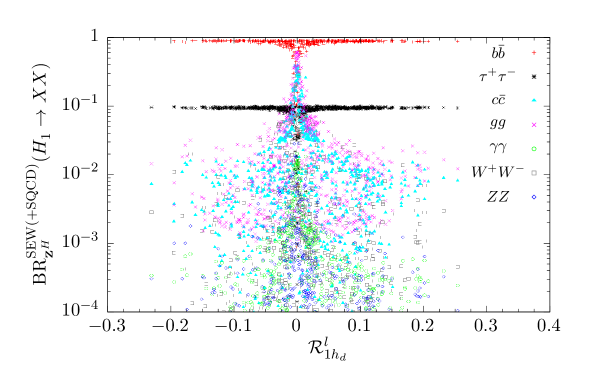
Figure 1: Scan1: Loop-corrected branching ratios of the lightest Higgs boson, which is the singlet-like state, into SM particles versus the element ${\cal R}^{l}_{1h_{d}}$ of the loop-corrected Higgs rotation matrix.

The SM-like Higgs boson is given by the $h_{u}$-like Higgs state, and in our scans we found valid scenarios where this can be the lightest or the second lightest of the CP-even Higgs bosons. We first consider only the parameter points where the lightest CP-even Higgs boson $H_{1}$ is the singlet-like state, i.e. has a large $h_{s}$ component. These are points obtained in the above described scan1. Here and in the following we denote a Higgs boson $H_{i}$ to be dominantly $x$-like ($x=h_{s},h_{u},h_{d},a_{s},a_{d}$) if the corresponding matrix element squared $|{\cal R}^{l}_{ix}|^{2}$ exceeds 80%. When $H_{1}$ is $h_{s}$-like, the question which final state has the largest decay width strongly depends on the amount of admixture of $h_{d}$ and $h_{u}$ components to the singlet-state. In Fig. 1 we show, for all parameter points that pass our constraints, the scatter plot of the $H_{1}$ branching ratios into SM particles against its $h_{d}$ component represented by the element ${\cal R}^{l}_{1h_{d}}$ of the loop-corrected Higgs rotation matrix. The mass of $H_{1}$ lies between 70 and 118 GeV for these points. As can be inferred from the plot, the dominant decays are those into $b\bar{b}$, $c\bar{c}$, $\tau\bar{\tau}$ and $gg$. In most cases the branching ratio into a bottom-quark pair is dominant followed by the decay into $\tau\tau$. However, when the $h_{d}$ component of $H_{1}$ is very small the branching ratios into $gg$ and $c\bar{c}$ become competitive and can even be larger than those for the decay into $b\bar{b}$ with values beyond 60% for the $gg$ final state and of up to 35-39% for $c\bar{c}$ in some of the scenarios. In this case, i.e. for $|{\cal R}^{l}_{1h_{d}}|\raisebox{-3.69899pt}{~{}\shortstack{$<$ \\ [-0.07cm] $\sim$}}~{}0.02$, also the branching ratios into $\gamma\gamma$ and into the off-shell final state $W^{+*}W^{*-}$ increase and can reach up to about 30% in the latter and about 2% in the former case. The branching ratio into the off-shell $Z^{*}Z^{*}$ final state, which also increases then, is about one order of magnitude smaller than the one into $W^{+*}W^{-*}$. But already for $|{\cal R}^{l}_{1h_{d}}|\raisebox{-3.69899pt}{~{}\shortstack{$>$ \\ [-0.07cm] $\sim$}}~{}0.02$ the decay into $b\bar{b}$ takes over again and reaches branching ratio values of up to 90% followed by the branching ratio into $\tau\tau$ with values of up to 10%.

In order to investigate the importance of the higher-order corrections we define for our new implementation the relative correction of the partial width for the decay $H_{i}\to X_{j}X_{k}$ as

$$\delta^{\text{SEW(+SQCD)}}(H_{i}X_{j}X_{k})=\frac{\Gamma^{\text{SEW(+SQCD)}}_{{\bf Z}^{H}}(H_{i}\to X_{j}X_{k})-\Gamma^{\text{tree}}_{{\bf Z}^{H}}(H_{i}\to X_{j}X_{k})}{\Gamma^{\text{tree}}_{{\bf Z}^{H}}(H_{i}\to X_{j}X_{k})}\;,$$ (5.227)

with the higher-order decay widths for the decays $H_{i}\to q\bar{q}$ into quarks given in Eq. (4.138) and the higher-order decay widths for the decays $H_{i}\to l\bar{l}$ into leptons given in Eq. (4.159) and with the tree-level decay width $\Gamma^{\text{tree}}_{{\bf Z}^{H}}$ including only the $\Delta_{b}$ corrections. The tree-level and higher-order decay widths are both evaluated with the new implementation of ${\bf Z}^{H}$. Note that the quantity $\delta$ gives information on the importance of the SEW(+SQCD) corrections in the decay width alone as the factor ${\bf Z}^{H}$ cancels in the ratio. In Fig. 2 we show the scatter plot of the relative change of the branching ratios, $\Delta_{\text{BR}}(H_{1}f\bar{f})$, $f=b,c,\tau$, for all the parameter points passing the constraints, against $\text{BR}_{{\bf Z}^{H}}^{\text{SEW(+SQCD)}}(H_{1}\to f\bar{f})$.

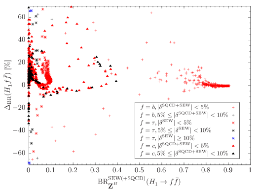
Figure 2: Scan1: Relative difference $\Delta_{\text{BR}}$ (see text, for definition) in percent for the $H_{1}$ decays into $b\bar{b},\tau\bar{\tau},c\bar{c}$. Red: relative corrections $\delta$ (see text, for definition) in percent of the SUSY-EW(+SUSY-QCD) corrections to the decay widths with $|\delta|<5$%; black: $5\leq|\delta|<10$%; blue: $|\delta|\geq 10$%.

The color code in Fig. 2 as well as in Figs. 3–6 denotes the sizes of the relative corrections of the partial decay widths. The points where the absolute value of $\delta^{\text{SEW(+SQCD)}}$ exceeds 10% are marked in blue, those with $\left|\delta^{\text{SEW(+SQCD)}}\right|$ in the [5,10]% range in black and those with relative corrections less than 5% in red. For Figs. 5b and 6b we distinguish two regimes for the larger corrections, in blue where $\left|\delta^{\text{SEW+SQCD}}\right|$ is in the [10,20]% range and in green where $\left|\delta^{\text{SEW+SQCD}}\right|$ is in the [20,40]% range; in Fig. 4b we also add two other categories of points, in cyan where $\left|\delta^{\text{SEW+SQCD}}\right|$ is in the [40,60]% range and in pink where $\left|\delta^{\text{SEW+SQCD}}\right|$ is in the [60,80]% range. Note that for the $\tau$ decays there are no SUSY-QCD corrections. The ballpark of the relative change $\Delta_{\text{BR}}({H_{1}b\bar{b}})$ in the branching ratios between the old and the new implementation ranges below about 30% with vertex corrections $|\delta|$ smaller than 5%. There are some very rare scenarios where $\left|\Delta({H_{1}b\bar{b}})\right|$ exceeds 50% and where at the same time the relative vertex corrections are between 5 and 10%. We investigated these cases and observed that there is an accidental cancellation either in the effective tree-level or in the improved couplings. These parameter points lead to similar results for the $\tau$ final states, i.e. $|\Delta_{\text{BR}}({H_{1}\tau\bar{\tau}})|>50$% and at the same time $|\delta|$ between 5 and 10%. The cancellation results in a suppression of the branching ratio, to less than 4% for the $\tau\bar{\tau}$ final state and 10% at maximum for the $b\bar{b}$ final state. In most of the cases, the large $\Delta_{\text{BR}}({H_{1}f\bar{f}})$ is due to the use of the wave-function renormalization factor ${\bf Z}^{H}$, however. There are also cases with a cancellation between the SUSY-EW/SUSY-QCD corrections and the wave-function renormalization factor ${\bf Z}^{H}$ correction. This results in $\Delta_{\text{BR}}({H_{1}c\bar{c}})$ being less than 1%.

We have performed the same analysis for the heavier Higgs bosons, using the full set of points from our scan2. Figure 3 is the scatter plot of the $\Delta_{\text{BR}}({hf\bar{f}})$, $f=b,\tau,c,t$, against $\text{BR}_{{\bf Z}^{H}}^{\text{SEW(+SQCD)}}(h\to f\bar{f})$ for an SM-like Higgs boson $h$, while Figures 4, 5, and 6 are the scatter plots of $\Delta_{\text{BR}}({H_{i}f\bar{f}})$, $f=b,t$, against $\text{BR}_{{\bf Z}^{H}}^{\text{SEW(+SQCD)}}(H_{i}\to f\bar{f})$ for a heavy $a_{s}$-, $a$- and $h_{d}$-like Higgs boson i.e. $H_{i}=H_{a_{s}}$, $H_{a}$, $H_{h_{d}}$, respectively. As before, the SM-like Higgs boson $h$ is always $h_{u}$-like and decays dominantly into a bottom-quark pair with a branching ratio of about 60%, as expected, followed by the decay into a $\tau$ pair and the decay into a $c$-quark pair. As can be inferred from Fig. 3, the relative changes between the old and the new implementation are much smaller than for the singlet-like lightest Higgs boson and amount only to a few percent. The relative vertex corrections $|\delta|$ are below 10% for the $b$-quark pair final state and below 5% for the decays both into $\tau\bar{\tau}$ and $c\bar{c}$.

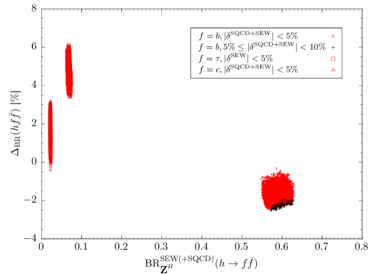
Figure 3: Scan2: Same as Fig. 2 but for the SM-like Higgs boson $h$ that is $h_{u}$-like.

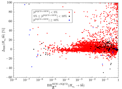
(a)

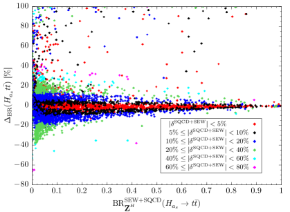
(b)

Figure 4: Scan2: Same as Fig. 2 but for the heavier $a_{s}$-like Higgs boson $H_{a_{s}}$ decaying into $b\bar{b}$ (left) and $t\bar{t}$ (right).

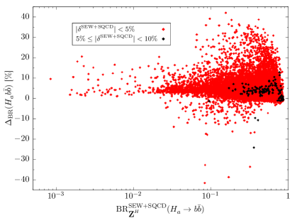
(a)

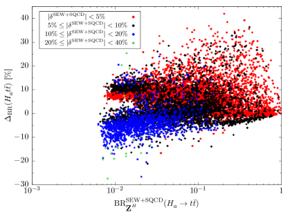
(b)

Figure 5: Scan2: Same as Fig. 2 but for the heavier $a$-like Higgs boson $H_{a}$ decaying into $b\bar{b}$ (left) and $t\bar{t}$ (right).

For the heavy Higgs bosons, the decay into a top quark pair can become kinematically possible. We start by discussing the decay pattern of the heavy singlet state $H_{a_{s}}$, with a mass between 120 GeV and 1.7 TeV, into the $b$-quark and $t$-quark final states, presented in Fig. 4. For the $b\bar{b}$ final states the relative change in the branching ratios due to the new implementation is mostly between -20% and 20%. We also find points where the relative change is close to 100%, in particular for branching ratios close to 100%. Most points exhibit small relative vertex corrections (see, red points in Fig. 4a), so that the large changes of $\Delta_{\text{BR}}(H_{a_{s}}b\bar{b})$ are due to the implementation of ${\bf Z}^{H}$. This is especially the case for large branching ratios close to 100%. There are a few points where the relative vertex corrections lie between 5 and 10% (black) and even above 10% (blue). This happens for the cases where the effective tree-level couplings $H_{a_{s}}f\bar{f}$ are suppressed. The relative change $\Delta_{\text{BR}}$ can still be very small when the effects from the ${\bf Z}^{H}$ factor and the vertex corrections cancel. The decay pattern for the $t\bar{t}$ channel, finally, is displayed in Fig. 4b. The branching ratio takes all values between almost 0 and 100%. The relative changes $\Delta_{\text{BR}}(H_{a_{s}}t\bar{t})$ are mostly between -20% and 20% and close to 0% for large branching ratios above about 60%. We also observe large $\Delta_{\text{BR}}$, in particular for branching ratios close to zero. This is mainly due to very suppressed effective tree-level $H_{a_{s}}t\bar{t}$ couplings corresponding to the regions where the branching ratio $\mathrm{BR}(H_{a_{s}}\to b\bar{b})$ is enhanced. These regions correspond to large values of $\tan\beta$ close to the upper bound in our scan, or to smaller mass values of $H_{a_{s}}$ with not sufficient phase space to decay into an on-shell top-quark pair. In these regions the relative corrections $|\delta|$ are most of the time below 40%, and for cases where $|\delta|<5\%$ the large changes in $\Delta_{\text{BR}}$ are mostly due to the use of the wave-function renormalization factor ${\bf Z}^{H}$. For larger branching ratios the relative corrections $|\delta|$ are mostly below 10% (red and black points). Some rare scenarios display corrections above 40% and up to 80% (in cyan and in pink), again mostly in regions with lower branching ratios.

Similar observations can be made for the other heavier Higgs states $H_{a}$ (with a mass between 539 GeV and 2 TeV) and $H_{h_{d}}$ (with a mass between 548 GeV and 2 TeV), with the notable exception that the relative changes $\Delta_{\text{BR}}({H_{a/h_{d}}}X_{i}X_{j})$ are more reduced and never reach 100%. The relative changes $\Delta_{\mathrm{BR}}(H_{a/h_{d}}b\bar{b})$ are most of the time positive and below 40% as seen in Figs. 5a and 6a. The decays into top-quark pairs can be dominant where the decays into $b\bar{b}$ are suppressed, and the relative changes $\Delta_{\text{BR}}$ between the old and new implementation are close to zero when $\mathrm{BR}(H_{a/h_{d}}\to t\bar{t})\to 100\%$ as seen in Figs. 5b and 6b. For some rare scenarios the relative vertex corrections $|\delta|$ can reach 40%, depicted in green in the figures. Note that $\mathrm{BR}(H_{a/h_{d}}\to b\bar{b})$ can reach 90%, corresponding to regions where the effective tree-level coupling $H_{a/h_{d}}b\bar{b}$ is strongly enhanced due to large values of $\tan\beta$ while at the same time the effective tree-level coupling $H_{a/h_{d}}t\bar{t}$ is strongly suppressed.

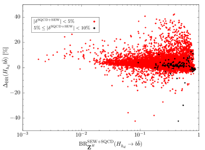
(a)

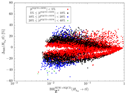
(b)

Figure 6: Scan2: Same as Fig. 2 but for the heavier $h_{d}$-like Higgs boson $H_{h_{d}}$ decaying into $b\bar{b}$ (left) and $t\bar{t}$ (right).

5.2 Decays into a Massive Gauge Boson Pair

In the CP-conserving case, the heavy Higgs boson that can decay into two on-shell massive gauge bosons is $h_{d}$-like. The tree-level coupling of a Higgs boson $H_{i}$ to $VV$ ($V=W,Z$) is proportional to

$${\cal R}_{i,1}{c_{\beta}}+{\cal R}_{i,2}{s_{\beta}}\;.$$ (5.228)

Due to the SM-like (i.e. $h_{u}$-like) Higgs boson coupling with almost SM-strength to the massive gauge bosons the tree-level coupling of the $h_{d}$-like heavy Higgs boson to $VV$ is almost zero because of sum rules. This leads to very suppressed tree-level partial decay widths $\Gamma(H_{h_{d}}\to VV)$.

(a)

(b)

Figure 7: Scan2: Relative difference $\Delta_{\text{BR}}$ in percent for the $h_{d}$-like Higgs boson $H_{h_{d}}$ into a $W$ boson pair (left) and into a $Z$ boson pair (right) as a function of the corresponding loop-corrected branching ratio. Black: relative corrections $\delta^{\text{SEW}}$ in percent of the SUSY-EW corrections to the decay widths with $|\delta^{\text{SEW}}|<20$%; blue: $20\leq|\delta^{\text{SEW}}|<40$%; pink: $40\leq|\delta^{\text{SEW}}|<60$%; green: $60\leq|\delta^{\text{SEW}}|<80$%; cyan: $80\leq|\delta^{\text{SEW}}|<100$%; red: $|\delta^{\text{SEW}}|\geq 100$%.

In order to compare the results obtained in this paper with the old implementation in NMSSMCALC using the tree-level coupling together with the loop-corrected rotation matrix ${\cal R}^{l}$, we show in Fig. 7a the relative change $\Delta_{\text{BR}}(H_{h_{d}}WW)$ of the branching ratio into $WW$ between the old and the new implementation including the NLO-EW vertex corrections as described in Sec. 4.2 and the improvement with the ${\bf Z}^{H}$ factor, as a function of the loop-corrected branching ratio ${\rm BR}_{{\bf Z}^{H}}^{\rm SEW}(H_{h_{d}}\to W^{+}W^{-})$. The plotted points are those of our scan that pass the constraints we have applied. We display in Fig. 7b the same but for the decay into $ZZ$. The color and symbol code denotes the magnitude of the relative NLO electroweak vertex corrections alone, with $\delta$ defined in Eq. (5.227). As can be inferred from the plots both the ${\bf Z}^{H}$ factor and the NLO electroweak corrections can be responsible for the large relative changes in the branching ratios. This is in particular reflected by the black points for which the vertex corrections are below 20% and at the same time the relative changes $\Delta_{\text{BR}}$ can reach up to 100%. In some cases there is a cancellation between the two contributions (the vertex corrections and the ${\bf Z}^{H}$ factor) leading to relatively small relative changes in the branching ratios. These cases are the pentagon-marked full (red) points in Fig. 7a for the decay $H_{h_{d}}\to W^{+}W^{-}$, which are mostly located in regions where $|\Delta_{\text{BR}}(H_{h_{d}}WW)|\raisebox{-3.69899pt}{~{}\shortstack{$<$ \\ [-0.07cm] $\sim$}}~{}25\%$ while the relative vertex correction $|\delta|$ is at least 100%. In the case of the decay into a $Z$ boson pair, however, the bulk of these pentagon-marked full (red) points, indicating again a relative vertex correction $|\delta|$ of at least 100%, induces large relative changes of $\Delta_{\text{BR}}(H_{h_{d}}ZZ)$ close to 100%. These points correspond to a region which is discussed in more detail in the next paragraph.

We also note that there are two regions concentrating many points for the decay into a $Z$ boson pair, the region for which $\Delta_{\text{BR}}(H_{h_{d}}ZZ)\simeq 0$% and the one for which $\Delta_{\text{BR}}(H_{h_{d}}ZZ)\simeq 100$%. This is in contrast to the decay into a $W$ boson pair which is mostly centered around $\Delta_{\text{BR}}(H_{h_{d}}WW)\simeq 0$% for vertex corrections $|\delta|<80$% and much more scattered for the points where $80<|\delta|<100$%, displayed with cyan-pentagon-marked points (for $|\delta|\geq 100$% the above described cancellation takes place in the decay $H_{h_{d}}\to W^{+}W^{-}$). This presence of the second region in the $Z$ boson final state, for which $\Delta_{\text{BR}}$ is close to 100% can be explained by the occurrence of many parameter points having a very suppressed tree-level coupling $H_{h_{d}}ZZ$. They also correspond to regions where the loop-corrected partial decay width $\Gamma(H_{h_{d}}\to ZZ)$ is higher, up to 1 GeV, while the decay width is at most 5 MeV for the region centered around $\Delta_{\text{BR}}(H_{h_{d}}ZZ)=0$. Note, that while the tree-level couplings $H_{h_{d}}ZZ$ and $H_{h_{d}}WW$ are the same, the loop-corrected decay widths differ by the fact that the decay into $WW$ bosons receives real corrections and that in the one-loop squared contributions to the decay width $H_{h_{d}}\to W^{+}W^{-}$ we only include the (s)fermion contributions in contrast to the decay $H_{h_{d}}\to ZZ$.

5.3 Decays into a $Z$ Boson and a Higgs Boson

In the searches for heavy pseudoscalars, this decay can be an important search channel [82, 83]. We are interested here in how large the branching ratio can be and how important are the newly included higher-order corrections, in the case for which on-shell decays are possible. With the obtained valid set of parameter points, we present in Fig. 8a scatter plots of the relative changes of the branching ratios between the old and new implementation for the decay of a heavy pseudoscalar-like Higgs boson $H_{a}$ into $ZH_{1}$ and in Fig. 8b for the decay into $ZH_{2}$, against the respective loop-corrected branching ratios. The color and marker codes denote the relative sizes of the one-loop vertex corrections within specific ranges, identical to the ranges used in the previous sub-section for the decays into gauge boson pairs. The mass values of the individual involved CP-even Higgs bosons in the final state range in $123~{}\text{GeV}\leq m_{H_{1}}\leq 127~{}\text{GeV}$ and $463~{}\text{GeV}\leq m_{H_{2}}\leq 1.73~{}\text{TeV}$, while the mass of the decaying Higgs boson ranges in $539~{}\text{GeV}\leq m_{H_{a}}\leq 2.0~{}\text{TeV}$ for the on-shell decay into $ZH_{1}$ pairs and in $713~{}\text{GeV}\leq m_{H_{a}}\leq 2.0~{}\text{TeV}$ for the on-shell decay into $ZH_{2}$ pairs. As can already be inferred from the mass ranges, the $H_{1}$ state is the SM-like Higgs boson $h$, while the $H_{2}$ state is the singlet-like scalar Higgs boson $H_{h_{s}}$.

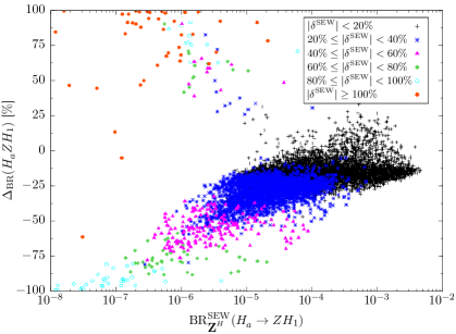
(a)

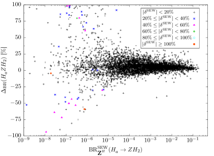
(b)

Figure 8: Scan2: Relative difference $\Delta_{\text{BR}}$ in percent for the $H_{a}$-like Higgs boson decay into $ZH_{1}$ (left) and into $ZH_{2}$ (right) as a function of the corresponding loop-corrected branching ratio. Black: relative corrections $\delta^{\text{SEW}}$ in percent of the SUSY-EW corrections to the decay widths with $|\delta^{\text{SEW}}|<20$%; blue: $20\leq|\delta^{\text{SEW}}|<40$%; pink: $40\leq|\delta^{\text{SEW}}|<60$%; green: $60\leq|\delta^{\text{SEW}}|<80$%; cyan: $80\leq|\delta^{\text{SEW}}|<100$%; red: $|\delta^{\text{SEW}}|\geq 100$%.

We observe that the branching ratios into the $ZH_{1}$ final state remain very small, below 0.4%, while those of the decay into $ZH_{2}$ can reach 11%. This is due to the nature of the $H_{1}$ Higgs boson that is SM-like, with very suppressed tree-level $H_{1}H_{a}Z$ couplings. The relative changes $\Delta_{\text{BR}}$ of the branching ratio for the decay $H_{a}\to ZH_{1}$ are mostly between 0 and -75% corresponding to relative vertex corrections $|\delta^{\text{SEW}}|$ being at most 60% (black, blue, and pink points), while a few points corresponding to higher vertex corrections up to more than 100% (green, cyan, and red points) can reach $\Delta_{\text{BR}}=\pm 100$%. These extreme points correspond to very small values for the branching ratios themselves which explains in turn the very large relative corrections $|\delta|$ that we observe. Note that in these decays we take into account the one-loop squared term as described in Eq. (4.191) which makes up for the main contribution to the very large relative corrections. As for the decay $H_{a}\to ZH_{2}$ the relative correction $\Delta_{\text{BR}}$ is most of the time between 0 and $\pm 25$%, corresponding to points where the relative vertex corrections $|\delta|$ are below 20%. A few points display larger $\Delta_{\text{BR}}$ values, and also larger relative vertex corrections $|\delta|$ that can reach 100% and even beyond, again for points that display very small branching ratios, below about $10^{-4}\,\%$. Note that there are points for which the correction $|\Delta_{\text{BR}}|$ is rather limited, below 25%, while the relative vertex correction can reach 40% (for one scenario even more than 100%). This can be explained by a sign compensation between the ${\bf Z}^{H}$ factor and the vertex correction.

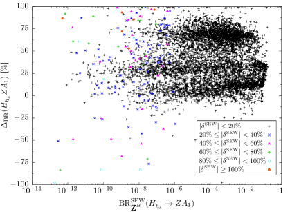
(a)

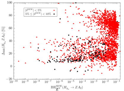
(b)

Figure 9: Scan2: Same as in Fig. 8 but for a heavy singlet-like Higgs boson $H_{h_{s}}$ decaying into $ZA_{1}$ and $ZA_{2}$ pairs. In the right plot, however, red: $|\delta^{\text{SEW}}|<5\%$; black: $5\leq|\delta^{\text{SEW}}|<10\%$.

The corresponding results for the heavy singlet-like Higgs boson $H_{h_{s}}$ decaying into $ZA_{1}$ and $ZA_{2}$ are shown in Figs. 9a and Figs. 9b, respectively. We see that the maximum achieved branching ratios for the decay $H_{h_{s}}\to ZA_{1}$ are below 20% and for a large number of parameter points are tiny. In the case of the decay $H_{h_{s}}\to ZA_{2}$ the branching ratio can reach around 15%. In most of the cases $A_{1}$ is singlet-like, corresponding to points where the branching ratio is small (below 10%), while $A_{2}$ is doublet-like. The mass values of the individual involved Higgs bosons in the final state range in $120~{}\text{GeV}\leq m_{A_{1}}\leq 1.50~{}\text{TeV}$ and $562~{}\text{GeV}\leq m_{A_{2}}\leq 1.63~{}\text{TeV}$, while the mass of the decaying Higgs boson ranges in $464~{}\text{GeV}\leq m_{H_{h_{s}}}\leq 1.75~{}\text{TeV}$ for the on-shell decay into $ZA_{1}$ pairs and in $696~{}\text{GeV}\leq m_{H_{h_{s}}}\leq 1.75~{}\text{TeV}$ for the on-shell decay into $ZH_{2}$ pairs. The cases with larger branching ratios for the decay $H_{h_{s}}\to ZA_{1}$ (larger than 10%) correspond mostly to the few $A_{1}$ pseudoscalar Higgs bosons with doublet-like admixture and mass values above $400$ GeV.

The relative changes $\Delta_{\mathrm{BR}}$ in the branching ratios are mostly positive, and can reach values of 100%. For some very rare scenarios we get $\Delta_{\mathrm{BR}}(H_{h_{s}}ZA_{1})$ close to -100%, while $\Delta_{\mathrm{BR}}(H_{h_{s}}ZA_{2})$ is not below -15%. The relative vertex corrections are moderate for the decay $H_{h_{s}}\to ZA_{1}$, mostly $|\delta|\leq 20$% (black points). This means that the large changes in $\Delta_{\mathrm{BR}}(H_{h_{s}}ZA_{1})$ are mostly due to the ${\bf Z}^{H}$ factor. For very small branching fractions below $10^{-4}\%$ larger vertex corrections are possible, mainly because the denominator in the definition of $\delta$ is very small in these regions and can lead to sharp changes in $\delta$. Note that the bulk of the changes between the old and the new implementation in these cases stems from the vertex corrections. In the case of the decay $H_{h_{s}}\to ZA_{2}$ the relative vertex corrections are mostly small, with values $|\delta|<5$% (red triangle-marked points). For large relative changes $\Delta_{\text{BR}}(H_{h_{s}}ZA_{2})$ the ${\bf Z}^{H}$ factor is responsible then.

5.4 Decays into Charginos and Neutralinos

We start by investigating the loop corrections to the masses of the charginos and neutralinos using the three renormalization schemes OS1, OS2 and $\overline{\text{DR}}$, imposed on the two gaugino masses $M_{1}$ and $M_{2}$, as defined in Section 3.1.2. According to the SLHA format that we apply in our code, $M_{1},M_{2}$ are $\overline{\text{DR}}$ parameters given at the scale $M_{\text{SUSY}}=\sqrt{m_{\tilde{Q}_{3}}m_{\tilde{t}_{R}}}$. When we use the OS schemes we have to translate the $\overline{\text{DR}}$ input parameters to the OS values by applying the approximate transformation formulae

$$M_{1}^{\text{OSi}} = M^{\overline{\text{DR}}}_{1}-\delta M_{1}^{\text{finOSi}}$$

$$M_{2}^{\text{OSi}} = M^{\overline{\text{DR}}}_{2}-\delta M_{2}^{\text{finOSi}}\;,$$ (5.229)

where $\delta M_{1/2}^{\text{finOSi}}$ are the finite parts of the $M_{1/2}$ counterterms computed in the OSi ($i=1,2$) renormalization scheme. Since the finite parts $\delta M_{1/2}^{\text{finOSi}}$ should be computed with OS input parameters we have used an iterative method to obtain these. For all parameter points in our scan, the size of the loop corrections to the neutralino and charginos masses, quantified by $\Delta M^{\tilde{\chi}}_{i}=M_{\tilde{\chi}_{i}}^{\text{loop}}-m_{\tilde{\chi}_{i}}^{\text{tree}}$, with $i=1,...,5$ for the neutralinos and $i=1,2$ for the charginos, never exceeds 46 GeV.

We exemplary present here a particular point, called scenario1, with the soft SUSY breaking masses and trilinear couplings given by

$$m_{\tilde{t}_{R}}=1384\,~{}\text{GeV}\,,\;m_{\tilde{Q}_{3}}=1743\,~{}\text{GeV}\,,\;m_{\tilde{b}_{R}}=m_{\tilde{L}_{3}}=m_{\tilde{\tau}_{R}}=3000\,~{}\text{GeV}\,,$$

$$|A_{u,c,t}|=3594\,~{}\text{GeV}\,,\;|A_{d,s,b}|=2000\,~{}\text{GeV}\,,\;|A_{e,\mu,\tau}|=2000\,~{}\text{GeV}\,,\;$$ (5.230)

$$|M_{1}|=560\,~{}\text{GeV},\;|M_{2}|=684\,~{}\text{GeV}\,,\;|M_{3}|=2494\,~{}\text{GeV}\,,$$

$$\varphi_{A_{e,\mu,\tau}}=\varphi_{A_{d,s,b}}=0\,,\;\varphi_{A_{u,c,t}}=\varphi_{M_{1}}=\varphi_{M_{2}}=\varphi_{M_{3}}=0\;,$$

and the remaining input parameters set to

$$|\lambda|=0.307\;,\quad|\kappa|=0.517\;,\quad\text{Re}\,A_{\kappa}=361\,~{}\text{GeV}\;,\quad|\mu_{\text{eff}}|=272\,~{}\text{GeV}\;,$$

$$\varphi_{\lambda}=\varphi_{\kappa}=\varphi_{u}=0\;,\quad\varphi_{\mu_{\text{eff}}}=\pi\;,\quad\tan\beta=9.38\;,\quad M_{H^{\pm}}=1393\,~{}\text{GeV}\;.$$ (5.231)

The Higgs boson masses and their main composition in terms of singlet/doublet and scalar/pseudoscalar components at two-loop order ${\cal O}(\alpha_{t}\alpha_{s}+\alpha_{t}^{2})$ for $\overline{\text{DR}}$ renormalization in the top/stop sector computed by NMSSMCALC, are summarized in Table 2.

$\overline{\text{DR}}$	${H_{1}}$	${H_{2}}$	${H_{3}}$	${H_{4}}$	${H_{5}}$
two-loop ${\cal O}(\alpha_{t}\alpha_{s}+\alpha_{t}^{2})$	125.14	698.05	813.53	1391.6	1392.56
main component	$h_{u}$	$a_{s}$	$h_{s}$	$a$	$h_{d}$

Table 2: Scenario1: Masses and main components of the neutral Higgs bosons at two-loop order ${\cal O}(\alpha_{t}\alpha_{s}+\alpha_{t}^{2})$, using $\overline{\text{DR}}$ renormalization in the top/stop sector.

For scenario1, we present in Table 3 the tree-level and loop-corrected masses of the neutralinos and charginos in the three different renormalization schemes and for the Denner description. As expected the wino-like neutralino and the wino-like chargino which couple to the electroweak gauge bosons, get significant loop corrections in the $\overline{\text{DR}}$ scheme. The one-loop corrected masses themselves, however, barely differ in the three renormalization schemes so that the remaining theoretical error due to missing higher-order corrections is very small.

		${M_{\tilde{\chi}_{1}^{0}}}$	${M_{\tilde{\chi}^{0}_{2}}}$	${M_{\tilde{\chi}_{3}^{0}}}$	${M_{\tilde{\chi}_{4}^{0}}}$	${M_{\tilde{\chi}_{5}^{0}}}$	${M_{\tilde{\chi}_{1}^{+}}}$	${M_{\tilde{\chi}_{2}^{+}}}$
OS1	tree-level	265.97	276.05	565.2	730.92	920.76	270.72	730.83
	one-loop	273.22	282.48	565.2	730.78	914.39	278.02	730.83
OS2	tree-level	265.97	276.05	565.2	730.78	920.76	270.72	730.69
	one-loop	273.22	282.48	565.2	730.78	914.39	278.02	730.83
$\overline{\text{DR}}$	tree-level	265.5	276.2	563.47	694.32	920.76	270.38	694.18
	one-loop	273.21	282.44	565.21	730.01	914.39	278.01	729.86
	main component	$\tilde{H}_{d}^{0}$	$\tilde{H}_{u}^{0}$	$\tilde{B}$	$\tilde{W}_{3}$	$\tilde{S}$	$\tilde{H}^{+}$	$\tilde{W}^{+}$

Table 3: Scenario1: Masses and main components of the neutralinos and charginos at tree and one-loop level in the three renormalization schemes OS1, OS2 and $\overline{\text{DR}}$.

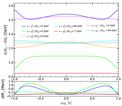
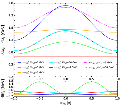
Figure 10: Scenario1: Upper: loop corrections to the electroweakino masses, $\Delta M_{x}$ (see text, for the definition), $x=\tilde{\chi}_{i}^{0},\tilde{\chi}_{j}^{\pm}$ ($i=1,...,5$, $j=1,2$), as a function of $\varphi_{M_{1}}$ (left) and $\varphi_{M_{2}}$ (right) in the $\overline{\text{DR}}$ scheme using the Denner description. The subtraction values $\delta M_{x}$ are specified in the legends. Lower: differences $\text{diff}_{x}$ (see text, for the definition) between the loop-corrected masses using the Denner and the EMT descriptions.

We vary the phases of the gaugino mass parameters $M_{1}$ and $M_{2}$, $\varphi_{M_{1}}$ and $\varphi_{M_{2}}$, in order to study their effect on the loop-corrected neutralino and chargino masses. Note that these complex phases have negligible impact on the Higgs sector [15, 17]. We use the $\overline{\text{DR}}$ scheme for this analysis and show in the upper plots of Fig. 10 the loop corrections to the electroweakino masses,

$$\Delta M_{x}=M_{x}^{\text{loop}}-m_{x}^{\text{tree}}\;,\qquad x=\tilde{\chi}_{i}^{0},\tilde{\chi}_{j}^{\pm}\;(i=1,...,5,j=1,2)\;,$$ (5.232)

as function of $\varphi_{M_{1}}$ (left) and $\varphi_{M_{2}}$ (right). We apply a subtraction $\delta M_{x}$ to the mass corrections $\Delta M_{x}$ of the different electroweakinos that allows us to show all corrections, which can be very different in size, in one plot. In the lower plots of Fig. 10 we show the differences

$$\text{diff}_{x}=M_{x}^{\text{loop,\;D}}-M_{x}^{\text{loop,\;EMT}}\;,$$ (5.233)

with $x$ denoting any electroweakino, between the loop corrected electroweakino masses computed using the Denner and the EMT descriptions presented in Section 3.1.2. As can be inferred from the upper plots, the wino-like neutralino $\tilde{\chi}_{4}^{0}$ (cyan line) and wino-like chargino $\tilde{\chi}_{2}^{+}$ (black line) receive the largest loop corrections of about 35 GeV in absolute values. The corrections to the Higgsino-like neutralinos $\tilde{\chi}_{1}^{0}$ (blue line) and $\tilde{\chi}_{2}^{0}$ (green line), the singlino-like neutralino $\tilde{\chi}_{0}^{5}$ (red line) and the Higgsino-like chargino $\tilde{\chi}_{1}^{+}$ (pink line) range around 6-8 GeV. The correction to the bino-like neutralino $\tilde{\chi}_{3}^{0}$ (orange line) is somewhat smaller with values around 1.5-1.8 GeV. A small difference between the Denner and the EMT descriptions of about 1-2 MeV is observed for the Higgsino-like neutralinos, cf. lower plots. We do not see any difference, however, for the chargino masses. This is because we have used the approximation in Eq. (3.122) for the loop-corrected chargino masses. There is a compensation between $\text{Re}\,\Sigma^{\tilde{\chi}^{+},Ls}_{ii}(m_{\tilde{\chi}_{i}^{\pm}}^{2})$ and $\text{Re}\,\Sigma^{\tilde{\chi}^{+},Rs}_{ii}(m_{\tilde{\chi}_{i}^{\pm}}^{2})$ that kills the effect of the imaginary part of the loop integral function.

		$\Gamma^{l}[~{}\text{MeV}]$	$\delta[\%]$	BRl [$\%$]		$\Gamma^{l}[~{}\text{MeV}]$	$\delta[\%]$	BRl [$\%$]
$H_{2}\to\tilde{\chi}_{1}^{0}\tilde{\chi}_{1}^{0}$	OS1	405.67	0.08	25.14	$H_{2}\to\tilde{\chi}_{1}^{0}\tilde{\chi}_{2}^{0}$	0.43	-0.08	0.03
	$\overline{\text{DR}}$	407.74	8.4	25.15		0.4	-16.34	0.02
$H_{2}\to\tilde{\chi}_{2}^{0}\tilde{\chi}_{2}^{0}$	OS1	404.44	0.07	25.06	$H_{2}\to\tilde{\chi}_{1}^{+}\tilde{\chi}_{1}^{-}$	802.3	0.08	49.72
	$\overline{\text{DR}}$	404.84	7.23	24.98		807.18	9.03	49.8
$H_{3}\to\tilde{\chi}_{1}^{0}\tilde{\chi}_{1}^{0}$	OS1	321.53	0.08	22.01	$H_{3}\to\tilde{\chi}_{1}^{0}\tilde{\chi}_{2}^{0}$	0.78	-0.11	0.05
	$\overline{\text{DR}}$	322.45	8.13	22.04		0.73	-16.24	0.05
$H_{3}\to\tilde{\chi}_{2}^{0}\tilde{\chi}_{2}^{0}$	OS1	308.94	0.07	21.15	$H_{3}\to\tilde{\chi}_{1}^{+}\tilde{\chi}_{1}^{-}$	633.52	0.08	43.38
	$\overline{\text{DR}}$	309.0	7.08	21.12		635.37	8.79	43.42
$H_{4}\to\tilde{\chi}_{1}^{0}\tilde{\chi}_{1}^{0}$	OS1	102.86	0.02	0.8	$H_{5}\to\tilde{\chi}_{1}^{0}\tilde{\chi}_{1}^{0}$	151.31	-0.01	1.18
	$\overline{\text{DR}}$	89.4	-11.31	0.69		132.77	-13.56	1.04
$H_{4}\to\tilde{\chi}_{1}^{0}\tilde{\chi}_{2}^{0}$	OS1	17.87	0.08	0.14	$H_{5}\to\tilde{\chi}_{1}^{0}\tilde{\chi}_{2}^{0}$	9.29	0.24	0.07
	$\overline{\text{DR}}$	14.59	-11.68	0.11		7.65	1.94	0.06
$H_{4}\to\tilde{\chi}_{1}^{0}\tilde{\chi}_{3}^{0}$	OS1	395.9	-5.5	4.59	$H_{5}\to\tilde{\chi}_{1}^{0}\tilde{\chi}_{3}^{0}$	423.04	0.02	3.3
	$\overline{\text{DR}}$	451.86	6.59	3.5		448.9	7.83	3.5
$H_{4}\to\tilde{\chi}_{1}^{0}\tilde{\chi}_{4}^{0}$	OS1	1448.21	-0.03	11.22	$H_{5}\to\tilde{\chi}_{1}^{0}\tilde{\chi}_{4}^{0}$	1161.18	-0.02	9.05
	$\overline{\text{DR}}$	1438.6	-3.68	11.15		1157.98	-2.81	9.03
$H_{4}\to\tilde{\chi}_{1}^{0}\tilde{\chi}_{5}^{0}$	OS1	194.66	-0.02	1.51	$H_{5}\to\tilde{\chi}_{1}^{0}\tilde{\chi}_{5}^{0}$	338.35	-0.02	2.64
	$\overline{\text{DR}}$	195.02	-1.63	1.51		341.12	-1.58	2.66
$H_{4}\to\tilde{\chi}_{2}^{0}\tilde{\chi}_{2}^{0}$	OS1	27.86	-0.13	0.22	$H_{5}\to\tilde{\chi}_{2}^{0}\tilde{\chi}_{2}^{0}$	34.6	-0.1	0.27
	$\overline{\text{DR}}$	25.54	-20.08	0.2		32.72	-15.35	0.26
$H_{4}\to\tilde{\chi}_{2}^{0}\tilde{\chi}_{3}^{0}$	OS1	425.3	0.02	3.29	$H_{5}\to\tilde{\chi}_{2}^{0}\tilde{\chi}_{3}^{0}$	413.74	0.01	3.22
	$\overline{\text{DR}}$	450.13	7.77	3.49		438.11	6.48	3.42
$H_{4}\to\tilde{\chi}_{2}^{0}\tilde{\chi}_{4}^{0}$	OS1	1125.46	-0.02	8.72	$H_{5}\to\tilde{\chi}_{2}^{0}\tilde{\chi}_{4}^{0}$	1379.31	-0.03	10.75
	$\overline{\text{DR}}$	1116.5	-3.34	8.66		1366.13	-3.91	10.66
$H_{4}\to\tilde{\chi}_{2}^{0}\tilde{\chi}_{5}^{0}$	OS1	382.4	-0.02	2.96	$H_{5}\to\tilde{\chi}_{2}^{0}\tilde{\chi}_{5}^{0}$	180.21	-0.02	1.4
	$\overline{\text{DR}}$	381.89	-2.35	2.96		180.34	-1.86	1.41
$H_{4}\to\tilde{\chi}_{3}^{0}\tilde{\chi}_{3}^{0}$	OS1	1.2	0.19	0.01	$H_{5}\to\tilde{\chi}_{3}^{0}\tilde{\chi}_{3}^{0}$	1.19	0.18	0.01
	$\overline{\text{DR}}$	1.29	28.87	0.01		1.29	27.81	0.01
$H_{4}\to\tilde{\chi}_{3}^{0}\tilde{\chi}_{4}^{0}$	OS1	3.18	0.05	0.02	$H_{5}\to\tilde{\chi}_{3}^{0}\tilde{\chi}_{4}^{0}$	1.48	0.06	0.01
	$\overline{\text{DR}}$	2.95	-2.79	0.02		1.43	0.89	0.01
$H_{4}\to\tilde{\chi}_{1}^{+}\tilde{\chi}_{1}^{-}$	OS1	393.59	-0.01	3.05	$H_{5}\to\tilde{\chi}_{1}^{+}\tilde{\chi}_{1}^{-}$	257.68	-0.03	2.01
	$\overline{\text{DR}}$	343.95	-13.61	2.67		215.16	-19.09	1.68
$H_{4}\to\tilde{\chi}_{1}^{+}\tilde{\chi}_{2}^{-}$	OS1	2440.51	-0.01	18.91	$H_{5}\to\tilde{\chi}_{1}^{+}\tilde{\chi}_{2}^{-}$	2482.01	-0.01	19.34
	$\overline{\text{DR}}$	2461.41	-0.61	19.0		2498.8	-0.9	19.49
$H_{4}\to\tilde{\chi}_{2}^{+}\tilde{\chi}_{1}^{-}$	OS1	2440.51	-0.01	18.91	$H_{5}\to\tilde{\chi}_{2}^{+}\tilde{\chi}_{1}^{-}$	2482.01	-0.01	19.34
	$\overline{\text{DR}}$	2461.41	-0.61	19.0		2498.8	-0.9	19.49

Table 4: Scenario 1: Loop-corrected decay widths $\Gamma^{l}$, relative loop corrections $\delta$ and loop-corrected branching ratios BR^l of all kinematically allowed decays into chargino and neutralino pairs of heavy Higgs bosons in the OS1 and $\overline{\text{DR}}$ renormalization schemes. The results in the OS2 scheme are nearly the same as in OS1 scheme.

In order to study the loop corrections on the decay widths, we computed the tree-level and loop-corrected decay widths, defined in Section 4.4, for the three different renormalization schemes OS1, OS2 and $\overline{\text{DR}}$ for the scenario1. Note that we use the loop-corrected masses for external Higgs bosons, charginos and neutralinos not only in the loop-corrected decay widths but also in the tree-level ones. For illustration, we present in Table 4 for the decays of all Higgs bosons in all possible electroweakino final states the loop-corrected decay widths $\Gamma^{l}\equiv\Gamma_{{\bf Z}^{H}}^{\text{SEW}}(H_{i}\to\tilde{\chi}_{j}\tilde{\chi}_{k})$, the relative corrections $\delta(H_{i}\tilde{\chi}_{j}\tilde{\chi}_{k})$ as defined in Eq. (5.227), and the loop-corrected branching ratios $\mbox{BR}^{l}\equiv\mbox{BR}_{{\bf Z}^{H}}^{\text{SEW}}(H_{i}\to\tilde{\chi}_{j}\tilde{\chi}_{k})$ using scenario1, for the OS1 and $\overline{\text{DR}}$ renormalization schemes. We found that $\Gamma^{l}$ is almost identical in the two OS schemes. The relative size of the loop corrections is below 10% in the OS scheme. The relative corrections in the $\overline{\text{DR}}$ scheme are always larger than in the OS schemes. For some channels with small decay widths, we see significant corrections in the $\overline{\text{DR}}$ scheme. For example in the decay channel $H_{4}\to\tilde{\chi}_{2}^{0}\tilde{\chi}_{2}^{0}$, the relative loop correction is $-0.13\%$ in the OS scheme while it is $-20\%$ in the $\overline{\text{DR}}$ scheme. Based on our investigation, we conclude that it is better to use the OS scheme in the decays of the neutral Higgs bosons into electroweakinos. The largest uncertainty due to missing higher-order corrections that we estimate from the variation of the renormalization schemes is found to be 17% in the decay $H_{5}\to\tilde{\chi}_{1}^{0}\tilde{\chi}_{2}^{0}$. We also studied the difference between the Denner and EMT descriptions and did not observe any significant difference. Defining the difference as $(\Gamma^{\text{D}}_{x}-\Gamma^{\text{EMT}}_{x})/\Gamma^{\text{D}}_{x}$ with $\Gamma_{x}$ being the loop-corrected decay width for some Higgs decay into an electroweakino final state, we see that the differences are of per mille level for all investigated decays.

5.5 Decays into a Squark Pair

We start by discussing the top and bottom squark masses in the OS and $\overline{\text{DR}}$ renormalization schemes defined in Section 3.1.3. We follow the SLHA convention where the input parameters $m_{\tilde{Q}_{3}},m_{\tilde{t}_{R}},m_{\tilde{b}_{R}},A_{t},A_{b}$ are $\overline{\text{DR}}$ parameters at the scale $M_{\text{SUSY}}$. When we apply the OS scheme, these parameters must be translated into OS parameters by applying the approximate transformation formula ($i=1,2$)

$$X^{\text{OSi}}=X^{\overline{\text{DR}}}-\delta X^{\text{finOSi}}\;,$$ (5.234)

with $X=m_{\tilde{Q}_{3}},m_{\tilde{t}_{R}},m_{\tilde{b}_{R}},A_{t},A_{b}$ and the finite part of their OS counterterms denoted as $\delta X^{\text{finOSi}}$. We have used an iterative method to obtain a stable value of $\delta X^{\text{finOSi}}$. Note that we include both the NLO QCD and the full NLO EW contribution in the conversion Eq. (5.234). Using these OS parameters together with the OS top mass in the tree-level mass matrices, we obtain the top and bottom squark masses. When we apply the $\overline{\text{DR}}$ renormalization scheme, the top pole mass has to be translated to the $\overline{\text{DR}}$ top mass for which we follow the description in appendix C of Ref. [17]. The $\overline{\text{DR}}$ top and bottom masses together with the $\overline{\text{DR}}$ parameters $m_{\tilde{Q}_{3}},m_{\tilde{t}_{R}},m_{\tilde{b}_{R}},A_{t},A_{b}$ are then used in the tree-level mass matrices to get the tree-level rotation matrices. They are subsequently used in the computation of the renormalized self-energies of the top and bottom squarks to obtain the loop-corrected squark masses as described in Section 3.4. In principle, we would expect that the loop-corrected masses computed in the $\overline{\text{DR}}$ scheme are closer to the OS masses in the OS description if one includes more higher order corrections. We consider here a parameter point (scenario2) given by the following soft SUSY breaking masses and trilinear couplings

$$m_{\tilde{u}_{R},\tilde{c}_{R}}=m_{\tilde{d}_{R},\tilde{s}_{R}}=m_{\tilde{Q}_{1,2}}=m_{\tilde{L}_{1,2}}=m_{\tilde{e}_{R},\tilde{\mu}_{R}}=3\;\mbox{TeV}\,,\;m_{\tilde{t}_{R}}=623\,~{}\text{GeV}\,,\;$$

$$m_{\tilde{Q}_{3}}=1180\,~{}\text{GeV}\,,\;m_{\tilde{b}_{R}}=m_{\tilde{L}_{3}}=m_{\tilde{\tau}_{R}}=33\;\mbox{TeV}\,,$$

$$|A_{u,c,t}|=1760\,~{}\text{GeV}\,,\;|A_{d,s,b}|=2000\,~{}\text{GeV}\,,\;|A_{e,\mu,\tau}|=2000\,~{}\text{GeV}\,,\;$$ (5.235)

$$|M_{1}|=1000\,~{}\text{GeV},\;|M_{2}|=1251\,~{}\text{GeV}\,,\;|M_{3}|=2364\,~{}\text{GeV}\;,$$

with the CP phases given by

$$\varphi_{A_{u,c,t}}=\varphi_{A_{d,s,b}}=\varphi_{A_{e,\mu,\tau}}=\varphi_{M_{1}}=\varphi_{M_{2}}=\varphi_{M_{3}}=0\;.$$ (5.236)

The remaining input parameters have been set to

$$\lambda=0.106\;,\quad\kappa=-0.238\;,\quad\mbox{Re}(A_{\kappa})=-647\,~{}\text{GeV}\;,\quad\mu_{\text{eff}}=-603\,~{}\text{GeV}\;,$$

$$\varphi_{u}=0\;,\quad\tan\beta=17.5\;,\quad M_{H^{\pm}}=1867\,~{}\text{GeV}\;.$$ (5.237)

With the given $\overline{\text{DR}}$ parameters of the squark sector, we obtain their corresponding OS parameters

$$m_{\tilde{Q}_{3}}=1120\,~{}\text{GeV}\;,\quad m_{\tilde{t}_{R}}=402\,~{}\text{GeV}\;,\quad m_{\tilde{b}_{R}}=2997\,~{}\text{GeV}\;,$$

$$\quad A_{t}=1720\,~{}\text{GeV}\;,\quad A_{b}=-581\,~{}\text{GeV}\>.$$ (5.238)

The tree-level and loop-corrected masses of the stops and sbottoms in the OS and $\overline{\text{DR}}$ scheme are shown in Table 5. We see that for the $\overline{\text{DR}}$ scheme there are large changes between the tree-level and one-loop masses, in particular for the lightest stop $\tilde{t}_{1}$. The loop-corrected masses, however, are then closer to each other in both schemes, as expected. The maximum difference if found for the light sbottom $\tilde{b}_{1}$ mass, where the OS and $\overline{\text{DR}}$ results differ by 27 GeV at one-loop order (compared to 59 GeV at tree level). The two-loop corrected neutral Higgs boson masses at ${\cal O}(\alpha_{t}\alpha_{s}+\alpha_{t}^{2})$ together with their respective main component are displayed in Table 6. The SM-like Higgs boson mass is around 124 GeV while the remaining Higgs spectrum is quite heavy with masses above 1.6 TeV.

		$m_{\tilde{t}_{1}}\,[\mbox{GeV}]$	$m_{\tilde{t}_{2}}\,[\mbox{GeV}]$	$m_{\tilde{b}_{1}}\,[\mbox{GeV}]$	$m_{\tilde{b}_{2}}\,[\mbox{GeV}]$
OS	tree	334	1166	1122	2297
	1loop	334	1166	1125	2297
$\overline{\text{DR}}$	tree	585	1216	1181	3000
	1loop	341	1152	1152	2294

Table 5: Scenario2: The tree-level and one-loop corrected stop and sbottom masses in the $\overline{\text{DR}}$ and OS schemes.

	${H_{1}}$	${H_{2}}$	${H_{3}}$	${H_{4}}$	${H_{5}}$
two-loop ${\cal O}(\alpha_{t}\alpha_{s}+\alpha_{t}^{2})$	123.63	1621.65	1865.39	1895.83	2538.29
main component	$h_{u}$	$a_{s}$	$h_{d}$	$a$	$h_{s}$

Table 6: Scenario2: Mass values in GeV and main components of the neutral Higgs bosons at two-loop order ${\cal O}(\alpha_{t}\alpha_{s}+\alpha_{t}^{2})$ obtained by using the $\overline{\text{DR}}$ renormalization in the top/stop sector.

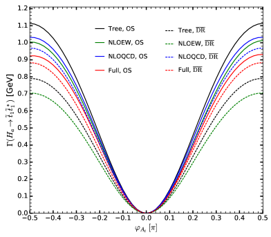
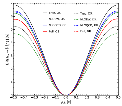
Figure 11: Scenario2: Tree-level (black), NLO EW (green), NLO QCD (blue) and full (red) partial width (left) and branching ratio (right) of the decay $H_{4}\to\tilde{t}_{1}\tilde{t}_{1}^{*}$ ($H_{4}$ is $a$-like) as function of the complex phase $\varphi_{A_{t}}$. They are shown for the OS (full) and $\overline{\text{DR}}$ scheme (dashed).

We now turn on the complex phase of $A_{t}$. In the left plot of Fig. 11, we show the tree-level (black), NLO EW (green), NLO QCD (blue), and full, i.e. NLO QCD+EW, (red) corrections to the partial width of the decay $H_{4}\to\tilde{t}_{1}\tilde{t}_{1}^{*}$ as function of the phase $\varphi_{A_{t}}$ in both the OS (full lines) and the $\overline{\text{DR}}$ (dashed lines) schemes while their corresponding branching ratios are depicted in the right plot. The decay $H_{4}\to\tilde{t}_{1}\tilde{t}_{1}^{*}$ vanishes in the CP-conserving limit where $H_{4}$, which is $a$-like in scenario2, is a CP-odd Higgs boson. (Note that CP-odd Higgs bosons at tree-level only couple to two different stops.) In the OS scheme, the relative EW corrections $\delta$ (see Eq. (5.227) for the definition) vary in the range (-6%,-10 %) and the QCD corrections in the range $(-4\%,-8\%)$ depending on the phase $\varphi_{A_{t}}$ that is varied from zero to $\pm\pi/2$. In the $\overline{\text{DR}}$ scheme, the relative EW corrections are of order $-10\%$ and the relative QCD corrections of $22\%$ and depend slightly on the phase $\varphi_{A_{t}}$. We define the relative differences between the OS and $\overline{\text{DR}}$ decay widths and branching ratios, as

$$\Delta_{\Gamma}=\left|\frac{\Gamma^{\text{OS}}_{{\bf Z}^{H}}-\Gamma^{\overline{\text{DR}}}_{{\bf Z}^{H}}}{\Gamma^{\text{OS}}_{{\bf Z}^{H}}}\right|\;,$$ (5.239)

and

$$\Delta_{\text{BR}}=\left|\frac{\mathrm{BR}^{\text{OS}}_{{\bf Z}^{H}}-\mathrm{BR}^{\overline{\text{DR}}}_{{\bf Z}^{H}}}{\mathrm{BR}^{\text{OS}}_{{\bf Z}^{H}}}\right|\;,$$ (5.240)

respectively. For $\varphi_{A_{t}}=-\pi/2$, the relative difference $\Delta_{\Gamma}$ of the partial decay widths between the OS and $\overline{\text{DR}}$ schemes is then about 40% at tree-level while it reduces to $4\%$ when both QCD and EW corrections are included, so that at one-loop level we clearly see a reduction of the theoretical error due to missing higher-order corrections For the relative error in the branching ratios we find values between 32% and 27% at tree level and between 0.3% and 3% at one-loop order including both the EW and QCD corrections while the phase $\varphi_{A_{t}}$ is varied from $\pm\pi/2$ to zero.

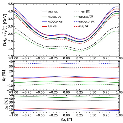
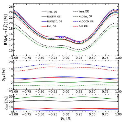
Figure 12: Scenario2: Upper: Tree-level (black), NLO EW (green), NLO QCD (blue) and full (red) partial width (left) and branching ratio (right) of the decay $H_{4}(=H_{a})\to\tilde{t}_{1}\tilde{t}_{2}^{*}$ as function of the complex phase $\varphi_{A_{t}}$. They are shown for the OS (full) and $\overline{\text{DR}}$ (dashed) scheme. Middle: Relative EW, QCD and EW+QCD corrections $\delta$ (see text, for definition) for the decay width (left) and branching ratio (right) in the OS (full) and $\overline{\text{DR}}$ (dashed) scheme. Lower: Relative differences $\Delta$ between the OS and $\overline{\text{DR}}$ scheme (see text, for definition) for the decay width (left) and branching ratio (right).

For the decay $H_{4}(\equiv H_{a})\to\tilde{t}_{1}\tilde{t}_{2}^{*}$, we show in the upper panels of Fig. 12 the partial decay width (left) and branching ratio (right) at tree-level (black), NLO EW (green), NLO QCD (blue), and NLO EW+QCD (red) as a function of $\varphi_{A_{t}}$, both for the OS (full) and $\overline{\text{DR}}$ (dashed) scheme . In the middle panels we show the relative NLO EW, NLO QCD and NLO EW+QCD corrections which are defined as

$$\delta_{\Gamma}=\frac{\Gamma^{\text{EW/QCD/EW+QCD}}_{{\bf Z}^{H}}-\Gamma^{\text{tree}}_{{\bf Z}^{H}}}{\Gamma^{\text{Tree}}_{{\bf Z}^{H}}}$$ (5.241)

and

$$\delta_{\text{BR}}=\frac{\mathrm{BR}^{\text{EW/QCD/EW+QCD}}_{{\bf Z}^{H}}-\mathrm{BR}^{\text{tree}}_{{\bf Z}^{H}}}{\mathrm{BR}^{\text{Tree}}_{{\bf Z}^{H}}}\;,$$ (5.242)

respectively. The lower panels display the relative differences between the OS and $\overline{\text{DR}}$ decay widths and branching ratios, $\Delta_{\Gamma}$ and $\Delta_{\text{BR}}$, as defined in Eq. (5.239) and Eq. (5.240), respectively. The corrections vary slightly with the phase $\varphi_{A_{t}}$. The EW corrections are negative in both schemes while the QCD corrections are positive and of the same order of magnitude. This shows the importance to include both types of corrections to make reliable predictions. Overall, the relative corrections $\delta$ in the $\overline{\text{DR}}$ scheme are larger than in the OS scheme. As can be inferred from the bottom left panel of Fig. 12, for $\varphi_{A_{t}}=0$, the relative difference in the partial width, $\Delta_{\Gamma}$, between the OS and $\overline{\text{DR}}$ scheme at tree level is about $37\%$ and decreases dramatically to less than $12\%$ when both the EW and the QCD corrections are included. Similar results are found for the branching ratios, presented on the right plots of Fig. 12, with smaller values of $21\%$ at tree level and $7\%$ at full one-loop order. Note that in the right hand side plots we treated the decays $H_{a}\to\tilde{t}_{1}\tilde{t}_{2}^{*}$ and $H_{a}\to\tilde{t}_{2}\tilde{t}_{1}^{*}$ at the same level of precision while all other decays are computed at the highest possible precision.

In the CP-invariant scenario the decay width of decay $H_{a}\to\tilde{t}_{1}\tilde{t}_{2}^{*}$ is equal to the one of its charge conjugate decay $H_{a}\to\tilde{t}_{2}\tilde{t}_{1}^{*}$. For non-vanishing $\varphi_{A_{t}}$, however, the CP asymmetry, defined as

$$\delta_{\text{CP}}=\frac{\Gamma(H_{a}\to\tilde{t}_{1}\tilde{t}_{2}^{*})-\Gamma(H_{a}\to\tilde{t}_{2}\tilde{t}_{1}^{*})}{\Gamma(H_{a}\to\tilde{t}_{1}\tilde{t}_{2}^{*})+\Gamma(H_{a}\to\tilde{t}_{2}\tilde{t}_{1}^{*})}\;,$$ (5.243)

is non-zero. In Fig. 13 we show the CP asymmetry as a function of $\varphi_{A_{t}}$. We see that the CP asymmetry appears already at tree-level, which results from the imaginary part of the WFR factor ${\bf Z}^{H}$ and the imaginary part of the tree-level couplings $g_{h_{i}\tilde{q}_{j}\tilde{q}_{k}^{*}}$. The relative change of the asymmetry due to loop corrections ranges between 18% and -9% in the OS scheme while in the $\overline{\text{DR}}$ scheme it is about 8% when the phase $\varphi_{A_{t}}$ is varied from $-\pi/4$ to $\pi/4$.

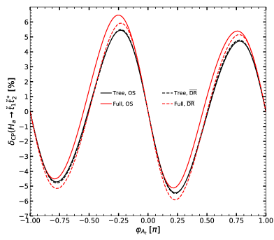
Figure 13: CP-asymmetry $\delta_{\text{CP}}$ as function of the complex phase $\varphi_{A_{t}}$ at tree level (black) and including both the EW and the QCD corrections (red) in the $\overline{\text{DR}}$ (dashed) and OS (full) scheme.

We present in Fig. 14 the same plots for the decay widths and branching ratios as in Fig. 12 but for the decay of $H_{3}\to\tilde{t}_{1}\tilde{t}_{2}^{*}$ which is the dominant decay channel of $H_{3}$. In scenario2 $H_{3}$ is $h_{d}$-like. For both the OS and the $\overline{\text{DR}}$ scheme the NLO EW corrections to the decay width are negative and the relative corrections $\delta_{\Gamma}$ are around -3% in the OS and -8% in the $\overline{\text{DR}}$ scheme. The NLO QCD corrections on the other hand are positive and their relative size can reach $8\%$ in the OS scheme and around $37\%$ in the $\overline{\text{DR}}$ scheme. For $\varphi_{A_{t}}=0$, the difference between the decay widths in the OS and the $\overline{\text{DR}}$ scheme, $\Delta_{\Gamma}$, is about $36\%$ at tree-level and reduces to 12% at full one-loop level. The corresponding numbers for the branching ratios are similar.

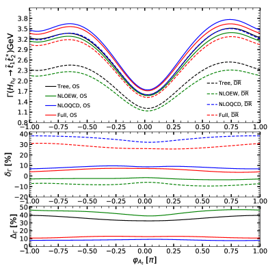
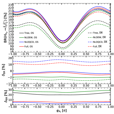
Figure 14: Similar to Fig. 12 but for the decay $H_{h_{d}}\to\tilde{t}_{1}\tilde{t}_{2}^{*}$.

We have observed that for this parameter point the EW and QCD corrections in the OS scheme are smaller in the $\overline{\text{DR}}$ scheme. In the OS scheme we have seen that this is due to a cancellation between the genuine triangle diagram contribution and the counterterm contribution while this does not happen in the $\overline{\text{DR}}$ scheme. Overall the inclusion of the QCD corrections in addition to the EW corrections reduces the difference between the OS and $\overline{\text{DR}}$ results.

6 Conclusions

In this paper, we have presented in the framework of the CP-violating NMSSM our calculation of the complete (SUSY-)EW to the on-shell Higgs boson decays into fermion pairs, massive gauge boson final states, gauge and Higgs boson final state pairs, electroweakino and stop and sbottom pairs. Where applicable we have included the SUSY-QCD corrections. We have implemented these new corrections into NMSSMCALC, a Fortran code for the computation of the Higgs mass spectrum up to presently two-loop order ${\cal O}(\alpha_{t}\alpha_{s}+\alpha_{t}^{2})$ and the calculation of their branching ratios. The code already included in the branching ratios the state-of-the-art QCD corrections and the $\Delta_{b}$ corrections as well as decays into off-shell massive gauge boson pairs and decays with off-shell heavy quarks in the final state. The new code is called NMSSMCALCEW.

The consistent implementation of our newly computed corrections provides the presently highest level of precision in the calculation of the NMSSM Higgs boson decays. In contrast to the previous NMSSMCALC version, we have included the ${\bf Z}^{H}$ factor with full momentum dependence in order to render the loop-corrected masses on-shell. For the decays into the electroweakinos and into squark pairs different renormalization schemes were implemented. The numerical analysis has demonstrated that the relative change in the branching ratios due to this new treatment and the newly implemented corrections is significant. The analysis of the decays into chargino/neutralino and squark pairs for different renormalization schemes has shown that the one-loop corrections reduce the theoretical uncertainty due to missing higher-order corrections. The new code NMSSMCALCEW can be obtained at the url:
https://www.itp.kit.edu/$\sim$maggie/NMSSMCALCEW/.

Appendix A Counterterm contribution to the decay of a neutral Higgs boson into a squark pair

In this appendix, we give explicit expressions of the counterterm couplings for the decays of a neutral Higgs boson into a squark pair. Note that we have used the redefined WFR constants for the squarks given in Eqs. (3.125) and (3.126). For the EW corrections, the counterterm entering Eq. (4.216) for the Higgs decay into a stop pair is given by

$${\cal M}^{\text{CT ,EW}}_{h_{i}\tilde{t}_{j}\tilde{t}_{k}^{*}} =\frac{1}{2}\sum_{i^{\prime}=1}^{5}g_{h_{i^{\prime}}\tilde{t}_{j}\tilde{t}_{k}^{*}}\delta Z_{h_{i}h_{i^{\prime}}}+\frac{1}{2}\sum_{j^{\prime}=1}^{2}\left(g_{h_{i}\tilde{t}_{j^{\prime}}\tilde{t}_{k}^{*}}\delta Z_{\tilde{t}_{j^{\prime}}\tilde{t}_{j}}(M_{\tilde{t}_{j}}^{2})+g_{h_{i}\tilde{t}_{j}\tilde{t}_{j^{\prime}}^{*}}\delta Z^{*}_{\tilde{t_{j^{\prime}}}\tilde{t}_{k}}(M_{\tilde{t}_{k}}^{2})\right)$$

$$+g_{h_{i}\tilde{t}_{j}\tilde{t}_{k}^{*}}\left(\delta Z_{e}+\frac{\delta M_{Z}^{2}}{2M_{Z}^{2}}-\frac{\delta s_{\theta_{W}}}{s_{\theta_{W}}}-\frac{\delta c_{\theta_{W}}}{c_{\theta_{W}}}\right)$$

$$+\frac{eM_{Z}}{s_{\theta_{W}}c_{\theta_{W}}}\bigg{[}\frac{m_{t}^{2}{\cal R}_{i2}\left(U_{j1}^{\tilde{t}*}U_{k1}^{\tilde{t}}+U_{j2}^{\tilde{t}*}U_{k2}^{\tilde{t}}\right)}{{s_{\beta}}M_{Z}^{2}}\left(2\frac{\delta m_{t}}{m_{t}}-\frac{\delta M_{Z}^{2}}{M_{Z}^{2}}-\frac{\delta{s_{\beta}}}{{s_{\beta}}}\right)$$

$$+\frac{m_{t}\left(U_{j2}^{\tilde{t}*}U_{k1}^{\tilde{t}}F_{1}+U_{j1}^{\tilde{t}*}U_{k2}^{\tilde{t}}F_{1}^{*}\right)}{2{s_{\beta}}M_{Z}^{2}}\left(\frac{\delta m_{t}}{m_{t}}-\frac{\delta M_{Z}^{2}}{M_{Z}^{2}}-\frac{\delta{s_{\beta}}}{{s_{\beta}}}\right)$$

$$+\frac{m_{t}\left(U_{j2}^{\tilde{t}*}U_{k1}^{\tilde{t}}\delta F_{1}+U_{j1}^{\tilde{t}*}U_{k2}^{\tilde{t}}\delta F_{1}^{*}\right)}{2{s_{\beta}}M_{Z}^{2}}$$

$$+\frac{1}{6}\left(\delta{c_{\beta}}{\cal R}_{i1}-\delta{s_{\beta}}{\cal R}_{i2}\right)\left((4c_{\theta_{W}}^{2}-1)U_{j1}^{\tilde{t}*}U_{k1}^{\tilde{t}}+4s_{\theta_{W}}^{2}U_{j2}^{\tilde{t}*}U_{k2}^{\tilde{t}}\right)$$

$$+\frac{4}{3}\left({c_{\beta}}{\cal R}_{i1}-{s_{\beta}}{\cal R}_{i2}\right)\left(-U_{j1}^{\tilde{t}*}U_{k1}^{\tilde{t}}+U_{j2}^{\tilde{t}*}U_{k2}^{\tilde{t}}\right)s_{\theta_{W}}\delta s_{\theta_{W}}\bigg{]},$$ (A.244)

and for the decay into a sbottom pair

$${\cal M}^{\text{CT,EW}}_{h_{i}\tilde{b}_{j}\tilde{b}_{k}^{*}} =\frac{1}{2}\sum_{i^{\prime}=1}^{5}g_{h_{i^{\prime}}\tilde{b}_{j}\tilde{b}_{k}^{*}}\delta Z_{h_{i}h_{i^{\prime}}}+\frac{1}{2}\sum_{j^{\prime}=1}^{2}\left(g_{h_{i}\tilde{b}_{j^{\prime}}\tilde{b}_{k}^{*}}\delta Z_{\tilde{b}_{j^{\prime}}\tilde{b}_{j}}(M_{\tilde{b}_{j}}^{2})+g_{h_{i}\tilde{b}_{j}\tilde{b}_{j^{\prime}}^{*}}\delta Z^{*}_{\tilde{b_{j^{\prime}}}\tilde{b}_{k}}(M_{\tilde{b}_{k}}^{2})\right)$$

$$+g_{h_{i}\tilde{b}_{j}\tilde{b}_{k}^{*}}\left(\delta Z_{e}+\frac{\delta M_{Z}^{2}}{2M_{Z}^{2}}-\frac{\delta s_{\theta_{W}}}{s_{\theta_{W}}}-\frac{\delta c_{\theta_{W}}}{c_{\theta_{W}}}\right)$$

$$+\frac{eM_{Z}}{s_{\theta_{W}}c_{\theta_{W}}}\bigg{[}\frac{m_{b}^{2}{\cal R}_{i1}\left(U_{j1}^{\tilde{b}*}U_{k1}^{\tilde{b}}+U_{j2}^{\tilde{b}*}U_{k2}^{\tilde{b}}\right)}{{c_{\beta}}M_{Z}^{2}}\left(2\frac{\delta m_{b}}{m_{b}}-\frac{\delta M_{Z}^{2}}{M_{Z}^{2}}-\frac{\delta{c_{\beta}}}{{c_{\beta}}}\right)$$

$$+\frac{m_{b}\left(U_{j2}^{\tilde{b}*}U_{k1}^{\tilde{b}}F_{2}+U_{j1}^{\tilde{b}*}U_{k2}^{\tilde{b}}F_{2}^{*}\right)}{2{c_{\beta}}M_{Z}^{2}}\left(\frac{\delta m_{b}}{m_{b}}-\frac{\delta M_{Z}^{2}}{M_{Z}^{2}}-\frac{\delta{c_{\beta}}}{{c_{\beta}}}\right)$$

$$+\frac{m_{b}\left(U_{j2}^{\tilde{b}*}U_{k1}^{\tilde{b}}\delta F_{2}+U_{j1}^{\tilde{b}*}U_{k2}^{\tilde{b}}\delta F_{2}^{*}\right)}{2{c_{\beta}}M_{Z}^{2}}$$

$$-\frac{1}{6}\left(\delta{c_{\beta}}{\cal R}_{i1}-\delta{s_{\beta}}{\cal R}_{i2}\right)\left((2c_{\theta_{W}}^{2}+1)U_{j1}^{\tilde{b}*}U_{k1}^{\tilde{b}}+2s_{\theta_{W}}^{2}U_{j2}^{\tilde{b}*}U_{k2}^{\tilde{b}}\right)$$

$$-\frac{2}{3}\left({c_{\beta}}{\cal R}_{i1}-{s_{\beta}}{\cal R}_{i2}\right)\left(-U_{j1}^{\tilde{b}*}U_{k1}^{\tilde{b}}+U_{j2}^{\tilde{b}*}U_{k2}^{\tilde{b}}\right)s_{\theta_{W}}\delta s_{\theta_{W}}\bigg{]},$$ (A.245)

where

$$\delta F_{1} =\delta A_{t}^{*}e^{-i\varphi_{u}}\left({\cal R}_{i2}-i{c_{\beta}}{\cal R}_{i4}\right)-\delta\mu_{\text{eff}}\left({\cal R}_{i1}+i{s_{\beta}}{\cal R}_{i4}\right)$$

$$-\frac{v\lambda{c_{\beta}}\left({\cal R}_{i3}+i{\cal R}_{i5}\right)e^{i\varphi_{s}}}{\sqrt{2}}\left(\frac{\delta\lambda}{\lambda}+\frac{\delta v}{v}+\frac{\delta{c_{\beta}}}{{c_{\beta}}}\right),$$ (A.246)

$$\delta F_{2} =\delta A_{b}^{*}\left({\cal R}_{i1}-i{s_{\beta}}{\cal R}_{i4}\right)-\delta\mu_{\text{eff}}e^{i\varphi_{u}}\left({\cal R}_{i2}+i{c_{\beta}}{\cal R}_{i4}\right)$$

$$-\frac{v\lambda{s_{\beta}}\left({\cal R}_{i3}+i{\cal R}_{i5}\right)e^{i(\varphi_{s}+\varphi_{u})}}{\sqrt{2}}\left(\frac{\delta\lambda}{\lambda}+\frac{\delta v}{v}+\frac{\delta{s_{\beta}}}{{s_{\beta}}}\right).$$ (A.247)

For the QCD corrections, the counterterm couplings are obtained from ${\cal M}^{\text{CT,EW}}_{h_{i}\tilde{q}_{j}\tilde{q}_{k}^{*}}$ by setting the set of EW counterterms, $\delta Z_{e},\delta M_{Z}^{2},\delta v,\delta v_{s},\delta\lambda,\delta s_{\theta_{W}},\delta c_{\theta_{W}},\delta{s_{\beta}},\delta{c_{\beta}}$ and $\delta Z_{h_{i}h_{i^{\prime}}}$ to zero. Note that the counterterm $\delta\mu_{\text{eff}}$ is given in terms of $\delta\lambda$ and $\delta v_{s}$ as

$$\delta\mu_{\text{eff}}=e^{i\varphi_{s}}\frac{(v_{s}\delta\lambda+\lambda\delta v_{s})}{\sqrt{2}}.$$ (A.248)

Appendix B The Code NMSSMCALCEW

We here give a brief introduction into our new code NMSSMCALCEW that includes the newly calculated and here presented corrections to the decay widths of the neutral NMSSM Higgs bosons in the CP-violating NMSSM, as well as the newly calculated and here presented one-loop corrections to the chargino, neutralino, stop, and sbottom masses. It is derived from the code NMSSMCALC, which is described in detail in Ref. [13]. We here concentrate on the new features in NMSSMCALCEW with respect to NMSSMCALC.

NMSSMCALCEW requires ’LoopTools’ version 2.14 (or higher) [84, 85] to work with the EW corrections in the decay part. If ’LoopTools’ is not installed yet, it can be obtained from the url: http://www.feynarts.de/looptools/

In order to generate the executable, download and unpack the tar file ’nmssmcalcew.tar.gz’. It contains two subdirectories called ’nmssmcalc_rew_alphat2-master’ and ’nmssmcalc_cew_alphat2-master’ for the real and complex NMSSM, respectively. Go to the subdirectory of the version in which you want to work in. Open in a text editor the file ’makefile’ and in line 31 provide the absolute path to the ’LoopTools’ binary directory located in the main directory of LoopTools. Modify also the line 66 (to make sure it refers to the correct ’lib’ sub-directory within the ’LoopTools’ binary directory). In case the package is compiled without the EW corrections in the decay widths, the flag ’yesEW’ can be switched to ’FALSE’ on line 19 and ’LoopTools’ is not needed anymore. Subsequently, all files are compiled by typing ’make’. An executable ’run’ is created. By typing’./run’ the executable is run.

For the code to be run, the user has to provide the input files for ’CalcMasses.F’ (default name ’inp.dat’) and for bhdecay(_c).f (to be named ’bhdecay.in’). The user also has the choice to provide in the command line the names of the input and output files for ’CalcMasses.F’ (first and second argument) and the name of the output file provided by the decay routine (third argument). Hence the command will be ’run name_file1 name_file2 name_file3’ in this case. Sample input files ’inp.dat’ and ’bhdecay.in’ are included in the .tar files. By typing ’make clean’ the executable as well as the object files generated in the ’obj’ directory are removed.

In ’bhdecay.in’ that is used by NMSSMCALCEW, new options have been included. They are

• ’ischhXX’ to choose the renormalization scheme for the loop corrected electroweakino masses. The options are 1 (OS1), 2 (OS2) and 3 (DRbar). The two OS schemes are specified in Section 3.1.2.

• ’ischhst’ to choose the renormalization scheme for the stop sector. The options are 1 (OS NLO-EW, OS NLO-QCD), 2 (OS NLO-EW, DRbar NLO-QCD), 3 (DRbar NLO-EW, DRbar NLO-QCD).

• ’ischhsb’ to choose the renormalization scheme for the sbottom sector. The options are 1 (OS NLO-EW, OS NLO-QCD), 2 (OS NLO-EW, DRbar NLO-QCD), 3 (DRbar NLO-EW, DRbar NLO-QCD).

• ’iewh’ to choose the levels of NLO SUSY-EW (SUSY-QCD) corrections that are included. The options are 0 (as in NMSSMCALC 3.00), 1 (decays as implemented in NMSSMCALC, but with the ${\bf Z}^{H}$ factor), 2 (full NLO corrections as described in this paper). Both for option 1 and 2, the loop-corrected electroweakino and stop/sbottom masses are used in the phase space factor.

Further information on the organization of the files for the code and their functionalities as well as modifications on the code (which are constantly updated) can be found at the webpage of NMSSMCALCEW. The code has been tested on a Linux machine.

Acknowledgments

JB acknowledges the support from the Carl-Zeiss foundation. TND and MM acknowledge financial support from the DFG project Precision Calculations in the Higgs Sector - Paving the Way to the New Physics Landscape (ID: MU 3138/1-1). TND’s work is funded by the Vietnam National Foundation for Science and Technology Development (NAFOSTED) under grant number 103.01-2017.78.

Note added While this paper was being completed, Ref. [86] appeared, where the impact of the EW corrections to heavy Higgs boson decays into fermion pairs was discussed. It was shown that these contributions are dominated by Sudakov double logarithms. The authors furthermore stressed the relevance of three-body decays for a consistent evaluation of the total widths and branching ratios at complete one-loop order.

References

- [1] ATLAS, G. Aad et al., Phys. Lett. B716, 1 (2012), 1207.7214.
- [2] CMS, S. Chatrchyan et al., Phys. Lett. B716, 30 (2012), 1207.7235.
- [3] ATLAS, CMS, G. Aad et al., Phys. Rev. Lett. 114, 191803 (2015), 1503.07589.
- [4] M. Maniatis, Int. J. Mod. Phys. A25, 3505 (2010), 0906.0777.
- [5] U. Ellwanger, C. Hugonie, and A. M. Teixeira, Phys. Rept. 496, 1 (2010), 0910.1785.
- [6] J. Baglio, C. O. Krauss, M. Mühlleitner, and K. Walz, JHEP 10, 024 (2015), 1505.07125.
- [7] G. Bélanger, V. Bizouard, F. Boudjema, and G. Chalons, Phys. Rev. D93, 115031 (2016), 1602.05495.
- [8] G. Bélanger, V. Bizouard, F. Boudjema, and G. Chalons, Phys. Rev. D96, 015040 (2017), 1705.02209.
- [9] M. D. Goodsell, S. Liebler, and F. Staub, (2017), 1703.09237.
- [10] F. Domingo, S. Heinemeyer, S. Paßehr, and G. Weiglein, Eur. Phys. J. C78, 942 (2018), 1807.06322.
- [11] D. T. Nhung, M. Mühlleitner, J. Streicher, and K. Walz, JHEP 1311, 181 (2013), 1306.3926.
- [12] M. Mühlleitner, D. T. Nhung, and H. Ziesche, JHEP 12, 034 (2015), 1506.03321.
- [13] J. Baglio et al., Comput. Phys. Commun. 185, 3372 (2014), 1312.4788.
- [14] K. Ender, T. Graf, M. Mühlleitner, and H. Rzehak, Phys. Rev. D85, 075024 (2012), 1111.4952.
- [15] T. Graf, R. Gröber, M. Mühlleitner, H. Rzehak, and K. Walz, JHEP 10, 122 (2012), 1206.6806.
- [16] M. Mühlleitner, D. T. Nhung, H. Rzehak, and K. Walz, JHEP 1505, 128 (2015), 1412.0918.
- [17] T. N. Dao, R. Gröber, M. Krause, M. Mühlleitner, and H. Rzehak, (2019), 1903.11358.
- [18] M. Kobayashi and T. Maskawa, Prog. Theor. Phys. 49, 652 (1973).
- [19] A. Bharucha, A. Fowler, G. Moortgat-Pick, and G. Weiglein, JHEP 05, 053 (2013), 1211.3134.
- [20] D. Espriu, J. Manzano, and P. Talavera, Phys. Rev. D66, 076002 (2002), hep-ph/0204085.
- [21] A. C. Fowler and G. Weiglein, JHEP 01, 108 (2010), 0909.5165.
- [22] A. Denner, Fortsch. Phys. 41, 307 (1993), 0709.1075.
- [23] T. Fritzsche and W. Hollik, Eur. Phys. J. C24, 619 (2002), hep-ph/0203159.
- [24] J. Guasch, W. Hollik, and J. Sola, JHEP 10, 040 (2002), hep-ph/0207364.
- [25] N. Baro and F. Boudjema, Phys. Rev. D80, 076010 (2009), 0906.1665.
- [26] A. Chatterjee, M. Drees, S. Kulkarni, and Q. Xu, Phys. Rev. D85, 075013 (2012), 1107.5218.
- [27] K. Williams and G. Weiglein, Phys. Lett. B660, 217 (2008), 0710.5320.
- [28] D. Pierce and A. Papadopoulos, Phys. Rev. D50, 565 (1994), hep-ph/9312248.
- [29] H. Eberl, M. Kincel, W. Majerotto, and Y. Yamada, Phys. Rev. D64, 115013 (2001), hep-ph/0104109.
- [30] S. P. Martin, Phys. Rev. D72, 096008 (2005), hep-ph/0509115.
- [31] J. Küblbeck, M. Böhm, and A. Denner, Comput. Phys. Commun. 60, 165 (1990).
- [32] T. Hahn, Comput. Phys. Commun. 140, 418 (2001), hep-ph/0012260.
- [33] F. Staub, Comput. Phys. Commun. 181, 1077 (2010), 0909.2863.
- [34] F. Staub, Comput. Phys. Commun. 182, 808 (2011), 1002.0840.
- [35] F. Staub, Computer Physics Communications 184, pp. 1792 (2013), 1207.0906.
- [36] F. Staub, Comput. Phys. Commun. 185, 1773 (2014), 1309.7223.
- [37] R. Mertig, M. Böhm, and A. Denner, Comput. Phys. Commun. 64, 345 (1991).
- [38] V. Shtabovenko, R. Mertig, and F. Orellana, Comput. Phys. Commun. 207, 432 (2016), 1601.01167.
- [39] T. Hahn and M. Perez-Victoria, Comput. Phys. Commun. 118, 153 (1999), hep-ph/9807565.
- [40] M. Carena, D. Garcia, U. Nierste, and C. E. M. Wagner, Nucl. Phys. B577, 88 (2000), hep-ph/9912516.
- [41] M. Carena, J. R. Ellis, S. Mrenna, A. Pilaftsis, and C. E. M. Wagner, Nucl. Phys. B659, 145 (2003), hep-ph/0211467.
- [42] J. Guasch, P. Hafliger, and M. Spira, Phys. Rev. D68, 115001 (2003), hep-ph/0305101.
- [43] R. Hempfling, Phys.Rev. D49, 6168 (1994).
- [44] L. J. Hall, R. Rattazzi, and U. Sarid, Phys. Rev. D50, 7048 (1994), hep-ph/9306309.
- [45] M. Carena, M. Olechowski, S. Pokorski, and C. Wagner, Nucl.Phys. B426, 269 (1994), hep-ph/9402253.
- [46] D. M. Pierce, J. A. Bagger, K. T. Matchev, and R.-j. Zhang, Nucl. Phys. B491, 3 (1997), hep-ph/9606211.
- [47] M. Carena, S. Mrenna, and C. E. M. Wagner, Phys. Rev. D60, 075010 (1999), hep-ph/9808312.
- [48] D. Noth and M. Spira, Phys.Rev.Lett. 101, 181801 (2008), 0808.0087.
- [49] L. Mihaila and C. Reisser, JHEP 1008, 021 (2010), 1007.0693.
- [50] E. Braaten and J. P. Leveille, Phys. Rev. D22, 715 (1980).
- [51] N. Sakai, Phys. Rev. D22, 2220 (1980).
- [52] T. Inami and T. Kubota, Nucl. Phys. B179, 171 (1981).
- [53] M. Drees and K.-i. Hikasa, Phys. Lett. B240, 455 (1990), [Erratum: Phys. Lett.B262,497(1991)].
- [54] D. Yu. Bardin, P. K. Khristova, and B. M. Vilensky, Sov. J. Nucl. Phys. 54, 833 (1991), [Yad. Fiz.54,1366(1991)].
- [55] A. Dabelstein and W. Hollik, Z. Phys. C53, 507 (1992).
- [56] A. Dabelstein, Nucl. Phys. B456, 25 (1995), hep-ph/9503443.
- [57] A. Djouadi, J. Kalinowski, and M. Spira, Comput. Phys. Commun. 108, 56 (1998), hep-ph/9704448.
- [58] A. Djouadi, J. Kalinowski, M. Muehlleitner, and M. Spira, Comput. Phys. Commun. 238, 214 (2019), 1801.09506.
- [59] M. Drees and K.-i. Hikasa, Phys. Rev. D41, 1547 (1990).
- [60] S. G. Gorishnii, A. L. Kataev, S. A. Larin, and L. R. Surguladze, Mod. Phys. Lett. A5, 2703 (1990).
- [61] S. G. Gorishnii, A. L. Kataev, S. A. Larin, and L. R. Surguladze, Phys. Rev. D43, 1633 (1991).
- [62] A. L. Kataev and V. T. Kim, Mod. Phys. Lett. A9, 1309 (1994).
- [63] S. G. Gorishnii, A. L. Kataev, and S. A. Larin, Sov. J. Nucl. Phys. 40, 329 (1984), [Yad. Fiz.40,517(1984)].
- [64] L. R. Surguladze, Phys. Lett. B341, 60 (1994), hep-ph/9405325.
- [65] S. A. Larin, T. van Ritbergen, and J. A. M. Vermaseren, Phys. Lett. B362, 134 (1995), hep-ph/9506465.
- [66] K. G. Chetyrkin and A. Kwiatkowski, Nucl. Phys. B461, 3 (1996), hep-ph/9505358.
- [67] K. G. Chetyrkin, Phys. Lett. B390, 309 (1997), hep-ph/9608318.
- [68] P. A. Baikov, K. G. Chetyrkin, and J. H. Kuhn, Phys. Rev. Lett. 96, 012003 (2006), hep-ph/0511063.
- [69] K. E. Williams, H. Rzehak, and G. Weiglein, Eur. Phys. J. C71, 1669 (2011), 1103.1335.
- [70] B. A. Kniehl, Nucl. Phys. B357, 439 (1991).
- [71] P. Gonzalez, S. Palmer, M. Wiebusch, and K. Williams, Eur. Phys. J. C73, 2367 (2013), 1211.3079.
- [72] T. N. Dao, L. Fritz, M. Krause, M. Muhlleitner, and S. Patel, To appear .
- [73] W. Hollik and J.-H. Zhang, Phys. Rev. D84, 055022 (2011), 1109.4781.
- [74] P. Bechtle, O. Brein, S. Heinemeyer, G. Weiglein, and K. E. Williams, Comput. Phys. Commun. 181, 138 (2010), 0811.4169.
- [75] P. Bechtle, O. Brein, S. Heinemeyer, G. Weiglein, and K. E. Williams, Comput. Phys. Commun. 182, 2605 (2011), 1102.1898.
- [76] P. Bechtle et al., Eur. Phys. J. C74, 2693 (2014), 1311.0055.
- [77] P. Bechtle, S. Heinemeyer, O. Stål, T. Stefaniak, and G. Weiglein, Eur. Phys. J. C74, 2711 (2014), 1305.1933.
- [78] J. Baglio et al., EPJ Web Conf. 49, 12001 (2013).
- [79] Particle Data Group, M. Tanabashi et al., Phys. Rev. D 98, 030001 (2018).
- [80] A. Denner et al., (2015), LHCHXSWG-INT-2015-006.
- [81] P. Z. Skands et al., JHEP 07, 036 (2004), hep-ph/0311123.
- [82] CMS, V. Khachatryan et al., Phys. Lett. B755, 217 (2016), 1510.01181.
- [83] CMS, V. Khachatryan et al., Phys. Lett. B759, 369 (2016), 1603.02991.
- [84] G. J. van Oldenborgh and J. A. M. Vermaseren, Z. Phys. C46, 425 (1990).
- [85] T. Hahn and M. Perez-Victoria, Comput. Phys. Commun. 118, 153 (1999), hep-ph/9807565.
- [86] F. Domingo and S. Paßehr, (2019), 1907.05468.