A Hybrid Neural Network Model for Commonsense Reasoning

Abstract

This paper proposes a hybrid neural network (HNN) model for commonsense reasoning. An HNN consists of two component models, a masked language model and a semantic similarity model, which share a BERT-based contextual encoder but use different model-specific input and output layers. HNN obtains new state-of-the-art results on three classic commonsense reasoning tasks, pushing the WNLI benchmark to 89%, the Winograd Schema Challenge (WSC) benchmark to 75.1%, and the PDP60 benchmark to 90.0%. An ablation study shows that language models and semantic similarity models are complementary approaches to commonsense reasoning, and HNN effectively combines the strengths of both. The code and pre-trained models will be publicly available at https://github.com/namisan/mt-dnn.

1 Introduction

Commonsense reasoning is fundamental to natural language understanding (NLU). As shown in the examples in Table 1, in order to infer what the pronoun “they” refers to in the first two statements, one has to leverage the commonsense knowledge that “demonstrators usually cause violence and city councilmen usually fear violence.” Similarly, it is obvious to humans what the pronoun “it” refers to in the third and fourth statements due to the commonsense knowledge that “An object cannot fit in a container because either the object (trophy) is too big or the container (suitcase) is too small.”

1. The city councilmen refused the demonstrators a permit because they feared violence. Who feared violence?
   A. The city councilmen    B. The demonstrators

2. The city councilmen refused the demonstrators a permit because they advocated violence. Who advocated violence?
   A. The city councilmen    B. The demonstrators

3. The trophy doesn’t fit in the brown suitcase because it is too big. What is too big?
   A. The trophy    B. The suitcase

4. The trophy doesn’t fit in the brown suitcase because it is too small. What is too small?
   A. The trophy    B. The suitcase

Table 1: Examples from Winograd Schema Challenge (WSC). The task is to identify the reference of the pronoun in bold.

In this paper, we study two classic commonsense reasoning tasks: the Winograd Schema Challenge (WSC) and Pronoun Disambiguation Problem (PDP) Levesque et al. (2011); Davis and Marcus (2015). Both tasks are formulated as an anaphora resolution problem, which is a form of co-reference resolution, where a machine (AI agent) must identify the antecedent of an ambiguous pronoun in a statement. WSC and PDP differ from other co-reference resolution tasks Soon et al. (2001); Ng and Cardie (2002); Peng et al. (2016) in that commonsense knowledge, which cannot be explicitly decoded from the given text, is needed to solve the problem, as illustrated in the examples in Table 1.

Comparing with other commonsense reasoning tasks, such as COPA Roemmele et al. (2011), Story Cloze Test Mostafazadeh et al. (2016), Event2Mind Rashkin et al. (2018), SWAG Zellers et al. (2018), ReCoRD Zhang et al. (2018), and so on, WSC and PDP better approximate real human reasoning, can be easily solved by native English-speaker Levesque et al. (2011), and yet are challenging for machines. For example, the WNLI task, which is derived from WSC, is considered the most challenging NLU task in the General Language Understanding Evaluation (GLUE) benchmark Wang et al. (2018). Most machine learning models can hardly outperform the naive baseline of majority voting (scored at 65.1) , including BERT Devlin et al. (2018a) and Distilled MT-DNN Liu et al. (2019a).

While traditional methods of commonsense reasoning rely heavily on human-crafted features and knowledge bases Rahman and Ng (2012a); Sharma et al. (2015); Schüller (2014); Bailey et al. (2015); Liu et al. (2017), we explore in this study machine learning approaches using deep neural networks (DNN). Our method is inspired by two categories of DNN models proposed recently.

The first are neural language models trained on large amounts of text data. Trinh and Le (2018) proposed to use a neural language model trained on raw text from books and news to calculate the probabilities of the natural language sentences which are constructed from a statement by replacing the to-be-resolved pronoun in the statement with each of its candidate references (antecedent), and then pick the candidate with the highest probability as the answer. Kocijan et al. (2019) showed that a significant improvement can be achieved by fine-tuning a pre-trained masked language model (BERT in their case) on a small amount of WSC labeled data.

The second category of models are semantic similarity models. Wang et al. (2019) formulated WSC and PDP as a semantic matching problem, and proposed to use two variations of the Deep Structured Similarity Model (DSSM) Huang et al. (2013) to compute the semantic similarity score between each candidate antecedent and the pronoun by (1) mapping the candidate and the pronoun and their context into two vectors, respectively, in a hidden space using deep neural networks, and (2) computing cosine similarity between the two vectors. The candidate with the highest score is selected as the result.

The two categories of models use different inductive biases when predicting outputs given inputs, and thus capture different views of the data. While language models measure the semantic coherence and wholeness of a statement where the pronoun to be resolved is replaced with its candidate antecedent, DSSMs measure the semantic relatedness of the pronoun and its candidate in their context.

Therefore, inspired by multi-task learning Caruana (1997); Liu et al. (2015, 2019b), we propose a hybrid neural network (HNN) model that combines the strengths of both neural language models and a semantic similarity model. As shown in Figure 1, HNN consists of two component models, a masked language model and a deep semantic similarity model. The two component models share the same text encoder (BERT), but use different model-specific input and output layers. The final output score is the combination of the two model scores. The architecture of HNN bears a strong resemblance to that of Multi-Task Deep Neural Network (MT-DNN) Liu et al. (2019b), which consists of a BERT-based text encoder that is shared across all tasks (models) and a set of task (model) specific output layers. Following Liu et al. (2019b); Kocijan et al. (2019), the training procedure of HNN consists of two steps: (1) pretraining the text encoder on raw text , and (2) multi-task learning of HNN on WSCR which is the most popular WSC dataset, as suggested by Kocijan et al. (2019).

HNN obtains new state-of-the-art results with significant improvements on three classic commonsense reasoning tasks, pushing the WNLI benchmark in GLUE to 89%, the WSC benchmark Levesque et al. (2011) to 75.1%, and the PDP-60 benchmark to 90.0%. We also conduct an ablation study which shows that language models and semantic similarity models provide complementary approaches to commonsense reasoning, and HNN effectively combines the strengths of both.

2 The Proposed HNN Model

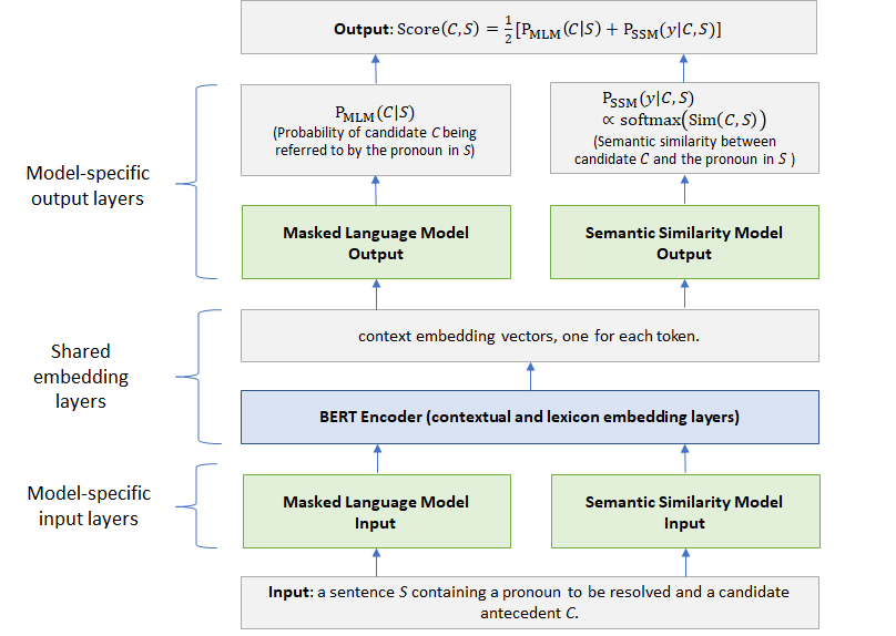
Figure 1: Architecture of the hybrid model for commonsense reasoning. The model consists of two component models, a masked language model (MLM) and a semantic similarity model (SSM). The input includes the sentence $S$, which contains a pronoun to be resolve, and a candidate antecedent $C$. The two component models share the BERT-based contextual encoder, but use different model-specific input and output layers. The final output score is the combination of the two component model scores.

The architecture of the proposed hybrid model is shown in Figure 1. The input includes a sentence $S$, which contains the pronoun to be resolved, and a candidate antecedent $C$. The two component models, masked language model (MLM) and semantic similarity model (SSM), share the BERT-based contextual encoder, but use different model-specific input and output layers. The final output score, which indicates whether $C$ is the correct candidate of the pronoun in $S$, is the combination of the two component model scores.

2.1 Masked Language Model (MLM)

This component model follows Kocijan et al. (2019). In the input layer, a masked sentence is constructed using $S$ by replacing the to-be-resolved pronoun in $S$ with a sequence of $N$ [MASK] tokens, where $N$ is the number of tokens in candidate $C$.

In the output layer, the likelihood of $C$ being referred to by the pronoun in $S$ is scored using the BERT-based masked language model $P_{mlm}(C|S)$. If $C=\{c_{1}...c_{N}\}$ consists of multiple tokens, $\log P_{mlm}(C|S)$ is computed as the average of log-probabilities of each composing token:

$$P_{mlm}(C|S)=\exp{\left(\frac{1}{N}\sum_{k=1...N}\log P_{mlm}(c_{k}|S)\right)}.$$ (1)

2.2 Semantic Similarity Model (SSM)

In the input layer, we treat sentence $S$ and candidate $C$ as a pair $(S,C)$ that is packed together as a word sequence, where we add the [CLS] token as the first token and the [SEP] token between $S$ and $C$.

After applying the shared embedding layers, we obtain the semantic representations of $S$ and $C$, denoted as $\mathbf{s}\in\mathbb{R}^{d}$ and $\mathbf{c}\in\mathbb{R}^{d}$, respectively. We use the contextual embedding of [CLS] as $\mathbf{s}$. Suppose $C$ consists of $N$ tokens, whose contextual embeddings are $\mathbf{h}_{1},...,\mathbf{h}_{N}$, respectively. The semantic representation of the candidate $C$, $\mathbf{c}$, is computed via attention as follows:

$$\alpha_{k}=\text{softmax}(\frac{\mathbf{s}^{\top}\mathbf{W}_{1}\mathbf{h}_{k}}{\sqrt{d}}),$$ (2)

$$\mathbf{c}=\sum_{k=1...N}{\alpha_{k}\cdot\mathbf{h}_{k}}.$$ (3)

where $\mathbf{W}_{1}$ is a learnable parameter matrix, and $\alpha$ is the attention score.

We use the contextual embedding of the first token of the pronoun in $S$ as the semantic representation of the pronoun, denoted as $\mathbf{p}\in\mathbb{R}^{d}$. In the output layer, the semantic similarity between the pronoun and the context is computed using a bilinear model:

$$\text{Sim}(C,S)=\mathbf{p}^{\top}\mathbf{W}_{2}\mathbf{c},$$ (4)

where $\mathbf{W}_{2}$ is a learnable parameter matrix. Then, SSM predicts whether $C$ is a correct candidate (i.e., $(C,S)$ is a positive pair, labeled as $y=1$) using the logistic function:

$$P_{ssm}(y=1|C,S)=\frac{1}{1+\exp{(-\text{Sim}(C,S))}}.$$ (5)

The final output score of pair $(S,C)$ is a linear combination of the MLM score of Eqn. 1 and the SSM score of Eqn. 5:

$$\text{Score}(C,S)=\frac{1}{2}[P_{mlm}(C|S)+P_{ssm}(y=1|C,S)].$$ (6)

2.3 The Training Procedure

We train our model of Figure 1 on the WSCR dataset, which consists of 1886 sentences, each being paired with a positive candidate antecedent and a negative candidate.

The shared BERT encoder is initialized using the published BERT uncased large model Devlin et al. (2018a). We then finetune the model on the WSCR dataset by optimizing the combined objectives:

$$\mathcal{L}_{mlm}+\mathcal{L}_{ssm}+\mathcal{L}_{rank},$$ (7)

where $\mathcal{L}_{mlm}$ is the negative log-likelihood based on the masked language model of Eqn. 1, and $\mathcal{L}_{ssm}$ is the cross-entropy loss based on semantic similarity model of Eqn. 5.

$\mathcal{L}_{rank}$ is the pair-wise rank loss. Consider a sentence $S$ which contains a pronoun to be resolved, and two candidates $C^{+}$ and $C^{-}$, where $C^{+}$ is correct and $C^{-}$ is not. We want to maximize $\Delta=\text{Score}(S,C^{+})-\text{Score}(S,C^{-})$, where Score(.) is defined by Eqn. 6. We achieve this via optimizing a smoothed rank loss:

$$\mathcal{L}_{rank}=\log(1+\exp{(-\gamma(\Delta+\beta))}),$$ (8)

where $\gamma\in[1,10]$ is the smoothing factor and $\beta\in[0,1]$ the margin hyperparameter. In our experiments, the default setting is $\gamma=10$, and $\beta=0.6$.

3 Experiments

We evaluate the proposed HNN on three commonsense benchmarks: WSC Levesque et al. (2012), PDP60 and WNLI. WNLI is derived from WSC, and is considered the most challenging NLU task in the GLUE benchmark Wang et al. (2018).

3.1 Datasets

Corpus	#Train	#Dev	#Test
WNLI	-	634 + 71	146
PDP60	-	-	60
WSC	-	-	285
WSCR	1322	564	-

Table 2: Summary of the three benchmark datasets: WSC, PDP60 and WNLI, and the additional dataset WSCR. Note that we only use WSCR for training. For WNLI, we merge its official training set containing 634 instances and dev set containing 71 instances as its final dev set.

Table 2 summarizes the datasets which are used in our experiments. Since the WSC and PDP60 datasets do not contain any training instances, following Kocijan et al. (2019), we adopt the WSCR dataset Rahman and Ng (2012b) for model training and selection. WSCR contains 1886 instances (1322 for training and the rest as dev set). Each instance is presented using the same structure as that in WSC.

For the WNLI instances, we convert them to the format of WSC as illustrated in Table 3: we first detect pronouns in the premise using spaCy; then given the detected pronoun, we search its left of the premise in hypothesis to find the longest common substring (LCS) ignoring character case. Similarly, we search its right part to the LCS; by comparing the indexes of the extracted LSCs, we extract the candidate. A detailed example of the conversion process is provided in Table 3.

1. Premise: The cookstove was warming the kitchen, and the lamplight made it seem even warmer.
   Hypothesis: The lamplight made the cookstove seem even warmer.
   Index of LCS in the hypothesis: left[0, 2], right[5, 7]
   Candidate: [3, 4] (the cookstove)

2. Premise: The cookstove was warming the kitchen, and the lamplight made it seem even warmer.
   Hypothesis: The lamplight made the kitchen seem even warmer.
   Index of LCS in the hypothesis: left[0, 2], right[5, 7]
   Candidate: [3, 4] (the kitchen)

3. Premise: The cookstove was warming the kitchen, and the lamplight made it seem even warmer.
   Hypothesis: The lamplight made the lamplight seem even warmer.
   Index of LCS in the hypothesis: left[0, 2], right[5, 7]
   Candidate: [3, 4] (the lamplight)

4. Converted: The cookstove was warming the kitchen, and the lamplight made it seem even warmer.
   A. the cookstove   B. the kitchen    C. the lamplight

Table 3: Examples of transforming WNLI to WSC format. Note that the text highlighted by brown is the longest common substring from the left part of pronoun it, and the text highlighted by violet is the longest common substring from its right.

3.2 Implementation Detail

Our implementation of HNN is based on the PyTorch implementation of BERT. All the models are trained with hyper-parameters depicted as follows unless stated otherwise. The shared layer is initialized by the BERT uncased large model. Adam Kingma and Ba (2014) is used as our optimizer with a learning rate of 1e-5 and a batch size of 32 or 16. The learning rate is linearly decayed during training with 100 warm up steps. We select models based on the dev set by greedily searching epochs between 8 and 10. The trainable parameters, e.g., $\mathbf{W_{1}}$ and $\mathbf{W_{2}}$, are initialized by a truncated normal distribution with a mean of $0$ and a standard deviation of $0.01$. The margin hyperparameter, $\beta$ in Eqn. 8, is set to 0.6 for MLM and 0.5 for SSM, and $\gamma$ is set to 10 for all tasks. We also apply SWA Izmailov et al. (2018) to improve the generalization of models. All the texts are tokenized using WordPieces, and are chopped to spans containing 512 tokens at most.

3.3 Results

We compare our HNN with a list of state-of-the-art models in the literature, including BERT Devlin et al. (2018b), GPT-2 Radford et al. (2019) and DSSM Wang et al. (2019). The brief description of each baseline is introduced as follows.

1. BERT_LARGE-LM Devlin et al. (2018b): This is the large BERT model, and we use MLM to predict a score for each candidate following Eq 1.

2. GPT-2 Radford et al. (2019): During prediction, We first replace the pronoun in a given sentence with its candidates one by one. We use the GPT-2 model to compute a score for each new sentence after the replacement, and select the candidate with the highest score as the final prediction.

3. BERT_Wiki-WSCR and BERT_WSCR Kocijan et al. (2019): These two models use the same approach as BERT_LARGE-LM, but are trained with different additional training data. For example, BERT_Wiki-WSCR is firstly fine-tuned on the constructed Wikipedia data and then on WSCR. BERT_WSCR is directly fine-tuned on WSCR.

4. DSSM Wang et al. (2019): It is the unsupervised semantic matching model trained on the dataset generated with heuristic rules.

5. HNN: It is the proposed hybrid neural network model.

	WNLI	WSC	PDP60
DSSM Wang et al. (2019)	-	63.0	75.0
BERT${}_{\text{LARGE-LM}}$ Devlin et al. (2018a)	65.1	62.0	78.3
GPT-2 Radford et al. (2019)	-	70.7	-
BERT${}_{\text{Wiki-WSCR}}$ Kocijan et al. (2019)	71.9	72.2	-
BERT${}_{\text{WSCR}}$ Kocijan et al. (2019)	70.5	70.3	-
HNN	83.6	75.1	90.0
HNN${}_{\text{ensemble}}$	89.0	-	-

Table 4: Test results

Figure 2: Comparison with SSM and MLM on WNLI examples.

	WNLI	WSCR	WSC	PDP60
HNN	77.1	85.6	75.1	90.0
-SSM	74.5	82.4	72.6	86.7
-MLM	75.1	83.7	72.3	88.3

Table 5: Ablation study of the two component model in HNN. Note that WNLI and WSCR are reported on dev sets while WSC and PDP60 are reported on test sets.

The main results are reported in Table 4. Compared with all the baselines, HNN obtains much better performance across three benchmarks. This clearly demonstrates the advantage of the HNN over existing models. For example, HNN outperforms the previous state-of-the-art BERT${}_{\text{Wiki-WSCR}}$ model with a 11.7% absolute improvement (83.6% vs 71.9%) on WNLI and a 2.8% absolute improvement (75.1% vs 72.2%) on WSC in terms of accuracy. Meanwhile, it achieves a 11.7% absolute improvement over the previous state-of-the-art BERT${}_{\text{LARGE-LM}}$ model on PDP60 in accuracy. Note that both BERT${}_{\text{Wiki-WSCR}}$ and BERT${}_{\text{LARGE-LM}}$ are using language model-based approaches to solve the pronoun resolution problem. On the other hand, We observe that DSSM without pre-training is comparable to BERT${}_{\text{LARGE-LM}}$ which is pre-trained on the large scale text corpus (63.0% vs 62.0% on WSC and 75.0% vs 78.3% on PDP60). Our results show that HNN, combining the strengths of both DSSM and BERT${}_{\text{WSCR}}$, has consistently achieved new state-of-the-art results on all three tasks.

To further boost the WNLI accuracy on the GLUE benchmark leaderboard, we record the model prediction at each epoch, and then produce the final prediction based on the majority voting from the last six model predictions. We refer to the ensemble of six models as HNN${}_{\text{ensemble}}$ in Table 4. HNN${}_{\text{ensemble}}$ brings a 5.4% absolute improvement (89.0% vs 83.6%) on WNLI in terms of accuracy.

3.4 Ablation study

In this section, we study the importance of each component in HNN by answering following questions:

How important are the two component models: MLM and SSM?

To answer this question, we first remove each component model, either SSM or MLM, and then report the performance impact of these component models. Table 5 summarizes the experimental results. It is expected that the removal of either component model results in a significant performance drop. For example, with the removal of SSM, the performance of HNN is downgraded from 77.1% to 74.5% on WNLI. Similarly, with the removal of MLM, HNN only obtains 75.1%, which amounts to a 2% drop. All these observations clearly demonstrate that SSM and MLM are complementary to each other and the HNN model benefits from the combination of both.

Figure 2 gives several examples showing how SSM and MLM complement each other on WNLI. We see that in the first pair of examples, MLM correctly predicts the label while SSM does not. This is due to the fact that “the roof repaired” appears more frequently than “the tree repaired” in the text corpora used for model pre-training. However, in the second pair, since both “the demonstrators” and “the city councilment” could advocate violence and neither occurs significantly more often than the other, SSM is more effective in distinguishing the difference based on their context. The proposed HNN, which combines the strengths of these two models, can obtain the correct results in both cases.

Does the additional ranking loss help?

As in Eqn. 7, the training objective of HNN model contains three losses. The first two are based on the two component models, respectively, and the third one, as defined in Eqn. 8, is a ranking loss based on the score function in Eqn. 6. At first glance, the ranking loss seems redundant. Thus, we compare two versions of HNN trained with and without the ranking loss. Experimental results are shown in Table 6. We see that without the ranking loss, the performance of HNN drops on three datasets: WNLI, WSCR and WSC. On the PDP60 dataset, without the ranking loss, the model performs slightly better. However, since the test set of PDP60 includes only 60 samples, the difference is not statistically significant. Thus, we decide to always include the ranking loss in the training objective of HNN.

	WNLI	WSCR	WSC	PDP60
HNN	77.1	85.6	75.1	90.0
HNN-Rank	74.8	85.1	71.9	91.7

Table 6: Ablation study of the ranking loss. Note that WNLI and WSCR are reported on dev sets while WSC and PDP60 are reported on test sets.

Is the WNLI task a ranking or classification task?

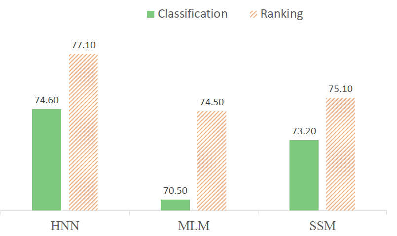
Figure 3: Comparison of different task formulation on WNLI.

The WNLI task can be formulated as either a ranking task or a classification task. To study the difference in problem formulation, we conduct experiments to compare the performance of a model used as a classifier or a ranker. For example, given a trained HNN, when it is used as a classifier we set a threshold to decide label (0/1) for each input. When it is used as a ranker, we simply pick the top-ranked candidate as the correct answer. We run the comparison using all three models HNN, MLM and SSM. As shown in Figure 3, the ranking formulation is consistently better than the classification formulation for this task. For example, the difference in the HNN model is about absolute 2.5% (74.6% vs 77.1%) in terms of accuracy.

4 Conclusion

We propose a hybrid neural network (HNN) model for commonsense reasoning. HNN consists of two component models, a masked language model and a deep semantic similarity model, which share a BERT-based contextual encoder but use different model-specific input and output layers.

HNN obtains new state-of-the-art results on three classic commonsense reasoning tasks, pushing the WNLI benchmark to 89%, the WSC benchmark to 75.1%, and the PDP60 benchmark to 90.0%. We also justify the design of HNN via a series of ablation experiments.

In future work, we plan to extend HNN to more sophisticated reasoning tasks, especially those where large-scale language models like BERT and GPT do not perform well, as discussed in Gao et al. (2019); Niven and Kao (2019).

References

- Bailey et al. (2015) Daniel Bailey, Amelia Harrison, Yuliya Lierler, Vladimir Lifschitz, and Julian Michael. 2015. The winograd schema challenge and reasoning about correlation. In Knowledge Representation; Coreference Resolution; Reasoning.
- Caruana (1997) Rich Caruana. 1997. Multitask learning. Machine learning, 28(1):41–75.
- Davis and Marcus (2015) Ernest Davis and Gary Marcus. 2015. Commonsense reasoning and commonsense knowledge in artificial intelligence. Communications of the ACM.
- Devlin et al. (2018a) Jacob Devlin, Ming-Wei Chang, Kenton Lee, and Kristina Toutanova. 2018a. Bert: Pre-training of deep bidirectional transformers for language understanding. arXiv preprint arXiv:1810.04805.
- Devlin et al. (2018b) Jacob Devlin, Ming-Wei Chang, Kenton Lee, and Kristina Toutanova. 2018b. Bert: Pre-training of deep bidirectional transformers for language understanding. arXiv preprint arXiv:1810.04805.
- Gao et al. (2019) Jianfeng Gao, Michel Galley, and Lihong Li. 2019. Neural approaches to conversational ai. Foundations and Trends® in Information Retrieval, 13(2-3):127–298.
- Huang et al. (2013) Po-Sen Huang, Xiaodong He, Jianfeng Gao, Li Deng, Alex Acero, and Larry Heck. 2013. Learning deep structured semantic models for web search using clickthrough data. In Proceedings of the 22nd ACM international conference on Conference on information & knowledge management, pages 2333–2338. ACM.
- Izmailov et al. (2018) Pavel Izmailov, Dmitrii Podoprikhin, Timur Garipov, Dmitry Vetrov, and Andrew Gordon Wilson. 2018. Averaging weights leads to wider optima and better generalization. arXiv preprint arXiv:1803.05407.
- Kingma and Ba (2014) Diederik Kingma and Jimmy Ba. 2014. Adam: A method for stochastic optimization. arXiv preprint arXiv:1412.6980.
- Kocijan et al. (2019) Vid Kocijan, Ana-Maria Cretu, Oana-Maria Camburu, Yordan Yordanov, and Thomas Lukasiewicz. 2019. A surprisingly robust trick for winograd schema challenge. arXiv preprint arXiv:1905.06290.
- Levesque et al. (2012) Hector Levesque, Ernest Davis, and Leora Morgenstern. 2012. The winograd schema challenge. In Thirteenth International Conference on the Principles of Knowledge Representation and Reasoning.
- Levesque et al. (2011) Hector J Levesque, Ernest Davis, and Leora Morgenstern. 2011. The winograd schema challenge. In AAAI spring symposium: Logical formalizations of commonsense reasoning.
- Liu et al. (2017) Quan Liu, Hui Jiang, Zhen-Hua Ling, Xiaodan Zhu, Si Wei, and Yu Hu. 2017. Combing context and commonsense knowledge through neural networks for solving winograd schema problems. In AAAI Spring Symposium Series.
- Liu et al. (2015) Xiaodong Liu, Jianfeng Gao, Xiaodong He, Li Deng, Kevin Duh, and Ye-Yi Wang. 2015. Representation learning using multi-task deep neural networks for semantic classification and information retrieval. In Proceedings of the 2015 Conference of the North American Chapter of the Association for Computational Linguistics: Human Language Technologies, pages 912–921.
- Liu et al. (2019a) Xiaodong Liu, Pengcheng He, Weizhu Chen, and Jianfeng Gao. 2019a. Improving multi-task deep neural networks via knowledge distillation for natural language understanding. arXiv preprint arXiv:1904.09482.
- Liu et al. (2019b) Xiaodong Liu, Pengcheng He, Weizhu Chen, and Jianfeng Gao. 2019b. Multi-task deep neural networks for natural language understanding. arXiv preprint arXiv:1901.11504.
- Mostafazadeh et al. (2016) Nasrin Mostafazadeh, Nathanael Chambers, Xiaodong He, Devi Parikh, Dhruv Batra, Lucy Vanderwende, Pushmeet Kohli, and James Allen. 2016. A corpus and cloze evaluation for deeper understanding of commonsense stories. In Proceedings of the Conference of the North American Chapter of the Association for Computational Linguistics: Human Language Technologies.
- Ng and Cardie (2002) Vincent Ng and Claire Cardie. 2002. Improving machine learning approaches to coreference resolution. In Proceedings of the Association for Computational Linguistics. Association for Computational Linguistics.
- Niven and Kao (2019) Timothy Niven and Hung-Yu Kao. 2019. Probing neural network comprehension of natural language arguments. arXiv preprint arXiv:1907.07355.
- Peng et al. (2016) Haoruo Peng, Yangqiu Song, and Dan Roth. 2016. Event detection and co-reference with minimal supervision. In Proceedings of the conference on empirical methods in natural language processing.
- Radford et al. (2019) Alec Radford, Jeffrey Wu, Rewon Child, David Luan, Dario Amodei, and Ilya Sutskever. 2019. Language models are unsupervised multitask learners.
- Rahman and Ng (2012a) Altaf Rahman and Vincent Ng. 2012a. Resolving complex cases of definite pronouns: The winograd schema challenge. In Proceedings of the Joint Conference on Empirical Methods in Natural Language Processing and Computational Natural Language Learning.
- Rahman and Ng (2012b) Altaf Rahman and Vincent Ng. 2012b. Resolving complex cases of definite pronouns: the winograd schema challenge. In Proceedings of the 2012 Joint Conference on Empirical Methods in Natural Language Processing and Computational Natural Language Learning, pages 777–789. Association for Computational Linguistics.
- Rashkin et al. (2018) Hannah Rashkin, Maarten Sap, Emily Allaway, Noah A. Smith, and Yejin Choi. 2018. Event2mind: Commonsense inference on events, intents, and reactions. In Proceedings of the Association for Computational Linguistics.
- Roemmele et al. (2011) Melissa Roemmele, Cosmin Adrian Bejan, and Andrew S Gordon. 2011. Choice of plausible alternatives: An evaluation of commonsense causal reasoning. In AAAI Spring Symposium: Logical Formalizations of Commonsense Reasoning.
- Schüller (2014) Peter Schüller. 2014. Tackling winograd schemas by formalizing relevance theory in knowledge graphs. In Knowledge Representation and Reasoning Conference.
- Sharma et al. (2015) Arpit Sharma, Nguyen H. Vo, Somak Aditya, and Chitta Baral. 2015. Towards addressing the winograd schema challenge: Building and using a semantic parser and a knowledge hunting module. In Proceedings of the International Conference on Artificial Intelligence.
- Soon et al. (2001) Wee Meng Soon, Hwee Tou Ng, and Daniel Chung Yong Lim. 2001. A machine learning approach to coreference resolution of noun phrases. Computational linguistics.
- Trinh and Le (2018) Trieu H Trinh and Quoc V Le. 2018. A simple method for commonsense reasoning. arXiv preprint arXiv:1806.02847.
- Wang et al. (2018) Alex Wang, Amapreet Singh, Julian Michael, Felix Hill, Omer Levy, and Samuel R Bowman. 2018. Glue: A multi-task benchmark and analysis platform for natural language understanding. arXiv preprint arXiv:1804.07461.
- Wang et al. (2019) Shuohang Wang, Sheng Zhang, Yelong Shen, Xiaodong Liu, Jingjing Liu, Jianfeng Gao, and Jing Jiang. 2019. Unsupervised deep structured semantic models for commonsense reasoning. In Proceedings of the 2019 Conference of the North American Chapter of the Association for Computational Linguistics: Human Language Technologies, Volume 1 (Long and Short Papers), pages 882–891, Minneapolis, Minnesota. Association for Computational Linguistics.
- Zellers et al. (2018) Rowan Zellers, Yonatan Bisk, Roy Schwartz, and Yejin Choi. 2018. Swag: A large-scale adversarial dataset for grounded commonsense inference. In Proceedings of the Conference on Empirical Methods in Natural Language Processing.
- Zhang et al. (2018) Sheng Zhang, Xiaodong Liu, Jingjing Liu, Jianfeng Gao, Kevin Duh, and Benjamin Van Durme. 2018. ReCoRD: Bridging the Gap between Human and Machine Commonsense Reading Comprehension. arXiv preprint arXiv:1810.12885.