A Matrix–free Likelihood Method for Exploratory Factor Analysis of High-dimensional Gaussian Data

Abstract

This paper proposes a novel profile likelihood method for estimating the covariance parameters in exploratory factor analysis of high-dimensional Gaussian datasets with fewer observations than number of variables. An implicitly restarted Lanczos algorithm and a limited-memory quasi-Newton method are implemented to develop a matrix-free framework for likelihood maximization. Simulation results show that our method is substantially faster than the expectation-maximization solution without sacrificing accuracy. Our method is applied to fit factor models on data from suicide attempters, suicide ideators and a control group.

I Introduction

Factor analysis [1] is a multivariate statistical technique that characterizes dependence among variables using a small number of latent factors. Suppose that we have a sample ${\bf Y}_{1},{\bf Y}_{2},\ldots,{\bf Y}_{n}$ from the $p$-variate Gaussian distribution ${\mathcal{N}}_{p}(\bm{\mu},\bm{{\bm{\Sigma}}})$ with mean vector $\bm{\mu}$ and a covariance matrix $\bm{{\bm{\Sigma}}}$. We assume that $\bm{{\bm{\Sigma}}}=\bm{{\bm{\Lambda}}}\bm{{\bm{\Lambda}}}^{\top}+\bm{{\bm{\Psi}}},$ where $\bm{{\bm{\Lambda}}}$ is a $p\times q$ matrix of rank $q$ that describes the amount of variance shared among the $p$ coordinates and $\bm{{\bm{\Psi}}}$ is a diagonal matrix with positive diagonal entries representing the unique variance specific to each coordinate. Factor analysis of Gaussian data for $p<n$ was first formalized by [2] with efficient maximum likelihood (ML) estimation methods proposed by [3, 4, 5, 1] and others. These methods however do not apply to datasets with $p>n$ that occur in applications such as the processing of microarray data [6], sequencing data [7, 8, 9], analyzing the transcription factor activity profiles of gene regulatory networks using massive gene expression datasets [10], portfolio analysis in stock return [11] and others [12]. Necessary and sufficient conditions for the existence of MLE when $p>n$ have been obtained by [13]. In such cases, the available computer memory may be inadequate to store the sample covariance matrix $\bf S$ or to make multiple copies of the dataset needed during the computation.

The expectation-maximization (EM) approach of [14] can be applied to datasets with $p>n$ but is computationally slow. So, here we develop a profile likelihood method for high-dimensional Gaussian data. Our method allows us to compute the gradient of the profile likelihood function at negligible additional computational cost and to check first-order optimality, guaranteeing high accuracy. We develop a fast sophisticated computational framework called FAD (Factor Analysis of Data) to compute ML estimates of ${\bm{\Lambda}}$ and ${\bm{\Psi}}$. Our framework is implemented in an R [15] package called fad.

The remainder of this paper is organized as follows. Section II describes the factor model for Gaussian data and an ML solution using the EM algorithm, and then proposes the profile likelihood and FAD. The performance of FAD relative to EM is evaluated in Section III. Section IV applies our methodology on a functional magnetic resonance imaging (fMRI) dataset related to suicidal behavior [16]. Section V concludes with some discussion. A online supplement, with sections, tables and figures referenced with the prefix “S”, is available.

II Methodology

II-A Background and Preliminaries

Let $\bf Y$ be the $n\times p$ data matrix with ${\bf Y}_{i}$ as its $i$th row. Then, in the setup of Section I, the ML method profiles out $\bm{\mu}$ using the sample mean vector and then maximizes the log-likelihood,

$$\ell({\bm{\Lambda}},{\bm{\Psi}})=-\frac{n}{2}\{p\log(2\pi)+\log\det{\bm{\Sigma}}+\mathrm{Tr}~{}{\bm{\Sigma}}^{-1}\mathbf{S}\}$$ (1)

where $\bar{\mathbf{Y}}=\mathbf{Y}^{\top}{\bf 1}/n$, $\mathbf{S}=(\mathbf{Y}-\mathbf{1}\bar{\mathbf{Y}}^{\top})^{\top}(\mathbf{Y}-\mathbf{1}\bar{\mathbf{Y}}^{\top})/n$, where $\bf 1$ is the vector of 1s. The matrix $\bf S$ is almost surely singular and has rank $n$ when $p>n$. The factor model (1) is not identifiable because the matrices ${\bm{\Lambda}}$ and ${\bm{\Lambda}}\mathbf{Q}$ give rise to the same likelihood for any orthogonal matrix $\mathbf{Q}.$ So, additional constraints (see [1, 5] for more details) are imposed.

II-A1 EM Algorithms for parameter estimation

The EM algorithm [14, 17] exploits the structure of the factor covariance matrix by assuming $q$-variate standard normal latent factors and writing the factor model as $\mathbf{Y}_{i}={\bm{\mu}}+{\bm{\Lambda}}\mathbf{Z}_{i}+\bm{\epsilon}_{i}$ where $\bm{\epsilon}_{i}$’s are i.i.d ${\mathcal{N}}_{p}(\mathbf{0},\mathbf{{\bm{\Psi}}})$ and $\mathbf{Z}_{i}$’s are independent of $\bm{\epsilon}_{i}$’s. The EM algorithm is easily developed, with analytical expressions for both the expectation (E-step) and maximization (M-step) steps that can be speedily computed (see Section S1.1).

Although EM algorithms are guaranteed to increase the likelihood at each iteration and converge to a local maximum, they are well-known for their slow convergence. Further, these iterations run in a $(pq+p)$-dimensional space that can be slow for very large $p$. Accelerated variants [18, 19] show superior performance in low-dimensional problems but come with additional computational overhead that dominates the gain in rate of convergence in high dimensions. EM algorithms also compromise on numerical accuracy by not checking for first-order optimality to enhance speed. So, we next develop a fast and accurate method for exploratory factor analysis (EFA) that is applicable in high dimensions.

II-B Profile likelihood for parameter estimation

We start with the common and computationally useful identifiability restriction on ${\bm{\Lambda}}$ that constrains $\bm{\Gamma}={\bm{\Lambda}}^{\top}{\bm{\Psi}}^{-1}{\bm{\Lambda}}$ to be diagonal with decreasing diagonal entries. This scale-invariant constraint is completely determined except for changes in sign in the columns of ${\bm{\Lambda}}$. Under this constraint, ${\bm{\Lambda}}$ can be profiled out for a given ${\bm{\Psi}}$ as described in the following

Lemma 1.

Suppose that ${\bm{\Psi}}$ is a given p.d. diagonal matrix. Suppose that the $q$ largest singular values of $\mathbf{W}=n^{-1/2}(\mathbf{Y}-\mathbf{1}\bar{\mathbf{Y}}^{\top}){\bm{\Psi}}^{-1/2}$ are $\sqrt{\theta_{1}}\geq\sqrt{\theta_{2}}\geq\cdots\geq\sqrt{\theta_{q}}$ and the corresponding $p$-dimensional right-singular vectors are the columns of $\mathbf{V}_{q}.$ Then the function ${\bm{\Lambda}}\mapsto\ell({\bm{\Lambda}},{\bm{\Psi}})$ is maximized at ${\hat{\bm{\Lambda}}}={\bm{\Psi}}^{1/2}\mathbf{V}_{q}\bm{\Delta},$ where $\bm{\Delta}$ is a $q\times q$ diagonal matrix with $i$th diagonal entry as $[\max(\theta_{i}-1,0)]^{1/2}.$ The profile log-likelihood equals,

$$\ell_{p}({\bm{\Psi}})=c-\frac{n}{2}\left\{\log\det{\bm{\Psi}}+\mathrm{Tr}~{}{\bm{\Psi}}^{-1}\mathbf{S}+\sum_{i=1}^{q}(\log\theta_{i}-\theta_{i}+1)\right\}$$ (2)

where $c$ is a constant that depends only on $\mathbf{Y},$ $n,$ $p$ and $q$ but not on ${\bm{\Psi}}.$ Furthermore, the gradient of $\ell_{p}({\bm{\Psi}})$ is given by: $\nabla\ell_{p}({\bm{\Psi}})=-\frac{n}{2}~{}\mathrm{diag}({\hat{{\bm{\Lambda}}}}{\hat{{\bm{\Lambda}}}}^{\top}+{\bm{\Psi}}-\mathbf{S}).$

Proof.

See Section S1.2. ∎

The profile log-likelihood $\ell_{p}({\bm{\Psi}})$ in (2) depends on $\mathbf{Y}$ only through the $q$ largest singular values of $\mathbf{W}.$ So, in order to compute $\ell_{p}({\bm{\Psi}})$ and $\nabla\ell_{p}({\bm{\Psi}})$ we need to only compute the $q$ largest singular values of $\mathbf{W}$ and the right singular vectors. For $q<<\min(n,p)$, as is usually the case, these largest singular values and singular vectors can be computed very fast using Lanczos algorithm.

Further constraints on $\mathbf{{\bm{\Psi}}}$ (e.g. $\mathbf{{\bm{\Psi}}}=\sigma^{2}\mathbf{I}_{p},$ $\sigma^{2}>0$) can be easily incorporated. Also, $\nabla\ell_{p}({\bm{\Psi}})$ is available in closed form that enables us to check first-order optimality and ensure high accuracy.

Finally, $\ell_{p}({\bm{\Psi}})$ is expressed in terms of $\mathbf{S}.$ However, ML estimators are scale-equivariant, so we can estimate ${\bm{\Lambda}}$ and ${\bm{\Psi}}$ using the correlation matrix and scale back to $\bf S$. A particular advantage of using the sample correlation matrix is that $\ell_{p}({\bm{\Psi}})$ needs to be optimized over a fixed bounded rectangle $(0,1)^{p}$ that does not depend on the data and is conceivably numerically robust.

II-C Matrix–free computations

II-C1 A Lanczos algorithm for calculating partial singular values and vectors

In order to compute the profile likelihood and its gradient, we need the $q$ largest singular values and right singular vectors of $\mathbf{W}.$ We use the Lanczos algorithm [20, 21] with reorthogonalization and implicit restart. Suppose that $m=\max\{2q+1,20\}$ and that $\mathbf{f}_{1}\in\mathbb{R}^{n}$ is any random vector with $\|\mathbf{f}_{1}\|=1.$ Let $\mathbf{g}_{1}=\mathbf{W}^{\top}\mathbf{f}_{1},$ $\mathbf{F}_{1}=\mathbf{f}_{1}$ and $\mathbf{G}_{1}=\mathbf{g}_{1}.$ For $j=1,\ldots,m$ let $\mathbf{r}_{j}=\mathbf{Wg}_{j}-\alpha_{j}\mathbf{f}_{j},$ reorthogonalize $\mathbf{r}_{j}=\mathbf{r}_{j}-\mathbf{F}_{j}\mathbf{F}_{j}^{\top}\mathbf{r}_{j}$ and set $\beta_{j}=\|\mathbf{r}_{j}\|,$ and if $j<m,$ update $\mathbf{f}_{j+1}=\mathbf{r}_{j}/\beta_{j},$ $\mathbf{F}_{j+1}=[\mathbf{F}_{j},~{}\mathbf{f}_{j+1}],$ $\mathbf{g}_{j+1}=\mathbf{W}^{\top}\mathbf{f}_{j+1}-\beta_{j}\mathbf{g}_{j},$ reorthogonalize $\mathbf{g}_{j+1}=\mathbf{g}_{j+1}-\mathbf{G}_{j}\mathbf{G}_{j}^{\top}\mathbf{g}_{j+1},$ $\alpha_{j+1}=\|\mathbf{g}_{j+1}\|$, $\mathbf{g}_{j+1}=\mathbf{g}_{j+1}/\alpha_{j+1},$ and set $\mathbf{G}_{j+1}=[\mathbf{G}_{j},~{}\mathbf{g}_{j+1}].$

Next, consider the $m\times m$ bidiagonal matrix $\mathbf{B}_{m}$ with diagonal entries $\alpha_{1},\alpha_{2},\ldots,\alpha_{m}$ with $(j,j+1)$th entry $\beta_{j}$ for $j=1,2,\ldots,m-1$ and all other entries as 0. Now suppose that $h_{1}\geq h_{2}\geq\cdots\geq h_{m}$ are the singular values of $\mathbf{B}_{m}$ and that $\tilde{\mathbf{u}}_{j}$’s and $\tilde{\mathbf{v}}_{j}$’s are the corresponding right and left singular vectors, which can be computed via a Sturm sequencing algorithm [22]. Also, let $\mathbf{u}_{j}=\mathbf{F}_{m}\tilde{\mathbf{u}}_{j}$ and $\mathbf{v}_{j}=\mathbf{G}_{m}\tilde{\mathbf{v}}_{j}$ $(1\leq j\leq m)$. Then it can be shown that for all $j,$ $\mathbf{W}^{\top}\mathbf{u}_{j}=h_{j}\mathbf{v}_{j}$ and $\mathbf{Wv}_{j}=h_{j}\mathbf{u}_{j}+\tilde{v}_{j,m}\mathbf{r}_{m},$ where $\tilde{v}_{j,m}$ is the last entry of $\tilde{\mathbf{v}}_{j}.$ Because $\|\mathbf{r}_{m}\|=\beta_{m}$ and $h_{1}$ is approximately the largest singular value of $\mathbf{W},$ the algorithm stops if $\beta_{m}|\tilde{v}_{j,m}|\leq h_{1}\delta$ holds for $j=1,2,\ldots,q,$ where $\delta$ is some prespecified tolerance level, and $h_{1},h_{2},\ldots,h_{q}$ and $\mathbf{v}_{1},\mathbf{v}_{2},\ldots,\mathbf{v}_{q}$ are accurate approximations of the $q$ largest singular values and corresponding right singular vectors of $\mathbf{W}$.

Convergence of the reorthogonalized Lanczos algorithm often suffers from numerical instability that slows down convergence. To resolve this instability, [20] proposed restarting the Lanczos algorithm, but instead of starting from scratch, they initialized with the first $q$ singular vectors. To that end, let $\mathbf{f}_{m+1}=\mathbf{r}_{m}/\beta_{m}$ and reset $\mathbf{F}_{q+1}=[\mathbf{u}_{1},\ldots,\mathbf{u_{q}},\mathbf{f}_{m+1}].$ Then for $j=1,2,\ldots,q$, let $\rho_{j}=\beta_{m}\tilde{v}_{j,m}$, and reset $\mathbf{r}_{q}=\mathbf{W}^{\top}\mathbf{f}_{m+1}-\sum_{j=1}^{q}\rho_{j}\mathbf{v}_{j},$ $\alpha_{q+1}=\|\mathbf{r}_{q}\|,$ $\mathbf{g}_{q+1}=\mathbf{r}_{q}/\alpha_{q+1},$ and $\mathbf{G}_{q+1}=[\mathbf{v}_{1},\ldots,\mathbf{v}_{q},\mathbf{g}_{q+1}].$ Define $\gamma=\mathbf{f}_{m+1}^{\top}\mathbf{Wg}_{q+1}$ and $\mathbf{r}_{q+1}=\mathbf{Wg}_{q+1}-\gamma\mathbf{f}_{m+1}.$ For $j=1,2,\ldots,m-q-1,$ compute $\beta_{q+j}=\|\mathbf{r}_{q+j}\|,$ $\mathbf{f}_{q+j+1}=\mathbf{r}_{q+j}/\beta_{q+j},$ $\mathbf{F}_{q+j+1}=[\mathbf{F}_{q+j},~{}\mathbf{f}_{q+j+1}],$ $\mathbf{g}_{q+j+1}=(\mathbf{I}-\mathbf{G}_{q+j}\mathbf{G}_{q+j}^{\top})\mathbf{W}^{\top}\mathbf{f}_{q+j+1},$ $\alpha_{q+j+1}=\|\mathbf{g}_{q+j+1}\|,$ $\mathbf{g}_{q+j+1}=\mathbf{g}_{q+j+1}/\alpha_{q+j+1}$ and $\mathbf{r}_{q+j+1}=(\mathbf{I}-\mathbf{F}_{q+j+1}\mathbf{F}_{q+j+1}^{\top})\mathbf{Wg}_{q+j+1}.$ This yields a matrix $\mathbf{B}_{m}$ with entries $b_{j,j}=h_{j}$ and $b_{j,q}=\rho_{j}$ for $j=1,2,\ldots,q,$ and $b_{i,i}=\alpha_{i}$ for $q+1\leq i\leq m$ and $b_{i,i+1}=\beta_{i}$ for $q+1\leq i\leq m-1$, and all other entries 0. The matrix $\mathbf{B}_{m}$ is not bidiagonal but is still small-dimensioned matrix whose singular value decomposition can be calculated very fast. Convergence of the Lanczos algorithm can be checked as before. This restart step is repeated until all the $q$ largest singular values converge.

The only way that $\mathbf{W}$ enters this algorithm is through matrix-vector products of the forms $\mathbf{W}\mathbf{g}$ and $\mathbf{W}^{\top}\mathbf{f}$, both of which can be computed without explicitly storing $\mathbf{W}.$ Overall, this algorithm yields the $q$ largest singular values and vectors in $O(qnp)$ computational cost using only $O(qp)$ additional memory, resulting in substantial gains over the traditional methods [3, 4]. These traditional methods require a full eigenvalue decomposition of $\mathbf{W}^{\top}\mathbf{W}$ that is of $O(p^{3})$ computational complexity and requires $O(p^{2})$ memory storage space.

Having described a scalable algorithm for computing $\ell_{p}({\bm{\Psi}})$ and $\nabla\ell_{p}({\bm{\Psi}})$, we detail a numerical algorithm for computing the ML estimators.

II-C2 Numerical optimization of the profile log-likelihood

On the correlation scale, $\psi_{ii}$’s lie between 0 and 1. Under this box constraint, the factanal function in R and factoran function in MATLAB^® employ the limited-memory Broyden-Fletcher-Goldfarb-Shanno quasi-Newton algorithm [23] with box-constraints (L-BFGS-B) to obtain the ML estimator of ${\bm{\Psi}}.$ However, in high dimensions, the advantages of the L-BFGS-B algorithm are particularly prominent. Because Newton methods require the search direction $-\mathbf{H}({\bm{\Psi}})^{-1}\nabla\ell_{p}({\bm{\Psi}})$, where $\mathbf{H}({\bm{\Psi}})$ is the $p\times p$ Hessian matrix of $\ell_{p}({\bm{\Psi}})$, they are computationally prohibitive in high dimensions in terms of storage and numerical complexity. The quasi-Newton BFGS replaces the computation of the exact search direction by an iterative approximation using the already computed values of $\ell_{p}({\bm{\Psi}})$ and $\nabla\ell_{p}({\bm{\Psi}}).$ The limited-memory implementation, moreover, uses only the last few (typically less than 10) values of $\ell_{p}({\bm{\Psi}})$ and $\nabla\ell_{p}({\bm{\Psi}})$ instead of using all the past values. Overall, L-BFGS-B reduces the storage cost from $O(p^{2})$ to $O(np)$ and the computational complexity from $O(p^{3})$ to $O(np)$. Interested readers are referred to [23, 24] for more details on the L-BFGS-B algorithm.

The L-BFGS-B algorithm requires both $\ell_{p}$ and $\nabla\ell_{p}$ to be computed at each iteration. Because $\nabla\ell_{p}$ is available as a byproduct while computing $\ell_{p}$ (see Section Sections II-B and II-C1), we modify the implementation to jointly compute both quantities with a single call to the Lanczos algorithm at each L-BFGS-B iteration. In comparison to R’s default implementation (factanal) that separately calls $\ell_{p}$ and $\nabla\ell_{p}$ in its optimization routines, this tweak halves the computation time.

III Performance evaluations

III-A Experimental setup

The performance of FAD was compared to EM using 100 simulated datasets with true $q=3$ or $5$ and $(n,p)\in\{(100,1000),(225,3375),(400,8000)\}$. For each setting, we simulated $\psi_{ii}\sim$ i.i.d $\mathcal{U}(0.2,0.8)$ and $\lambda_{ij}\sim$ i.i.d. $\mathcal{N}(0,1)$ and set $\bm{\mu}=\bm{0}$. We also evaluated performance with $(n,p,q)\in\{(160,24547,2),(180,24547,2),(340,24547,4)\}$ to match the settings of our application in Section IV: the true ${\bm{\Psi}},{\bm{\Lambda}},\bm{\mu}$ were set to be the ML estimates from that dataset.

For the EM algorithm, $\bm{{\bm{\Lambda}}}$ was initialized as the first $q$ principal components (PCs) of the scaled data matrix computed via the the Lanczos algorithm while $\bm{{\bm{\Psi}}}$ was started at $\mathbf{I}_{p}-\mathrm{diag}(\bm{{\bm{\Lambda}}}\bm{{\bm{\Lambda}}}^{\top})$. FAD requires only $\bm{{\bm{\Psi}}}$ to be initialized, which was done in the same way as the EM. We stopped FAD when the relative increase in $\ell_{p}({\bm{\Psi}})$ was below 100$\epsilon_{0}$ and $\|\nabla\ell_{p}\|_{\infty}<\sqrt{\epsilon}_{0}$ where $\epsilon_{0}$ is the machine tolerance, which in our case was approximately $2.2\times 10^{-16}$. The EM algorithm was terminated if the relative change in $\ell({\bm{\Lambda}},{\bm{\Psi}})$ was less than $10^{-6}$ and $\|\nabla\ell_{p}\|_{\infty}<\sqrt{\epsilon}_{0}$, or if the number of iterations reached 5000. Therefore, FAD and EM had comparable stopping criteria. For each simulated dataset, we fit models with $k=1,2,\cdots,2q$ factors and chose the number of factors by the Bayesian Information Criterion (BIC): $-2{\hat{\ell}}_{k}+pq\log n$ [25], where ${\hat{\ell}}_{k}$ is the maximum log-likelihood value with $k$ factors. All experiments were done using R [15] on a workstation with Intel E5-2640 v3 CPU clocked @2.60 GHz and 64GB RAM.

III-B Results

Because BIC always correctly picked $q$, we evaluated model fit for each method in terms of $\ell(\hat{\bm{\Lambda}},\hat{\bm{\Psi}}),$ $d_{\hat{\mathbf{R}}}=\|\hat{\mathbf{R}}-\mathbf{R}\|_{F}/\|\mathbf{R}\|_{F}$ and $d_{\hat{\bm{\Gamma}}}=\|\hat{\bm{\Gamma}}-{\bm{\Gamma}}\|_{F}/\|{\bm{\Gamma}}\|_{F}$ where $\hat{\mathbf{\Gamma}}=\hat{\bm{{\bm{\Lambda}}}}^{\top}\hat{\bm{{\bm{\Psi}}}}^{-1}\hat{\bm{{\bm{\Lambda}}}}$ and $\bf R$ and $\hat{\bf R}$ are the correlation matrices corresponding to ${\bm{\Sigma}}$ and $\hat{{\bm{\Sigma}}}=\hat{\bm{{\bm{\Lambda}}}}\hat{\bm{{\bm{\Lambda}}}}^{\top}+\hat{\bm{{\bm{\Psi}}}}$.

III-B1 CPU time

(a)

(b)

Figure 1: Relative speed of FAD to EM on (left) randomly simulated and (right) data-driven cases. Lighter ones correspond to true $q=3$ and the darker ones correspond to true $q=5$.

Figure 1 presents the relative speed of FAD to EM. Our compute times include the common initialization times. Specifically, for datasets of size $(n,p)\in\{(100,1000),(225,3375),(400,8000)\}$, FAD was 10 to 70 times faster than EM, with maximum speedup at true $q$. However, EM did not converge within 5000 iterations in any of the overfitted models. In contrast, FAD always converged but it took longer than in other cases so the speedup is underestimated because of the censoring with EM. Also, the speedup is more pronounced (see Section S2.1) in the data-driven simulations where $p$ is much larger.

III-B2 Parameter estimation and model fit

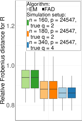
(a)

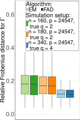
(b)

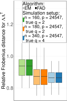
(c)

Figure S2: Relative Frobenius errors of FAD and EM for (a) correlation matrix $\mathbf{R}$, (b) signal matrix $\bm{\Gamma}$ and (c) $\bm{{\bm{\Lambda}}}\bm{{\bm{\Lambda}}}^{\top}$ on data-driven cases, with lighter ones for EM and darker ones for FAD.

Under the best fitted models, FAD and EM yields identical values of $\ell_{p}(\hat{{\bm{\Lambda}}},\hat{{\bm{\Psi}}}),$ $\hat{\bm{\Psi}},$ $\hat{\Gamma},$ and $\hat{\bm{\Lambda}}\hat{\bm{\Lambda}}^{\top}.$ Thus the relative errors (see Figure S2) in estimating these parameters are also identical.

III-C Additional experiments in high-noise scenarios

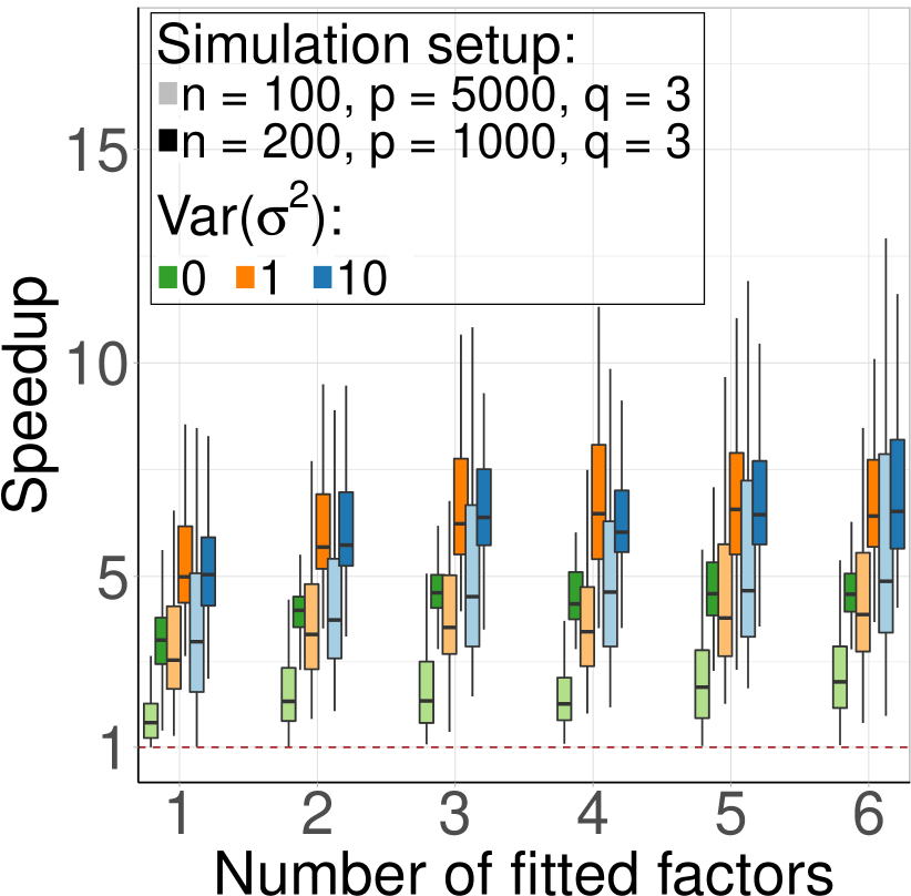
(a)

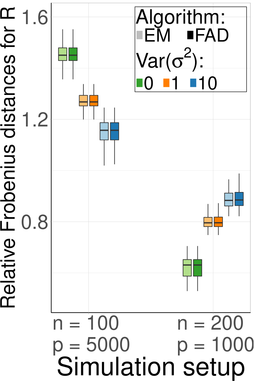
(b)

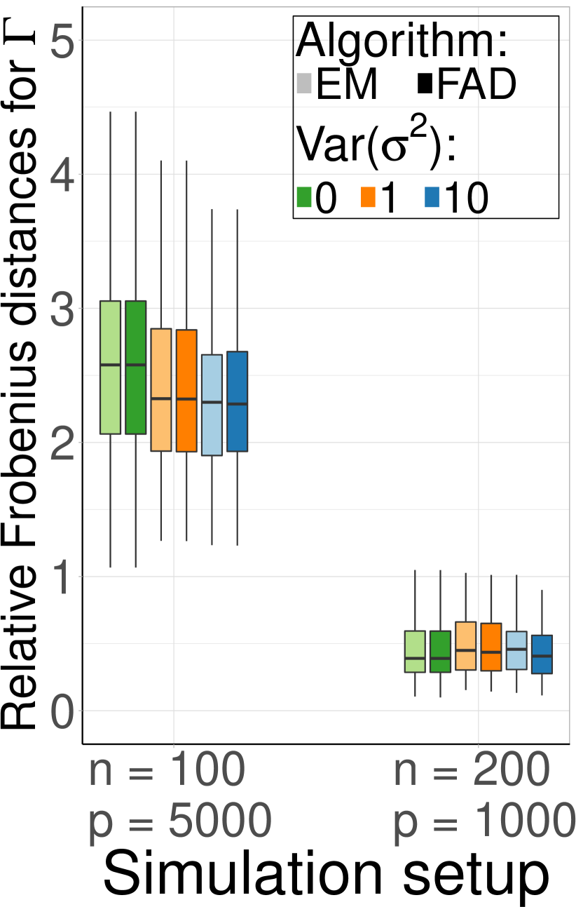
(c)

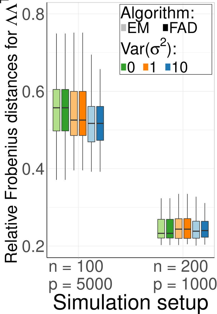
(d)

Figure S3: Relative speed of FAD to EM on dataset with high noise (a). Relative Frobenius errors of FAD and EM for (b) correlation matrix $\mathbf{R}$, (c) signal matrix $\bm{\Gamma}$ and (d) $\bm{{\bm{\Lambda}}}\bm{{\bm{\Lambda}}}^{\top}$.

We conclude this section by evaluating performance in situations where ostensibly, weak factors are hardly distinguished from high noise by SVD methods and where EM may be preferable [26]. We applied FAD and EM to the simulation setup of [26]: Here, the uniquenesses were sampled from three inverse Gamma distributions with unit means and variances of $0$, $1$ and $10$, and $(n,p)\in\{(200,1000),(100,5000)\}$. Figure S3 shows that our algorithm was substantially faster while having similar accuracy as EM.

IV Suicide ideation study

TABLE I: CPU times (rounded to the nearest seconds) for FAD and EM applied to the suicide ideation study dataset.

	$\bm{q}$	1	2	3	4	5	6	7	8	9	10
Attempters	FAD	3	3	4	5	5	6	6	7	9	9
	EM	146	173	207	198	229	236	228	250	239	254
Ideators	FAD	4	4	5	6	6	6	6	9	9	10
	EM	118	197	207	200	222	244	241	226	258	258
Controls	FAD	5	5	8	7	8	8	9	10	12	13
	EM	300	451	456	407	426	461	483	438	566	519

We applied EFA to data from [16] on an fMRI study conducted while 20 words connoting negative affects were shown to 9 suicide attempters, 8 suicide non-attempter ideators and 17 non-ideator control subjects. For each subject-word combination, [16] provided voxel-wise per cent changes in activation relative to the baseline in $50\!\times\!61\!\times\!23$ image volumes. Restricting attention to the 24547 in-brain voxels yields datasets for the attempters, ideators and controls of sizes $(n,p)\in\{(180,24547),(160,24547),(340,24547)\}$. We assumed each dataset to be a random sample from the multinormal distribution. Our interest was in determining if the variation in the per cent relative change in activation for each subject type can be explained by a few latent factors and whether there are differences in these factors between the three groups of subjects.

For each dataset, we performed EFA with $q=0,1,2,\ldots,10$ factors and using both FAD and EM. Table I demonstrates the computational benefits of using FAD over EM. We also used BIC to decide on the optimal $q$ ($q_{o}$) and obtained 2-factor models for both suicide attempters and ideators, and a 4-factor model for the control subjects. Figure 2 provides voxel-wise displays of the $q_{o}$ factor loadings, obtained using the quartimax criterion [27], for each type of subject. All the factor loadings are non-negligible only in voxels around the ventral attention network (VAN) which represents one of two sensory orienting systems that reorient attention towards notable stimuli and is closely related to involuntary actions [28]. However, there are differences between the factor loadings in each group and also among them.

Figure 2: Loading values of fitted factors for suicide attempters, ideators and controls.

For instance, for the suicide attempters, each factor is a contrast between different areas of the VAN, but the contrasts themselves differ between the two factors. The first factor for the ideators is a weighted mean of the voxels while the second factor is a contrast of the values at the VAN voxels. For the controls, the first three factors are different contrasts of the values at different voxels while the fourth factor is more or less a mean of the values at these voxels. Further, the factor loadings in the control group are more attenuated than for either the suicide attempters or ideators. While a detailed analysis of our results is outside the purview of this paper, we note that EFA has provided us with distinct factor loadings that potentially explains the variation in suicide attempters, non-attempter ideators and controls. However, our analysis assumed that the image volumes are independent and Gaussian: further approaches relaxing these assumptions may be appropriate.

V Discussion

In this paper, we propose a new ML-based EFA method called FAD using a sophisticated computational framework that achieves both high accuracy in parameter estimation and fast convergence via matrix-free algorithms. We implement a Lanczos method for computing partial singular values and vectors and a limited-memory quasi-Newton method for ML estimation. This implementation alleviates the computational limitations of current state-of-the-art algorithms and is capable of EFA for datasets with $p>>n$. In our experiments, FAD always converged but EM struggled with overfitted models. Although not demonstrated in this paper, FAD is also well-suited for distributed computing systems because it only uses the data matrix for computing matrix-vector products. FAD paves the way to develop fast methods for mixtures of factor analyzers and factor models for non-Gaussian data in high-dimensional clustering and classification problems.

S1 Supplementary materials for Methodology

S1.1 The EM algorithm for factor analysis on Gaussian data

The complete data log-likelihood function is

$$\begin{split}\ell_{C}(\bm{\mu},\bm{{\bm{\Lambda}}},\bm{{\bm{\Psi}}})=c&-\frac{n}{2}\log\det{\bm{\Psi}}-\frac{1}{2}\sum^{n}_{i=1}\{(\mathbf{Y}_{i}-\bm{\mu}-\bm{{\bm{\Lambda}}}\mathbf{Z}_{i})^{\top}{\bm{\Psi}}^{-1}(\mathbf{Y}_{i}-\bm{\mu}-\bm{{\bm{\Lambda}}}\mathbf{Z}_{i})\}\\ =c&-\frac{n}{2}\log\det{\bm{\Psi}}-\frac{1}{2}\mathrm{Tr}~{}\{\bm{{\bm{\Psi}}}^{-1}\sum^{n}_{i=1}{(\mathbf{Y}_{i}-\bm{\mu})(\mathbf{Y}_{i}-\bm{\mu})^{\top}}-2\bm{{\bm{\Psi}}}^{-1}\bm{{\bm{\Lambda}}}\sum^{n}_{i=1}{\mathbf{Z}_{i}}(\mathbf{Y}_{i}-\bm{\mu})^{\top}\}\\ &-\frac{1}{2}\mathrm{Tr}~{}\{\bm{{\bm{\Lambda}}}^{\top}\bm{{\bm{\Psi}}}^{-1}\bm{{\bm{\Lambda}}}\sum^{n}_{i=1}\mathbf{Z}_{i}\mathbf{Z}_{i}^{\top}\},\end{split}$$ (S1)

where $c$ is a constant that does not depend on the parameters.

S1.11 E-Step computations

Since the ML estimate of $\bm{\mu}$ is $\bar{\mathbf{Y}}$, at the current estimates $\bm{{\bm{\Lambda}}}_{t}$ and $\bm{{\bm{\Psi}}}_{t}$ , the expected complete log-likelihood or so called $\mathrm{Q}$ function is given by

$$\begin{split}\mathrm{Q}(\bm{{\bm{\Lambda}}}_{t+1},\bm{{\bm{\Psi}}}_{t+1}|\bar{\mathbf{Y}},\bm{{\bm{\Lambda}}}_{t},\bm{{\bm{\Psi}}}_{t})=&\mathrm{E}[\ell_{C}(\bm{{\bm{\Lambda}}},\bm{{\bm{\Psi}}}|\mathbf{Y},\bm{{\bm{\Lambda}}}_{t},\bm{{\bm{\Psi}}}_{t}]\\ =&-\frac{n}{2}\log\det{\bm{\Psi}}-\frac{n}{2}\mathrm{Tr}~{}\bm{{\bm{\Psi}}}^{-1}\mathbf{S}-\mathrm{Tr}~{}\{\bm{{\bm{\Psi}}}^{-1}\bm{{\bm{\Lambda}}}\sum^{n}_{i=1}{\mathrm{E}[\mathbf{Z}_{i}|\mathbf{Y},\bm{{\bm{\Lambda}}}_{t},\bm{{\bm{\Psi}}}_{t}]}(\mathbf{Y}_{i}-\bar{\mathbf{Y}})^{\top}\}\\ &+\frac{1}{2}\mathrm{Tr}~{}\{\bm{{\bm{\Lambda}}}^{\top}\bm{{\bm{\Psi}}}^{-1}\bm{{\bm{\Lambda}}}\frac{1}{n}\sum^{n}_{i=1}\mathrm{E}[\mathbf{Z}_{i}\mathbf{Z}_{i}^{\top}|\mathbf{Y},\bm{{\bm{\Lambda}}}_{t},\bm{{\bm{\Psi}}}_{t}]\}.\end{split}$$ (S2)

Since $\mathbf{Z}_{i}|\mathbf{Y},\bm{{\bm{\Lambda}}}_{t},\bm{{\bm{\Psi}}}_{t}\sim\mathcal{N}_{q}(\bm{{\bm{\Lambda}}}_{t}^{\top}\mathbf{{\bm{\Sigma}}}_{t}^{-1}(\mathbf{Y}_{i}-\bar{\mathbf{Y}}),(\mathbf{I}_{q}+\bm{{\bm{\Lambda}}}_{t}^{\top}\bm{{\bm{\Psi}}}_{t}^{-1}\bm{{\bm{\Lambda}}}_{t})^{-1})$. Then,

$$\begin{split}&\mathrm{E}[\mathbf{Z}_{i}|\mathbf{Y},\bm{{\bm{\Lambda}}}_{t},\bm{{\bm{\Psi}}}_{t}]=\bm{{\bm{\Lambda}}}_{t}^{\top}\mathbf{{\bm{\Sigma}}}_{t}^{-1}(\mathbf{Y}_{i}-\bar{\mathbf{Y}})\\ \end{split}$$ (S3)

and

$$\begin{split}\mathrm{E}[\mathbf{Z}_{i}\mathbf{Z}_{i}^{\top}|\mathbf{Y},\bm{{\bm{\Lambda}}}_{t},\bm{{\bm{\Psi}}}_{t}]=&\mathrm{Var}[\mathbf{Z}_{i}|\mathbf{Y},\bm{{\bm{\Lambda}}}_{t},\bm{{\bm{\Psi}}}_{t}]+\mathrm{E}[\mathbf{Z}_{i}|\mathbf{Y},\bm{{\bm{\Lambda}}}_{t},\bm{{\bm{\Psi}}}_{t}]\mathrm{E}[\mathbf{Z}_{i}^{\top}|\mathbf{Y}_{i},\bar{\mathbf{Y}},\bm{{\bm{\Lambda}}}_{t},\bm{{\bm{\Psi}}}_{t}]\\ =&(\mathbf{I}_{q}+\bm{{\bm{\Lambda}}}_{t}^{\top}\bm{{\bm{\Psi}}}_{t}^{-1}\bm{{\bm{\Lambda}}}_{t})^{-1}+\bm{{\bm{\Lambda}}}_{t}^{\top}\mathbf{{\bm{\Sigma}}}_{t}^{-1}(\mathbf{Y}_{i}-\bar{\mathbf{Y}})(\mathbf{Y}_{i}-\bar{\mathbf{Y}})^{\top}\mathbf{{\bm{\Sigma}}}_{t}^{-1}\bm{{\bm{\Lambda}}}_{t}.\end{split}$$ (S4)

S1.12 M-Step computations

The parameters $\bm{{\bm{\Lambda}}}_{t+1}$ and $\bm{{\bm{\Psi}}}_{t+1}$ are obtained by maximizing $\mathrm{Q}(\bm{{\bm{\Lambda}}}_{t+1},\bm{{\bm{\Psi}}}_{t+1}|\bar{\mathbf{Y}},\bm{{\bm{\Lambda}}}_{t},\bm{{\bm{\Psi}}}_{t})$ following equation S2. Specifically, given ${\mathbf{Y}}$, $\bm{{\bm{\Lambda}}}_{t}$ and $\bm{{\bm{\Psi}}}_{t}$, the maximizer $\bm{{\bm{\Lambda}}}_{t+1}$ is given by

$$\begin{split}\hat{\bm{{\bm{\Lambda}}}}_{t+1}=&(\frac{1}{n}\sum^{n}_{i=1}(\mathbf{Y}_{i}-\bar{\mathbf{Y}}){\mathrm{E}[\mathbf{Z}_{i}^{\top}|\mathbf{Y},\bm{{\bm{\Lambda}}}_{t},\bm{{\bm{\Psi}}}_{t}]})(\frac{1}{n}\sum^{n}_{i=1}{\mathrm{E}[\mathbf{Z}_{i}\mathbf{Z}_{i}^{\top}|\mathbf{Y},\bm{{\bm{\Lambda}}}_{t},\bm{{\bm{\Psi}}}_{t}]})^{-1}\\ =&\mathbf{S}\mathbf{{\bm{\Sigma}}}^{-1}_{t}\bm{{\bm{\Lambda}}}_{t}((\mathbf{I}_{q}+\bm{{\bm{\Lambda}}}^{\top}_{t}\bm{{\bm{\Psi}}}^{-1}_{t}\bm{{\bm{\Lambda}}}_{t})^{-1}+\bm{{\bm{\Lambda}}}^{\top}_{t}\mathbf{{\bm{\Sigma}}}^{-1}_{t}\mathbf{S}\mathbf{{\bm{\Sigma}}}^{-1}_{t}\bm{{\bm{\Lambda}}}_{t})^{-1}\\ \end{split}$$ (S5)

where $\mathbf{{\bm{\Sigma}}}_{t}=\bm{{\bm{\Lambda}}}_{t}\bm{{\bm{\Lambda}}}^{\top}_{t}+\bm{{\bm{\Psi}}}_{t}$. By Woodbury matrix identity [29], $\mathbf{{\bm{\Sigma}}}^{-1}_{t}\bm{{\bm{\Lambda}}}_{t}=\bm{{\bm{\Psi}}}^{-1}_{t}\bm{{\bm{\Lambda}}}_{t}(\mathbf{I}_{q}+\bm{{\bm{\Lambda}}}^{\top}_{t}\bm{{\bm{\Psi}}}^{-1}_{t}\bm{{\bm{\Lambda}}}_{t})^{-1}$, so S5 can be simplified as

$$\begin{split}\hat{\bm{{\bm{\Lambda}}}}_{t+1}=&\mathbf{S}\bm{{\bm{\Psi}}}^{-1}_{t}\bm{{\bm{\Lambda}}}_{t}(\mathbf{I}_{q}+\bm{{\bm{\Lambda}}}^{\top}_{t}\bm{{\bm{\Psi}}}^{-1}_{t}\bm{{\bm{\Lambda}}}_{t})^{-1}((\mathbf{I}_{q}+\bm{{\bm{\Lambda}}}^{\top}_{t}\bm{{\bm{\Psi}}}^{-1}_{t}\bm{{\bm{\Lambda}}}_{t})^{-1}+\bm{{\bm{\Lambda}}}^{\top}_{t}\mathbf{{\bm{\Sigma}}}^{-1}_{t}\mathbf{S}\bm{{\bm{\Psi}}}^{-1}_{t}\bm{{\bm{\Lambda}}}_{t}(\mathbf{I}_{q}+\bm{{\bm{\Lambda}}}^{\top}_{t}\bm{{\bm{\Psi}}}^{-1}_{t}\bm{{\bm{\Lambda}}}_{t})^{-1})^{-1}\\ =&\mathbf{S}\bm{{\bm{\Psi}}}^{-1}_{t}\bm{{\bm{\Lambda}}}_{t}(\mathbf{I}_{q}+\bm{{\bm{\Lambda}}}^{\top}_{t}\mathbf{{\bm{\Sigma}}}^{-1}_{t}\mathbf{S}\bm{{\bm{\Psi}}}^{-1}_{t}\bm{{\bm{\Lambda}}}_{t})^{-1}.\end{split}$$ (S6)

Next, given $\mathbf{Y},$ $\bm{{\bm{\Lambda}}}_{t}$, $\bm{{\bm{\Psi}}}_{t}$ and $\hat{\bm{{\bm{\Lambda}}}}_{t+1}$, the ML estimate of $\bm{{\bm{\Psi}}}_{t+1}$ is given by

$$\begin{split}\hat{\bm{{\bm{\Psi}}}}_{t+1}=\mathrm{diag}\Big{(}&\mathbf{S}-\frac{2}{n}\sum^{n}_{i=1}(\mathbf{Y}_{i}-\bar{\mathbf{Y}}){\mathrm{E}[\mathbf{Z}_{i}^{\top}|\mathbf{Y},\bm{{\bm{\Lambda}}}_{t},\bm{{\bm{\Psi}}}_{t}]}\hat{\bm{{\bm{\Lambda}}}}^{\top}_{t+1}\\ &+\hat{\bm{{\bm{\Lambda}}}}_{t+1}\frac{1}{n}\sum^{n}_{i=1}{\mathrm{E}[\mathbf{Z}_{i}\mathbf{Z}_{i}^{\top}|\mathbf{Y},\bm{{\bm{\Lambda}}}_{t},\bm{{\bm{\Psi}}}_{t}]})^{-1}\hat{\bm{{\bm{\Lambda}}}}^{\top}_{t+1}\Big{)}.\end{split}$$ (S7)

Substitute with S5, we get

$$\begin{split}\hat{\bm{{\bm{\Psi}}}}_{t+1}=&\mathrm{diag}\Big{(}\mathbf{S}-\frac{2}{n}\sum^{n}_{i=1}(\mathbf{Y}_{i}-\bar{\mathbf{Y}}){\mathrm{E}[\mathbf{Z}_{i}^{\top}|\mathbf{Y},\bm{{\bm{\Lambda}}}_{t},\bm{{\bm{\Psi}}}_{t}]}\hat{\bm{{\bm{\Lambda}}}}^{\top}_{t+1}\\ &\qquad\ +\frac{1}{n}\sum^{n}_{i=1}(\mathbf{Y}_{i}-\bar{\mathbf{Y}}){\mathrm{E}[\mathbf{Z}_{i}^{\top}|\mathbf{Y},\bm{{\bm{\Lambda}}}_{t},\bm{{\bm{\Psi}}}_{t}]}\hat{\bm{{\bm{\Lambda}}}}^{\top}_{t+1}\Big{)}\\ =&\mathrm{diag}\Big{(}\mathbf{S}-2\mathbf{S}\mathbf{{\bm{\Sigma}}}^{-1}_{t}\bm{{\bm{\Lambda}}}_{t}\hat{\bm{{\bm{\Lambda}}}}^{\top}_{t+1}\Big{)}.\end{split}$$ (S8)

S1.2 Proof of Lemma 1

From equation 1, the ML estimates of $\bm{{\bm{\Lambda}}}$ and $\bm{{\bm{\Psi}}}$ are obtained by solving the score equations

$$\begin{split}\begin{cases}&\bm{{\bm{\Lambda}}}(\mathbf{I}_{q}+\bm{{\bm{\Lambda}}}^{\top}\bm{{\bm{\Psi}}}^{-1}\bm{{\bm{\Lambda}}})=\mathbf{S}\bm{{\bm{\Psi}}}^{-1}\bm{{\bm{\Lambda}}}\\ &\bm{{\bm{\Psi}}}=\mathrm{diag}(\mathbf{S}-\bm{{\bm{\Lambda}}}\bm{{\bm{\Lambda}}}^{\top})\end{cases}\end{split}$$ (S9)

From $\bm{{\bm{\Lambda}}}(\mathbf{I}_{q}+\bm{{\bm{\Lambda}}}^{\top}\bm{{\bm{\Psi}}}^{-1}\bm{{\bm{\Lambda}}})=\mathbf{S}\bm{{\bm{\Psi}}}^{-1}\bm{{\bm{\Lambda}}}$, we have

$$\bm{{\bm{\Psi}}}^{-1/2}\bm{{\bm{\Lambda}}}(\mathbf{I}_{q}+(\bm{{\bm{\Psi}}}^{-1/2}\bm{{\bm{\Lambda}}})^{\top}\bm{{\bm{\Psi}}}^{-1/2}\bm{{\bm{\Lambda}}})=\bm{{\bm{\Psi}}}^{-1/2}\mathbf{S}\bm{{\bm{\Psi}}}^{-1/2}\bm{{\bm{\Psi}}}^{-1/2}\bm{{\bm{\Lambda}}}.$$ (S10)

Suppose that $\bm{{\bm{\Psi}}}^{-1/2}\mathbf{S}\bm{{\bm{\Psi}}}^{-1/2}=\mathbf{V}\mathbf{D}\mathbf{V}^{\top}$ and that the diagonal elements in $\mathbf{D}$ are in decreasing order with $\theta_{1}\geq\theta_{2}\geq,\cdots,\geq\theta_{p}$. Let $\mathbf{D}=\begin{bmatrix}\mathbf{D}_{q}&0\\ 0&\mathbf{D}_{m}\end{bmatrix}$ with $m=p-q$ and $\mathbf{D}_{q}$ containing the largest $q$ eigenvalues $\theta_{1}\geq\theta_{2}\geq,\cdots,\geq\theta_{q}$. The corresponding $q$ eigenvectors forms columns of matrix $\mathbf{V}_{q}$ so that $\mathbf{V}=[\mathbf{V}_{q},\mathbf{V}_{m}]$. Then, if $\mathbf{D}_{q}>\mathbf{I}_{q}$, S10 shows that

$$\bm{{\bm{\Lambda}}}=\bm{{\bm{\Psi}}}^{1/2}\mathbf{V}_{q}(\mathbf{D}_{q}-\mathbf{I}_{q})^{1/2}.$$ (S11)

The square roots of $\theta_{1},\cdots,\theta_{q}$ are the $q$ largest singular values of $n^{-1/2}(\mathbf{Y}-\mathbf{1}\bar{\mathbf{Y}}^{\top})\bm{{\bm{\Psi}}}^{-1/2}$ and columns in $\mathbf{V}_{q}$ are then the corresponding $q$ right-singular vectors. Hence, conditional on $\bm{{\bm{\Psi}}}$, $\bm{{\bm{\Lambda}}}$ is maximized at $\hat{\bm{{\bm{\Lambda}}}}=\bm{{\bm{\Psi}}}^{1/2}\mathbf{V}_{q}\bm{\Delta}$, where $\bm{\Delta}$ is a diagonal matrix with elements $\mathrm{max}(\theta_{i}-1,0)^{1/2},i=1,\cdots,q$.

From the construction of $\mathbf{V}_{q}$ and $\mathbf{V}_{m}$, we have $\mathbf{V}^{\top}_{q}\mathbf{V}_{q}=\mathbf{I}_{q}\text{, }\mathbf{V}^{\top}_{m}\mathbf{V}_{m}=\mathbf{I}_{m}\text{, }\mathbf{V}_{q}\mathbf{V}^{\top}_{q}+\mathbf{V}_{m}\mathbf{V}^{\top}_{m}=\mathbf{I}_{p}\text{, }\mathbf{V}^{\top}_{q}\mathbf{V}_{m}=\bm{0}$ and hence, $(\mathbf{V}_{q}\mathbf{D}_{q}\mathbf{V}^{\top}_{q}+\mathbf{V}_{m}\mathbf{V}^{\top}_{m})(\mathbf{V}_{q}\mathbf{D}^{-1}_{q}\mathbf{V}^{\top}_{q}+\mathbf{V}_{m}\mathbf{V}^{\top}_{m})=\mathbf{I}_{p}$.

Let $\mathbf{A}=\mathbf{V}_{q}\bm{\Delta}^{2}\mathbf{V}^{\top}_{q}$. Then $\mathbf{A}\mathbf{A}=\mathbf{V}_{q}\bm{\Delta}^{4}\mathbf{V}^{\top}_{q}$ and

$$\begin{split}|\mathbf{A}+\mathbf{I}_{p}|=&|(\mathbf{A}+\mathbf{I}_{p})\mathbf{A}|/|\mathbf{A}|\\ =&|\mathbf{V}_{q}(\bm{\Delta}^{4}+\bm{\Delta}^{2})\mathbf{V}^{\top}_{q}|/|\mathbf{V}_{q}\bm{\Delta}^{2}\mathbf{V}^{\top}_{q}|\\ =&|\bm{\Delta}^{2}+\mathbf{I}_{q}|=\prod_{j=1}^{q}{\theta_{j}}\end{split}$$ (S12)

and

$$\begin{split}(\mathbf{A}+\mathbf{I}_{p})^{-1}=&(\mathbf{V}_{q}\bm{\Delta}^{2}\mathbf{V}^{\top}_{q}+\mathbf{V}_{q}\mathbf{V}^{\top}_{q}+\mathbf{V}_{m}\mathbf{V}^{\top}_{m})^{-1}\\ =&(\mathbf{V}_{q}(\bm{\Delta}^{2}+\mathbf{I}_{q})\mathbf{V}^{\top}_{q}+\mathbf{V}_{m}\mathbf{V}^{\top}_{m})^{-1}\\ =&(\mathbf{V}_{q}\mathbf{D}_{q}\mathbf{V}^{\top}_{q}+\mathbf{V}_{m}\mathbf{V}^{\top}_{m})^{-1}\\ =&\mathbf{V}_{q}\mathbf{D}^{-1}_{q}\mathbf{V}^{\top}_{q}+\mathbf{V}_{m}\mathbf{V}^{\top}_{m}.\end{split}$$ (S13)

Based on S12 and S13 and equation 2, the profile log-likelihood is given by

$$\begin{split}\ell_{p}(\bm{{\bm{\Psi}}})=c&-\frac{n}{2}\log{|\hat{\bm{{\bm{\Lambda}}}}\hat{\bm{{\bm{\Lambda}}}}^{\top}+\bm{{\bm{\Psi}}}|}-\frac{n}{2}\mathrm{Tr}~{}(\hat{\bm{{\bm{\Lambda}}}}\hat{\bm{{\bm{\Lambda}}}}^{\top}+\bm{{\bm{\Psi}}})^{-1}\mathbf{S}\\ =c&-\frac{n}{2}\Big{\{}\log|\bm{{\bm{\Psi}}}^{1/2}(\mathbf{V}_{q}\bm{\Delta}^{2}\mathbf{V}^{\top}_{q}+\mathbf{I}_{p})\bm{{\bm{\Psi}}}^{1/2}|+\mathrm{Tr}~{}\bm{{\bm{\Psi}}}^{1/2}(\mathbf{V}_{q}\bm{\Delta}^{2}\mathbf{V}^{\top}_{q}+\mathbf{I}_{p})\bm{{\bm{\Psi}}}^{1/2})^{-1}\mathbf{S}\Big{\}}\\ =c&-\frac{n}{2}\Big{\{}\log\det{\bm{\Psi}}+\log{|\mathbf{V}_{q}\bm{\Delta}^{2}\mathbf{V}^{\top}_{q}+\mathbf{I}_{p}|}+\mathrm{Tr}~{}(\mathbf{V}_{q}\mathbf{D}^{-1}_{q}\mathbf{V}^{\top}_{q}+\mathbf{V}_{m}\mathbf{V}^{\top}_{m})\bm{{\bm{\Psi}}}^{-1/2}\mathbf{S}\bm{{\bm{\Psi}}}^{-1/2}\Big{\}}\\ =c&-\frac{n}{2}\Big{\{}\log\det{\bm{\Psi}}+\sum_{j=1}^{q}{\log{\theta_{j}}}+\mathrm{Tr}~{}(\mathbf{D}^{-1}_{q}\mathbf{V}^{\top}_{q}\mathbf{V}\mathbf{D}\mathbf{V}^{\top}\mathbf{V}_{q}+\mathrm{Tr}~{}\mathbf{V}^{\top}_{m}\mathbf{V}\mathbf{D}\mathbf{V}^{\top}\mathbf{V}_{m}\Big{\}}\\ =c&-\frac{n}{2}\Big{\{}\log\det{\bm{\Psi}}+\sum_{j=1}^{q}{\log{\theta_{j}}}+\mathrm{Tr}~{}\mathbf{D}^{-1}_{q}\mathbf{D}_{q}+\mathrm{Tr}~{}\mathbf{D}_{m}\Big{\}}\\ =c&-\frac{n}{2}\Big{\{}\log\det{\bm{\Psi}}+\sum_{j=1}^{q}{\log{\theta_{j}}}+q+\mathrm{Tr}~{}\bm{{\bm{\Psi}}}^{-1}\mathbf{S}-\sum_{j=1}^{q}{\theta_{j}}\Big{\}}.\end{split}$$ (S14)

S2 Additional results for simulation studies

S2.1 Average CPU time

TABLE S1: Average CPU time (in seconds) of FAD and EM applied with 1-6 factors for randomly simulated datasets where true $q=3$.

		1	2	3	4	5	6
$(n,p,q)=(10^{2},10^{3},3)$	FAD	0.101	0.092	0.096	0.116	0.122	0.128
	EM	2.494	2.519	3.076	2.012	2.075	2.162
$(n,p,q)=(15^{2},15^{3},3)$	FAD	0.639	0.514	0.486	0.841	0.966	1.025
	EM	24.798	22.885	27.906	16.822	16.630	15.722
$(n,p,q)=(20^{2},20^{3},3)$	FAD	2.933	2.658	2.580	7.135	7.863	8.590
	EM	57.052	57.527	81.463	49.689	48.508	49.504

TABLE S2: Average CPU time (in seconds) of FAD and EM applied with 1-10 factors for randomly simulated datasets where true $q=5$.

		1	2	3	4	5	6	7	8	9	10
$(n,p,q)=(10^{2},10^{3},5)$	FAD	0.102	0.095	0.096	0.096	0.094	0.119	0.124	0.128	0.134	0.137
	EM	2.290	2.539	2.808	2.800	2.985	2.301	2.327	2.097	2.166	2.196
$(n,p,q)=(15^{2},15^{3},5)$	FAD	0.667	0.513	0.501	0.507	0.497	0.828	0.919	1.039	1.108	1.143
	EM	22.545	21.066	22.300	22.197	26.300	16.544	15.796	14.767	14.292	14.789
$(n,p,q)=(20^{2},20^{3},5)$	FAD	2.937	2.687	2.553	2.583	2.590	7.114	8.167	9.238	10.426	11.157
	EM	47.200	47.333	49.867	49.956	71.308	47.469	47.119	43.828	45.304	44.141

TABLE S3: Average CPU time (in seconds) of FAD and EM applied for data-driven models.

		1	2	3	4	5	6	7	8
$(n,p,q)=(160,24547,2)$	FAD	5.007	4.222	10.835	13.636	–	–	–	–
	EM	253.021	304.909	311.916	303.712	–	–	–	–
$(n,p,q)=(180,24547,2)$	FAD	4.927	4.104	10.411	12.058	–	–	–	–
	EM	287.824	345.504	331.919	314.723	–	–	–	–
$(n,p,q)=(340,24547,4)$	FAD	6.645	7.121	7.449	6.688	22.294	26.575	31.109	34.208
	EM	648.759	734.226	745.902	735.263	767.010	789.614	802.502	748.395

S2.2 Estimation errors in parameters

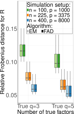
(a)

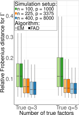
(b)

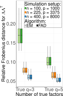
(c)

Figure S1: Relative Frobenius errors of FAD and EM for (a) correlation matrix $\mathbf{R}$, (b) signal matrix $\bm{\Gamma}$ and (c) $\bm{{\bm{\Lambda}}}\bm{{\bm{\Lambda}}}^{\top}$ on randomly simulated cases, with lighter ones for EM and darker ones for FAD.

S2.3 Performance of FAD compared to EM for high-noise models

References

- [1] T. W. Anderson, An Introduction to Multivariate Statistical Analysis, ser. Wiley Series in Probability and Statistics. Wiley, 2003. [Online]. Available: https://books.google.com/books?id=Cmm9QgAACAAJ
- [2] D. N. Lawley, “The estimation of factor loadings by the method of maximum likelihood,” Proceedings of the Royal Society of Edinburgh, vol. 60, pp. 64–82, 01 1940.
- [3] K. G. Jöreskog, “Some contributions to maximum likelihood factor analysis,” Psychometrika, vol. 32, pp. 443–482, 12 1967.
- [4] D. N. Lawley and A. E. Maxwell, “Factor analysis as a statistical method,” Journal of the Royal Statistical Society. Series D (The Statistician), vol. 12, pp. 209–229, 1962.
- [5] K. V. Mardia, J. T. Kent, and J. M. Bibby, Multivariate analysis. Elsevier Amsterdam, 2006.
- [6] R. Sundberg and U. Feldmann, “Exploratory factor analysis–parameter estimation and scores prediction with high-dimensional data,” Journal of Multivariate Analysis, vol. 148, pp. 49–59, 2016.
- [7] J. T. Leek and J. D. Storey, “Capturing heterogeneity in gene expression studies by surrogate variable analysis,” PLoS Genetics, vol. 3, no. 9, p. e161, 2007.
- [8] J. T. Leek, “Svaseq: Removing batch effects and other unwanted noise from sequencing data,” Nucleic Acids Research, vol. 42, no. 21, p. e161, 2014.
- [9] F. Buettner, N. Pratanwanich, D. J. McCarthy, J. C. Marioni, and O. Stegle, “f-sclvm: Scalable and versatile factor analysis for single-cell rna-seq,” Genome biology, vol. 18, no. 1, p. 212, 2017.
- [10] I. Pournara and L. Wernisch, “Factor analysis for gene regulatory networks and transcription factor activity profiles,” BMC Bioinformatics, vol. 8, p. 61, 02 2007.
- [11] C. T. Ng, C. Y. Yau, and N. H. Chan, “Likelihood inferences for high-dimensional factor analysis of time series with applications in finance,” Journal of Computational and Graphical Statistics, vol. 24, pp. 866–884, 11 2014.
- [12] N. T. Trendafilov and S. Unkel, “Exploratory factor analysis of data matrices with more variables than observations,” Journal of Computational and Graphical Statistics, vol. 20, no. 4, pp. 874–891, 2011.
- [13] D. Robertson and J. Symons, “Maximum likelihood factor analysis with rank-deficient sample covariance matrices,” Journal of Multivariate Analysis, vol. 98, no. 4, pp. 813–828, 2007.
- [14] D. B. Rubin and D. T. Thayer, “Em algorithms for ml factor analysis,” Psychometrika, vol. 47, pp. 69–76, 02 1982.
- [15] R Core Team, R: A Language and Environment for Statistical Computing, R Foundation for Statistical Computing, Vienna, Austria, 2019. [Online]. Available: https://www.R-project.org/
- [16] M. A. Just, L. A. Pan, V. L. Cherkassky, D. L. McMakin, C. B. Cha, M. K. Nock, and D. P. Brent, “Machine learning of neural representations of suicide and emotion concepts identifies suicidal youth,” Nature Human Behaviour, vol. 1, pp. 911–919, 2017.
- [17] G. McLachlan and T. Krishnan, The EM Algorithm and Extensions, ser. Wiley Series in Probability and Statistics. Wiley, 1996. [Online]. Available: https://books.google.com/books?id=iRSWQgAACAAJ
- [18] C. Liu and D. B. Rubin, “Maximum likelihood estimation of factor analysis using the ecme algorithm with complete and incomplete data,” Statistica Sinica, vol. 8, pp. 729–747, 08 2002.
- [19] R. Varadhan and C. Roland, “Simple and globally convergent methods for accelerating the convergence of any em algorithm,” Scandinavian Journal of Statistics, vol. 35, pp. 335–353, 06 2008.
- [20] J. Baglama and L. Reichel, “Augmented implicitly restarted lanczos bidiagonalization methods,” SIAM Journal on Scientific Computing, vol. 27, no. 1, pp. 19–42, 2005.
- [21] S. Dutta and D. Mondal, “An h-likelihood method for spatial mixed linear model based on intrinsic autoregressions,” Journal of the Royal Statistical Society: Series B (Statistical Methodology), vol. 77, pp. 699–726, 09 2014.
- [22] J. H. Wilkinson, “The calculation of the eigenvectors of codiagonal matrices,” Computer Journal, vol. 1, pp. 90–96, 02 1958.
- [23] R. H. Byrd, J. N. P. Lu, and C. Zhu, “A limited memory algorithm for bound constrained optimization,” SIAM Journal on Scientific Computing, vol. 16, pp. 1190–1208, 1995.
- [24] C. Zhu, R. H. Byrd, P. Lu, and J. Nocedal, “Algorithm 778: L-bfgs-b: Fortran subroutines for large-scale bound-constrained optimization,” ACM Transactions on Mathematical Software, vol. 23, pp. 550–560, 1994.
- [25] G. E. Schwarz, “Estimating the dimension of a model,” The Annals of Statistics, vol. 6, pp. 461–464, 03 1978.
- [26] A. B. Owen and J. Wang, “Bi-cross-validation for factor analysis,” Statistical Science, vol. 31, pp. 119–139, 03 2015.
- [27] A. B. Costello and J. Osborne, “Best practices in exploratory factor analysis: Four recommendations for getting the most from your analysis,” Practical Assessment, Research & Evaluation, vol. 10, pp. 1–9, 01 2005.
- [28] S. Vossel, J. J. Geng, and G. R. Fink, “Dorsal and ventral attention systems: Distinct neural circuits but collaborative roles,” The Neuroscientist, vol. 20, no. 2, pp. 150–159, 2014.
- [29] H. V. Henderson and S. R. Searle, “On deriving the inverse of a sum of matrices,” SIAM Review, vol. 23, no. 1, pp. 53–60, 1981.