Semantic Guided Single Image Reflection Removal

Abstract.

Reflection is common when we see through a glass window, which not only is a visual disturbance but also influences the performance of computer vision algorithms. Removing the reflection from a single image, however, is highly ill-posed since the color at each pixel needs to be separated into two values belonging to the clear background and the reflection respectively. To solve this, existing methods use additional priors such as reflection layer smoothness, double reflection effect, and color consistency to distinguish the two layers. However, these low-level priors may not be consistently valid in real cases. In this paper, inspired by the fact that human beings can separate the two layers easily by recognizing the objects and understanding the scene, we propose to use the object semantic cue, which is high-level information, as the guidance to help reflection removal. Based on the data analysis, we develop a multi-task end-to-end deep learning method with a semantic guidance component, to solve reflection removal and semantic segmentation jointly. Extensive experiments on different datasets show significant performance gain when using high-level object-oriented information. We also demonstrate the application of our method to other computer vision tasks.

1. Introduction

When taking a photo of objects behind the glass window, unwanted reflection frequently appears, which not only is visually disturbing but may also affect the performance of other computer vision algorithms (e.g., classification (Liu et al., 2020b), object detection (Redmon and Farhadi, 2018), scene parsing (Zhou et al., 2017), etc.). To solve this problem, reflection removal has been explored by a number of existing works (Fan et al., 2017; Li and Brown, 2013; Nandoriya et al., 2017; Wei et al., 2019; Wen et al., 2019; Wieschollek et al., 2018). Single image reflection removal is a challenging problem, i.e., it only takes one single image as the input and aims to separate it into two outputs, the clear background and the reflection. More formally, given an input image with reflection, denoted as $\mathbf{I}$, we need to separate it into background $\mathbf{B}$ and reflection $\mathbf{R}$ (Li and Brown, 2014; Zhang et al., 2018):

(1) $$\mathbf{I}=\mathbf{B}+\mathbf{R}.$$

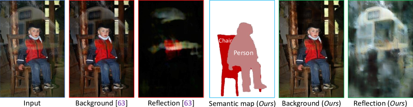
Figure 1. From left to right: The input, background estimation, and reflection estimation from one of the state-of-the-art methods (Zhang et al., 2018). Our semantic segmentation, background estimation, and reflection estimation. Our approach performs a joint task of reflection removal and semantic segmentation. Understanding the semantics of the background, our methods can provide much clearer separation results.

Apparently, Eqn. (1) is ill-posed due to there are two unknowns (B and R) to be divided from only one known (I). Without any constraints, there are numerously possible solutions. Earlier methods propose different priors as constraints (e.g., relative smoothness (Li and Brown, 2014), chromaticity consistency (Zhao et al., 2015), ghost effect (Shih et al., 2015), etc.) to get a meaningful solution. However, such low-level priors are not general enough in real cases. Fan et al. (Fan et al., 2017) are the first to train a deep neural network for this task with losses on colors and edges. Following (Fan et al., 2017), other methods have been proposed in the direction of new network design (Wan et al., 2017, 2018; Wei et al., 2019; Wen et al., 2019; Yang et al., 2018; Zhang et al., 2018), new loss functions like perceptual loss (Zhang et al., 2018) and GAN loss (Wen et al., 2019; Ma et al., 2019), or attention modules (Wei et al., 2019). All of them use a network to learn a mapping from a blended reflection image to a clear background. While adversarial learning using GAN loss and contextual attention may provide information beyond low-level features, the object-level semantic information has never been explored. We have observed that using only the low-level information (even equips with adversarial learning) is insufficient for the reflection separation due to the high ambiguity in low-level appearance.

Fig. 1 shows a case, though (Zhang et al., 2018) introduced high-level constraints, they still cannot handle this case well. In this paper, we use a simple intuition from human cognition, which we humans can easily separate the mixed visual appearance into reflection and background layers by object level priors. One can first recognize the internal objects and quickly assign them to the background layer. Take Fig. 1 as an example, we understand that the background is a person sitting on a chair so that all human parts and the chair need to be in the background layer. This enables us to recover the background correctly and meanwhile recover the reflection layer clearly.

However, implementing such an idea is not trivial, because it is not guaranteed to get the robust semantics from the input image with reflection, while a cleaner image is of many benefits to the estimation of semantic segmentation. To enable this, we assume the intensity of the background image is stronger than the reflection, which is the same as all existing reflection removal methods. Therefore, the background’s semantics is more significant than that in the reflection layer in this situation. We then propose a novel multi-task learning method for single image reflection removal, named Semantic Guided Reflection Removal Network (SGR²N). This means the semantic estimation and reflection removal are learned and optimized simultaneously. Furthermore, we design the semantic guidance block, which explicitly utilizes the semantic to guide the reflection removal.

To evaluate the effectiveness of SGR²N, we conducted systematical experiments on three datasets. Experiments report consistent and significant performance improvement on all three datasets. Ablation study and analytical experiments also show the effectiveness of our method.

Contributions. We summary the contributions as follows:

• To the best of our knowledge, it is the first method to use pixel-level semantic information as guidance for reflection removal, which is an explicit way to represent and use semantic information. And our method jointly solves the semantic segmentation and reflection removal from a single image.

• We propose a novel multi-task and end-to-end network with a novel semantic guidance block to achieve single simultaneous image reflection removal (main-task) and semantic analysis (sub-task).

• We demonstrate the effectiveness of the method through comprehensive experiments on both three datasets.

2. Related Work

Multiple-input methods. Many works solve Eqn. (1) with multiple inputs. Methods (Sinha et al., 2012; Guo et al., 2014; Li and Brown, 2013; Simon and Park, 2015; Nandoriya et al., 2017) assume the reflection and background layer are at different depth planes which can be separated by multi-view depth estimation. To align multiple inputs, optical flow is adopted to achieve reflection removal (Xue et al., 2015; Yang et al., 2016; Liu et al., 2020a). Another group of work uses a pair of with/without flash points to make reflection removal like (Agrawal et al., 2005). Schechner et al.(Schechner et al., 1998) using a group of images with different focal lengths, remove reflections by solving the depth of different layers. Punnappurath et al.(Punnappurath and Brown, 2019) use dual pixel sensors to capture two sub-aperture views of the scene, and then find defocus disparity clues for reflection removal. Many works (Kong et al., 2014; Wieschollek et al., 2018; Lei et al., 2020; Li et al., 2020b; Wen et al., 2021) explore the polarization and take multiple images to solve the optimal separation through angle filter. Lei et al.(Lei and Chen, 2021) propose to use a pair of flash and no-flash images as input. Then they exploit flash-only cues for reflection removal. Niklaus et al.(Niklaus et al., 2021) propose a learning-based dereflection algorithm that uses stereo images as input. They find the cues for reflection removal from two views.

Non-CNN single-image methods. Eqn. (1) is not directly solvable for a single image. To tackle this Li et al.(Li and Brown, 2014) assume that the reflection layer is more blurry than the background layer and model these as two different gradient distributions in the two layers for the separation. Shih et al.(Shih et al., 2015) explore the ghost effect in the reflection layer and design a GMM model to make reflection removal. Arvanitopoulos et al.(Arvanitopoulos et al., 2017) make reflection suppression through the relative gradient prior between two different layers. Sandhan et al.(Sandhan and Jin, 2017) use the symmetry in the human face to remove the reflections on glasses. Yun et al.(Yun and Sim, 2018) propose an algorithm to remove virtual points in large-scale 3D points clouds using the conditions of the reflection symmetry and the geometric similarity. Yang et al. (Yang et al., 2019) propose a relatively fast reflection suppression algorithm via convex optimization.

CNN-Based single image methods. Fan et al.(Fan et al., 2017) propose the Cascade Edge and Image Learning Network (CEIL Net) for reflection removal, in which the background’s edge is predicted at first and then is used to guide the reflection separation. Wan et al.utilize existing prior information, design a benchmark (Wan et al., 2017) for reflection removal, and then train an end-to-end model called CRRN (Wan et al., 2018) to separate layers. Wan et al.(Wan et al., 2019) adopt multi-scale gradient information for reflection removal. Inspired from image-to-image translation, Liu et al.(Liu and Lu, 2020) proposed an unsupervised method for reflection removal. Kim et al.(Kim et al., 2020b) extend the deep image prior to unsupervised reflection removal. Zhang et al.(Zhang et al., 2018) propose perceptual loss, which is extracted from the first layers of VGG, later they combine feature loss, adversarial loss, and exclusive loss together. The main difference between perceptual loss and ours is that we explicitly utilize high-level semantic information to guide reflection removal during training.

To suit the method for more challenging scenarios, Wen et al.(Wen et al., 2019) propose to train one CNN to synthesize the reflection contaminated image beyond linearity. Wei et al.(Wei et al., 2019) train ERRNet to remove reflections from little misaligned image pairs. More recently, Ma et al. (Ma et al., 2019) introduce the entanglement and disentanglement mechanisms to reflection removal. Hong et al. (Hong et al., 2021) study the reflection removal on panoramic image, which includes a partial view of reflection scenes. Zheng et al. (Zheng et al., 2021) explore the absorption effect and design a two-stage framework for reflection removal. There are also many methods that try to tackle reflection removal in a multi-stage manner (Yang et al., 2018; Li et al., 2020c). Differ from the aforementioned methods, we explicitly use the pixel-level semantic information for reflection removal task. Specifically, we adopt intermediate features from the semantic segmentation task, which contain meaningful object attentions, as guidance signals for reflection removal.

Semantic information in other low-level vision tasks. Semantic information has been used in many low-level vision tasks. For instance, Baslamisli et al. (Baslamisli et al., 2018) propose to use semantic information to guide albedo computation and design cascade CNNs for joint learning of intrinsic images and semantic segmentation. Liu et al. (Liu et al., 2020c) propose a deep neural network solution that cascades two modules for image denoising and high-level tasks, respectively. Wen et al. (Ren et al., 2018) propose to incorporate global semantic priors as input to regularize the image dehazing. Wang et al. (Wang et al., 2020) propose a three-stage model for rainy image restoration. In which a semantic consistency loss is adopted for details recovery. These methods usually adopt multi-stage designs to estimate the semantics and low-level vision task successively. Unlike these problems, we proposed a novel unified framework with a semantic guidance module that jointly learns semantic segmentation and reflection removal.

3. Semantic Guided Reflection Removal

3.1. Study on Semantic Information with Reflection Interference

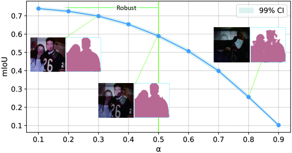
Figure 2. Relationship between mIoU (metric for semantic segmentation) and the weight ($\alpha$) of reflection layer with one visual example. Here CI is the confidence interval. We find that semantic estimation is robust in the observations with a relatively low weight of the reflection layer.

Our motivation is that if the background layer semantic information is provided or can b estimated, we can use it to help separate the background layer from the input image. In other low-level vision tasks to recover the clean image from the interference, the interference layer to be removed is usually largely different from the image layer and contains no semantic object information, e.g., noise, hazy volume, rain streaks. Unlike these tasks, in reflection removal, the reflection layer to be removed is also a reflected scene, which causes difficulty in estimating the background semantics. Therefore, it is important to see how the reflection affects the estimation of background semantics.

We try an empirical study to test the robustness of semantic segmentation estimation against different intensity levels of reflection. We randomly sample images from the Pascal VOC dataset (Everingham et al., [n. d.]), where the ground truth of semantic label is provided in 20 categories. Based on it, we synthesize the image with reflections by linearly blending two images using $\mathbf{I}=(1-\alpha)\mathbf{B}+\alpha\mathbf{R}$, where larger $\alpha$ can simulate the reflection layer with stronger intensity. In total, we sample and generate $5000\times 9$ sets of images with $\alpha=0.1,0.2,\dots,0.9$. Fig. 2 illustrates the relationship between semantic segmentation quality and the weight of reflection layer.

Statistical results have shown that semantic estimation is relatively robust when the weight of reflection layer is below 50%. When the weight is bigger than 50%, such reflections would be taken as extreme cases, which might contain 1) reflection layer is too strong or 2) background layer contains no salient object (and leads texture-less transmission layer). In this work, following all previous methods  (Fan et al., 2017; Zhang et al., 2018), we make a similar assumption and address the cases with moderate reflection strength and the background. The extreme cases with intense reflections are considered as limitations of our method and leave such cases as our future directions.

3.2. Multi-task Learning for Simultaneous Reflection Removal and Semantic Estimation

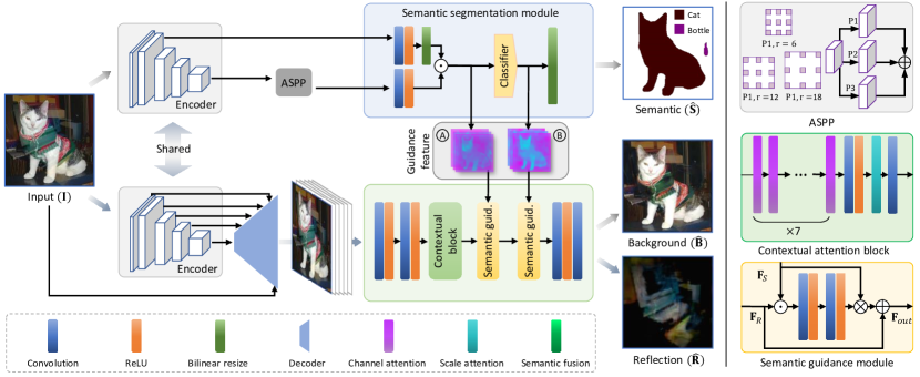
Figure 3. An overview of our proposed SGR²N. Left: For the input image I, we first extract features via the Shared Encoder, and estimate the semantic map $\mathbf{S}_{B}$ of the background through Semantic segmentation module. Next, the semantic information is used to guide the Reflection separation through a semantic guidance module. Finally, background (B) and reflection (R) are estimated from the separation module. Right: From top to down: the architecture of ASPP module, contextual attention block, and semantic guidance module.

Given an input image with reflection interference, we perform two tasks: (1) Extracting background semantic map $\mathbf{S}_{B}$ from input $\mathbf{I}$, and (2) Recovering background layer $\mathbf{B}$ (also reflection layer $\mathbf{R}$) from input $\mathbf{I}$ along with the semantic information ($\mathbf{S_{B}}$) obtained in the first task. To this end, we propose the semantic guide reflection removal network (SGR²N), in which a novel semantic guidance module is proposed to link semantic segmentation and reflection removal together. Our method can work adaptively using semantic information as guidance for reflection removal.

3.2.1. Architecture design.

Our SGR²N layout is illustrated in Fig. 3, containing a Shared Encoder, a Semantic segmentation module, and a Separation module with Semantic guidance. Given the input image, Shared Encoder aims to extract rich features from different stages of the backbone for semantic segmentation task and reflection removal task. Following (Chen et al., 2018), we use ResNet-101 (He et al., 2016) as the backbone, in which intermediate features from different stages are taken as outputs. Semantic segmentation module estimates the semantic map of the input. We follow the DeepLabv3+ (Chen et al., 2018) and move its ASPP module to the decoder. We use the semantic classifier to predict the semantic map of the input image. The semantic classifier is constructed by a $1\times 1$ convolutional layer and a softmax activation layer. It maps the feature into the semantic predictions (with the shape of $[B,N,H,W]$, where $N$ is the number of semantic labels). The intermediate features before/after the classifier are used as guidance for reflection separation.

Separation module utilizes the fused features as input and tries to recover the corresponding background and reflection with semantic guidance. In this module, we use contextual attention to get richer information firstly. This module is proved effective in low-level vision tasks in (Wei et al., 2019). We bring a similar architecture from (Wei et al., 2019) but with fewer channel attention layers.

Semantic guidance for reflection removal. We carefully design a semantic guidance module to use semantic information as guidance for reflection removal. As shown in Fig. 3, the detailed design is as follows. (1) Selection of guidance features. We choose the mid-level feature is because it contains the most informative features from the semantic segmentation module. As illustrated in Fig. 3, we adopt the intermediate features (\small{A}⃝ and \small{B}⃝) of semantic segmentation module. These intermediate features ensure the guidance contains the soft object’s attentions for reflection removal. In detail, a) \small{A}⃝ contains all information about high-level information (generated by ASPP module) and low-level feature (from the output the second residual block of the encoder). b) \small{B}⃝ contains all the features of the segmentation result. (2) Fusing strategy of guidance. The underlying design principle is that we use semantic information to make the network focus on meaningful objects for reflection separation. One of the best ways is to use an attention mechanism to introduce semantic information across channels (Hu et al., 2018). We use the commonly used attention operation for implementation. Based on the standard attention layer, we further get a richer structure by making it within a residual block, which can also avoid a dramatic increase of the trainable parameters.

Here we use two semantic guidance blocks to use mid-level and high-level semantic features to guide reflection removal. Specifically, let $\textbf{F}_{R}$ denote original features produced by the former network layer, $\textbf{F}_{S}$ denote the semantic feature map produced by the semantic estimation module. $\textbf{F}_{S}$ mainly provides contextual attention to the image. Mathematically, the semantic guidance module uses semantic feature $\textbf{F}_{S}$ as guidance for original features $\textbf{F}_{R}$ as follows:

(2) $$\textbf{F}_{out}=\textbf{V}\otimes\textbf{F}_{S}\oplus\textbf{F}_{R},\quad\textbf{V}=\tau(\textbf{w}_{v1}*\tau(\textbf{w}_{v2}*\textbf{K}+\textbf{b}_{v2})+\textbf{b}_{v1}),\quad\textbf{K}=\textbf{F}_{R}\odot\textbf{F}_{S},$$

where $\tau$ is ReLU activation function, $\textbf{w}_{v1},\textbf{b}_{v1},\textbf{w}_{v2},\textbf{b}_{v2}$ are learnable parameters. For the regions with no semantic information, the semantic guidance module will yield the $\textbf{F}_{R}$ directly thanks to the residual structure. This design can provide relatively robust guidance for separation.

The output layer of the reflection removal module is a convolution layer with 6 channels. The former 3 channels construct the background layer B, and the remaining channels construct the reflection layer R.

3.2.2. Loss function

As we are jointly performing two tasks, the final multi-task learning (MTL) loss functions are built on reflection removal task and semantic segmentation together.

Reflection removal loss. We use three terms of loss functions for regularizing $\mathcal{L}_{B}$ and $\mathcal{L}_{R}$, which is similar to previous methods (Wei et al., 2019; Yang et al., 2018; Zhang et al., 2018).

1) Feature loss. Inspired by (Zhang et al., 2018; Rad et al., 2019), we define the feature loss based on the features from the Rich Encoder. This design will not introduce extra resources. Take image X as the input of encoder, let $\phi_{l}$ being the feature from the $l$-th stage of Rich Encoder, the feature loss is defined as:

(3) $$l_{feat}=\sum_{l}\lambda_{l}\parallel\phi_{l}(\textbf{X})-\phi_{l}(\hat{\textbf{X}})\parallel_{1},$$

where $\{\lambda_{l}\}$ denotes balancing weight.

2) Pixel loss. Following (Fan et al., 2017; Wei et al., 2019), we compute the differences between the prediction and the ground-truth in pixel-level and gradient level as follow:

(4) $$l_{pix}=\parallel\textbf{X}-\hat{\textbf{X}}\parallel_{1}+\parallel\nabla\textbf{X}-\nabla\hat{\textbf{X}}\parallel_{1},$$

where $\nabla$ is the gradient operator. $\hat{\textbf{X}}$ and X are the network prediction and corresponding ground-truth.

3) Adversarial loss. We further add adversarial loss to make the produced background and reflection look more realistic. We use a discriminator network $D_{\theta}$ and minimize the adversarial loss (Huang et al., 2018), which is defined as

(5) $$l_{adv}=-\log(D_{\theta}(\textbf{X},\hat{\textbf{X}})),$$

where the loss for discriminator network is $l_{adv}^{D}=-\log(1-D_{\theta}(\textbf{X},\hat{\textbf{X}}))-\log(D_{\theta}(\textbf{X},\hat{\textbf{X}}))$.

To summarize, the loss for background ($\mathcal{L}_{B}$) and reflection ($\mathcal{L}_{R}$) are

(6) $$\mathcal{L}_{B} =w_{1}l_{feat}(\hat{\textbf{B}},\textbf{B})+w_{2}l_{pix}(\hat{\textbf{B}},\textbf{B})+w_{3}l_{adv}(\hat{\textbf{B}},\textbf{B}),$$

$$\mathcal{L}_{R} =w_{1}l_{feat}(\hat{\textbf{R}},\textbf{R})+w_{2}l_{pix}(\hat{\textbf{R}},\textbf{R})+w_{3}l_{adv}(\hat{\textbf{R}},\textbf{R}),$$

where we empirically set $w_{1}=0.1$, $w_{2}=1$ and $w_{3}=0.01$ in our experiments.

Semantic segmentation loss. For semantic loss $\mathcal{L}_{S}$, we use cross-entropy as the penalization.

(7) $$\mathcal{L}_{S}=\sum_{j=1}^{K}\sum_{i=1}^{M}\left(-y_{ji}\log{\hat{y}_{ji}}-\left(1-y_{ji}\right)\log{\left(1-\hat{y}_{ji}\right)}\right),$$

where $K$ is the size of training batch, $M$ is the total number of semantic categories. $M=21$ in our synthetic dataset, $\hat{y}$ is the prediction, the ground truth label is $y$.

Total loss. The total loss is the combination of reflection removal loss and segmentation loss.

(8) $$\mathcal{L}=\alpha\mathcal{L}_{B}+\beta\mathcal{L}_{R}+\mathcal{L}_{S},$$

where the hyper-parameters are empirically set as $\alpha=0.5$, $\beta=0.25$.

3.2.3. Implementation details.

The proposed method is implemented via PyTorch (Paszke et al., 2017a), which is available at Github. To make our model converge faster and save training time, we employ ResNet-101 with pre-trained parameters on ImageNet (Deng et al., 2009), whose effectiveness has been proved in (Zhou et al., 2014). Convolution weights are initialized as CZ18 (Chen et al., 2018). Input images are resized to $256\times 256$ before feeding into the network. We train the SGR²N with 500 epochs using the Momentum optimizer (Ilya et al., 2013), which is employed with $\text{momentum}=0.99$, where the cycle learning rate is initially set as 0.007 and decay in every 30000 iterations until 0.0001. The batch size during training is empirically set to 5.

4. Experiments

We first synthesis the semantically annotated dataset. Then we perform rigorous ablation studies to analyze the effect of different parts of the SGR²N. We evaluate our semantic guided reflection removal method quantitatively and qualitatively on single image reflection removal against previous methods. Next, we make additional experiments on how the intensity of reflection layer affects the final performance of the semantic segmentation and the reflection removal task. Finally, we show applications of our model and make a discussion on failure cases.

4.1. Semantic Reflection Dataset Generation

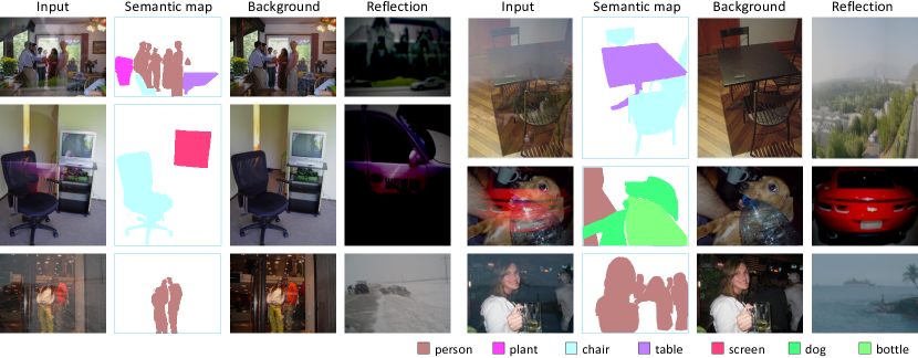
Figure 4. Illustration of the generated semantic reflection dataset. There are abundant annotations with different semantic meanings for each input image. Here we show three input images with over-smoothness reflection (left-1, left-2, and right-2), the other input images are contaminated by reflection with ghost effect.

To train the SGR²N, a training set with semantic annotations is needed. However, existing datasets (Fan et al., 2017; Wan et al., 2017; Zhang et al., 2018) for reflection removal are all lack semantic annotations. On the other hand, it’s labor-consuming to label semantic annotations for the existing reflection removal dataset. Therefore, we generate the reflection removal dataset with semantic labels. In detail, there are four types of aligned data in each group of the proposed dataset: (1) image with reflection $\mathbf{I}$, (2) clear background $\mathbf{B}$, (3) reflection $\mathbf{R}$, and most importantly (4) semantic labels $\mathbf{S}_{B}$.

To render the realistic reflections, we follow the generation strategy in (Zhang et al., 2018), besides, we add ghost effect (Shih et al., 2015) for more abundant and realistic cases. For semantic labels, we generate the dataset on the basis of Pascal VOC (Everingham et al., [n. d.]), which provides semantic annotations. The visual samples of the generated dataset are illustrated in Fig. 4. The generated dataset contains 20 categories of objects, and each image contains 2.93 foreground objects with semantic labels on average. Additionally, the comparison with the existing datasets is listed in Table 1.

Table 1. Brief comparison among different datasets.

Dataset	Source	Volume	Reflection layer	Ghost cases	Semantic label
$\mathcal{D}_{BKL}$	Zhang et al. (Zhang et al., 2018)	110
$\mathcal{D}_{SIR^{2}}$	Wan et al. (Wan et al., 2018)	454	$\checkmark$	$\checkmark$
$\mathcal{D}_{syn}$	Ours	31965	$\checkmark$	$\checkmark$	$\checkmark$

4.2. Experimental Setups

We train the SGR²N on our synthetic training set, and then we evaluate the performance on the different test sets. Specifically, we use 29503 images from our generated dataset as the training data. Then we evaluate the trained SGR²N on the synthetic test set, 20 real images from Berkeley dataset (Zhang et al., 2018) and 463 real images from SIR² dataset (Wan et al., 2018). Image is cropped with the size of 224 $\times$ 224 randomly and is flipped randomly as data augmentation. For the compared methods, we use the same dataset for training, unless specifically stated. For evaluation, we use PSNR, SSIM (Zhou et al., 2004) to measure the quality of reflection removal. Although these two metrics are most widely used in low-level vision tasks, they have their limitations during the test. It is mainly because SSIM and PSNR are both sensitive to the intensity variance. After all, they leverage luminance and contrast similarity between two images. Therefore, we further use histogram alignment techniques to better calculate SSIM and PSNR in Sec.4.4. Following recent and popular semantic segmentation papers (Chen et al., 2018; Carion et al., 2020), we use mean Intersection over Union (mIoU) and pixel accuracy of different categories for semantic segmentation.

4.3. Ablation Study

In this section, we evaluate the effectiveness of 1) our multi-task learning architecture, analyze the 2) semantic guidance module and 3) loss functions.

Architecture. To evaluate the effectiveness of our semantic guidance architecture, we remove the multi-task scheme or semantic guidance block and re-train the network under the same condition. We first reconstruct our model with training reflection separation solely and take this version as the baseline, as shown in Fig 5 (a). In this case, the architecture of baseline is similar to previous state-of-the-art methods (Zhang et al., 2018; Wei et al., 2019).

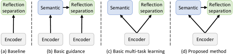
Figure 5. Different settings of the semantic guided reflection removal model. (a) Train semantic segmentation task solely. (b) The basic multi-task learning model in which two tasks share the same encoder. (c) Our final model in which semantic estimation branch shares guidance to reflection removal branch.

We find that reflection cannot be removed in Fig. 6-top (c), and even unpleasant color-shift appears at the area of reflections. Meanwhile, as shown in the third row of Fig. 6-top (c), the reflection layer separated from the input contains nothing meaningful. The reason is that the baseline is a reflection removal network with no semantic awareness.

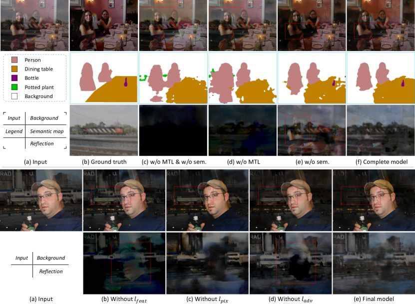
Figure 6. Visual results of ablation studies. Top: Visual comparisons of reflection removal results with different network structures. Bottom: Visual results about the loss functions of the SGR²N.

Semantic guidance block. To evaluate the effectiveness of the semantic guidance block, we conduct additional experiments by adding semantic guidance into the baseline, as illustrated in Fig. 5 (b). Specifically, we train the semantic segmentation network at first, then freeze the semantic segmentation branch and use its decoder to guide reflection separation through semantic guidance block. Table 2 shows the ablation study for architecture. This operation can improve the performance of reflection separation (background/reflection) by $3.03/0.58$ PSNR and $0.007/0.035$ SSIM. The visual results at the top of Fig. 6 (d) show that parts of reflection can be separated from the input, but there are still many residuals that remain on the girl’s faces. The reason why reflection separation cannot significantly benefit from semantic guidance is that semantic information is not accurate enough when it is extracted from the image contaminated directly.

MTL scheme. To verify the contribution of MTL, we use a Basic MTL scheme to jointly optimize semantic segmentation and reflection separation and make these two tasks share the same encoder, which is illustrated in Fig. 5 (c). This effective operation can promote the performance of reflection separation (background/reflection) improved by $3.33/1.93$ PSNR and $0.038/0.116$ SSIM. However, it can be found that the arm of the left girl is mistakenly separated into the reflection layer. As a result, there are many residuals of background on the reflection layer. In the meantime, some parts with semantic meaning of the background are missing.

The performance of reflection separation is further improved by merging semantic guidance with MTL, as illustrated in Fig. 5 (d), which is our final model. Fig 6-top (f) shows clearer background at the region where semantic information guides. More specifically, persons in the background layer become clearer without artifacts on the arm (highlighted with dashed box). Meanwhile, the residuals are removed totally from the reflection layer. The PSNR of background/reflection is improved from $25.22/17.47$ to $26.02/18.51$ and SSIM is improved from $0.859/0.538$ to $0.875/0.592$. The semantic segmentation achieves better results by simultaneously learning to reflection removal.

We further explore the relationship between semantic segmentation and different architectures. The quantitative comparison is reported in the 4-th column of Table 2 and one group’s results are illustrated in Fig. 6-top. Without multi-task learning, we find that the bottle in the input image cannot be recognized and separated correctly due to the reflection, which is shown in Fig. 6-top (d) and (f). It can be seen that the proposed MTL and semantic guidance not only can consistently improve the reflection removal performance on three datasets but also improve the performance of semantic segmentation (MTL: $\uparrow 0.151$ mIoU, Final version: $\uparrow 0.189$ mIoU). These quantitative results show the effectiveness of our proposed architecture.

Table 2. Segmentation performance of mIoU and reflection removal performance of SSIM and PSNR on the synthesized and real test set. MTL: multi-task learning. Guid.: semantic guidance.

	Architecture		$\mathcal{D}_{syn}$				$\mathcal{D}_{BKL}$		$\mathcal{D}_{SIR^{2}}$
Method	MTL	Guid.	mIoU	Pixel acc.	SSIM	PSNR	SSIM	PSNR	SSIM	PSNR
Baseline			0.395	75.33	0.821	21.67	0.721	18.79	0.819	21.68
SGR2N	$\checkmark$		0.546	84.68	0.859	25.22	0.801	19.98	0.877	22.98
SGR2N		$\checkmark$	0.395	75.33	0.833	24.70	0.799	21.02	0.867	22.62
SGR2N	$\checkmark$	$\checkmark$	0.584	88.79	0.875	26.02	0.812	22.46	0.893	23.81

Analysis of different loss functions. To analyze how each loss contributes to the final performance of our network on reflection separation, we conduct additional experiments on the feature loss Eqn. (3), the pixel loss Eqn. (4), and adversarial loss Eqn. (5). To make a detailed ablation study on feature loss $l_{feat}(\hat{\textbf{B}},\textbf{B})$, we conduct ablation studies as follow:

1. Totally remove the loss term. We remove $l_{feat}(\hat{R},R)$ from the total loss, then $\hat{\textbf{R}}$ is generated through $\textbf{I}-\hat{\textbf{B}}$.

2. Replace the loss term. We replace $l_{feat}(\hat{\textbf{B}},\textbf{B})$ with the L1 difference between B and $\hat{\textbf{B}}$.

The $l_{feat}(\hat{\textbf{R}},\textbf{R})$ is useful to the performance of reflection removal. To demonstrate this, we have made a similar ablation study on it. The quantitative results are reported in Table 3. Note that the results of ablation studies on $l_{feat}(\hat{\textbf{R}},\textbf{R})$ are marked with ${\dagger}$.

When we remove the feature loss $l_{feat}$, there are many residuals of reflections on the background layer, and some parts of the man’s face are taken as reflection mistakenly, as shown in Fig. 6-bottom (b). The reason can be that $l_{feat}$ contains many perceptual constraints, which can constrain the low-level, mid-level, and high-level information of the background and reflection layers in the latent space (Zhang et al., 2018). When we remove the $l_{pix}$, some color-shifting occurs on the image, e.g., the man’s shirt becomes darker, and the man’s skin looks slightly over-saturated; the reason is that the $l_{pix}$ constrains the pixel-level appearance of the image. The adversarial loss $l_{adv}$ further helps recover more natural backgrounds and reflections, as shown in the bottom of Fig. 6 (d) and (e).

The quantitative comparisons are shown in Table. 3. In the first row, we take the state-of-the-art method (Zhang et al., 2018) as reference. Removing different loss terms from the total loss, we test the SGR²N under the same condition. In the second row, we remove feature loss and adversarial loss and take this model as a baseline. It can be found that the reference method (Zhang et al., 2018) performs better than our baseline. These results are reasonable because method (Zhang et al., 2018) adopts various loss functions, viz. feature loss, adversarial loss, and exclusive loss. Adding adversarial loss into the objectiveness, the performance of background/reflection improves $0.01/0.055$ SSIM and $0.42/1.25$ PSNR, and our method with these settings gets comparable results to the state-of-the-art. The 4-th line of Table 3 shows that feature loss can improve $0.047/0.107$ SSIM and $3.48/1.81$ PSNR. As for changing the $l_{feat}(\hat{\textbf{R}},\textbf{R})$ to L1 loss, the performance is also decreased. For background layer, SSIM: 0.875$\to$0.871, PSNR: 26.02$\to$25.89. The performance drops steadily without pixel loss. The combination of feature loss and adversarial loss can further boost the performance to $0.875/0.592$ SSIM and $26.02/18.51$ PSNR. As shown in the last row, numerical results on other real benchmark datasets also show the combination of different loss terms achieves the best performance comprehensively. Visual results in a Fig. 6 also show the clearer background and reflection layers, especially in the region with dashed boxes.

Table 3. Loss ablation experiments on the test set.

	$\mathcal{D}_{syn}$		$\mathcal{D}_{BKL}$		$\mathcal{D}_{SIR^{2}}$
Method	SSIM	PSNR	SSIM	PSNR	SSIM	PSNR
Reference  (Zhang et al., 2018)	0.835	22.66	0.807	22.37	0.847	22.82
Baseline	0.824	21.69	0.801	21.56	0.849	22.73
SGR2N (w/o $l_{pix}$)	0.840	23.26	0.791	20.25	0.811	21.37
SGR2N (w/o $l_{feat}$ (a))	0.834	22.93	0.808	22.37	0.874	23.24
SGR2N (w/o $l_{feat}$ (b))	0.860	24.99	0.811	22.46	0.891	23.80
SGR2N (w/o $l_{feat}$ (a)${\dagger}$)	0.861	25.58	0.810	22.41	0.888	23.61
SGR2N (w/o $l_{feat}$ (b)${\dagger}$)	0.871	25.89	0.812	22.46	0.894	23.80
SGR2N (w/o $l_{adv}$)	0.872	25.17	0.810	22.75	0.893	23.87
SGR2N	0.875	26.02	0.812	22.46	0.893	23.81

4.4. Comparison with the State-of-the-Art Methods

In this section, we compare our SGR²N against state-of-the-art methods including optimization-based approaches (LB14 (Li and Brown, 2014), AN17 (Arvanitopoulos et al., 2017), and YM19 (Yang et al., 2019)) and the learning-based methods (CEILNet (Fan et al., 2017), CRRN (Wan et al., 2018), BDN (Yang et al., 2018), ZN18 (Zhang et al., 2018), ERRNet (Wei et al., 2019), WT19 (Wen et al., 2019) and ICBLN (Li et al., 2020c)). For a fair comparison, we finetune these models on our training dataset if the training code has been published. We have also provided the numerical results of pretrained IBCLN (termed as IBCLN-p).

Synthetic images. Our synthetic test set contains 1969 {input, background, and reflection} triplets and corresponding semantic maps. We train all the existing methods on our synthetic training set if they were CNNs based and provided training code. Then we make quantitative and qualitative comparisons among these methods and ours.

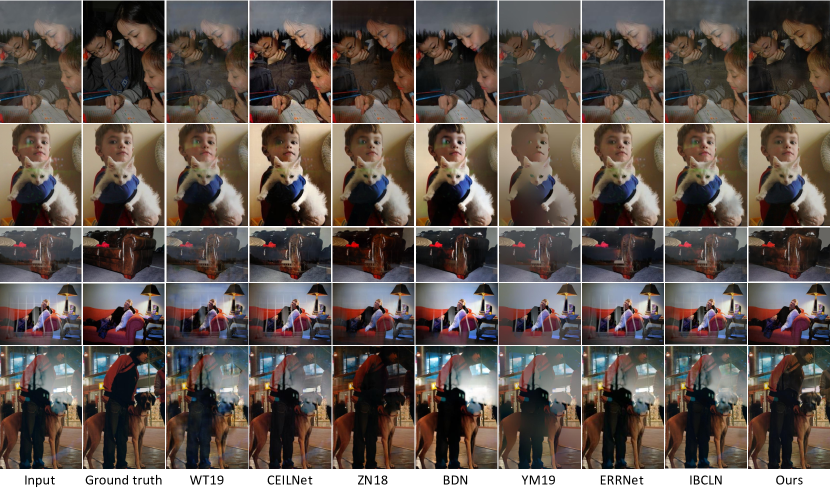
Figure 7. Visual background layers comparison of our method with four previous methods, evaluated on the synthetic dataset $\mathcal{D}_{syn}$. Our model generates superior results with cleaner local details.

The quantitative results are shown in Table 4. The fine-tuned version of previous methods shows better numerical performance than the pre-trained version (Table 4 IBCLN-p v.s IBCLN). We show stronger quantitative performance over previous works on both synthetic data, meanwhile, our method reaches a relatively fast runtime.

Fig. 7 shows the qualitative results of different methods. It can be found that the state-of-the-art methods cannot remove reflection totally, while these reflections can be removed easily with semantic understanding via our SGR²N. More specifically, WT19 (Wen et al., 2019) cannot remove reflection on the area which has obvious semantic meaning. CEILNet (Fan et al., 2017) can remove some reflections, however, it can be found other artifacts appear on the boy’s face (the bottom of 5-th column of Fig. 7). ZN18 (Zhang et al., 2018) can remove most reflections, but unpleasant color-shifting occurs on the girl’s face. BDN (Yang et al., 2018) enhances the color of the input image and smooths the reflection area, but the reflections aren’t removed apparently. YM19 (Yang et al., 2019) over-smooths the input image and outputs unrealistic results. ERRNet (Wei et al., 2019) can produce a relatively clean background layer, but there are still some reflection residuals on the output. To summarize, our method produces the most compelling results with correct removal and cleaner local details. Furthermore, the previous methods show obvious quantitative performance margins below the proposed method on synthetic data. It can be explained that plenty of semantic objects greatly boosted the performance of reflection removal through our method.

Table 4. Quantitative comparison and runtime results among our method and other 8 prior works on $\mathcal{D}_{syn}$. Our model gets stronger quantitative performance over previous works and reaches relatively a fast runtime.

		Background		Reflection
Method	GPU	SSIM	PSNR	SSIM	PSNR	Runtime (s)
LM14 (Li and Brown, 2014)		0.779	19.19	0.3444	15.43	0.475
AN17 (Arvanitopoulos et al., 2017)		0.781	19.23	-	-	99.38
CEILNet (Fan et al., 2017)	$\checkmark$	0.792	21.00	-	-	0.195
BDN (Yang et al., 2018)	$\checkmark$	0.824	19.67	0.345	11.29	0.024
ZN18 (Zhang et al., 2018)	$\checkmark$	0.835	22.66	0.463	17.22	0.332
YM19  (Yang et al., 2019)		0.796	20.35	-	-	0.270
ERRNet  (Wei et al., 2019)	$\checkmark$	0.827	22.71	-	-	0.719
WT19  (Wen et al., 2019)	$\checkmark$	0.818	21.38	-	-	0.422
IBCLN  (Li et al., 2020c)	$\checkmark$	0.817	22.09	0.407	13.40	0.189
IBCLN-p (Li et al., 2020c)	$\checkmark$	0.808	21.88	0.371	13.29	0.189
SGR2N	$\checkmark$	0.878	26.02	0.592	18.51	0.132

Real images. To make a fair comparison, if the previous methods’ pretrained models are published, we use the published model directly for comparison. Otherwise, We fine-tune these models on the real images under the same setting. The test set of Berkeley real image contains 20 {input, background} pairs, which are collected behind a portable glass (Zhang et al., 2018).

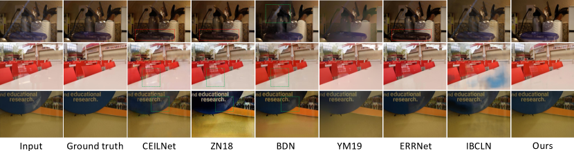
Figure 8. Visual background layers comparison of our method with 6 previous state-of-the-art methods, evaluated on the real images.

We further conduct comparisons on SIR² (Wan et al., 2018), which contains three sub-datasets. These three sub-datasets are captured under different conditions: (1) 20 controlled indoor scenes composed by solid objects; (2) 20 different controlled scenes on postcards; and (3) 55 wild scenes with ground truth. In the following, we compute the average PSNR/SSIM of these three sub-datasets for different methods.

Fig. 8 shows the qualitative comparisons on the test set. Our method can handle images with complex semantic information. Furthermore, our method can generate cleaner background than other methods. The first row shows one visual comparison among state-of-the-art methods on Berkeley test set and the last two rows show the results on SIR² dataset. For the visual results on the first row, we observe that CEILNet (Fan et al., 2017), ZN18 (Zhang et al., 2018), and ERRNet (Wei et al., 2019) can produce clean background. However, some details of color are missing, as illustrated in the red box. BDN (Yang et al., 2018) and YM19 (Yang et al., 2019) can preserve the color detail of the input image, but BDN cannot remove reflection totally (as shown in the green boxes). YN19 produces over-smoothed images which are not realistic. Our method can overcome such limitations through semantic understanding and can reconstruct clean and correct background images. ICBLN introduces additional artifacts on the image, such as the white table suffered seriously in the second row.

Table 5 summarizes the results of all competing methods on these two real benchmarks viz.Berkeley test and SIR² benchmark. Note that Berkeley test images only provide the ground-truth for backgrounds; thus it is not adaptable to evaluate the performance on reflection images. We find in this dataset, there are semantic categories that are unseen in the training set. The semantic information cannot be used to guide reflection removal. In this situation, the performance of reflection removal decreases slightly. One possible way for this is to annotate more kinds of semantic labels. Even though, our SGR²N still achieves comparable results. Meanwhile, our model shows superior performance on SIR² benchmark. Because the codes of Ma et al. (Ma et al., 2019) and Kim et al. (Kim et al., 2020a) have not been published yet, we compare the numerical results (which are from their published paper) on the subset of the SIR² (i.e.Wild Scenes). As reported in the SIR* in Table 5, our method shows consistently effective results.

Table 5. Quantitative comparison results between the proposed method and other state-of-the-art methods on two real benchmarks. Note that best results are marked in bold, and the second places are underlined. Note that SIR²* dataset denotes that only part of SIR² (i.e.Wild scene) is used.

		Background		Reflection
	Method	SSIM	PSNR	SSIM	PSNR
$\mathcal{D}_{BKL}$	Input (Reference)	0.694	17.66	-	-
	LM14 (Li and Brown, 2014)	0.563	17.54	-	-
	AN17 (Arvanitopoulos et al., 2017)	0.586	17.55	-	-
	CEILNet (Fan et al., 2017)	0.710	18.77	-	-
	BDN (Yang et al., 2018)	0.656	18.58	-	-
	ZN18 (Zhang et al., 2018)	0.807	22.37	-	-
	YM19  (Yang et al., 2019)	0.640	18.05	-	-
	ERRNet  (Wei et al., 2019)	0.811	22.84	-	-
	WT19  (Wen et al., 2019)	0.795	19.76	-	-
	IBCLN  (Li et al., 2020c)	0.762	21.86	-	-
	RAGNet  (Li et al., 2020a)	0.793	22.95	-	-
	SGR2N	0.812	22.46	-	-
$\mathcal{D}_{SIR{{}^{2}}}$	Input (Reference)	0.801	20.12	0.410	8.72
	LM14 (Li and Brown, 2014)	0.718	17.01	0.455	15.21
	AN17 (Arvanitopoulos et al., 2017)	0.716	18.96	-	-
	CEILNet (Fan et al., 2017)	0.819	21.65	-	-
	BDN (Yang et al., 2018)	0.842	21.76	0.270	8.77
	ZN18 (Zhang et al., 2018)	0.847	22.82	0.403	18.52
	YM19  (Yang et al., 2019)	0.831	21.32	-	-
	CRRN  (Wan et al., 2018)	0.884	22.86	-	-
	ERRNet  (Wei et al., 2019)	0.890	23.59	-	-
	WT19  (Wen et al., 2019)	0.827	21.50	-	-
	IBCLN  (Li et al., 2020c)	0.885	23.53	0.392	14.89
	IBCLN  (Li et al., 2020c)-p	0.884	23.56	0.338	14.57
	SILS  (Liu and Lu, 2020)	0.821	20.47	0.425	19.31
	RAGNet  (Li et al., 2020a)	0.890	23.93	0.511	17.65
	SGR2N	0.893	23.81	0.607	19.54
$\mathcal{D}_{SIR{{}^{2}}}$*	Input (Reference)	0.868	22.73	0.441	10.15
	Ma et al. (Ma et al., 2019)	0.903	24.48	-	-
	Kim et al. (Kim et al., 2020a)	0.905	25.55	-	-
	IBCLN  (Li et al., 2020c)	0.886	24.70	0.322	13.40
	IBCLN  (Li et al., 2020c)-p	0.886	24.71	0.320	13.31
	SILS  (Liu and Lu, 2020)	0.833	21.01	0.444	14.35
	RAGNet  (Li et al., 2020a)	0.880	25.52	0.492	15.15
	SGR2N	0.905	25.93	0.544	17.10

Our method also performs well for images with complex semantics. As illustrated in Fig. 9 and Fig. 10, our method can handle images with complex semantic information. It can be found that even if there are more than 6 kinds of semantic objects in the input, our method can still perform well in this case. The semantic map is generated through DETR (Carion et al., 2020) for reference.

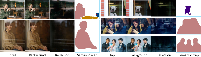
Figure 9. More results on real images. The input images are from CEILNet (Fan et al., 2017).

Fig. 9 illustrates more visual results on real images, which are provided by (Fan et al., 2017). It can be observed that the proposed method generates clean backgrounds and clear reflections. Meanwhile, the semantic map is predicted correctly. These results show that our method can generalize well on various real scenes across different datasets.

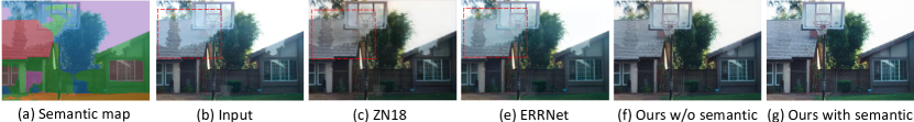
Figure 10. Comparisons on scenes with complex semantics. Our method gets better visual quality than the completed methods. The performance is further improved with semantic guidance.

Alleviate the intensity sensitivity of SSIM and PSNR. We notice in the qualitative comparison that the resulting images given by some comparing approaches are slightly darker than the ground truth. It may affect the SSIM and PSNR result. Therefore, we align the lightness-histogram of all resulting images to be the same as the input such that the numerical comparison will not be biased by such as the brightness of the images.

To handle this, we have conducted an additional experiment as follows:

1) Histogram alignment. We align the lightness-histogram of all resulting images to be the same as the input image. In detail, we first convert the resulting image and input from RGB space to HSV space. Since the V channel is highly related to the brightness, we align the V channel of the resulting image to the V channel of the input image. In the next, the original V channel of the resulting image is replaced with the result from the last step. Finally, we convert the modified resulting image back to RGB space. The visual results and alignment curves are illustrated in Figure 11. After histogram alignment, the resulting image becomes brighter.

2) Performance test. We then computed the SSIM and PSNR between the aligned image and the corresponding ground truth. The alignment results will affect the PSNR and SSIM, visual results are shown in Figure  12. Quantitative results are shown in Table 6. As reported, the performances of all methods are slightly boosted in the synthetic dataset. Our method consistently generates better results over different datasets and layers.

In summary, after brightness alignment, our method still outperforms other competed methods, especially in $\mathcal{D}_{BKL}$.

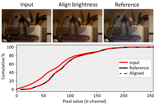
Figure 11. Visual results of lightness-histogram alignment. The top row shows the visual comparison among the source image, the brightness matched image, and the reference image. The bottom row shows the cumulative result vs pixel value curve. It is observed that the brightness histogram of the matched image is closely aligned to the reference image.

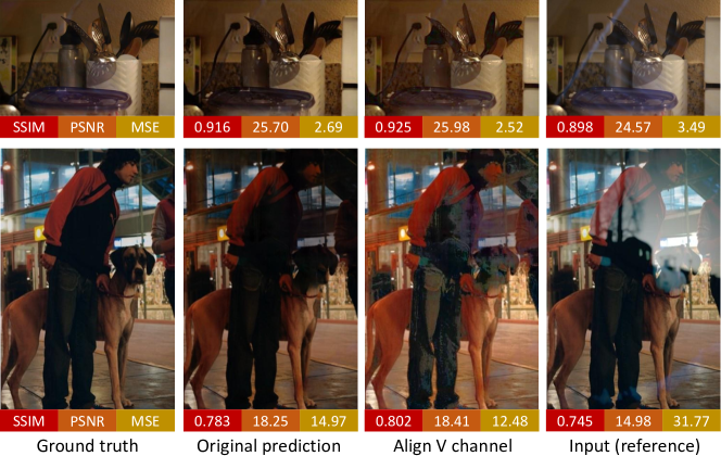
Figure 12. Comparison of before/after brightness-histogram alignment. SSIM, PSNR, and MSE ($\times 1e3$) are used to measure the similarities between the predicted image and ground truth.

Table 6. Quantitative comparison results of background layer among our method and other 8 prior works, with and without brightness alignment to the input image. Our model gets consistently stronger quantitative performance over previous works.

	Synthetic dataset				Real dataset (Berkeley)
	Original		Align brightness		Original		Align brightness
Method	SSIM	PSNR	SSIM	PSNR	SSIM	PSNR	SSIM	PSNR
LM14	0.779	19.19	0.788	19.67	0.563	17.54	0.544	16.67
AN17	0.781	19.23	0.792	19.59	0.586	17.55	0.541	17.02
CEILNet	0.792	21.00	0.819	21.90	0.710	18.77	0.778	22.09
BDN	0.824	19.67	0.827	20.08	0.656	18.58	0.670	19.21
ZN18	0.835	22.66	0.844	24.35	0.807	22.37	0.819	22.80
YM19	0.796	20.35	0.799	21.80	0.640	18.05	0.657	19.11
ERRNet	0.827	22.71	0.838	23.79	0.811	22.84	0.825	22.90
WT19	0.818	21.38	0.823	22.01	0.795	19.76	0.787	19.74
IBCLN	0.817	22.09	0.819	23.17	0.762	21.86	0.780	22.04
SGR2N	0.878	26.02	0.880	26.99	0.812	22.46	0.830	22.99

Inference time. We further test the running time of prior works and ours and present the result in the last column of Table 4. We test different approaches on $\mathtt{Ubuntu18.04}$, with an Intel ®$\text{Core}^{TM}$ i7-7700 CPU and a $\mathtt{GeForceGTX1080}$ GPU card. The comprehensive comparison is illustrated in Fig. 13. In detail, methods LM14 (Li and Brown, 2014), AN17 (Arvanitopoulos et al., 2017). and YM19 (Yang et al., 2019) are tested on CPU with Mathlab 2017b (MATLAB, 2010). The other methods are tested on GPU: CEILNet (Fan et al., 2017) is implemented through Torch (Collobert et al., 2011). YG18 (Yang et al., 2018), BDN (Yang et al., 2018), ERRNet (Wei et al., 2019), and WT19 (Wen et al., 2019) are implemented via PyTorch (Paszke et al., 2017b). Method ZN18 (Zhang et al., 2018) is implemented through Tensorflow. We find our method decreased the computational cost, in terms of parameters and inference time. To demonstrate this, we have conducted additional comparisons between our methods and the other two state-of-the-art methods (Zhang et al., 2018; Wei et al., 2019). Detailed results are listed in Table 8 supplemental material.

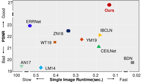
Figure 13. Comparison with previous methods: PSNR versus single image runtime. Numbers are taken from Table 4. Our method outperformed previous methods in a comprehensive way.

4.5. Relationship Between the Semantic Segmentation and Reflection Removal

To understand how the quality of semantic information affects reflection removal, we conduct an additional experiment to more deeply explore the relationship between semantic guidance and reflection removal. The experiment is organized as follows:

1. Reflection removal with accurate semantics as guidance. We use the features from the semantic estimation branch of our final model. In this case, semantic features are correctly computed.

2. Reflection removal without semantic guidance. In this case, we remove the semantic features directly.

3. Reflection removal with wrong semantics as guidance. To demonstrate the effect of wrong semantics, we pre-compute the semantic features of another image. Then we replace the input of the semantic guidance module with these features. In this way, wrong semantics are taken as guidance for reflection removal.

The visual results are illustrated in Fig. 14. Then one can find the results that

1. When accurate semantics are used as guidance, which is illustrated in Fig. 14 (b), reflection can be well removed and the background tends to be clean and of high quality.

2. When the semantic information is removed, as shown in Fig. 14 (c), the reflection can be still removed from the mixed image. But there may leave few contextual residuals of reflection, as illustrated in the dashed box.

3. When the wrong semantic features are used to guide reflection removal, as shown in Fig. 14 (d)-(e), the results suffer some artifacts.

In summary, semantic information is important to reflection removal, and different semantics will affect the reflection separation performance. In addition, the quality and accuracy of the semantic information are jointly optimized with our method. As shown in Fig. 15(b), the semantic estimation is relatively robust in most cases.

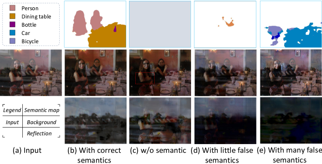
Figure 14. The effect of semantic guidance quality in final reflection removal results. (b) with correct semantic guidance, (c) without semantic guidance, (d)-(e) with wrong semantic guidance.

4.6. Exploration of Performance v.s the Reflection Strength

In this section, we make experiments on the relationship between the SGR²N performance and the strength level of the reflection layer. We generate a series of image quadruples of $\{\mathbf{I}_{t},\mathbf{B}_{t},\mathbf{R}_{t},\mathbf{S}_{t}\}^{N}_{t=1}$, where $\mathbf{I}=(1-\alpha)\mathbf{B}+\alpha\mathbf{R}$, where $\alpha$ is a reflection strength-relevant parameter. We set $\alpha=0.1,0.2,\dots,0.9$ in this experiment to generate 9 groups of datasets, respectively. Here images are randomly selected from Pascal VOC (Everingham et al., [n. d.]). Each group contains 1000 quadruples (I, B, R, and S) for training and 200 quadruples for test. For each group, we train and test our method under the same condition. Then we compare the reflection removal and semantic performance (pixel accuracy and mIoU) v.s $\alpha$ through different settings. We compare the final mIoU of DeeplabV3+ (Chen et al., 2018) (pretraiend on PascalVOC dataset) and the final PSNR of our baseline (Zhang et al., 2018) on such images.

As presented in Fig. 15(a), the proposed SGR²N performs a higher score than the baseline in most cases with different $\alpha$ values. Furthermore, the SGR²N performs a more robust result to different intensities of reflection layer, as illustrated in Fig. 15(b). We find that reflection influences semantic accuracy slightly when reflection strength is lower than 0.5. Otherwise, the reflection will influence semantic accuracy. Note that such scenarios are also hard cases for reflection removal because the input image is dominated by reflection scenes.

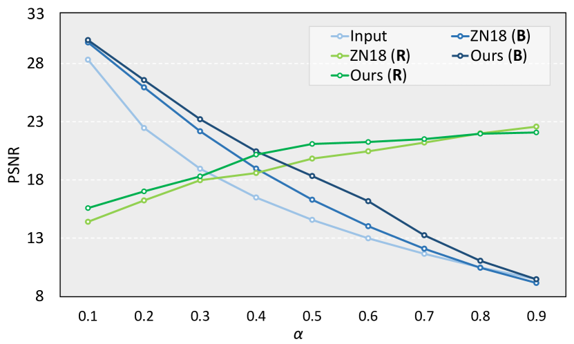
(a) Reflection removal results (PSNR) in images with different reflection intensities.

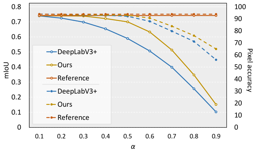
(b) Semantic segmentation results (mIoU and pixel accuracy) in images with different reflection intensities.

Figure 15. Results of reflection removal (a) and semantic segmentation (b) v.s different reflection strengths.

4.7. Failure Cases and Discussion

Although the SGR²N achieves the state-of-the-art on these three datasets, there are challenging cases illustrated in Fig. 16. One of the challenging scenarios where the reflection in the input is too strong, the background is contaminated heavily and our model may not separate layers successfully. The cascade update scheme ICBLN (Li et al., 2020c) can not separate the reflection correctly. As shown in the first row of Fig. 16, the low-frequency part of the input image is incorrectly separated into reflection layer. Note that reflections cannot be totally removed by these methods, but still, our result is superior to (Zhang et al., 2018) (e.g., the person in the background is more distinguishable and the reflection layer is clearer to the other two state-of-the-art methods).

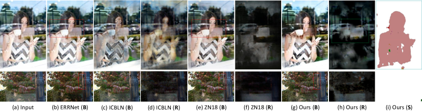
Figure 16. Two typical failure cases for our method. (1) The reflection intensity is too strong. (2) The input image lacks meaningful semantic information. Our method can still produce comparable and even superior results than the state-of-the-art methods ERRNet (Wei et al., 2019), IBCLN (Li et al., 2020c) and ZN18 (Zhang et al., 2018).

4.8. Extend Applications

We extend the proposed method on object detection. To verify how reflection removal benefits object detection, we conduct additional experiments by using the state-of-the-art objection detection approach YOLO-v3 (Redmon and Farhadi, 2018). Specifically, we generate 500 groups of images with bounding box annotations based on Pascal VOC (Everingham et al., [n. d.]). We use mean average precision (mAP) over all 20 classes as evaluation metrics for objection detection. Quantitative and qualitative comparisons are shown in Table. 7 and Fig. 17, respectively. Table. 7 shows that the mAP in reflection contaminated image drops over 12%, and the results are greatly improved after reflection removal. The detection results on reflection-removed output $\hat{\textbf{B}}$ hold higher numerical performance and better visual appearance. In detail, as shown in Fig. 17, the person can be predicted accurately when the reflection is removed. We find the detection results on our method are relatively accurate because our method produces more clean background than compared method.

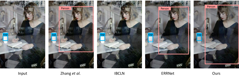
Figure 17. We run YOLO-v3 (Redmon and Farhadi, 2018) on object detection to verify the effectiveness of SGR²N. Left: the visual result of images with reflection; Right: the results of predicted background from the different methods.

Table 7. Pascal VOC object detection results. The mAP of the clear background is used as the baseline.

Input	B	I	$\hat{\textbf{B}}$
mAP	47.17	34.75 ($\downarrow$ 12.42%)	42.83 ($\downarrow$ 4.34%)

5. Conclusion and Discussion

In this paper, we have presented an approach to use semantic clues for the task of single image reflection separation. We first explore the relationship between semantic segmentation and reflection removal and applied high-level guidance explicitly. We design a deep encoder-decoder network for image feature extraction and use a semantic segmentation network in parallel. Then with the two kinds of information fused together, our separation network can correctly separate the background layer and reflection layer. We evaluate our method with other prior works extensively on three different datasets. The comparison result shows that our approach can outperform the existing methods both quantitatively and visually on all three datasets. Like other methods, the extreme cases where the reflection layer is too strong or the background layer contains texture-less objects are considered as the limitation of our method and we leave such cases as our future directions.

Online Appendix

Appendix A More Visual Results on Real Benchmark Datasets

We show more visual results in Fig. 18 and Fig. 19 on real benchmark dataset, including $\mathcal{D}_{BKL}$ and $\mathcal{D}_{SIR^{2}}$. Various scenarios with reflections are presented. Here we compare three state-of-the-art reflection removal methods, ZN18 (Zhang et al., 2018), ERRNet (Wei et al., 2019), IBCLN (Li et al., 2020c), SILS (Liu and Lu, 2020), and RAGNet (Li et al., 2020a). In Fig. 18, we find our method generates precise semantic segmentation (S). Also, compared with the other methods, our method yields favorable results. For instance, the reflections on the semantic objects, e.g., vase(first row), the chair (last row), etc., are all removed properly by our method.

We have also presented the visual results on $\mathcal{D}_{SIR^{2}}$ in Fig. 19. This figure contains three types of scenes. From top to down, they are solid object scenes, postcard scenes, and wild scenes. We find out method can generate comparable results when the semantic information is limited, especially in the postcards scenes. When there is some semantic information for guidance, our method produces more favorably visual results than other methods. These results show the flexibility and generalization ability of our framework and semantic guidance module.

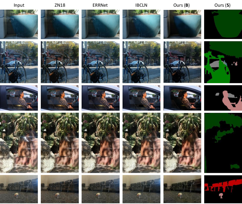
Figure 18. Qualitative comparison among state-of-the-art reflection removal methods and ours over $\mathcal{D}_{BKL}$. Please zoom in on the screen for the details. We have attached our semantic segmentation for reference.

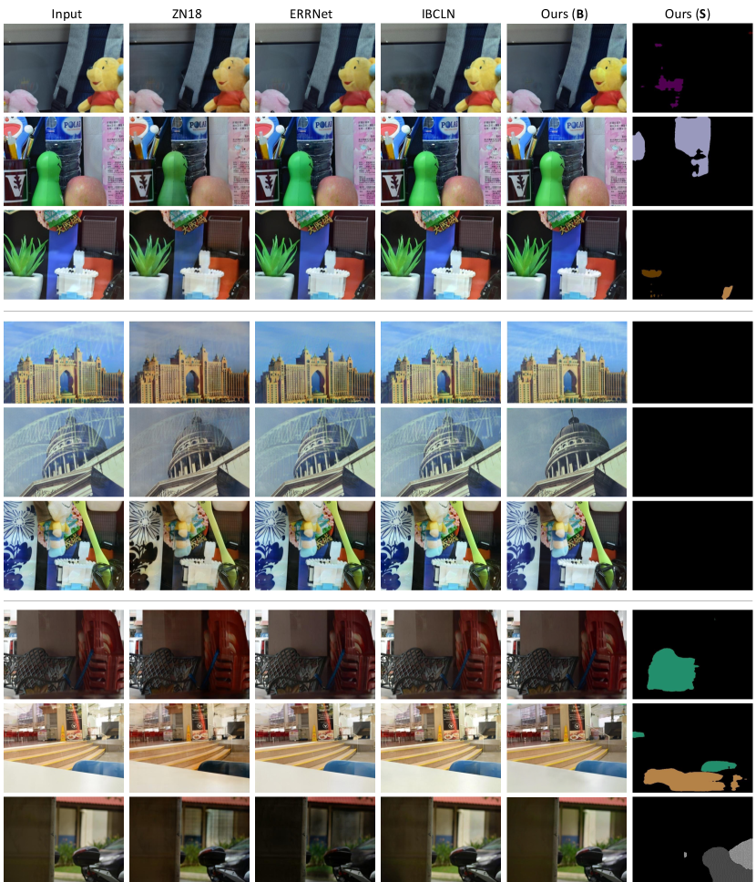
Figure 19. Qualitative comparison among state-of-the-art reflection removal methods and ours over $\mathcal{D}_{SIR^{2}}$. We have attached our semantic segmentation for reference.

Appendix B More Details About the Architecture of Different Methods

Table 8. Number of model parameters and inference time comparison of different methods.

Method	Encoder		Decoder		Discriminator		Total	Inference
	Params(M)	FLOPs(G)	Params(M)	FLOPs(G)	Params(M)	FLOPs(G)	Params(M)	Time (ms)
ZN18 (Zhang et al., 2018)	(VGG-19)		(FCN with dilations)		(5-layer CNNs)		150.34	432
	143.67	19.63	3.90	48.84	2.77	2.71
ERRNet (Wei et al., 2019)	(VGG-19)		(FCN with designed modules)		(12-layer CNNs)		172.55	719
	143.67	19.77	18.95	337.40	9.93	5.31
Ours	(ResNet-101 + ASPP)		(Image + semantic decoder)		(3-layer CNNs)		63.60	132
	57.93	12.87	4.46	41.12	1.21	1.77

As shown in Table 8, ZN18 and ERRNet use VGG-19 as encoder, which uses much more parameters than that in our encoder, i.e., 143.67M and 57.93M. Besides, the sum of parameters in the decoder of ZN18 is 3.90M, and ours is 4.46M, whereas ERRNet uses 18.95M parameters in the decoder. Therefore, our method has fewer parameters in the total model. Furthermore, Our method is also inference faster than these two state-of-the-art methods. More intuitive comparisons among different methods are illustrated in Fig. 13.

Appendix C Extend Applications on Low-level Vision Tasks

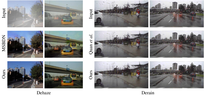
Figure 20. Generalization ability of our method on dehazing and deraining tasks.

Table 9. Quantitative results of our method on dehazing and deraining tasks.

	Dehazing			Deraining
Method	SSIM	PSNR	Method	SSIM	PSNR
Baseline	0.787	23.42	Baseline	0.947	29.02
MSBDN	0.807	24.54	Quan et al.	0.945	28.23
Ours	0.806	24.93	Ours	0.984	34.70

To further show the generalization ability of our method, we have conducted additional experiments on dehazing and deraining. Visual results have been shown in Fig. 20. Numerical results are reported in Table 9. Here we train our model on standard RESIDE dataset (Li et al., 2018) for dehazing and PBRR dataset (Liu et al., 2019; Hao et al., 2019) for deraining, respectively. We generate pseudo semantic labels via DETR (Carion et al., 2020). Here we conduct the recent dehazing method (MSBDN (Dong et al., 2020)) and deraining approach (Quan et al. (Quan et al., 2019)) as reference. Numerical results in Table 9 demonstrate the effectiveness and generalization ability of our proposed framework.

References

- (1)
- Agrawal et al. (2005) Amit Agrawal, Ramesh Raskar, Shree K. Nayar, and Yuanzhen Li. 2005. Removing photography artifacts using gradient projection and flash-exposure sampling. TOG 24, 3 (2005), 828–835.
- Arvanitopoulos et al. (2017) Nikolaos Arvanitopoulos, Radhakrishna Achanta, and Sabine Susstrunk. 2017. Single Image Reflection Suppression. In CVPR.
- Baslamisli et al. (2018) Anil S Baslamisli, Thomas T Groenestege, Partha Das, Hoang-An Le, Sezer Karaoglu, and Theo Gevers. 2018. Joint learning of intrinsic images and semantic segmentation. In ECCV.
- Carion et al. (2020) Nicolas Carion, Francisco Massa, Gabriel Synnaeve, Nicolas Usunier, Alexander Kirillov, and Sergey Zagoruyko. 2020. End-to-end object detection with transformers. In ECCV. Springer.
- Chen et al. (2018) Liang-Chieh Chen, Yukun Zhu, George Papandreou, Florian Schroff, and Hartwig Adam. 2018. Encoder-decoder with atrous separable convolution for semantic image segmentation. In ECCV.
- Collobert et al. (2011) R. Collobert, K. Kavukcuoglu, and C. Farabet. 2011. Torch7: A Matlab-like Environment for Machine Learning. In NIPS Workshop.
- Deng et al. (2009) J. Deng, W. Dong, R. Socher, L.-J. Li, K. Li, and L. Fei-Fei. 2009. ImageNet: A Large-Scale Hierarchical Image Database. In CVPR.
- Dong et al. (2020) Hang Dong, Jinshan Pan, Lei Xiang, Zhe Hu, Xinyi Zhang, Fei Wang, and Ming-Hsuan Yang. 2020. Multi-scale boosted dehazing network with dense feature fusion. In CVPR.
- Everingham et al. ([n. d.]) M. Everingham, L. Van Gool, C. K. I. Williams, J. Winn, and A. Zisserman. [n. d.]. The PASCAL Visual Object Classes Challenge 2012 (VOC2012) Results. http://www.pascal-network.org/challenges/VOC/voc2012/workshop/index.html.
- Fan et al. (2017) Qingnan Fan, Jiaolong Yang, Gang Hua, Baoquan Chen, and David Wipf. 2017. A Generic Deep Architecture for Single Image Reflection Removal and Image Smoothing. In ICCV.
- Guo et al. (2014) Xiaojie Guo, Xiaochun Cao, and Yi Ma. 2014. Robust Separation of Reflection from Multiple Images. In CVPR.
- Hao et al. (2019) Zhixiang Hao, Shadi You, Yu Li, and Feng Lu. 2019. Learning From Synthetic Photorealistic Raindrop for Single Image Raindrop Removal. In ICCV Workshop.
- He et al. (2016) Kaiming He, Xiangyu Zhang, Shaoqing Ren, and Jian Sun. 2016. Deep Residual Learning for Image Recognition. In CVPR.
- Hong et al. (2021) Yuchen Hong, Qian Zheng, Lingran Zhao, Xudong Jiang, Alex C. Kot, and Boxin Shi. 2021. Panoramic Image Reflection Removal. In CVPR.
- Hu et al. (2018) Jie Hu, Li Shen, and Gang Sun. 2018. Squeeze-and-excitation networks. In CVPR.
- Huang et al. (2018) Xun Huang, Ming-Yu Liu, Serge Belongie, and Jan Kautz. 2018. Multimodal Unsupervised Image-to-image Translation. In ECCV.
- Ilya et al. (2013) Sutskever Ilya, Martens James, Dahl George, and Hinton Geoffrey. 2013. On the importance of initialization and momentum in deep learning. In ICML.
- Kim et al. (2020a) Soomin Kim, Yuchi Huo, and Sung-Eui Yoon. 2020a. Single Image Reflection Removal With Physically-Based Training Images. In CVPR.
- Kim et al. (2020b) Suhong Kim, Hamed RahmaniKhezri, Seyed Mohammad Nourbakhsh, and Mohamed Hefeeda. 2020b. Unsupervised Single-Image Reflection Separation Using Perceptual Deep Image Priors. arXiv preprint arXiv:2009.00702 (2020).
- Kong et al. (2014) N. Kong, Y. W. Tai, and J. S. Shin. 2014. A Physically-Based Approach to Reflection Separation: from Physical Modeling to Constrained Optimization. TPAMI 36, 2 (2014), 209–221.
- Lei and Chen (2021) Chenyang Lei and Qifeng Chen. 2021. Robust reflection removal with reflection-free flash-only cues. In CVPR.
- Lei et al. (2020) Chenyang Lei, Xuhua Huang, Mengdi Zhang, Qiong Yan, Wenxiu Sun, and Qifeng Chen. 2020. Polarized Reflection Removal with Perfect Alignment in the Wild. In CVPR.
- Li et al. (2018) Boyi Li, Wenqi Ren, Dengpan Fu, Dacheng Tao, Dan Feng, Wenjun Zeng, and Zhangyang Wang. 2018. Benchmarking single-image dehazing and beyond. TIP (2018).
- Li et al. (2020c) Chao Li, Yixiao Yang, Kun He, Stephen Lin, and John E Hopcroft. 2020c. Single Image Reflection Removal through Cascaded Refinement. In CVPR.
- Li et al. (2020b) Rui Li, Simeng Qiu, Guangming Zang, and Wolfgang Heidrich. 2020b. Reflection separation via multi-bounce polarization state tracing. In ECCV. Springer.
- Li and Brown (2013) Yu Li and Michael S. Brown. 2013. Exploiting Reflection Change for Automatic Reflection Removal. In ICCV.
- Li and Brown (2014) Yu Li and M S. Brown. 2014. Single Image Layer Separation Using Relative Smoothness. In CVPR.
- Li et al. (2020a) Yu Li, Ming Liu, Yaling Yi, Qince Li, Dongwei Ren, and Wangmeng Zuo. 2020a. Two-Stage Single Image Reflection Removal with Reflection-Aware Guidance. arXiv preprint arXiv:2012.00945 (2020).
- Liu et al. (2020c) Ding Liu, Bihan Wen, Jianbo Jiao, Xianming Liu, Zhangyang Wang, and Thomas S Huang. 2020c. Connecting image denoising and high-level vision tasks via deep learning. TIP (2020).
- Liu et al. (2019) Yunfei Liu, Zhixiang Hao, Shadi You, Yu Li, and Feng Lu. 2019. PBRR: Physically Based Raindrop Rendering. https://liuyunfei.net/project/pbrr/.
- Liu and Lu (2020) Yunfei Liu and Feng Lu. 2020. Separate in latent space: Unsupervised single image layer separation. In AAAI.
- Liu et al. (2020b) Yunfei Liu, Xingjun Ma, James Bailey, and Feng Lu. 2020b. Reflection backdoor: A natural backdoor attack on deep neural networks. In ECCV. Springer.
- Liu et al. (2020a) Yu-Lun Liu, Wei-Sheng Lai, Ming-Hsuan Yang, Yung-Yu Chuang, and Jia-Bin Huang. 2020a. Learning to see through obstructions. In CVPR.
- Ma et al. (2019) Daiqian Ma, Renjie Wan, Boxin Shi, Alex C Kot, and Ling-Yu Duan. 2019. Learning to jointly generate and separate reflections. In ICCV.
- MATLAB (2010) MATLAB. 2010. version R2017b. The MathWorks Inc., Natick, Massachusetts.
- Nandoriya et al. (2017) Ajay Nandoriya, Mohamed Elgharib, Changil Kim, Mohamed Hefeeda, and Wojciech Matusik. 2017. Video Reflection Removal Through Spatio-Temporal Optimization. In ICCV.
- Niklaus et al. (2021) Simon Niklaus, Xuaner Cecilia Zhang, Jonathan T Barron, Neal Wadhwa, Rahul Garg, Feng Liu, and Tianfan Xue. 2021. Learned Dual-View Reflection Removal. In WACV.
- Paszke et al. (2017a) Adam Paszke, Sam Gross, Soumith Chintala, Gregory Chanan, Edward Yang, Zachary DeVito, Zeming Lin, Alban Desmaison, Luca Antiga, and Adam Lerer. 2017a. Automatic differentiation in PyTorch. (2017).
- Paszke et al. (2017b) Adam Paszke, Sam Gross, Soumith Chintala, Gregory Chanan, Edward Yang, Zachary DeVito, Zeming Lin, Alban Desmaison, Luca Antiga, and Adam Lerer. 2017b. Automatic differentiation in PyTorch. In NIPS Workshop.
- Punnappurath and Brown (2019) Abhijith Punnappurath and Michael S Brown. 2019. Reflection removal using a dual-pixel sensor. In CVPR.
- Quan et al. (2019) Yuhui Quan, Shijie Deng, Yixin Chen, and Hui Ji. 2019. Deep learning for seeing through window with raindrops. In ICCV.
- Rad et al. (2019) Mohammad Saeed Rad, Behzad Bozorgtabar, Urs-Viktor Marti, Max Basler, Hazim Kemal Ekenel, and Jean-Philippe Thiran. 2019. Srobb: Targeted perceptual loss for single image super-resolution. In ICCV.
- Redmon and Farhadi (2018) Joseph Redmon and Ali Farhadi. 2018. YOLOv3: An Incremental Improvement. arXiv (2018).
- Ren et al. (2018) Wenqi Ren, Jingang Zhang, Xiangyu Xu, Lin Ma, Xiaochun Cao, Gaofeng Meng, and Wei Liu. 2018. Deep video dehazing with semantic segmentation. TIP (2018).
- Sandhan and Jin (2017) Tushar Sandhan and Young Choi Jin. 2017. Anti-Glare: Tightly Constrained Optimization for Eyeglass Reflection Removal. In CVPR.
- Schechner et al. (1998) Y. Y Schechner, N Kiryati, and R Basri. 1998. Separation of transparent layers using focus. In ICCV.
- Shih et al. (2015) YiChang Shih, Dilip Krishnan, Fredo Durand, and William T. Freeman. 2015. Reflection Removal Using Ghosting Cues. In CVPR.
- Simon and Park (2015) Christian Simon and In Kyu Park. 2015. Reflection removal for in-vehicle black box videos. In CVPR.
- Sinha et al. (2012) Sudipta N. Sinha, Johannes Kopf, Michael Goesele, Daniel Scharstein, and Richard Szeliski. 2012. Image-based rendering for scenes with reflections. TOG 31, 4 (2012), 1–10.
- Wan et al. (2017) Renjie Wan, Boxin Shi, Ling Yu Duan, Ah Hwee Tan, and Alex C. Kot. 2017. Benchmarking Single-Image Reflection Removal Algorithms. In ICCV.
- Wan et al. (2018) Renjie Wan, Boxin Shi, Ling-Yu Duan, Ah-Hwee Tan, and Alex C. Kot. 2018. CRRN: Multi-Scale Guided Concurrent Reflection Removal Network. In CVPR.
- Wan et al. (2019) Renjie Wan, Boxin Shi, Haoliang Li, Ling-Yu Duan, Ah-Hwee Tan, and Alex C Kot. 2019. CoRRN: Cooperative reflection removal network. TPAMI (2019).
- Wang et al. (2020) Guoqing Wang, Changming Sun, and Arcot Sowmya. 2020. Cascaded Attention Guidance Network for Single Rainy Image Restoration. TIP (2020).
- Wei et al. (2019) Kaixuan Wei, Jiaolong Yang, Ying Fu, David Wipf, and Hua Huang. 2019. Single Image Reflection Removal Exploiting Misaligned Training Data and Network Enhancements. In CVPR.
- Wen et al. (2019) Qiang Wen, Yinjie Tan, Jing Qin, Wenxi Liu, Guoqiang Han, and Shengfeng He. 2019. Single Image Reflection Removal Beyond Linearity. In CVPR.
- Wen et al. (2021) Sijia Wen, Yingqiang Zheng, and Feng Lu. 2021. Polarization guided specular reflection separation. TIP (2021).
- Wieschollek et al. (2018) Patrick Wieschollek, Orazio Gallo, Jinwei Gu, and Jan Kautz. 2018. Separating Reflection and Transmission Images in the Wild. In ECCV.
- Xue et al. (2015) Tianfan Xue, Michael Rubinstein, Ce Liu, and William T. Freeman. 2015. A computational approach for obstruction-free photography. TOG 34, 4 (2015), 1–11.
- Yang et al. (2018) Jie Yang, Dong Gong, Lingqiao Liu, and Qinfeng Shi. 2018. Seeing Deeply and Bidirectionally: A Deep Learning Approach for Single Image Reflection Removal. In ECCV.
- Yang et al. (2016) Jiaolong Yang, Hongdong Li, Yuchao Dai, and Robby T. Tan. 2016. Robust Optical Flow Estimation of Double-Layer Images under Transparency or Reflection. In CVPR.
- Yang et al. (2019) Yang Yang, Wenye Ma, Yin Zheng, Jian-Feng Cai, and Weiyu Xu. 2019. Fast Single Image Reflection Suppression via Convex Optimization. In CVPR.
- Yun and Sim (2018) Jae-Seong Yun and Jae-Young Sim. 2018. Reflection Removal for Large-Scale 3D Point Clouds. In CVPR.
- Zhang et al. (2018) Xuaner Zhang, Ren Ng, and Qifeng Chen. 2018. Single Image Reflection Separation With Perceptual Losses. In CVPR.
- Zhao et al. (2015) Yongqiang Zhao, Qunnie Peng, Jize Xue, and Seong G. Kong. 2015. Specular reflection removal using local structural similarity and chromaticity consistency. ICIP (2015).
- Zheng et al. (2021) Qian Zheng, Boxin Shi, Jinnan Chen, Xudong Jiang, Ling-Yu Duan, and Alex C Kot. 2021. Single Image Reflection Removal With Absorption Effect. In CVPR.
- Zhou et al. (2014) Bolei Zhou, Agata Lapedriza, Jianxiong Xiao, Antonio Torralba, and Aude Oliva. 2014. Learning deep features for scene recognition using places database. (2014).
- Zhou et al. (2017) Bolei Zhou, Hang Zhao, Xavier Puig, Sanja Fidler, Adela Barriuso, and Antonio Torralba. 2017. Scene Parsing through ADE20K Dataset. In CVPR.
- Zhou et al. (2004) Wang Zhou, Bovik Alan Conrad, Sheikh Hamid Rahim, and Eero P Simoncelli. 2004. Image quality assessment: from error visibility to structural similarity. TIP (2004).