Selective Machine Learning of the Average Treatment Effect with an Invalid Instrumental Variable

Abstract

Instrumental variable methods have been widely used to identify causal effects in the presence of unmeasured confounding. A key identification condition known as the exclusion restriction states that the instrument cannot have a direct effect on the outcome which is not mediated by the exposure in view. In the health and social sciences, such an assumption is often not credible. To address this concern, we consider identification conditions of the population average treatment effect with an invalid instrumental variable which does not satisfy the exclusion restriction, and derive the efficient influence function targeting the identifying functional under a nonparametric observed data model. We propose a novel multiply robust locally efficient estimator of the average treatment effect that is consistent in the union of multiple parametric nuisance models, as well as a multiply debiased machine learning estimator for which the nuisance parameters are estimated using generic machine learning methods, that effectively exploit various forms of linear or nonlinear structured sparsity in the nuisance parameter space. When one cannot be confident that any of these machine learners is consistent at sufficiently fast rates to ensure $\surd{n}$-consistency for the average treatment effect, we introduce new criteria for selective machine learning which leverage the multiple robustness property in order to ensure small bias. The proposed methods are illustrated through extensive simulations and a data analysis evaluating the causal effect of 401(k) participation on savings.

Keywords: Average treatment effect, Exclusion restriction, Instrumental variable, Machine learning, Multiple robustness

1 Introduction

One of the main concerns with drawing causal inferences from observational data is the inability to categorically rule out the existence of unobserved factors that are associated with both the exposure and outcome variables. The instrumental variable (IV) method is widely used in the health and social sciences for identification and estimation of causal effects under potential unmeasured confounding (Bowden and Turkington, 1990; Robins, 1994; Angrist et al., 1996; Greenland, 2000; Wooldridge, 2010; Hernán and Robins, 2006; Didelez et al., 2010). A valid IV is a pre-exposure variable that is (a) associated with treatment, (b) independent of any unmeasured confounder of the exposure-outcome relationship, and (c) has no direct causal effect on the outcome which is not fully mediated by the exposure. While the IV approach has a longstanding tradition in econometrics going back to the original works of Wright (1928) and Goldberger (1972) in the context of linear structural modeling, Robins (1994), Imbens and Angrist (1994), Angrist et al. (1996) and Heckman (1997) formalized the approach under the potential outcomes framework (Neyman, 1923; Rubin, 1974) which allows one to nonparametrically define the causal estimands of interest and clearly articulate assumptions needed to identify this effect; see recent reviews provided by Imbens and Wooldridge (2009), Imbens (2014), Baiocchi et al. (2014) and Swanson et al. (2018). The efficient score for the target estimands of interest in the nonparametric IV model satisfies the so called Neyman orthogonality condition (Neyman, 1959, 1979; Belloni et al., 2017; Chernozhukov et al., 2018, 2022), which translates to reduced local sensitivity with respect to nuisance parameters. This allows for $\surd{n}$-consistent estimation of the causal estimands of interest even when the complexity of the nuisance parameter space is no longer tractable by standard empirical process methods (e.g. Vapnik-Chervonenkis and Donsker classes) (Chernozhukov et al., 2018, 2022), which represents a significant advancement in the use of machine learning methods for causal inference.

While (b) may be ensured partly through the randomization of the IV either by design or through some natural or quasi-experiments, the exclusion restriction (c) is not always credible in observational studies as it requires extensive understanding of the causal mechanism by which each potential IV influences the outcome (Hernán and Robins, 2006; Imbens, 2014). In randomized controlled studies with non-compliance, treatment assignment may have a direct effect on the outcome if double-blinding is either absent or compromised, therefore rendering it invalid as an IV for the effects of treatment actually taken (Ten Have et al., 2008). Throughout, we shall refer to an invalid IV as a potential IV for which exclusion restriction (c) is violated. In response to this concern, there has been growing interest in the development of statistical methods to detect and account for violation of the exclusion restriction (Small, 2007; Han, 2008; Lewbel, 2012; Conley et al., 2012; Kolesár et al., 2015; Bowden et al., 2016; Kang et al., 2016; Shardell and Ferrucci, 2016; Wang et al., 2018; Windmeijer et al., 2019; Guo et al., 2018), primarily in a system of linear structural equation models. To the best of our knowledge, to date there has been no published work on the population average treatment effect (ATE) as a nonparametric functional targeted with an invalid IV, which prevents the use of data-adaptive approaches such as machine learning methods for estimation. In this paper, we provide a novel, general set of sufficient conditions under which the ATE is nonparametrically identified despite the IV being invalid, without a priori restricting the nuisance parameters including the model for the conditional treatment effect given observed covariates. In the absence of covariates, identification and inference reduces to a setting studied recently by Tchetgen Tchetgen et al. (2021). Our work in this paper considerably broadens the scope of inference by allowing for potentially high dimensional covariates, which is far more challenging than what prior literature has considered.

For inference about the ATE, we pursue two distinct strategies for modeling the nuisance parameters: the first using standard parametric models, while the second leverages modern machine learning. In the former case we propose a multiply robust locally efficient estimator of the ATE which remains consistent under a union of multiple models, each of which restricts a separate subset of parameters indexing the observed data likelihood through low-dimensional parametric specifications. When one cannot be confident that any of these dimension-reducing models is correctly specified, we propose flexible machine learning of nuisance parameters by selecting a learner for each nuisance parameter from an ensemble of highly adaptive candidate machine learners such as random forests, Lasso or post-Lasso and gradient boosting trees. Building upon recent work by Chernozhukov et al. (2018, 2022) and Cui and Tchetgen Tchetgen (2021), the second main contribution of this paper is to introduce a novel framework for selective machine learning based on minimization of a certain cross-validated quadratic pseudo-risk which embodies the multiple robustness property. The proposed approach ensures that selection of a machine learning algorithm for a given nuisance function is made to minimize bias of the ATE estimator associated with a suboptimal choice of machine learning algorithms to estimate the other nuisance functions. Our selective machine learning framework can be generally used for making inferences about a finite-dimensional functional defined on semiparametric models which admit multiply robust estimating functions; examples include multiply robust estimation in the context of longitudinal measurements with nonmonotone missingness (Vansteelandt et al., 2007), randomized trials with drop-outs (Tchetgen Tchetgen, 2009), statistical interactions (Vansteelandt et al., 2008), causal mediation analysis (Tchetgen Tchetgen and Shpitser, 2012), instrumental variable analysis (Wang and Tchetgen Tchetgen, 2018; Cui and Tchetgen Tchetgen, 2020) and causal inference leveraging negative controls (Shi et al., 2020).

The rest of the article is organized as follows. In Section 2, we introduce the invalid IV model and provide formal identification conditions for the ATE in this setting. We present semiparametric estimation methods in Section 3, and discuss the use of flexible machine learning of nuisance parameters in Section 4. We evaluate the finite-sample performance of these proposed methods through extensive simulation studies in Section 5 and illustrate the approach with an application to estimate the causal effect of 401(k) retirement programs on savings using data from the Survey of Income and Program Participation in Section 6. We conclude in Section 7 with a brief discussion.

2 Preliminaries

Suppose that $(O_{1},...,O_{n})$ are independent and identically distributed observations of $O=(Y,A,Z,X)$, where $Y$ is an outcome variable, $A$ is a binary treatment variable encoding the presence $(A=1)$ or absence of treatment $(A=0)$, $Z$ is a binary instrument and $X$ is a set of measured baseline covariates. To formally define the causal estimands of interest under the potential outcomes framework (Neyman, 1923; Rubin, 1974), let $Y(z,a)$ denote the potential outcome that would be observed had the instrument and exposure been set to the level $z$ and $a$ respectively, and let $A(z)$ denote the potential exposure if the instrument would take value $z$. We make the fundamental causal inference assumptions of (i) no interference between units and (ii) no multiple versions of the instrument and treatment; (i) and (ii) are collectively also known as the stable-unit-treatment-value assumption (SUTVA) described in Rubin (1980). The potential outcomes are related to the observed data via the consistency assumptions $Y=Y(z,a)$ if $Z=z$ and $A=a$, and $A=A(z)$ if $Z=z$. We also define $Y(a)$ to be the potential outcome had only the treatment been set to level $a$, which is related via the consistency assumption $Y(a)=(1-Z)Y(0,a)+ZY(1,a):=Y(Z,a)$.

Figure 1(a) gives causal graph representations (Pearl, 2009) of the invalid IV model considered in this paper. We assume that $U$ contains all unmeasured common causes of $A$ and $Y$, such that conditional on $(Z,X,U)$, the effect of $A$ on $Y$ is unconfounded.

Assumption 1

$$Y(z,a)\rotatebox[origin={c}]{90.0}{$\models$}A|Z=z,X,U,\text{ for all }z,a\in\{0,1\}.$$ (1)

We will also assume that $Z$ is essentially randomized by design or through some natural experiments within strata of $X$ (Hernán and Robins, 2006).

Assumption 2

$$Y(z,a)\rotatebox[origin={c}]{90.0}{$\models$}Z|U,X\text{ and }Z\rotatebox[origin={c}]{90.0}{$\models$}U|X,\text{ for all }z,a\in\{0,1\}.$$ (2)

Assumptions 1 and 2 may also be read (via d-separation) from the corresponding single-world intervention graph (Richardson and Robins, 2013) in Figure 1(b). The prototypical example of an invalid IV model is a randomized study where $Z$ is the treatment assignment while $A$ is the treatment actually administered, which may be influenced by some latent factors $U$ correlated with $Y$. If double-blinding is either absent or compromised, then knowledge of $Z$ may influence the post-randomization variable $Y$ directly (Ten Have et al., 2008).

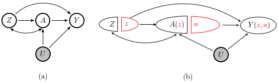
Figure 1: (a) Causal Directed Acyclic Graph (Pearl, 2009) representing the invalid IV model within strata of measured baseline covariates, with a bi-directed arrow between $Z$ and $A$ indicating potential unmeasured common causes of $Z$ and $A$. (b) The corresponding Single World Intervention Graph (Richardson and Robins, 2013) with a bi-directed arrow.

The ATE in the overall population $E\{Y(1)-Y(0)\}$ is arguably the causal parameter of interest in many studies for policy questions (Robins and Greenland, 1996; Imbens, 2010), but it cannot be identified under Assumptions 1 and 2 without further restrictions. Much of the invalid IV literature considered structural assumptions primarily in multiple-IV settings $Z=(Z_{1},Z_{2},...,Z_{p})^{\mathrm{\scriptscriptstyle T}}$ which imply the joint semiparametric partially linear model

$$\begin{split}E(Y|A,Z,X,U)&=\boldsymbol{\theta}^{\mathrm{\scriptscriptstyle T}}_{1}Z+\beta A+\xi_{y}(X,U);\\ E(A|Z,X,U)&=\boldsymbol{\theta}^{\mathrm{\scriptscriptstyle T}}_{2}Z+\xi_{a}(X,U),\end{split}$$ (3)

indexed by the parameters $\beta\in{\rm I\!R},\boldsymbol{\theta}_{1}=(\theta_{11},...,\theta_{1p})^{\mathrm{\scriptscriptstyle T}}\in{\rm I\!R}^{p},\boldsymbol{\theta}_{2}=(\theta_{21},...,\theta_{2p})^{\mathrm{\scriptscriptstyle T}}\in{\rm I\!R}^{p}$, and the confounding effects of the measured and unmeasured confounders on the outcome and treatment are respectively encoded by the measurable and square integrable $\xi_{y}(\cdot)$ and $\xi_{a}(\cdot)$, which remain unspecified. Under the multivariate-IV version of Assumption 1 and correct specification of the partially linear model (3), the scalar parameter $\beta$ equals the population ATE. The parameter $\boldsymbol{\theta}_{1}$ represents direct effects of $Z$ on $Y$. Identification of $\beta$ (or equivalently the ATE) under (1)–(3) when $\theta_{1j}\neq 0$ for some $j\in\mathcal{J}\subseteq\{1,2,...,p\}$ has been an area of active research, generally by imposing additional restrictions on the nuisance parameter space of $\{\boldsymbol{\theta}_{1},\boldsymbol{\theta}_{2}\}$ (Kolesár et al., 2015; Bowden et al., 2016; Kang et al., 2016; Windmeijer et al., 2019; Guo et al., 2018).

2.1 Nonparametric identification without exclusion restriction

In this paper, we consider the following generalization of (3).

Assumption 3

$$\begin{split}E(Y|A,Z,X,U)&=\theta_{1}(X)Z+\beta(X)A+\xi_{y}(X,U);\\ E(A|Z,X,U)&=\theta_{2}(X)Z+\xi_{a}(X,U),\end{split}$$ (4)

where $\{\beta(\cdot),\theta_{1}(\cdot),\theta_{2}(\cdot)\}$ are unknown measurable and square integrable scalar functions of the measured covariates.

Following the tradition in the IV literature (Robins, 1994; Imbens and Angrist, 1994; Angrist et al., 1996; Heckman, 1997), we focus on the canonical case of binary $A$ and $Z$; the framework can be extended readily to categorical $A$ and $Z$. The structural equation (4) models the marginal effect of each scalar $Z$ on the outcome and the treatment which can vary with the value of observed covariates, rather than the joint effects of all available IVs, and therefore represents a significant relaxation of the restrictions in (3). We follow the latent IV formulation of Swanson et al. (2018) and formally define the no direct effect assumption or exclusion restriction as

$$E\{Y(z,a)|X,U\}=E\{Y(z^{\prime},a)|X,U\}\text{ for all }z,z^{\prime},a\in\{0,1\},$$

which explicitly incorporates the unmeasured confounder $U$ (Dawid, 2003; Didelez et al., 2010). Under Assumptions 1 and 2, $E\{Y(z,a)|X,U\}=E\{Y(z,a)|A=a,Z=z,X,U\}=E\{Y|A=a,Z=z,X,U\}$. Therefore $\theta_{1}(X)=E\{Y(1,a)|X,U\}-E\{Y(0,a)|X,U\}$ encodes the population average direct effect on the outcome within levels of $(X,U)$ for a change of the IV’s value from $0$ to $1$ at each treatment level; exclusion restriction is violated in model (4) if $\theta_{1}(X)\neq 0$ for at least one value in the support of $X$. In addition, under Assumption 1 and consistency, $E\{Y(1)-Y(0)|Z,X,U\}=E\{Y(1)|A=1,Z,X,U\}-E\{Y(0)|A=0,Z,X,U\}=E\{Y|A=1,Z,X,U\}-E\{Y|A=0,Z,X,U\}=\beta(X)$ equals the conditional ATE within levels of $(Z,X,U)$.

A design implication of (4) is that even when $Z$ is randomized, it remains important to measure as many effect modifiers in the outcome and treatment models as possible in the hope that no residual effect modification involving $U$ remains within strata of the measured covariates $X$. We show in the Appendix that (4) may be relaxed so that $\{\beta(\cdot),\theta_{1}(\cdot),\theta_{2}(\cdot)\}$ varies with $U$ (albeit in restricted ways) even after controlling for $X$, a setting also known as essential heterogeneity in the IV literature (Heckman et al., 2006). Essential heterogeneity is more realistic in a variety of settings. For example, the choice of medical treatment is likely influenced by idiosyncratic gains from alternative treatment in the analysis of health-care decisions. The direct effect of treatment assignment on the outcome may also be influenced by knowledge of such gains if double-blinding is either absent or compromised in randomized studies (Ten Have et al., 2008). For these reasons, we focus on (4) for identification and inference, although an alternative identification approach involving the nonlinear multiplicative model

$$\log\{p_{1}(X,U)/p_{0}(X,U)\}=\tilde{\theta}_{2}(X),$$

where $p_{z}(X,U):=P(A=1|Z=z,X,U)$, may be used for binary treatment which rules out essential heterogeneity (Tchetgen Tchetgen et al., 2021). As pointed out by the reviewers, the function ${\theta}_{2}(X)$ cannot in general be variation independent of the function $\xi_{a}(X,U)$ if the resulting treatment conditional mean $E(A|Z,X,U)$ must remain in the unit interval. Nevertheless, a variation independent parameterization of $E(A|Z,X,U)$ is possible such that the aforementioned dependence can be encoded in a manner compatible with our identifying assumptions, by using the odds product parameterization of Richardson et al. (2017) detailed in Appendix B which is compatible with natural constraints of the data generating mechanism.

Let $\beta_{0}(x)$, $\mu_{0}(z,x):=P(A=1|Z=z,X=x)$ and $\varepsilon:=A-\mu_{0}(Z,X)$ denote the true conditional ATE function, treatment propensity score and the treatment regression residual respectively. In what follows the residual $\varepsilon$ serves to tease out the treatment effect via its orthogonality to direct effect component $\theta_{1}(X)Z$. We show in the Appendix that under Assumptions 2 and 3,

$$E(\varepsilon Y|Z,X)=\beta_{0}(X)\text{Var}(A|Z,X)+\rho_{0}(X),$$ (5)

where $\text{Var}(A|Z=z,X=x):=\mu_{0}(z,x)\{1-\mu_{0}(z,x)\}$ denotes the conditional variance of $A$ within the subpopulation $\{Z=x,X=x\}$ and $\rho_{0}(x):=E\{\varepsilon(Y-\beta_{0}(X)A)|X=x\}$. The conditional covariance independence restriction

$$E\{\varepsilon(Y-\beta_{0}(X)A)|Z,X\}=\text{Cov}\{\xi_{a}(X,U),\xi_{y}(X,U)|Z,X\}=\rho_{0}(X),$$

holds almost surely under Assumptions 2 and 3. Therefore the function $\rho_{0}(\cdot)$ may be interpreted as encoding the degree of stratum-specific unmeasured confounding. Additional regularity conditions on the observed data law are required for identification of the ATE.

Assumption 4

The true observed data distribution lies in the interior of the nonparametric model $\mathcal{M}$ that satisfies $\text{Var}(A|Z=1,X)-\text{Var}(A|Z=0,X)\neq 0$ (heteroscedasticity), and $\pi_{0}(1|X):=P(Z=1|X)\in(c,1-c)$ for some $c\in(0,1/2)$ (positivity), almost surely.

Assumption 4 consists of observed data restrictions that are empirically testable. Heteroscedasticity has been widely used in prior works as a source of identification in linear structural models without exclusion restrictions (Rigobon, 2003; Klein and Vella, 2010; Lewbel, 2012) and represents a strengthening of the traditional IV relevance assumption $P(A=1|Z=1,X)-P(A=1|Z=0,X)\neq 0$ in the context of binary $A$ and $Z$, as it further requires $P(A=1|Z=1,X)+P(A=1|Z=0,X)\neq 1$ to hold almost surely. Positivity ensures that there is overlap in the distribution of baseline covariates $X$ among $Z=0$ and $Z=1$ units so that the treatment effect within each level of $X$ can be identified. Equation (5) in conjunction with Assumptions 1 and 4 implies that

$$\begin{gathered}\text{ATE}=E\{\beta_{0}(X)\}=E\left\{\frac{E(\varepsilon Y|Z=1,X)-E(\varepsilon Y|Z=0,X)}{\text{Var}(A|Z=1,X)-\text{Var}(A|Z=0,X)}\right\}.\end{gathered}$$ (6)

The nonparametric representation in (6) appears to be new in literature and has a form similar to the well-known Wald estimand as a ratio of differences between the two instrument groups. Similar to the Wald estimand, estimation based on (6) may be vulnerable to bias and large variance if $\text{Var}(A|Z,X)$ only weakly depends on $Z$. In recent work, Ye et al. (2021) proposed a measure of weak identification relative to sample size and developed inference under a many weak invalid IVs asymptotic regime, which however requires correct specification of parametric models for all nuisance parameters. The observed data density $P(O)$ with respect to some appropriate dominating measure factorizes as $P(Y,A|Z,X)\times P(Z|X)\times P(X)$. Evaluation of (6) requires knowledge of the joint density $P(Y,A|Z,X)$. As will be shown below, identification of the ATE may be established based on some but not necessarily all of these factors. We introduce the additional notation $\tau_{0}(z,x):=E\{Y-\beta_{0}(X)A|Z=z,X=x\}$ to simplify presentation for this purpose.

Theorem 1

Under Assumptions 1–4, the ATE $\gamma:=E\{Y(1)-Y(0)\}=E\{\beta_{0}(X)\}$ is identified in $\mathcal{M}$ through the following three representations, each of which involves a distinct set of nuisance parameters:

Explicit representation (i):

$0=E\{\varphi_{1}(O;\pi_{0},\mu_{0})|X\}-\beta_{0}(X)$ almost surely, where

$$\begin{gathered}\varphi_{1}(O;\pi_{0},\mu_{0}):=\frac{(2Z-1)\varepsilon Y}{\pi_{0}(Z|X)(\text{Var}(A|Z=1,X)-\text{Var}(A|Z=0,X))};\end{gathered}$$ (7)

Implicit representation (ii):

$0=E\{\varphi_{2}(O;\pi_{0},\beta_{0},\tau_{0})|X\}$ almost surely, where

$$\begin{gathered}\varphi_{2}(O;\pi_{0},\beta_{0},\tau_{0}):=\frac{(2Z-1)A\{Y-\beta_{0}(X)A-\tau_{0}(Z,X)\}}{\pi_{0}(Z|X)};\end{gathered}$$ (8)

Implicit representation (iii):

$0=E\{\varphi_{3}(O;\mu_{0},\beta_{0},\rho_{0})|Z,X\}$ almost surely, where

$$\begin{gathered}\varphi_{3}(O;\mu_{0},\beta_{0},\rho_{0}):=\varepsilon\{Y-\beta_{0}(X)A\}-\rho_{0}(X).\end{gathered}$$ (9)

In particular, representation (i) provides a generalization of the results in Lewbel (2012) and Tchetgen Tchetgen et al. (2021) which both rely on a priori restrictions on the functional form of the conditional treatment effect within strata of measured covariates,

$$E\left\{\varphi_{1}(O;\pi_{0},\mu_{0})\rvert X=x\right\}=\frac{\text{Cov}\{Z,\varepsilon Y|X=x\}}{\text{Cov}\{Z,\varepsilon A|X=x\}}=\beta(x;\eta),$$

where $\eta$ is a finite-dimensional parameter. G-estimators developed in the context of additive and multiplicative structural mean models (Robins, 1989, 1994) may be constructed based on unconditional forms of the equivalent restriction

$$\text{Cov}\{Z,\varepsilon(Y-\beta(X;\eta)A)|X=x\}=0.$$ (10)

No such restriction is needed in representation (i). Thus in principle we can construct the plug-in estimator $\hat{\gamma}=\mathbb{P}_{n}\{\varphi_{1}(O;\hat{\pi},\hat{\mu})\}$, where $\mathbb{P}_{n}$ denotes the empirical mean operator $\mathbb{P}_{n}\{G(O)\}=n^{-1}\sum_{i}G(O_{i})$ and $(\hat{\pi},\hat{\mu})$ are nonparametric first-step estimators of $(\pi_{0},\mu_{0})$ which consists of conditional mean functions. Because we are not restricting $\mathcal{M}$ except for regularity conditions, nonparametric estimators of $\gamma$ based on representations (i)–(iii) are in fact asymptotically equivalent with common influence function given in the following Theorem 2.

Theorem 2

The efficient influence function for estimating $\gamma$ in $\mathcal{M}$ is given by

$$\varphi_{\textup{eff}}(O;\pi_{0},\mu_{0},\beta_{0},\tau_{0},\rho_{0})-\gamma,$$

where

$$\varphi_{\textup{eff}}(O;\pi,\mu,\beta,\tau,\rho) =\frac{(2Z-1)\left\{\varepsilon(Y-\beta(X)A-\tau(Z,X))-\rho(X)\right\}}{\pi(Z|X)\{\text{Var}(A|Z=1,X)-\text{Var}(A|Z=0,X)\}}+\beta\left(X\right).$$

Therefore, the semiparametric efficiency bound for estimating $\gamma$ in $\mathcal{M}$ is

$$E\{(\varphi_{\textup{eff}}(O;\pi_{0},\mu_{0},\beta_{0},\tau_{0},\rho_{0})-\gamma)^{2}\}.$$

In most practical settings, we anticipate that $X$ will generally be of moderate to high dimension relative to the sample size, as analysts consider a broad collection of covariates and their functional forms in the hope of capturing the salient features of the confounding effects. In this case, nonparametric estimators of $\gamma$ may exhibit poor finite-sample behavior due to the curse of dimensionality (Robins and Ritov, 1997). Below, we describe two distinct strategies for modeling the nuisance parameters: the first uses standard parametric models, while the second leverages modern machine learning.

3 Multiply robust estimation

Consider the working parametric models $\{\pi(z|x;\eta_{1}),\mu(z,x;\eta_{2}),\beta(x;\eta_{3}),\tau(z,x;\eta_{4}),\rho(x;\eta_{5})\}$ indexed by finite-dimensional parameters $\eta=(\eta^{\mathrm{\scriptscriptstyle T}}_{1},\eta^{\mathrm{\scriptscriptstyle T}}_{2},\eta^{\mathrm{\scriptscriptstyle T}}_{3},\eta^{\mathrm{\scriptscriptstyle T}}_{4},\eta^{\mathrm{\scriptscriptstyle T}}_{5})^{\mathrm{\scriptscriptstyle T}}$. A two-step procedure to estimate the nuisance parameters is as follows:

Procedure 1.
(i) Solve the score equation $0=\mathbb{P}_{n}\{S(A,Z,X;\eta_{1},\eta_{2})\}$ to obtain $(\hat{\eta}^{\mathrm{\scriptscriptstyle T}}_{1},\hat{\eta}^{\mathrm{\scriptscriptstyle T}}_{2})^{\mathrm{\scriptscriptstyle T}}$, where

$$S(A,Z,X;\eta_{1},\eta_{2})=\frac{\partial\log P(A,Z|X;\eta_{1},\eta_{2})}{\partial({\eta}^{\mathrm{\scriptscriptstyle T}}_{1},{\eta}^{\mathrm{\scriptscriptstyle T}}_{2})^{\mathrm{\scriptscriptstyle T}}}.$$

(ii) Solve $0=\mathbb{P}_{n}\{G(O;\hat{\eta}_{1},\hat{\eta}_{2},\eta_{3},\eta_{4},\eta_{5})\}$ to obtain $(\hat{\eta}^{\mathrm{\scriptscriptstyle T}}_{3},\hat{\eta}^{\mathrm{\scriptscriptstyle T}}_{4},\hat{\eta}^{\mathrm{\scriptscriptstyle T}}_{5})^{\mathrm{\scriptscriptstyle T}}$, where

$$G(O;\eta):=\left[\begin{array}[]{c}D_{3}(X)\frac{2Z-1}{\pi(Z|X;\eta_{1})}\{\varepsilon(\eta_{2})(Y-\beta(X;\eta_{3})A-\tau(Z,X;\eta_{4}))-\rho(X;\eta_{5})\}\\ D_{4}(X)\{Y-\beta(X;\eta_{3})A-\tau(Z,X;\eta_{4})\}\\ D_{5}(X)\{\varepsilon(\eta_{2})(Y-\beta(X;\eta_{3})A)-\rho(X;\eta_{5})\}\end{array}\right],$$

and $D_{j}(X)$ is a user-specified vector function of the same dimension as $\eta_{j}$ for $j=3,4,5$.

Similar to Bang and Robins (2005); Tchetgen Tchetgen et al. (2009); Sun et al. (2018); Sun and Tchetgen Tchetgen (2018); Wang and Tchetgen Tchetgen (2018), in the following we propose the estimator $\hat{\gamma}_{mr}=\mathbb{P}_{n}\{\varphi_{\text{eff}}(O;\hat{\pi},\hat{\mu},\hat{\beta},\hat{\tau},\hat{\rho})\}$ based on the form of the efficient influence function given in Theorem 2, where $\hat{\pi}=\pi(\cdot;\hat{\eta}_{1})$, $\hat{\mu}=\mu(\cdot;\hat{\eta}_{2})$, $\hat{\beta}=\beta(\cdot;\hat{\eta}_{3})$, $\hat{\tau}=\tau(\cdot;\hat{\eta}_{4})$ and $\hat{\rho}=\rho(\cdot;\hat{\eta}_{5})$. Let $\eta^{\ast}$ denote the probability limit of $\hat{\eta}$. Because the two-step estimator $\hat{\eta}$ may be viewed as solving the joint moment equation $0=\mathbb{P}_{n}\{\tilde{G}(O;\eta)\}$ where $\tilde{G}(O;\gamma)=\{S^{\mathrm{\scriptscriptstyle T}}(A,Z,X;\eta_{1},\eta_{2}),G^{\mathrm{\scriptscriptstyle T}}(O;\eta)\}^{\mathrm{\scriptscriptstyle T}}$ (Newey and McFadden, 1994), the following result holds by invoking the $n^{-1/2}$ asymptotic expansion for $\hat{\eta}-\eta^{\ast}$, allowing for model misspecification (White, 1982).

Lemma 1

Under standard regularity conditions for method of moments estimation (Newey and McFadden, 1994), $\eta^{\ast}$ is the unique solution to $E\{\tilde{G}(O;\eta)\}=0$. Furthermore, $\hat{\gamma}_{mr}$ is a consistent and asymptotically normal (CAN) estimator of ${\gamma}^{\ast}_{mr}=E\{\varphi_{\textup{eff}}(O;\eta^{\ast})\}$,

$$\sqrt{n}(\hat{\gamma}_{mr}-{\gamma}^{\ast}_{mr})\xrightarrow[]{d}N(0,\Sigma),$$

where $\Sigma=E[\{\varphi_{mr}(O;\eta^{\ast})-{\gamma}^{\ast}_{mr}\}^{2}]$ and

$$\varphi_{mr}(O;\eta^{\ast})=\varphi_{\textup{eff}}(O;{\eta}^{\ast})-E\left\{\frac{\partial\varphi_{\textup{eff}}(O;\eta)}{\partial\eta^{\mathrm{\scriptscriptstyle T}}}\biggr{\rvert}_{\eta=\eta^{\ast}}\right\}\times\left[E\left\{\frac{\partial\tilde{G}(O;\eta)}{\partial\eta}\biggr{\rvert}_{\eta=\eta^{\ast}}\right\}\right]^{-1}\tilde{G}(O;\eta^{\ast}).$$

Let ${\pi}^{\ast}=\pi(\cdot;{\eta}^{\ast}_{1})$, ${\mu}^{\ast}=\mu(\cdot;{\eta}^{\ast}_{2})$, ${\beta}^{\ast}=\beta(\cdot;{\eta}^{\ast}_{3})$, ${\tau}^{\ast}=\tau(\cdot;{\eta}^{\ast}_{4})$ and ${\rho}^{\ast}=\rho(\cdot;{\eta}^{\ast}_{5})$ denote the probability limits under the (possibly misspecified) working models. Based on the three distinct sets of nuisance parameters characterized in Theorem 1, the efficient influence function has the multiple robustness property that $\gamma=E\{\varphi_{\text{eff}}(O;{\pi}^{\ast},{\mu}^{\ast},{\beta}^{\ast},{\tau}^{\ast},{\rho}^{\ast})\}$ if at least one of the following holds: (i) $({\pi}^{\ast},{\mu}^{\ast})=(\pi_{0},\mu_{0})$; (ii) $({\pi}^{\ast},{\beta}^{\ast},{\tau}^{\ast})=(\pi_{0},\beta_{0},\tau_{0})$ and (iii) $({\mu}^{\ast},{\beta}^{\ast},{\rho}^{\ast})=(\mu_{0},\beta_{0},\rho_{0})$. This suggests that $\hat{\gamma}_{mr}$ is a CAN estimator of $\gamma$ under one, but not necessarily more than one, of the following three different sets of model assumptions:

$\mathcal{M}_{1}$:

models for $(\pi_{0},\mu_{0})$ are correctly specified;

$\mathcal{M}_{2}$:

models for $(\pi_{0},\beta_{0},\tau_{0})$ are correctly specified;

$\mathcal{M}_{3}$:

models for $(\mu_{0},\beta_{0},\rho_{0})$ are correctly specified.

Lemma 2

$\hat{\gamma}_{mr}$ is a CAN estimator of $\gamma$ in the union model $\mathcal{M}_{{{union}}}=\cup_{k=1}^{3}\mathcal{M}_{k}$. Furthermore, $\hat{\gamma}_{mr}$ attains the semiparametric efficiency bound in $\mathcal{M}$ at the intersection submodel $\cap_{k=1}^{3}\mathcal{M}_{k}$ where all the working models are correctly specified.

Following a theorem due to Robins and Rotnitzky (2001), $\hat{\gamma}_{mr}$ can be shown to also attain the semiparametric efficiency bound for $\mathcal{M}_{{{union}}}$ at the intersection submodel $\cap_{k=1}^{3}\mathcal{M}_{k}$. Because the nuisance parameters in each of $\mathcal{M}_{1}$, $\mathcal{M}_{2}$ and $\mathcal{M}_{3}$ are variation independent of each other, multiply robust estimation gives the analyst three genuine opportunities to obtain valid inferences about $\gamma$, even under partial misspecification of the observed data models.

3.1 Comparison with existing estimators

Under the particular specification $\{\beta(x;\eta_{3}),\tau(z,x;\eta_{4}),\rho(x;\eta_{5})\}=\{0,0,0\}$, $\hat{\gamma}_{mr}$ reduces to the semiparametric plug-in estimator $\hat{\gamma}_{1}=\mathbb{P}_{n}\{\varphi_{1}(O;\hat{\pi},\hat{\mu})\}$ which is CAN only in $\mathcal{M}_{1}$. An appealing feature of $\hat{\gamma}_{1}$ is that the nuisance parameters can all be estimated in step (i) of procedure 1 without involving outcome data, and therefore mitigates potential for “data-dredging” exercises (Rubin, 2007). However, $\hat{\gamma}_{1}$ is neither multiply robust nor locally efficient. Furthermore, $\hat{\gamma}_{mr}$ is expected to be more efficient than $\hat{\gamma}_{1}$, since the latter fails to incorporate information from $(A,Z,X)$ which may be predictive of the outcome values. Such efficiency considerations are analogous to related results on covariate adjustment in completely randomized experiments with full compliance (Leon et al., 2003; Davidian et al., 2005; Rubin and van der Laan, 2011).

Based on moment condition (13), Tchetgen Tchetgen et al. (2021) proposed the covariate-adjusted “Mendelian Randomization G-Estimation under No Interaction with Unmeasured Selection” (MR GENIUS) estimator $\hat{\eta}^{g}_{3}$ which solves

$$0=\mathbb{P}_{n}\left\{\frac{D_{3}(X)(2Z-1)\varepsilon(\hat{\eta}_{2})(Y-\beta(X;\eta_{3})A)}{\pi(Z|X;\hat{\eta}_{1})}\right\}.$$ (12)

It is straightforward to verify that $\hat{\gamma}_{g}=\mathbb{P}_{n}\{\beta(X;\hat{\eta}_{3}^{g})\}$ is a CAN estimator of $\gamma$ under the model assumption

$\mathcal{M}_{1}^{\prime}$:

models for $(\pi_{0},\mu_{0},\beta_{0})$ are correct.

Interestingly, under Assumptions 1–3 and no unmeasured confounding given $(Z,X)$, i.e., if either $U\rotatebox[origin={c}]{90.0}{$\models$}A|Z,X$ or $U\rotatebox[origin={c}]{90.0}{$\models$}Y|A,Z,X$, the G-estimator $\hat{\eta}_{3}$ of Robins (1989, 1994) solves

$$0=\mathbb{P}_{n}\left\{D_{3}(X)\varepsilon(\hat{\eta}_{2})(Y-\beta(X;\eta_{3})A)\right\},$$ (13)

and $\hat{\gamma}=\mathbb{P}_{n}\{\beta(X;\hat{\eta}_{3})\}$ is a CAN estimator of $\gamma$. Similar to standard G-estimation, a more efficient MR GENIUS estimator $\tilde{\eta}^{g}_{3}$ may be obtained as the joint solution to

$$0=\mathbb{P}_{n}\left\{\begin{array}[]{c}\frac{D_{3}(X)(2Z-1)\varepsilon(\hat{\eta}_{2})(Y-\beta(X;\eta_{3})A-\tau(Z,X;\eta_{4}))}{\pi(Z|X;\hat{\eta}_{1})}\\ D_{4}(X)(Y-\beta(X;\eta_{3})A-\tau(Z,X;\eta_{4}))\\ \end{array}\right\},$$ (16)

where information about the association between $(Z,X)$ and $Y$ is incorporated via an additional working model for $\tau_{0}(\cdot)$. Lewbel (2012) considered semiparametric estimation based on moment restrictions similar to (16) but with nonparametric plug-ins for the nuisance parameters $(\eta_{1},\eta_{2})$. The resulting estimator $\tilde{\gamma}_{g}=\mathbb{P}_{n}\{\beta(X;\tilde{\eta}^{g}_{3})\}$ is doubly robust in the union model ${\mathcal{M}}^{\prime}_{1}\cup{\mathcal{M}}_{2}$, which is in turn a submodel of $\mathcal{M}_{{{union}}}$.

4 Flexible estimation of nuisance parameters

With high-dimensional $X$, various flexible and data-adaptive statistical or machine learning methods may be adopted to estimate the nuisance parameters $\eta_{0}=(\pi_{0},\mu_{0},\beta_{0},\tau_{0},\rho_{0})$, including random forests, Lasso, neural nets, boosting or their ensembles. Recent work by Chernozhukov et al. (2018, 2022) show that $\surd{n}$-consistent estimation of $\gamma$ is possible even when the complexity of the nuisance parameters is not tractable by standard empirical process theory (e.g. Vapnik-Chervonenkis and Donsker classes). Let $({I}_{k})_{k=1}^{K}$ be a $K$-fold random partition of the observation indices $\{1,2,...,n\}$. For each $k$, let $\hat{\pi}(k)$, $\hat{\mu}(k)$, $\hat{\beta}(k)$, $\hat{\tau}(k)$ and $\hat{\rho}(k)$ be learners of the nuisance parameters that are constructed using all observations not in $I_{k}$ based on the following two-step procedure.

Procedure 2.
(i) Obtain $\hat{\pi}(k)$ and $\hat{\mu}(k)$ by machine learning of the conditional mean functions $({\pi}_{0},{\mu}_{0})$.
(ii) Given $\hat{\pi}(k)$ and $\hat{\mu}(k)$, obtain $\hat{\beta}(k)$, $\hat{\tau}(k)$ and $\hat{\rho}(k)$ sequentially by machine learning based on the following conditional mean relationships: ${\beta}(x;\pi,\mu)=E\left\{\varphi_{1}(O;\pi,\mu)\rvert X=x\right\}$, $\tau(z,x;\beta)=E\{{Y}-\beta(X)A\rvert Z=z,X=x\}$ and $\rho(x;\mu,\beta)=E\{\varepsilon(\mu)({Y}-\beta(X)A)\rvert X=x\}$.

The cross-fitted debiased machine learning (DML) estimator of $\gamma$ is

$$\hat{\gamma}_{dml}=\frac{1}{n}\sum^{K}_{k=1}\sum_{i\in I_{k}}\varphi_{\text{eff}}(O_{i};\hat{\pi}(k),\hat{\mu}(k),\hat{\beta}(k),\hat{\tau}(k),\hat{\rho}(k)).$$

By definition, the efficient influence function $\varphi_{\text{eff}}(O;\eta)$ satisfies the Neyman orthogonality condition (Neyman, 1959, 1979; Belloni et al., 2017; Chernozhukov et al., 2018, 2022), as all first order influence functions admit second order bias (Robins et al., 2009). Under general regularity conditions established by Chernozhukov et al. (2018, 2022), $\hat{\gamma}_{dml}$ is CAN if all the nuisance parameters are estimated with mean-squared error rates diminishing faster than $n^{-1/4}$. Such rates are achievable for many highly data-adaptive machine learning methods, including LASSO (Tibshirani, 1996), gradient boosting trees (Friedman, 2001), random forests (Breiman, 2001; Wager and Athey, 2018) or ensembles of these methods. We note that in low-dimensional settings, Lemma 2 shows that $\hat{\gamma}_{mr}$ is CAN even when some of the nuisance models is misspecified by invoking the usual $n^{-1/2}$ asymptotic expansion (White, 1982), which is not applicable when nuisance parameters are estimated via machine learning methods. Therefore while methods such as DML and CV-TMLE (Zheng and Van Der Laan, 2010; Van der Laan and Rose, 2011) with machine learning remain consistent when various strict subsets of nuisance parameter learners (e.g. $\hat{\pi}$ and $\hat{\mu}$) are consistent due to the multiple robustness property of the efficient influence function $\varphi_{\text{eff}}(O;\eta)$, they generally require consistent estimation of all nuisance parameters in order to obtain valid confidence intervals.

4.1 Selective machine learning of multiply robust functionals

The performance of DML estimators is intimately related to the choice of the nuisance parameter learners, even when the latter includes flexible machine learning or other nonparametric data adaptive methods. For this reason, generally one would like to learn adaptively from data and avoid choosing models ex ante. The task of model selection of parametric nuisance models was recently considered by Han and Wang (2013), Chan (2013), Han (2014), Chan et al. (2014), Duan and Yin (2017), Chen and Haziza (2017) and Li et al. (2020) in specific semiparametric doubly robust estimation settings. A related strand of work is CV-TMLE which can provide notable improvements by incorporating an ensemble of semiparametric or nonparametric methods. Nonetheless, the above methods primarily focused on optimal estimation of nuisance parameters, but not bias reduction of the functional ultimately of interest. This latter task is considerably more challenging since the risk of a nonparametric functional does not typically admit an unbiased estimator and therefore may not be minimized without excessive error. Cui and Tchetgen Tchetgen (2021) proposed a novel model selection criteria for bias reduction in estimating nonparametric functionals of interest, based on minimization of a cross-validated empirical quadratic pseudo-risk in the context of doubly robust estimating functions. In this paper we propose to extend their work to the multiply robust setting.

Consider the collection of candidate parametric or nonparametric learners

$$\mathcal{L}=\{\hat{\eta}{(\alpha)}=\hat{\eta}{(\alpha_{1},\alpha_{2},\alpha_{3},\alpha_{4},\alpha_{5})}=(\hat{\pi}_{\alpha_{1}},\hat{\mu}_{\alpha_{2}},\hat{\beta}_{\alpha_{3}},\hat{\tau}_{\alpha_{4}},\hat{\rho}_{\alpha_{5}}):1\leq\alpha_{j}\leq r_{j}\text{ for }j=1,...,5\},$$

with probability limits $\{{\eta}{(\alpha)}={\eta}{(\alpha_{1},\alpha_{2},\alpha_{3},\alpha_{4},\alpha_{5})}:1\leq\alpha_{j}\leq r_{j}\text{ for }j=1,...,5\}$. Suppose one of the candidate learners $\hat{\eta}{(\check{\alpha})}\in\mathcal{L}$ is consistent so that ${\eta}{(\check{\alpha})}=(\pi_{0},\mu_{0},\beta_{0},\tau_{0},\rho_{0})$. The proposed procedure relies crucially on the following two sets of mean zero implications due to the multiply robust property of the efficient influence function, that for all $1\leq\alpha_{j}\leq r_{j}$, $1\leq{\alpha}^{\prime}_{j}\leq r_{j}$, $j\in\{1,...,5\}$,

$$0 =E\{\bar{\varphi}_{\text{eff}}(\check{\alpha}_{1},\check{\alpha}_{2},\check{\alpha}_{3},\check{\alpha}_{4},\check{\alpha}_{5})-\bar{\varphi}_{\text{eff}}(\check{\alpha}_{1},\check{\alpha}_{2},\alpha_{3},\alpha_{4},\alpha_{5})\};$$ (17)

$$0 =E\{\bar{\varphi}_{\text{eff}}(\check{\alpha}_{1},\check{\alpha}_{2},\check{\alpha}_{3},\check{\alpha}_{4},\check{\alpha}_{5})-\bar{\varphi}_{\text{eff}}(\check{\alpha}_{1},\alpha_{2},\check{\alpha}_{3},\check{\alpha}_{4},\alpha_{5})\};$$

$$0 =E\{\bar{\varphi}_{\text{eff}}(\check{\alpha}_{1},\check{\alpha}_{2},\check{\alpha}_{3},\check{\alpha}_{4},\check{\alpha}_{5})-\bar{\varphi}_{\text{eff}}(\alpha_{1},\check{\alpha}_{2},\check{\alpha}_{3},\alpha_{4},\check{\alpha}_{5})\},$$

and

$$0 =E\{\bar{\varphi}_{\text{eff}}(\check{\alpha}_{1},\check{\alpha}_{2},{\alpha}^{\prime}_{3},{\alpha}^{\prime}_{4},{\alpha}^{\prime}_{5})-\bar{\varphi}_{\text{eff}}(\check{\alpha}_{1},\check{\alpha}_{2},\alpha_{3},\alpha_{4},\alpha_{5})\};$$ (18)

$$0 =E\{\bar{\varphi}_{\text{eff}}(\check{\alpha}_{1},{\alpha}^{\prime}_{2},\check{\alpha}_{3},\check{\alpha}_{4},{\alpha}^{\prime}_{5})-\bar{\varphi}_{\text{eff}}(\check{\alpha}_{1},\alpha_{2},\check{\alpha}_{3},\check{\alpha}_{4},\alpha_{5})\};$$

$$0 =E\{\bar{\varphi}_{\text{eff}}({\alpha}^{\prime}_{1},\check{\alpha}_{2},\check{\alpha}_{3},{\alpha}^{\prime}_{4},\check{\alpha}_{5})-\bar{\varphi}_{\text{eff}}(\alpha_{1},\check{\alpha}_{2},\check{\alpha}_{3},\alpha_{4},\check{\alpha}_{5})\},$$

where $\bar{\varphi}_{\text{eff}}(\alpha):=\varphi_{\text{eff}}(O;\eta(\alpha))$. To ease presentation, we introduce the sets $\mathscr{C}=\{1,2,3,4,5\}$, $\mathscr{C}_{1}=\{3,4,5\}$, $\mathscr{C}_{2}=\{2,5\}$ and $\mathscr{C}_{3}=\{1,4\}$ which index the nuisance learner components. Let $\alpha_{+k}$ denote the counters for the nuisance learner components indexed by the elements in $\mathscr{C}_{k}$, e.g. $\alpha_{+1}=(\alpha_{3},\alpha_{4},\alpha_{5})$. Similarly, let $\alpha_{-k}$ denote the counters for the nuisance learner components indexed by the elements in $\mathscr{C}$ but not in $\mathscr{C}_{k}$, e.g. $\alpha_{-1}=(\alpha_{1},\alpha_{2})$. Then (17) and (18) may be restated more concisely as

$$0=E\{\bar{\varphi}_{\text{eff}}(\check{\alpha}_{-k},\check{\alpha}_{+k})-\bar{\varphi}_{\text{eff}}(\check{\alpha}_{-k},\alpha_{+k})\},$$ (19)

and

$$0=E\{\bar{\varphi}_{\text{eff}}(\check{\alpha}_{-k},{\alpha}_{+k})-\bar{\varphi}_{\text{eff}}(\check{\alpha}_{-k},\alpha^{\prime}_{+k})\},$$ (20)

respectively, for all ${\alpha}_{+k}$, $\alpha^{\prime}_{+k}\in\mathscr{A}_{k}:=\{\alpha_{+k}:1\leq{\alpha}_{j}\leq r_{j},j\in\mathscr{C}_{k}\}$, $k\in\{1,2,3\}$. These mean zero conditions suggest perturbing the learners indexed by $\alpha_{+k}$ and using some measure of the resulting spread as a basis for selecting between the learners indexed by $\alpha_{-k}$. Towards this end we introduce two different norms to define the spread or pseudo-risk. The first type is given by the overall maximum squared bias (i.e., change in the estimated functional) induced by perturbing one distinct set of learners at a time while holding the remaining ones fixed. For an arbitrary learner $\hat{\eta}{(\alpha^{\ast})}\in\mathcal{L}$, we define the minimax pseudo-risk $\mathcal{R}^{(1)}(\alpha^{\ast})=\max_{k\in\{1,2,3\}}\Lambda^{(1)}_{k}(\alpha),$ where

$$\Lambda^{(1)}_{k}({\alpha^{\ast}})=\max_{\begin{subarray}{c}\alpha_{+k}\in\mathscr{A}_{k}\end{subarray}}[E\{\bar{\varphi}_{\text{eff}}(\alpha^{\ast}_{-k},\alpha^{\ast}_{+k})-\bar{\varphi}_{\text{eff}}(\alpha^{\ast}_{-k},\alpha_{+k})\}]^{2},\text{ for }k=1,2,3.$$

The second type is given by the sum of three maximum squared bias terms, each capturing the bias induced by perturbing a distinct set of learners. We define the mixed minimax pseudo-risk $\mathcal{R}^{(2)}(\alpha^{\ast})=\sum_{k=1}^{3}\Lambda^{(2)}_{k}(\alpha^{\ast}),$ where

$$\Lambda^{(2)}_{k}({\alpha^{\ast}})=\max_{\begin{subarray}{c}\alpha_{+k},\alpha^{\prime}_{+k}\in\mathscr{A}_{k}\end{subarray}}[E\{\bar{\varphi}_{\text{eff}}(\alpha^{\ast}_{-k},\alpha_{+k})-\bar{\varphi}_{\text{eff}}(\alpha^{\ast}_{-k},\alpha_{+k}^{\prime})\}]^{2},\text{ for }k=1,2,3.$$

For instance, suppose we have 2 candidate learners for each of the 5 nuisance parameters, i.e., $\mathcal{L}=\{\hat{\eta}{(\alpha)}=\hat{\eta}{(\alpha_{1},\alpha_{2},\alpha_{3},\alpha_{4},\alpha_{5})}:1\leq\alpha_{j}\leq 2\text{ for }j=1,...,5\}$. Then the minimax pseudo-risk for the learner $\hat{\eta}(1,1,1,1,1)\in\mathcal{L}$ is

$$\mathcal{R}^{(1)}(1,1,1,1,1)= \max(\max_{\begin{subarray}{c}\alpha_{3}=1,2;\alpha_{4}=1,2;\alpha_{5}=1,2\end{subarray}}[E\{\bar{\varphi}_{\text{eff}}(1,1,1,1,1)-\bar{\varphi}_{\text{eff}}(1,1,\alpha_{3},\alpha_{4},\alpha_{5})\}]^{2},$$

$$\max_{\begin{subarray}{c}\alpha_{2}=1,2;\alpha_{5}=1,2\end{subarray}}[E\{\bar{\varphi}_{\text{eff}}(1,1,1,1,1)-\bar{\varphi}_{\text{eff}}(1,\alpha_{2},1,1,\alpha_{5})\}]^{2},$$

$$\max_{\begin{subarray}{c}\alpha_{1}=1,2;\alpha_{4}=1,2\end{subarray}}[E\{\bar{\varphi}_{\text{eff}}(1,1,1,1,1)-\bar{\varphi}_{\text{eff}}(\alpha_{1},1,1,\alpha_{4},1)\}]^{2}),$$

and its mixed minimax pseudo-risk is

$$\mathcal{R}^{(2)}(1,1,1,1,1)= \max_{\begin{subarray}{c}\alpha_{3}=1,2;\alpha_{4}=1,2;\alpha_{5}=1,2\\ \alpha^{\prime}_{3}=1,2;\alpha^{\prime}_{4}=1,2;\alpha^{\prime}_{5}=1,2\end{subarray}}[E\{\bar{\varphi}_{\text{eff}}(1,1,\alpha_{3},\alpha_{4},\alpha_{5})-\bar{\varphi}_{\text{eff}}(1,1,\alpha^{\prime}_{3},\alpha^{\prime}_{4},\alpha^{\prime}_{5})\}]^{2}$$

$$+\max_{\begin{subarray}{c}\alpha_{2}=1,2;\alpha_{5}=1,2\\ \alpha^{\prime}_{2}=1,2;\alpha^{\prime}_{5}=1,2\end{subarray}}[E\{\bar{\varphi}_{\text{eff}}(1,\alpha_{2},1,1,\alpha_{5})-\bar{\varphi}_{\text{eff}}(1,\alpha^{\prime}_{2},1,1,\alpha^{\prime}_{5})\}]^{2}$$

$$+\max_{\begin{subarray}{c}\alpha_{1}=1,2;\alpha_{4}=1,2\\ \alpha^{\prime}_{1}=1,2;\alpha^{\prime}_{4}=1,2\end{subarray}}[E\{\bar{\varphi}_{\text{eff}}(\alpha_{1},1,1,\alpha_{4},1)-\bar{\varphi}_{\text{eff}}(\alpha^{\prime}_{1},1,1,\alpha^{\prime}_{4},1)\}]^{2}.$$

The pseudo-risks for the remaining $2^{5}-1$ learners in $\mathcal{L}$ are evaluated similarly. The population version of minimax learners are defined as $\left\{\operatorname*{arg\,min}_{\begin{subarray}{c}\alpha\end{subarray}}\mathcal{R}^{(1)}({\alpha})\right\}$ and $\left\{\operatorname*{arg\,min}_{\begin{subarray}{c}\alpha\end{subarray}}\mathcal{R}^{(2)}({\alpha})\right\}$ respectively.

4.2 Multi-fold cross-validated selection

We repeatedly split the data into a training set and a validation set $S$ times to avoid overfitting in selecting the minimax learners. For the $s$-th split where $s\in\{1,2,...,S\}$, let $\{I^{m}_{s}\}_{m=0,1}$ be a random bipartition of the observation indices $\{1,2,...,n\}$. We use the training sample $\{1\leq i\leq n:i\in I^{s}_{0}\}$ to construct the estimators $\{\hat{\eta}{(\alpha;s)}:1\leq\alpha_{j}\leq r_{j}\text{ for }j=1,...,5\}$ based on procedure 2. For each fixed learner $\hat{\eta}{(\alpha^{\ast})}\in\mathcal{L}$, the validation sample is used to evaluate

$$\widehat{\Lambda}^{(1)}_{k}({\alpha^{\ast}}) =\max_{\begin{subarray}{c}\alpha_{+k}\in\mathscr{A}_{k}\end{subarray}}\frac{1}{S}\sum_{s=1}^{S}[\mathbb{P}^{1}_{s}\{\phi_{s}(\alpha^{\ast};\alpha^{\ast}_{-k},\alpha_{+k})\}]^{2},\quad k=1,2,3,$$

where $\phi_{s}(\alpha;\alpha^{\prime}):={\varphi}_{\text{eff}}(O;\hat{\eta}{(\alpha;s)})-{\varphi}_{\text{eff}}(O;\hat{\eta}{(\alpha^{\prime};s)})$ and $\mathbb{P}^{m}_{s}:=\frac{1}{\#\{1\leq i\leq n:i\in I^{m}_{s}\}}\sum_{i\in I^{m}_{s}}\delta_{O_{i}}$ for $m=0,1$, with $\delta_{O}$ denoting the Dirac measure. The empirical terms $\{\widehat{\Lambda}^{(2)}_{k}({\alpha^{\ast}})\}_{k=1,2,3}$ may be evaluated similarly. We select the minimizers of the empirical pseudo-risks $\widehat{\mathcal{R}}^{(1)}(\alpha)=\max_{k\in\{1,2,3\}}\widehat{\Lambda}^{(1)}_{k}(\alpha)$ and $\widehat{\mathcal{R}}^{(2)}(\alpha)=\sum_{k=1}^{3}\widehat{\Lambda}^{(2)}_{k}(\alpha)$ as our nuisance parameter learners. Let $\hat{\alpha}^{(\ell)}=\operatorname*{arg\,min}_{\begin{subarray}{c}{\alpha}\end{subarray}}\widehat{\mathcal{R}}^{(\ell)}({\alpha})$ for $\ell=1,2$ respectively. The two proposed selective machine learning (SML) estimators of $\gamma$ are given by

$$\hat{\gamma}^{(\ell)}_{sml}=\frac{1}{S}\sum_{s=1}^{S}\mathbb{P}^{1}_{s}\{{\varphi}_{\text{eff}}(\hat{\eta}(\hat{\alpha}^{(\ell)};s))\},$$

for $\ell=1,2$. We provide a high-level Algorithm 1 for the proposed selective machine learning procedure in Appendix C.

4.3 Excess risk bound of the proposed selectors

We derive risk bounds for the empirically selected minimax learners $\hat{\alpha}^{(1)}$, $\hat{\alpha}^{(2)}$ and show that their risks are not much bigger than the risks provided by the respective oracle selected learners ${\alpha}^{(1)}=\operatorname*{arg\,min}_{\begin{subarray}{c}{\alpha}\end{subarray}}\left\{\max_{k\in\{1,2,3\}}\dot{\Lambda}^{(1)}_{k}(\alpha)\right\}$ and ${\alpha}^{(2)}=\operatorname*{arg\,min}_{\begin{subarray}{c}{\alpha}\end{subarray}}\left\{\sum_{k=1}^{3}\dot{\Lambda}^{(2)}_{k}(\alpha)\right\}$, where

$$\dot{\Lambda}^{(1)}_{k}(\alpha^{\ast}) =\max_{\begin{subarray}{c}{\alpha}_{+k}\in\mathscr{A}_{k}\end{subarray}}\frac{1}{S}\sum_{s=1}^{S}[\mathbb{P}^{1}\{\phi_{s}(\alpha^{\ast};\alpha^{\ast}_{-k},\alpha_{+k})\}]^{2};$$

$$\dot{\Lambda}^{(2)}_{k}(\alpha^{\ast}) =\max_{\begin{subarray}{c}{\alpha}_{+k},{\alpha}^{\prime}_{+k}\in\mathscr{A}_{k}\end{subarray}}\frac{1}{S}\sum_{s=1}^{S}[\mathbb{P}^{1}\{\phi_{s}(\alpha^{\ast}_{-k},\alpha_{+k};\alpha^{\ast}_{-k},\alpha^{\prime}_{+k})\}]^{2},$$

and $\mathbb{P}^{1}$ denotes the true measure of $\mathbb{P}^{1}_{s}$.

Theorem 3

Suppose the nuisance parameter learners satisfy the boundedness conditions (i) $P(c\leq\hat{\pi}_{\alpha_{1}}(1|X)\leq 1-c)=1$ and $P(|\widehat{\text{Var}}(A|Z=1,X;\alpha_{2})-\widehat{\text{Var}}(A|Z=0,X;\alpha_{2})|>0)=1$ for $1\leq\alpha_{1}\leq r_{1}$, $1\leq\alpha_{2}\leq r_{2}$ and some $c>0$, where $\widehat{\text{Var}}(A|Z,X;\alpha_{2}):=\hat{\mu}_{\alpha_{2}}(Z,X)\{1-\hat{\mu}_{\alpha_{2}}(Z,X)\}$; (ii) $P(|\hat{\beta}_{\alpha_{3}}(X)|\leq M)=1$, $P(|\hat{\alpha}_{\alpha_{4}}(Z,X)|\leq M)=1$ and $P(|\hat{\rho}_{\alpha_{5}}(X)|\leq M)=1$ for $1\leq\alpha_{3}\leq r_{3}$, $1\leq\alpha_{4}\leq r_{4}$, $1\leq\alpha_{5}\leq r_{5}$ and some $M>0$. Then we have that

$$\mathbb{P}^{0}\left\{\widetilde{\mathcal{R}}^{(1)}({\hat{\alpha}^{(1)}})\right\}\leq(1+2\epsilon)\mathbb{P}^{0}\left\{\bar{\mathcal{R}}^{(1)}({{\alpha}^{(1)}})\right\}$$

$$+\left(\frac{1+\epsilon}{n^{1/q}}\right)\left(\frac{1+\epsilon}{\epsilon}\right)^{(2-q)/q}C\log\left\{1+(r_{3}r_{4}r_{5})^{2}(r_{2}r_{5})^{2}(r_{1}r_{4})^{2}\right\},$$

for any $\epsilon>0$, $1\leq q\leq 2$, and some constant $C$, where $\mathbb{P}^{0}$ denotes the expectation with respect to training data,

$$\widetilde{\mathcal{R}}^{(1)}({\hat{\alpha}^{(1)}})=\max_{\begin{subarray}{c}k\in\{1,2,3\}\end{subarray}}\frac{1}{S}\sum_{s=1}^{S}[\mathbb{P}^{1}\{\phi_{s}(\hat{\alpha}^{(1)};\hat{\alpha}^{(1)}_{{-k}},\tilde{\alpha}_{+k})\}]^{2};$$

$$\bar{\mathcal{R}}^{(1)}({{\alpha}^{(1)}})=\max_{\begin{subarray}{c}k\in\{1,2,3\}\end{subarray}}\frac{1}{S}\sum_{s=1}^{S}[\mathbb{P}^{1}\{\phi_{s}({\alpha}^{(1)};{\alpha}^{(1)}_{{-k}},\bar{\alpha}_{+k})\}]^{2},$$

and for $k=1,2,3$,

$$\tilde{\alpha}_{+k} =\operatorname*{arg\,max}_{{\alpha}_{+k}\in\mathscr{A}_{k}}\frac{1}{S}\sum_{s=1}^{S}[\mathbb{P}^{1}_{s}\{\phi_{s}(\hat{\alpha}^{(1)};\hat{\alpha}^{(1)}_{-k},{\alpha}_{+k})\}]^{2};\bar{\alpha}_{+k}=\operatorname*{arg\,max}_{{\alpha}_{+k}\in\mathscr{A}_{k}}\frac{1}{S}\sum_{s=1}^{S}[\mathbb{P}^{1}\{\phi_{s}({\alpha}^{(1)};{\alpha}^{(1)}_{{-k}},{\alpha}_{+k})\}]^{2}.$$

Analogous results hold for the mixed minimax selected learner,

$$\mathbb{P}^{0}\left\{\widetilde{\mathcal{R}}^{(2)}({\hat{\alpha}^{(2)}})\right\}\leq(1+2\epsilon)\mathbb{P}^{0}\left\{\bar{\mathcal{R}}^{(2)}({{\alpha}^{(2)}})\right\}$$

$$+\left(\frac{1+\epsilon}{n^{1/q}}\right)\left(\frac{1+\epsilon}{\epsilon}\right)^{(2-q)/q}\sum_{k=1}^{3}C_{k}\log\left[1+(r_{3}r_{4}r_{5})^{\{1+I(k=1)\}}(r_{2}r_{5})^{\{1+I(k=2)\}}(r_{1}r_{4})^{\{1+I(k=3)\}}\right],$$

for any $\epsilon>0$, $1\leq q\leq 2$, and some constants $C_{1}$, $C_{2}$ and $C_{3}$, where $I(\cdot)$ is the indicator function,

$$\widetilde{\mathcal{R}}^{(2)}({\hat{\alpha}^{(2)}})=\frac{1}{S}\sum_{k=1}^{3}\sum_{s=1}^{S}[\mathbb{P}^{1}\{\phi_{s}(\hat{\alpha}^{(2)}_{{-k}},\tilde{\alpha}_{+k};\hat{\alpha}^{(2)}_{{-k}},\tilde{\alpha}^{\prime}_{+k})\}]^{2};$$

$$\bar{\mathcal{R}}^{(2)}({{\alpha}^{(2)}})=\frac{1}{S}\sum_{k=1}^{3}\sum_{s=1}^{S}[\mathbb{P}^{1}\{\phi_{s}({\alpha}^{(2)}_{{-k}},\bar{\alpha}_{+k};{\alpha}^{(2)}_{{-k}},\bar{\alpha}^{\prime}_{+k})\}]^{2},$$

and for $k=1,2,3$,

$$(\tilde{\alpha}_{+k},\tilde{\alpha}^{\prime}_{+k}) =\operatorname*{arg\,max}_{{\alpha}_{+k},{\alpha}^{\prime}_{+k}\in\mathscr{A}_{k}}\frac{1}{S}\sum_{s=1}^{S}[\mathbb{P}^{1}_{s}\{\phi_{s}(\hat{\alpha}^{(2)}_{-k},{\alpha}_{+k};\hat{\alpha}^{(2)}_{-k},{\alpha}^{\prime}_{+k})\}]^{2};$$

$$(\bar{\alpha}_{+k},\bar{\alpha}^{\prime}_{+k}) =\operatorname*{arg\,max}_{{\alpha}_{+k},{\alpha}^{\prime}_{+k}\in\mathscr{A}_{k}}\frac{1}{S}\sum_{s=1}^{S}[\mathbb{P}^{1}\{\phi_{s}({\alpha}^{(2)}_{-k},{\alpha}_{+k};{\alpha}^{(2)}_{-k},{\alpha}^{\prime}_{+k})\}]^{2}.$$

The bound given in Theorem 3 extends the risk bound established in Cui and Tchetgen Tchetgen (2021) to the multiply robust setting, and shows that the error incurred by the empirical risk is of order $n^{-1}$ for any fixed $\epsilon$ if $q=1$. Therefore, although the proposed selection procedure is able to incorporate both parametric and nonparametric candidate learners, it is of most interest in machine learning settings where the pseudo-risk can be of order substantially larger than $O(n^{-1})$, so that the error made in selecting the cross-validated minimax learner is negligible relative to its risk and the proposed selector performs nearly as well as a oracle selector with access to the true pseudo-risk. It is also of interest in such settings to compare the proposed SML estimators with machine learning estimators using ensemble methods such as super learner (Van der Laan et al., 2007) which selects through cross-validation the optimal combination from a library of candidate learners to estimate each nuisance parameter separately; we investigate their empirical performances via a simulation study in the next section.

The proposed approach is completely agnostic as to whether the collection $\mathcal{L}$ includes a consistent learner of all the nuisance parameters. Indeed if none of them are consistent there is no estimator of $\gamma$ that can still be consistent, and the proposed approach is mostly geared towards identifying the learner that minimizes the minimax pseudo-risks for a given data set. Standard machine learning methods such as DML do not have this built-in data-adaptive feature. To illustrate the implications of this selection procedure, we note that the bias of a DML estimator of $\gamma$ evaluated with the nuisance parameter learner $\hat{\eta}(\alpha)=(\hat{\pi}_{\alpha_{1}},\hat{\mu}_{\alpha_{2}},\hat{\beta}_{\alpha_{3}},\hat{\tau}_{\alpha_{4}},\hat{\rho}_{\alpha_{5}})$ chosen ex ante is typically of the order

$$O_{p}\left\{{n}^{-1/2}+||\hat{\pi}_{\alpha_{1}}-\pi_{0}||_{2}||\hat{\rho}_{\alpha_{5}}-\rho_{0}||_{2}+||\hat{\mu}_{\alpha_{2}}-\mu_{0}||_{2}\left(||\hat{\beta}_{\alpha_{3}}-\beta_{0}||_{2}+||\hat{\tau}_{\alpha_{4}}-\tau_{0}||_{2}\right)\right\},$$

which depends crucially on products of the learners’ estimation errors. Because $\dot{\Lambda}^{(2)}_{1}(\alpha)$ captures the maximum squared bias in the estimated functional induced by perturbing only the learners indexed by $(\alpha_{3},\alpha_{4},\alpha_{5})$, its minimizer corresponds to learners indexed by $(\alpha_{1},\alpha_{2})$ with smallest bias. Cui and Tchetgen Tchetgen (2021) provided formal proof of a related result. The mixed minimax pseudo-risk represents a natural extension of this idea as the sum of three maximum squared bias terms, each capturing the bias induced by perturbing a distinct set of learners. Due to the dependence across cross-validation samples, formal machine learning post selection inference is challenging and the subject of ongoing research.

5 Simulation studies

In this section, we investigate the finite-sample properties of the proposed estimators under a variety of settings. Baseline covariates $X=(X_{1},...,X_{5})^{T}$ are generated from independent standard uniform distributions. We consider the functional form $X^{\star}_{k}=[1+\exp\{-20(X_{k}-.5)\}]^{-1}$ for $k=1,...,5$. The unmeasured confounder $U$ is generated from a truncated normal distribution in the interval $[-.5,.5]$ with mean 0 and variance $.25+.5X^{\star}_{1}+.15X^{\star}_{2}-.1X^{\star}_{3}-.1X^{\star}_{4}+.1X^{\star}_{5}$. Conditional on $(U,X)$, the invalid instrument $Z$, treatment $A$ and outcome $Y$ are generated from the models

$$P(Z=1|U,X) =\{1+\exp(-0.8-X^{\star}_{1}+.2X^{\star}_{2}+.2X^{\star}_{3}+.2X^{\star}_{4}-.1X^{\star}_{5})\}^{-1};$$

$$P(A=1|Z,U,X) =\{1+\exp(2-1.5Z-.6X^{\star}_{1}+.2X^{\star}_{2}+.2X^{\star}_{3}+.1X^{\star}_{4}-.1X^{\star}_{5})\}^{-1}+\kappa_{1}U;$$

$$E(Y|A,Z,U,X) =-2+(2X^{\star}_{1}+.5X^{\star}_{2}+.5X^{\star}_{3})A+2X^{\star}_{1}+.5X^{\star}_{2}+.2X^{\star}_{3}+.1X^{\star}_{4}+.1X^{\star}_{5}$$

$$\phantom{=}-2Z+\kappa_{2}U,$$

where $(\kappa_{1},\kappa_{2})=(.1,1)$ and the outcome error term followed standard normal distribution. We are interested in estimating $\gamma=E(2X^{\star}_{1}+.5X^{\star}_{2}+.5X^{\star}_{3})=1.5$ based on the generated data for $(Y,A,Z,X)$.

5.1 Semiparametric estimators

We implement the five semiparametric estimators $\hat{\gamma}$, $\hat{\gamma}_{1}$, $\hat{\gamma}_{g}$, $\tilde{\gamma}_{g}$ and $\hat{\gamma}_{mr}$ using the R package nleqslv (Hasselman and Hasselman, 2018), and evaluate their performances in situations where some models may be misspecified. A particular working model is misspecified when the quadratic functional form $X^{\star\star}_{k}=(X_{k}-0.5)^{2}$ is used in place of $X^{\star}_{k}$, $k=1,...,5$. Specifically, we report results from the following four scenarios:

• All models are correctly specified;

• models for $(\pi_{0},\mu_{0})$ are correct, but models for $(\delta_{0},\tau_{0},\rho_{0})$ are misspecified;

• models for $(\pi_{0},\beta_{0},\tau_{0})$ are correct, but models for $(\mu_{0},\rho_{0})$ are misspecified;

• models for $(\mu_{0},\beta_{0},\rho_{0})$ are correct, but models for $(\pi_{0},\tau_{0})$ are misspecified.

Table 1 summarizes the results based on 1000 repeated simulations with sample size $n=2000$ or $4000$. Standard errors are obtained using the empirical sandwich estimator for generalized method of moments (Newey and McFadden, 1994). The g-estimator $\hat{\gamma}$ which does not account for unmeasured confounding shows notable bias relative to its standard error, with coverage below nominal level in all scenarios. In agreement with theory, $\hat{\gamma}_{1}$ has negligible bias and coverage proportions close to nominal levels in scenarios $\{\mathcal{S}_{j}\}_{j=0,1}$, $\hat{\gamma}_{g}$ only in $\mathcal{S}_{0}$, $\tilde{\gamma}_{1}$ in $\{\mathcal{S}_{j}\}_{j=0,2}$, and $\hat{\gamma}_{mr}$ in $\{\mathcal{S}_{j}\}_{j=0,1,2,3}$, confirming its multiple robustness property. The estimators $\hat{\gamma}_{mr}$ and $\hat{\gamma}_{1}$ perform similarly to each other in terms of absolute bias, variance and coverage in $\mathcal{S}_{1}$, but $\hat{\gamma}_{mr}$ yields smaller variance than $\hat{\gamma}_{1}$ in $\mathcal{S}_{0}$ where all models are correct.

Table 1: Summary of results for semiparametric estimation of $\gamma$. The result of each scenario includes two rows, of which the first stands for $n=2000$, and the second for $n=4000$.

	Estimator
	$\hat{\gamma}$	$\hat{\gamma}_{1}$	$\hat{\gamma}_{g}$	$\tilde{\gamma}_{g}$	$\hat{\gamma}_{mr}$
	$\mathcal{S}_{0}$
Bias	.033	$-.024$	$.100$	$-.014$	$-.016$
	.031	$.014$	$.051$	$-.003$	$-.002$
$\sqrt{\text{Var}}$	.056	.380	.408	.196	.205
	.041	.269	.199	.141	.145
Cov95	.911	.966	.994	.975	.978
	.867	.941	.961	.958	.960
	$\mathcal{S}_{1}$
Bias	.146	$-.024$	$-.057$	$-.255$	$-.098$
	.135	$.014$	$-.144$	$-.214$	$-.017$
$\sqrt{\text{Var}}$	.060	.380	.611	.359	.421
	.042	.269	.310	.241	.273
Cov95	.325	.966	.981	.931	.972
	.101	.941	.929	.865	.952
	$\mathcal{S}_{2}$
Bias	.424	$.267$	$.275$	$-.012$	$-.013$
	.417	$.304$	$.698$	$-.002$	$-.002$
$\sqrt{\text{Var}}$	.115	.336	.765	.186	.191
	.081	.240	.360	.133	.136
Cov95	.017	.845	.883	.978	.977
	.000	.736	.481	.957	.959
	$\mathcal{S}_{3}$
Bias	.033	.664	.242	.024	$-.077$
	.031	$.679$	$.112$	$.019$	$-.014$
$\sqrt{\text{Var}}$	.056	.344	1.504	.911	.343
	.041	.249	.308	.214	.213
Cov95	.911	.508	.988	.985	.991
	.867	.162	.981	.990	.962

Note: Bias and $\sqrt{\text{Var}}$ are the Monte Carlo bias and standard deviation of the points estimates, and Cov95 is the coverage proportion of the 95% confidence intervals, based on 1000 repeated simulations. Outlier in one run has been removed in computation of results for $\hat{\gamma}_{g}$.

5.2 Machine learning estimators

We implement the DML estimators $\hat{\gamma}_{\text{LASSO}}$, $\hat{\gamma}_{\text{RF}}$, $\hat{\gamma}_{\text{GBM}}$ and $\hat{\gamma}_{\text{SL}}$ with covariates $X$ and $K=2$, whereby the nuisance parameters were estimated with (i) LASSO (Tibshirani, 1996; Friedman et al., 2010a), (ii) classification or regression random forests (Breiman, 2001; Liaw et al., 2002; Malley et al., 2012), (iii) gradient boosting machines (Friedman, 2001) or the ensemble method super learner based on a library consisting of (i), (ii) and (iii), using the R packages glmnet (Friedman et al., 2010b), ranger (Wright and Ziegler, 2017), gbm (Greenwell et al., 2019) or SuperLearner (Polley et al., 2021) respectively. In addition, we implement the proposed SML estimators with covariates $X$ by minimizing the empirical quadratic pseudo-risks over the candidate learners $\{\hat{\eta}(\alpha):1\leq\alpha_{j}\leq 3\text{ for }j=1,...,5\}$ with covariates $X$ and $S=2$, whereby each learner component is based on (i), (ii) or (iii). Table 2 summarizes the results based on 1000 repeated simulations with sample size $n=2000$ or $4000$. Because the functional form of the regressors is misspecified, $\hat{\gamma}_{\text{LASSO}}$ has noticeable bias, although it has the smallest Monte Carlo standard error. The bias of $\hat{\gamma}_{\text{RF}}$ decreases with increasing sample size, and becomes negligible at $n=4000$. The DML estimator $\hat{\gamma}_{\text{GBM}}$ has considerably large bias due to outliers when $n=2000$, but its bias decreases when $n=4000$. Remarkably, without access to the true underlying data generating mechanism or the performance of individual DML estimators, the proposed SML estimators nearly attain the minimum absolute bias at $n=4000$. The mixed minimax SML estimator $\hat{\gamma}^{(2)}_{sml}$ tends to be more efficient than $\hat{\gamma}^{(1)}_{sml}$, in agreement with previous simulation results for doubly robust functionals (Cui and Tchetgen Tchetgen, 2021).

Table 2: Summary of results for machine learning estimation of $\gamma$. The result of each scenario includes two rows, of which the first stands for $n=2000$, and the second for $n=4000$.

	Estimator
	$\hat{\gamma}_{\text{LASSO}}$	$\hat{\gamma}_{\text{RF}}$	$\hat{\gamma}_{\text{GBM}}$	$\hat{\gamma}_{\text{SL}}$	$\hat{\gamma}^{(1)}_{sml}$	$\hat{\gamma}^{(2)}_{sml}$
- Bias	$0.111$	$-0.040$	129.583	$-1.704$	$-0.760$	$0.089$
	$0.088$	$-0.020$	$-0.841$	0.063	$\phantom{-}0.010$	$0.049$
$\sqrt{\text{MSE}}$	1.658	$\phantom{-}6.118$	$3750.165$	45.441	25.660	1.442
	0.226	$\phantom{-}0.750$	39.048	1.344	-1.495	0.473

Note: Bias and $\sqrt{\text{MSE}}$ are the Monte Carlo bias and root mean square error of the points estimates based on 1000 repeated simulations.

6 Application

The causal relationship between 401(k) retirement programs and savings has been a subject of considerable interest in economics (Poterba et al., 1995, 1996; Abadie, 2003; Benjamin, 2003; Chernozhukov and Hansen, 2004). The main concern with causal inference based on observational data is that program participation is not randomly assigned, but rather are self-selected by individuals. Potential unmeasured confounders $U$ such as individual preferences may affect both program participation and savings. Thus, estimation of the effects of tax-deferred retirement programs may be biased even after controlling for observed covariates (Abadie, 2003). Poterba et al. (1995) proposed 401(k) eligibility as an instrument for program participation. If individuals made employment decisions based on income and within jobs classified by income categories, whether or not a firm offers a 401(k) plan can essentially be viewed as randomized conditional on income and other measured covariates since eligibility is determined by employers. However, 401(k) eligibility may also interact with some unobserved heterogeneity at the firm’s level in influencing savings other than through 401(k) participation (Engen et al., 1996).

In this section, we illustrate the proposed methods by reanalyzing the data from the 1991 Survey of Income and Program Participation ($n=9,915$) used in Chernozhukov and Hansen (2004). The treatment variable $A$ is a binary indicator of participation in a 401(k) plan and $Z$ is a binary indicator of 401(k) eligibility. In this dataset, 37% are eligible for 401(k) programs and 26% participated. The outcomes of interest are net financial assets and net non-401(k) financial assets in 1991 (US dollars). Following Poterba et al. (1995), Benjamin (2003) and Chernozhukov and Hansen (2004), the vector of measured covariates $X$ includes an intercept, family size, indicators for marital status, two-earner status, defined benefit pension status, IRA participation status, homeownership status, four categories of number of years of education, five categories of age and seven income categories. We consider as benchmarks the two models

$$E(Y|A,Z,X,U) =\beta(X)A+\xi_{y}(X);$$ (21)

$$E(Y|A,Z,X,U) =\beta(X)A+\xi_{y}(X,U),$$

which are special cases of the outcome structural equation in Assumption 3. The former model holds when the effect of $A$ on $Y$ is unconfounded conditional on $X$, and yields the observed data model $E(Y|A,X)=\beta(X)A+\tau(X)$. If we specify the parametric models $\beta(X;\eta_{3})=\eta_{3}$ and $\tau(X;\eta_{4})=\eta^{\mathrm{\scriptscriptstyle T}}_{4}X$, the parameters $(\eta_{3},\eta_{4})$ indexing the conditional mean model $E(Y|A,X;\eta_{3},\eta_{4})$ may be estimated via ordinary least squares. On the other hand, the latter model in (21) holds in the presence of unmeasured confounding if $Z$ is a valid instrument that satisfies exclusion restriction. The observed data model $E(Y|Z,X)=\beta(X)\mu(Z,X)+\tau(X)$ may be estimated using two-stage instrumental variable estimation under an additional model for the propensity score, which we specify as $\mu(Z,X;\eta_{2})=\{1+\exp(-\eta^{\mathrm{\scriptscriptstyle T}}_{2}(Z,X^{\mathrm{\scriptscriptstyle T}})^{\mathrm{\scriptscriptstyle T}})\}^{-1}$. We denote the resulting semiparametric ATE estimators as $\hat{\gamma}_{ols}$ and $\hat{\gamma}_{tsiv}$ respectively. For comparison, we implement the proposed semiparametric estimators under the same parametric models for $\delta(X)$ and $\mu(Z,X)$, as well as the additional models $\pi(1|X;\eta_{1})=\{1+\exp(-\eta^{\mathrm{\scriptscriptstyle T}}_{1}X)\}^{-1}$, $\tau(Z,X;\eta_{4})=\eta^{\mathrm{\scriptscriptstyle T}}_{4}(Z,X^{{\mathrm{\scriptscriptstyle T}}})^{\mathrm{\scriptscriptstyle T}}$ and $\rho(X;\eta_{5})=\eta^{\mathrm{\scriptscriptstyle T}}_{5}X$. The results are summarized in Table 3.

Table 3: Estimates of the causal effect of 401(k) program participation on savings in 1991 (US dollars).

	Average treatment effect	Direct effect of 401(k) eligibility
	Net financial assets
$\hat{\gamma}_{ols}$	$14517\pm 2743\phantom{{}^{\natural}}$
$\hat{\gamma}_{tsiv}$	$13491\pm 4490\phantom{{}^{\natural}}$
$\hat{\gamma}_{1}$	$13248\pm 5524\phantom{{}^{\natural}}$
$\hat{\gamma}_{g}$	$13669\pm 4216\phantom{{}^{\natural}}$
$\tilde{\gamma}_{g}$	$13083\pm 4199\phantom{{}^{\natural}}$	$2.04\pm 4189$
$\hat{\gamma}_{mr}$	$13610\pm 2648\phantom{{}^{\natural}}$	$3.35\pm 3879$
$\hat{\gamma}_{SL}$	$13637\pm 5837^{\natural}$
$\hat{\gamma}^{(1)}_{sml}$	$13952\pm 7181^{\natural}$
$\hat{\gamma}^{(2)}_{sml}$	$14136\pm 6032^{\natural}$
	Net non-401(k) financial assets
$\hat{\gamma}_{ols}$	$\phantom{-}673\pm 2571\phantom{{}^{\natural}}$
$\hat{\gamma}_{tsiv}$	$-546\pm 4226\phantom{{}^{\natural}}$
$\hat{\gamma}_{1}$	$1129\pm 5351\phantom{{}^{\natural}}$
$\hat{\gamma}_{g}$	$1618\pm 4077\phantom{{}^{\natural}}$
$\tilde{\gamma}_{g}$	$1838\pm 4058\phantom{{}^{\natural}}$	$-1436\pm 4092$
$\hat{\gamma}_{mr}$	$1294\pm 2411\phantom{{}^{\natural}}$	$-1436\pm 3766$
$\hat{\gamma}_{SL}$	$1368\pm 5637^{\natural}$
$\hat{\gamma}^{(1)}_{sml}$	$1933\pm 6391^{\natural}$
$\hat{\gamma}^{(2)}_{sml}$	$1853\pm 6063^{\natural}$

Note: Point estimate $\pm$ 2$\times$standard error. Following Chernozhukov et al. (2018), the median estimate out of 100 repetitions are reported for the machine learning estimators to mitigate the finite-sample impact of any particular sample splitting realization. $\natural$ Nominal standard errors obtained based on the empirical efficient influence functions evaluated under selected learners.

6.1 Effect of 401(k) participation on net financial assets

The point estimate of $\hat{\gamma}_{tsiv}$ is noticeably smaller than that of $\hat{\gamma}_{ols}$, which is consistent with the results in Chernozhukov and Hansen (2004) and suggests that unmeasured confounding generates an upward-biased estimate of the effect of 401(k) participation on savings. The proposed estimators yield significant and uniformly positive point estimates that are close to that of $\hat{\gamma}_{tsiv}$, which provide further evidence that 401(k) participation increases net financial assets even when exclusion restriction may be implausible. This similarity between $\hat{\gamma}_{tsiv}$ and the proposed estimators is due to the near zero point estimate for the coefficient corresponding to the main effect of $Z$ in $\eta_{4}$, which encodes the direct effect of 401(k) eligibility on net financial assets. Compared to the semiparametric estimators, the proposed SML estimators implemented with covariates $X$ and whereby each learner component is based on LASSO, random forests or gradient boosting machines yield similar positive effect estimates, but with noticeably larger nominal standard errors. This difference in efficiency between semiparametric and nonparametric data-adaptive estimation agrees with the simulation results in Section 5.

6.2 Effect of 401(k) participation on net non-401(k) financial assets

Consistent with the findings in Chernozhukov and Hansen (2004), the point estimate of $\hat{\gamma}_{tsiv}$ is negative and noticeably lower than that of $\hat{\gamma}_{ols}$. On the other hand, the proposed estimators yield uniformly positive point estimates, which suggests that 401(k) participation does not crowd out non-401(k) savings, although the estimates are not statistically significant. This difference may be partially explained by the noticeably negative point estimate for the direct effect of 401(k) eligibility on non-401(k) savings, indicating asset substitution in 401(k) eligible firms which obscured the effect of 401(k) participation. This may happen, for example, if 401(k) eligible employees have access to improved financial education and advice on 401(k) plans at the firm level which encourage asset substitution.

7 Discussion

There are several improvements and extensions for future work. The finite sample performance of the proposed semiparametric estimators can be improved in terms of efficiency (Tan, 2006, 2010) and bias (Vermeulen and Vansteelandt, 2015). Efficiency can also potentially be improved by incorporating a priori knowledge such as degree of exclusion restriction violation or using IVs that are known to be valid in conjunction with the invalid ones. Lastly, multiple invalid weak IVs can be incorporated by adopting the generalized method of moments approach (Newey and Windmeijer, 2009; Ye et al., 2021).

Acknowledgments

The authors would like to thank the Action Editor and two anonymous referees for many constructive comments which greatly improved the paper. Baoluo Sun’s work is supported by the National University of Singapore Start-Up Grant R-155-000-203-133. Eric Tchetgen Tchetgen’s work is funded by NIH grants R01AI27271, R01CA222147, R01AG065276 and R01GM139926.

Appendix A. Proofs

Proof of Theorem 1

Tchetgen Tchetgen et al. (2021) considered the following generalization of Assumption 3 in which both the treatment effects and treatment choice may depend on $U$:

Assumption 3^′

$$\begin{split}E(Y|A,Z,X,U)&=\theta_{1}(X,U)Z+\beta(X,U)A+\xi_{y}(X,U);\\ E(A|Z,X,U)&=\theta_{2}(X,U)Z+\xi_{a}(X,U),\end{split}$$

where $\{\beta(\cdot),\theta_{1}(\cdot),\theta_{2}(\cdot)\}$ are unknown measurable and square integrable functions of both measured and unmeasured confounders.

This situation is also known as essential heterogeneity in the econometrics literature (Heckman et al., 2006). Following the proof of Lemma 3.1 in Tchetgen Tchetgen et al. (2021), the covariate-specific equality

$$E(\varepsilon Y|Z=z,X=x) =\beta_{0}(x)\text{Var}(A|Z=z,X=x)+\rho_{0}(x)$$ (A1)

$$+\sum_{j=1,2}m_{0j}(z,x){\psi}_{0j}(x)+\sum_{k=0,1,2}m_{1k}(z,x)\psi_{1k}(x),$$

holds under Assumptions 2 and $3^{\prime}$, where $\beta_{0}(x):=E\{\beta(X,U)|X=x\}$ and

$$\rho_{0}(x) :=\text{Cov}\{\xi_{y}(U,X),\xi_{a}(U,X)|X=x\}$$

$$\psi_{01}(x) :=\text{Cov}\{\beta(U,X),\xi_{a}(U,X)|X=x\};$$

$$\psi_{02}(x) :=\text{Cov}\{\theta_{1}(U,X),\xi_{a}(U,X)|X=x\};$$

$$\psi_{10}(x) :=\text{Cov}\{\xi_{y}(U,X),\theta_{2}(U,X)|X=x\};$$

$$\psi_{11}(x) :=\text{Cov}\{\beta(U,X),\theta_{2}(U,X)|X=x\};$$

$$\psi_{12}(x) :=\text{Cov}\{\theta_{1}(U,X),\theta_{2}(U,X)|X=x\}.$$

It is straightforward to verify that equation (5) holds if for all $j=1,2$ and $k=0,1,2$

$$\psi_{0j}(X)=0\text{ and }\psi_{1k}(X)=0,$$ (A2)

almost surely. The orthogonality condition (A2) does not rule out non-linear forms of essential heterogeneity (Tchetgen Tchetgen et al., 2021). In particular, if $\beta_{0}(X,U)=\beta_{0}(X)$ and $\theta_{j}(X,U)=\theta_{j}(X)$ for $j=1,2$ almost surely (i.e., Assumption 3 holds), then (A2) holds. Assumption 4 ensures that (6) is well-defined while Assumption 1 imbues the identifying functional therein with causal interpretation as the ATE. The rest of the proof below follows from (5).

Proof of explicit representation (i)

$$\begin{aligned} E\{\varphi_{1}(O;\pi_{0},\mu_{0})|X\}=\frac{E(\varepsilon Y|Z=1,X)-E(\varepsilon Y|Z=0,X)}{\text{Var}(A|Z=1,X)-\text{Var}(A|Z=0,X)}=\beta_{0}(X).\end{aligned}$$

Proof of implicit representation (ii)

$$\begin{aligned} E\{\varphi_{2}(O;\pi_{0},\beta_{0},\tau_{0})|X\}&=E\left\{\frac{(2Z-1)\rho_{0}(X)}{\pi_{0}(Z|X)}\biggr{\rvert}X\right\}=0.\end{aligned}$$

Proof of implicit representation (iii)

$$\begin{aligned} E\{\varphi_{3}(O;\mu_{0},\beta_{0},\rho_{0})|Z,X\}&=\rho_{0}(X)-\rho_{0}(X)=0.\end{aligned}$$

Proof of Theorem 2

We follow closely the semiparametric efficiency theory of Newey (1990) and Bickel et al. (1993). Consider a parametric submodel for the law of the observed data,

$$f_{t}(o)=f_{t}(y|a,z,x)\mu_{t}(z,x)^{a}\{1-\mu_{t}(z,x)\}^{1-a}\pi_{t}(x)^{z}\{1-\pi_{t}(x)\}^{1-z}f_{t}(x),$$

where $\mu_{t}(z,x):=P_{t}(A=1|Z=z,X=x)$ and $\pi_{t}(x):=P_{t}(Z=1|X=x)$. The score function $S_{t}(o)$ is given by $S_{t}(y|a,z,x)+S_{t}(a|z,x)+S_{t}(z|x)+S_{t}(x),$ where $S_{t}(y|a,z,x)=\partial\log f_{t}(y|a,z,x)/\partial t$, $S_{t}(a|z,x)=\frac{a-\mu_{t}(z,x)}{\mu_{t}(z,x)\{1-\mu_{t}(z,x)\}}\frac{\partial\mu_{t}(z,x)}{\partial t}$, $S_{t}(z|x)=\frac{z-\pi_{t}(x)}{\pi_{t}(x)\{1-\pi_{t}(x)\}}\frac{\partial\pi_{t}(x)}{\partial t}$ and $S_{t}(x)=\log f_{t}(x)/\partial t$. A representation of the tangent space is therefore given by

$$\mathcal{T}=\left\{S_{t}(y|a,z,x)+\{a-\mu_{t}(z,x)\}\varrho_{1,t}(z,x)+\{z-\pi_{t}(x)\}\varrho_{2,t}(x)+\varrho_{3,t}(x)\right\},$$

where $\{\varrho_{j,t}(\cdot)\}_{j=1,2,3}$ are arbitrary square-integrable functions. Pathwise differentiability follows if we can find a random element $G_{t}(O)\in\mathcal{T}$ such that it satisfies $E_{t}(G_{t})=0$ and $\partial\gamma_{t}/\partial t=E_{t}\left\{G_{t}(O)S_{t}(O)\right\}$, where $E_{t}\{h(O)\}=\int h(o)dF_{t}$. We make use of the following equalities in the proof, that for any arbitrary square-integrable functions $\varrho_{1}(A,Z,X)$, $\varrho_{2}(Z,X)$ and $\varrho_{3}(X)$,

$$E_{t}\{\varrho_{1}(A,Z,X)S_{t}(Y|A,Z,X)\}=0;$$ (A3)

$$E_{t}\{\varrho_{2}(Z,X)S_{t}(A|Z,X)\}=0;\quad E_{t}\left\{\varrho_{2}(X,Z)\varepsilon_{t}\right\}=0;$$ (A4)

$$E_{t}\{\varrho_{3}(X)S_{t}(Z|X)\}=0;\quad E_{t}[\varrho_{3}(X)\{Z-\pi_{t}(Z|X)\}]=0;$$ (A5)

$$E_{t}\left\{\varphi_{1}(O;\pi_{t},\mu_{t})\rvert X\right\}=\beta_{t}(X),$$ (A6)

where (A6) follows from the proof of Theorem 1. We start with representation (i) of Theorem 1. To ease notation, let $\sigma^{2}_{t}(z,x):=\mu_{t}(z,x)\{1-\mu_{t}(z,x)\}$ denote the conditional variance. Differentiating the right hand side of $\gamma_{t}=E_{t}\left\{\varphi_{1}(O;\pi_{t},\mu_{t})\right\}$ under the integral with respect to $t$ yields

$$\nabla_{t}\gamma_{t} = \nabla_{t}E_{t}\left\{\frac{2Z-1}{\pi_{t}(Z|X)}\frac{\varepsilon_{t}Y}{\left\{\sigma_{t}^{2}(1,X)-\sigma_{t}^{2}(0,X)\right\}}\right\}$$

$$= E_{t}\left\{\frac{2Z-1}{\pi_{t}(Z|X)}\frac{\varepsilon_{t}YS_{t}\left(O\right)}{\left\{\sigma_{t}^{2}(1,X)-\sigma_{t}^{2}(0,X)\right\}}\right\}$$

$$-E_{t}\left\{\frac{2Z-1}{\pi_{t}(Z|X)}\frac{E_{t}\left(AS_{t}(A|Z,X)|Z,X\right)Y}{\left\{\sigma_{t}^{2}(1,X)-\sigma_{t}^{2}(0,X)\right\}}\right\}$$

$$-E_{t}\left\{\frac{2Z-1}{\pi_{t}(Z|X)}\frac{\varepsilon_{t}Y\nabla_{t}\left\{\sigma_{t}^{2}(1,X)-\sigma_{t}^{2}(0,X)\right\}}{\left\{\sigma_{t}^{2}(1,X)-\sigma_{t}^{2}(0,X)\right\}^{2}}\right\}$$

$$-E_{t}\left\{\frac{2Z-1}{\pi_{t}(Z|X)}\frac{\varepsilon_{t}YS_{t}(Z|X)}{\left\{\sigma_{t}^{2}(1,X)-\sigma_{t}^{2}(0,X)\right\}}\right\}$$

$$:= \mathscr{L}_{1}-\mathscr{L}_{2}-\mathscr{L}_{3}-\mathscr{L}_{4}.$$

We consider the terms $\mathscr{L}_{1}$ to $\mathscr{L}_{4}$ separately:

$$\mathscr{L}_{1} = E_{t}\left\{\frac{2Z-1}{\pi_{t}(Z|X)}\frac{\varepsilon_{t}YS_{t}\left(O\right)}{\left\{\sigma_{t}^{2}(1,X)-\sigma_{t}^{2}(0,X)\right\}}\right\};$$

$$\mathscr{L}_{2} = E\left\{\frac{2Z-1}{\pi_{t}(Z|X)}\frac{E_{t}\left(AS_{t}(A|Z,X)|Z,X\right)Y}{\left\{\sigma_{t}^{2}(1,X)-\sigma_{t}^{2}(0,X)\right\}}\right\}$$

$$= E\left\{\frac{2Z-1}{\pi_{t}(Z|X)}\frac{E_{t}\left(AS_{t}(A|Z,X)|Z,X\right)E_{t}(Y|Z,X)}{\left\{\sigma_{t}^{2}(1,X)-\sigma_{t}^{2}(0,X)\right\}}\right\}$$

$$= E\left\{\frac{2Z-1}{\pi_{t}(Z|X)}\frac{AS_{t}(A|Z,X)E_{t}(Y|Z,X)}{\left\{\sigma_{t}^{2}(1,X)-\sigma_{t}^{2}(0,X)\right\}}\right\}$$

$$= E\left\{\frac{2Z-1}{\pi_{t}(Z|X)}\frac{\varepsilon_{t}S_{t}(A|Z,X)E_{t}(Y|Z,X)}{\left\{\sigma_{t}^{2}(1,X)-\sigma_{t}^{2}(0,X)\right\}}\right\}\quad\text{by (\ref{identity_2})}$$

$$= E\left\{\frac{2Z-1}{\pi_{t}(Z|X)}\frac{\varepsilon_{t}E_{t}(Y|Z,X)S_{t}(O)}{\left\{\sigma_{t}^{2}(1,X)-\sigma_{t}^{2}(0,X)\right\}}\right\};\quad\text{by (\ref{identity_1}; \ref{identity_2})}$$

$$\mathscr{L}_{3} = E_{t}\left\{\frac{2Z-1}{\pi_{t}(Z|X)}\frac{\varepsilon_{t}Y\nabla_{t}\left\{\sigma_{t}^{2}(1,X)-\sigma_{t}^{2}(0,X)\right\}}{\left\{\sigma_{t}^{2}(1,X)-\sigma_{t}^{2}(0,X)\right\}^{2}}\right\}$$

$$= E_{t}\left\{\frac{2Z-1}{\pi_{t}(Z|X)}\frac{\varepsilon_{t}Y[1-\mu_{t}(1,X)]E_{t}\left[AS_{t}(A|Z=1,X)|Z=1,X\right]}{\left\{\sigma^{2}_{t}(1,X)-\sigma^{2}_{t}(0,X)\right\}^{2}}\right\}$$

$$-E_{t}\left\{\frac{2Z-1}{\pi_{t}(Z|X)}\frac{\varepsilon_{t}Y\mu_{t}(1,X)E_{t}\left[AS_{t}(A|Z=1,X)|Z=1,X\right]}{\left\{\sigma^{2}_{t}(1,X)-\sigma^{2}_{t}(0,X)\right\}^{2}}\right\}$$

$$+E_{t}\left\{\frac{2Z-1}{\pi_{t}(Z|X)}\frac{\varepsilon_{t}Y[1-\mu_{t}(0,X)]E_{t}\left[AS_{t}(A|Z=0,X)|Z=0,X\right]}{\left\{\sigma^{2}_{t}(1,X)-\sigma^{2}_{t}(0,X)\right\}^{2}}\right\}$$

$$-E_{t}\left\{\frac{2Z-1}{\pi_{t}(Z|X)}\frac{\varepsilon_{t}Y\mu_{t}(0,X)E_{t}\left[AS_{t}(A|Z=0,X)|Z=0,X\right]}{\left\{\sigma_{t}^{2}(1,X)-\sigma_{t}^{2}(0,X)\right\}^{2}}\right\}$$

$$= E_{t}\left\{\frac{\beta_{t}\left(X\right)}{\left\{\sigma_{t}^{2}(1,X)-\sigma_{t}^{2}(0,X)\right\}}\frac{Z}{\pi_{t}\left(Z|X\right)}\frac{\varepsilon_{t}\sigma^{2}_{t}(Z,X)S_{t}(O)}{\mu_{t}(Z,X)}\right\}$$

$$-E_{t}\left\{\frac{\beta_{t}\left(X\right)}{\left\{\sigma^{2}_{t}(1,X)-\sigma^{2}_{t}(0,X)\right\}}\frac{Z}{\pi_{t}\left(Z|X\right)}\frac{\varepsilon_{t}\sigma^{2}_{t}(Z,X)S_{t}(O)}{\left(1-\mu_{t}(Z,X)\right)}\right\}$$

$$-E_{t}\left\{\frac{\beta_{t}\left(X\right)}{\left\{\sigma_{t}^{2}(1,X)-\sigma_{t}^{2}(0,X)\right\}}\frac{1-Z}{\pi_{t}\left(Z|X\right)}\frac{\varepsilon_{t}\sigma^{2}_{t}(Z,X)S_{t}(O)}{\mu_{t}(Z,X)}\right\}$$

$$+E_{t}\left\{\frac{\beta_{t}\left(X\right)}{\left\{\sigma_{t}^{2}(1,X)-\sigma_{t}^{2}(0,X)\right\}}\frac{1-Z}{\pi_{t}\left(Z|X\right)}\frac{\varepsilon_{t}\sigma^{2}_{t}(Z,X)S_{t}(O)}{\left[1-\mu_{t}(Z,X)\right]}\right\}\quad\text{by (\ref{identity_1}, \ref{identity_2}, \ref{identity_4})}$$

$$= E_{t}\left\{\frac{2Z-1}{\pi_{t}(Z|X)}\frac{\beta_{t}\left(X\right)}{\left\{\sigma_{t}^{2}(1,X)-\sigma_{t}^{2}(0,X)\right\}}\frac{\varepsilon_{t}\sigma^{2}_{t}(Z,X)S_{t}(O)}{\mu_{t}(Z,X)}\right\}$$

$$-E_{t}\left\{\frac{2Z-1}{\pi_{t}(Z|X)}\frac{\beta_{t}\left(X\right)}{\left\{\sigma_{t}^{2}(1,X)-\sigma_{t}^{2}(0,X)\right\}}\frac{\varepsilon_{t}\sigma^{2}_{t}(Z,X)S_{t}(O)}{\left[1-\mu_{t}(Z,X)\right]}\right\};$$

$$\mathscr{L}_{4} = E_{t}\left\{\frac{2Z-1}{\pi_{t}(Z|X)}\frac{\varepsilon_{t}YS_{t}(Z|X)}{\left\{\sigma^{2}(1,X)-\sigma^{2}(0,X)\right\}}\right\}$$

$$= E_{t}\left\{\left\{\begin{array}[]{c}E_{t}\left[\frac{2Z-1}{\pi_{t}(Z|X)}\frac{\varepsilon_{t}}{\left\{\sigma_{t}^{2}(1,X)-\sigma_{t}^{2}(0,X)\right\}}Y\biggr{\rvert}Z,X\right]\\ -E_{t}\left[\frac{2Z-1}{\pi_{t}(Z|X)}\frac{\varepsilon_{t}}{\left\{\sigma_{t}^{2}(1,X)-\sigma_{t}^{2}(0,X)\right\}}Y\biggr{\rvert}X\right]\end{array}\right\}S_{t}(Z|X)\right\}\quad\text{by (\ref{identity_3})}$$

$$= E_{t}\left\{\left\{\begin{array}[]{c}E_{t}\left[\frac{2Z-1}{\pi_{t}(Z|X)}\frac{\varepsilon_{t}}{\left\{\sigma_{t}^{2}(1,X)-\sigma_{t}^{2}(0,X)\right\}}Y\biggr{\rvert}Z,X\right]\\ -E_{t}\left[\frac{2Z-1}{\pi_{t}(Z|X)}\frac{\varepsilon_{t}}{\left\{\sigma_{t}^{2}(1,X)-\sigma_{t}^{2}(0,X)\right\}}Y\biggr{\rvert}X\right]\end{array}\right\}S_{t}(O)\right\}\quad\text{by (\ref{identity_1}, \ref{identity_2}, \ref{identity_3})}$$

$$= E_{t}\left\{\left\{\frac{2Z-1}{\pi_{t}(Z|X)}\left[\frac{\sigma_{t}^{2}(Z,X)\beta_{t}\left(X\right)}{\left\{\sigma_{t}^{2}(1,X)-\sigma_{t}^{2}(0,X)\right\}}+\frac{\rho_{t}(X)}{\left\{\sigma_{t}^{2}(1,X)-\sigma_{t}^{2}(0,X)\right\}}\right]-\beta_{t}(X)\right\}S_{t}(O)\right\},$$

where the last equality holds from the proof of Theorem 1 as well as identity (A6). Combining the terms $\mathscr{L}_{1}$ to $\mathscr{L}_{4}$ yields

$$\nabla_{t}\gamma_{t} = E\Biggr{\{}\Biggr{[}\frac{2Z-1}{\pi_{t}(Z|X)}\frac{\varepsilon_{t}\left[Y-\beta_{t}\left(X\right)\mu_{t}(Z,X)-\tau_{t}(Z,X)\right]}{\left\{\sigma^{2}_{t}(1,X)-\sigma^{2}_{t}(0,X)\right\}}$$

$$-\frac{2Z-1}{\pi_{t}(Z|X)}\frac{\sigma_{t}^{2}(Z,X)}{\left\{\sigma_{t}^{2}(1,X)-\sigma_{t}^{2}(0,X)\right\}}\beta_{t}\left(X\right)+\beta_{t}\left(X\right)$$

$$-\frac{(2Z-1)\rho_{t}(X)}{\pi_{t}(Z|X)\left\{\sigma_{t}^{2}(1,X)-\sigma_{t}^{2}(0,X)\right\}}$$

$$-\frac{2Z-1}{\pi_{t}(Z|X)}\frac{\varepsilon_{t}\beta_{t}\left(X\right)[1-\mu_{t}(Z,X)]}{\left\{\sigma^{2}_{t}(1,X)-\sigma^{2}_{t}(0,X)\right\}}$$

$$+\frac{2Z-1}{\pi_{t}(Z|X)}\frac{\varepsilon_{t}\beta_{t}\left(X\right)\mu_{t}(Z,X)}{\left\{\sigma^{2}_{t}(1,X)-\sigma^{2}_{t}(0,X)\right\}}\Biggr{]}S_{t}(O)\Biggr{\}}$$

$$= E\Biggr{\{}\Biggr{[}\frac{2Z-1}{\pi_{t}(Z|X)}\frac{\varepsilon_{t}\left[Y-\beta_{t}\left(X\right)A-\tau_{t}(Z,X)\right]}{\left\{\sigma^{2}_{t}(1,X)-\sigma^{2}_{t}(0,X)\right\}}$$

$$+\frac{2Z-1}{\pi_{t}(Z|X)}\frac{\varepsilon_{t}\beta_{t}\left(X\right)A}{\left\{\sigma^{2}_{t}(1,X)-\sigma_{t}^{2}(0,X)\right\}}$$

$$-\frac{2Z-1}{\pi_{t}(Z|X)}\frac{\sigma_{t}^{2}(Z,X)}{\left\{\sigma_{t}^{2}(1,X)-\sigma_{t}^{2}(0,X)\right\}}\beta_{t}\left(X\right)+\beta_{t}\left(X\right)$$

$$-\frac{(2Z-1)\rho_{t}(X)}{\pi_{t}(Z|X)\left\{\sigma_{t}^{2}(1,X)-\sigma_{t}^{2}(0,X)\right\}}$$

$$-\frac{2Z-1}{\pi_{t}(Z|X)}\frac{\varepsilon_{t}\beta_{t}\left(X\right)[1-\mu_{t}(Z,X)]}{\left\{\sigma^{2}_{t}(1,X)-\sigma^{2}_{t}(0,X)\right\}}\Biggr{]}S_{t}(O)\Biggr{\}}$$

$$= E\Biggr{\{}\Biggr{[}\frac{2Z-1}{\pi_{t}(Z|X)}\frac{\varepsilon_{t}\left[Y-\beta_{t}\left(X\right)A-\tau_{t}(Z,X)\right]}{\left\{\sigma^{2}_{t}(1,X)-\sigma^{2}_{t}(0,X)\right\}}$$

$$+\frac{2Z-1}{\pi_{t}(Z|X)}\frac{\sigma_{t}^{2}(Z,X)}{\left\{\sigma_{t}^{2}(1,X)-\sigma_{t}^{2}(0,X)\right\}}\beta_{t}\left(X\right)$$

$$-\frac{2Z-1}{\pi_{t}(Z|X)}\frac{\sigma_{t}^{2}(Z,X)}{\left\{\sigma_{t}^{2}(1,X)-\sigma_{t}^{2}(0,X)\right\}}\beta_{t}\left(X\right)+\beta_{t}\left(X\right)$$

$$-\frac{(2Z-1)\rho_{t}(X)}{\pi_{t}(Z|X)\left\{\sigma_{t}^{2}(1,X)-\sigma_{t}^{2}(0,X)\right\}}\Biggr{]}S_{t}(O)\Biggr{\}}$$

$$= E\Biggr{\{}\Biggr{[}\frac{2Z-1}{\pi_{t}(Z|X)}\frac{\varepsilon_{t}\left[Y-\beta_{t}\left(X\right)A-\tau_{t}(Z,X)\right]}{\left\{\sigma^{2}_{t}(1,X)-\sigma^{2}_{t}(0,X)\right\}}$$

$$-\frac{(2Z-1)\rho_{t}(X)}{\pi_{t}(Z|X)\left\{\sigma_{t}^{2}(1,X)-\sigma_{t}^{2}(0,X)\right\}}+\beta_{t}\left(X\right)\Biggr{]}S_{t}(O)\Biggr{\}}$$

$$= E\Biggr{\{}\Biggr{[}\frac{2Z-1}{\pi_{t}(Z|X)}\frac{\varepsilon_{t}\left[Y-\beta_{t}\left(X\right)A-\tau_{t}(Z,X)\right]}{\left\{\sigma_{t}^{2}(1,X)-\sigma_{t}^{2}(0,X)\right\}}$$

$$-\frac{(2Z-1)\rho_{t}(X)}{\pi_{t}(Z|X)\left\{\sigma_{t}^{2}(1,X)-\sigma_{t}^{2}(0,X)\right\}}+\beta_{t}\left(X\right)-\gamma_{t}\Biggr{]}S_{t}(O)\Biggr{\}}$$

$$:= E[\{\varphi_{\text{eff}}(O;\pi_{t},\mu_{t},\beta_{t},\tau_{t},\rho_{t})-\gamma_{t}\}S_{t}(O)].$$

We can readily verify that $\varphi_{\text{eff}}(O;\pi_{t},\mu_{t},\beta_{t},\tau_{t},\rho_{t})-\gamma_{t}\in\mathcal{T}$. It follows that

$$\varphi_{\text{eff}}(O;\pi_{0},\mu_{0},\beta_{0},\tau_{0},\rho_{0})-\gamma$$

is the efficient influence function for estimating $\gamma$ in $\mathcal{M}$ by Theorem 3.1 of Newey (1990).

Proof of Lemma 1

It suffices to show that $\gamma=E\{\varphi_{\text{eff}}(O;{\pi}^{\ast},{\mu}^{\ast},{\beta}^{\ast},{\tau}^{\ast},{\rho}^{\ast})\}=E\{\varphi_{\text{eff}}(O;{\eta}^{\ast})\}$ if at least one of the following holds: (i) Suppose $({\pi}^{\ast},{\mu}^{\ast})=(\pi_{0},\mu_{0})$. Then

$$E\{\varphi_{\text{eff}}(O;{\eta}^{\ast})\} = E\Biggr{[}\frac{2Z-1}{\pi_{0}(Z|X)}\frac{\varepsilon\{Y-\beta_{0}(X)A\}}{\sigma^{2}(1,X;\mu_{0})-\sigma^{2}(0,X;\mu_{0})}$$

$$-\frac{2Z-1}{\pi_{0}(Z|X)}\frac{\varepsilon\{\beta^{\ast}(X)-\beta_{0}(X)\}A}{\sigma^{2}(1,X;\mu_{0})-\sigma^{2}(0,X;\mu_{0})}$$

$$-\frac{2Z-1}{\pi_{0}(Z|X)}\frac{\varepsilon{\tau}^{\ast}(Z,X)}{\sigma^{2}(1,X;\mu_{0})-\sigma^{2}(0,X;\mu_{0})}$$

$$-\frac{2Z-1}{\pi_{0}(Z|X)}\frac{{\rho}^{\ast}(X)}{\sigma^{2}(1,X;\mu_{0})-\sigma^{2}(0,X;\mu_{0})}+E\{\beta^{\ast}(X)\}\Biggr{]}$$

$$= E\Biggr{[}\frac{2Z-1}{\pi_{0}(Z|X)}\frac{\rho_{0}(X)}{\sigma^{2}(1,X;\mu_{0})-\sigma^{2}(0,X;\mu_{0})}$$

$$-\frac{2Z-1}{\pi_{0}(Z|X)}\frac{\sigma^{2}(Z,X;\mu_{0})\{\beta^{\ast}(X)-\beta_{0}(X)\}}{\sigma^{2}(1,X;\mu_{0})-\sigma^{2}(0,X;\mu_{0})}+\beta^{\ast}(X)\Biggr{]}$$

$$= E\Biggr{[}\frac{2Z-1}{\pi_{0}(Z|X)}\frac{\rho_{0}(X)}{\sigma^{2}(1,X;\mu_{0})-\sigma^{2}(0,X;\mu_{0})}$$

$$-\{\beta^{\ast}(X)-\beta_{0}(X)\}+\beta^{\ast}(X)\Biggr{]}$$

$$= \gamma.$$

(ii) Next, suppose $({\pi}^{\ast},{\beta}^{\ast},{\tau}^{\ast})=(\pi_{0},\beta_{0},\tau_{0})$. Then

$$E\{\varphi_{\text{eff}}(O;{\eta}^{\ast})\} = E\Biggr{[}\frac{2Z-1}{\pi_{0}(Z|X)}\frac{\varepsilon\{Y-\beta_{0}(X)A\}}{\sigma^{2}(1,X;\mu^{\ast})-\sigma^{2}(0,X;\mu^{\ast})}$$

$$-\frac{2Z-1}{\pi_{0}(Z|X)}\frac{\{\mu^{\ast}(Z,X)-\mu_{0}(Z,X)\}\{Y-\beta_{0}(X)A-\tau_{0}(Z,X)\}}{\sigma^{2}(1,X;\mu^{\ast})-\sigma^{2}(0,X;\mu^{\ast})}$$

$$-\frac{2Z-1}{\pi_{0}(Z|X)}\frac{\rho^{\ast}(X)}{\sigma^{2}(1,X;\mu^{\ast})-\sigma^{2}(0,X;\mu^{\ast})}+\beta_{0}(X)\Biggr{]}$$

$$= E\Biggr{[}\frac{2Z-1}{\pi_{0}(Z|X)}\frac{\rho_{0}(X)}{\sigma^{2}(1,X;\mu^{\ast})-\sigma^{2}(0,X;\mu^{\ast})}+\beta_{0}(X)\Biggr{]}$$

$$= \gamma.$$

(iii) Finally, suppose $({\mu}^{\ast},{\beta}^{\ast},{\rho}^{\ast})=(\mu_{0},\beta_{0},\rho_{0})$. Then

$$E\{\varphi_{\text{eff}}(O;{\eta}^{\ast})\} = E\Biggr{[}\frac{2Z-1}{\pi^{\ast}(Z|X)}\frac{\varepsilon\{Y-\beta_{0}(X)A\}-\rho_{0}(X)}{\sigma^{2}(1,X;\mu_{0})-\sigma^{2}(0,X;\mu_{0})}$$

$$-\frac{2Z-1}{\pi^{\ast}(Z|X)}\frac{\varepsilon\tau^{\ast}(Z,X)}{\sigma^{2}(1,X;\mu_{0})-\sigma^{2}(0,X;\mu_{0})}+\beta_{0}(X)\Biggr{]}$$

$$= E\Biggr{[}\frac{2Z-1}{\pi^{\ast}(Z|X)}\frac{\rho_{0}(X)-\rho_{0}(X)}{\sigma^{2}(1,X;\mu_{0})-\sigma^{2}(0,X;\mu_{0})}+\beta_{0}(X)\Biggr{]}$$

$$= \gamma.$$

The last claim in Lemma 1 follows by noting that under the intersection submodel $\cap_{k=1}^{3}\mathcal{M}_{k}$, $E\left\{{\partial\varphi_{\text{eff}}(O;\eta)}/{\partial\eta^{\mathrm{\scriptscriptstyle T}}}\rvert_{\eta=\eta^{\ast}}\right\}=0$ by Neyman orthogonality (Neyman, 1959, 1979; Belloni et al., 2017; Chernozhukov et al., 2018, 2022).

Proof of Theorem 3

To ease notation, let $n_{m}^{s}:=\#\{1\leq i\leq n:i\in I^{s}_{m}\}$ for $m=0,1$. By the definition of the proposed model selector,

$$\max_{\begin{subarray}{c}k\in\{1,2,3\},{\alpha}^{\prime}_{+k}\in\mathscr{A}_{k}\end{subarray}}\frac{1}{S}\sum_{s=1}^{S}[\mathbb{P}^{1}_{s}\{\phi_{s}(\hat{\alpha}^{(1)};\hat{\alpha}^{(1)}_{-k},\alpha^{\prime}_{+k})\}]^{2}\leq\max_{\begin{subarray}{c}k\in\{1,2,3\},{\alpha}^{\prime}_{+k}\in\mathscr{A}_{k}\end{subarray}}\frac{1}{S}\sum_{s=1}^{S}[\mathbb{P}^{1}_{s}\{\phi_{s}({\alpha}^{(1)};{\alpha}^{(1)}_{-k},\alpha^{\prime}_{+k})\}]^{2}.$$

It follows that

$$\widetilde{\mathcal{R}}^{(1)}({\hat{\alpha}^{(1)}})\leq\max_{\begin{subarray}{c}k\in\{1,2,3\}\end{subarray}}\frac{1}{S}\sum_{s=1}^{S}[\mathbb{P}^{1}_{s}\{\phi_{s}({\alpha}^{(1)};{\alpha}^{(1)}_{-k},\dot{\alpha}_{+k})\}]^{2},$$

where $\dot{\alpha}_{+k}=\operatorname*{arg\,max}_{{\alpha}^{\prime}_{+k}\in\mathscr{A}_{k}}\frac{1}{S}\sum_{s=1}^{S}[\mathbb{P}^{1}_{s}\{\phi_{s}({\alpha}^{(1)};{\alpha}^{(1)}_{-k},{\alpha}^{\prime}_{+k})\}]^{2}$. By simple algebra, we have that for $k\in\{1,2,3\}$,

$$[{\mathbb{P}}^{1}_{s}\{\phi_{s}(\hat{\alpha}^{(1)};\hat{\alpha}^{(1)}_{-k},\tilde{\alpha}_{+k})\}]^{2}=\frac{1}{{n_{1}^{s}}^{2}}\sum_{i,j}\Big{[}{\mathbb{P}}^{1}\{\phi_{s}(\hat{\alpha}^{(1)};\hat{\alpha}^{(1)}_{-k},\tilde{\alpha}_{+k})_{i}\}{\mathbb{P}}^{1}\{\phi_{s}(\hat{\alpha}^{(1)};\hat{\alpha}^{(1)}_{-k},\tilde{\alpha}_{+k})_{j}\}\Big{]}$$

$$+\frac{2}{{n_{1}^{s}}^{2}}\sum_{i,j}\Big{[}\phi_{s}(\hat{\alpha}^{(1)};\hat{\alpha}^{(1)}_{-k},\tilde{\alpha}_{+k})_{i}-{\mathbb{P}}^{1}\{\phi_{s}(\hat{\alpha}^{(1)};\hat{\alpha}^{(1)}_{-k},\tilde{\alpha}_{+k})_{i}\}\Big{]}{\mathbb{P}}^{1}\{\phi_{s}(\hat{\alpha}^{(1)};\hat{\alpha}^{(1)}_{-k},\tilde{\alpha}_{+k})_{j}\}$$

$$+\frac{1}{{n_{1}^{s}}^{2}}\sum_{i,j}\Big{[}\phi_{s}(\hat{\alpha}^{(1)};\hat{\alpha}^{(1)}_{-k},\tilde{\alpha}_{+k})_{i}-{\mathbb{P}}^{1}\{\phi_{s}(\hat{\alpha}^{(1)};\hat{\alpha}^{(1)}_{-k},\tilde{\alpha}_{+k})_{i}\}\Big{]}\times$$

$$\phantom{+}\Big{[}\phi_{s}(\hat{\alpha}^{(1)};\hat{\alpha}^{(1)}_{-k},\tilde{\alpha}_{+k})_{j}-{\mathbb{P}}^{1}\{\phi_{s}(\hat{\alpha}^{(1)};\hat{\alpha}^{(1)}_{-k},\tilde{\alpha}_{+k})_{j}\}\Big{]},$$

where $\phi_{s}(\hat{\alpha}^{(1)};\hat{\alpha}^{(1)}_{-k},\tilde{\alpha}_{+k})_{i}$ denotes the estimating equation evaluated at $i$-th observation. Thus,

$$[{\mathbb{P}}^{1}_{s}\{\phi_{s}(\hat{\alpha}^{(1)};\hat{\alpha}^{(1)}_{-k},\tilde{\alpha}_{+k})\}]^{2}=[{\mathbb{P}}^{1}\{\phi_{s}(\hat{\alpha}^{(1)};\hat{\alpha}^{(1)}_{-k},\tilde{\alpha}_{+k})\}]^{2}$$

$$+\frac{2}{{n_{1}^{s}}^{2}}\sum_{i,j}\Big{[}\phi_{s}(\hat{\alpha}^{(1)};\hat{\alpha}^{(1)}_{-k},\tilde{\alpha}_{+k})_{i}-{\mathbb{P}}^{1}\{\phi_{s}(\hat{\alpha}^{(1)};\hat{\alpha}^{(1)}_{-k},\tilde{\alpha}_{+k})_{i}\}\Big{]}{\mathbb{P}}^{1}\{\phi_{s}(\hat{\alpha}^{(1)};\hat{\alpha}^{(1)}_{-k},\tilde{\alpha}_{+k})_{j}\}$$

$$+\frac{1}{{n_{1}^{s}}^{2}}\sum_{i,j}\Big{[}\phi_{s}(\hat{\alpha}^{(1)};\hat{\alpha}^{(1)}_{-k},\tilde{\alpha}_{+k})_{i}-{\mathbb{P}}^{1}\{\phi_{s}(\hat{\alpha}^{(1)};\hat{\alpha}^{(1)}_{-k},\tilde{\alpha}_{+k})_{i}\}\Big{]}\times$$

$$\phantom{+}\Big{[}\phi_{s}(\hat{\alpha}^{(1)};\hat{\alpha}^{(1)}_{-k},\tilde{\alpha}_{+k})_{j}-{\mathbb{P}}^{1}\{\phi_{s}(\hat{\alpha}^{(1)};\hat{\alpha}^{(1)}_{-k},\tilde{\alpha}_{+k})_{j}\}\Big{]}.$$

The same decomposition holds for $[{\mathbb{P}}^{1}_{s}\{\phi_{s}({\alpha}^{(1)};{\alpha}^{(1)}_{-k},\dot{\alpha}_{+k})\}]^{2}$. By definition of our estimator, for any $\epsilon>0$, we have that

$$\widetilde{\mathcal{R}}^{(1)}({\hat{\alpha}^{(1)}})\leq(1+2\epsilon)\max_{\begin{subarray}{c}k\end{subarray}}\frac{1}{S}\sum_{s=1}^{S}[{\mathbb{P}}^{1}\{\phi_{s}({\alpha}^{(1)};{\alpha}^{(1)}_{-k},\dot{\alpha}_{+k})\}]^{2}$$

$$+ \Big{\{}(1+\epsilon)\max_{\begin{subarray}{c}k\end{subarray}}\frac{1}{S}\sum_{s=1}^{S}([{\mathbb{P}}^{1}_{s}\{\phi_{s}({\alpha}^{(1)};{\alpha}^{(1)}_{-k},\dot{\alpha}_{+k})\}]^{2}-[{\mathbb{P}}^{1}\{\phi_{s}({\alpha}^{(1)};{\alpha}^{(1)}_{-k},\dot{\alpha}_{+k})\}]^{2})$$

$$-\epsilon\max_{\begin{subarray}{c}k\end{subarray}}\frac{1}{S}\sum_{s=1}^{S}[{\mathbb{P}}^{1}\{\phi_{s}(\hat{\alpha}^{(1)};\hat{\alpha}^{(1)}_{-k},\tilde{\alpha}_{+k})\}]^{2}\Big{\}}$$

$$- \Big{\{}(1+\epsilon)\max_{\begin{subarray}{c}k\end{subarray}}\frac{1}{S}\sum_{s=1}^{S}([{\mathbb{P}}^{1}_{s}\{\phi_{s}(\hat{\alpha}^{(1)};\hat{\alpha}^{(1)}_{-k},\tilde{\alpha}_{+k})\}]^{2}-[{\mathbb{P}}^{1}\{\phi_{s}(\hat{\alpha}^{(1)};\hat{\alpha}^{(1)}_{-k},\tilde{\alpha}_{+k})\}]^{2})$$

$$+\epsilon\max_{\begin{subarray}{c}k\end{subarray}}\frac{1}{S}\sum_{s=1}^{S}[{\mathbb{P}}^{1}\{\phi_{s}(\hat{\alpha}^{(1)};\hat{\alpha}^{(1)}_{-k},\tilde{\alpha}_{+k})\}]^{2}\Big{\}}.$$

Combined with the decomposition of $[{\mathbb{P}}^{1}_{s}\{\phi_{s}(\hat{\alpha}^{(1)};\hat{\alpha}^{(1)}_{-k},\tilde{\alpha}_{+k})\}]^{2}$ and $[{\mathbb{P}}^{1}_{s}\{\phi_{s}({\alpha}^{(1)};{\alpha}^{(1)}_{-k},\dot{\alpha}_{+k})\}]^{2}$, we further have that

$$\widetilde{\mathcal{R}}^{(1)}({\hat{\alpha}^{(1)}})\leq(1+2\epsilon)\max_{\begin{subarray}{c}k\end{subarray}}\frac{1}{S}\sum_{s=1}^{S}[{\mathbb{P}}^{1}\{\phi_{s}({\alpha}^{(1)};{\alpha}^{(1)}_{-k},\dot{\alpha}_{+k})\}]^{2}$$

$$+ \Big{\{}(1+\epsilon)\max_{\begin{subarray}{c}k\end{subarray}}\frac{1}{S}\sum_{s=1}^{S}\Big{[}\frac{2}{n_{1}^{s}}\sum_{i}(\phi_{s}({\alpha}^{(1)};{\alpha}^{(1)}_{-k},\dot{\alpha}_{+k})_{i}-{\mathbb{P}}^{1}\{\phi_{s}({\alpha}^{(1)};{\alpha}^{(1)}_{-k},\dot{\alpha}_{+k})_{i}\}){\mathbb{P}}^{1}\{\phi_{s}({\alpha}^{(1)};{\alpha}^{(1)}_{-k},\dot{\alpha}_{+k})\}$$

$$+ \frac{1}{({n_{1}^{s}})^{2}}\sum_{i,j}\Big{(}\phi_{s}({\alpha}^{(1)};{\alpha}^{(1)}_{-k},\dot{\alpha}_{+k})_{i}-{\mathbb{P}}^{1}\{\phi_{s}({\alpha}^{(1)};{\alpha}^{(1)}_{-k},\dot{\alpha}_{+k})_{i}\}\Big{)}\times$$

$$\Big{(}\phi_{s}({\alpha}^{(1)};{\alpha}^{(1)}_{-k},\dot{\alpha}_{+k})_{j}-{\mathbb{P}}^{1}\{\phi_{s}({\alpha}^{(1)};{\alpha}^{(1)}_{-k},\dot{\alpha}_{+k})_{j}\}\Big{)}\Big{]}-\epsilon\max_{\begin{subarray}{c}k\end{subarray}}\frac{1}{S}\sum_{s=1}^{S}[{\mathbb{P}}^{1}\{\phi_{s}({\alpha}^{(1)};{\alpha}^{(1)}_{-k},\dot{\alpha}_{+k})\}]^{2}\Big{\}}$$

$$- \Big{\{}(1+\epsilon)\max_{\begin{subarray}{c}k\end{subarray}}\frac{1}{S}\sum_{s=1}^{S}\Big{[}\frac{2}{n_{1}^{s}}\sum_{i}(\phi_{s}(\hat{\alpha}^{(1)};\hat{\alpha}^{(1)}_{-k},\tilde{\alpha}_{+k})_{i}-{\mathbb{P}}^{1}\{\phi_{s}(\hat{\alpha}^{(1)};\hat{\alpha}^{(1)}_{-k},\tilde{\alpha}_{+k})_{i}\}){\mathbb{P}}^{1}\{\phi_{s}(\hat{\alpha}^{(1)};\hat{\alpha}^{(1)}_{-k},\tilde{\alpha}_{+k})\}$$

$$+ \frac{1}{({n_{1}^{s}})^{2}}\sum_{i,j}\Big{(}\phi_{s}(\hat{\alpha}^{(1)};\hat{\alpha}^{(1)}_{-k},\tilde{\alpha}_{+k})_{i}-{\mathbb{P}}^{1}\{\phi_{s}(\hat{\alpha}^{(1)};\hat{\alpha}^{(1)}_{-k},\tilde{\alpha}_{+k})_{i}\}\Big{)}\times$$

$$\Big{(}\phi_{s}(\hat{\alpha}^{(1)};\hat{\alpha}^{(1)}_{-k},\tilde{\alpha}_{+k})_{j}-{\mathbb{P}}^{1}\{\phi_{s}(\hat{\alpha}^{(1)};\hat{\alpha}^{(1)}_{-k},\tilde{\alpha}_{+k})_{j}\}\Big{)}\Big{]}+\epsilon\max_{\begin{subarray}{c}k\end{subarray}}\frac{1}{S}\sum_{s=1}^{S}[{\mathbb{P}}^{1}\{\phi_{s}(\hat{\alpha}^{(1)};\hat{\alpha}^{(1)}_{-k},\tilde{\alpha}_{+k})\}]^{2}\Big{\}}.$$

Note that the only assumption on $\{I_{s}^{m}\}_{m=0,1}$ is its stochastic independence of the observations, we omit sup-index $s$ hereinafter. Because the maximum of sum is at most the sum of maxima, we deal with the first order and second order terms separately. By Lemma 2.2 in Van der Vaart et al. (2006), we further have the following bounds for the first order term,

$${\mathbb{P}}^{0}\Biggr{[}\max_{\begin{subarray}{c}k\in\{1,2,3\},{\alpha},{\alpha}^{\prime}_{+k}\in\mathscr{A}_{k}\end{subarray}}\Biggr{\{}\frac{2(1+\epsilon)\sqrt{n_{1}}}{{n_{1}}}\sum_{i}\Big{(}\phi({\alpha};{\alpha}_{-k},{\alpha}^{\prime}_{+k})_{i}-{\mathbb{P}}^{1}\big{\{}\phi({\alpha};{\alpha}_{-k},{\alpha}^{\prime}_{+k})_{i}\big{\}}\Big{)}$$

$$\times{\mathbb{P}}^{1}\big{\{}\phi({\alpha};{\alpha}_{-k},{\alpha}^{\prime}_{+k})\bigr{\}}-\epsilon\sqrt{n_{1}}[{\mathbb{P}}^{1}\big{\{}\phi({\alpha};{\alpha}_{-k},{\alpha}^{\prime}_{+k})\big{\}}]^{2}\Biggr{\}}\Biggr{]}$$

$$\leq {\mathbb{P}}^{0}\Biggr{(}\frac{16(1+\epsilon)}{n_{1}^{1/q-1/2}}\log\{1+(r_{3}r_{4}r_{5})^{2}(r_{2}r_{5})^{2}(r_{1}r_{4})^{2}\}\times$$

$$\max_{\begin{subarray}{c}k\in\{1,2,3\},{\alpha},{\alpha}^{\prime}_{+k}\in\mathscr{A}_{k}\end{subarray}}\bigg{[}\frac{||\phi({\alpha};{\alpha}_{-k},{\alpha}^{\prime}_{+k}){\mathbb{P}}^{1}\{\phi({\alpha};{\alpha}_{-k},{\alpha}^{\prime}_{+k})\}||_{\infty}}{{n_{1}}^{1-1/q}}$$

$$+ \bigg{(}\frac{3{\mathbb{P}}^{1}[\phi({\alpha};{\alpha}_{-k},{\alpha}^{\prime}_{+k}){\mathbb{P}}^{1}\big{\{}\phi({\alpha};{\alpha}_{-k},{\alpha}^{\prime}_{+k})\big{\}}]^{2}2^{(1-q)}(1+\delta)^{(2-q)}}{\epsilon^{2-q}[{\mathbb{P}}^{1}\big{\{}\phi({\alpha};{\alpha}_{-k},{\alpha}^{\prime}_{+k})\big{\}}]^{2-2q}}\bigg{)}^{1/q}\bigg{]}\Biggr{)}:=(I),$$

and

$${\mathbb{P}}^{0}\Biggr{[}\max_{\begin{subarray}{c}k\in\{1,2,3\},{\alpha},{\alpha}^{\prime}_{+k}\in\mathscr{A}_{k}\end{subarray}}\Biggr{\{}-\Big{[}\frac{2(1+\epsilon)\sqrt{n_{1}}}{{n_{1}}}\sum_{i}\Big{(}\phi({\alpha};{\alpha}_{-k},{\alpha}^{\prime}_{+k})_{i}-{\mathbb{P}}^{1}\big{\{}\phi({\alpha};{\alpha}_{-k},{\alpha}^{\prime}_{+k})_{i}\big{\}}\Big{)}\times$$

$${\mathbb{P}}^{1}\big{\{}\phi({\alpha};{\alpha}_{-k},{\alpha}^{\prime}_{+k})\big{\}}+\epsilon\sqrt{n_{1}}[{\mathbb{P}}^{1}\big{\{}\phi({\alpha};{\alpha}_{-k},{\alpha}^{\prime}_{+k})\big{\}}]^{2}\Biggr{\}}\Biggr{]}\leq(I),$$

where the maximum is taken over sets that fixes ${\alpha}_{-k}$ as ${\alpha}$ and varies ${\alpha}^{\prime}_{+k}$, for $k\in\{1,2,3\}$. Thus, $\mathbb{P}^{0}\{\widetilde{\mathcal{R}}^{(1)}({\hat{\alpha}^{(1)}})\}$ is further bounded by

$$\mathbb{P}^{0}\{\widetilde{\mathcal{R}}^{(1)}({\hat{\alpha}^{(1)}})\}$$

$$\leq(1+2\epsilon){\mathbb{P}}^{0}\Big{(}\max_{\begin{subarray}{c}k\end{subarray}}[{\mathbb{P}}^{1}\{\phi({\alpha}^{(1)};{\alpha}^{(1)}_{-k},\dot{\alpha}_{+k})\}]^{2}\Big{)}+\frac{2}{\sqrt{n_{1}}}(I)$$

$$+ \mathbb{P}^{0}\biggr{[}\max_{\begin{subarray}{c}k\end{subarray}}\Big{\{}\frac{1+\epsilon}{n_{1}^{2}}\sum_{i,j}\Big{(}\phi({\alpha}^{(1)};{\alpha}^{(1)}_{-k},\dot{\alpha}_{+k})_{i}-{\mathbb{P}}^{1}\{\phi({\alpha}^{(1)};{\alpha}^{(1)}_{-k},\dot{\alpha}_{+k})_{i}\}\Big{)}\times$$

$$\Big{(}\phi({\alpha}^{(1)};{\alpha}^{(1)}_{-k},\dot{\alpha}_{+k})_{j}-{\mathbb{P}}^{1}\{\phi({\alpha}^{(1)};{\alpha}^{(1)}_{-k},\dot{\alpha}_{+k})_{j}\}\Big{)}$$

$$- \frac{1+\epsilon}{n_{1}^{2}}\sum_{i,j}\Big{(}\phi(\hat{\alpha}^{(1)};\hat{\alpha}^{(1)}_{-k},\tilde{\alpha}_{+k})_{i}-{\mathbb{P}}^{1}\{\phi(\hat{\alpha}^{(1)};\hat{\alpha}^{(1)}_{-k},\tilde{\alpha}_{+k})_{i}\}\Big{)}\times$$

$$\Big{(}\phi(\hat{\alpha}^{(1)};\hat{\alpha}^{(1)}_{-k},\tilde{\alpha}_{+k})_{j}-{\mathbb{P}}^{1}\{\phi(\hat{\alpha}^{(1)};\hat{\alpha}^{(1)}_{-k},\tilde{\alpha}_{+k})_{j}\}\Big{)}\Big{\}}\biggr{]}.$$

Following Lemmas 4 and 5 of Cui and Tchetgen Tchetgen (2021), the U-statistics are bounded and we have the following excess risk bound,

$$\mathbb{P}^{0}\{\widetilde{\mathcal{R}}^{(1)}({\hat{\alpha}^{(1)}})\}$$

$$\leq(1+2\epsilon){\mathbb{P}}^{0}\Big{(}\max_{\begin{subarray}{c}k\end{subarray}}[{\mathbb{P}}^{1}\{\phi({\alpha}^{(1)};{\alpha}^{(1)}_{-k},\dot{\alpha}_{+k})\}]^{2}\Big{)}$$

$$+ (1+\epsilon)C\Bigg{\{}\left(\frac{2M}{n_{1}^{2}}\log\left(1+\frac{M(r_{3}r_{4}r_{5})^{2}(r_{2}r_{5})^{2}(r_{1}r_{4})^{2}}{2}\right)\right)^{1/2}$$

$$+\frac{2M}{n_{1}}\log\left(1+\frac{M(r_{3}r_{4}r_{5})^{2}(r_{2}r_{5})^{2}(r_{1}r_{4})^{2}}{2}\right)$$

$$+\frac{4M^{3/2}}{n_{1}^{3/2}}\log^{3/2}\left(1+\frac{M(r_{3}r_{4}r_{5})^{2}(r_{2}r_{5})^{2}(r_{1}r_{4})^{2}}{2}+D_{0}\right)+$$

$$\frac{4M^{2}}{n_{1}^{2}}\log^{2}\left(1+\frac{M(r_{3}r_{4}r_{5})^{2}(r_{2}r_{5})^{2}(r_{1}r_{4})^{2}}{2}+D_{1}\right)\Bigg{\}}$$

$$+ {\mathbb{P}}^{0}\Biggr{(}\frac{16(1+\epsilon)}{n_{1}^{1/q-1/2}}\log\{1+(r_{3}r_{4}r_{5})^{2}(r_{2}r_{5})^{2}(r_{1}r_{4})^{2}\}\times$$

$$\max_{\begin{subarray}{c}k\in\{1,2,3\},{\alpha},{\alpha}^{\prime}_{+k}\in\mathscr{A}_{k}\end{subarray}}\bigg{[}\frac{||\phi({\alpha};{\alpha}_{-k},{\alpha}^{\prime}_{+k}){\mathbb{P}}^{1}\{\phi({\alpha};{\alpha}_{-k},{\alpha}^{\prime}_{+k})\}||_{\infty}}{{n_{1}}^{1-1/q}}$$

$$+ \bigg{(}\frac{3{\mathbb{P}}^{1}[\phi({\alpha};{\alpha}_{-k},{\alpha}^{\prime}_{+k}){\mathbb{P}}^{1}\big{\{}\phi({\alpha};{\alpha}_{-k},{\alpha}^{\prime}_{+k})\big{\}}]^{2}2^{(1-q)}(1+\delta)^{(2-q)}}{\epsilon^{2-q}[{\mathbb{P}}^{1}\big{\{}\phi({\alpha};{\alpha}_{-k},{\alpha}^{\prime}_{+k})\big{\}}]^{2-2q}}\bigg{)}^{1/q}\bigg{]}\Biggr{)},$$

where $C$, $M$, $D_{0}$, and $D_{1}$ are some universal constants. Finally, recall that for the term

$$(1+2\epsilon){\mathbb{P}}^{0}\Big{(}\max_{\begin{subarray}{c}k\end{subarray}}[{\mathbb{P}}^{1}\{\phi({\alpha}^{(1)};{\alpha}^{(1)}_{-k},\dot{\alpha}_{+k})\}]^{2}\Big{)},$$

$\dot{\alpha}_{+k}$ is chosen corresponding to ${\alpha}^{(1)}$ under measure ${\mathbb{P}}_{s}^{1}$. It is further bounded by $(1+2\epsilon)\mathbb{P}^{0}\{\bar{\mathcal{R}}^{(1)}({{\alpha}^{(1)}})\}$, where $\bar{\alpha}_{+k}$ is chosen corresponding to ${\alpha}^{(1)}$ under true measure ${\mathbb{P}}^{1}$. This completes the proof for the risk bound of the minimax estimator $\hat{\alpha}^{(1)}$. Although details are omitted, the proof for the risk bound of the mixed minimax estimator $\hat{\alpha}^{(2)}$ is essentially the same.

Appendix B.

For binary treatment, the baseline risk $\xi_{a}(X,U)=p_{0}(X,U)$ and the risk difference ${\theta}_{2}(X)=p_{1}(X,U)-p_{0}(X,U)$ are variation dependent, where $p_{z}(X,U):=P(A=1|Z=z,X,U)$. Richardson et al. (2017) showed that the log odds product

$$\omega_{1}(X,U):=\log\left[\frac{p_{0}(X,U)p_{1}(X,U)}{\{1-p_{0}(X,U)\}\{1-p_{1}(X,U)\}}\right],$$

is variation independent of $\omega_{2}(X):=\text{arctanh}\{{\theta}_{2}(X)\}$, which yields the appropriate linear structural model $P(A=1|Z,X,U;\omega_{1},\omega_{2})=\theta_{2}(X;\omega_{2})Z+\xi_{a}(X,U;\omega_{1},\omega_{2})$ for binary treatment in (4), where

$$\theta_{2}(X;\omega_{2}) =\text{tanh}\{{\omega}_{2}(X)\};$$

$$\xi_{a}(X,U;\omega_{1},\omega_{2}) =\frac{e^{\omega_{1}}(2-\theta_{2})+\theta_{2}-\sqrt{\{e^{\omega_{1}}(\theta_{2}-2)-\theta_{2}\}^{2}+4e^{\omega_{1}}(1-\theta_{2})(1-e^{\omega_{1}})}}{2(e^{\omega_{1}}-1)}.$$

Appendix C.

Input: Dataset $\mathcal{O}=\{O_{1},...,O_{n}\}$ and $\prod_{j=1}^{5}r_{j}$ candidate learners

1 for $s=1$ to $S$ do

2      1In the training dataset $\mathcal{O}^{0s}$:

3       Construct the estimators $\hat{\eta}(\alpha;s)$ for all $\alpha\in\mathscr{A}:=\{(\alpha_{1},\alpha_{2},\alpha_{3},\alpha_{4},\alpha_{5}):1\leq\alpha_{j}\leq r_{j}\text{ for }j=1,...,5\}$;

4      

5      4In the validation dataset $\mathcal{O}^{1s}$:

6       foreach $\alpha^{\ast}\in\mathscr{A}$ do

7            Evaluate $\mathbb{P}^{1}_{s}\{\phi_{s}(\alpha^{\ast};\alpha^{\ast}_{-k},\alpha_{+k})\}$ and $\mathbb{P}^{1}_{s}\{\phi_{s}(\alpha^{\ast}_{-k},\alpha^{\prime}_{+k};\alpha^{\ast}_{-k},\alpha_{+k})\}$, for all $\alpha_{+k},\alpha^{\prime}_{+k}\in\mathscr{A}_{k}:=\{(\alpha_{j})_{j\in\mathscr{C}_{k}}:1\leq{\alpha}_{j}\leq r_{j}\}$ and $k\in\{1,2,3\}$;

8       end foreach

9      

10 end for

11foreach $\alpha^{\ast}\in\mathscr{A}$ do

12      11Average the perturbations over the $S$ splits to obtain

$$\hat{\Delta}^{(1)}(\alpha^{\ast};\alpha_{+k}):=\frac{1}{S}\sum_{s=1}^{S}[\mathbb{P}^{1}_{s}\{\phi_{s}(\alpha^{\ast};\alpha^{\ast}_{-k},\alpha_{+k})\}]^{2}$$

and

$$\hat{\Delta}^{(2)}(\alpha^{\ast};\alpha_{+k},\alpha^{\prime}_{+k}):=\frac{1}{S}\sum_{s=1}^{S}[\mathbb{P}^{1}_{s}\{\phi_{s}(\alpha^{\ast}_{-k},\alpha^{\prime}_{+k};\alpha^{\ast}_{-k},\alpha_{+k})\}]^{2},$$

for all $\alpha_{+k},\alpha^{\prime}_{+k}\in\mathscr{A}_{k}:=\{(\alpha_{j})_{j\in\mathscr{C}_{k}}:1\leq{\alpha}_{j}\leq r_{j}\}$ and $k\in\{1,2,3\}$;

13      12Evaluate

$$\widehat{\Lambda}^{(1)}_{k}({\alpha^{\ast}})=\max_{\begin{subarray}{c}\alpha_{+k}\in\mathscr{A}_{k}\end{subarray}}\hat{\Delta}^{(1)}(\alpha^{\ast};\alpha_{+k})$$

and

$$\widehat{\Lambda}^{(2)}_{k}({\alpha^{\ast}})=\max_{\begin{subarray}{c}\alpha_{+k},\alpha^{\prime}_{+k}\in\mathscr{A}_{k}\end{subarray}}\hat{\Delta}^{(2)}(\alpha^{\ast};\alpha_{+k},\alpha^{\prime}_{+k}),$$

for all $k\in\{1,2,3\}$;

14      13Evaluate the empirical pseudo-risks $\widehat{\mathcal{R}}^{(1)}(\alpha^{\ast})=\max_{k\in\{1,2,3\}}\widehat{\Lambda}^{(1)}_{k}(\alpha^{\ast})$ and $\widehat{\mathcal{R}}^{(2)}(\alpha^{\ast})=\sum_{k=1}^{3}\widehat{\Lambda}^{(2)}_{k}(\alpha^{\ast})$;

15 end foreach

16

1716Select the minimizers $\hat{\alpha}^{(1)}=\operatorname*{arg\,min}_{\begin{subarray}{c}{\alpha}\end{subarray}}\widehat{\mathcal{R}}^{(1)}({\alpha})$ and $\hat{\alpha}^{(2)}=\operatorname*{arg\,min}_{\begin{subarray}{c}{\alpha}\end{subarray}}\widehat{\mathcal{R}}^{(2)}({\alpha})$ as our nuisance parameter learners, and obtain the selective machine learning estimators $\hat{\gamma}^{(1)}_{sml}=\frac{1}{S}\sum_{s=1}^{S}\mathbb{P}^{1}_{s}\{{\varphi}_{\text{eff}}(\hat{\eta}(\hat{\alpha}^{(1)};s))\}$ and $\hat{\gamma}^{(2)}_{sml}=\frac{1}{S}\sum_{s=1}^{S}\mathbb{P}^{1}_{s}\{{\varphi}_{\text{eff}}(\hat{\eta}(\hat{\alpha}^{(2)};s))\}$

18return $\left(\hat{\alpha}^{(1)},\hat{\gamma}^{(1)}_{sml}\right)$, $\left(\hat{\alpha}^{(2)},\hat{\gamma}^{(2)}_{sml}\right)$

Algorithm 1 Selective machine learning algorithm to estimate the average treatment effect with an invalid instrumental variable

References

- Abadie (2003) Alberto Abadie. Semiparametric instrumental variable estimation of treatment response models. Journal of Econometrics, 113(2):231–263, 2003.
- Angrist et al. (1996) Joshua D Angrist, Guido W Imbens, and Donald B Rubin. Identification of causal effects using instrumental variables. Journal of the American statistical Association, 91(434):444–455, 1996.
- Baiocchi et al. (2014) Michael Baiocchi, Jing Cheng, and Dylan S Small. Instrumental variable methods for causal inference. Statistics in Medicine, 33(13):2297–2340, 2014.
- Bang and Robins (2005) Heejung Bang and James M Robins. Doubly robust estimation in missing data and causal inference models. Biometrics, 61(4):962–973, 2005.
- Belloni et al. (2017) Alexandre Belloni, Victor Chernozhukov, Ivan Fernández-Val, and Christian Hansen. Program evaluation and causal inference with high-dimensional data. Econometrica, 85(1):233–298, 2017.
- Benjamin (2003) Daniel J Benjamin. Does 401 (k) eligibility increase saving?: Evidence from propensity score subclassification. Journal of Public Economics, 87(5-6):1259–1290, 2003.
- Bickel et al. (1993) Peter J Bickel, Chris AJ Klaassen, Peter J Bickel, Y Ritov, J Klaassen, Jon A Wellner, and YA’Acov Ritov. Efficient and Adaptive Estimation for Semiparametric Models. Johns Hopkins University Press Baltimore, 1993.
- Bowden et al. (2016) Jack Bowden, George Davey Smith, Philip C Haycock, and Stephen Burgess. Consistent estimation in Mendelian randomization with some invalid instruments using a weighted median estimator. Genetic Epidemiology, 40(4):304–314, 2016.
- Bowden and Turkington (1990) Roger J Bowden and Darrell A Turkington. Instrumental Variables, volume 8. Cambridge University Press, 1990.
- Breiman (2001) Leo Breiman. Random forests. Machine Learning, 45(1):5–32, 2001.
- Chan (2013) Kwun Chuen Gary Chan. A simple multiply robust estimator for missing response problem. Stat, 2(1):143–149, 2013.
- Chan et al. (2014) Kwun Chuen Gary Chan, Sheung Chi Phillip Yam, et al. Oracle, multiple robust and multipurpose calibration in a missing response problem. Statistical Science, 29(3):380–396, 2014.
- Chen and Haziza (2017) Sixia Chen and David Haziza. Multiply robust imputation procedures for the treatment of item nonresponse in surveys. Biometrika, 104(2):439–453, 2017.
- Chernozhukov and Hansen (2004) Victor Chernozhukov and Christian Hansen. The effects of 401(k) participation on the wealth distribution: An instrumental quantile regression analysis. The Review of Economics and Statistics, 86(3):735–751, 2004.
- Chernozhukov et al. (2018) Victor Chernozhukov, Denis Chetverikov, Mert Demirer, Esther Duflo, Christian Hansen, Whitney Newey, and James Robins. Double/debiased machine learning for treatment and structural parameters. The Econometrics Journal, 21(1):C1–C68, 01 2018.
- Chernozhukov et al. (2022) Victor Chernozhukov, Juan Carlos Escanciano, Hidehiko Ichimura, Whitney K. Newey, and James M. Robins. Locally robust semiparametric estimation. Econometrica, 90(4):1501–1535, 2022.
- Conley et al. (2012) Timothy G Conley, Christian B Hansen, and Peter E Rossi. Plausibly exogenous. Review of Economics and Statistics, 94(1):260–272, 2012.
- Cui and Tchetgen Tchetgen (2020) Yifan Cui and Eric Tchetgen Tchetgen. A semiparametric instrumental variable approach to optimal treatment regimes under endogeneity. Journal of the American Statistical Association, 116(533):162–173, 2020.
- Cui and Tchetgen Tchetgen (2021) Yifan Cui and Eric Tchetgen Tchetgen. Selective machine learning of doubly robust functionals. Technical Report, 2021.
- Davidian et al. (2005) Marie Davidian, Anastasios A Tsiatis, and Selene Leon. Semiparametric estimation of treatment effect in a pretest–posttest study with missing data. Statistical Science, 20(3):261, 2005.
- Dawid (2003) A Philip Dawid. Causal inference using influence diagrams: The problem of partial compliance. Oxford Statistical Science Series, pages 45–65, 2003.
- Didelez et al. (2010) Vanessa Didelez, Sha Meng, Nuala A Sheehan, et al. Assumptions of IV methods for observational epidemiology. Statistical Science, 25(1):22–40, 2010.
- Duan and Yin (2017) Xiaogang Duan and Guosheng Yin. Ensemble approaches to estimating the population mean with missing response. Scandinavian Journal of Statistics, 44(4):899–917, 2017.
- Engen et al. (1996) Eric M Engen, William G Gale, and John Karl Scholz. The illusory effects of saving incentives on saving. Journal of Economic Perspectives, 10(4):113–138, 1996.
- Friedman et al. (2010a) Jerome Friedman, Trevor Hastie, and Rob Tibshirani. Regularization paths for generalized linear models via coordinate descent. Journal of Statistical Software, 33(1):1, 2010a.
- Friedman et al. (2010b) Jerome Friedman, Trevor Hastie, and Robert Tibshirani. Regularization paths for generalized linear models via coordinate descent. Journal of Statistical Software, 33(1):1–22, 2010b.
- Friedman (2001) Jerome H Friedman. Greedy function approximation: a gradient boosting machine. Annals of Statistics, pages 1189–1232, 2001.
- Goldberger (1972) Arthur S Goldberger. Structural equation methods in the social sciences. Econometrica, 40(6):979–1001, 1972.
- Greenland (2000) Sander Greenland. An introduction to instrumental variables for epidemiologists. International Journal of Epidemiology, 29(4):722–729, 2000.
- Greenwell et al. (2019) Brandon Greenwell, Bradley Boehmke, Jay Cunningham, and GBM Developers. gbm: Generalized Boosted Regression Models, 2019. R package version 2.1.5.
- Guo et al. (2018) Zijian Guo, Hyunseung Kang, T Tony Cai, and Dylan S Small. Confidence intervals for causal effects with invalid instruments by using two-stage hard thresholding with voting. Journal of the Royal Statistical Society: Series B (Statistical Methodology), 2018.
- Han (2008) Chirok Han. Detecting invalid instruments using -gmm. Economics Letters, 101(3):285–287, 2008.
- Han (2014) Peisong Han. Multiply robust estimation in regression analysis with missing data. Journal of the American Statistical Association, 109(507):1159–1173, 2014.
- Han and Wang (2013) Peisong Han and Lu Wang. Estimation with missing data: beyond double robustness. Biometrika, 100(2):417–430, 2013.
- Hasselman and Hasselman (2018) Berend Hasselman and Maintainer Berend Hasselman. Package ‘nleqslv’. 2018. R package version 3.2.
- Heckman (1997) James Heckman. Instrumental variables: A study of implicit behavioral assumptions used in making program evaluations. Journal of Human Resources, pages 441–462, 1997.
- Heckman et al. (2006) James J Heckman, Sergio Urzua, and Edward Vytlacil. Understanding instrumental variables in models with essential heterogeneity. The Review of Economics and Statistics, 88(3):389–432, 2006.
- Hernán and Robins (2006) Miguel A Hernán and James M Robins. Instruments for causal inference: An epidemiologist’s dream? Epidemiology, pages 360–372, 2006.
- Imbens (2010) Guido W Imbens. Better LATE than nothing: Some comments on Deaton (2009) and Heckman and Urzua (2009). Journal of Economic Literature, 48(2):399–423, 2010.
- Imbens (2014) Guido W. Imbens. Instrumental variables: An econometrician’s perspective. Statistical Science, 29(3):323–358, 2014.
- Imbens and Angrist (1994) Guido W. Imbens and Joshua D. Angrist. Identification and estimation of local average treatment effects. Econometrica, 62(2):467–475, 1994.
- Imbens and Wooldridge (2009) Guido W Imbens and Jeffrey M Wooldridge. Recent developments in the econometrics of program evaluation. Journal of Economic Literature, 47(1):5–86, 2009.
- Kang et al. (2016) Hyunseung Kang, Anru Zhang, T Tony Cai, and Dylan S Small. Instrumental variables estimation with some invalid instruments and its application to mendelian randomization. Journal of the American Statistical Association, 111(513):132–144, 2016.
- Klein and Vella (2010) Roger Klein and Francis Vella. Estimating a class of triangular simultaneous equations models without exclusion restrictions. Journal of Econometrics, 154(2):154–164, 2010.
- Kolesár et al. (2015) Michal Kolesár, Raj Chetty, John Friedman, Edward Glaeser, and Guido W Imbens. Identification and inference with many invalid instruments. Journal of Business & Economic Statistics, 33(4):474–484, 2015.
- Leon et al. (2003) Selene Leon, Anastasios A Tsiatis, and Marie Davidian. Semiparametric estimation of treatment effect in a pretest-posttest study. Biometrics, 59(4):1046–1055, 2003.
- Lewbel (2012) Arthur Lewbel. Using heteroscedasticity to identify and estimate mismeasured and endogenous regressor models. Journal of Business & Economic Statistics, 30(1):67–80, 2012.
- Li et al. (2020) Wei Li, Yuwen Gu, and Lan Liu. Demystifying a class of multiply robust estimators. Biometrika, 107(4):919–933, 2020.
- Liaw et al. (2002) Andy Liaw, Matthew Wiener, et al. Classification and regression by randomforest. R news, 2(3):18–22, 2002.
- Malley et al. (2012) James D Malley, Jochen Kruppa, Abhijit Dasgupta, Karen G Malley, and Andreas Ziegler. Probability machines. Methods of Information in Medicine, 51(01):74–81, 2012.
- Newey (1990) Whitney K Newey. Semiparametric efficiency bounds. Journal of Applied Econometrics, 5(2):99–135, 1990.
- Newey and McFadden (1994) Whitney K Newey and Daniel McFadden. Large sample estimation and hypothesis testing. Handbook of Econometrics, 4:2111–2245, 1994.
- Newey and Windmeijer (2009) Whitney K. Newey and Frank Windmeijer. Generalized method of moments with many weak moment conditions. Econometrica, 77(3):687–719, 2009.
- Neyman (1923) Jersey Neyman. Sur les applications de la théorie des probabilités aux experiences agricoles: Essai des principes. Roczniki Nauk Rolniczych, 10:1–51, 1923.
- Neyman (1959) Jerzy Neyman. Optimal asymptotic tests of composite statistical hypotheses. In Probability and Statistics, pages 416–44. Wiley, 1959.
- Neyman (1979) Jerzy Neyman. tests and their use. Sankhya, pages 1–21, 1979.
- Pearl (2009) Judea Pearl. Causality. Cambridge University Press, 2009.
- Polley et al. (2021) Eric Polley, Erin LeDell, Chris Kennedy, Sam Lendle, and Mark van der Laan. Package ‘SuperLearner’, 2021.
- Poterba et al. (1995) James M Poterba, Steven F Venti, and David A Wise. Do 401 (k) contributions crowd out other personal saving? Journal of Public Economics, 58(1):1–32, 1995.
- Poterba et al. (1996) James M Poterba, Steven F Venti, and David A Wise. How retirement saving programs increase saving. Journal of Economic Perspectives, 10(4):91–112, 1996.
- Richardson and Robins (2013) Thomas S Richardson and James M Robins. Single world intervention graphs (swigs): A unification of the counterfactual and graphical approaches to causality. Center for the Statistics and the Social Sciences, University of Washington Series. Working Paper, 128(30):2013, 2013.
- Richardson et al. (2017) Thomas S Richardson, James M Robins, and Linbo Wang. On modeling and estimation for the relative risk and risk difference. Journal of the American Statistical Association, 112(519):1121–1130, 2017.
- Rigobon (2003) Roberto Rigobon. Identification through heteroskedasticity. Review of Economics and Statistics, 85(4):777–792, 2003.
- Robins et al. (2009) James Robins, Lingling Li, Eric Tchetgen, and Aad W van der Vaart. Quadratic semiparametric von mises calculus. Metrika, 69(2):227–247, 2009.
- Robins (1989) James M Robins. The analysis of randomized and non-randomized aids treatment trials using a new approach to causal inference in longitudinal studies. Health Service Research Methodology: a Focus on AIDS, pages 113–159, 1989.
- Robins (1994) James M Robins. Correcting for non-compliance in randomized trials using structural nested mean models. Communications in Statistics-Theory and Methods, 23(8):2379–2412, 1994.
- Robins and Greenland (1996) James M. Robins and Sander Greenland. Identification of causal effects using instrumental variables: Comment. Journal of the American Statistical Association, 91(434):456–458, 1996.
- Robins and Ritov (1997) James M Robins and Ya’acov Ritov. Toward a curse of dimensionality appropriate (CODA) asymptotic theory for semi-parametric models. Statistics in Medicine, 16(3):285–319, 1997.
- Robins and Rotnitzky (2001) James M. Robins and Andrea Rotnitzky. Comment on “inference for semiparametric models: Some questions and an answer”. Statistica Sinica, 11:920–936, 2001.
- Rubin and van der Laan (2011) Daniel B Rubin and Mark J van der Laan. Targeted ANCOVA estimator in RCTs. In Targeted Learning, pages 201–215. Springer, 2011.
- Rubin (1974) Donald B Rubin. Estimating causal effects of treatments in randomized and nonrandomized studies. Journal of Educational Psychology, 66(5):688, 1974.
- Rubin (1980) Donald B Rubin. Randomization analysis of experimental data: The Fisher randomization test comment. Journal of the American Statistical Association, 75(371):591–593, 1980.
- Rubin (2007) Donald B Rubin. The design versus the analysis of observational studies for causal effects: parallels with the design of randomized trials. Statistics in Medicine, 26(1):20–36, 2007.
- Shardell and Ferrucci (2016) Michelle Shardell and Luigi Ferrucci. Instrumental variable analysis of multiplicative models with potentially invalid instruments. Statistics in Medicine, 35(29):5430–5447, 2016.
- Shi et al. (2020) Xu Shi, Wang Miao, Jennifer C Nelson, and Eric J Tchetgen Tchetgen. Multiply robust causal inference with double-negative control adjustment for categorical unmeasured confounding. Journal of the Royal Statistical Society: Series B (Statistical Methodology), 2020.
- Small (2007) Dylan S Small. Sensitivity analysis for instrumental variables regression with overidentifying restrictions. Journal of the American Statistical Association, 102(479):1049–1058, 2007.
- Sun and Tchetgen Tchetgen (2018) BaoLuo Sun and Eric J Tchetgen Tchetgen. On inverse probability weighting for nonmonotone missing at random data. Journal of the American Statistical Association, 113(521):369–379, 2018.
- Sun et al. (2018) BaoLuo Sun, Lan Liu, Wang Miao, Kathleen Wirth, James Robins, and Eric Tchetgen Tchetgen. Semiparametric estimation with data missing not at random using an instrumental variable. Statistica Sinica, 28:1965–1983, 2018.
- Swanson et al. (2018) Sonja A Swanson, Miguel A Hernán, Matthew Miller, James M Robins, and Thomas S Richardson. Partial identification of the average treatment effect using instrumental variables: review of methods for binary instruments, treatments, and outcomes. Journal of the American Statistical Association, 113(522):933–947, 2018.
- Tan (2006) Zhiqiang Tan. A distributional approach for causal inference using propensity scores. Journal of the American Statistical Association, 101(476):1619–1637, 2006.
- Tan (2010) Zhiqiang Tan. Nonparametric likelihood and doubly robust estimating equations for marginal and nested structural models. Canadian Journal of Statistics, 38(4):609–632, 2010.
- Tchetgen Tchetgen (2009) Eric J Tchetgen Tchetgen. A commentary on g. molenberghs’s review of missing data methods. Drug Information Journal, 43(4):433–435, 2009.
- Tchetgen Tchetgen and Shpitser (2012) Eric J Tchetgen Tchetgen and Ilya Shpitser. Semiparametric theory for causal mediation analysis: efficiency bounds, multiple robustness, and sensitivity analysis. Annals of Statistics, 40(3):1816, 2012.