Blind Deblurring using GANs

1 Abstract

Deblurring is the task of restoring a blurred image to a sharp one, retrieving the information lost due to the blur. In blind deblurring we have no information regarding the blur kernel.

As deblurring can be considered as an image to image translation task, deep learning based solutions, including the ones which use GAN (Generative Adversarial Network), have been proven effective for deblurring. Most of them have an encoder-decoder structure.

Our objective is to try different GAN structures and improve its performance through various modifications to the existing structure for supervised deblurring.

In supervised deblurring we have pairs of blurred and their corresponding shrap images, while in the unsupervised case we have a set of blurred and sharp images but their is no correspondence between them.

Modifications to the structures is done to improve the global perception of the model. As blur is non- uniform in nature, for deblurring we require global information of the entire image, whereas convolution used in CNN is able to provide only local perception.

Deep models can be used to improve global perception but due to large number of parameters it becomes difficult for it to converge and inference time increases, to solve this we propose the use of attention module (non-local block) which was previously used in language translation and other image to image translation tasks in deblurring.

Use of residual connection also improves the performance of deblurring as features from the lower layers are added to the upper layers of the model. It has been found that classical losses like L1, L2, and perceptual loss also help in training of GANs when added together with adversarial loss. We also concatenate edge information of the image to observe its effects on deblurring. We also use feedback modules to retain long term dependencies.

Keywords: image to image translation, encoder-decoder structure, global perception, CNN, attention module, perceptual loss, residual connections, edge information, feedback module.

2 Introduction

2.1 Background and Rationale

Deblurring is an problem in Computer Vision and Image Processing. Blurring can be caused by object motion, camera blur or out-of-focus. The task of deblurring is to generate a sharp given a blurred image, it can be considered as a special case of image-to-image translation. GANs [3][6] have shown good performance for several image to image translation task like super resolution, image inpainting, etc including deblurring. Learning based methods used in deblurring can be broadly classified into two type, one in which we estimate the blur kernel [2] [14], and the other in which we generate the sharp image in an end to end fashion [10][8][11][12][15][19]. GANs have been used mostly to generate image in an end-to-end fashion.

GANs consists of two parts a generator and a discriminator. The generator tries to map to the target image, whereas the discriminator tries to differentiate between the generator and the actual target images. The goal of generator is to fool the discriminator, so that it can’t differentiate between the generated and target image. In case of deblurring we condition the generator by giving it the blurred image as input, instead of some random noise, from which it tries to generate a sharp image in order to fool the discriminator.

2.2 Problem Statement

Given a blurred image B, our goal is to predict a sharp image S, such that

$$B=S*K+N$$ (1)

Where K is the blur kernel, N is the noise, and * denotes convolution.

2.3 Objective of Research

Our objective is to improve existing GAN structure in order to increase their global reception (i.e extract information from the entire image and the relation between the different parts of the image) as convolution used in CNNs provide local perception. As most blur in real world are non-uniform in nature having global information will aid in deblurring.

2.4 Scope

Deblurring is an active area of research in computer vision, new techniques and models are being developed in order to improve performance. Recent interest has been shown in unsupervised deblurring.

3 Literature Survey

3.1 Information

Learning based methods used for Deblurring can be broadly classified into end-to-end and kernal estimation. In end-to-end given a blurred image, a sharp image is generated from it, it can be considered as a special case of image to image translation. In kernel estimation, the deep learning model is used to estimate the motion vectors in order to get the blur kernel, once the blur kernal is known the problem converts to non-blind deblurring and can be solved efficiently using classical methods. End to end methods tend to outperform kernel based methods.

Most of the end to end methods have an encoder- decoder structure, where the encoder decreases the spatial dimension of the image while increasing its channels, in order to give a embedded representation of the image. This embedding is then used by the decoder to generate the sharp image, by increasing the spatial dimension of the image and reducing the number of channels, till they are equal to the original input. [11][10][15] use scaled networks to improve performance, here they pass the image through the network each time increasing the resolution of input image, the scaled blurred image is concatenated with the restored image of the previous scale after it is up sampled.

[8][12] uses a global skip, as blurred and deblurred are quite similar, it is better to learn how to restore only the blurred pixels, instead of the entire image. Therefore the blurred image is added to the last layer of the model, where the model only learns the corrections that is needed for each pixel. Almost all models used for Deblurring [8][10][15] use local residual connections to avoid over fitting in deep networks.

[12] in the generator of his model uses dense connections [5]. Unlike CNN where input for a layer is the output of the previous layer, in dense connection input of a layer is the output of all the previous layers, concatenated and then squeezed. They enhance signal propagation and encourage feature reuse.

[15][19] use recurrent networks to improve the long term dependencies of (global perception) of the models.

It has been observed that the use of a classical loss function like L1, L2, or perceptual loss [7], along with adversarial loss, improves the performance of GANs.

Attention is used to improve the global perception of a model i.e the model learns which part of the image to give more attention to with respect to the others. There are two types attention used by us one is self-attention [16][18][17] and channel wise attention [4]. Details of these methods are given in Methodology Section.

The evaluation of the performance regarding deblurring is done using metrics like PSNR and SSIM between the restored and the sharp (target) image.

3.2 Summary

Learining based methods can be classified into kernal estimation and end-to-end, among which end-to-end methods have shown better performance. Most of the models used in deblurring (or any image-image translation) have an encoder-decoder structure. Many techniques have been used in order to improve deblurring like use of scaled networks, skip connections, dense connections, recurrent modules and classical losses along with adversarial loss in GANs. Attention improves the global perception of a model and can be used to improve the performance of deblurring models. PSNR and SSIM are generally used to metrics to measure performance of a model.

4 Methodology

4.1 Techniques to improve model performance

4.1.1 Self Attention

Self-Attention (Non-Local blocks) for images [17] is similar to that of scaled dot product attention [16] used in language translation. Unlike CNN which captures information in a local neighborhood, non-local blocks capture long rage dependencies and give a global perception. It computes the attention at a position as the weighted sum of response at other positions. Given input features X, self attention can be shown as,

$$\begin{split}A=SoftMax(f(X)^{T}g(X))\\ O=v(Ah(X))\\ Y=\gamma*O+X\end{split}$$ (2)

where A denotes the attention map, and gamma is a scalar multiplied with O. All the functions f, g, h, v are implemented as 1 X 1 convolutions Fig. 1

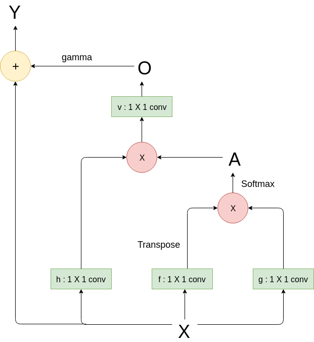
Figure 1: Representation of Self Attention, the symbols mean the same as in Eqn. 2

4.1.2 Channel Attention

It finds the channels wise attention [4] of a feature. It consists of two components squeeze and excitation. Squeeze find the spatial average of each channel and gives an output Z according to

$$\begin{split}Z=GlobalAverage(X)\\ where,Z_{c}=\frac{1}{H\times W}\sum_{i=1}^{H}\sum_{j=1}^{W}X_{i,j}\end{split}$$ (3)

$Z_{c}$ denotes attention for each channel. After finding Z, we use the excitation block to find the attention of each channel i.e A given by

$$\begin{split}A=\sigma(W_{2}\delta(W_{1}Z))\\ Y=A*X\end{split}$$ (4)

where $\sigma$ is sigmoid function and $\delta$ is the ReLU function, W1 and W2 denote the weights of two Fully Connected layers. We have implemented the fully connected layers as 1 X 1 convolution.

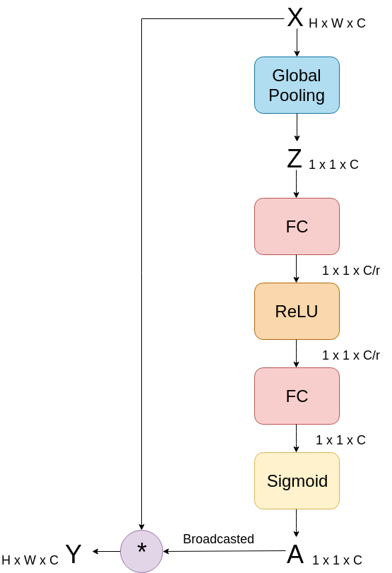
Figure 2: Representation of Channel Attention, the symbols mean the same as in Eqn. 3 Eqn. 4. r is the factor by which the number of channels are initially decreased.

4.1.3 Residual Learning (Skip Connections)

Residual learning can be divided into two types, Global and Local.

In global residual learning we add the input image to the output of the model, it improves the performance of tasks like deblurring were the correlation between the blurred and sharp image is high. This requires the model to only learn the residuals, which are zero in many places, and increases the models learning capability.

Local residual learning was introduced in ResNets. It increasing the learning capability of a model, by reducing over fitting, and allows us to make deeper models.

4.1.4 Spectral Normalization

It is a weight normalization technique [9] used to stabilize the training of GANs. The benefit of spectral normalization is that it only has one hyperparameter to tune i.e Lipschitz Constant and has a low computational cost. In the original paper [9] spectral normalization was only applied to the discriminator, but recent experiments in [18] have shown that applying it to both generator and discriminator gives better results and hence we have done the same.

4.1.5 Edge Information

To check weather edge information gives better performance, we extracted the edges of the sharp images using a Canny Edge Detector [1], and concatenated it with the blurred image as an additional channel, and gave it as input to DeblurGAN model [8].

4.1.6 Feedback Module

LSTM is used between the encoder and decoder of a model to increase its long range dependency. The same image is iterated several times and each time the output of previous iteration’s feedback module is given as input to the current feedback module as shown in Fig. 3

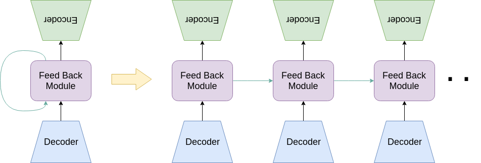
Figure 3: Representation of how a feedback network works.

4.1.7 Classical Losses

The classical losses we used with adversarial loss to help GAN training are L1, L2 and perceptual loss [7]. L1 loss is the average of the absolute difference between the two images, it is determined using the below formula.

$$L_{1}=\frac{\sum\lvert R-S\rvert}{H\times W\times C}$$ (5)

L2 loss is the average of the square of the difference between two images, as shown in the below.

$$L_{2}=\frac{\sum(R-S)^{2}}{H\times W\times C}$$ (6)

It is similar to L2 loss expect that we use the features generated by a particular layer (like conv 3,3 ) of a particular model (like VGG19), instead of images, as shown below.

$$L_{2}=\frac{\sum(\phi(R)-\phi(S))^{2}}{H\times W\times C}$$ (7)

In all the above formulas H, W, C denote the size of the dimensions. R, S denotes the restored (model output) and sharp (target) images. $\phi$ denotes the function (like conv 3, 3 of VGG19) that is used to generate the features.

4.2 Models used

4.2.1 Pix2Pix

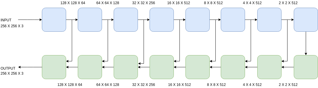
Figure 4: Representation of pix2pix network. Here the blue boxes denote the encoder blocks, while the green boxes denote the decoder blocks

The generator is an encoder decoder structure with skip connections from one encode block to a decode block, similar to U-Net [13] as shown in the figure Fig. 4. Each encode block consists of a convolution with stride 2 and padding “same” to reduce the spatial dimension by half. The number of channels are doubled until they they reach 512, except for the first encode block which

increases the number of channels from 3 to 64. After the convolution we have a batch normalization and ReLU. Similarly each decode block consist of the transpose convolution, batch normalization and ReLU. Where the transpose convolution in contrast to convolution, increases the spatial dimension while decreasing the number of channels. The last decode block has a tanh activation instead of a ReLU. The discriminator used is a Markovian Discriminator (PatchGAN), it takes an N x N patch of a image and predicts weather it is the model output or the target, it does that for each patch and produces an image where each pixel denotes the prediction of the corresponding N x N patch. We average all the responses to get the final output. We used the techniques given above to improve this model for the task of deblurring, the exact details of which are in the Results section.

4.2.2 Residual in Residual Network

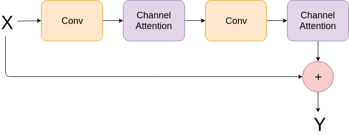
(a) Residual Block

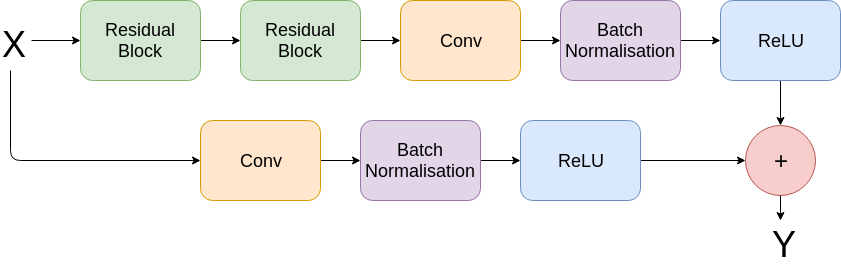
(b) Encoder Module

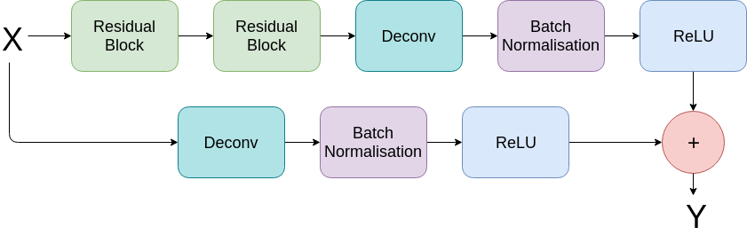
(c) Decoder Module

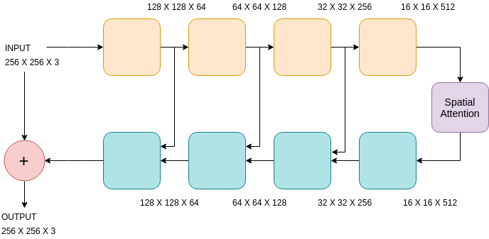
(d) Residual in Residual model with channel and spatial attention, here the orange boxes denote encoder module, while the blue boxes denote the decoder module

As the name suggests, several residual blocks are further given residual connections among them as shown in the Fig. 5(b) 5(c). The networks design is inspired by [20]. The encoder decoder network with several encode and decode blocks is similar to that of pix2pix [6]. But each encode/decode block is a residual in residual block as shown in Fig. 5(d). Each block consists of two Res blocks , a convolution/transpose convolution, a batch norm and a ReLU, the output is added with the input which has been scaled to the proper size after it passes through another convolution. Each of the Res Block consists of two series of convolution and channel

attention, the output of which is added to the input. The model given above and a variant of it was implemented details of which are given in the Result section.

4.2.3 DeblurGAN

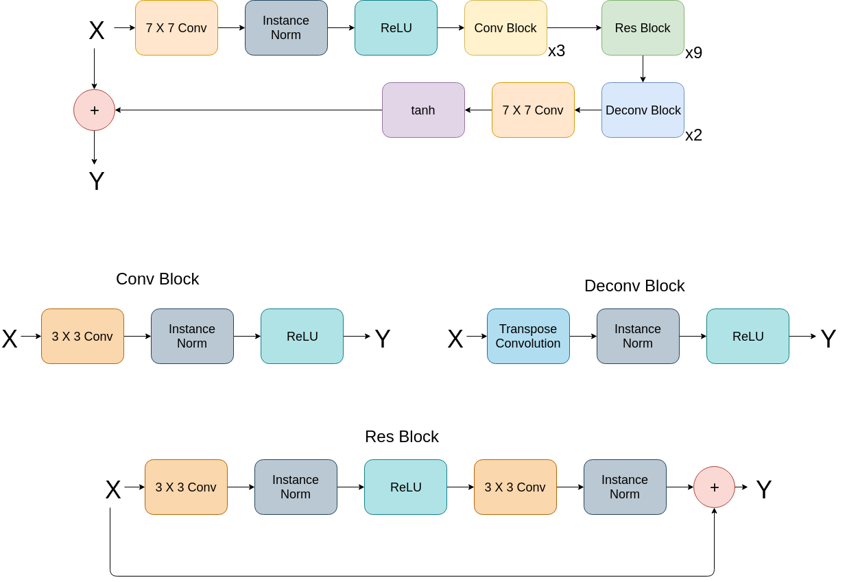
Figure 6: Representation of DeblurGAN [8]

DeblurGAN [8] structure is as shown in Fig. 6. Techniques mentioned above were used to improve its performance, details of which are in the Result section.

4.3 Metrics

4.3.1 PSNR

PSNR can be thought of as the reciprocal of MSE. MSE can be calculated as

$$MSE=\frac{\sum_{H,W}(S-R)^{2}}{H\times W}$$ (8)

where H, W are the size of the dimensions of the image. S and R are the sharp and restored image respectively. Given MSE, PSNR can be calculated using,

$$PSNR=\dfrac{m^{2}}{MSE}$$ (9)

where m is the maximum possible intensity value, since we are using 8-bit integer to represent a pixel in each channel, m = 255.

4.3.2 SSIM

SSIM helps us to find the structural similarity between two image, it can be calculated using,

$$SSIM(x,y)=\dfrac{(2\mu_{x}\mu_{y}+c_{1})(2\sigma_{xy}+c_{2})}{(\mu_{x}^{2}+\mu_{y}^{2}+c_{1})(\sigma_{x}^{2}+\sigma_{y}^{2}+c_{2})}$$ (10)

where x, y are windows of equal dimension for restored and sharp images. $\mu_{x},\mu_{y}$ denotes mean of x, y respectively. $\sigma_{x},\sigma_{y}$ denotes variance for x, y respectively, whereas $\sigma_{xy}$ is the covariance between x and y. $c_{1}$ and $c_{2}$ are constants used to stabilize the division.

4.4 Dataset

GoPro [10] was used for all experiments. To generate this dataset a GoPro Hero5 Black camera was used which captured high resolution (1280 × 720), high frame rate (240 frames per second) videos outdoor. To generate blurred image an average of a few frames (odd number picked randomly from 7 to 23) was taken, while the central frame was considered as the corresponding sharp image. To reduce the magnitude of relative motion across frames they were down sampled and to avoid artifacts caused by averaging only frames were the optical flow was at most 1 were considered.

5 Results

5.1 Pix2pix

Methods	PSNR	SSIM
Pix2Pix	25.41	0.810
Pix2Pix + Sl. Attn	25.41	0.808
Pix2Pix + Sl. Attn + GR	27.29	0.858
Pix2Pix + Sl. Attn + SN	26.05	0.831
Pix2Pix + Sl. Attn + Ch. Attn + GR + SN + Percep. Loss	27.05	0.831

Table 1: PSNR and SSIM for different improvements on the pix2pix model. Sl. Attn refers to Self Attention. GR refers to Global Residual. SN refers to spectral normalization. Ch. Attn refers to Channel. Percep. Loss refers to perceptual loss

In case of addition of attention (only spatial or both spatial and channel), they were added after every three encoder/decoder blocks, with a channel attention between the encoder and the decoder when the feature size 1 x 1 x 512. All test were done on 256 X 256 images. Each model was trained for 50 epochs.

5.2 Residual in Residual

Methods	PSNR	SSIM
RiR + Ch. Attn + Sl. Attn + Percep. Loss + SN + GR	22.70	0.640
RiR(Large) + Ch. Attn + Sl. Attn + L1 Loss + SN + GR	23.46	0.671

Table 2: PSNR and SSIM for different improvements on the Residual in Residual (RiR) model. Sl. Attn refers to Self Attention. GR refers to Global Residual. SN refers to spectral normalization. Ch. Attn refers to Channel. Precep. Loss refers to perceptual loss

The “large” variant is similar to Fig. 5(d), except that it uses one extra encoder as well as decoder block. All models are trained for 300 epochs. RiR model is tested on 1280 X 720 images, while RiR(Large) is tested on 1280 X 768 images.

5.3 DeblurGAN

Methods	PSNR	SSIM
DeblurGAN	28.70	0.958
DeblurGAN + Edge Information	25.27	0.773
DeblurGAN + Feedback	27.20	0.827

Table 3: PSNR and SSIM for different improvements on the DeblurGAN model

Each image is iterated 4 times over the feedback module. Tests are done on 1280 X 720 images. Each model is trained for 300 epochs.

6 Conclusion

Different GAN models were used for the task of deblurring and there performance was improved using various techniques mentioned above. Residual connections (specially global residual) and attention modules, have shown an improvement in performance to the existing model. Use of classical losses and spectral normalization were also helpful for stable GAN training. Use of larger models gave better performance (like in case of RiR and RiR(Large)). Use of edge information and feedback modules seems not to improve the performance of the model. The implementation of the models can be found in the given link https://github.com/lenka98/Bind-Deblurring-using-GANs

Appendices

Appendix A Abbreviations

Below are the abbreviations used:

GAN	Generative Adversarial Network
CNN	Convolutional Neural Network
PSNR	Peak Signal to Noise Ratio
SSIM	Structural Similarity
ReLU	Rectified Linear Unit
FC	Fully Connected
LSTM	Long Short Term Memory
MSE	Mean Square Error

Appendix B Notations

Below are the Notations used.

B	Blurred Image
S	Sharp Image (Ground Truth)
R	Restored Image (Model Output)
K	Blur Kernel
N	Additive Noise
FC	Fully Connected
X	Input to a module
Y	Output of a module
A	Attention Map
O	Intermediate output
$\gamma$	Learnable constant
Z	Squeezed Features
$\sigma$	Sigmoid Activation
$\delta$	ReLU Activation
$W_{i}$	Weight Matrix
H, W, C	Height, Width, and Channels of a feature/image
$\phi$	Function representing a CNN layer
$\mu_{x}$	Mean of x
$\sigma_{x}$	Variance of x
$\sigma_{xy}$	Co-Variance of x w.r.t y

References

- [1] J Canny. A computational approach to edge-detection. Ieee transactions on pattern analysis and machine intelligence, 8(6):679–698, Nov 1986.
- [2] Dong Gong, Jie Yang, Lingqiao Liu, Yanning Zhang, Ian Reid, Chunhua Shen, Anton van den Hengel, and Qinfeng Shi. From motion blur to motion flow: A deep learning solution for removing heterogeneous motion blur. In The IEEE Conference on Computer Vision and Pattern Recognition (CVPR), July 2017.
- [3] Ian Goodfellow, Jean Pouget-Abadie, Mehdi Mirza, Bing Xu, David Warde-Farley, Sherjil Ozair, Aaron Courville, and Yoshua Bengio. Generative adversarial nets. In Z. Ghahramani, M. Welling, C. Cortes, N. D. Lawrence, and K. Q. Weinberger, editors, Advances in Neural Information Processing Systems 27, pages 2672–2680. Curran Associates, Inc., 2014.
- [4] Jie Hu, Li Qin Shen, and Gang Sun. Squeeze-and-excitation networks. 2018 IEEE/CVF Conference on Computer Vision and Pattern Recognition, pages 7132–7141, 2018.
- [5] Gao Huang, Zhuang Liu, Laurens van der Maaten, and Kilian Q. Weinberger. Densely connected convolutional networks. In The IEEE Conference on Computer Vision and Pattern Recognition (CVPR), July 2017.
- [6] Phillip Isola, Jun-Yan Zhu, Tinghui Zhou, and Alexei A. Efros. Image-to-image translation with conditional adversarial networks. In The IEEE Conference on Computer Vision and Pattern Recognition (CVPR), July 2017.
- [7] Justin Johnson, Alexandre Alahi, and Li Fei-Fei. Perceptual losses for real-time style transfer and super-resolution. In European Conference on Computer Vision, 2016.
- [8] Orest Kupyn, Volodymyr Budzan, Mykola Mykhailych, Dmytro Mishkin, and Jiří Matas. Deblurgan: Blind motion deblurring using conditional adversarial networks. In The IEEE Conference on Computer Vision and Pattern Recognition (CVPR), June 2018.
- [9] Takeru Miyato, Toshiki Kataoka, Masanori Koyama, and Yuichi Yoshida. Spectral normalization for generative adversarial networks. In International Conference on Learning Representations, 2018.
- [10] Seungjun Nah, Tae Hyun Kim, and Kyoung Mu Lee. Deep multi-scale convolutional neural network for dynamic scene deblurring. In The IEEE Conference on Computer Vision and Pattern Recognition (CVPR), July 2017.
- [11] Mehdi Noroozi, Paramanand Chandramouli, and Paolo Favaro. Motion deblurring in the wild. CoRR, abs/1701.01486, 2017.
- [12] Sainandan Ramakrishnan, Shubham Pachori, Aalok Gangopadhyay, and Shanmuganathan Raman. Deep generative filter for motion deblurring. CoRR, abs/1709.03481, 2017.
- [13] O. Ronneberger, P.Fischer, and T. Brox. U-net: Convolutional networks for biomedical image segmentation. In Medical Image Computing and Computer-Assisted Intervention (MICCAI), volume 9351 of LNCS, pages 234–241. Springer, 2015. (available on arXiv:1505.04597 [cs.CV]).
- [14] Jian Sun, Wenfei Cao, Zongben Xu, and Jean Ponce. Learning a convolutional neural network for non-uniform motion blur removal. In The IEEE Conference on Computer Vision and Pattern Recognition (CVPR), June 2015.
- [15] Xin Tao, Hongyun Gao, Xiaoyong Shen, Jue Wang, and Jiaya Jia. Scale-recurrent network for deep image deblurring. In The IEEE Conference on Computer Vision and Pattern Recognition (CVPR), June 2018.
- [16] Ashish Vaswani, Noam Shazeer, Niki Parmar, Jakob Uszkoreit, Llion Jones, Aidan N Gomez, Ł ukasz Kaiser, and Illia Polosukhin. Attention is all you need. In I. Guyon, U. V. Luxburg, S. Bengio, H. Wallach, R. Fergus, S. Vishwanathan, and R. Garnett, editors, Advances in Neural Information Processing Systems 30, pages 5998–6008. Curran Associates, Inc., 2017.
- [17] Xiaolong Wang, Ross B. Girshick, Abhinav Gupta, and Kaiming He. Non-local neural networks. CoRR, abs/1711.07971, 2017.
- [18] Han Zhang, Ian Goodfellow, Dimitris Metaxas, and Augustus Odena. Self-attention generative adversarial networks. In Kamalika Chaudhuri and Ruslan Salakhutdinov, editors, Proceedings of the 36th International Conference on Machine Learning, volume 97 of Proceedings of Machine Learning Research, pages 7354–7363, Long Beach, California, USA, 09–15 Jun 2019. PMLR.
- [19] Jiawei Zhang, Jinshan Pan, Jimmy Ren, Yibing Song, Linchao Bao, Rynson W.H. Lau, and Ming-Hsuan Yang. Dynamic scene deblurring using spatially variant recurrent neural networks. In The IEEE Conference on Computer Vision and Pattern Recognition (CVPR), June 2018.
- [20] Yulun Zhang, Kunpeng Li, Kai Li, Lichen Wang, Bineng Zhong, and Yun Fu. Image super-resolution using very deep residual channel attention networks. In The European Conference on Computer Vision (ECCV), September 2018.