Thermal instability through the outer half of quasi-static spherically symmetric molecular clumps and cores

Abstract

Thermal instability (TI) is a trigger mechanism, which can explain formation of condensations through some regions of the interstellar clouds. Our goal here is to investigate some conditions for occurrence of TI and formation of pre-condensations through the outer half a quasi-static spherical molecular clump or core. The inner half is nearly singular and ambiguous so out of scope of this research. We consider a spherically symmetric molecular cloud in quasi-static and thermally equilibrium state, and we use the linear perturbation method to investigate occurrence of TI through its outer half. The origin of perturbations are assumed to be as Inside-Rush-Perturbation (IRP) with outward perturbed velocity at inner region of the cloud, and Outside-Rush-Perturbation (ORP) with inward perturbed velocity originated at the outer parts of the cloud. The local thermal balance at the outer half of the molecular cloud leads to a local loosely constrained power-law relation between the pressure and density as $p\propto\rho^{1+\chi}$, where $-0.4\lesssim\chi\lesssim 0.05$ depends on the functional form of the net cooling function. Physically, the value of $\chi$ depends on the power of dependence of magnetic field to the density, $\eta$, and also on the value of magnetic field gradient, $\zeta$. For strong magnetic field (smaller $\eta$) and/or large field gradient (greater $\zeta$), the value of $\chi$ decreases, and vice versa. The results show that increasing of the value of $\chi$ leads to form a flatter density profiles at the thermally equilibrium outer half of the molecular clump or core, and to occur more thermally unstable IRP and ORP with smaller growth time-scales, and vice versa.

1 Introduction

Molecular clouds have hierarchical structure with dense regions nominated as clumps and cores. These dense regions are nurseries where the stars and planets will birth. Knowing that how these dense regions evolve to form stars and planets is therefore of crucial importance to achieve an appropriate star formation theory. Nowadays, with the help of infrared detectors in large arrays and on the space telescopes, a lot of observational data are available about the specifications of clumps and cores (e.g., Liu et al. 2019, Brunetti & Wilson 2019, Caselli et al. 2019, Sokol et al. 2019). We can deduce from hierarchical structure of molecular clouds that the clumps and cores must also have smaller condensations through their substructures. There is some observational instances for existence of small condensations through clumps and prestellar cores (e.g., Friesen et al. 2014, Kirk et al. 2017, Tokuda et al. 2018, Ohashi et al. 2018)

There are some theoretical aspects explaining the formation of these condensations through the molecular clumps and prestellar cores. For example, the arm-like over-densities through clump G33.92+0.11 may be a natural consequence of the Toomre instability, which can fragment to form young stellar objects in shorter time-scales than the time-scale of the global clump contraction (Liu et al. 2019). The turbulent motions have also been proposed as being important for dynamical evolution of star clusters during their formations from turbulent clumps (e.g., Farias et al. 2019). Another mechanism for the formation of over-dense regions is the effects of magnetic fields on regulating the substructures of molecular clumps (e.g., Bahmani & Nejad-Asghar 2018, Lee & Hennebelle 2019). Since the substructures through the molecular cores have very small masses, and are characterized by subsonic levels of internal turbulence and infall motions (e.g., Lee, Myers & Tafalla 2001), the instability processes produced via the effects of magnetic fields may be more important than gravitational and turbulent effects (e.g., van Loo, Falle, & Hartquist 2007, Nejad-Asghar 2011). Thus, there may be important to consider some non-turbulent and/or non-gravitational instability processes such as thermal instability (TI) for formation of small over-densities through the quiescent regions of the molecular clumps and cores.

After the pioneer paper of Field (1965), entitled thermal instability, this subject appeared to be considered as a mechanism to explain formation of some over-densities through the interstellar clouds (e.g., Hunter 1966, de Gouveia dal piano & Opher 1990, Fukue & Kamaya 2007). Nejad-Asghar (2011) showed that by considering the heating due to ambipolar diffusion in the molecular clouds, the TI criterion can be satisfied in a worthy fashion, so that the mechanism of TI can be used to explain the formation of small condensations in the cylindrical geometry of molecular clouds. Since the self-gravity stratifies the gas, there must be difference between the linear regimes of TI criterions in the different geometries. For example, McCourt et al. (2012) simulated the occurrence of TI and formation of condensations through gravitationally stratified plasmas using simplified plane-parallel geometry, while Choudhury & Sharma (2016) showed that in the non-linear simulations, there are only minor differences in cold gas condensation for different geometries.

Since spherical geometry is more appropriate for the structure of clumps and cores, we use the symmetric spherical geometry approximation to investigate occurrence of TI in the linear regime. In this geometry, the gravitational field is required to keep the gas motionless in spite of its internal pressure, and this field stratifies the gas into layers of varying density. If thermal disturbances are much shorter than a scale height, one would expect the TI to be governed by the considerations of plane-wave approximation. Perturbations with larger scales, however, will necessarily encompass regions of differing densities (and temperatures). The goal of this paper is to investigate whether the large scale perturbations through the quasi-static spherically symmetric thermal equilibrium cloud can lead to TI process and formation of dense regions. For this purpose, the equilibrium profiles of the quasi-static spherically symmetric thermal equilibrium cloud are given in §2. In section 3, the perturbations are applied on the basic equations with considering of net cooling rate as a parametric power-law function. The eigenfunctions, which obtained from perturbing cloud, are solved in §4, and the results are depicted. Finally, section 5 is devoted to a summary and conclusions.

2 Thermal equilibrium state

In spherical polar coordinates, the usual hydrodynamic equations for spherically symmetric molecular cloud are

$$\frac{\partial\rho}{\partial t}+\frac{1}{r^{2}}\frac{\partial}{\partial r}\left(r^{2}\rho u\right)=0,$$ (1)

$$\frac{\partial u}{\partial t}+u\frac{\partial u}{\partial r}+\frac{1}{\rho}\frac{\partial p}{\partial r}+\frac{GM}{r^{2}}=0,$$ (2)

$$\frac{\partial M}{\partial t}+u\frac{\partial M}{\partial r}=0,$$ (3)

$$\frac{\partial p}{\partial t}+u\frac{\partial p}{\partial r}+\gamma p\frac{1}{r^{2}}\frac{\partial}{\partial r}\left(r^{2}u\right)=-\left(\gamma-1\right)\rho\Omega,$$ (4)

$$p=\frac{k_{B}}{\mu m_{H}}\rho T,$$ (5)

where mass density $\rho$, the enclosed mass $M=\int_{0}^{r}4\pi r^{2}\rho dr$, radial flow velocity $u$, thermal gas pressure $p$ and temperature $T$ depend on the radius $r$ and time $t$; the net cooling function is represented by $\Omega(\rho,T)$ that is generally a complicated function of local density and temperature, $G$ is the gravitational constant, $\gamma\approx 5/3$ is the ratio of specific heats, and $k_{B}$, $\mu\approx 2.3$ and $m_{H}$ are Boltzmann constant, the mean molecular weight and the hydrogen mass, respectively.

In the thermally equilibrium state, the net cooling function $\Omega(\rho,T)$ must be zero at each radius $r$ (i.e., locally thermal balance). To calculate the thermal balance within the molecular clumps or cores, we need to consider heating and cooling processes affecting the gas and the dust. Here, we use a general parameterized form of the net cooling function as

$$\Omega(\rho,T)=\Lambda_{0}\rho^{\xi_{1}}T^{\delta_{1}}-\Gamma_{0}\rho^{\xi_{2}}T^{\delta_{2}},$$ (6)

where the estimated values of the coefficients $\Lambda_{0}$ and $\Gamma_{0}$, and the parameters $\xi_{1}$, $\delta_{1}$, $\xi_{2}$ and $\delta_{2}$ are described in the Appendix.

We use the non-dimensional quantities $\tilde{\rho}\equiv\rho/\rho_{i}$, $\tilde{p}\equiv p/p_{i}$, $\tilde{T}\equiv T/T_{i}$, $\tilde{r}\equiv r/(\frac{p_{i}}{4\pi G\rho_{i}^{2}})^{\frac{1}{2}}$, $\tilde{M}\equiv M/4\pi(\frac{p_{i}}{4\pi G\rho_{i}^{2}})^{\frac{3}{2}}\rho_{i}$, $\tilde{t}\equiv t/(\frac{1}{4\pi G\rho_{i}})^{\frac{1}{2}}$, $\tilde{u}\equiv u/(\frac{p_{i}}{\rho_{i}})^{\frac{1}{2}}$, and $\tilde{\Omega}\equiv\Omega/(\frac{4\pi Gp_{i}^{2}}{\rho_{i}})^{\frac{1}{2}}$, where $\rho_{i}$, $T_{i}$, and $p_{i}=\frac{k_{B}\rho_{i}T_{i}}{\mu m_{H}}$ are density, temperature, and pressure, respectively, at the outer boundary of the molecular clump or core (i.e., intercloud medium). In this way, the equations (1)-(6) become

$$\frac{\partial\tilde{\rho}}{\partial\tilde{t}}=-\frac{1}{\tilde{r}^{2}}\frac{\partial}{\partial\tilde{r}}\left(\tilde{r}^{2}\tilde{\rho}\tilde{u}\right),$$ (7)

$$\frac{\partial\tilde{u}}{\partial\tilde{t}}=-\tilde{u}\frac{\partial\tilde{u}}{\partial\tilde{r}}-\frac{1}{\tilde{\rho}}\frac{\partial\tilde{p}}{\partial\tilde{r}}-\frac{\tilde{M}}{\tilde{r}^{2}},$$ (8)

$$\frac{\partial\tilde{M}}{\partial\tilde{t}}=-\tilde{u}\frac{\partial\tilde{M}}{\partial\tilde{r}},$$ (9)

$$\frac{\partial\tilde{p}}{\partial\tilde{t}}=-\tilde{u}\frac{\partial\tilde{p}}{\partial\tilde{r}}-\gamma\tilde{p}\frac{1}{\tilde{r}^{2}}\frac{\partial}{\partial\tilde{r}}\left(\tilde{r}^{2}\tilde{u}\right)-\left(\gamma-1\right)\tilde{\rho}\tilde{\Omega},$$ (10)

$$\tilde{p}=\tilde{\rho}\tilde{T},$$ (11)

$$\tilde{\Omega}(\tilde{\rho},\tilde{T})=\tilde{\Lambda}_{0}\tilde{\rho}^{\xi_{1}}\tilde{T}^{\delta_{1}}-\tilde{\Gamma}_{0}\tilde{\rho}^{\xi_{2}}\tilde{T}^{\delta_{2}},$$ (12)

where $\tilde{\Lambda}_{0}\equiv\Lambda_{0}\rho_{i}^{\xi_{1}}T_{i}^{\delta_{1}}/(\frac{4\pi Gp_{i}^{2}}{\rho_{i}})^{\frac{1}{2}}$ and $\tilde{\Gamma}_{0}\equiv\Gamma_{0}\rho_{i}^{\xi_{2}}T_{i}^{\delta_{2}}/(\frac{4\pi Gp_{i}^{2}}{\rho_{i}})^{\frac{1}{2}}$.

The turbulent energy sources in the molecular clouds can not be continuously maintained (Mac Low & Klessn 2004), i.e., the turbulent energy will decay (Gao, Xu & Law 2015). Assuming the Kolmogorov scaling for eddy turbulent fluctuating velocity (Kolmogorov 1941)

$$v_{eddy}\sim v_{0}\left(\frac{l}{l_{0}}\right)^{1/3},$$ (13)

where $v_{0}\sim 30\,\mathrm{km\,s^{-1}}$ and $l_{0}\sim 100\,\mathrm{pc}$ are suitable for giant molecular clouds (Gao, Xu & Law 2015), the turbulent decay time-scales, $l/v_{eddy}$, in the molecular clumps (with $l\sim\,0.3\mathrm{pc}$) and cores (with $l\sim\,0.03\mathrm{pc}$) are $7\times 10^{4}\mathrm{yr}$ and $1.5\times 10^{4}\mathrm{yr}$, respectively. Since these time-scales are comparable to the cooling time-scales (figure 2 of Nejad-Asghar 2011), we assume that our interesting molecular clumps and cores are approximately in the quasi static state.

The local thermal balance (i.e., $\tilde{\Omega}=0$ at each radius $\tilde{r}$) at the outer half of the clump or core leads to a local relation between pressure and density as $\tilde{p}=\kappa\tilde{\rho}^{(1+\chi)}$, where $\kappa\equiv(\frac{\tilde{\Gamma}_{0}}{\tilde{\Lambda}_{0}})^{\frac{1}{\delta_{1}-\delta_{2}}}$ and $\chi\equiv\frac{\xi_{2}-\xi_{1}}{\delta_{1}-\delta_{2}}$. Using this local relation between pressure and density, the stationary ($\partial/\partial t=0$) quasi-static ($u\rightarrow 0$) state of the equations (1)-(5) become

$$\frac{d\tilde{\rho}}{d\tilde{r}}=-\frac{\tilde{M}\tilde{\rho}^{(1-\chi)}}{\kappa(1+\chi)\tilde{r}^{2}},$$ (14)

$$\frac{d\tilde{M}}{d\tilde{r}}=\tilde{r}^{2}\tilde{\rho},$$ (15)

which can be integrated numerically (e.g., with Runge-Kutta method), from the outer boundary of the spherical cloud $\tilde{r}=1$ with the boundary conditions $\tilde{\rho}_{(\tilde{r}=1)}=1$ and $\tilde{M}_{(\tilde{r}=1)}=\tilde{M}_{c}$, where $\tilde{M}_{c}$ is the total cloud mass in the non-dimensional scale.

According to the estimated values of the parameters $\xi_{1}$, $\xi_{2}$, $\delta_{1}$, and $\delta_{2}$ in the Appendix, we have $\frac{-1.9-0.3}{2.1-0.2}\approx-1.2\lesssim\chi\lesssim\frac{0.2-0.1}{2.1-0.2}\approx 0.05$. Since the pressure gradient through the outer part of the clumps or cores must be a negative value, we have the constraint $(1+\chi)\frac{d\tilde{\rho}}{d\tilde{r}}<0$. On the other hand, we physically expect that the density profile of a self gravitating cloud is a decreasing function versus the radius (i.e., $\frac{d\tilde{\rho}}{d\tilde{r}}$ must be less than $0$), thus, we must have $\chi>-1$. Equations (14) and (15) show that if the value of $\chi$ is near to $-1$, a large value of the density gradient occurs so that the enclosed mass will be reduced to zero very rapidly. This case cannot be physically occurred in the cloud, thus, we choose the minimum allowed value of $\chi$ equal to $-0.5$ so that a suitable small fraction of the total cloud mass will be enclosed in the outer half between the inner radius $\tilde{r}_{in}\approx 0.5$ and the outer region $\tilde{r}=1$. Increasing of the other parameter, $\kappa$, can only decreases the density profile, and vice versa. Here, without loss of generality, we choose $\kappa=1$. The results for density profile and the enclosed mass in the outer half of cloud, with four values of the parameter $\chi$ equal to $-0.4$, $-0.3$, $-0.2$, and $0.05$ are depicted in the Fig. 1.

3 Perturbation analysis

Our goal here is to investigate occurrence of thermal instability through the outer half of a quasi-static spherically symmetric molecular clump or core. We split each variable into unperturbed and perturbed components; the latter is indicated by subscript ’1’, while the equilibrium variables was denoted by subscript ’0’. We apply the linear perturbation analysis with time Fourier expansion, $A_{1}(\tilde{r},\tilde{t})=A_{1}(\tilde{r})\exp(\omega\tilde{t})$, on the outer half of a thermally equilibrium spherical molecular clump or core. Time evolution in the non-linear regime is out of scope of this paper. It is of great interest to derive the growth rate of instability that is the real part of $\omega$. In this way, the equations (7)-(11) can be linearized by repeated use of the unperturbed background equations, (14) and (15), as follows

$$\omega\rho_{1}=-\left(\tilde{\rho}_{0}^{\prime}+\frac{2}{\tilde{r}}\tilde{\rho}_{0}\right)u_{1}-\tilde{\rho}_{0}u_{1}^{\prime},$$ (16)

$$\omega u_{1}=-\frac{\tilde{M}_{0}}{\tilde{r}^{2}\tilde{\rho}_{0}}\rho_{1}-\frac{1}{\tilde{r}^{2}}M_{1}-\frac{1}{\tilde{\rho}_{0}}p_{1}^{\prime},$$ (17)

$$\omega M_{1}=-\tilde{M}_{0}^{\prime}u_{1},$$ (18)

$$\omega p_{1}=-\tilde{T}_{0}(\nu_{\rho}-\nu_{T})\rho_{1}+\left(\frac{\tilde{\rho}_{0}\tilde{M}_{0}}{\tilde{r}^{2}}-\frac{2\gamma\tilde{p}_{0}}{\tilde{r}}\right)u_{1}-\gamma\tilde{p}_{0}u_{1}^{\prime}-\nu_{T}p_{1},$$ (19)

where primes denote $\frac{d}{d\tilde{r}}$, and

$$\nu_{T}\equiv(\gamma-1)\left(\frac{\partial\tilde{\Omega}}{\partial\tilde{T}}\right)_{\tilde{\rho}}=(\gamma-1)\tilde{\Lambda}_{0}\tilde{\rho}_{0}^{\xi_{1}}\tilde{T}_{0}^{\delta_{1}-1}(\delta_{1}-\delta_{2}),$$ (20)

$$\nu_{\rho}\equiv(\gamma-1)\frac{\tilde{\rho}_{0}}{\tilde{T}_{0}}\left(\frac{\partial\tilde{\Omega}}{\partial\tilde{\rho}}\right)_{\tilde{T}}=(\gamma-1)\tilde{\Lambda}_{0}\tilde{\rho}_{0}^{\xi_{1}}\tilde{T}_{0}^{\delta_{1}-1}(\xi_{1}-\xi_{2}),$$ (21)

are angular frequencies of sound waves with isochoric and isothermal perturbations, respectively.

For small disturbances at the outer regions of the spherical cloud (i.e., $k\tilde{r}\rightarrow\infty$, where $k$ is the wavenumber), the plane-wave Fourier expansion, $A_{1}(\tilde{r})=A_{1}^{d}\exp(ik\tilde{r})$, with approximately homogenous medium is suitable, as was investigated in the well-known pioneered work of Field (1965). The Field’s criterions for occurrence of linear thermal instability with plane-wave approximation in the homogeneous medium are

$$\cases{a)\quad\nu_{T}\leqslant 0&for all $\nu_{\rho}$,\cr b)\quad\nu_{\rho}>\nu_{T}&for $\nu_{T}\geqslant 0$,\cr c)\quad\nu_{\rho}<-(\gamma-1)\nu_{T}&for $\nu_{T}\geqslant 0$.}$$ (22)

In our interesting region of molecular clump or core, the first criterion cannot be occurred because we always have $\delta_{1}-\delta_{2}>0$. The second and third criterions can be represented as $\chi<-1$ and $\chi>(\gamma-1)$, respectively. According to the mentioned values of the parameters in the Appendix, we see that only the second criterion, $\chi<-1$, for occurrence of linear thermal instability with plane-wave approximation in the homogeneous medium can be reasonable (Nejad-Asghar & Ghanbari 2003). These classic criterions are for local linear TI in the uniform medium. For non-uniform medium with varying density, the classical criterions (22) are not correct and must be modified (Field 1965). In these cases, it may be possible for occurrence of TI with $\chi>-1$ and/or $\chi<(\gamma-1)$, as will be investigated further for the outer half of the spherical clumps/cors.

For large extended (non-local) disturbances, which the sphericalness cannot be neglected and the gravitational field stratifies the gas into shells of varying density, we must use the general eigenfunction method to find the thermal instability criterions. The generic problem is to reduce the linearized equations (16)-(19) to a set of coupled first-order differential equations. In this way, we have

$$\frac{du_{1}}{d\tilde{r}}=-\left(\frac{\tilde{\rho}_{0}^{\prime}}{\tilde{\rho}_{0}}+\frac{2}{\tilde{r}}\right)u_{1}-\frac{\omega}{\tilde{\rho}_{0}}\rho_{1},$$ (23)

$$\frac{dp_{1}}{d\tilde{r}}=\tilde{\rho}_{0}\left(\frac{\tilde{M}_{0}^{\prime}}{\omega\tilde{r}^{2}}-\omega\right)u_{1}-\frac{\tilde{M}_{0}}{\tilde{r}^{2}}\rho_{1},$$ (24)

$$\frac{d\omega}{d\tilde{r}}=0,$$ (25)

where

$$\rho_{1}=\frac{1}{\tilde{T}_{0}(\nu_{\rho}-\nu_{T}-\gamma\omega)}\left\{\left[\frac{\tilde{\rho}_{0}\tilde{M}_{0}}{\tilde{r}^{2}}-\frac{2\gamma\tilde{p}_{0}}{\tilde{r}}+\gamma\tilde{T}_{0}\tilde{\rho}_{0}\left(\frac{\tilde{\rho}_{0}^{\prime}}{\tilde{\rho}_{0}}+\frac{2}{\tilde{r}}\right)\right]u_{1}-(\omega+\nu_{T})p_{1}\right\}.$$ (26)

Imposing three boundary conditions for this set of three coupled first-order differential equations turns it into an eigenvalue problem for $\omega$. The eigenfunctions $u_{1}$ and $p_{1}$, and consequently $\rho_{1}$ and $M_{1}$, can also be obtained with initial guess for $\omega$ and finding its best value to satisfy the boundary conditions.

The physical conditions of the problem present the constraints in the boundaries $\tilde{r}_{in}$ and $\tilde{r}_{out}$. Here, we consider two cases for occurrence of perturbations in the outer half of clumps and/or cores. The first is that outflows from the central region lead to occur of perturbed gas in the inner radius boundary $\tilde{r}_{in}$ with velocity $u_{max}$. The second case is that the perturbations are produced from inflow of material (e.g., outflows from neighbor clumps or cores) at the outer radius boundary $\tilde{r}_{out}$ with inflow velocity $-u_{max}$. In both of these models, we assume that the perturbation of pressure at the boundaries are zero. In this way, we consider two perturbation cases as follows:

• Inside-Rush-Perturbations (IRP) with three two-point boundary conditions

  $$u_{1(\tilde{r}_{in}=0.5)}=+u_{max},\quad p_{1(\tilde{r}_{in}=0.5)}=0,\quad p_{1(\tilde{r}_{out}=1)}=0.$$ (27)

• Outside-Rush-Perturbations (ORP) with three two-point boundary conditions

  $$u_{1(\tilde{r}_{out}=1)}=-u_{max},\quad p_{1(\tilde{r}_{out}=1)}=0,\quad p_{1(\tilde{r}_{in}=0.5)}=0.$$ (28)

4 Results

We must solve the set of three coupled first-order differential equations (23)-(25) with two-point boundary value conditions (27) or (28). There are six parameters in the net cooling function (12) that can specify the occurrence of thermal instability through the outer half of a molecular clump or core: $0.1\lesssim\xi_{1}\lesssim 0.3$, $2.1\lesssim\delta_{1}\lesssim 2.6$, $-1.9\lesssim\xi_{2}\lesssim 0.2$, $0\lesssim\delta_{2}\lesssim 0.2$, $\tilde{\Lambda}_{0}$ and $\tilde{\Gamma}_{0}$. In the thermally equilibrium state, these six parameters reduced into two parameters $\kappa\equiv(\frac{\tilde{\Gamma}_{0}}{\tilde{\Lambda}_{0}})^{\frac{1}{\delta_{1}-\delta_{2}}}$ and $\chi\equiv\frac{\xi_{2}-\xi_{1}}{\delta_{1}-\delta_{2}}$, and we plot some interesting profiles of them in the Fig. 1. In the perturbed state, we reached to a two-point boundary value problem (23)-(25) with boundary conditions (27) or (28).

Using the shooting method (e.g., Press et al. 1992) to find the solutions of these two-point boundary value differential equations show that the results are not sensitive to the parameters $\xi_{1}$, $\delta_{1}$ and $\delta_{2}$. Thus, we choose their median values $\xi_{1}\approx 0.2$, $\delta_{1}\approx 2.4$ and $\delta_{2}\approx 0.1$ for subsequent runs. Also, $u_{max}$ is chosen equal to $0.01$. The results show that increasing of velocity perturbation amplitude $u_{max}$ cannot change the eigenvalue $\omega$ but can modify the eigenfunctions with amplification of their domains (see, e.g., Fig 2). According to the parameters $\kappa$ and $\chi$, we can obtain different plots of the eigenfunctions and their relevant eigenvalues $\omega$. By choosing $\kappa=1$, some typical eigenfunctions $u_{1}$ and $p_{1}$, with some values of the parameter $\chi$, are shown in the Fig. 3. Finding the solutions revealed that the IRP and ORP cases lead to the same results for the eigenvalue $\omega$. According to the plane-fits of cooling and heating functions in the Appendix, the coefficients $\Gamma_{0}$ and $\Lambda_{0}$ are estimated to be in the same order so that the parameter $\kappa$ will be near $\sim 1$. We show the Fig. 4 for dependence of eigenvalues $\omega$ on the parameters $\chi$ and different values of the parameter $\kappa\sim 1$.

5 Summary and conclusions

Molecular clouds have dense substructures, and similar over-density substructures are also found through smaller dimensions of clumps and cores. The existence of the small dense substructures is very important to achieve a comprehensive theory for stars and planets formation. In this paper, we sought to find an idea about the origin of these small dense substructures within the molecular clumps and cores. An idea that may seem important is the TI process. For this purpose, we considered a molecular cloud with spherical and quasi-static approximation and examined the conditions for thermal instability in its outer half. The profiles of density and enclosed mass of the thermally equilibrium states are shown in the Fig. 1.

To investigate the conditions for occurrence thermal instability, we used the linear perturbation method. The most important factor in thermal instability is the functional form of the net cooling function. Here, we used a general parameterized power-law form for the net cooling function (see, Appendix). We considered the origin of the perturbations as the IRP and the ORP, and we solved the differential equations governing the perturbations. Two important parameters are $\chi$ and $\kappa$. Physically, the value of $\chi$ depends on the power of dependence of magnetic field to the density, $\eta$, and the magnetic field gradient, $\zeta$. For strong magnetic field (smaller $\eta$) and/or large field gradient (greater $\zeta$), the minus value of $\chi$ increases, and vice versa. We obtained the eigenfunctions and eigenvalues with the various values of this parameter, and the results are plotted in the Figures 3 and 4.

It is clear from the Fig. 3 that the boundary condition is satisfied in outer and inner regions (i.e., $p_{1}\rightarrow 0$ at $\tilde{r}\rightarrow 0.5\,\mathrm{and}\,1.0$). The results show that the pressure perturbations $p_{1}$ are reversed in the IRP and ORP cases. Also, absolute value of the pressure perturbations in the inner regions are greater than the outer regions. On the other hand, the absolute value of radial velocity perturbations $u_{1}$ in the IRP cases are approximately decreasing from inner region (place of perturbation start) to outer area of the clump or core, while in the ORP it is an approximately increasing function from the place of perturbation start (i.e., outer region). Increasing of absolute value of the velocity perturbation from outer region to inner region is from gravitational force acceleration. Also, the results show that increasing of $\chi$ decreases the absolute value of velocity and pressure perturbations. We conclude from Fig. 4 that increasing of $\chi$ and/or decreasing of $\kappa$ increases the value of $\omega$ so that the TI growth time-scales decreases. Decreasing of the parameter $\kappa$ means the importance of heating coefficient in relative to the cooling coefficient. Fig. 4 reveals that considering the most valuable heating rates (specially the heating due to ambipolar diffusion) can lead to more thermally unstable conditions in the outer half of clumps/cores.

For better understanding of the values presented in the Figures 1-4, it is best to use the dimensional quantities. By choosing $10\mathrm{K}$ for temperature and $10^{3}\mathrm{cm^{-3}}$ for density, as references for the intercloud medium (i.e., at the outer boundary of the spherical cloud), the dimension of length, time, velocity, mass, and net cooling rate are

$$0.1\left(\frac{T_{i}}{10\mathrm{K}}\right)^{\frac{1}{2}}\left(\frac{n_{i}}{10^{3}\mathrm{cm^{-3}}}\right)^{-\frac{1}{2}}\,\mathrm{pc},$$ (29)

$$5.7\times 10^{5}\left(\frac{n_{i}}{10^{3}\mathrm{cm^{-3}}}\right)^{-\frac{1}{2}}\,\mathrm{yr},$$ (30)

$$1.9\times 10^{4}\left(\frac{T_{i}}{10\mathrm{K}}\right)^{\frac{1}{2}}\,\frac{\mathrm{cm}}{\mathrm{s}},$$ (31)

$$1.0\left(\frac{T_{i}}{10\mathrm{K}}\right)^{\frac{3}{2}}\left(\frac{n_{i}}{10^{3}\mathrm{cm^{-3}}}\right)^{-\frac{1}{2}}\,\mathrm{M_{\odot}},$$ (32)

$$2.1\times 10^{-5}\left(\frac{T_{i}}{10\mathrm{K}}\right)\left(\frac{n_{i}}{10^{3}\mathrm{cm^{-3}}}\right)^{\frac{1}{2}}\,\mathrm{erg}\,\mathrm{g^{-1}s^{-1}},$$ (33)

respectively.

As we can see, if we choose the temperature and density of the intercloud medium equal to $100\mathrm{K}$ and $10^{3}\mathrm{cm^{-3}}$, respectively, then we face a clump of dimension $0.3\mathrm{pc}$ and mass $30\mathrm{M_{\odot}}$. On the other hand, if we choose the temperature and density of the intercloud medium equal to $10\mathrm{K}$ and $10^{4}\mathrm{cm^{-3}}$, respectively, then we will encounter a size and mass equal to $0.03\mathrm{pc}$ and $0.3\mathrm{M_{\odot}}$, respectively, which represents a typical low-mass molecular cloud core. According to the Fig. 4, the growth time-scale of TI through the outer half of these clumps and cores is approximately in the range of $0.1-0.5\,\mathrm{Myr}$ according to different values of the parameters $\chi$ and $\kappa$. In any case, increasing of the parameter $\chi$ and/or decreasing of the parameter $\kappa$ leads to occurrence of more thermally unstable IRP and ORP with smaller growth time-scales. Therefore, as can be seen, thermal instability can be considered as an effective mechanism in the formation of dense regions in the outer half region of clumps and cores.

Appendix A Cooling and heating rates

Here, we briefly present the important cooling and heating processes in the molecular clumps and cores, and the plane-fits are approximated on the plots to determine the valuable ranges of the parameters in the parameterized equation (6). Some most important cooling and heating mechanisms in the molecular clouds are presented in the section 2 of Nejad-Asghar (2011), for variety of densities and temperatures between $10^{3}<n(\mathrm{H_{2}})<10^{10}\mathrm{cm^{-3}}$ and $10<T<200\mathrm{K}$, respectively. Nejad-Asghar (2011) used the cooling function based on the work of Neufeld et al. (1995) which allowed him to include cooling from potentially important coolants of five molecules and two atomic species: $\mathrm{CO}$, $\mathrm{H_{2}}$, $\mathrm{H_{2}O}$, $\mathrm{O_{2}}$, $\mathrm{HCl}$, $\mathrm{C}$, and $\mathrm{O}$. The results presented in figures $3a-3d$ of Neufeld et al. (1995) are convenient to do rough parametrization like the equation

$$\Lambda_{(n,T)}=\Lambda_{(n)}\left(\frac{T}{10\mathrm{K}}\right)^{\beta_{(n)}},$$ (A1)

which was introduced by Goldsmith (2001), and the parameters are given in the figure 1 of Nejad-Asghar (2011).

For the heating sources in the molecular clouds, we consider heating due to cosmic rays, turbulence heating, gravitational work, and dissipation of magnetic energy. Nejad-Asghar (2011) collected the values of the heating due to cosmic rays and turbulence heating to obtain approximately a constant value qual to $\Gamma_{CR}+\Gamma_{TR}\sim 4.1\times 10^{-4}\mathrm{erg\,g^{-1}\,s^{-1}}$. An estimation for the heating produced by the self-gravitational work can be derived directly from the rate of work per particle, $pd(n^{-1})/dt$, and is given by

$$\Gamma_{GR} \approx \frac{p}{nt_{cn}}$$ (A2)

$$\approx 3.9\times 10^{-5}\left(\frac{T}{10\mathrm{K}}\right)\left(\frac{n}{10^{6}\mathrm{cm^{-3}}}\right)^{1/2}\quad\mathrm{erg\,g^{-1}\,s^{-1}},$$

where we have taken $dn/dt\approx n/10t_{ff}$ where $t_{ff}=\sqrt{\frac{3\pi}{32Gmn}}\approx 3.5\times 10^{4}\left(\frac{10^{6}\mathrm{cm^{-3}}}{n}\right)^{1/2}\mathrm{yr}$ is the free-fall time-scale.

The dissipation of magnetic energy would be considered as another heating mechanism, if this energy is not simply radiated away by atoms, molecules, and grains. The major field dissipation mechanism in the dense clouds is almost certainly ambipolar diffusion, which was examined by Scalo (1977) for density dependency of magnetic field in a fragmenting molecular cloud. In the limit of low ionization fraction (i.e., $\rho=\rho_{n}+\rho_{i}\approx\rho_{n}$, where $\rho_{n}$ and $\rho_{i}$ are neutral and ion densities, respectively), the inertia of charged particles being negligible so that the Lorentz force $\textbf{f}_{L}=\frac{1}{4\pi}(\nabla\times\textbf{B})\times\textbf{B}$ will be balanced by the equally important drag force per unit volume

$$\textbf{f}_{d}=\gamma_{AD}\rho_{i}\rho\textbf{v}_{d}=\gamma_{AD}\epsilon\rho^{3/2}\textbf{v}_{d},$$ (A3)

where $\gamma_{AD}\sim 3.5\times 10^{13}\mathrm{cm^{3}\,g^{-1}\,s^{-1}}$ is the collisional drag coefficient in the molecular clouds, $\textbf{v}_{d}$ is the drift velocity of ions in rest of the neutral particles, and we used the relation $\rho_{i}=\epsilon\rho^{1/2}$ between ion and neutral densities in the local ionization equilibrium state with $\epsilon\sim 3\times 10^{-16}\mathrm{g^{1/2}\,cm^{-3/2}}$ (Shu 1992). In this way, the drift velocity of ions, with velocity $\textbf{v}_{i}$, relative to the neutrals with velocity $\textbf{v}_{n}$, is

$$\textbf{v}_{d}=\textbf{v}_{i}-\textbf{v}_{n}\approx\frac{1}{4\pi\gamma_{AD}\epsilon\rho^{3/2}}(\nabla\times\textbf{B})\times\textbf{B}.$$ (A4)

The magnitude of drift velocity, $v_{d}$, is inversely proportional to the power of density and directly proportional to the magnetic field strength and its gradient. Shu (1992, Equation 27.9) used typical values of $B\Delta B/\Delta x\sim(30\mu\mathrm{G})^{2}/0.1\mathrm{pc}$ to estimate the typical drift speeds through the molecular clouds. Li, Myers & McKee (2012) divided the magnetic field into a steady component and a fluctuating one, and used the mean squared method to estimate upper limits on the drift speed. Here, we use the parametric relation $v_{d}=B\zeta\rho^{-3/2}/4\pi\gamma_{AD}\epsilon$, where the parameter $\zeta\equiv\Delta B/\Delta x$ is the change of magnetic field strength in the length-scale $\Delta x$. In this way, the heating due to ambipolar diffusion can be presented as

$$\Gamma_{AD}=\frac{\textbf{f}_{d}.\textbf{v}_{d}}{\rho}=\frac{B^{2}\zeta^{2}}{16\pi^{2}\gamma_{AD}\epsilon}\rho^{-2.5}.$$ (A5)

The magnetic field strength, $B$, is evaluated in the Troland & Crutcher (2008) for a set of $34$ molecular cloud cores. Their evaluations show that the magnetic field strengths are in the range of $0.5$ to $50\,\mathrm{\mu G}$. The authors use a scaling relation of the field strength with density, which is usually parameterized as a power law, $B\propto\rho^{\eta}$ (Crutcher 2012). In the strong-field models, $\eta\lesssim 0.5$ is predicted (e.g., Mouschovias & Ciolek 1999), while for the weak magnetic fields, we have $\eta\approx 0.66$ (Mestel 1966). Here, we use the power-law approximation as $B\approx 100\,\mathrm{\mu G}\left(\frac{n}{10^{6}\,\mathrm{cm}^{-3}}\right)^{\eta}$, where $0.3\lesssim\eta\lesssim 0.6$. In this way, the heating rate due to ambipolar diffusion can be represented as

$$\Gamma_{AD}=2.6\times 10^{-8}\left(\frac{\zeta}{1\,\mathrm{\mu G}/1\,\mathrm{mpc}}\right)^{2}\left(\frac{n}{10^{6}\mathrm{cm}^{-3}}\right)^{-2.5+2\eta}\,\mathrm{erg\,g^{-1}\,s^{-1}},$$ (A6)

where $\zeta\sim 1\,\mathrm{\mu G}/1\,\mathrm{mpc}$ is suitable for outer half of the molecular clumps and cores with strong magnetic field and field gradient (Nejad-Asghar 2016). For weak magnetized clumps/cores, we have $\zeta<<1\,\mathrm{\mu G}/1\,\mathrm{mpc}$ so that the heating due to ambipolar diffusion is negligible.

Here, we focus our attention to the outer half of the molecular clumps and cores with temperatures less than $200~{}\mathrm{K}$ and densities between $10^{3}$ to $10^{5}\,\mathrm{cm^{-3}}$. The heating time-scale can be approximated as $3k_{B}T/2\mu m_{H}\Gamma$ where $\Gamma$ denotes the heating rates due to the cosmic rays and turbulence (CR+TR), the gravitational work (GR), and the ambipolar diffusion (AD), for evaluation of each time-scales, respectively. To present a quantitative comparison between different heating mechanisms, the heating time-scales are plotted in the Fig. 5. As can be seen, in the dilute regions of the outer half of the clumps and cores with smaller densities, the heating due to ambipolar diffusion dominates, while in the inner regions with larger densities, importance of the ambipolar diffusion heating is faded.

In general, the cooling and heating rates are complicated functions of density and temperature. The plots of cooling and heating rates, for temperatures less than $200~{}\mathrm{K}$ and densities between $10^{3}$ to $10^{5}\,\mathrm{cm^{-3}}$, are given in Fig. 6. We can approximate some plane-fits to these plots as follows

$$\log\Lambda=\log\Lambda_{0}+\xi_{1}\log\rho+\delta_{1}\log T,$$ (A7)

$$\log\Gamma=\log\Gamma_{0}+\xi_{2}\log\rho+\delta_{2}\log T,$$ (A8)

where $\Lambda_{0}$ and $\Gamma_{0}$ are constants in the same orders, and the parameters $\xi_{1}$, $\delta_{1}$ and $\delta_{2}$ can be estimated as $0.1\lesssim\xi_{1}\lesssim 0.3$, $2.1\lesssim\delta_{1}\lesssim 2.6$ and $0\lesssim\delta_{2}\lesssim 0.2$. The most important parameter is $\xi_{2}$ which depends on the approximated value of $\zeta$ and the chosen value of $\eta$. Increasing the value of $\zeta$ and/or decreasing the value of $\eta$ (i.e., stronger magnetic field and field gradient) leads to increase the absolute value of slope of the fitted plane in the $\log n$ direction. For molecular clumps and cores with weak magnetic field and field gradients, the heating rates due to cosmic rays, turbulence and gravitational works dominate so that $\xi_{2}$ will be positive. Here, we choose $-1.9\lesssim\xi_{2}\lesssim 0.2$ to consider approximately all suitable situations (in our interesting models) of the gas in the outer half of the molecular clumps and/or cores.

Figure 1: The profiles of density and enclosed mass (in $\log_{10}$ scale) of the thermally equilibrium states in the outer half of a quasi-static spherically symmetric molecular clump or core. The non-dimensional quantities are $\tilde{\rho}\equiv\rho/\rho_{i}$, $\tilde{r}\equiv\left(\frac{k_{B}T_{i}}{4\pi G\mu m_{H}\rho_{i}}\right)^{\frac{1}{2}}$, and $\tilde{M}\equiv 4\pi\left(\frac{k_{B}T_{i}}{4\pi G\mu m_{H}\rho_{i}}\right)^{\frac{3}{2}}\rho_{i}$, where $\rho_{i}$ and $T_{i}$ are density and temperature of intercloud medium, respectively.

Figure 2: The maximum of the absolute value of pressure perturbations in the outer half of the clump/core with $\kappa=1$ and $\chi=-0.2$ versus different values of the input boundary velocity $u_{max}$.

(a)

(b)

Figure 3: The eigenfunctions of (a) velocity perturbations $u_{1}$ and (b) pressure perturbations $p_{1}$, for IRP and ORP with $\kappa=1$ and $\chi=-0.4$ (solid), $\chi=-0.3$ (dash), $\chi=-0.2$ (dot), and $\chi=0.05$ (dash-dot).

Figure 4: The eigenvalues of IRP and ORP perturbations versus the parameters $\kappa$ and $\chi$.

Figure 5: The heating time-scales of cosmic rays and turbulence (CR+TR), gravitational work (GR), and ambipolar diffusion (AD) with two values of $\eta$ for $T=10\,\mathrm{K}$ (solid) and $T=100\,\mathrm{K}$ (dash).

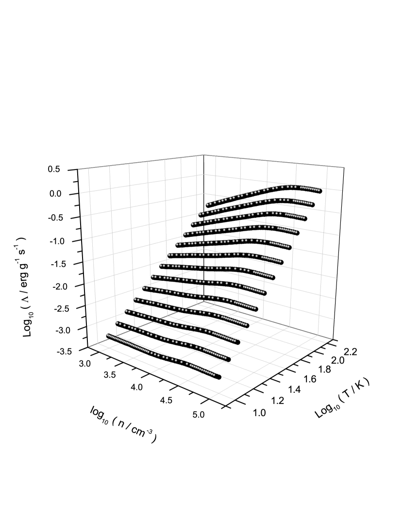
(a)

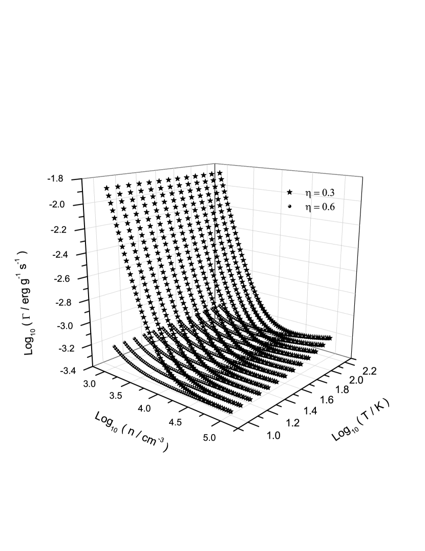
(b)

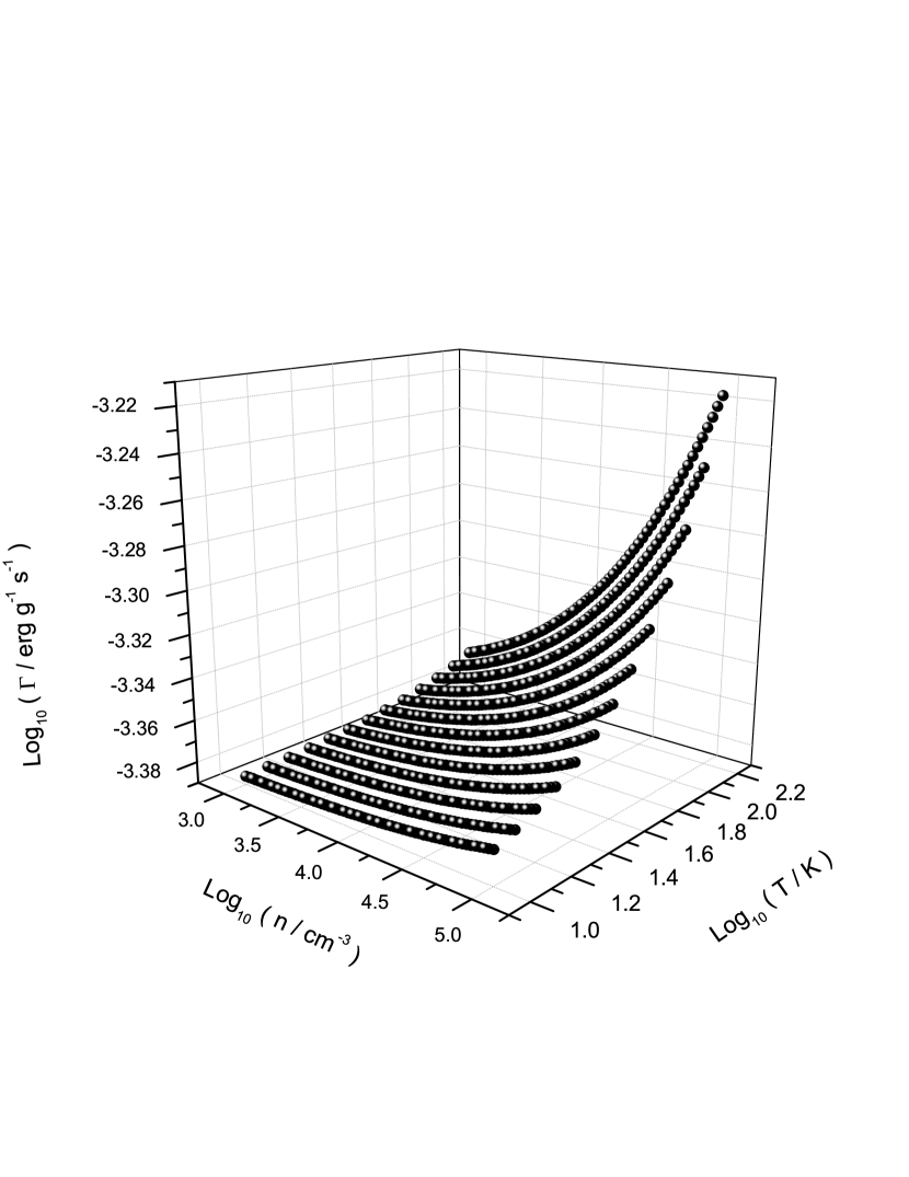
(c)

Figure 6: Three dimensional plots of the (a) cooling rate, (b) heating rates with strong magnetic field ($\zeta\sim 1\,\mathrm{\mu G}/1\,\mathrm{mpc}$) and (c) heating rate with weak magnetic field ($\zeta\rightarrow 0$).

References

- (1) Bahmani, N., Nejad-Asghar, M., 2018, Ap&SS, 363, 171
- (2) Brunetti, N., Wilson, C.D., 2019, MNRAS, 483, 1624
- (3) Caselli, P., Pineda, J.E., Zhao, B., Walmsley, M.C., Keto, E., Tafalla, M., Chacon-Tanarro, A., Bourke, T.L., Friesen, R., Galli, D., Padovani, M., 2019, ApJ, in press (arXiv190205299C)
- (4) Choudhury, P.P., Sharma, P., 2016, MNRAS, 457, 2554
- (5) Crutcher, R.M., 2012, ARA&A, 50, 29
- (6) de Gouveia dal Pino, E.M., Opher, R., 1990, A&A, 231, 571
- (7) Farias, J.P., Tan, J.C., Chatterjee, S., 2019, MNRAS, 483, 4999
- (8) Field, G.B., 1965, ApJ, 142, 531
- (9) Friesen, R.K., Di Francesco, J., Bourke, T.L., Caselli, P., Jørgensen, J.K., Pineda, J.E., Wong, M., 2014, ApJ, 797, 27
- (10) Fukue, T., Kamaya, H., 2007, ApJ, 669, 363
- (11) Gao, Y., Xu, H., Law, C.K., 2015, ApJ, 799, 227
- (12) Glassgold, A.E., Langer, W.D., 1973, ApJ, 179, 147
- (13) Goldsmith, P.F, 2001, ApJ, 557, 736
- (14) Hunter, J.H., 1966, MNRAS, 133, 239
- (15) Kirk, H., Dunham, M.M., Di Francesco, J., Johnstone, D., Offner, S.S.R., Sadavoy, S.I., Tobin, J.J., Arce, H.G., Bourke, T.L., Mairs, S., Myers, P.C., Pineda, J.E., Schnee, S., Shirley, Y.L., 2017, ApJ, 838, 114
- (16) Kolmogorov, A., 1941, DoSSR, 30, 301
- (17) Lee, C.W., Myers, P.C., Tafalla, M., 2001, ApJS, 136, 703
- (18) Lee, Y., Hennebelle, P., 2019, A&A, 622, 125
- (19) Li, P.S., Myers, A., McKee, C.F., 2012, ApJ, 760, 33
- (20) Liu, H. B., Chen, H.V., Román-Zúñiga, C.G., Galván-Madrid, R., Ginsburg, A., Ho, P.T.P., Minh, Y.C., Jiménez-Serra, I., Testi, L., Zhang, Q., 2019, ApJ, 871, 185
- (21) Mac Low, M., Klessen, R.S., 2004, RvMP, 76, 125
- (22) McCourt, M., Sharma, P., Quataert, E., Parrish, I.J., 2012, MNRAS, 419, 3319
- (23) Mestel L., 1966, MNRAS, 133, 265
- (24) Mouschovias T.C., Ciolek G.E., 1999, The Origin of Stars and Planetary Systems, ed. C.J. Lada, N.D. Kylafis, p. 305, Dordrecht: Kluwer
- (25) Nejad-Asghar, M., Ghanbari, J., 2003, MNRAS, 345, 1323
- (26) Nejad-Asghar, M., 2011, MNRAS, 414, 470
- (27) Nejad-Asghar, M., 2016, Ap&SS, 361, 384
- (28) Neufeld, D.A., Lepp, S., Melnick, G.J., 1995, ApJS, 100, 132
- (29) Ohashi, S., Sanhueza, P., Sakai, N., Kandori, R., Choi, M., Hirota, T., Nguyên-Luong, Q., Tatematsu, K., 2018, ApJ, 856, 147
- (30) Press, W.H., Teukolsky, S.A., Vetterling, W.T., Flannery, B.P., 1992, Numerical recipes in FORTRAN. The art of scientific computing, 2nd ed., Cambridge University Press
- (31) Scalo, J.M., 1977, ApJ, 213, 705
- (32) Shu, F.H., 1992, The Physics of Astrophysics: Gas Dynamics, University Science Books, p. 360
- (33) Sokol, A.D., Gutermuth, R.A., Pokhrel, R., Gómez-Ruiz, A.I., Wilson, G.W., Offner, S.S.R., Heyer, M., Luna, A., Schloerb, F.P., Sánchez, D., 2019, MNRAS, 483, 407
- (34) Tokuda, K., Onishi, T., Saigo, K., Matsumoto, T., Inoue, T., Inutsuka, S., Fukui, Y., Machida, M.N., Tomida, K., Hosokawa, T., Kawamura, A., Tachihara, K., 2018, ApJ, 862, 8
- (35) Troland, T.H., Crutcher, R.M., 2008, ApJ, 680, 457
- (36) van Loo, S., Falle, S.A.E.G., Hartquist, T.W., 2007, MNRAS, 376, 779
(a)
(b)
(a)
(b)
(c)