On the long time asymptotic behaviour of the modified Korteweg de Vries equation with step-like initial data

Abstract

We study the long time asymptotic behaviour of the solution $q(x,t)$, $x\in\mathbb{R}$, $t\in\mathbb{R}^{+}$, of the modified Korteweg de Vries equation (MKdV) $q_{t}+6q^{2}q_{x}+q_{xxx}=0$ with step-like initial datum

$$q(x,0)\to\begin{cases}c_{-}\quad\mbox{ for $x\to-\infty$}\\ c_{+}\quad\mbox{ for $x\to+\infty$},\end{cases}$$

with $c_{-}>c_{+}\geq 0$. For the step initial data

$$q(x,0)=\begin{cases}c_{-}\quad\mbox{ for $x\leq 0$},\\ c_{+}\quad\mbox{ for $x>0$},\end{cases}$$

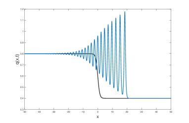
the solution develops an oscillatory region called dispersive shock wave region that connects the two constant regions $c_{+}$ and $c_{-}$. We show that the dispersive shock wave is described by a modulated periodic travelling wave solution of the MKdV equation where the modulation parameters evolve according to a Whitham modulation equation. The oscillatory region is expanding within a cone in the $(x,t)$ plane defined as $-6c_{-}^{2}+12c_{+}^{2}<\frac{x}{t}<4c_{-}^{2}+2c_{+}^{2},$ with $t\gg 1$.

For step-like initial data we show that the solution decomposes for long times in three main regions:

• a region where solitons and breathers travel with positive velocities on a constant background $c_{+}$;

• an expanding oscillatory region (that generically contains breathers);

• a region of breathers travelling with negative velocities on the constant background $c_{-}$.

When the oscillatory region does not contain breathers, the form of the asymptotic solution coincides up to a phase shift with the dispersive shock wave solution obtained for the step initial data. The phase shift depends on the solitons, breathers and the radiation of the initial data. This shows that the dispersive shock wave is a coherent structure that interacts in an elastic way with solitons, breathers and radiation.

1 Introduction

We consider the Cauchy problem for the focusing modified Korteweg–de Vries (MKdV) equation

$$q_{t}(x,t)+6q^{2}(x,t)q_{x}(x,t)+q_{xxx}(x,t)=0,\quad x\in\mathbb{R},\;t\in\mathbb{R}^{+},$$ (1.1)

with a step–like initial datum $q_{0}(x)$ of the form

$$q(x,0)=q_{0}(x)\to c_{\pm}\qquad{\rm as}\quad x\to\pm\infty,$$ (1.2)

where $c_{\pm}$ are some real constants. We are interested in the long-time behavior of the solution.

Due to symmetries $q\mapsto-q$ and $x\mapsto-x,t\to-t,$ it is enough to consider the case

$$c_{-}\geq|c_{+}|,$$ (1.3)

since the other cases of mutual location of the constants $c_{-},c_{+}$ can be reduced to it; however, the cases $c_{-}>c_{+}\geq 0$ and $c_{-}>0>c_{+}\geq-c_{-}$ though qualitatively similar, leads to a quite different asymptotic analysis. In the present manuscript we restrict ourselves to the case $c_{-}>c_{+}\geq 0$ and we discuss briefly the differences with respect to the case $c_{+}<0,$ $|c_{+}|\leq c_{-}$ in the Appendix B.

The focusing MKdV equation is a canonical model for the description of nonlinear long waves when there is a polarity symmetry, and it has many physical applications; in particular, this includes waves in a quantized film [68] internal ocean waves [72], ion acoustic waves in a two component plasma [69]. The MKdV equation is an integrable equation [73] with an infinite number of conserved quantities. For the class of initial data considered, the classical mass and momentum have to be replaced by the conserved quantities

$$\begin{split}&H_{0}=\int\limits_{-\infty}^{x}(q(\widetilde{x},t)-c_{-})\mathrm{d}\widetilde{x}+\int\limits_{x}^{+\infty}(q(\widetilde{x},t)-c_{+})\mathrm{d}\widetilde{x}+(c_{-}-c_{+})x-2(c_{-}^{3}-c_{+}^{3})t,\\ &H_{1}=\int\limits_{-\infty}^{x}(q^{2}(\widetilde{x},t)-c^{2}_{-})\mathrm{d}\widetilde{x}+\int\limits_{x}^{+\infty}(q^{2}(\widetilde{x},t)-c^{2}_{+})\mathrm{d}\widetilde{x}+(c^{2}_{-}-c^{2}_{+})x-4(c_{-}^{4}-c_{+}^{4})t.\end{split}$$

The study of the long-time asymptotic behaviour of integrable dispersive equations with initial datum vanishing at infinity was initiated in the mid-seventies using the inverse scattering method in the works of Ablowitz and Segur [3] and Manakov and Zakharov [77]. In the seminal paper [31] Deift and Zhou introduced the steepest descent method for oscillatory Riemann-Hilbert (RH) problems to study the long-time asymptotic behaviour of the defocusing MKdV equation with initial data vanishing at infinity. Such technique was extensively implemented in the asymptotic analysis of a wide variety of integrable problems ( see e.g. [27]) (which in turn can be applied to some near-integrable cases, like the long-time behaviour of the perturbed defocusing nonlinear Schrödinger equation [30]). An extension of the steepest descent method for oscillatory RH problems, called $\bar{\partial}$ method, was introduced in [63] and applied to study the long-time behaviour of integrable dispersive equations with initial data with low regularity [11, 22, 23, 33] in the strongly nonlinear regime. In particular, for the MKdV equation there is a vast body of literature studying existence of solution for initial data with low regularity (see e.g. [61]). Regarding the weakly nonlinear regime, the long-time asymptotic behaviour with small initial data is quite similar for the focusing and defocusing MKdV equation and it was also obtained without using the integrability property in [38], [46] and [47]. In the last years a vast literature of results concerns the long-time dynamics of initial boundary value problems of nonlinear dispersive equations. For a review see [13].

The first results on the long time asymptotic analysis of Cauchy problems with step like initial data were obtained for the Korteweg-de Vries (KdV) equation. Physicists have begun to understand the qualitative behaviour of the solution with the pioneering work of Gurevich and Pitaevsky [45], who, working in the framework of Whitham theory [75], predicted the appearance of high oscillations called ”dispersive shock waves”. These oscillations were described by modulated travelling waves. This phenomenon was justified rigorously in the pioneering work of Khruslov [52] who, working in the framework of the inverse scattering theory, obtained formulas for the first finite number of peaks of the oscillations (which were called asymptotic solitons to distinguish them from the usual solitons). This approach was extended to many other integrable models [53]. Note that for a long time it was believed that Khruslov’s solitons can be obtained from the Gurevich-Pitaevsky dispersive shock wave, until it was shown in [57, 7] that dispersive shock waves (expressed in terms of elliptic functions) do not describe the asymptotic behaviour of the wave in Khruslov’s region, and the full matching of the two regions was obtained in [7] for MKdV and in [21] for KdV. Using ansatz for solutions of RH problems, Bikbaev [9] obtained interesting results for step-like quasi-periodic initial data. The KdV dispersive shock wave solution emerges also in the small dispersion limit [29]. In particular, for the exact step initial data, the long time asymptotic and the small dispersion asymptotic description are equivalent, while for step like initial data the two asymptotic descriptions are quite different. Indeed the dispersive shock wave obtained from the long time asymptotic limit is always described by the self-similar solution of the Whitham modulation equations [75], while in the small dispersion limit this is not generically the case (see e.g. [40], [41]).

Implementation of the rigorous asymptotic analysis to step-like Cauchy problems for integrable equations started in the papers [16, 12]. Since then, the long-time asymptotic behaviour of dispersive equations with step-like initial conditions has been studied for KdV in [36, 37], for the nonlinear Schrödinger equation in [8, 14, 16, 70, 15, 50, 26], for the Camassa-Holm equation in [67]. For the MKdV equation the analysis was initiated in the work [53] and later in [54, 55, 57, 7] via the asymptotic analysis of the RH problem, in [60, 62] via matching ansatz method and in [35] via the Whitham method. The main feature in the long-time behaviour that distinguish step-like initial conditions from decaying initial conditions is the formation of an oscillatory region that connects the different behaviour at $\pm\infty$ of the solution. These oscillatory regions are typically described by elliptic or hyperelliptic modulated waves.

The scattering problem for MKdV with non vanishing initial condition was developed in [54], [55], [5]. The linear spectral problem is a non self-adjoint problem and for a step-like initial data $q_{0}(x)$ as in (1.2) and satisfying certain assumption (see below) the Zakharov-Shabat or AKNS operator for (1.1) has a continuous spectrum $r(k):\Sigma\to\mathbb{C}$ where $\Sigma=\mathbb{R}\cup[-\mathrm{i}c_{-},\mathrm{i}c_{-}]$ and generically it might have discrete spectrum anywhere in $\mathbb{C}\backslash\{\mathbb{R}\cup[-\mathrm{i}c_{-},\mathrm{i}c_{-}]\}$, that corresponds to the zeros of $a(k)$, the inverse of the transmission coefficient. Pure imaginary couples of conjugated eigenvalues correspond to solitons, while quadruplets of complex conjugated eigenvalues correspond to breathers [73]. A breather is a solution that is periodic in the time variable and decay exponentially in the space variable. Unlike the KdV equation the MKdV equation can have higher order solitons and breathers. In this manuscript we consider the generic case when only first order solitons and breathers appear. Nongeneric cases are considered in the Appendix D. First order solitons and breathers are the fundamental localised non radiating solutions of the MKdV equation. Since the MKdV equation is not Galilean invariant, solitary wave solutions and breathers on a constant background $c>0$ cannot be mapped to solutions on zero background.

Our main result contained in Theorem 1.4 below, is to show that the long-time asymptotic solution of the MKdV equation with step-like initial data of the form (1.2) with $c_{-}>c_{+}\geq 0$ decomposes into three main regions:

• a region of solitons and breathers on a constant background $c_{+}$ travelling in the positive direction;

• a dispersive shock wave region, which connects the two different asymptotic behaviours of the initial data and interact elastically with breathers and solitons. This region is described by a modulated travelling wave solution of MKdV, or by a modulated travelling wave solution and breathers on an elliptic background.

• a region of breathers on a constant background $c_{-}$ travelling with a slower speed with respect to the dispersive shock wave. This region contains also radiation decaying in time.

The localised travelling wave solution on a constant background $c>0$ is parametrised by two real constants $\nu$ and $\kappa_{0}>c$, where the points $\pm\mathrm{i}\kappa_{0}$ constitute the discrete spectrum of the Zakharov- Shabat linear operator, (namely they are the simple zeros of $a(k)$) and $\nu$ is the corresponding norming constant, and takes the form

$$q_{soliton}(x,t;c,\kappa_{0},x_{0})=c-\frac{2\,\mathrm{sign}(\nu)(\kappa_{0}^{2}-c^{2})}{\kappa_{0}\cosh\left[2\sqrt{\kappa_{0}^{2}-c^{2}}\left(x-(2c^{2}+4\kappa_{0}^{2})t\right)+x_{0}\right]-\mbox{sign}(\nu)c},$$ (1.4)

where the phase shift $x_{0}$ depends on the spectral data via the relation

$$x_{0}=\log\dfrac{2(\kappa_{0}^{2}-c^{2})}{|\nu|\kappa_{0}}\in\mathbb{R}.$$

The solution with $\nu<0$ is called soliton and corresponds to a positive hump, while the solution with $\nu>0$ is called antisoliton and corresponds to a negative hump. In both cases the speed is $4\kappa_{0}^{2}+2c^{2}$, namely the speed of the soliton increases with the size of the step. The maximal amplitude of the soliton is $2\kappa_{0}-c$ while the minimal amplitude of the antisoliton is $-2\kappa_{0}-c$. This means that the values of the soliton span over the interval $[0,2\kappa_{0}-c],$ with a pronounced peak at the maximal value $2\kappa_{0}-c,$ and the antisoliton ranges from $0$ to $-2\kappa_{0}-c,$ with a pronounced peak at the minimal value $-2\kappa_{0}-c.$

The breather solution on a constant background $c$ have been obtained using the bilinear method and Darboux transformations in [24], and inverse scattering in [4]. In this manuscript we obtain the breather on a constant background as a solution of a RH problem that is parametrised by the complex number $\kappa$, with $\operatorname{Re}\kappa>0$, $\operatorname{Im}\kappa>0$, and by the complex parameter $\nu$. Introducing the complex number $\chi$ defined as $\chi=\chi_{1}+\mathrm{i}\chi_{2}=\sqrt{\kappa^{2}+c^{2}}$, with $\chi_{1}>0$, $\chi_{2}>0,$ the breather solution on a constant background takes the form

$$\begin{split}&q_{breather}(x,t;c,\kappa,\nu)=c+\\ &+2\partial_{x}\arctan\left[\dfrac{{|\chi|}\cos\varphi+\frac{c|\nu|\chi_{1}^{2}}{2|\chi|^{2}\chi_{2}}\mathrm{e}^{-2Z\chi_{2}}}{\frac{|\chi|^{2}}{|\nu|}\mathrm{e}^{2Z\chi_{2}}+\frac{\chi_{1}^{2}(|\chi|^{2}-c^{2})}{4|\chi|^{2}\chi_{2}^{2}}|\nu|\mathrm{e}^{-2Z\chi_{2}}+c\sin\left(\varphi-\theta_{2}\right)}\right]\,,\end{split}$$ (1.5)

where

$$Z=x+4t(3\chi_{1}^{2}-\chi_{2}^{2}-\frac{3}{2}c^{2}),\qquad\varphi=2(Z-8t|\chi|^{2})\chi_{1}+\theta_{1}-\theta_{2},$$

and phases $\theta_{1}=\mbox{arccos}\dfrac{-\operatorname{Im}\nu}{|\nu|}$ and $\theta_{2}=\mbox{arccos}\dfrac{\chi_{1}}{|\chi|}$. Note that the denominator in (1.5) can be written as $\cosh$ when $|\chi|>c$ and as $\sinh$ when $|\chi|<c$. Despite having a $\sinh$ in the denominator, the expression remains regular (see Remark 3.4 and cfr. [4]). On the line $Z=0$ the breather oscillates with period $\dfrac{\pi}{8|\chi|^{2}\chi_{1}}$ and the envelope of the oscillations moves with a speed

$$V=4\chi_{2}^{2}+6c^{2}-12\chi_{1}^{2},\;\;\;\;\;\chi_{1}=\operatorname{Re}\sqrt{\kappa^{2}+c^{2}},\;\;\chi_{2}=\operatorname{Im}\sqrt{\kappa^{2}+c^{2}}.$$ (1.6)

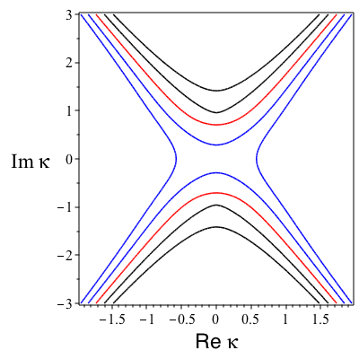
We observe that for fixed $\kappa$ and large values of $c$ the velocity of the breathers is always negative. The level set of the spectrum in the complex $\kappa$-plane corresponding to breathers with equal speed is shown in Figure 1.

Figure 1: The level set of curves of the breather speed $V$ in (1.6) in the plane $(\operatorname{Re}\kappa,\operatorname{Im}\kappa)$ for $c=1$. In black the level curves with positive velocity, in blue with negative velocity and in red the line with zero velocity. The snapshot of a breather at $t=0$ (red) and at later times in black. In the first figure $c=1,\operatorname{Re}\kappa=1,\operatorname{Im}\kappa=1.5$ and $V<0$ and in the second figure $c=1,\operatorname{Re}\kappa=0.5,\operatorname{Im}\kappa=1.5$ and $V>0$.

It has been shown in [24] that solitons and breathers on a constant background $c>0$ interact in an elastic way as in the case $c=0$. The breather (1.5) turns into a pair of soliton and antisoliton (1.4) on a constant background when we let $\chi_{1}=0$ and $\chi_{2}>0$.

For $c=0$ we have $\chi_{1}=\operatorname{Re}\kappa$ and $\chi_{2}=\operatorname{Im}\kappa$ and the solution (1.5) reduces to the standard breather [74]

$$q_{breather}(x,t;c=0,\kappa,\nu) =2\partial_{x}\arctan\left[\dfrac{(\operatorname{Im}\kappa)\cos\varphi}{(\operatorname{Re}\kappa)\cosh\Theta}\right]$$

$$=-4(\operatorname{Im}\kappa)(\operatorname{Re}\kappa)\dfrac{(\operatorname{Im}\kappa)\sinh\Theta\cos\varphi+(\operatorname{Re}\kappa)\cosh\Theta\sin\varphi}{(\operatorname{Im}\kappa)^{2}\cos^{2}(\varphi)+(\operatorname{Re}\kappa)^{2}\cosh^{2}\Theta}\,,$$

where

$$\Theta=2\operatorname{Im}\kappa\left(x+4\left(3(\operatorname{Re}\kappa)^{2}-(\operatorname{Im}\kappa)^{2}\right)t\right)+\log\dfrac{2\operatorname{Im}\kappa|\kappa|}{\operatorname{Re}\kappa|\nu|},$$

and

$$\varphi(x,t)=2\operatorname{Re}\kappa\left(x+4\left((\operatorname{Re}\kappa)^{2}-3(\operatorname{Im}\kappa)^{2}\right)t\right)+\mbox{arccos}\dfrac{-\operatorname{Im}\nu}{|\nu|}-\mbox{arccos}\dfrac{\operatorname{Re}\kappa}{|\kappa|}.$$

It has been shown in [25] that the formation of breathers is generic for certain compactly supported initial conditions.

The periodic travelling wave solution of the MKdV equation takes the form (see AppendixA)

$$\begin{split}q_{per}(x,t;\beta_{1},\beta_{2},\beta_{3},x_{0}&)=-\beta_{1}-\beta_{2}-\beta_{3}+\\ &+\frac{2(\beta_{2}+\beta_{3})(\beta_{1}+\beta_{3})}{\beta_{2}+\beta_{3}-(\beta_{2}-\beta_{1})\mathrm{cn}^{2}\left(\sqrt{\beta_{3}^{2}-\beta_{1}^{2}}(x-{\mathcal{V}}t)+x_{0}|m\right)},\end{split}$$ (1.7)

where $\beta_{3}>\beta_{2}>\beta_{1}$, the speed ${\mathcal{V}}=2(\beta_{1}^{2}+\beta_{2}^{2}+\beta_{3}^{2})$ and $x_{0}$ is an arbitrary phase. The function $\mathrm{cn}(z|m)$ is the Jacobi elliptic function of modulus

$$m^{2}=\dfrac{\beta_{2}^{2}-\beta_{1}^{2}}{\beta_{3}^{2}-\beta_{1}^{2}},$$ (1.8)

and $\mathrm{cn}(z+2K(m)|m)=-\mathrm{cn}(z|m)$ where $K(m)=\int_{0}^{\frac{\pi}{2}}\dfrac{ds}{\sqrt{1-m^{2}\sin^{2}s}}$ is the complete elliptic integral of the first kind. The periodic solution (1.7) has wave number $\mathrm{k}$, frequency $\omega$ and amplitude $a$ given by

$$\mathrm{k}=\dfrac{\pi\sqrt{\beta_{3}^{2}-\beta_{1}^{2}}}{K(m)},\quad\omega=\mathcal{V}{\mathrm{k}},\quad a=2(\beta_{2}-\beta_{1}),$$

respectively. When $m\to 1,$ the travelling wave solution (1.7) converges to the soliton solution (1.4) with $\beta_{2}=\beta_{3}=\kappa_{0}$ and $\beta_{1}=c$.

Our main result concerns the asymptotic description for large times of the MKdV initial value problem for step-like initial data of the form (1.2). Before stating our result, we remark that the description in [55] of the long-time behaviour of the solution of MKdV with the shock initial data

$$q_{0}(x)=\begin{cases}c_{+}\qquad{\rm for}\quad x>0,\\ c_{-}\qquad{\rm for}\quad x\leq 0,\end{cases}$$ (1.9)

with $c_{-}>c_{+}>0$ is as follows: there are two constant regions $\frac{x}{t}<-6c_{-}^{2}+12c_{+}^{2}-\delta$ and $\frac{x}{t}>4c_{-}^{2}+2c_{+}^{2}+\delta$ for any sufficiently small $\delta>0$, where the solution $q(x,t)=c_{\mp}+\it{o}(1)$ as $t\to\infty$ respectively. The solution that connects the two constant regions is oscillatory and it is described in terms of a genus $2$ quasi-periodic solution. In our asymptotic analysis we show that such a genus 2 solution is in fact a genus 1 solution, and can be reduced to the modulated travelling wave solution (1.7) of MKdV, namely

$$q(x,t)=q_{per}(x,t,c_{-},d,c_{+},x_{0})+O(t^{-1}),\quad-6c_{-}^{2}+12c_{+}^{2}+\delta<\frac{x}{t}<4c_{-}^{2}+2c_{+}^{2}-\delta,$$ (1.10)

where $d=d(x,t)$ depends on space and time according to

$$\dfrac{x}{t}=W_{2}(c_{+},d,c_{-}).$$ (1.11)

Here

$$W_{2}(\beta_{1},\beta_{2},\beta_{3})=2(\beta_{1}^{2}+\beta^{2}_{2}+\beta_{3}^{2})+4\dfrac{(\beta_{2}^{2}-\beta_{1}^{2})(\beta_{2}^{2}-\beta_{3}^{2})}{\beta_{2}^{2}-\beta_{3}^{2}+(\beta_{3}^{2}-\beta_{1}^{2})\frac{E(m)}{K(m)}},$$ (1.12)

with $\beta_{1}\leq\beta_{2}\leq\beta_{3}$ and $E(m)=\int_{0}^{\frac{\pi}{2}}\sqrt{1-m^{2}\sin^{2}\theta}d\theta$ the complete elliptic integral of the second kind. We have that

$$W_{2}(c_{+},c_{+},c_{-})=-6c_{-}^{2}+12c_{+}^{2}<\frac{x}{t}<4c_{-}^{2}+2c_{+}^{2}=W_{2}(c_{+},c_{-},c_{-}).$$

Figure 2: The solution of the modulated travelling wave (1.10) with $x_{0}=K(m)$, $c_{+}=0.4$, $c_{-}=0.8$ and $t=15$ (left), $t=50$ (right). We observe that the leading oscillation is approximately a soliton of maximal height $2c_{-}-c_{+}$.

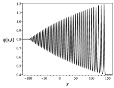
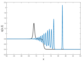
The quantity $W_{2}(\beta_{1},\beta_{2},\beta_{3})$ is the speed of the Whitham modulation equations [34] for $\beta_{1},\beta_{2}$ and $\beta_{3}$ referring to the Riemann invariants $\beta_{2}$. The solution (1.10) is the dispersive shock wave (see Figure 2) and it was first derived for the Korteweg-de Vries equation [45]. The Whitham equations for MKdV are strictly hyperbolic and genuinely nonlinear [58] only for $\beta_{2}\neq 0$ which implies that the equation (1.11) can be inverted for $d$ as a function of $\xi$ only when $c_{+}>0$. The case $c_{-}>-c_{+}>0$ can be studied in a similar way, by getting a slightly different evolution of the wave parameters (see the Appendix  B for further comments). A comprehensive set of cases arising in the long-time asymptotic solution for the MKdV equation with step initial data for various values of the parameters $c_{-}$ and $c_{+}$ has been discussed in [35, 60, 62]. The phase $x_{0}$ of the travelling wave solution (1.10) is given explicitly in terms of the scattering data associated to the MKdV equation.

We consider general step-like initial data and we subject the initial function to the following conditions.

Assumption 1.1.

The initial data $q_{0}(x)$ is assumed to be locally a function of bounded variation $BV_{loc}(\mathbb{R})$ and satisfying the following conditions

$$\int_{-\infty}^{+\infty}|x|^{2}|\mathrm{d}q_{0}(x)|<\infty$$ (1.13)

and

$$\int\limits_{\mathbb{R}^{\pm}}e^{2\sigma|x|}|q_{0}(x)-c_{\pm}|\mathrm{d}x<\infty,$$ (1.14)

where $\sigma>\sqrt{c_{-}^{2}-c_{+}^{2}}>0,$ and $\mathrm{d}q_{0}(x)$ is the corresponding signed measure (distributional derivative of $q_{0}(x)$).

This class includes the case of exact (discontinuous) step function (1.9). Note that for a function $q_{0}(x)$ which is locally of bounded variation and tends to $c_{\pm}$ as $x\to\pm\infty,$ the condition (1.13) is equivalent to

$$\int_{-\infty}^{0}(1+|x|)|q_{0}(x)-c_{-}|\mathrm{d}x+\int_{0}^{+\infty}(1+|x|)|q_{0}(x)-c_{+}|\mathrm{d}x<\infty.$$ (1.15)

Theorem 1.2.

Under Assumption 1.1, the initial value problem of the MKdV equation (1.1) has a classical solution for all $t>0$.

Under Assumption 1.1, the inverse of the transmission coefficient $a(k)$ is analytic for $k\in\mathbb{C}_{+}\setminus[\mathrm{i}c_{-},0]$, and it has continuous limits to the boundary, with the exception of the points $\mathrm{i}c_{-},$ $\mathrm{i}c_{+},$ where $a(k)$ may have at most a fourth root singularity, namely $a(k)\sqrt[4]{k-\mathrm{i}c_{\pm}}$ is bounded (see Lemma 2.3). The zeros of $a(k)$ form the point spectrum and by analiticity, the number of zeros is finite. We fix the number of zeros in the quarter plane $\operatorname{Im}k\geq 0$ and $\operatorname{Re}k\geq 0$ equal to $N$. In order to formulate our results, we enumerate the zeros of $a(k)$ in $\operatorname{Im}k\geq 0,$ $\operatorname{Re}k\geq 0$ in the decreasing order of the speed of the corresponding solitons or breathers, namely the points

$$\kappa_{1},\dots,\kappa_{N},\quad\operatorname{Im}\kappa_{j}\geq 0,\;\;\operatorname{Re}\kappa_{j}\geq 0$$

correspond to the speeds

$$+\infty>V_{1}\geq V_{2}\geq\ldots\geq V_{N}>-\infty.$$

We recall that a soliton with the point spectrum $\kappa$ on a constant background $c$ has the speed $2c^{2}+4|\kappa|^{2}$, while a breather with the point spectrum $\kappa$ on a constant background $c$ has the speed specified in (1.6). The speed of a breather on a elliptic background is specified in (4.3). In our case for each breather there are three options for large times: it travels in either the left constant background, right constant background, or dispersive shock wave background. Note that it follows from properties 11 and 12 of Lemma 2.3 below, that $a(k)$ cannot have zeros on $(\mathrm{i}c_{-},0).$ Therefore a soliton can travel only to the right of the dispersive shock vave.

We make further (generic) assumptions on the potential $q_{0}(x)$ which are formulated in terms of the associated spectral function $a(k).$

Assumption 1.3.

The spectral function $a(k)$ (see Definition 2.8) satisfies the following generic conditions:

• the zeros of $a(k)$ are simple;

• the zeros of $a(k)$ do not lie on $\mathbb{R};$

• all the speeds $V_{j}$ of breathers and solitons are distinct, namely

  $$+\infty>V_{1}>V_{2}>\ldots>V_{N}>-\infty;$$

• the behavior of $a(k)$ at the points $\mathrm{i}c_{\pm}$ is as follows: for some nonzero constants $C_{1},C_{2+},C_{2-},$

  $$\begin{split}&a(k)\sim C_{1}(k-\mathrm{i}c_{-})^{-1/4}\mbox{ as }k\to\mathrm{i}c_{-};\\ &\mbox{ in the case $c_{+}>0,$\quad}\color[rgb]{0,0,0}\definecolor[named]{pgfstrokecolor}{rgb}{0,0,0}\pgfsys@color@gray@stroke{0}\pgfsys@color@gray@fill{0}\quad a(k)\sim C_{2,\pm}(k-\mathrm{i}c_{+})^{-1/4}\mbox{ as }k\to\mathrm{i}c_{+}\pm 0,\end{split}$$

  where $k\to\mathrm{i}c_{+}\pm 0$ stands for the non tangential limit to the point $\mathrm{i}c_{+}$ from the left ($+$) and right $(-)$ side of the oriented segment $[\mathrm{i}c_{-},0]$, where the orientation is downward.

Similarly to Beals and Coifman [6], one can show that the set of potentials satisfying Assumption 1.3 form a dense open set in the space of all potentials satisfying Assumption 1.1 with respect to the topology induced by (1.15) but it is beyond the scope of this manuscript to prove this here.

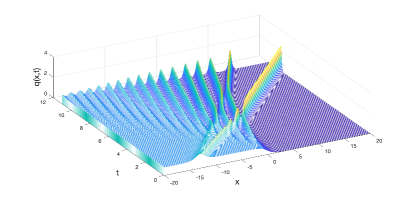
The question we address is: how, under Assumptions 1.1 and 1.3, the solitons, breathers and the dispersive shock wave interact for large values of time (see Figure 3). Theorem 1.4 characterises these interactions in the general setting and (1.17), (1.18) and (1.20) below show explicitly how these interactions affect the asymptotic phase shifts of individual solitons breathers and the dispersive shock wave.

Figure 3: The evolution into a breather with negative speed, a dispersive shock wave and a soliton (left) of a steplike initial data (right).

Now we define

$$\widetilde{T}_{j}(k)=\prod\limits_{l<j,\operatorname{Re}\kappa_{l}>0}\frac{k-\overline{\kappa}_{l}}{k-\kappa_{l}}\frac{k+\kappa_{l}}{k+\overline{\kappa}_{l}}\cdot\prod\limits_{l<j,\operatorname{Re}\kappa_{l}=0}\frac{k-\overline{\kappa}_{l}}{k-\kappa_{l}},\quad j\geq 2,\qquad\widetilde{T}_{1}(k)=1.$$ (1.16)

Theorem 1.4.

Let an initial datum satisfy Assumptions 1.1, 1.3 and let $\delta>0$ be a sufficiently small positive number such that all the breather/soliton speeds $V_{j}$ satisfy $|V_{j}-V_{l}|>4\delta$ for all $j\neq l,$ $1\leq j,l\leq N.$

Then the solution of the Cauchy problem for the MKdV equation (1.1) behaves for large $t$ in the following way:

• Soliton and breather region: $\frac{x}{t}>4c_{-}^{2}+2c_{+}^{2}+\delta_{1}$, $\delta_{1}>0$.

  For $\frac{x}{t}$ such that $|\frac{x}{t}-V_{j}|>\delta$ for all $j,$

  $$q(x,t)=c_{+}+\mathcal{O}(\mathrm{e}^{-Ct}),$$

  with some $C>0;$
  for $|\frac{x}{t}-V_{j}|<\delta$ for some $j,$

  $$q(x,t)=\left\{\begin{array}[]{ll}q_{soliton}(x,t;c_{+},\kappa_{j},x_{j})+\mathcal{O}(\mathrm{e}^{-Ct}),\quad\mbox{ if }\quad\operatorname{Re}\kappa_{j}=0,\\ &\\ q_{breather}(x,t;c_{+},\kappa_{j},\hat{\nu}_{j})+\mathcal{O}(\mathrm{e}^{-Ct}),\quad\mbox{ if }\quad\operatorname{Re}\kappa_{j}>0,\end{array}\right.$$ (1.17)

  where $q_{soliton},$ and $q_{breather}$ are defined in (1.4), (1.5) respectively and

  $$\hat{\nu}_{j}=\frac{\nu_{j}}{T_{j}^{2}(\kappa_{j})},\qquad\quad x_{j}=\ln\frac{(|\kappa_{j}|^{2}-c_{+}^{2})T_{j}^{2}(\mathrm{i}|\kappa_{j}|)}{|\nu_{j}||\kappa_{j}|}$$

  and

  $$T_{j}(k)=\widetilde{T}_{j}(k)\cdot\exp\left[\frac{\sqrt{k^{2}+c_{+}^{2}}}{2\pi\mathrm{i}}\int\limits^{\mathrm{i}c_{+}}_{-\mathrm{i}c_{+}}\frac{\ln\widetilde{T}_{j}^{2}(s)\ \mathrm{d}s}{(s-k)\left(\sqrt{s^{2}+c_{+}^{2}}\right)_{+}}\right],$$

  with $\widetilde{T}_{j}(k)$ as in (1.16) and $\left(\sqrt{s^{2}+c_{+}^{2}}\right)_{+}$ is the boundary value on the positive side of the oriented segment $[\mathrm{i}c_{+},-\mathrm{i}c_{+}]$.

• Dispersive shock wave region: $-6c_{-}^{2}+12c_{+}^{2}+\delta_{1}<\frac{x}{t}<4c_{-}^{2}+2c_{+}^{2}-\delta_{1}$, $\delta_{1}>0.$

  For $\frac{x}{t}$ such that $|\frac{x}{t}-V_{j}|>\delta$ for all $j,$ one has

  $$q(x,t)=q_{per}(x,t;c_{-},d,c_{+},x_{0})+O(t^{-1}),$$ (1.18)

  where the travelling wave $q_{per}$ has been defined in (1.7), the quantity $d=d(x,t)$ depends on $x$ and $t$ as in (1.11) and the phase

  $$x_{0}=-\dfrac{K(m)\Delta}{\pi}+K(m)$$

  depends on the discrete and continuous spectrum via the relation

  $$\begin{split}&\Delta(x,t)=-\dfrac{\sqrt{c_{-}^{2}-c_{+}^{2}}}{K(m)}\left[\int\limits^{\mathrm{i}c_{-}}_{\mathrm{i}d(x,t)}\frac{\ln(|a(s)|^{2}\widetilde{T}_{n}^{2}(s))s\mathrm{d}s}{R_{+}(s)}+\int\limits^{\mathrm{i}c_{+}}_{0}\frac{\left(\ln\widetilde{T}_{n}^{2}(s)\right)s\mathrm{d}s}{R_{+}(s)}\right]\\ &R_{+}(s)=\left(\sqrt{(s^{2}+c_{+}^{2})(s^{2}+c_{-}^{2})(s^{2}+d^{2})}\right)_{+}\end{split}$$ (1.19)

  where the quantity $\widetilde{T}_{n}(s)$ is as in (1.16), where $n=n(\frac{x}{t})$ is the number of soliton/breather speed $V_{j}$ satisfying $V_{j}>\frac{x}{t},$ and $a(k)$ is the inverse of the transmission coefficient associated to the Zakharov-Shabat spectral problem. For $\frac{x}{t}$ such that $|\frac{x}{t}-V_{j}|<\delta$ for some $j,$ one has $q(x,t)=q_{be}(x,t)+o(1)$ where $q_{be}(x,t)$ is the breather solution on the elliptic background and it is specified by the solution of the RH problem 6 in Section 4.1.2. The corresponding speed $V_{j}$ is given in (4.35).

• Breathers on a constant background: $\frac{x}{t}<-6c_{-}^{2}-\delta_{1}$ or $-6c_{-}^{2}+\delta_{1}<\frac{x}{t}<-6c_{-}^{2}+12c_{+}^{2}-\delta_{1},$ $\delta_{1}>0$.
  For $t$ large and such that $|\frac{x}{t}-V_{j}|>\delta$ for all $V_{j},$

  $$q(x,t)=c_{-}+\mathcal{O}(t^{-1/2}),$$

  and for $x/t$ such that $|\frac{x}{t}-V_{j}|<\delta$ for some $j,$

  $$q(x,t)=q_{breather}(x,t;c_{-},\kappa_{j},\hat{\nu}_{j})+\mathcal{O}(t^{-1/2}),$$ (1.20)

  where $q_{breather}$ is defined in (1.5) and the phase $\hat{\nu}_{j}$

  $$\hat{\nu}_{j}=\frac{\nu_{j}}{T_{j}^{2}(\kappa_{j},\xi)},$$

  with

  $$\begin{split}T_{j}(k,\xi)=\widetilde{T}_{j}(k)\exp&\left[\frac{-\sqrt{k^{2}+c_{-}^{2}}}{2\pi\mathrm{i}}\left\{\int\limits_{\mathrm{i}c_{-}}^{\mathrm{i}d_{0}(\xi)}-\int\limits^{-\mathrm{i}c_{-}}_{-\mathrm{i}d_{0}(\xi)}\frac{\ln|a(s)|^{2}\mathrm{d}s}{(s-k)\left(\sqrt{s^{2}+c_{-}^{2}}\right)_{+}}+\right.\right.\\ &+\left.\left.\int\limits_{\mathrm{i}c_{-}}^{-\mathrm{i}c_{-}}\frac{\left(\ln\widetilde{T}_{j}^{2}(s)\right)\mathrm{d}s}{(s-k)\left(\sqrt{s^{2}+c_{-}^{2}}\right)_{+}}\right\}\right]\end{split}$$

  for $\frac{-c_{-}^{2}}{2}<\xi<\frac{-c_{-}^{2}}{2}+c_{+}^{2}$ with $d_{0}(\xi)=\mathrm{i}\sqrt{\xi+\frac{c_{-}^{2}}{2}}$, and

  $$\begin{split}T_{j}(k,\xi)&=\widetilde{T}_{j}(k)\exp\left[\frac{-\sqrt{k^{2}+c_{-}^{2}}}{2\pi\mathrm{i}}\left\{\int\limits_{\mathrm{i}c_{-}}^{0}-\int\limits^{-\mathrm{i}c_{-}}_{0}\frac{\ln|a(s)|^{2}\mathrm{d}s}{(s-k)\left(\sqrt{s^{2}+c_{-}^{2}}\right)_{+}}\right.\right.\\ &\left.\left.+\int\limits_{\mathrm{i}c_{-}}^{-\mathrm{i}c_{-}}\frac{\ln\widetilde{T}_{j}^{2}(s)\mathrm{d}s}{(s-k)\left(\sqrt{s^{2}+c_{-}^{2}}\right)_{+}}-\int\limits_{-k_{0}(\xi)}^{k_{0}(\xi)}\frac{\ln\left(1+|r(s)|^{2}\right)\mathrm{d}s}{(s-k)\sqrt{s^{2}+c_{-}^{2}}}\right\}\right],\end{split}$$

  for $\xi<-\frac{c_{-}^{2}}{2}$ and $\color[rgb]{0,0,0}\definecolor[named]{pgfstrokecolor}{rgb}{0,0,0}\pgfsys@color@gray@stroke{0}\pgfsys@color@gray@fill{0}{k_{0}}(\xi)=\sqrt{-\xi-\frac{c_{-}^{2}}{2}}$ and $\widetilde{T}_{j}(k)$ as in (1.16).

The subleading term of order ${\mathcal{O}}(t^{-\frac{1}{2}})$ of the expansion of $q(x,t)$ as $t\to\infty$ in the left constant region is oscillatory and is described by the theorem below.

Theorem 1.5.

Away from breathers, the subleading term of the expansion of $q(x,t)$ as $t\to\infty$ in the regions $x<(-6c_{-}^{2}-\delta_{1})t$ and $(-6c_{-}^{2}+\delta_{1})t<x<(-6c_{-}^{2}+12c_{+}^{2}-\delta_{1})t$ is given by the formula

$$\begin{split}q(x,t)&=c_{-}+\sqrt{\frac{|\nu(\xi)|\sqrt{-\xi+\frac{c_{-}^{2}}{2}}}{3t\,|\xi+\frac{c_{-}^{2}}{2}|}}\times\\ &\times\cos\left[16t\left(-\xi+\frac{c_{-}^{2}}{2}\right)^{\frac{3}{2}}+\nu(\xi)\ln\left(\frac{192\,t\,(\xi+\frac{c_{-}^{2}}{2})^{2}}{\sqrt{-\xi+\frac{c_{-}^{2}}{2}}}\right)+\phi(\xi)\right]+\mathcal{O}(t^{-1}),\end{split}$$ (1.21)

where $\xi=\frac{x}{12t}$ and the phase shift and parameter $\nu(\xi)$ are different for different regions of $\xi=\frac{x}{12t}:$
$\bullet$ for $\xi<-\frac{c_{-}^{2}}{2}$ they are given by the formulas

$$\begin{split}&\nu(\xi)=\frac{1}{2\pi}\ln(1+|r(k_{0})|^{2}),\quad k_{0}=\sqrt{-\xi-\frac{c_{-}^{2}}{2}},\\ &\phi(\xi):=\frac{\pi}{4}-\arg r(k_{0})-\arg\Gamma(\mathrm{i}\nu(\xi))+\arg\chi^{2}(k_{0}),\end{split}$$ (1.22)

and $\chi(k_{0})=\lim\limits_{k\to k_{0}}T(k)\left(\frac{k-k_{0}}{k+k_{0}}\right)^{\mathrm{i}\nu(\xi)},$
$\bullet$ and for $-\frac{c_{-}^{2}}{2}<\xi<-\frac{c_{-}^{2}}{2}+c_{+}^{2}$ they are given by the formulas

$$\begin{split}&\nu(\xi)=\frac{1}{2\pi}\ln(1-|r_{+}(\mathrm{i}d_{0})|^{2})<0,\quad\mathrm{i}d_{0}=\mathrm{i}\sqrt{\xi+\frac{c_{-}^{2}}{2}},\\ &\phi(\xi)=-\frac{\pi}{4}-\arg r_{+}(\mathrm{i}d_{0})-\arg\Gamma(\mathrm{i}\nu(\xi))+\arg\chi^{2}(\mathrm{i}d_{0}),\end{split}$$ (1.23)

and $\chi(\mathrm{i}d_{0})=\lim\limits_{k\to\mathrm{i}d_{0}+0}T(k)\left(\frac{k-\mathrm{i}d_{0}}{-(k+\mathrm{i}d_{0})}\right)^{\mathrm{i}\nu(\xi)},$ $\quad|\chi(\mathrm{i}d_{0})|=1.$

Remark 1.6.

Note that the term $\frac{\pi}{4}$ in the phase shifts has different signs for different values of $\xi,$ and that the parameter $\nu(\xi)$ has different signs in different regions. We also observe that the amplitude in the formula (1.21) does not blow up when $\xi$ approaches $-\frac{c_{-}^{2}}{2}$ if $c_{+}>0,$ since $\nu(\xi)$ has a first order zero as $\xi=-\frac{c_{-}^{2}}{2}$ for $c_{+}>0$ while it blows up at $c_{+}=0$. This suggests the existence of a non trivial transition zone.

Our analysis is obtained by formulating the inverse scattering problem for the MKdV equation with step initial data as a RH problem and then we implement the long-time asymptotic analysis via the Deift-Zhou steepest descent method [31]. The proof that the oscillations in the oscillatory region that were obtained in [55] via genus two theta functions, can be reduced to the dispersive shock wave solution for the MKdV equation, is obtained by “folding” the genus two Riemann Hilbert problem to a genus one RH problem with poles. Further analysis permits us to get rid of the poles and to reduce the solution to the travelling wave solution of the MKdV equation. The estimate of the errors and the calculation of the subleading terms of the expansion in Theorems 1.4 and Theorem 1.5 is obtained via the construction of local parametrices in terms of Airy functions and parabolic cylinder functions.

We illustrate our results with the following examples.

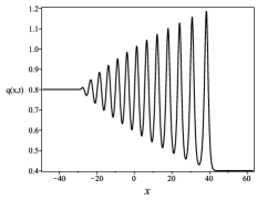
Example 1.7.

For the exact step (1.9) one has that the reflection coefficient and the inverse of the transmission coefficients are [55, formula (3.3)]

$$r(k)=\dfrac{\gamma(k)^{2}-1}{\gamma(k)^{2}+1},\quad a(k)=\frac{1}{2}\left(\gamma(k)+\frac{1}{\gamma(k)}\right),\ \gamma(k)=\left(\dfrac{(k-\mathrm{i}c_{-})(k+\mathrm{i}c_{+})}{(k+\mathrm{i}c_{-})(k-\mathrm{i}c_{+})}\right)^{\frac{1}{4}}\,.$$

The dispersive shock wave is given by the relation (1.18) with phase shift

$$x_{0}=-\dfrac{\sqrt{c_{-}^{2}-c_{+}^{2}}}{\pi}\int\limits^{\mathrm{i}c_{-}}_{\mathrm{i}d(x,t)}\frac{\ln(|a(s)|^{2})s\mathrm{d}s}{\sqrt{(s^{2}+c_{+}^{2})(s^{2}+c_{-}^{2})(s^{2}+d^{2})}}+K(m)\,,$$

The evolution for such initial data is illustrated in Figure 4. The leading edge of the oscillatory region has been studied in [53], where it has been identified with a train of asymptotic solitons, and it has been shown that the amplitude of the first soliton is approximately described

$$q(x,t)\simeq q_{soliton}(x,t;c_{+},c_{-},\tilde{x}_{0})$$

where $\tilde{x}_{0}=\frac{3}{2}\log t+\alpha$ for some constant $\alpha$. Here $q_{soliton}(x,t;c_{+},c_{-},\tilde{x}_{0})$ is the soliton solution (1.4) on the constant background $c_{+}$ with spectrum $c_{-}$. The highest peak of the first soliton is approximately located at the position $x_{s}(t)=2(c_{+}^{2}+2c_{-}^{2})t-\frac{1}{2}\frac{\frac{3}{2}\log t+\alpha}{\sqrt{c_{-}^{2}-c_{+}^{2}}}$. The transition region between the dispersive shock wave and asymptotic solitons turned out to be very rich, and has been studied recently in [7].

Figure 4: The (smoothed) step initial data (1.9) in black for $c_{-}=0.8$ and $c_{+}=0.4$. The blue line shows the evolution at time $t=15$.

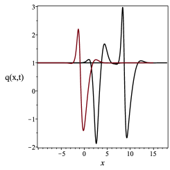
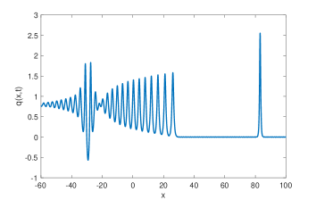
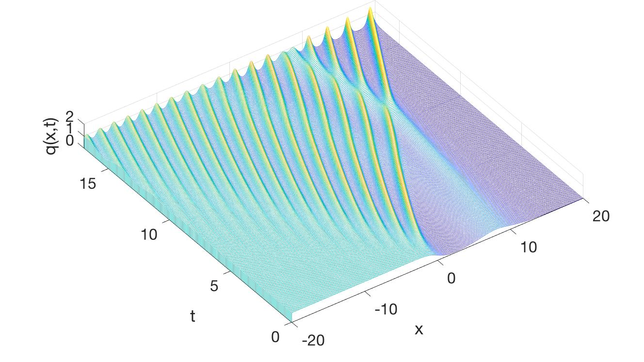
Example 1.8.

For an initial function in the form of a soliton on a constant background (1.4) on the left, and a constant on the right, i.e.

$$q_{0}(x)=\begin{cases}q_{soliton}(x,0;c_{-},\kappa_{0},x_{0}),\quad x<0,\qquad\mbox{ where }\quad\kappa_{0}>c_{-}>0,\\ c_{+},\quad x>0,\quad\mbox{where }c_{+}\in\mathbb{R}.\end{cases}$$

Here $x_{0}=\log\dfrac{2(\kappa_{0}^{2}-c_{-}^{2})}{|\nu|\kappa_{0}}\in\mathbb{R}$ and $\nu\neq 0$.

The evolution is shown in Figure 5, where it is shown that the initial approximate ”soliton” decomposes in two solitons that pass rapidly through the dispersive shock wave.

Figure 5: The (smoothed) initial data of Example 1.8 for $c_{-}=0.8$ and $c_{+}=0.4$, $\kappa_{0}=1$ and $x_{0}=10$, and $\nu>0$. On the left figure the evolution of $q(x,t)$ in the $(x,t)$ plane. On the right figure, the black line shows the initial data and the blue line the evolution at time $t=11$.

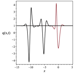
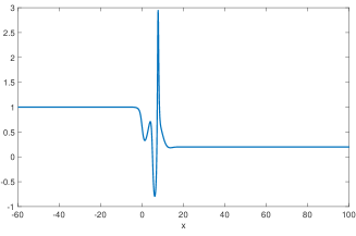
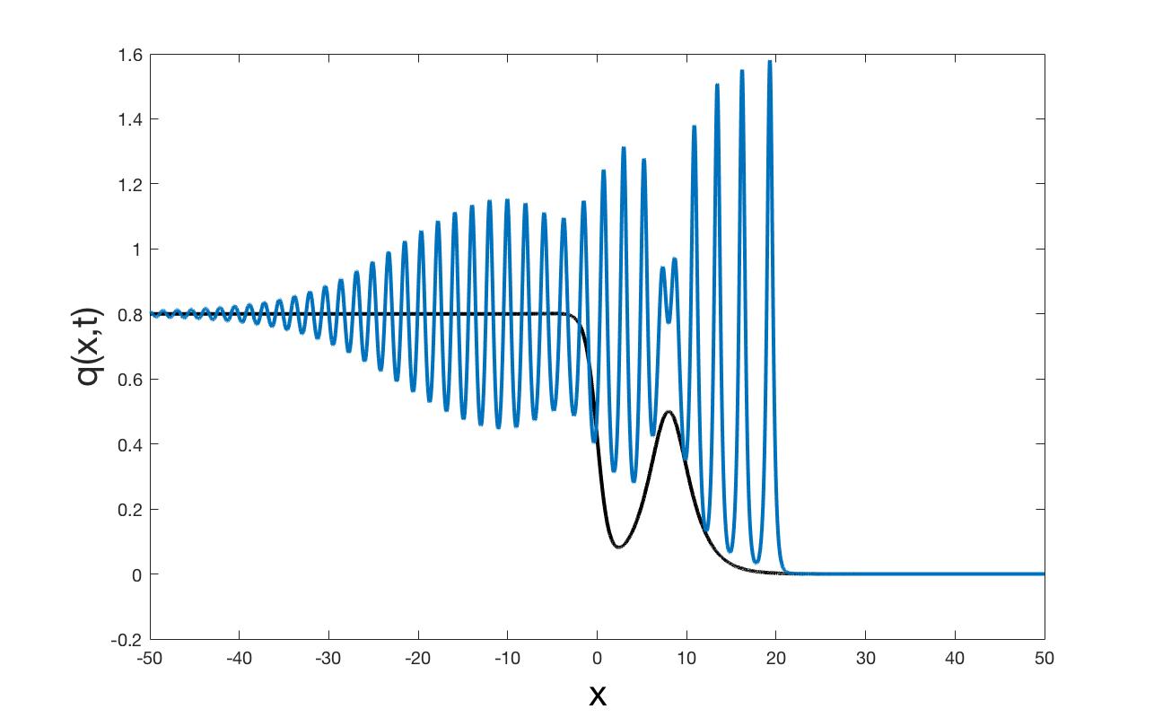
Example 1.9.

Consider the initial function in the form of a constant $c>0$ on the left, and a soliton on a zero background on the right, i.e.

$$q_{0}(x)=\begin{cases}c>0,\quad x<0,\\ \frac{-2\kappa_{0}\mathrm{sgn}(\nu)}{\cosh\left[2\kappa_{0}(x-x_{0})\right]},\quad x>0,\quad\nu\in\mathbb{R}\setminus\left\{0\right\},\ c>\kappa_{0}>0,\quad x_{0}=\frac{1}{2\kappa_{0}}\ln\left|\frac{\nu}{2\kappa_{0}}\right|.\end{cases}$$ (1.24)

This initial data does not satisfy the decay at infinity of Assumption 1.1. Below we show that the reflection coefficient is singular on the imaginary axis $[\mathrm{i}c,0]$. The reflection coefficient is $r(k)=\frac{b(k)}{a(k)}$ with

$$\begin{split}&a(k)=\frac{1}{2}\left[\left(\gamma(k)+\gamma(k)^{-1}\right)\left(1-\frac{\mathrm{i}\alpha}{k+\mathrm{i}\kappa_{0}}\right)-\left(\gamma(k)-\gamma(k)^{-1}\right)\frac{\mathrm{i}\beta}{k+\mathrm{i}\kappa_{0}}\right],\\ &b(k)=\frac{1}{2}\left[\left(\gamma(k)-\gamma(k)^{-1}\right)\left(1+\frac{\mathrm{i}\alpha}{k-\mathrm{i}\kappa_{0}}\right)-\left(\gamma(k)+\gamma(k)^{-1}\right)\frac{\mathrm{i}\beta}{k-\mathrm{i}\kappa_{0}}\right],\end{split}$$

where

$$\gamma(k)=\sqrt[4]{\frac{k-\mathrm{i}c}{k+\mathrm{i}c}},\quad\alpha=\frac{2\nu^{2}\kappa_{0}}{4\kappa_{0}^{2}+\nu^{2}},\quad\beta=\frac{4\nu\kappa_{0}^{2}}{4\kappa_{0}^{2}+\nu^{2}}.$$

The coefficient $b(k)$ has a pole at $k=\mathrm{i}\kappa_{0}$ and the function $a(k)$ has two zeros $k_{1},k_{2}$ in the half-plane $\operatorname{Im}k\geq 0$ :

$$k_{1,2}=\dfrac{\pm\beta\sqrt{c^{2}+2c\beta-(\alpha-\kappa_{0})^{2}}+\mathrm{i}(\alpha-\kappa_{0})(\beta+c)}{c+2\beta}$$

and they are symmetric w.r.t. imaginary axis: $k_{1}=-\overline{k_{2}}.$ Let us notice that when $x_{0}>0$ is not small, and hence $\nu>0$ is big, we have $\alpha\sim 2\kappa_{0},$ $\beta\sim 0,$ and hence

$$k_{1,2}\sim\pm 0+\mathrm{i}\kappa_{0}.$$

Therefore the soliton part of the initial data is a breather from the spectral point of view, with point spectrum very close to the imaginary axis. The velocity of the breather is approximately $4\kappa_{0}^{2}<4c^{2}$ while the velocity of the dispersive shock wave is $-6c^{2}<\frac{x}{t}<4c^{2}$. Namely the breather has a positive velocity that is smaller then the velocity of the leading front of the dispersive shock wave and it will remain trapped by the dispersive shock wave. Furthermore, since $b(k)$ has a pole at $k=\mathrm{i}\kappa_{0},$ also the reflection coefficient has a pole at $k=\mathrm{i}\kappa_{0}$, and this pole requires a quite delicate asymptotic analysis that is beyond the scope of the present article. In the physical literature [71] this phenomenon received the name of ‘soliton trapping’ inside the dispersive shock wave (see Figure 6).

Figure 6: The initial data (1.24) for $c_{-}=0.8$ and $c_{+}=0.0$, $\kappa_{0}=0.25$. On the left, the 2D plot in the $(x,t)$ plane. On the right figure, the black line shows the initial data, while the blue line the evolution at time $t=17$.

This manuscript is organized as follow. We study the direct scattering problem and the main properties of the scattering data and the solvability of the associated RH problem in section 2. In section 3 we formulate and solve the RH problems associated to the model problems that will be used in asymptotic analysis, namely the RH problem for a breather and a soliton on a constant background and then the model problems for the periodic solution that is expressed via hyperelliptic curves. We will then show how to reduce the hyperelliptic solution to a travelling wave solution of MKdV.

In section 4 we start the asymptotic analysis introducing the $g$-function and performing the contour deformation and asymptotic analysis in the elliptic region and in section 5 we perform the contour deformation and asymptotic analysis in the left and right constant regions, to arrive at our main result, namely the proof of theorem 1.4. In section 6 we calculate the subleading order correction of the left constant region thus proving theorem 1.5. Several appendices are used to prove the most technical results.

2 Preliminaries

Let us briefly describe what will happen in this Section.

In section 2.1 we review the Lax pair formulation of the MKdV equation and we construct the Jost solutions at time $t=0$. In section 2.2 we analyze the direct scattering problem following and extending the derivation in [54] for our class of initial data. In Section 2.3 we introduce the RH problem 1, where we imposed a time dependence of the form $e^{i4k^{3}t}.$ The way we arrive to the RH problem 1 is heuristic, nevertheless, after the RH problem 1 is stated, it serves as a basis for the rest of the section. In Section 2.4 we follow [56] and, first, we prove that the solution of the RH problem exists and admits differentiation with respect to the parameters $x,t,$ and, second, that the columns of the solution of the RH problem 1 are solutions of the overdetermined system which constitutes the Lax pair (2.1), (2.2). This allows to define a function $q(x,t),$ which satisfies the MKdV equation (1.1) and equals to the initial datum at $t=0.$

Note that the existence of RH problem’s solution is guaranteed a priori by the Zhou’s Schwartz reflection argument [78], but in order to guarantee the differentiability in the parameters $x,t$ we need either to require analytic continuation of the reflection coefficient off the real axis, or to require sufficiently fast decay of the reflection coefficient at the infinite parts of the RH problem’s contour. The former can be achieved by imposing the exponential decay (1.14), and the latter by requiring sufficient smoothness of the initial function. Neither of these function spaces is embedded in each other, but we chose to impose the exponential decay of the initial datum rather than the smoothness condition. This allows us to treat the important cases of discontinuous initial functions described in Examples (1.7)-(1.8).

Remark 2.1.

Results similar to that of Theorem 1.5 but written for large $x\to-\infty$ and fixed $t$ allow to conclude that $|q(x,t)|\sim\frac{|r(-\frac{x}{12t})|}{\sqrt[4]{x}}\sim|x|^{-\frac{j}{2}-\frac{3}{4}}$ for an initial datum $q(x,0)$ whose $j$-th derivative is locally a function of bounded variation. In the above the symbol $\sim$ means of the same order. Thus, the function $q(x,t)$ at a later time $t>0$ satisfies the first moment condition (1.15) only when $j\geq 3,$ which is a much stronger condition than the conditions set in Assumption 1.1. Note that the classical direct analysis of the $x-$equation (2.1) allows to guarantee the existence of the Jost solutions only under the convergence of the first moment (1.15).

2.1 Lax pair and Jost solutions

The MKdV equation (1.1) admits the Lax pair representation in the form of an over-determined system of linear ordinary equations for a $2\times 2$ matrix-valued function $\Phi(x,t;k),$ where $k\in\mathbb{C}$ is the spectral variable [73],

$$\Phi_{x}(x,t;k)=(-\mathrm{i}k\sigma_{3}+Q(x,t))\Phi(x,t;k),$$ (2.1)

$$\Phi_{t}(x,t;k)=(-4\mathrm{i}k^{3}\sigma_{3}+\widehat{Q}(x,t;k))\Phi(x,t;k),$$ (2.2)

where $\Phi_{x}$ and $\Phi_{t}$ stand for partial derivative with respect to $x$ and $t$ respectively, $\sigma_{3}=\begin{pmatrix}1&0\\ 0&-1\end{pmatrix}$ and

$$Q(x,t)=\begin{pmatrix}0&q(x,t)\\ -q(x,t)&0\end{pmatrix},\quad\widehat{Q}(x,t;k)=4k^{2}Q-2\mathrm{i}k(Q^{2}+Q_{x})\sigma_{3}+2Q^{3}-Q_{xx}.$$ (2.3)

The compatibility condition $\Phi_{xt}=\Phi_{tx}$ is equivalent to the MKdV equation. If we substitute $q(x,t)=c$ (constant) in (2.3), then the Lax pair equations (2.1), (2.2) admit explicit solutions [54, page 3]

$$E_{0}(x,t;k)=\mathrm{e}^{-(ikx+4ik^{3}t)\sigma_{3}},$$

for $c=0$ and

$$\begin{split}E_{c}(x,t;k)&=\dfrac{1}{2}\begin{pmatrix}\gamma(k)+\gamma^{-1}(k)&\gamma(k)-\gamma^{-1}(k)\\ \gamma(k)-\gamma^{-1}(k)&\gamma(k)+\gamma^{-1}(k)\end{pmatrix}\mathrm{e}^{-g_{c}(x,t;k)\sigma_{3}},\quad\\ \mbox{ where }&\gamma(k)=\sqrt[4]{\frac{k-\mathrm{i}c}{k+\mathrm{i}c}},\quad g_{c}(x,t;k)=\mathrm{i}(x+2t(2k^{2}-c^{2})\sqrt{k^{2}+c^{2}},\end{split}$$ (2.4)

for $c\neq 0;$ the root functions are defined in such a way that they have branch cut across the interval $[\mathrm{i}c,-\mathrm{i}c].$ In particular $\sqrt{k^{2}+c^{2}}$ is real for $k\in\mathbb{R}\cup[\mathrm{i}c,-\mathrm{i}c]$ and positive for $k=0+$ where $0+$ means the non tangential limit from the right with respect to the imaginary axis. Here and in the rest of the manuscript the imaginary axis is oriented downwards and for this reason we use the notation $[\mathrm{i}c,-\mathrm{i}c]$ for the oriented segment with endpoints $\pm\mathrm{i}c_{-}$.

2.2 Direct scattering

Below we give a quick review of the direct scattering problem for step-like initial data $q(x,0)$ (1.2).

We denote $E^{+}(x;k)\equiv E_{c_{+}}(x,0;k)$ and $E^{-}(x;k)\equiv E_{c_{-}}(x,0;k)$ where $E_{c_{\pm}}(x,t;k)$ is the matrix defined (2.4). Now we consider equation (2.1) for $t=0$ and define the Jost solutions $\Phi^{\pm}(x;k):=\Phi^{\pm}(x,0;k),$ which satisfy the equation (2.1), and have the (defining) property that

$$\Phi^{\pm}(x;k)=E^{\pm}(x;k)(1+o(1))\quad\mbox{as $x\to\pm\infty$},\;\;\color[rgb]{0,0,0}\definecolor[named]{pgfstrokecolor}{rgb}{0,0,0}\pgfsys@color@gray@stroke{0}\pgfsys@color@gray@fill{0}{k\in\mathbb{R}\cup[\mathrm{i}c_{\pm},-\mathrm{i}c_{\pm}].}$$ (2.5)

The Jost solutions have the following integral representation

$$\Phi^{\pm}(x;k)=E^{\pm}(x;k)+\int^{x}_{\pm\infty}L^{\pm}(x,y)E^{\pm}(y;k)dy,$$ (2.6)

where the kernels $L^{\pm}(x,y)$ are independent from $k$ and they are studied in the Appendix C. From the above expression it is clear that the Jost functions are continuous in the variable $k$ for $k\in\mathbb{R}\cup(\mathrm{i}c_{\pm},-\mathrm{i}c_{\pm}).$ The following two Lemmas appeared before in [54, section II], [55, section 2] under the condition $c_{+}=0$ or $c_{+}>0$ for the exact step, ( see also [5]) but their proof was skipped there.

Lemma 2.2.

Suppose the the initial data $q(x,0)$ satisfies Assumption 1.1 and Assumption 1.3. Then the Jost solutions (2.6) their columns $\Phi^{\pm}_{j}(x;k)$, $j=1,2$ and their entries $\Phi^{\pm}_{ij}(x;k)$ have the following properties.

1. $\det\Phi^{\pm}(x;k)=1$.

2. $\Phi_{1}^{+}(x;k)$ is analytic in $k\in\mathbb{C}^{-}\setminus[0,-\mathrm{i}c_{+}]$, and continuous up to the boundary
   $\Phi_{2}^{+}(x;k)$ is analytic in $k\in\mathbb{C}^{+}\setminus[\mathrm{i}c_{+},0]$ and continuous up to the boundary,
   $\Phi_{1}^{-}(x;k)$ is analytic in $k\in\mathbb{C}^{+}\setminus[\mathrm{i}c_{-},0]$ and continuous up to the boundary
   $\Phi_{2}^{-}(x;k)$ is analytic in $k\in\mathbb{C}^{-}\setminus[0,-\mathrm{i}c_{-}]$ and continuous up to the boundary.
    here $\mathbb{C}^{\pm}=\left\{k:\ \pm\operatorname{Im}k>0\right\};$

3. Let $\Phi(x;k)$ denote either $\Phi^{-}(x;k)$ or $\Phi^{+}(x;k)$. By the reality of $q(x)$ we have the symmetries:

   $$\begin{split}\overline{\Phi_{1}(x;\overline{k})}&=\begin{pmatrix}0&1\\ -1&0\end{pmatrix}\Phi_{2}(x;k),\\ \Phi_{1}(x;-k)&=\begin{pmatrix}0&1\\ -1&0\end{pmatrix}\Phi_{2}(x;k),\\ \overline{\Phi(x;-\overline{k})}&=\Phi(x,k).\end{split}$$

4. Large $k$ asymptotics:

   $$\begin{pmatrix}\Phi^{+}_{1}(x;k)e^{+ikx},&\Phi^{-}_{2}(x;k)e^{-ikx}\end{pmatrix}=I+{\mathrm{O}}\left(\displaystyle\frac{1}{k}\right),\quad k\rightarrow\infty,\quad\operatorname{Im}k\leq 0,$$

   $$\begin{pmatrix}\Phi^{-}_{1}(x;k)e^{+ikx},&\Phi^{+}_{2}(x;k)e^{-ikx}\end{pmatrix}=I+{\mathrm{O}}\left(\displaystyle\frac{1}{k}\right),\quad k\rightarrow\infty,\quad\operatorname{Im}k\geq 0,$$

   where $I$ stands for the $2\times 2$ identity matrix.

5. Jump conditions:
   $\Phi_{-}(x;k)=\Phi_{+}(x;k)\left(\begin{array}[]{ccc}0&i\\ i&0\end{array}\right),\quad k\in(\mathrm{i}c,-\mathrm{i}c)$,
   where $\Phi(x;k)$ and $c$ denote $\Phi^{-}(x;k)$ and $c_{-}$ or $\Phi^{\mathfrak{+}}(x;k)$ and $c_{{+}}$, respectively, and $\Phi_{\pm}(x;k)$ denotes the non-tangential limits of the matrix $\Phi(x;k)$ from the left ($+$) and from the right ($-$) of the segment $(\mathrm{i}c,-\mathrm{i}c)$ which is oriented from $\mathrm{i}c$ to $-\mathrm{i}c$ (i.e., $\Phi_{\pm}(x;k)=\lim\limits_{\epsilon\to+0}\Phi(x;k\pm\epsilon)$).

Proof.

The full proof of the Lemma is given in the Appendix C. Here we will only prove properties 1, 3 and 5.
Property 1. The functions $\Phi^{\pm}$ satisfy the $x-$equation (2.1) for $t=0$; since the trace of the function $-\mathrm{i}k\sigma_{3}+Q$ equals 0, by Liouville’s formula for determinants, it follows that $\det\Phi^{\pm}(x;k)$ are independent of $x.$ From the large $x$ asymptotics (2.5) we then obtain that the determinants are equal to $1.$
Property 3. Let us write the $x-$equation (2.1) element-wise,

$$\begin{split}&\begin{cases}\Phi_{11,x}(x;k)+\mathrm{i}k\Phi_{11}(x;k)=q(x)\Phi_{21}(x;k),\\ \Phi_{21,x}(x;k)-\mathrm{i}k\Phi_{21}(x;k)=-q(x)\Phi_{11}(x;k),\end{cases}\\ &\begin{cases}\Phi_{12,x}(x;k)+\mathrm{i}k\Phi_{12}(x;k)=q(x)\Phi_{22}(x;k),\\ \Phi_{22,x}(x;k)-\mathrm{i}k\Phi_{22}(x;k)=-q(x)\Phi_{12}(x;k).\end{cases}\end{split}$$

Changing in the last two equations $k\to-k$ and using the large $x$-asymptotics of $\Phi_{ij},i,j=1,2$, we get that $\Phi_{12}(x;-k)=-\Phi_{21}(x;k),\quad\Phi_{11}(x;k)=\Phi_{22}(x;-k)$ and $\Phi_{ij}(x;-\overline{k})=\overline{\Phi_{ij}(x;k)},\ i,j=1,2.$
Indeed, the two pairs of vector-valued functions, $(\Phi_{22}(x;-k),-\Phi_{12}(x;-k))$ and
$(\overline{\Phi_{11}(x;-\overline{k})},\overline{\Phi_{21}(x;-\overline{k})})$ satisfy the same systems of equations as $(\Phi_{11}(x;k),\Phi_{21}(x;k))$ and the same large $x$ asymptotics, and hence coincide with the latter.
Property 5. We use the defining property (2.5) of the functions $\Phi^{\pm}$ and note that the limiting values of $E^{\pm}$ on the two sides of the oriented interval $(\mathrm{i}c_{\pm},-\mathrm{i}c_{\pm})$ satisfy $E^{\pm}_{-}(x;k)=E^{\pm}_{+}(x;k)\begin{pmatrix}0&\mathrm{i}\\ \mathrm{i}&0\end{pmatrix}.$ Thus, both functions $\Phi^{\pm}_{-}(x;k)$ and $\Phi^{\pm}_{+}(x;k+0)\begin{pmatrix}0&\mathrm{i}\\ \mathrm{i}&0\end{pmatrix}$ satisfy the same differential equation (2.1) (at $t=0$), and the same asymptotics as $x\to-\infty,$ and thus they are equal.

∎

Since the matrix-valued functions $\Phi^{\pm}(x;k)$ are solutions of the first order differential equation (2.1), they are linearly dependent, i.e. there exists an $x$-independent transition matrix $T(k)$, such that

$$T(k)=(\Phi^{{+}}(x;k))^{-1}\Phi^{{-}}(x;k),\quad k\in\mathbb{R}\cup(\mathrm{i}c_{+},-\mathrm{i}c_{+}).$$ (2.7)

Due to symmetries of the $x$-equation (2.1) the transition matrix has the following structure:

$$T(k)=\begin{pmatrix}a(k)&-\overline{b(\overline{k})}\\ b(k)&\overline{a(\overline{k})}\end{pmatrix},\qquad a(k)=\det\left(\Phi^{-}_{1},\Phi^{+}_{2}\right),\ b(k)=\det\left(\Phi^{+}_{1},\Phi^{-}_{1}\right).$$ (2.8)

Note that the representation (2.8) and Lemma 2.2 allow to extend the domains of definition of the spectral functions $a,b$: the function $a(k)$ is analytic for $k\in\mathbb{C}\setminus[\mathrm{i}c_{-},0],$ and is defined also on both sides of the interval $(0,-\mathrm{i}c_{+})$, and $b(k)$ is defined for $k\in\mathbb{R}\cup(\mathrm{i}c_{+},-\mathrm{i}c_{-}).$
By property 1 of Lemma 2.2, we have that $\det T(k)=1$ so that

$$a(k)\overline{a(\overline{k})}+b(k)\overline{b(\overline{k})}=1.$$ (2.9)

The functions $a^{-1}(k)$ and

$$r(k):=\frac{b(k)}{a(k)},\quad k\in\mathbb{R}\cup(\mathrm{i}c_{+},-\mathrm{i}c_{+})$$

are called the (right) transmission and reflection coefficients, respectively. Below we sumarize the analytical properties of the functions $a(k)$, $b(k)$ and $r(k)$. We denote by $a_{\pm}(k)$, $b_{\pm}(k)$ and $r_{\pm}(k)$ the non-tangential limits of $a(k)$, $b(k)$ and $r(k)$ from the left ($+$) and from the right ($-$) of the segment $(\mathrm{i}c_{-},-\mathrm{i}c_{-})$ which is oriented from $\mathrm{i}c_{-}$ to $-\mathrm{i}c_{-}.$

Lemma 2.3.

Suppose that the initial data $q(x,0)$ satisfies Assumption 1.1 and Assumption 1.3. Then the spectral functions $a(k),b(k),r(k)$ have the following properties enumerated below.

1. Analyticity:
   $a(k)$ is analytic for $k\in\mathbb{C}^{+}\setminus[\mathrm{i}c_{-},0]$, and it can be extended continuously up to the boundary, with the exception of the points $\mathrm{i}c_{-},$ $\mathrm{i}c_{+},$ where $a(k)$ may have at most a fourth root singularity $(k-\mathrm{i}c_{\pm})^{-1/4}$ (i.e. the function $a(k)(k-\mathrm{i}c_{\pm})^{1/4}$ is bounded as $k\to\mathrm{i}c_{\pm}$). The function $a(k)$ might have at most a finite number of zeros for $k\in\mathbb{C}_{+}\setminus[\mathrm{i}c_{-},0]$.
   The function $b(k)$ is defined for $k\in\mathbb{R}\cup(\mathrm{i}c_{{+}},-\mathrm{i}c_{+})$. The function $r(k)$ is defined for $k\in\mathbb{R}\cup(\mathrm{i}c_{{+}},-\mathrm{i}c_{{+}})$ except for the points where $a(k)=0$.
   Under the condtion (1.14), the function $a(k)$ and $b(k)$ have an analytic extension in the $\delta-$neighborhood of $\Sigma=\mathbb{R}\cup[\mathrm{i}c_{-},-\mathrm{i}c_{-}]$, where $\delta=\sqrt{\sigma^{2}+c_{+}^{2}}-c_{-}$ and $\sigma>\sqrt{c_{-}^{2}-c_{+}^{2}}>0$, with $\sigma$ as in Assumptions 1.1. The function $r(k)$ is meromorphic in the same domain with poles at the zeros of $a(k).$

2. Asymptotics:
   

   $$\begin{split}&a(k)=1+\mathcal{O}(k^{-1})\quad\textrm{ as }\quad k\to\infty,\operatorname{Im}k\geq 0;\\ &r(k)=\mathcal{O}(k^{-1}).\end{split}$$

3. Symmetries: in their domains of definition

   $$\overline{a\left(-\overline{k}\right)}=a(k),\quad\overline{b\left(-\overline{k}\right)}=b(k),\quad\overline{r\left(-\overline{k}\right)}=r(k).$$

4. On $(\mathrm{i}c_{+},-\mathrm{i}c_{+}):$
   

   $$a_{-}(k)=\overline{a_{+}\left(\overline{k}\right)},\quad b_{-}(k)=-\overline{b_{+}\left(\overline{k}\right)},\quad r_{-}(k)=-\overline{r_{+}\left(\overline{k}\right)},$$

   and on $\color[rgb]{0,0,0}\definecolor[named]{pgfstrokecolor}{rgb}{0,0,0}\pgfsys@color@gray@stroke{0}\pgfsys@color@gray@fill{0}{(\mathrm{i}c_{-},\mathrm{i}c_{+})}:$

   $$a_{-}(k)=-\mathrm{i}\ \overline{b_{+}\left(\overline{k}\right)},\quad a_{+}(k)=\mathrm{i}\ \overline{b_{-}\left(\overline{k}\right)}.$$

5. Let

   $$f(k):=\displaystyle\frac{i}{a_{-}(k)a_{+}(k)},\quad k\in(\mathrm{i}c_{{-}},0),$$

   then on $(\mathrm{i}c_{-},\mathrm{i}c_{+}):$

   $$f(k)=\frac{\mathrm{i}}{a_{-}(k)a_{+}(k)}=r_{-}(k)-r_{+}(k)=\frac{-1}{a_{+}(k)\overline{b_{+}\left(\overline{k}\right)}}=\frac{1}{a_{-}(k)\overline{b_{-}\left(\overline{k}\right)}},$$

   and on $(\mathrm{i}c_{+},0):$

   $$f(k)=\frac{\mathrm{i}}{a_{-}(k)a_{+}(k)}=\mathrm{i}(1-r_{-}(k)r_{+}(k)).$$

1. If $c_{+}>0,$ then $|a(0)|=1,$ and $|a(k)|\leq 1$ for $k\in\mathbb{R}\setminus\left\{0\right\}$ and $|a(k)|\geq 1$ for $k\in(\mathrm{i}c_{+},0).$

2. Nonvanishing. The coefficients $a(k)$ and $\overline{b(\overline{k})}$ do not vanish on the segment $(\mathrm{i}c_{-},\mathrm{i}c_{+});$

3. $\displaystyle\frac{(\Phi^{-}_{1}(x;k))_{-}}{a_{-}(k)}-\displaystyle\frac{(\Phi^{-}_{1}(x;k))_{+}}{a_{+}(k)}=f(k)\Phi^{+}_{2}(x;k),\quad k\in(\mathrm{i}c_{{-}},\mathrm{i}c_{{+}}),$
   and $\displaystyle\frac{(\Phi^{-}_{2}(x;k))_{-}}{\overline{a_{-}(\overline{k})}}-\displaystyle\frac{(\Phi^{-}_{2}(x;k))_{+}}{\overline{a_{+}(\overline{k})}}=-\overline{f(\overline{k})}\Phi^{+}_{1}(x;k),\quad k\in(-\mathrm{i}c_{{+}},-\mathrm{i}c_{{-}})\,.$

Proof.

Property 6. The analytic properties of $a(k)$ and $b(k)$ follows from the analytic properties of the Jost solutions derived in Lemma 2.2. The spectral coefficients $a(k)$ and $b(k)$ are defined by the Jost solutions by formulas (2.8), and in turn, Jost solutions have representation (2.6). Since $E^{\pm}(x;k)$ have fourth-root type singularity at the points $k=\mathrm{i}c_{\pm}$ (i.e. they are bounded after multiplication by $(k-\mathrm{i}c_{\pm})^{1/4}$), the functions $a(k)$ and $b(k)$ have at most fourth-root type singularities at $\mathrm{i}c_{\pm}.$ The analytic extension of $a(k)$, $b(k)$ and $r(k)$ is discussed in the Appendix C, Corollary C.5.
Property 7. It can be obtained by writing the definition (2.8) of the functions $a(k)$ and $b(k)$ and then using property 1 and the large $k$ behaviour of the Jost solutions in property 4 of Lemma 2.2.
Property 8. It follows from the corresponding symmetries of Jost solutions (property 3 of Lemma 2.2).
Property 9. We use property 5 of Lemma 2.2, and this allows to interrelate the limiting values $T_{\pm}(k)$ using the definition $\Phi_{\pm}^{-}(x;k)=\Phi^{+}_{\pm}(x;k)T_{\pm}(k).$

For $k\in(\mathrm{i}c_{-},-\mathrm{i}c_{-}),$ we have $\Phi^{-}_{-}(x;k)=\Phi^{-}_{+}(x;k)\begin{pmatrix}0&\mathrm{i}\\ \mathrm{i}&0\end{pmatrix}$ and for $k\in(\mathrm{i}c_{+},-\mathrm{i}c_{+}),$ we have $\Phi^{+}_{-}(x;k)=\Phi^{+}_{+}(x;k)\begin{pmatrix}0&\mathrm{i}\\ \mathrm{i}&0\end{pmatrix}$. Hence we obtain

$$T_{-}(k)=\begin{pmatrix}0&-\mathrm{i}\\ -\mathrm{i}&0\end{pmatrix}T_{+}(k)\begin{pmatrix}0&\mathrm{i}\\ \mathrm{i}&0\end{pmatrix},\quad k\in(\mathrm{i}c_{+},-\mathrm{i}c_{+})$$

and

$$T_{-}(k)=T_{+}(k)\begin{pmatrix}0&\mathrm{i}\\ \mathrm{i}&0\end{pmatrix},\quad k\in(\mathrm{i}c_{-},-\mathrm{i}c_{+})\cup(-\mathrm{i}c_{+},-\mathrm{i}c_{-}).$$

Considering the matrix entries of the above relations completes the proof of property 9.
Property 10. It follows in a straightforward way from property 9.
Property 11. Note that the absolute values of $a(k)$ and $b(k)$ do not have jump across the interval $(\mathrm{i}c_{-},0)$, i.e. $|a_{+}(k)|=|a_{-}(k)|$, $|b_{+}(k)|=|b_{-}(k)|$. The relation (2.9) implies $|a(k)|^{2}+|b(k)|^{2}=1$ for $k\in\mathbb{R}$ while from property 9 we have that $|a(k)|^{2}=|b(k)|^{2}+1$ for $k\in(\mathrm{i}c_{+},-\mathrm{i}c_{+})$. Combining the two relations together, we obtain that for $c_{-}>c_{+}>0$, $|a(k)|<1$ for $k\in\mathbb{R}\backslash\{0\}$ while $|a(k)|>1$ for $k\in(\mathrm{i}c_{+},0)$. For $c_{-}>c_{+}>0,$ the functions $a(k)$ and $b(k)$ do not have root-type singularities at the origin, and thus by continuity we obtain $|a(0)|=1$.
Property 12. By property 8, $a(k)\overline{a(\overline{k})}+b(k)\overline{b(\overline{k})}=1.$ Taking here $k$ on the positive side of the oriented segment $(\mathrm{i}c_{-},\mathrm{i}c_{+}),$ we obtain $a_{+}(k)\overline{a_{+}(\overline{k})}+b_{+}(k)\overline{b_{+}(\overline{k})}=1.$ By property 9, on the interval $(\mathrm{i}c_{-},\mathrm{i}c_{+})$, we can express the limiting values of the spectral coefficient $b$ in terms of the limiting values of the spectral coefficient $a;$ thus $-\mathrm{i}a_{+}(k)b_{-}(k)+\mathrm{i}a_{-}(k)b_{+}(k)=1.$ By property 8, we have that the limiting values of $a,b$ from different sides of the interval $(\mathrm{i}c_{-},\mathrm{i}c_{+})$ are complex conjugates of each other, i.e. $a_{+}(k)=\overline{a_{-}(k)},$ $b_{+}(k)=\overline{b_{-}(k)},$ and hence $-\mathrm{i}a_{+}(k)\overline{b_{+}(k)}+\mathrm{i}\overline{a_{+}(k)}b_{+}(k)=1$ and $\operatorname{Im}(a_{+}(k)\overline{b_{+}(k)})=\frac{1}{2}.$ Hence, neither $a(k)$ nor $b(k)$ can vanish on the interval $(\mathrm{i}c_{-},\mathrm{i}c_{+}).$
Property 13. We first express $\Phi^{+}(x;k)$ as $\Phi^{+}(x;k)=\Phi^{-}(x;k)T(k)^{-1},$ by formula (4.7), and then express $\Phi^{+}_{2}(x;k)$ from the latter,

$$\Phi^{+}_{2}(x;k)=\overline{b(\overline{k})}\Phi^{-}_{1}(x;k)+a(k)\Phi^{-}_{2}(x;k).$$

The expression on the left-hand-side does not have a jump on the contour $(\mathrm{i}c_{-},\mathrm{i}c_{+}),$ but every term on the right-hand-side has. Let us take the limit of the r.h.s. from the positive side of the contour $(\mathrm{i}c_{-},\mathrm{i}c_{+}),$ and then substitute $\overline{b_{+}(\overline{k})}=\mathrm{i}a_{-}(k)$ using property 11, and $(\Phi_{2}^{-}(x,t;k))_{+}=-\mathrm{i}(\Phi_{1}^{-}(x,t;k))_{-}$ from property 5 of Lemma 2.2. This concludes the proof of the first relation. The second relation is obtained in a similarl way.

∎

Let us denote the first and second columns of the Jost solution $\Phi^{-}$ and $\Phi^{+}$ in (2.6) as

$$\Phi^{-}_{1}(x;k)=\begin{pmatrix}\varphi^{-}(x;k)\\ \psi^{-}(x;k)\end{pmatrix},\quad\Phi^{+}_{2}(x;k)=\begin{pmatrix}\varphi^{+}(x;k)\\ \psi^{+}(x;k)\end{pmatrix}\,,$$ (2.10)

so that

$$\Phi^{-}(x;k)=\begin{pmatrix}\varphi^{-}(x;k)&-\overline{\psi^{-}(x;\overline{k})}\\ \psi^{-}(x;k)&\overline{\varphi^{-}(x;\overline{k})}\end{pmatrix},\quad\Phi^{+}(x;k)=\begin{pmatrix}\overline{\psi^{+}(x;\overline{k})}&\varphi^{+}(x;k)\\ -\overline{\varphi^{+}(x;\overline{k})}&\psi^{+}(x;k)\end{pmatrix}\,.$$

Lemma 2.4.

Denote the zeros of $a(k)$ in the quarter-plane $\left\{k\in\mathbb{C}:\ \operatorname{Im}k>0\\ \mbox{ and }\operatorname{Re}k\geq 0\right\}$ by $\kappa_{1},\dots,\kappa_{N}.$ We have $\kappa_{j}\notin(\mathrm{i}c_{-},0]$ for $j=1,\dots,N$. If the zeros of $a(k)$ are simple then the residues of $a^{-1}(k)$ are given by

$$\mathrm{Res}_{k=\kappa_{j}}a^{-1}(k)=\mathrm{i}\frac{\nu_{j}}{\mu_{j}},\quad j=1,\dots,N$$ (2.11)

where

$$(2\nu_{j})^{-1}:=\int\limits_{-\infty}^{+\infty}\varphi^{+}(x;\kappa_{j})\psi^{+}(x;\kappa_{j})\mathrm{d}x$$

and

$$\varphi^{-}(x;\kappa_{j})=\mu_{j}\varphi^{+}(x;\kappa_{j}),\quad\psi^{-}(x;\kappa_{j})=\mu_{j}\psi^{+}(x;\kappa_{j}),$$

with $\psi^{\pm}$ and $\varphi^{\pm}$ as in (2.10).

Proof.

Combining (2.8) and (2.10) we can write the coefficient $a(k)$ as

$$a(k)=\det\begin{pmatrix}\varphi^{-}(x;k)&\varphi^{+}(x;k)\\ \psi^{-}(x;k)&\psi^{+}(x;k)\end{pmatrix},$$ (2.12)

Let $a(\kappa_{j})=0$ and $\dot{a}(\kappa_{j})\neq 0$, where $\dot{a}(k):=\dfrac{d}{dk}a(k)$. Then, by (2.12)

$$\begin{cases}\varphi^{-}=\mu\varphi^{+},\\ \psi^{-}=\mu\psi^{+},\quad\mu\neq 0\,.\end{cases}$$

If $\begin{pmatrix}\varphi^{-}\\ \psi^{-}\end{pmatrix}$ is a solution of the Lax equation (2.1), then $\begin{pmatrix}-\overline{\psi^{-}(\overline{k})}\\ \overline{\varphi^{-}(\overline{k})}\end{pmatrix}$ is also a solution of the equation (2.1). Due to above mentioned symmetry, all the zeros $\kappa_{1},\dots\kappa_{N}$ of $a(k)$ either belong to the imaginary axis or go in pairs, $k$ and $-\overline{k}.$ According to property 11 and 12 of Lemma 2.3, the zeros of $a(k)$ are outside the segment $(\mathrm{i}c_{-},0]$.

In order to prove the relation (2.11), we differentiate in $k$ the relation (2.12), thus obtaining

$$\dot{a}(\kappa_{j})=\det\begin{pmatrix}\dot{\varphi}^{-}(\kappa_{j})&\frac{1}{\mu}\varphi^{-}(\kappa_{j})\\ \dot{\psi}^{-}(\kappa_{j})&\frac{1}{\mu}\psi^{-}(\kappa_{j})\end{pmatrix}+\det\begin{pmatrix}\mu\varphi^{+}(\kappa_{j})&\dot{\varphi}^{+}(\kappa_{j})\\ \mu\psi^{+}(\kappa_{j})&\dot{\psi}^{+}(\kappa_{j})\end{pmatrix}.$$

In order to evaluate the above two determinants we define the quantity

$$W^{\pm}:=\det\begin{pmatrix}\varphi^{\pm}&\dot{\varphi}^{\pm}\\ \psi^{\pm}&\dot{\psi}^{\pm}\end{pmatrix},$$

where the dot means differentiation with respect to $k$. From the Lax equation (2.1) we have that

$$\begin{cases}\varphi^{\pm}_{x}+\mathrm{i}k\varphi^{\pm}=q\psi^{\pm},\\ \psi^{\pm}_{x}-\mathrm{i}k\psi^{\pm}=-q\varphi^{\pm},\end{cases}\qquad\begin{cases}\dot{\varphi}^{\pm}_{x}+\mathrm{i}k\dot{\varphi}^{\pm}+\mathrm{i}\varphi^{\pm}=q\dot{\psi}^{\pm},\\ \dot{\psi}^{\pm}_{x}-\mathrm{i}k\dot{\psi}^{\pm}-\mathrm{i}\psi^{\pm}=-q\dot{\varphi}^{\pm}\,.\end{cases}$$

Hence, differentiating $W^{\pm}$ in $x,$ we obtain

$$W^{\pm}_{x}=2\mathrm{i}\varphi^{\pm}\psi^{\pm},\quad\mbox{ and hence }W^{\pm}(B;\kappa_{j})-W^{\pm}(A;\kappa_{j})=2\mathrm{i}\int\limits_{A}^{B}\varphi^{\pm}(x;\kappa_{j})\psi^{\pm}(x;\kappa_{j})\mathrm{d}x$$

for any $A<B.$ Choosing $A=-\infty,B=0$ for $W^{-}$ and $A=0,B=+\infty$ for $W^{+},$ from the above relations and (2.5) we obtain

$$\begin{split}\dot{a}(\kappa_{j})&=\frac{-1}{\mu}W^{-}(0;\kappa_{j})+\mu W^{+}(0;\kappa_{j})\\ &=\frac{-1}{\mu}\int\limits_{-\infty}^{0}2\mathrm{i}\varphi^{-}(x;\kappa_{j})\psi^{-}(x;\kappa_{j})\mathrm{d}x-\mu\int\limits_{0}^{+\infty}2\mathrm{i}\varphi^{+}(x;\kappa_{j})\psi^{+}(x;\kappa_{j})\mathrm{d}x\\ &=-2\mathrm{i}\mu\int\limits_{-\infty}^{+\infty}\varphi^{+}(x;\kappa_{j})\psi^{+}(x;\kappa_{j})\mathrm{d}x=\frac{-2\mathrm{i}}{\mu}\int\limits_{-\infty}^{+\infty}\varphi^{-}(x;\kappa_{j})\psi^{-}(x;\kappa_{j})\mathrm{d}x,\end{split}$$

which concludes the proof of Lemma 2.4. ∎

Remark 2.5.

Note that the $x-$equation (2.1) of the Lax pair is not self-adjoint, and hence the zeros of $a(k)$ are not necessarily simple, and may lie everywhere in the region $\left\{k:\ \operatorname{Im}k\geq 0\right\}$ as long as the symmetry relation $\overline{a(-\overline{k})}=a(k)$ is satisfied.

However, considerations similar to that of [6] allow to conclude that there is a dense set in the space of the step-like potentials (1.2) such that for any initial data $\tilde{q}(x)$ satisfying (1.15) there is an initial data $q(x)$ close to $\tilde{q}(x)$ in the topology induced by (1.15), for which the generic Assumptions 1.3 are satisfied.

Summarizing we arrive to the following set of scattering data for the initial data $q(x,0)$ satisfying the Assumptions 1.1 and 1.3:

$${\mathcal{S}}=\{r(k),\{\kappa_{j},\mathrm{i}\nu_{j}\}_{j=1}^{N}\}$$

with $r(k)$ meromorphic in a $\delta-$neighborhood of $\Sigma=\mathbb{R}\cup[\mathrm{i}c_{-},-\mathrm{i}c_{-}]$, where $\delta=\sqrt{\sigma^{2}+c_{+}^{2}}-c_{-}$ and $\sigma>\sqrt{c_{-}^{2}-c_{+}^{2}}>0$ and where $\{\kappa_{j}\}_{j=1}^{N}$ are simple zeros of $a(k)$ with $\kappa_{j}\in\mathbb{C}^{+}\backslash\{\mathbb{R}\cup(\mathrm{i}c_{-},0]\}$ and $\operatorname{Re}\kappa_{j}\geq 0$. If $\kappa_{j}$ corresponds to a soliton, then $\bar{\kappa}_{j}$ is also a point of the discrete spectrum, while if $\kappa_{j}$ corresponds to a breather, then $-\kappa_{j}$, $\overline{\kappa}_{j}$ and $-\overline{\kappa}_{j}$ belong to the discrete spectrum.

2.3 Riemann-Hilbert problem in the generic case

In this section we introduce the RH problem 1, which allows to reduce the (nonlinear) initial value problem (1.1), (1.2) into a (linear) matrix conjugation problem.

In order to set up a RH problem for $t\geq 0$ we proceed as follows. We first assume that the solution $q(x,t)$ of the initial value problem (1.1), (1.2) exists, and, moreover, that the Jost solutions $\Phi^{\pm}(x,t;k)$ with the defining property

$$\Phi^{\pm}(x,t;k)=E^{\pm}(x,t;k)(1+o(1))\quad\mbox{as $x\to\pm\infty$},\;\;\color[rgb]{0,0,0}\definecolor[named]{pgfstrokecolor}{rgb}{0,0,0}\pgfsys@color@gray@stroke{0}\pgfsys@color@gray@fill{0}{k\in\mathbb{R}\cup[\mathrm{i}c_{\pm},-\mathrm{i}c_{\pm}],}$$ (2.13)

exist for $t\geq 0$ (here, the matrix $E^{\pm}(x,t;k)$ has been defined in (2.4)). Our assumption will be dropped off later, after deriving the RH problem 1. We will show the solvability of the RH problem  1 and thus we justify a posteriori the assumption of existence of $q(x,t)$ and the Jost solutions $\Phi^{\pm}(x,t;k).$

To start, we observe that since $\Phi^{\pm}(x,t;k)$ are solutions to the first order equation (2.1), these solutions are related by the linear transformation

$$\Phi^{{-}}(x,t;k)=\Phi^{{+}}(x,t;k)T(t;k),\quad k\in\mathbb{R}\cup(\mathrm{i}c_{+},-\mathrm{i}c_{+}).$$

Using the evolution equation 2.2, it follows that

$$\dfrac{d}{dt}T(t;k)=0,$$

namely $\dfrac{d}{dt}a(k,t)=0$ and $\dfrac{d}{dt}b(k,t)=0$. The fact that the scattering data are constant in time is due to our choice of normalization of the Jost solutions in (2.13).

The scattering relations (2.8) between the matrix-valued functions $\Phi^{-}(x,0;k)$ and $\Phi^{{+}}(x,0;k)$, and the jump conditions of Lemma 2.2 and Lemma 2.3 can be written as a matrix Riemann – Hilbert problem (RHP). Namely, let us notice that the matrix-valued function

$$M(x,0;k)=\begin{cases}\left(\displaystyle\frac{\Phi^{{-}}_{1}(x,0;k)}{a(k)}e^{\mathrm{i}kx},\Phi^{+}_{2}(x,0;k)e^{-\mathrm{i}kx}\right),\ k\in\mathbb{C}_{+}\backslash[\mathrm{i}c_{{-}},0],\\ \\ \left(\Phi^{{+}}_{1}(x,0;k)e^{\mathrm{i}kx},\displaystyle\frac{\Phi^{{-}}_{2}(x,0;k)}{\overline{a(\overline{k})}}e^{-\mathrm{i}kx}\right),\ k\in\mathbb{C}_{-}\backslash[0,-\mathrm{i}c_{{-}}],\end{cases}$$ (2.14)

satisfies the jump conditions

$$M_{-}(x,0;k)=M_{+}(x,0;k)J(x,0;k),\quad k\in\Sigma,$$

where the matrix $J(x,0;k)$ and the oriented contour $\Sigma=\mathbb{R}\cup[\mathrm{i}c_{-},-\mathrm{i}c_{-}]$ are specified in Figure 7. Here $M_{\pm}(x,0;k)$ are the limiting values of the matrix $M(x,0;k)$ as $k$ approaches the contour from the positive/negative direction (the positive direction is on the left, the negative is on the right as one traverses the contour in the direction of orientation). Using Lemmas 2.2 and 2.3 the matrix $J(x,0;k)$ can be obtain in a straightforward way from the definition (2.14) [55, section 3]. Further, let us assume that $\kappa_{j}$ with $\operatorname{Re}\kappa_{j}\geq 0$ and $\operatorname{Im}\kappa_{j}>$ is a zero of $a(k)$. Then taking the residue at $k=\kappa_{j}$ of the matrix $M(x,0;k)$ and using Lemma 2.4 we obtain

$$\mathrm{Res}_{\kappa_{j}}M(x,0;k)=\left(\displaystyle\mathrm{i}\frac{\nu_{j}}{\mu_{j}}\Phi^{{-}}_{1}(x;\kappa_{j})e^{\mathrm{i}kx},0\right)=\lim\limits_{k\to\kappa_{j}}M(x,0;k)\begin{pmatrix}0&0\\ \mathrm{i}\nu_{j}\mathrm{e}^{2\mathrm{i}\theta(x,0;\kappa_{j})}&0\end{pmatrix},$$

and similarly for $\bar{\kappa}_{j}$, $-\kappa_{j}$ and $-\bar{\kappa}_{j}$.

Figure 7: The oriented contour $\Sigma=\mathbb{R}\cup[\mathrm{i}c_{-},\mathrm{i}c_{-}]$ and the corresponding jump matrix $J(x,t;k)$.

The jump properties of the matrix $M(x,0;k)$ prompts us to consider the following matrix valued function

$$M(x,t;k)=\begin{cases}\left(\displaystyle\frac{\Phi^{{-}}_{1}(x,t;k)}{a(k)}e^{\mathrm{i}\theta(x,t;k)},\Phi^{+}_{2}(x,t;k)e^{-\mathrm{i}\theta(x,t;k)}\right),\ k\in\mathbb{C}_{+}\backslash[\mathrm{i}c_{{-}},0],\\ \\ \left(\Phi^{{+}}_{1}(x,t;k)e^{\mathrm{i}\theta(x,t;k)},\displaystyle\frac{\Phi^{{-}}_{2}(x;k)}{\overline{a(\overline{k})}}e^{-\mathrm{i}\theta(x,t;k)}\right),\ k\in\mathbb{C}_{-}\backslash[0,-\mathrm{i}c_{{-}}],\end{cases}$$ (2.15)

where

$$\theta(x,t;k)=xk+4k^{3}t.$$

Using the properties of the Jost solutions described in section 2.2, we can check that the function $M(x,t;k)$, (assuming it exists), satisfies the jump, analyticity, and normalization conditions described below in the RH problem 1.

Riemann-Hilbert problem 1.

To find a $2\times 2$ matrix-valued function $M(x,t;k)$ with the following properties:

1. $M(x,t;k)$ is meromorphic for $k\in\mathbb{C}\setminus\Sigma,$ where $\Sigma=\mathbb{R}\cup[\mathrm{i}c_{-},-\mathrm{i}c_{-}]$ (see Figure 7) and it has at most fourth root singularities at the points $\pm\mathrm{i}c_{\pm}$.

2. The boundary values $M_{\pm}(x,t;k)$ on the oriented contour $\Sigma$ satisfy the jump condition

   $$M_{-}(x,t;k)=M_{+}(x,t;k)J(x,t;k),\quad k\in\Sigma$$

   and

   $$J(x,t;k)=\left\{\begin{array}[]{lll}\begin{pmatrix}1&-\overline{r(k)}\mathrm{e}^{-2i\theta(x,t;k)}\\ -r(k)\mathrm{e}^{2\mathrm{i}\theta(x,t;k)}&1+|r(k)|^{2}\end{pmatrix},&k\in\mathbb{R}\setminus\left\{0\right\},&\\ \begin{pmatrix}1&0\\ f(k)\mathrm{e}^{2\mathrm{i}\theta(x,t;k)}&1\end{pmatrix},&k\in(\mathrm{i}c_{-},\mathrm{i}c_{+}),&\\ \\ \begin{pmatrix}\mathrm{i}r_{-}(k)&\mathrm{i}\mathrm{e}^{-2\mathrm{i}\theta(x,t;k)}\\ f(k)\mathrm{e}^{2\mathrm{i}\theta(x,t;k)}&-\mathrm{i}r_{+}(k)\end{pmatrix},&k\in(\mathrm{i}c_{+},0),&\\ \\ \begin{pmatrix}\mathrm{i}\overline{r_{+}(\overline{k})}&-\overline{f(\overline{k})}\mathrm{e}^{-2\mathrm{i}\theta(x,t;k)}\\ \mathrm{i}\mathrm{e}^{2\mathrm{i}\theta(x,t;k)}&-\mathrm{i}\overline{r_{-}(\overline{k})}\end{pmatrix},&k\in(0,-\mathrm{i}c_{+}),&\\ \begin{pmatrix}1&-\overline{f(\overline{k})}\mathrm{e}^{-2\mathrm{i}\theta(x,t;k)}\\ 0&1\end{pmatrix},&k\in(-\mathrm{i}c_{+},-\mathrm{i}c_{-}),&\end{array}\right.$$ (2.16)

   where $r(k)$ is the reflection coefficient of the spectral problem of the MKdV equation, and

   $$f(k)=r_{-}(k)-r_{+}(k)=\frac{\mathrm{i}}{a_{-}(k)a_{+}(k)},\quad k\in(\mathrm{i}c_{-},\mathrm{i}c_{+})\cup(-\mathrm{i}c_{+},-\mathrm{i}c_{-}),$$ (2.17)

   $a^{-1}(k)$ is the transmission coefficient and

   $$\theta(x,t;k)=kx+4k^{3}t\,.$$ (2.18)

3. Simple poles: residue condition at $\kappa_{j}$ and $-\overline{\kappa_{j}}$ for $j=1,...,N$ with $\operatorname{Re}\kappa_{j}\geq 0$ and $\operatorname{Im}\kappa_{j}>0:$

   $$\mathrm{Res}_{\kappa_{j}}M(x,t;k)=\lim\limits_{k\to\kappa_{j}}M(x,t;k)\begin{pmatrix}0&0\\ \mathrm{i}\nu_{j}\mathrm{e}^{2\mathrm{i}\theta(x,t;\kappa_{j})}&0\end{pmatrix},$$

   $$\mathrm{Res}_{-\overline{\kappa_{j}}}M(x,t;k)=\lim\limits_{k\to-\overline{\kappa_{j}}}M(x,t;k)\begin{pmatrix}0&0\\ \mathrm{i}\overline{\nu_{j}}\mathrm{e}^{2\mathrm{i}\theta\left(x,t;-\overline{\kappa_{j}}\right)}&0\end{pmatrix};$$

   residue conditions in the lower half-plane:

   $$\mathrm{Res}_{\overline{\kappa_{j}}}M(x,t;k)=\lim\limits_{k\to\overline{\kappa_{j}}}M(x,t;k)\begin{pmatrix}0&\mathrm{i}\overline{\nu_{j}}\mathrm{e}^{-2\mathrm{i}t\theta\left(x,t;\overline{\kappa_{j}}\right)}\\ 0&0\end{pmatrix},$$

   $$\mathrm{Res}_{-\kappa_{j}}M(x,t;k)=\lim\limits_{k\to-\kappa_{j}}M(x,t;k)\begin{pmatrix}0&\mathrm{i}\nu_{j}\mathrm{e}^{-2\mathrm{i}\theta(x,t;-\kappa_{j})}\\ 0&0\end{pmatrix};$$

4. asymptotics: $M(x,t;k)\to I$ as $k\to\infty.$

This is the point at which we drop off the assumption of existence of $q(x,t)$ and $\Phi^{\pm}(x,t;k),$ we study the RH problem 1 and its solvability. Note that the jump matrix $J(x,t;k)$ is such that the matrix $M(x,t;k)$ in (2.14) has a trivial monodromy at the origin. Further we observe that the jump matrix $J(x,t;k)$ satisfies the Schwartz symmetry $J^{-1}(k)=\left(\overline{J^{T}(\overline{k})}\right)$ for $k\in\Sigma\setminus\mathbb{R}.$

The solution $M(x,t;k)=M(k)$ of the RH problem 1 automatically satisfies the following symmetries:

$$M(k)=\overline{M(-\overline{k})}=\begin{pmatrix}0&-1\\ 1&0\end{pmatrix}M(-k)\begin{pmatrix}0&1\\ -1&0\end{pmatrix}=\begin{pmatrix}0&-1\\ 1&0\end{pmatrix}\overline{M(\overline{k})}\begin{pmatrix}0&1\\ -1&0\end{pmatrix}\,.$$ (2.19)

The existence and smoothness of a solution to RH problem (1) for the case $c_{+}=0$ was established in [56, Theorems 2.1, 2.2]. The case $c_{+}>0$ can be treated similarly; below we give the details.

The existence of solution of the RH problem 1 is based on the vanishing lemma for Schwartz symmetric RH problems, [78, Theorem 9.3]. In our case, because of the choice of orientation of the parts of the contour off the real axis, it reads as $J^{-1}(k)=\overline{J^{T}(\overline{k})}$ for $k\in\Sigma\setminus\mathbb{R},$ and $J(k)+\overline{J^{T}(\overline{k})}$ is positive definite for $k\in\mathbb{R}.$

Further, from our assumption on the initial data it follows the analyticity of the reflection coefficient in a small neighbourhood of the contour $\Sigma$, (see Lemma 2.3). Therefore we can deform the contour $\Sigma$ into a new contour such that the corresponding singular integral equation, which is equivalent to the RH problem 1, admits differentiation with respect to $x$ and $t$. Then, in the spirit of the well-known result of Zakharov – Shabat [76], one can prove that the solution of the initial value problem (1.1), (1.2) exists and can be reconstructed by the following formula (see [65], chapter 2 for details):

$$q(x,t)=\lim\limits_{k\to\infty}\left(2\mathrm{i}kM(x,t;k)\right)_{21}=\lim\limits_{k\to\infty}\left(2\mathrm{i}kM(x,t;k)\right)_{12}.$$

Remark 2.6.

Note that in the framework of the RH problem with unimodular jump matrix and with locally $L_{2}$ integrable boundary values of solutions, one fixes the value of the solution at a given point ($\infty$ in our case), and specifies all the possible poles of the solution. This fixes the solution uniquely. Indeed, first of all, the determinant of a solution does not have jump over the contour, tends to the identity at infinity, and has at most removable singularities at the points $\pm\mathrm{i}c_{\pm}$; hence it equals 1 identically. Second, assuming that there are two solutions of the RH problem, their ratio would have trivial jumps and will tend to identity at infinity, and hence would be equal to identity (see, for instance [32, Theorem 7.18]).

In the case when the contour has points of self-intersections, the condition of continuity of the jump matrix is replaced at the points of self-intersection by the condition that the product of jump matrices equals identity matrix at the points of self-intersection. This guarantees that the solution takes its limiting values continuously from within each of the domains separated by the contour. See [32, Section 7.1] and [51, Appendices A,B] for more detail.

In order to make the asymptotic analysis of the above RH problem as $t\to\infty$ it is more convenient to transform the residue conditions at the poles to a jump conditions as in [44].

Let $\kappa_{j}$ be a pole of $a(k).$ Let us encircle this pole with a circle $C_{j}$ of radius $\varepsilon>0$. There are several options:

1. $\operatorname{Re}\kappa>0,\ \operatorname{Im}\kappa>0.$ In this case $C_{j}$ is a circle of radius $\varepsilon$ and center $\kappa_{j}$ and oriented anticlockwise with respect to the center. Let us also define the three other circles $\overline{C}_{j},$ $-C_{j},$ $-\overline{C}_{j}$ with center the points $\overline{\kappa_{j}},$ $-\kappa_{j}$, $-\overline{\kappa_{j}},$ and radius $\varepsilon$ and oriented anticlockwise.

2. $\operatorname{Re}\kappa_{j}=0,\ \operatorname{Im}\kappa_{j}>0.$ In this case we denote $C_{j}$ a semicircle in the plane $\operatorname{Re}k\geq 0$ around the point $\kappa_{j},$ while $-\overline{C}_{j}$ is another semicircle in $\operatorname{Re}k\leq 0$ around the point $\kappa_{j}.$ Semicircles $\overline{C}_{j}$ and $-C_{j}$ are the corresponding semicircles in the lower half-plane, with the above agreement on the orientation.

We replace the residue condition with a jump condition having only upper triangular matrices. For the purpose we redefine the matrix $M(k)$ as

$$M(k)\leadsto M(k)\displaystyle\begin{pmatrix}1&0\\ \frac{-\color[rgb]{0,0,0}\definecolor[named]{pgfstrokecolor}{rgb}{0,0,0}\pgfsys@color@gray@stroke{0}\pgfsys@color@gray@fill{0}{\mathrm{i}}\nu_{j}\mathrm{e}^{2\mathrm{i}\theta(x,t;\kappa_{j})}}{(k-\kappa_{j})}&1\end{pmatrix},\quad k\textrm{ is inside }C_{j},$$

$$M(k)\leadsto M(k)\begin{pmatrix}1&0\\ \frac{\color[rgb]{0,0,0}\definecolor[named]{pgfstrokecolor}{rgb}{0,0,0}\pgfsys@color@gray@stroke{0}\pgfsys@color@gray@fill{0}{-\mathrm{i}}\,\overline{\nu_{j}}\mathrm{e}^{2\mathrm{i}\theta(x,t;-\overline{\kappa_{j}})}}{(k+\overline{\kappa_{j}})}&1\end{pmatrix},\quad k\textrm{ is inside }-\overline{C}_{j},$$

$$M(k)\leadsto M(k)\begin{pmatrix}1&\frac{\color[rgb]{0,0,0}\definecolor[named]{pgfstrokecolor}{rgb}{0,0,0}\pgfsys@color@gray@stroke{0}\pgfsys@color@gray@fill{0}{-\mathrm{i}}\,\overline{\nu}_{j}\mathrm{e}^{-2\mathrm{i}\theta(x,t;\overline{\kappa_{j}})}}{(k-\overline{\kappa_{j}})}\\ 0&1\end{pmatrix},\quad k\textrm{ is inside }\overline{C}_{j},$$

$$M(k)\leadsto M(k)\begin{pmatrix}1&\frac{-\color[rgb]{0,0,0}\definecolor[named]{pgfstrokecolor}{rgb}{0,0,0}\pgfsys@color@gray@stroke{0}\pgfsys@color@gray@fill{0}{\mathrm{i}}\nu_{j}\mathrm{e}^{-2\mathrm{i}\theta(x,t;-\kappa_{j})}}{(k+\kappa_{j})}\\ 0&1\end{pmatrix},\quad k\textrm{ is inside }-C_{j}.$$

Then the jump matrix $J_{M}(k)$ for the RH problem for $M$ becomes

$$J_{M}(k)=\begin{cases}\begin{pmatrix}1&0\\ \frac{\color[rgb]{0,0,0}\definecolor[named]{pgfstrokecolor}{rgb}{0,0,0}\pgfsys@color@gray@stroke{0}\pgfsys@color@gray@fill{0}{\mathrm{i}}\nu_{j}\mathrm{e}^{2\mathrm{i}\theta(x,t;\kappa_{j})}}{(k-\kappa_{j})}&1\end{pmatrix},\quad k\in C_{j},\quad\\ \begin{pmatrix}1&0\\ \frac{\color[rgb]{0,0,0}\definecolor[named]{pgfstrokecolor}{rgb}{0,0,0}\pgfsys@color@gray@stroke{0}\pgfsys@color@gray@fill{0}{\mathrm{i}}\,\overline{\nu_{j}}\mathrm{e}^{2\mathrm{i}\theta(x,t;-\overline{\kappa_{j}})}}{(k+\overline{\kappa_{j}})}&1\end{pmatrix},\quad k\in-\overline{C}_{j},\\ \begin{pmatrix}1&\frac{\color[rgb]{0,0,0}\definecolor[named]{pgfstrokecolor}{rgb}{0,0,0}\pgfsys@color@gray@stroke{0}\pgfsys@color@gray@fill{0}{\mathrm{i}}\,\overline{\nu}_{j}\mathrm{e}^{-2\mathrm{i}\theta(x,t;\overline{\kappa_{j}})}}{(k-\overline{\kappa_{j}})}\\ 0&1\end{pmatrix},\quad k\in\overline{C}_{j},\\ \begin{pmatrix}1&\frac{\color[rgb]{0,0,0}\definecolor[named]{pgfstrokecolor}{rgb}{0,0,0}\pgfsys@color@gray@stroke{0}\pgfsys@color@gray@fill{0}{\mathrm{i}}\nu_{j}\mathrm{e}^{-2\mathrm{i}\theta(x,t;-\kappa_{j})}}{(k+\kappa_{j})}\\ 0&1\end{pmatrix},\quad k\in-C_{j},\\ J(k),\quad\mbox{elsewhere,}\end{cases}$$ (2.20)

where $J(k)$ has been defined in (2.16).

2.4 Solvability of RH problem and existence of solution for the MKdV

Denote by $C^{\infty}(\mathbb{R}_{x}\times\mathbb{R}_{t}^{+})$ the set of functions, which are infinitely many times differentiable at any point $(x,t)\in\mathbb{R}_{x}\times\mathbb{R}_{t}^{+},$ where $\mathbb{R}_{t}^{+}=\left\{t:\ t\in(0,+\infty)\right\}$.

Theorem 2.7.

Let the initial data $q_{0}(x)$ (1.2) satisfiy Assumption 1.1. Then the initial value problem (1.1), (1.2) has a unique classical solution $q(x,t)$, which belongs to the class $C^{\infty}(\mathbb{R}_{x}\times\mathbb{R}^{+}_{t}).$

Proof.

The proof is similar to the one in [56, section 2], [65], except that we need to make an extra step in order to treat the discontinuity of the jump matrices at the points $\pm\mathrm{i}c_{\pm}.$ For the convenience of the reader, we will sketch the main steps.

Figure 8: On the left, the contour of the RH problem for the function $M^{(1)}$. We observe that the contours off the real axis are symmetric with respect to the transformation $k\to\bar{k}$ up to orientation. For this reason the corresponding jump matrix $J^{(1)}(k)$ satisfies the condition $\left(\overline{J^{(1)}(\overline{k})}\right)^{T}=(J^{(1)}(k))^{-1}$ for $k$ off the real axis. On the right, the contour of the RH problem for $\widetilde{M}(x,t;k)$.

Step 1. Transforming the RH problem to another one without points of discontinuities.

Let $C_{0}$ be a contour which encloses the segment $[\mathrm{i}c_{-},-\mathrm{i}c_{-}],$ do not pass through any poles of $M,$ and lies in the domain of analyticity of the reflection coefficient $r(k)$ (see the left figure in Figure 8). Let $C_{0}\cap\mathbb{R}=\left\{-k_{1},k_{1}\right\}.$ Let $\Omega_{+},\Omega_{-}$ be the domains inside $C_{0}$ which lie inside $\mathbb{C}_{\pm}=\left\{k:\pm\operatorname{Im}k>0\right\},$ respectively. We transform the RH problem 1 for the function $M(x,t;k)$ to an equivalent RH problem for a matrix function $M^{(1)}(x,t;k)$, where the functions $M$ and $M^{(1)}$ are related as follows: $M^{(1)}(x,t;k)=M(x,t;k)\begin{bmatrix}1&0\\ -r(k)\mathrm{e}^{2\mathrm{i}\theta(x,t;k)}&1\end{bmatrix}$ for $k\in\Omega_{+},$ $M^{(1)}(x,t;k)=M(x,t;k)\begin{bmatrix}1&\overline{r(\overline{k})}\mathrm{e}^{-2\mathrm{i}\theta(x,t;k)}\\ 0&1\end{bmatrix}$ for $k\in\Omega_{-},$ and $M^{(1)}(x,t;k)=M(x,t;k)$ elsewhere. Property 10 of Lemma 2.3 allows to verify that the jump for $M^{(1)}$ on the intervals $(\mathrm{i}c_{-},\mathrm{i}c_{+})$ and $(-\mathrm{i}c_{+},-\mathrm{i}c_{-})$ becomes identity, and on the interval $(\mathrm{i}c_{+},-\mathrm{i}c_{+})$ it becomes $\begin{bmatrix}0&\mathrm{i}\mathrm{e}^{-2\mathrm{i}\theta(x,t;k)}\\ \mathrm{i}\mathrm{e}^{2\mathrm{i}\theta(x,t;k)}&0\end{bmatrix}.$ The next transformation removes also the jump on $[\mathrm{i}c_{+},-\mathrm{i}c_{+}];$ this is done by passing to a function $M^{(2)}(x,t;k)$, which is related to $M^{(1)}$ in the following way: $M^{(2)}(x,t;k)=M^{(1)}(x,t;k)M_{C}(x,t;k)^{-1}$ for $k\in\Omega_{+}\cup\Omega_{-},$ and $M^{(2)}(x,t;k)=M^{(1)}(x,t;k)$ elsewhere. Here

$$M_{C}(x,t;k)=\frac{1}{2}\begin{bmatrix}\gamma+\gamma^{-1}&(\gamma-\gamma^{-1})\mathrm{e}^{-2\mathrm{i}\theta(x,t;k)}\\ (\gamma-\gamma^{-1})\mathrm{e}^{2\mathrm{i}\theta(x,t;k)}&\gamma+\gamma^{-1}\end{bmatrix}$$

with $\gamma=\gamma(k)=\sqrt[4]{\frac{k-\mathrm{i}c_{+}}{k+\mathrm{i}c_{+}}}.$ The matrix $M^{(2)}(x,t;k)$ is a solution of a RH problem with the jump matrix $J^{(2)}(x,t;k),$ $M^{(2)}_{-}(x,t;k)=M^{(2)}_{+}(x,t;k)J^{(2)}(x,t;k),$ for $k\in\Sigma_{2}=\mathbb{R}\cup C_{0}\backslash(-k_{1},k_{1}).$ Note that since the singularities of $M$ and $M_{C}$ at the points $\pm\mathrm{i}c_{\pm}$ are bounded by $(k\mp\mathrm{i}c_{\pm})^{-1/4},$ and since $\det M\equiv\det M_{C}\equiv 1,$ the matrix $M^{(2)}(k)$ has singularities at these points which are bounded by $(k\mp\mathrm{i}c_{\pm})^{-1/2}$. Since $M^{(2)}(k)$ does not have a jump on $[\pm\mathrm{i}c_{-},\pm\mathrm{i}c_{+}]$ it follows that the points $\pm\mathrm{i}c_{\pm}$ are removable singularities.

Step 2. Solvability of RH problem for $M^{(2)}.$ The solvability of the RH problem 1 is thus reduced to solvability of the RH problem for the function $M^{(2)}.$ We introduce the operator

$$\mathcal{K}[f](k)=\frac{1}{2\pi\mathrm{i}}\int\limits_{\Sigma_{tot}}\frac{f(s)(I-J^{(2)}(x,t;s))\mathrm{d}s}{(s-k)_{+}},\quad f\in L_{2}(\Sigma_{tot};\mathbb{C}^{2\times 2})$$ (2.21)

where the symbol $(s-k)_{+}$ stands for the limiting value of the integral on the positive side of the oriented contour

$$\Sigma_{tot}=\mathbb{R}\cup C_{0}\cup_{j}C_{j}\cup_{j}\overline{C}_{j}\cup_{j}-\overline{C}_{j}\cup_{j}-C_{j}\backslash(-k_{1},k_{1}).$$

The operator $\mathcal{K}$ is a bounded linear operator from $L_{2}(\Sigma_{tot};\mathbb{C}^{2\times 2})$ to itself. It is standard [32], that the RH problem for $M^{(2)}$ is equivalent to the following singular integral equation for the matrix function $\mu=M^{(2)}_{+}-I:$

$$\mu(x,t;k)=\mathcal{K}[\mu](x,t;k)+\mathcal{K}[I](x,t;k).$$ (2.22)

Further, the jump matrix $J^{(2)}(x,t;k)$ off the real axis is Schwartz reflection invariant [78, Theorem 9.3] (note the inverse power of the jump matrix in the second property below, which is due to the fact that the orientation of the contour off the real axis changes to the opposite one under the map $k\mapsto\overline{k}$, see Figure 8):

• the contour $\Sigma_{tot}$ is symmetric with respect to the real axis $\mathbb{R}$ (up to the orientation),

• $J^{(2)}(x,t;k)^{-1}=\overline{J^{(2)}(x,t;\overline{k})}^{T}$ for $k\in\Sigma_{tot}\setminus\mathbb{R}$

• $J^{(2)}(x,t;k)$ has a positive definite real part for $k\in\mathbb{R}.$

Then Theorem 9.3 from [78](p.984) guarantees that the operator $Id-\mathcal{K}$, where $Id$ is the identity operator, is invertible as an operator acting from $L_{2}(\Sigma_{tot};\mathbb{C}^{2\times 2})$ to itself. Invertibility is guaranteed from the fact that $Id-\mathcal{K}$ is a Fredholm integral operator with zero index and the kernel of $Id-\mathcal{K}$ is the zero $2\times 2$ matrix. In particular this last point is obtained by applying the vanishing lemma. Indeed suppose that exists $\mu\in L_{2}(\Sigma_{tot};\mathbb{C}^{2\times 2})$ such that $(Id-\mathcal{K})\mu=0$. Then the quantity

$$M_{0}(x,t;k)=\frac{1}{2\pi\mathrm{i}}\int\limits_{\Sigma_{tot}}\frac{\mu(s)(I-J^{(2)}(x,t;s))\mathrm{d}s}{s-k}$$

solves the following RH problem:

• $M_{0}(x,t;k)$ is analytic in $\mathbb{C}\backslash\Sigma_{tot}$,

• $M_{0-}(k)=M_{0_{+}}(k)J^{(2)}(k)$ for $k\in\Sigma_{tot}$,

• $M_{0}(k)={\mathcal{O}}(k^{-1})$ as $k\to\infty$.

We define $H(k)=M_{0}(k)\overline{M_{0}(\overline{k})}^{T}$, then clearly $\overline{H(\overline{k})}^{T}=H(k)$, $H(k)={\mathcal{O}}(k^{-2})$ as $k\to\infty$ and $H(k)$ is analytic in $\mathbb{C}^{+}\backslash\{C_{0}\cup_{j}C_{j}\cup_{j}-\overline{C}_{j}\}$. Following [78], we integrate the function $H(k)$ over the boundary of every closed component in $\mathbb{C}_{+}\setminus\Sigma_{tot}$ (those components are separated by contours $C_{0}$ and $C_{j}$; each component is integrated in the positive direction), and then add them to each other. Integrals over each part of the boundary except for the real axis is taken twice, and we thus obtain that by analyticity

$$\int\limits_{-\infty}^{+\infty}H_{+}(k)dk-\int\limits_{C_{0}\cap\mathbb{C}^{+}}(H_{-}(k)-H_{+}(k))dk-\sum_{j}\left(\int_{C_{j}}+\int\limits_{-\overline{C}_{j}}\right)(H_{-}(k)-H_{+}(k))dk$$

$$=\int\limits_{-\infty}^{\infty}M_{0+}(k)\overline{J^{(2)}(k)}^{T}\overline{M_{0+}(k)}^{T}dk-\int\limits_{C_{0}\cap\mathbb{C}^{+}}M_{0+}(k)(J^{(2)}(k)\overline{J^{(2)}(\overline{k})}^{T}-I)\overline{M_{0+}(\overline{k})}^{T}dk$$

$$\qquad-\sum_{j}\left(\int_{C_{j}}+\int_{-\overline{C}_{j}}\right)M_{0+}(k)\left(J^{(2)}(k)\overline{J^{(2)}(\overline{k})}^{T}-I\right)\overline{M_{0+}(\overline{k})}^{T}dk=0\,.$$

Here we defined $J^{(2)}=I$ for $k\in(-k_{1},k_{1})$, the part of the real axis not in $\Sigma_{tot}.$ To obtain the second identity we use the jumps $J^{(2)}(x,t;k)$ of the function $M_{0}$. The symmetry properties of the jump matrix $J(x,t;k)$ imply that $J^{(2)}(k)=\overline{J^{(2)}(\overline{k})}^{-1}$ for $k\in\Sigma_{tot}\backslash\mathbb{R}$, and hence the integrals over the contour $C_{0}\cap\mathbb{C}^{+}$ and the circles $C_{j}$ and $-\overline{C}_{j}$ do not give any contribution, so that one obtains

$$\int_{-\infty}^{\infty}M_{0+}(k)(J^{(2)}(k)+\overline{J^{(2)}(k)}^{T})\overline{M_{0+}(k)}^{T}dk=0\,.$$

Since $J^{(2)}(k)+\overline{J^{(2)}(k)}^{T}$ is positive definite, it follows that $M_{0+}(k)$ is identically zero. This shows that the operator $Id-\mathcal{K}$ has a trivial kernel. Therefore, the singular integral equation (2.22) has a unique solution $M^{(2)}_{+}(x,t;k)-I\in L_{2}(\Sigma_{tot};\mathbb{C}^{2\times 2})$ for any fixed $x,t\in\mathbb{R},$ and the matrix $M^{(2)}(x,t;k)$ can be obtained by the formula

$$M^{(2)}(x,t;k)=I+\frac{1}{2\pi\mathrm{i}}\int\limits_{\Sigma_{tot}}\frac{M^{(2)}_{+}(x,t;s)(I-J(x,t;s))\mathrm{d}s}{s-k}.$$

Finally, inverting the transformations that led from the matrix $M(x,t;k)$ to the matrix $M^{(2)}(x,t;k)$ in Step 1, we obtain the solution of the RH problem 1.

Step 3. Differentiability of $M(x,t;k)$ with respect to $x,t.$ First of all we notice that it is impossible to differentiate the equation (2.22) with respect to $x,t,$ since the function $r(k),$ as well as the matrix $I-J(x,t;k),$ vanishes as $k^{-1}$ as $k\to\infty$ along the real axis. To avoid a weak rate of decreasing of the matrix $I-J(x,t;k)$ for large real $k,$ we use an equivalent RH problem where the jump matrix $J(x,t;k)$ for large $k$ becomes exponentially close to $I.$

Let take a positive $K>0.$ Then for $k>K$ we use the following factorization of the jump matrix:

$$J(x,t;k)=\begin{pmatrix}1&0\\ -r(k)\mathrm{e}^{2\mathrm{i}t\theta(k,\xi)}&1\end{pmatrix}\begin{pmatrix}1&-\overline{r(\overline{k})}\mathrm{e}^{-2\mathrm{i}t\theta(k,\xi)}\\ 0&1\end{pmatrix},$$

which allows to transform the RH problem 1 for the matrix $M(x,t,;k)$ into the one for the matrix $\widetilde{M}(x,t;k)$, where the parts of the contour $(-\infty,-K),$ $(K,+\infty)$ are splitted into two lines in the upper and lower complex planes (see the right figure of Figure 8). As a result, the jump $\widetilde{J}(x,t;k)$ of the transformed RH problem is exponentially close to $I$ for large $k$ on the transformed contour $\widetilde{\Sigma}_{tot}.$ The corresponding singular integral equation is as follows for the matrix $\widetilde{\mu}=\widetilde{M}_{+}-I$:

$$\widetilde{\mu}(x,t;k)=\widetilde{\mathcal{K}}[\widetilde{\mu}](x,t;k)+\widetilde{\mathcal{K}}[I](x,t;k),$$ (2.23)

where $\widetilde{\mathcal{K}}$ is as $\mathcal{K}$ in (2.21) with $J$ replaced by $\widetilde{J}$, Following the reasoning as for (2.22), the above integral equation has a unique solution in $L_{2}(\widetilde{\Sigma}_{tot};\mathbb{C}^{2\times 2}).$ Equation (2.23) has the advantage, that we can differentiate it with respect to $x,t$ as many times as we wish. Indeed, while the function $I-J(x,t;k)$ vanishes as $\frac{1}{k}$ on $\mathbb{R}$, the function $I-\widetilde{J}(x,t;k)$ decays exponentially fast on the infinite parts of the contour $\widetilde{\Sigma}.$ The singular integral equation, obtained by differentiating with respect to $t$ (2.23), has the same form as (2.23) (only the right-hand-side of this equation changes). It provides unique solvability of the partial derivatives of $\widetilde{\mu}(x,t;k)$ with respect to $x,t.$ Hence, the same is true for $M(x,t;k).$

Step 4. Zakharov-Shabat scheme. It is a standard Lax-pair argument (see, for instance, [65]) to show, that the function

$$\widetilde{\Phi}(x,t;k)=M(x,t;k)\mathrm{e}^{(\mathrm{i}kx+4\mathrm{i}k^{3}t)\sigma_{3}}$$

satisfies the Ablowitz-Kaup-Newell-Segur system of equations (see e.g. [2])

$$\begin{split}\widetilde{\Phi}_{x}(x,t;k)+\mathrm{i}k\sigma_{3}\widetilde{\Phi}(x,t;k)=Q(x,t)\widetilde{\Phi}(x,t;k),\\ \widetilde{\Phi}_{t}(x,t;k)+4\mathrm{i}k^{3}\sigma_{3}\widetilde{\Phi}(x,t;k)=\widehat{Q}(x,t;\color[rgb]{0,0,0}\definecolor[named]{pgfstrokecolor}{rgb}{0,0,0}\pgfsys@color@gray@stroke{0}\pgfsys@color@gray@fill{0}{k})\widetilde{\Phi}(x,t;k),\end{split}\qquad x\in\mathbb{R},t>0,$$

where

$$Q(x,t)=\begin{pmatrix}0&q(x,t)\\ -q(x,t)&0\end{pmatrix},$$

$$\widehat{Q}(x,t;k)=4k^{2}Q(x,t)-2\mathrm{i}k\left(Q^{2}(x,t)+Q_{x}(x,t)\right)\sigma_{3}+2Q^{3}(x,t)-Q_{xx}(x,t)$$

with the function $q(x,t)$ given by

$$q(x,t)=2\mathrm{i}\lim\limits_{k\to\infty}k[M(x,t;k)]_{21}=\frac{-1}{\pi}\int\limits_{\Sigma}(I+\mu(x,t;k))\left(I-J(x,t;k)\right)\mathrm{d}k.$$

∎

3 Model problems

The asymptotic analysis of the Cauchy problem as $t\to\infty$ consists of several steps:

• the first step is to change the original phase function, which is present in the exponents of the RH problem 1, with an appropriate function $g(k,\xi)$ that will be determined later;

• the second step consists in performing a chain of‘ “exact” transformations of the RH problem;

• the third step consists in approximating the new RH problem to some model problem;

• the fourth step consists in solving the model problems.

Before starting our asymptotic analysis, we introduce the RH model problems that will be obtained from such analysis. Namely the RH problem for the soliton and breather solution on a constant background and the RH problem for the travelling wave solution (1.7). In particular for the travelling wave solution, we show that it can be obtained from a model problem solvable in terms of elliptic theta functions but also from a model problem that is solvable via hyperelliptic theta functions that are defined on a genus $2$ hyperelliptic Riemann surface with symmetries. The first case arises when the step-like initial data is such that $c_{+}=0$, while the second case occurs when $c_{+}>0$. Then we show that the genus $2$ solutions can nevertheless be written in a genus $1$ form.

3.1 One-soliton solution on a constant background $c>0$

Here we derive a one-soliton solution on a constant background. We use the notation $[\mathrm{i}c,-\mathrm{i}c]$ to denote the interval oriented dowward.

Riemann-Hilbert problem 2.

Find a $2\times 2$ matrix $M(k)=M(x,t;k)$ meromorphic for $k\in\mathbb{C}\setminus[\mathrm{i}c,-\mathrm{i}c]$ with simple poles at $k=\pm\mathrm{i}\kappa_{0},\quad\kappa_{0}>c>0,$ with the following properties:

1. the boundary values $M_{\pm}(k)$ for $k\in(\mathrm{i}c,-\mathrm{i}c)$ satisfy the jump relations

   $$M_{-}(k)=M_{+}(k)\begin{pmatrix}0&\mathrm{i}\\ \mathrm{i}&0\end{pmatrix},\quad k\in(\mathrm{i}c,-\mathrm{i}c);$$ (3.1)

2. pole conditions:

   $$\begin{split}&\mathrm{Res}_{\mathrm{i}\kappa_{0}}M(k)=\lim\limits_{k\to\mathrm{i}\kappa_{0}}M(k)\begin{pmatrix}0&0\\ \mathrm{i}\nu\mathrm{e}^{2\mathrm{i}g_{c}(x,t;k)}&0\end{pmatrix},\\ &\mathrm{Res}_{-\mathrm{i}\kappa_{0}}M(k)=\lim\limits_{k\to-\mathrm{i}\kappa_{0}}M\begin{pmatrix}0&\mathrm{i}\nu\mathrm{e}^{-2\mathrm{i}g_{c}(x,t;k)}\\ 0&0\end{pmatrix},\end{split}$$ (3.2)

   where $\nu$ is a non zero real constant and

   $$g_{c}(k;x,t)=(2(2k^{2}-c^{2})t+x)\sqrt{k^{2}+c^{2}};$$ (3.3)

3. asymptotics:

   $$M(k)=I+O\left(\frac{1}{k}\right),\quad\mbox{as $k\to\infty.$}$$ (3.4)

The solution of the MKdV equation is obtained from the matrix $M(k;x,t)$ by the relation

$$q(x,t)=2\mathrm{i}\lim\limits_{k\to\infty}kM_{21}(x,t;k)=2\mathrm{i}\lim\limits_{k\to\infty}kM_{12}(x,t;k).$$ (3.5)

Lemma 3.1.

The solution of the MKdV $q_{t}+6q^{2}q_{x}+q_{xxx}=0$ obtained from the solution of the RH problem  2 is equal to a soliton on a constant background $c$, namely

$$q_{soliton}(x,t;\ c,\kappa_{0},\nu)=c-\frac{2\,\mathrm{sgn}(\nu)(\kappa_{0}^{2}-c^{2})}{\kappa_{0}\cosh\left[2\sqrt{\kappa_{0}^{2}-c^{2}}(x-(2c^{2}+4\kappa_{0}^{2})t)+x_{0}\right]-\mathrm{sgn}(\nu)c},$$ (3.6)

where

$$x_{0}=\ln\frac{2(\kappa_{0}^{2}-c^{2})}{|\nu|\kappa_{0}}\,.$$

Proof.

We first obtain the solution of the RH problem described by equations (3.1) and (3.4) in the form

$$M_{reg}(k)=\begin{pmatrix}\psi_{2}(k)&\psi_{1}(k)\\ \psi_{1}(k)&\psi_{2}(k)\end{pmatrix},$$ (3.7)

where

$$\psi_{2}=\dfrac{1}{2}\left(\sqrt[4]{\frac{k-\mathrm{i}c}{k+\mathrm{i}c}}+\sqrt[4]{\frac{k+\mathrm{i}c}{k-\mathrm{i}c}}\right),\quad\psi_{1}=\dfrac{1}{2}\left(\sqrt[4]{\frac{k-\mathrm{i}c}{k+\mathrm{i}c}}-\sqrt[4]{\frac{k+\mathrm{i}c}{k-\mathrm{i}c}}\right).$$

Since $M(k)M_{reg}(k)^{-1}$ does not have jumps on $\mathbb{C}$ but only poles, the solution $M(k)$ can be found in the form

$$M(k;x,t)=\begin{pmatrix}1+\frac{\mathrm{i}\alpha(x,t)}{k-\mathrm{i}\kappa_{0}}+\frac{\mathrm{i}\gamma(x,t)}{k+\mathrm{i}\kappa_{0}}&\frac{\mathrm{i}\beta(x,t)}{k+\mathrm{i}\kappa_{0}}+\frac{\mathrm{i}\delta(x,t)}{k-\mathrm{i}\kappa_{0}}\\ \frac{\mathrm{i}\beta(x,t)}{k-\mathrm{i}\kappa_{0}}+\frac{\mathrm{i}\delta(x,t)}{k+\mathrm{i}\kappa_{0}}&1-\frac{\mathrm{i}\alpha(x,t)}{k+\mathrm{i}\kappa_{0}}-\frac{\mathrm{i}\gamma(x,t)}{k-\mathrm{i}\kappa_{0}}\end{pmatrix}M_{reg}(k),$$

where $\alpha,\beta,\gamma,\delta$ are real parameters to be determined. The solution of the MKdV equation is obtained from the matrix $M(k;x,t)$ through the formula

$$q(x,t)=2\mathrm{i}\lim\limits_{k\to\infty}kM_{21}(x,t;k)=2\mathrm{i}\lim\limits_{k\to\infty}kM_{12}(x,t;k)=c-2\beta-2\delta.$$ (3.8)

We observe that due the symmetry of the problem, it is enough to consider the residue condition only at one of the poles $k=\pm\mathrm{i}\kappa_{0}$. For example the condition 3.2 at $k=\mathrm{i}\kappa_{0}$ gives

$$\begin{split}&\alpha\psi_{1}(\mathrm{i}\kappa_{0})+\delta\psi_{2}(\mathrm{i}\kappa_{0})=0,\\ &\beta\psi_{1}(\mathrm{i}\kappa_{0})-\gamma\psi_{2}(\mathrm{i}\kappa_{0})=0,\\ &\dfrac{1}{\nu}(\alpha\psi_{2}(\mathrm{i}\kappa_{0})+\delta\psi_{1}(\mathrm{i}\kappa_{0}))\mathrm{e}^{-2\mathrm{i}g_{c}(\mathrm{i}\kappa_{0})}=\psi_{1}(\mathrm{i}\kappa_{0})+\dfrac{\gamma}{2\kappa_{0}}\psi_{1}(\mathrm{i}\kappa_{0})+\\ &+\dfrac{\beta}{2\kappa_{0}}\psi_{2}(\mathrm{i}\kappa_{0})+\mathrm{i}\alpha\psi_{1}^{\prime}(\mathrm{i}\kappa_{0})+\mathrm{i}\delta\psi_{2}^{\prime}(\mathrm{i}\kappa_{0}),\\ &\dfrac{1}{\nu}(\beta\psi_{2}(\mathrm{i}\kappa_{0})-\gamma\psi_{1}(\mathrm{i}\kappa_{0}))e^{-2\mathrm{i}g_{c}(\mathrm{i}\kappa_{0})}=\psi_{2}(\mathrm{i}\kappa_{0})+\dfrac{\delta}{2\kappa_{0}}\psi_{1}(\mathrm{i}\kappa_{0})-\\ &-\dfrac{\alpha}{2\kappa_{0}}\psi_{2}(\mathrm{i}\kappa_{0})+\mathrm{i}\beta\psi_{1}^{\prime}(\mathrm{i}\kappa_{0})-\mathrm{i}\gamma\psi_{2}^{\prime}(\mathrm{i}\kappa_{0}),\end{split}$$ (3.9)

where ^′ stands for derivative with respect to $k$. Solving the above system of equations we obtain

$$\alpha=-\delta\dfrac{\psi_{2}(\mathrm{i}\kappa_{0})}{\psi_{1}(\mathrm{i}\kappa_{0})},\quad\gamma=\beta\dfrac{\psi_{1}(\mathrm{i}\kappa_{0})}{\psi_{2}(\mathrm{i}\kappa_{0})}$$ (3.10)

and

$$\beta(x,t)=\sqrt{\kappa_{0}^{2}-c^{2}}\frac{\nu\mathrm{e}^{2ig_{c}}\left\{-c\nu\kappa_{0}\mathrm{e}^{2\mathrm{i}g_{c}}+2(\kappa_{0}^{2}-c^{2})(\kappa_{0}+\sqrt{\kappa_{0}^{2}-c^{2}})\right\}}{\left\{4(\kappa_{0}^{2}-c^{2})^{2}-4(\kappa_{0}^{2}-c^{2})\nu c\ \mathrm{e}^{2\mathrm{i}g_{c}}+\kappa_{0}^{2}\nu^{2}\mathrm{e}^{4\mathrm{i}g_{c}}\right\}},$$

$$\delta(x,t)=\sqrt{\kappa_{0}^{2}-c^{2}}\frac{\nu\mathrm{e}^{2ig_{c}}\left\{c\nu\kappa_{0}\mathrm{e}^{2\mathrm{i}g_{c}}-2(\kappa_{0}^{2}-c^{2})(\kappa_{0}-\sqrt{\kappa_{0}^{2}-c^{2}})\right\}}{\left\{4(\kappa_{0}^{2}-c^{2})^{2}-4(\kappa_{0}^{2}-c^{2})\nu c\ \mathrm{e}^{2\mathrm{i}g_{c}}+\kappa_{0}^{2}\nu^{2}\mathrm{e}^{4\mathrm{i}g_{c}}\right\}},$$

where $g_{c}=g_{c}(i\kappa_{0})$.

Plugging the above expressions for $\beta$ and $\delta$ into (3.8) we obtain the statement of the lemma. ∎

We observe that when $c=0$, the formula (3.6) coincides with the one-soliton solution (1.4).

Let us notice that the denominator in the formula (3.6) is always nonzero. Since $\kappa_{0}>c$, in the case $\nu>0$ we have antisoliton, oriented downward, and for $\nu<0$ we have a soliton, oriented upward.

We see that for $\kappa_{0}-c\to+0$ and $\nu<0$ the amplitude of the soliton tends to 0, while for $\nu>0$ the amplitude oantisolitonntisoliton tends to a constant $2\kappa.$

Degenerate case of antisoliton.
When $\nu>0$ and we let $k_{0}\to c+0,$ we obtain the special case of an antisoliton, namely a rational solution. In this case

$$q(x,t;\ c,c,\nu)=c-\frac{4c}{1+(2c(x-x_{0})-12c^{3}t)^{2}}.$$

Remark 3.2.

Let us observe that the MKdV admits a RH problem with poles of higher order [74]. This case is non-generic and it is considered in Appendix D.

3.2 Simple breathers on a constant background

In this section we consider a breather on a constant background.

Riemann-Hilbert problem 3.

Find a $2\times 2$ matrix $M(x,t;k)$ meromorphic in $k\in\mathbb{C}\backslash[-\mathrm{i}c,\mathrm{i}c]$ with simple poles at $\kappa\equiv\kappa_{1}+i\kappa_{2},$ $\overline{\kappa}\equiv\kappa_{1}-i\kappa_{2},$ $-\kappa\equiv-\kappa_{1}-i\kappa_{2},$ $-\overline{\kappa}\equiv-\kappa_{1}+i\kappa_{2},$ and such that

1. $M_{-}(k)=M_{+}(k)J(k),\quad k\in(\mathrm{i}c,-\mathrm{i}c),$ where

   $$J(k)=\begin{pmatrix}0&\mathrm{i}\\ \mathrm{i}&0\end{pmatrix},\quad k\in(\mathrm{i}c,-\mathrm{i}c);$$

2. pole conditions:

   $$\mathrm{Res}_{\kappa}M(k)=\lim\limits_{k\to\kappa}M(k)\begin{pmatrix}0&0\\ \mathrm{i}\nu\mathrm{e}^{2\mathrm{i}g_{c}(x,t;k)}&0\end{pmatrix},$$

   $$\mathrm{Res}_{-\overline{\kappa}}M(k)=\lim\limits_{k\to-\overline{\kappa}}M(k)\begin{pmatrix}0&0\\ \mathrm{i}\,\overline{\nu}\mathrm{e}^{2\mathrm{i}g_{c}(x,t;k)}&0\end{pmatrix},$$

   $$\mathrm{Res}_{\overline{\kappa}}M(k)=\lim\limits_{k\to\overline{\kappa}}M(k)\begin{pmatrix}0&\mathrm{i}\,\overline{\nu}\mathrm{e}^{-2\mathrm{i}g_{c}(x,t;k)}\\ 0&0\end{pmatrix},$$

   $$\mathrm{Res}_{-\kappa}M(k)=\lim\limits_{k\to-\kappa}M(k)\begin{pmatrix}0&\mathrm{i}\nu\mathrm{e}^{-2\mathrm{i}g_{c}(x,t;k)}\\ 0&0\end{pmatrix},$$

   where $\nu$ is a non zero complex number and $g_{c}(x,t;k)$ as in (3.3);

3. asymptotics: $M(k)=I+O(\frac{1}{k})$ as $k\to\infty.$

The solution of MKdV $q_{t}+6q^{2}q_{x}+q_{xxx}=0$ is obtained from the solution of this RH problem by one of the following formulas:

$$q_{breather}(x,t)=2\mathrm{i}\lim\limits_{k\to\infty}kM_{21}(x,t;k)=2\mathrm{i}\lim\limits_{k\to\infty}kM_{12}(x,t;k),$$ (3.11)

or

$$q_{breather}^{2}(x,t)=c^{2}+2\mathrm{i}\partial_{x}\left(\lim\limits_{k\to\infty}k(M-I)_{11}\right).$$

Theorem 3.3.

The solution (3.11) of the MKdV equation obtained from the solution of the RH problem  3 corresponds to a breather on a constant background $c$ with discrete spectrum $\kappa=\kappa_{1}+\mathrm{i}\kappa_{2}$ and complex parameter $\nu$ and takes the form

$$\begin{split}&q_{breather}(x,t;c,\kappa,\nu)=c+\\ &2\partial_{x}\arctan\left[\dfrac{{|\chi|}\cos\left(2\operatorname{Re}g_{c}(x,t)+\theta_{1}-\theta_{2}\right)+\frac{c|\nu|\chi_{1}^{2}}{2|\chi|^{2}\chi_{2}}\mathrm{e}^{-2\operatorname{Im}g_{c}(x,t)}}{\frac{|\chi|^{2}}{|\nu|}\mathrm{e}^{2\operatorname{Im}g_{c}(x,t)}+\frac{\chi_{1}^{2}(|\chi|^{2}-c^{2})}{4|\chi|^{2}\chi_{2}^{2}}|\nu|\mathrm{e}^{-2\operatorname{Im}g_{c}(x,t)}+c\sin\left(2\operatorname{Re}g_{c}+\theta_{1}-2\theta_{2}\right)}\right]\end{split}$$ (3.12)

where $\chi=\chi_{1}+\mathrm{i}\chi_{2}:==\sqrt{\kappa^{2}+c^{2}}$, with $\chi_{1}>0$, $\chi_{2}>0$ and real and

$$\begin{split}&\operatorname{Re}g_{c}(x,t)=\chi_{1}\left(4\left(\chi_{1}^{2}-3\chi_{2}^{2}-\frac{3}{2}c^{2}\right)t+x\right),\\ &\operatorname{Im}g_{c}(x,t)=\chi_{2}\left(4\left(3\chi_{1}^{2}-\chi_{2}^{2}-\frac{3}{2}c^{2}\right)t+x\right),\end{split}$$

and phases $\theta_{1}=\mbox{arccos}\dfrac{-\nu_{2}}{|\nu|}$ and $\theta_{2}=\mbox{arccos}\dfrac{\chi_{1}}{|\chi|}$. Formula (3.12) coincides with formula (1.5) for the breather provided in the introduction.

Remark 3.4.

Let us introduce the quantities

$$Z=x+4t(3\chi_{1}^{2}-\chi_{2}^{2}-\frac{3}{2}c^{2}),\,\quad\varphi=2(Z-8t|\chi|^{2})\chi_{1}+\theta_{1}-\theta_{2}.$$

Then the breather (3.12) on the constant background $c$ can be written in the form

$$\begin{split}&q_{breather}(x,t;c,\kappa,\nu)=c+\\ &+2\begin{cases}\partial_{x}\arctan\left[\dfrac{|\chi|\cos\left(\varphi\right)+\frac{c|\nu|\chi_{1}^{2}}{2|\chi|^{2}\chi_{2}}\mathrm{e}^{-2Z\chi_{2}}}{\sqrt{|\chi|^{2}-c^{2}}\dfrac{\chi_{1}}{\chi_{2}}\cosh(2Z\chi_{2}+\theta_{3})+c\sin\left(\varphi-\theta_{2}\right)}\right],\;\;\hfill{if\,}|\chi|>c,\\ \partial_{x}\arctan\left[\dfrac{|\chi|\cos\left(\varphi\right)+\frac{c|\nu|\chi_{1}^{2}}{2|\chi|^{2}\chi_{2}}\mathrm{e}^{-2Z\chi_{2}}}{\sqrt{c^{2}-|\chi|^{2}}\dfrac{\chi_{1}}{\chi_{2}}\sinh(2Z\chi_{2}+\theta_{3})+c\sin\left(\varphi-\theta_{2}\right)}\right],\;\;\hfill{if\,\,}|\chi|<c,\\ \partial_{x}\arctan\left[\dfrac{\cos\left(\varphi\right)+\frac{|\nu|\chi_{1}^{2}}{2|\chi|^{2}\chi_{2}}\mathrm{e}^{-2Z\chi_{2}}}{\frac{c}{|\nu|}\mathrm{e}^{2Z\chi_{2}}+\sin\left(\varphi-\theta_{2}\right)}\right],\hfill{if\,\,}|\chi|=c,\end{cases}\end{split}$$

where $\theta_{3}=\log\frac{2\chi_{2}|\chi|^{2}}{|\nu|\chi_{1}\sqrt{|\chi|^{2}-c^{2}}}$.

Proof of Theorem 3.3.

The solution of the RH problem 3 can be obtained in the form

$$M(k)=M_{pol}(k)M_{reg}(k),$$

where $M_{reg}(k)$ has been defined in (3.7) and $M_{pol}(k)=M_{pol}(x,t;k)$ admit an ansatz of the form

$$M_{pol}(k)=I+\begin{pmatrix}\frac{A(x,t)}{k-\kappa}-\frac{\overline{A(x,t)}}{k+\overline{\kappa}}+\frac{C(x,t)}{k+\kappa}-\frac{\overline{C(x,t)}}{k-\overline{\kappa}}&\frac{B(x,t)}{k+\kappa}-\frac{\overline{B(x,t)}}{k-\overline{\kappa}}-\frac{\overline{D(x,t)}}{k+\overline{\kappa}}+\frac{D(x,t)}{k-\kappa}\\ \frac{B(x,t)}{k-\kappa}-\frac{\overline{B(x,t)}}{k+\overline{\kappa}}+\frac{D(x,t)}{k+\kappa}-\frac{\overline{D(x,t)}}{k-\overline{\kappa}}&\frac{\overline{A(x,t)}}{k-\overline{\kappa}}-\frac{A(x,t)}{k+\kappa}+\frac{\overline{C(x,t)}}{k+\overline{\kappa}}-\frac{C(x,t)}{k-\kappa}\end{pmatrix},$$ (3.13)

where $A=A(x,t)$, $B=B(x,t)$, $C=C(x,t)$ and $D=D(x,t)$ are unknown functions to be determined.

Writing down the pole conditions at the point $\kappa,$ $\operatorname{Re}\kappa>0,$ $\operatorname{Im}\kappa>0,$ which is enough due to symmetries of the problem, we obtain the following system of equations:

$$\begin{cases}A\psi_{1}+D\psi_{2}=0,\\ B\psi_{1}-C\psi_{2}=0,\qquad(\textrm{pole free condition for the 2nd row at }\kappa)\\ \frac{A\psi_{2}+D\psi_{1}}{{\mathrm{i}}\nu\mathrm{e}^{2\mathrm{i}g_{c}}}=\psi_{1}(1-\frac{\overline{A}}{\kappa+\overline{\kappa}}+\frac{C}{2\kappa}-\frac{\overline{C}}{\kappa-\overline{\kappa}})+\psi_{2}(\frac{-\overline{B}}{\kappa-\overline{\kappa}}+\frac{B}{2\kappa}-\frac{\overline{D}}{\kappa+\overline{\kappa}})+\psi_{1}^{\prime}A+\psi_{2}^{\prime}D,\\ \frac{B\psi_{2}-C\psi_{1}}{{\mathrm{i}}\nu\mathrm{e}^{2\mathrm{i}g_{c}}}=\psi_{1}(\frac{-\overline{B}}{\kappa+\overline{\kappa}}+\frac{D}{2\kappa}-\frac{\overline{D}}{\kappa-\overline{\kappa}})+\psi_{2}(1+\frac{\overline{A}}{\kappa-\overline{\kappa}}-\frac{A}{2\kappa}+\frac{\overline{C}}{\kappa+\overline{\kappa}})+\psi_{1}^{\prime}B-\psi_{2}^{\prime}C,\end{cases}$$ (3.14)

where we use the compact notation $\psi_{j}=\psi_{j}(\kappa)$ and $\psi_{j}^{\prime}=\psi_{j}^{\prime}(\kappa),$ where $\psi_{j}^{\prime}(\kappa)=\dfrac{d}{dk}\psi_{j}(k)|_{k=\kappa}$ and

$$\psi_{1}(k)=\dfrac{1}{2}\left(\sqrt[4]{\frac{k-\mathrm{i}c}{k+\mathrm{i}c}}-\sqrt[4]{\frac{k+\mathrm{i}c}{k-\mathrm{i}c}}\right),\quad\psi_{2}(k)=\dfrac{1}{2}\left(\sqrt[4]{\frac{k-\mathrm{i}c}{k+\mathrm{i}c}}+\sqrt[4]{\frac{k+\mathrm{i}c}{k-\mathrm{i}c}}\right).$$

Let us introduce

$$\mathcal{R}(k)=\frac{\psi_{1}(k)}{\psi_{2}(k)}=\dfrac{\mathrm{i}}{c}(k-\sqrt{k^{2}+c^{2}}).$$

With the above notation it is straighforwad to obtain the solution (3.11) of the MKdV equation in the form

$$q_{breath}(x,t)=c+4\operatorname{Im}(A(x,t)\mathcal{R}(\kappa)-B(x,t)).$$ (3.15)

We need to determine the quantities $A(x,t)$ and $B(x,t)$ in (3.15). These constants are obtained by solving the system of equations (3.14) that can be written in the form (we use here the determinantal property $\psi_{2}^{2}-\psi_{1}^{2}=1$)

$$\begin{cases}\left(\dfrac{\mathrm{e}^{-2\mathrm{i}g_{c}(\kappa)}}{\mathrm{i}\nu\psi_{2}^{2}(\kappa)}-\mathcal{R}^{\prime}(\kappa)\right)A+\frac{\mathcal{R}(\kappa)-\overline{\mathcal{R}(\kappa)}}{\kappa+\overline{\kappa}}\overline{A}-\frac{\mathcal{R}^{2}(\kappa)+1}{2\kappa}B+\frac{1+|\mathcal{R}(\kappa)|^{2}}{\kappa-\overline{\kappa}}\overline{B}=\mathcal{R}(\kappa),\\ \left(\dfrac{\mathrm{e}^{-2\mathrm{i}g_{c}(\kappa)}}{\mathrm{i}\nu\psi_{2}^{2}(\kappa)}-\mathcal{R}^{\prime}(\kappa)\right)B+\frac{\mathcal{R}(\kappa)-\overline{\mathcal{R}(\kappa)}}{\kappa+\overline{\kappa}}\overline{B}+\frac{\mathcal{R}^{2}(\kappa)+1}{2\kappa}A-\frac{1+|\mathcal{R}(\kappa)|^{2}}{\kappa-\overline{\kappa}}\overline{A}=1.\end{cases}$$ (3.16)

The system of equations (3.16) for $A,B$ is clearly a system of four linear equations for the four real variables $A=A_{1}+\mathrm{i}A_{2},B=B_{1}+\mathrm{i}B_{2}.$ Introducing the variables $Z=A+\mathrm{i}B$ and $W=A-\mathrm{i}B$ the system of equations (3.16) can be recast in the form

$$\begin{cases}\left(\dfrac{\mathrm{e}^{-2\mathrm{i}g_{c}(\kappa)}}{\mathrm{i}\nu\psi_{2}^{2}(\kappa)}-\mathcal{R}^{\prime}(\kappa)+\mathrm{i}\frac{\mathcal{R}^{2}(\kappa)+1}{2\kappa}\right)Z+\left(\frac{\mathcal{R}(\kappa)-\overline{\mathcal{R}(\kappa)}}{\kappa+\overline{\kappa}}-\mathrm{i}\frac{1+|\mathcal{R}(\kappa)|^{2}}{\kappa-\overline{\kappa}}\right)\overline{W}=\mathcal{R}(\kappa)+\mathrm{i},\\ \\ \left(\mathrm{i}\frac{1+|\mathcal{R}(\kappa)|^{2}}{\kappa-\overline{\kappa}}-\frac{\mathcal{R}(\kappa)-\overline{\mathcal{R}(\kappa)}}{\kappa+\overline{\kappa}}\right)Z+\overline{\left(\dfrac{\mathrm{e}^{-2\mathrm{i}g_{c}(\kappa)}}{\mathrm{i}\nu\psi_{2}^{2}(\kappa)}-\mathcal{R}^{\prime}(\kappa)\right)}{\overline{W}}+\mathrm{i}\frac{\overline{\mathcal{R}^{2}(\kappa)}+1}{2\overline{\kappa}}\overline{W}=\overline{R(\kappa)}+\mathrm{i}.\end{cases}$$ (3.17)

Defining the quantities

$$\begin{split}&\color[rgb]{0,0,0}\definecolor[named]{pgfstrokecolor}{rgb}{0,0,0}\pgfsys@color@gray@stroke{0}\pgfsys@color@gray@fill{0}{E=\dfrac{\mathrm{e}^{-2\mathrm{i}g_{c}(\kappa)}}{\mathrm{i}\nu\psi_{2}^{2}(\kappa)}-\mathcal{R}^{\prime}(\kappa),}\\ &F=\frac{\mathcal{R}^{2}(\kappa)+1}{2\kappa},\\ &H=\frac{\mathcal{R}(\kappa)-\overline{\mathcal{R}(\kappa)}}{\kappa+\overline{\kappa}},\\ &G=\frac{1+|\mathcal{R}(\kappa)|^{2}}{\kappa-\overline{\kappa}},\end{split}$$ (3.18)

the solution of (3.17) is obtained as

$$Z=A+\mathrm{i}B=\dfrac{\left|\begin{array}[]{ccc}\mathcal{R}+\mathrm{i}&H-\mathrm{i}G\\ \overline{\mathcal{R}}+\mathrm{i}&\overline{E}+\mathrm{i}\overline{F}\end{array}\right|}{\left|\begin{array}[]{ccc}E+\mathrm{i}F&H-\mathrm{i}G\\ -H+\mathrm{i}G&\overline{E}+\mathrm{i}\;\;\overline{F}\end{array}\right|}=:\frac{r+\mathrm{i}s}{f+\mathrm{i}h}=\frac{fr+sh}{f^{2}+h^{2}}+\mathrm{i}\frac{sf-rh}{f^{2}+h^{2}},$$

and similarly $W=A-\mathrm{i}B=\frac{fr+sh}{f^{2}+h^{2}}-\mathrm{i}\frac{sf-rh}{f^{2}+h^{2}},$ where

$$\begin{split}&r=\mathcal{R}\overline{E}-\overline{\mathcal{R}}H-\overline{F}-G,\\ &s=\overline{E}-H+\mathcal{R}\overline{F}+\overline{\mathcal{R}}G,\\ &f=|E|^{2}-|F|^{2}-G^{2}+H^{2},\\ &h=2\operatorname{Re}\left(E\overline{F}-HG\right).\end{split}$$ (3.19)

Let us notice that $f,h$ are real, while $r,s$ are complex-valued functions.

The solution to MKdV is given by the formula

$$q_{breather}=c+4\operatorname{Im}(A\mathcal{R}-B)=c+4\frac{f\left(\mathcal{R}_{2}r_{1}+\mathcal{R}_{1}r_{2}-s_{2}\right)+h(\mathcal{R}_{2}s_{1}+\mathcal{R}_{1}s_{2}+r_{2})}{f^{2}+h^{2}},$$ (3.20)

where we denote $r=r_{1}+\mathrm{i}r_{2}$ with $r_{1},r_{2}\in\mathbb{R}$ and similarly for the other quantities. To obtain the expression for $f$ defined in (3.19) we first observe that

$$\begin{split}&H=\frac{\mathcal{R}(\kappa)-\overline{\mathcal{R}(\kappa)}}{\kappa+\overline{\kappa}}=\mathrm{i}\dfrac{\kappa_{1}-\chi_{1}}{c\kappa_{1}}=\mathrm{i}\dfrac{\kappa_{1}\kappa_{2}-\chi_{1}\kappa_{2}}{c\kappa_{1}\kappa_{2}}=\mathrm{i}\dfrac{\chi_{2}-\kappa_{2}}{c\chi_{2}},\end{split}$$ (3.21)

where we use the identity $\kappa_{1}\kappa_{2}=\chi_{1}\chi_{2}$, and

$$\begin{split}&G=\frac{1+|\mathcal{R}(\kappa)|^{2}}{\kappa-\overline{\kappa}}=\dfrac{c^{2}+(\kappa_{1}-\chi_{1})^{2}+(\kappa_{2}-\chi_{2})^{2}}{2\mathrm{i}\kappa_{2}c^{2}}=\dfrac{\color[rgb]{0,0,0}\definecolor[named]{pgfstrokecolor}{rgb}{0,0,0}\pgfsys@color@gray@stroke{0}\pgfsys@color@gray@fill{0}{2}\kappa_{1}(\kappa_{2}^{2}+\chi_{1}^{2}-\kappa_{1}\chi_{1}-\kappa_{2}\chi_{2})}{2\mathrm{i}\kappa_{1}\kappa_{2}c^{2}}\\ &\quad=\dfrac{\color[rgb]{0,0,0}\definecolor[named]{pgfstrokecolor}{rgb}{0,0,0}\pgfsys@color@gray@stroke{0}\pgfsys@color@gray@fill{0}{2}\left(\kappa_{2}\chi_{2}+\chi_{1}\kappa_{1}-\kappa_{1}^{2}-\chi_{2}^{2}\right)}{2\mathrm{i}\chi_{2}c^{2}}=\dfrac{c^{2}-|\kappa-\chi|^{2}}{\color[rgb]{0,0,0}\definecolor[named]{pgfstrokecolor}{rgb}{0,0,0}\pgfsys@color@gray@stroke{0}\pgfsys@color@gray@fill{0}{2}\mathrm{i}\chi_{2}c^{2}},\end{split}$$ (3.22)

where we use the identity $\chi_{1}^{2}+\kappa_{2}^{2}-c^{2}=\chi_{2}^{2}+\kappa_{1}^{2}$ repeatedly. Plugging into (3.19) the expressions for $E,F$ from (3.18), and $G$ and $H$ from (3.21) and (3.22) respectively, we obtain

$$\begin{split}&f|\psi_{2}|^{4}=f\dfrac{|\kappa+\chi|^{2}}{4|\chi|^{2}}={\left|\dfrac{\mathrm{e}^{-2\mathrm{i}g_{c}(\kappa)}}{\mathrm{i}\nu}-\color[rgb]{0,0,0}\definecolor[named]{pgfstrokecolor}{rgb}{0,0,0}\pgfsys@color@gray@stroke{0}\pgfsys@color@gray@fill{0}\frac{\mathrm{i}c}{2\chi^{2}}\right|}^{2}-\dfrac{1}{c^{4}}\dfrac{|\kappa+\chi|^{2}}{4|\chi|^{2}}|\kappa-\chi|^{2}|+\\ &\quad\quad\quad+\dfrac{1}{c^{4}\chi_{2}^{2}}\left(\frac{1}{4}(|\kappa-\chi|^{2}-c^{2})^{2}-c^{2}(\kappa_{2}-\chi_{2})^{2}\right)\dfrac{|\kappa+\chi|^{2}}{4|\chi|^{2}}\\ &=\frac{\mathrm{e}^{4\operatorname{Im}g_{c}(\kappa))}}{|\nu|^{2}}-\mathrm{i}\frac{c}{2}\mathrm{e}^{2\operatorname{Im}g_{c}(\kappa)}\left(\dfrac{1}{-\mathrm{i}\,\bar{\nu}\chi^{2}}\mathrm{e}^{2\mathrm{i}\operatorname{Re}g_{c}(\kappa)}-\dfrac{1}{\mathrm{i}\,\nu\overline{\chi}^{2}}\mathrm{e}^{-2\mathrm{i}\operatorname{Re}g_{c}(\kappa)}\right)+\dfrac{\chi_{1}^{2}(|\chi|^{2}-c^{2})}{4\chi^{4}\chi_{2}^{2}},\end{split}$$ (3.23)

where we use the relation $(\kappa+\chi)(\kappa-\chi)=-c^{2}$ and

$$\begin{split}&\operatorname{Re}g_{c}(\kappa)=\chi_{1}\left(4\left(\chi_{1}^{2}-3\chi_{2}^{2}-\frac{3}{2}c^{2}\right)t+x\right),\\ &\operatorname{Im}g_{c}(\kappa)=\chi_{2}\left(4\left(3\chi_{1}^{2}-\chi_{2}^{2}-\frac{3}{2}c^{2}\right)t+x\right).\end{split}$$

In a similar way,

$$\begin{split}h|\psi_{2}|^{4}&=\mathrm{e}^{2\operatorname{Im}g_{c}(\kappa)}\left(\dfrac{\mathrm{e}^{-2\mathrm{i}\operatorname{Re}g_{c}(\kappa)}}{2\mathrm{i}\nu\overline{\chi}}+\dfrac{\mathrm{e}^{2\mathrm{i}\operatorname{Re}g_{c}(\kappa)}}{-2\mathrm{i}\,\overline{\nu}\chi}\right)-\dfrac{c\chi_{2}}{2|\chi|^{4}}+\dfrac{c}{2|\chi|^{2}\chi_{2}}\\ &=\mathrm{e}^{2\operatorname{Im}g_{c}(\kappa)}\left(\dfrac{\mathrm{e}^{-2\mathrm{i}\operatorname{Re}g_{c}(\kappa)}}{2\mathrm{i}\nu\overline{\chi}}+\dfrac{\mathrm{e}^{2\mathrm{i}\operatorname{Re}g_{c}(\kappa)}}{-2\mathrm{i}\,\overline{\nu}\chi}\right)+\dfrac{2c\chi_{1}^{2}}{2|\chi|^{4}\chi_{2}}.\end{split}$$ (3.24)

Long and involved algebraic manipulations give the identities

$$(h_{x}-4\chi_{2}h)|\psi_{2}|^{4}=2(\mathcal{R}_{2}r_{1}+\mathcal{R}_{1}r_{2}-s_{2})|\psi_{2}|^{4}$$

and

$$(f_{x}-4\chi_{2}f)|\psi_{2}|^{4}=-2(\mathcal{R}_{2}s_{1}+\mathcal{R}_{1}s_{2}+r_{2})|\psi_{2}|^{4}.$$

Combining the above two expressions with (3.20), (3.23) and (3.24) we can write the breather solution on a constant background in the form

$$q_{breather}(x,t) =c+2\dfrac{fh_{x}-f_{x}f}{f^{2}+h^{2}}=c+2\partial_{x}\arctan\frac{h}{f},$$

with $f$ and $h$ as in (3.23) and (3.24), which coincides with the statement of the theorem. ∎

3.3 Model problem for the periodic travelling wave solution: the elliptic case

We consider a model problem that can be solved via elliptic functions. This model problem was first solved in [28] in the context of asymptotic analysis for orthogonal polynomials related to Hermitian matrix models. The same problem appeared in the long-time asymptotic analysis of the MKdV solution with step initial data when $c_{+}=0$ [54, formula (4.18)]. We introduce two real constant parameters $\widetilde{c}>\widetilde{d}>0$. The RH problem is as follows.

Riemann-Hilbert problem 4.

To find a $2\times 2$ matrix $M=M(x,t,;k)$ such that

1. $M(x,t;k)$ is analytic in $k\in\mathbb{C}\setminus[\mathrm{i}\widetilde{c},-\mathrm{i}\widetilde{c}]$,

2. $M_{-}(k)=M_{+}(k)J(k)$, $J(k)=\begin{cases}\begin{pmatrix}0&\mathrm{i}\\ \mathrm{i}&0\end{pmatrix},\quad k\in(\mathrm{i}\widetilde{c},\mathrm{i}\widetilde{d})\cup(-\mathrm{i}\widetilde{d},-\mathrm{i}\widetilde{c}),\\ \\ \mathrm{e}^{\mathrm{i}(xU+tV+\Delta)\sigma_{3}},\quad k\in(\mathrm{i}\widetilde{d},-\mathrm{i}\widetilde{d}),\end{cases}$

   where $\Delta$ is a real constant and

   $$U=-\dfrac{\pi\widetilde{c}}{K(m)},\quad V={\color[rgb]{0,0,0}\definecolor[named]{pgfstrokecolor}{rgb}{0,0,0}\pgfsys@color@gray@stroke{0}\pgfsys@color@gray@fill{0}-}2(\widetilde{c}^{2}+\widetilde{d}^{2})U,\quad m=\dfrac{\widetilde{d}}{\widetilde{c}}\,,$$ (3.25)

   where $K(m)$ is the complete elliptic integral of the first kind;

3. $M(k)\to I$ as $k\to\infty.$

It follows from the standard scheme introduced by Zakharov, Shabat [76], that

$$q(x,t)=2\mathrm{i}\lim\limits_{k\to\infty}kM_{21}(x,t;k)=2\mathrm{i}\lim\limits_{k\to\infty}kM_{12}(x,t;k)$$ (3.26)

satisfies MKdV equation (1.1). The explicit formula for $M(k)$ from [54, pages 24-26], [28] is constructed as follows. We introduce the normalized holomorphic differential

$$\omega=\dfrac{-\widetilde{c}}{4\mathrm{i}K(m)}\dfrac{dz}{\sqrt{(z^{2}+\widetilde{d}^{2})(z^{2}+\widetilde{c}^{2})}},\quad 2\int_{\mathrm{i}\tilde{d}}^{-\mathrm{i}\tilde{d}}\omega=1\,,$$ (3.27)

with $K(m)$ as in (3.25). For our purpose we fix the function $\sqrt{(z^{2}+\widetilde{d}^{2})(z^{2}+\widetilde{c}^{2})}$ by the condition that it is analytic off the intervals $(\mathrm{i}\widetilde{c},\mathrm{i}\widetilde{d})\cup(-\mathrm{i}\widetilde{d},-\mathrm{i}\widetilde{c})$ and positive at $z=0$. The intervals $(\mathrm{i}\widetilde{c},\mathrm{i}\widetilde{d})$ and $(-\mathrm{i}\widetilde{d},-\mathrm{i}\widetilde{c})$ are oriented downwards. We define the $\beta$-cycle the counterclockwise loop encircling $(\mathrm{i}\widetilde{c},\mathrm{i}\widetilde{d})$ and the $\alpha$-cycle the path starting on the cut $(\mathrm{i}\widetilde{c},\mathrm{i}\widetilde{d})$ on the left, going to the cut $(-\mathrm{i}\widetilde{d},-\mathrm{i}\widetilde{c})$ on the left and passing to the second sheet and reaching the cut $(\mathrm{i}\widetilde{c},\mathrm{i}\widetilde{d})$ from the right on the second sheet. We define the quantity

$$\tau=\int_{\beta}\omega.$$

It follows that

$$\tau=\dfrac{\mathrm{i}}{2}\dfrac{K^{\prime}(m)}{K(m)},\quad m=\dfrac{\widetilde{d}}{\widetilde{c}},$$ (3.28)

where $K^{\prime}(m)=K(\sqrt{1-m^{2}})$ and $K(m)=\int\limits_{0}^{\frac{\pi}{2}}\frac{ds}{\sqrt{1-m^{2}\sin^{2}s}}$. Using the relations [17, 165.05, 162.01], the quantity $\tau$ can also be written in the form

$$\tau=\mathrm{i}\dfrac{K^{\prime}(\widetilde{m})}{K(\widetilde{m})},\quad K(\widetilde{m})=(1+m)K(m),\quad\widetilde{m}^{2}=\dfrac{4m}{(1+m)^{2}}.$$ (3.29)

Let us introduce the Jacobi $theta$-function with modulus $\tau$

$$\theta(\zeta)\equiv\theta(\zeta,\tau)=\sum\limits_{m=-\infty}^{\infty}\exp\left\{\pi\mathrm{i}\tau m^{2}+2\pi\mathrm{i}\zeta m\right\}.$$

It is an even function of $\zeta$ and it has the following periodicity properties

$$\theta(\zeta+1)=\theta(\zeta),\quad\theta(\zeta+\tau)=\mathrm{e}^{-\mathrm{i}\pi\tau-2\pi\mathrm{i}\zeta}\theta(\zeta).$$

Next we introduce the Abel map with base point $\mathrm{i}\widetilde{c}$

$$A(k):=\int_{\mathrm{i}\widetilde{c}}^{k}\omega,$$ (3.30)

where $\omega$ is the holomorphic differential (3.27) and we observe that $A(\mathrm{i}\infty)=\frac{1}{4}$. Let us also introduce the function $\gamma(k)=\sqrt[4]{\frac{k-\mathrm{i}\widetilde{c}}{k-\mathrm{i}\widetilde{d}}}\sqrt[4]{\frac{k+\mathrm{i}\widetilde{d}}{k+\mathrm{i}\widetilde{c}}}$, which is analytic off the intervals $[\mathrm{i}\widetilde{c},\mathrm{i}\widetilde{d}]\cup[-\mathrm{i}\widetilde{d},-\mathrm{i}\widetilde{c}],$ and tends to $1$ at infinity.

Then the solution for the RH problem 4 is given by [54]

$$\begin{split}&M(k)=\dfrac{\theta(0)}{2\theta(\Omega)}\times\\ &\times\begin{pmatrix}(\gamma(k)+\gamma^{-1}(k))\dfrac{\theta(A(k)-\Omega-\frac{1}{4})}{\theta(A(k)-\frac{1}{4})}&(\gamma(k)-\gamma^{-1}(k))\dfrac{\theta(-A(k)-\frac{1}{4}-\Omega)}{\theta(-A(k)-\frac{1}{4})}\\ \\ (\gamma(k)-\gamma^{-1}(k))\dfrac{\theta(A(k)+\frac{1}{4}-\Omega)}{\theta(A(k)+\frac{1}{4})}&(\gamma(k)+\gamma^{-1}(k))\dfrac{\theta(-A(k)+\frac{1}{4}-\Omega)}{\theta(-A(k)+\frac{1}{4})}\end{pmatrix},\end{split}$$ (3.31)

where

$$\Omega=\dfrac{xU+tV+\Delta}{2\pi}.$$

Using the expression for $M(k)$ above, it follows from (3.26) that the MKdV solution $q(x,t)$ is given by

$$q(x,t)=(\widetilde{c}-\widetilde{d})\ \frac{\theta(\Omega+\frac{1}{2};\tau)}{\theta(\Omega;\tau)}\dfrac{\theta(0;\tau)}{\theta(\frac{1}{2};\tau)}.$$ (3.32)

We recall the relation between the Jacobi $\theta$-function and the elliptic function $\mathrm{dn}$, [59], namely

$$\mathrm{dn}(2K(\widetilde{m})z|\widetilde{m})=\dfrac{\theta(\frac{1}{2};\tau)}{\theta(0;\tau)}\dfrac{\theta(z;\tau)}{\theta(z+\frac{1}{2};\tau)}\quad$$ (3.33)

with $\widetilde{m}$ as in (3.29) and $\tau$ as in (3.28).

Using the above identities, the solution (3.32) can be written in the form

$$q(x,t)=(\widetilde{c}+\widetilde{d})\mathrm{dn}\left(2K(\widetilde{m})(\Omega+\frac{1}{2})\big{|}\ \widetilde{m}\right).$$ (3.34)

According to [17], formulas (162.01), p.38, and (165.05), p.41,

$$\mathrm{dn}\left(u(1+m)|\widetilde{m}\right)=\frac{1-m\ \mathrm{sn}^{2}(u|m)}{1+m\ \mathrm{sn}^{2}(u|m)},\quad K(\widetilde{m})=K(m)(1+m),$$ (3.35)

with $m$ as in (3.28). Hence, the expression (3.34) can be rewritten as

$$\begin{split}q(x,t)&=(\widetilde{c}+\widetilde{d})\frac{1-\frac{\widetilde{d}}{\widetilde{c}}\ \mathrm{sn}^{2}\left(2K(m)\Omega+K(m)|m\right)}{1+\frac{\widetilde{d}}{\widetilde{c}}\ \mathrm{sn}^{2}\left(2K(m)\Omega+K(m)|m\right)}\\ &=-\widetilde{c}-\widetilde{d}+\dfrac{2\widetilde{c}(\widetilde{c}+\widetilde{d})}{\widetilde{c}+\widetilde{d}-\widetilde{d}\,\mathrm{cn}^{2}\left(\widetilde{c}(x-2(\widetilde{c}^{2}+\widetilde{d}^{2})t)-\dfrac{\Delta}{\pi}K(m)+K(m)|m\right)},\end{split}$$ (3.36)

where to obtain the second expression we use the relation $\mathrm{cn}^{2}(u|m)+\mathrm{sn}^{2}(u|m)=1$ and the explicit expressions of $U$ and $V$ as in (3.25). The second expression in (3.36) coincides with the travelling wave solution (1.7) identifying $\beta_{3}=\widetilde{c}$, $\beta_{2}=\widetilde{d}$ and $\beta_{1}=0$ and $x_{0}=-\dfrac{\Delta}{\pi}K(m)+K(m)$ (see also Appendix A).

3.4 Model problem for the periodic travelling wave solution: the hyperelliptic case

The model problem we are considering below is obtained from the longtime asymptotic analysis of the MKdV RH problem in the oscillatory region when the step $c_{+}>0$. It can be solved using hyperelliptic theta-functions. The goal of this section is to show that such model problem still gives the periodic travelling wave solution (1.7) of the MKdV equation. To reach our goal we introduce a conformal transformation of the complex plane and an auxiliary RH problem that is going to reduce the hyperelliptic RH to an elliptic RH problem.

Riemann-Hilbert problem 5.

Find a $2\times 2$ matrix-valued function $W(k)$ analytic in $\mathbb{C}\backslash[\mathrm{i}c_{-},-\mathrm{i}c_{-}]$ such that

1. $W_{-}(k)=W_{+}(k)J_{W}(k),\quad k\in(\mathrm{i}c_{-},-\mathrm{i}c_{-})$ with

   $$\begin{split}&J_{W}(x,t;k)=\begin{pmatrix}0&\mathrm{i}\\ \mathrm{i}&0\end{pmatrix}\,\quad k\in(\mathrm{i}c_{-},\mathrm{i}d)\cup(\mathrm{i}c_{+},-\mathrm{i}c_{+})\cup(-\mathrm{i}d,-\mathrm{i}c_{-})\\ &J_{W}(x,t;k)=\begin{pmatrix}\mathrm{e}^{\mathrm{i}(xU+tV+\Delta)}&0\\ 0&\mathrm{e}^{-\mathrm{i}(xU+tV+\Delta)}\end{pmatrix},\quad k\in(\mathrm{i}d,\mathrm{i}c_{+})\cup(-\mathrm{i}c_{+},-\mathrm{i}d);\end{split}$$ (3.37)

   where $c_{-}>d>c_{+}$, and

   $$U=-\pi\dfrac{\sqrt{c_{-}^{2}-c_{+}^{2}}}{K(m)},\qquad V=-2(c_{-}^{2}+c_{+}^{2}+d^{2})U,$$ (3.38)

   with $m^{2}=\dfrac{d^{2}-c_{+}^{2}}{c_{-}^{2}-c_{+}^{2}}$ and $\Delta$ real constant.

2. $W(k)=I+O\left(\frac{1}{k}\right)\quad\mbox{as}\;k\to\infty$;

3. $W(k)$ has at most fourth root singularities at the points $\pm\mathrm{i}c_{-}$, $\pm\mathrm{i}c_{+}$ and $\pm\mathrm{i}d$.

Then the quantity

$$q_{hel}(x,t)=\lim_{k\to\infty}2ikW_{12}(k;x,t)=\lim_{k\to\infty}2ikW_{21}(k;x,t)$$ (3.39)

is a solution of the MKdV equation.

Theorem 3.5.

The solution of the MKdV equation (3.39) obtained from the RH problem 5 is the travelling wave solution (1.7), namely

$$\begin{split}q_{hel}(x,t)&=q_{per}(x,t,c_{+},d,c_{-},x_{0})\\ &=-c_{-}-d-c_{+}+2\frac{(c_{-}+d)(c_{+}+c_{-})}{d+c_{-}-(d-c_{+})\mathrm{cn}^{2}\left(\sqrt{c_{-}^{2}-c_{+}^{2}}(x-{\mathcal{V}}t)+x_{0}|m\right)},\end{split}$$ (3.40)

with ${\mathcal{V}}=2(c_{-}^{2}+c_{+}^{2}+d^{2})$, and the phase $x_{0}$ takes the form

$$x_{0}=-\dfrac{K(m)\Delta}{\pi}+K(m).$$ (3.41)

Here $\mathrm{cn}(u|m)$ is the Jacobi elliptic function of modulus $m^{2}=\dfrac{d^{2}-c_{+}^{2}}{c_{-}^{2}-c_{+}^{2}}$ and $K(m)$ is the complete elliptic integral of the first kind of modulus $m$.

The RH problem 5 has been considered in [55] where it was solved in terms of hyperelliptic theta-function defined on the Jacobi variety of the surface $\Gamma:=\{(k,y)\in\mathbb{C}^{2}\;|\;y^{2}=(k^{2}+d^{2})(k^{2}+c_{-}^{2})(k^{2}+c_{+}^{2})\}$. Such a surface has two automorphisms $\tau_{1}:(y,k)\to(y,-k)$ and $\tau_{2}:(y,k)\to(-y,k)$. Therefore the curve $\Gamma$ covers two elliptic curves $\Gamma_{+}:=\Gamma/\tau_{1}$ and $\Gamma_{-}=\Gamma/(\tau_{1}\tau_{2})$. The corresponding genus 2 theta-function can be factorized as a product of Jacobi theta-function. However, pursuing this strategy, we did not see a simple way at arrive to the travelling wave solution (3.40). For this reason, we change our strategy and we formulate an auxiliary RH-problem that produces the desired solution and we connect such a problem to our RH problem 5.

3.4.1 Auxiliary RH problem

We consider the two real numbers $\widetilde{c}>\widetilde{d}>0$ with $\widetilde{c}^{2}=c_{-}^{2}-c_{+}^{2}$ and $\widetilde{d}^{2}=d^{2}-c_{+}^{2}$ and construct the following RH problem for a $2\times 2$ matrix $M_{el}=M_{el}(\lambda)$:

1. $M_{el}(\lambda)$ is analytic in $\lambda\in\mathbb{C}\setminus[\mathrm{i}\widetilde{c},-\mathrm{i}\widetilde{c}],$

2. $M_{el,-}(\lambda)=M_{el,+}(\lambda)J_{el}(\lambda),$ where

   $$J_{el}(\lambda)=\begin{pmatrix}0&\mathrm{i}\\ \mathrm{i}&0\end{pmatrix},\quad\lambda\in(\mathrm{i}\widetilde{c},\mathrm{i}\widetilde{d})\cup(-\mathrm{i}\widetilde{d},-\mathrm{i}\widetilde{c}),$$

   $$J_{el}(\lambda)=\mathrm{e}^{(\mathrm{i}xU+\mathrm{i}tV+\mathrm{i}\Delta-\Delta_{4})\sigma_{3}},\quad\lambda\in(\mathrm{i}\widetilde{d},-\mathrm{i}\widetilde{d}),$$

   where $\Delta_{4}$ is a constant to be determined and $U$, $V$ and $\Delta$, as in the RH problem 5.

3. $M_{el}(\lambda)=I+O\left(\frac{1}{\lambda}\right)$ as $\lambda\to\infty.$

The explicit formula for $M_{el}(\lambda)$ can be obtained from the solution of the RH problem 4 as in (3.31) with $\Omega=\frac{1}{2\pi}(xU+tV+\Delta+\mathrm{i}\Delta_{4}).$

To proceed further, we make a transformation of the complex plane to reduce the RH problem for $M_{el}(\lambda)$ to the one in RH problem 5. We introduce a change of variable $\lambda\to k$ defined as

$$\lambda=\sqrt{k^{2}+c_{+}^{2}},\qquad\textrm{ and denote }\quad c_{-}=\sqrt{\widetilde{c}^{2}+c_{+}^{2}},\quad d=\sqrt{\widetilde{d}^{2}+c_{+}^{2}}.$$

The function $\lambda=\lambda(k)$ is analytic for $k\in\mathbb{C}\backslash[\mathrm{i}c_{+},-\mathrm{i}c_{+}]$. Next we introduce the matrix

$$\Lambda(k)=\dfrac{1}{2}\begin{pmatrix}a(k)+\dfrac{1}{a(k)}&-\mathrm{i}(a(k)-\dfrac{1}{a(k)})\\ \mathrm{i}(a(k)-\dfrac{1}{a(k)})&a(k)+\dfrac{1}{a(k)}\end{pmatrix}M_{el}(\lambda(k)),$$

where

$$\qquad a(k)=\sqrt[4]{\frac{k^{2}+c_{+}^{2}}{k^{2}}}.$$

Then the matrix $\Lambda(k)$ is analytic for $k\in\mathbb{C}\backslash[\mathrm{i}c_{-},-\mathrm{i}c_{-}]$ and satisfies the following conditions:

$$\quad\Lambda_{-}(k)=\Lambda_{+}(k)J_{\Lambda}(k),\quad k\in[\mathrm{i}c_{-},-\mathrm{i}c_{-}]$$

with

$$J_{\Lambda}(k)=\left\{\begin{array}[]{lll}\begin{pmatrix}0&1\\ -1&0\end{pmatrix},&k\in(\mathrm{i}c_{+},0),&\\ \begin{pmatrix}0&-1\\ 1&0\end{pmatrix},&k\in(0,-\mathrm{i}c_{+}),&\\ \begin{pmatrix}0&\mathrm{i}\\ \mathrm{i}&0\end{pmatrix},&k\in(\mathrm{i}c_{-},\mathrm{i}d)\cup(-\mathrm{i}d,-\mathrm{i}c_{-}),&\\ \mathrm{e}^{\mathrm{i}(xU+tV+\Delta+\mathrm{i}\Delta_{4})\sigma_{3}},&k\in(\mathrm{i}d,\mathrm{i}c_{+})\cup(-\mathrm{i}c_{+},-\mathrm{i}d).&\end{array}\right.$$

This is not exactly the RH problem 5 with jumps as in 3.37. We need to do some extra work. For the purpose we introduce a scalar function $F=F(k)$ analytic in $k\in\mathbb{C}\setminus[\mathrm{i}c_{-},-\mathrm{i}c_{-}],$ which satisfies the following conditions:

$$F_{+}(k)F_{-}(k)=1,\quad k\in(\mathrm{i}c_{-},\mathrm{i}d)\cup(-\mathrm{i}d,-\mathrm{i}c_{-}),$$

$$F_{+}(k)F_{-}(k)=\mathrm{i},\quad k\in(\mathrm{i}c_{+},0),\qquad F_{+}(k)F_{-}(k)=-\mathrm{i},\quad k\in(0,-\mathrm{i}c_{+}),$$

$$\frac{F_{+}(k)}{F_{-}(k)}=\mathrm{e}^{\Delta_{4}},\quad k\in(\mathrm{i}d,\mathrm{i}c_{+})\cup(-\mathrm{i}c_{+},-\mathrm{i}d).$$

The quantity $\Delta_{4}$ is independent from $k$ and it has to be chosen in such a way that $F(k)$ is bounded as $k\to\infty.$ The function $F(k)$ can be represented in the following way:

$$\begin{split}F(k)=\exp&\left\{\frac{R(k)}{2\pi\mathrm{i}}\left(\int\limits_{\mathrm{i}c_{+}}^{0}\frac{\frac{\pi\mathrm{i}}{2}\mathrm{d}s}{(s-k)R_{+}(s)}-\int\limits^{-\mathrm{i}c_{+}}_{0}\frac{\frac{\pi\mathrm{i}}{2}\mathrm{d}s}{(s-k)R_{+}(s)}+\right.\right.\\ &+\left.\left.\int\limits_{\mathrm{i}d}^{\mathrm{i}c_{+}}\frac{\Delta_{4}\mathrm{d}s}{(s-k)R(s)}+\int\limits^{-\mathrm{i}d}_{-\mathrm{i}c_{+}}\frac{\Delta_{4}\mathrm{d}s}{(s-k)R(s)}\right)\right\},\end{split}$$

where $R(k)=\sqrt{(k^{2}+c_{+}^{2})(k^{2}+c_{-}^{2})(k^{2}+d^{2})}$. The function $R(k)$ is analytic for $k\in\mathbb{C}\backslash\{[\mathrm{i}c_{-},\mathrm{i}d]\cup[\mathrm{i}c_{+},-\mathrm{i}c_{+}]\cup[-\mathrm{i}d,-\mathrm{i}c_{-}]\}$ and positive and real at $k=+0$. The function $F(k)$ is bounded at infinity provided that

$$\Delta_{4}=\frac{-\pi\mathrm{i}}{2}\frac{\int\limits_{\mathrm{i}c_{+}}^{0}\frac{s\mathrm{d}s}{R_{+}(s)}}{\int\limits^{\mathrm{i}c_{+}}_{\mathrm{i}d}\frac{s\mathrm{d}s}{R(s)}}=-2\pi\mathrm{i}\int\limits^{c_{+}}_{0}\omega,$$ (3.42)

where the one-form $\omega$ has been defined in (3.27). Hence

$$F(k)=1+\mathcal{O}(k^{-1})\quad\textrm{ as }\quad k\to\infty.$$

Denote $\Lambda^{(1)}(k)=\Lambda(k)F^{-\sigma_{3}}(k).$ The jump conditions for the matrix $\Lambda^{(1)}$ are as follows: $\Lambda^{(1)}_{-}(k)=\Lambda^{(1)}_{+}(k)J^{(1)}(k)$ with

$$J^{(1)}(k)=\left\{\begin{array}[]{lll}\begin{pmatrix}0&\mathrm{i}\\ \mathrm{i}&0\end{pmatrix},&k\in(\mathrm{i}c_{-},\mathrm{i}d)\cup(\mathrm{i}c_{+},-\mathrm{i}c_{+})\cup(-\mathrm{i}d,-\mathrm{i}c_{-}),&\\ \mathrm{e}^{\mathrm{i}(xU+tV+\Delta)\sigma_{3}},&k\in(\mathrm{i}d,\mathrm{i}c_{+})\cup(-\mathrm{i}c_{+},-\mathrm{i}d).&\end{array}\right.$$

The matrix $\Lambda^{(1)}(k)$ is not exactly the solution of the hyperelliptic model problem 3.37, since it has poles at the point $k=0.$ This is because the function $F(k)$ is vanishing as $\sqrt{k}$ as $k\to 0$ with $\operatorname{Re}k>0,$ and is growing as $\frac{1}{\sqrt{k}}$ as $k\to 0$ with $\operatorname{Re}k<0.$ Hence, the second column of $\Lambda^{(1)}$ has a pole of the first order when $k\to 0$ with $\operatorname{Re}k<0,$ and the first column of $\Lambda^{(1)}$ has a pole when $k\to 0$ with $\operatorname{Re}k>0.$

Direct analysis of the behavior of $\Lambda^{(1)}(k)$ at $k\to 0$ shows that the matrix function

$$\Lambda^{(2)}(k):=\begin{pmatrix}1+\frac{\alpha}{k}&\frac{\mathrm{i}\alpha}{k}\\ \frac{\mathrm{i}\alpha}{k}&1-\frac{\alpha}{k}\end{pmatrix}\Lambda^{(1)}(k)$$ (3.43)

does not have pole at $k=0$ provided that

$$\alpha=\frac{-c_{+}}{2}\frac{M_{el,11}(c_{+})-\mathrm{i}M_{el,21}(c_{+})}{{M_{el,11}(c_{+})+\mathrm{i}M_{el,21}(c_{+})}},$$ (3.44)

where $M_{el}(k)$ is as in (3.31) by taking care of replacing $\Delta$ by $\Delta+\mathrm{i}\Delta_{4}$. We arrive at the following lemma.

Lemma 3.6.

The $2\times 2$ matrix $\Lambda^{(2)}(k)$ defined in (3.43) with $\alpha$ as in (3.44) is the unique solution to the hyperelliptic model problem in (3.37).

Further, the solution of the MKdV equation is given by the formula:

$$q_{hel}(x,t)=\lim\limits_{k\to\infty}2\mathrm{i}k\Lambda^{(2)}_{21}(k)=2\mathrm{i}\lim\limits_{k\to\infty}kM_{el21}(k)-2\alpha=2\mathrm{i}\lim\limits_{k\to\infty}kM_{el12}(k)-2\alpha,$$

so that, plugging into the above expression the explicit expression of $M_{ell}(k)$ and $\alpha$ we obtain

$$q_{hel}(x,t)=(\widetilde{c}-\widetilde{d})\frac{\theta(\frac{1}{2}+\Omega-\frac{\Delta_{4}}{2\pi\mathrm{i}};\tau)}{\theta(\Omega-\frac{\Delta_{4}}{2\pi\mathrm{i}};\tau)}\dfrac{\theta(0;\tau)}{\theta(\frac{1}{2};\tau)}+c_{+}\frac{M_{el,11}(c_{+})-\mathrm{i}M_{el,21}(c_{+})}{{M_{el,11}(c_{+})+\mathrm{i}M_{el,21}(c_{+})}},$$ (3.45)

with $\tau=\dfrac{\mathrm{i}}{2}\dfrac{K^{\prime}(m)}{K(m)},$ $m=\dfrac{\widetilde{d}}{\widetilde{c}}$, and

$$\Omega=\dfrac{xU+tV+\Delta}{2\pi},$$ (3.46)

with $U$, $V$ and $\Delta$ as in the RH problem with jumps as in (3.37). Summarizing we have obtained the solution of the hyperelliptic RH problem with jumps as in (3.37) and therefore of the MKdV equation in terms of elliptic functions. We need to do some extra work to show that the expression (3.45) coincides with the travelling wave solution of the MKdV equation.

Proof of Theorem 3.5.

In order to prove Theorem 3.5, we need to show that the quantity $q_{hel}(x,t)$ in (3.45) is equal to the travelling wave solution of the MKdV equation defined in (1.7), namely we have to prove the relation

$$q_{hel}(x,t)=-c_{-}-d-c_{+}+2\frac{(c_{-}+d)(c_{+}+c_{-})}{d+c_{-}-(d-c_{+})\mathrm{cn}^{2}\left(\sqrt{c_{-}^{2}-c_{+}^{2}}(x-{\mathcal{V}}t)+x_{0}|m\right)},$$ (3.47)

where the phase $x_{0}$ takes the form

$$x_{0}=\dfrac{K(m)\Delta}{\pi}+K(m),\quad m^{2}=\dfrac{d^{2}-c_{+}^{2}}{c_{-}^{2}-c_{+}^{2}}.$$ (3.48)

For the purpose we need a series of identities among elliptic functions. We first consider the term $\alpha$ in (3.44). We observe from the relation (3.27) and (3.42) that

$$A(c_{+})=\int_{i\widetilde{c}}^{c_{+}}\omega=-\frac{\tau}{2}+\frac{1}{4}-\dfrac{\Delta_{4}}{2\pi i}$$

so that the quantity $\alpha$ in (3.44) takes the form

$$\begin{split}\alpha&=\frac{-c_{+}}{2}\frac{(\gamma(c_{+})+\gamma^{-1}(c_{+}))\frac{\theta(\frac{-\tau}{2}-\Omega;\tau)}{\theta(\frac{-\tau}{2}-\frac{\Delta_{4}}{2\pi\mathrm{i}};\tau)}-\mathrm{i}(\gamma(c_{+})-\gamma^{-1}(c_{+}))\frac{\theta(\frac{-\tau}{2}+\frac{1}{2}-\Omega;\tau)}{\theta(\frac{-\tau}{2}+\frac{1}{2}-\frac{\Delta_{4}}{2\pi\mathrm{i}};\tau)}}{(\gamma(c_{+})+\gamma^{-1}(c_{+}))\frac{\theta(\frac{-\tau}{2}\Omega;\tau)}{\theta(\frac{-\tau}{2}-\frac{\Delta_{4}}{2\pi\mathrm{i}};\tau)}+\mathrm{i}(\gamma(c_{+})-\gamma^{-1}(c_{+}))\frac{\theta(\frac{-\tau}{2}+\frac{1}{2}-\Omega;\tau)}{\theta(\frac{-\tau}{2}+\frac{1}{2}-\frac{\Delta_{4}}{2\pi\mathrm{i}};\tau)}}\\ &=-\frac{c_{+}}{2}\frac{(\gamma(c_{+})+\gamma^{-1}(c_{+}))\frac{\theta(\frac{-\tau}{2}-\Omega;\tau)}{\theta(\frac{-\tau}{2}+\frac{1}{2}-\Omega;\tau)}-\mathrm{i}(\gamma(c_{+})-\gamma^{-1}(c_{+}))\ \frac{\theta(\frac{-\tau}{2}-\frac{\Delta_{4}}{2\pi\mathrm{i}};\tau)}{\theta(\frac{-\tau}{2}+\frac{1}{2}-\frac{\Delta_{4}}{2\pi\mathrm{i}};\tau)}}{(\gamma(c_{+})+\gamma^{-1}(c_{+}))\ \frac{\theta(\frac{-\tau}{2}-\Omega;\tau)}{\theta(\frac{-\tau}{2}+\frac{1}{2}-\Omega;\tau)}+\mathrm{i}(\gamma(c_{+})-\gamma^{-1}(c_{+}))\ \frac{\theta(\frac{-\tau}{2}-\frac{\Delta_{4}}{2\pi\mathrm{i}};\tau)}{\theta(\frac{-\tau}{2}+\frac{1}{2}-\frac{\Delta_{4}}{2\pi\mathrm{i}};\tau)}}.\end{split}$$ (3.49)

In order to simplify the above expression we use the identities [54, page 25, unnumbered formula before (4.34)]

$$\frac{\theta(A(k)-\frac{1}{4};\tau)}{\theta(A(k)+\frac{1}{4};\tau)}=\sqrt{\frac{\widetilde{c}+\widetilde{d}}{\widetilde{c}-\widetilde{d}}}\cdot\frac{\gamma(k)+\gamma^{-1}(k)}{\eta(k)+\eta(k)^{-1}},$$

where $\eta(k)=\sqrt[4]{\frac{k-\mathrm{i}\widetilde{c}}{k+\mathrm{i}\widetilde{c}}}\sqrt[4]{\frac{k-\mathrm{i}\widetilde{d}}{k+\mathrm{i}\widetilde{d}}}$ and use the following periodicity property of elliptic functions:

$$\mathrm{dn}(u+iK^{\prime}(\widetilde{m})\,|\widetilde{m})=-\mathrm{i}\dfrac{\mathrm{cn}(u|\widetilde{m})}{\mathrm{sn}(u|\widetilde{m})},\quad K^{\prime}=K(\sqrt{1-\widetilde{m}^{2}}),$$

$$\mathrm{dn}^{2}(u\,|\widetilde{m})=1-\widetilde{m}^{2}\mathrm{sn}^{2}(u\,|\widetilde{m}),\quad\mathrm{sn}^{2}(u\,|\widetilde{m})+\mathrm{cn}^{2}(u\,|\widetilde{m})=1,$$

where $\widetilde{m}$ is defined in (3.29). Using the above three identities and (3.33) we arrive at the following form for $q_{hel}(x,t)$ in (3.45):

$$\begin{split}q_{hel}(x,t)&=(\widetilde{d}+\widetilde{c})\mathrm{dn}\left(2K(\widetilde{m})(\frac{1}{2}+\Omega-\frac{\Delta_{4}}{2\pi\mathrm{i}})|\widetilde{m}\right)+\\ &+c_{+}\dfrac{\mathrm{i}\sqrt{\dfrac{1-m}{1+m}}\dfrac{\mathrm{sn}(2K(\widetilde{m})\Omega+K(\widetilde{m})|\widetilde{m})}{\mathrm{cn}(2K(\widetilde{m})\Omega+K(\widetilde{m})|\widetilde{m})}-\sqrt{\dfrac{c_{-}-d}{c_{-}+d}}}{\mathrm{i}\sqrt{\dfrac{1-m}{1+m}}\dfrac{\mathrm{sn}(2K(\widetilde{m})\Omega+K(\widetilde{m})|\widetilde{m})}{\mathrm{cn}(2K(\widetilde{m})\Omega+K(\widetilde{m})|\widetilde{m})}+\sqrt{\dfrac{c_{-}-d}{c_{-}+d}}}\,.\end{split}$$ (3.50)

Next we use the addition formula for Jacobi elliptic function $\mathrm{dn}$ [17, 123.01, p.23]

$$\begin{split}&\mathrm{dn}(u+v|\widetilde{m})=\frac{\mathrm{dn}(u|\widetilde{m})\mathrm{dn}(v|\widetilde{m})-\widetilde{m}^{2}\ \mathrm{sn}(u|\widetilde{m})\mathrm{cn}(u|\widetilde{m})\mathrm{sn}(v|\widetilde{m})\mathrm{cn}(v|\widetilde{m})}{1-\widetilde{m}^{2}\ \mathrm{sn}^{2}(u|\widetilde{m})\mathrm{sn}^{2}(v|\widetilde{m})},\end{split}$$ (3.51)

and the following relations [17, 162.01, 165.05]

$$\begin{cases}\mathrm{sn}(u|\widetilde{m})=(1+m)\frac{\mathrm{sn}\left(\frac{u}{1+m}|m\right)}{1+m\ \mathrm{sn}^{2}\left(\frac{u}{1+m}|m\right)},\\ \mathrm{cn}(u|\widetilde{m})=\frac{\mathrm{cn}\left(\frac{u}{1+m}|m\right)\ \mathrm{dn}\left(\frac{u}{1+m}|m\right)}{1+m\ \mathrm{sn}^{2}\left(\frac{u}{1+m}|m\right)},\\ \mathrm{dn}(u|\widetilde{m})=\frac{1-m\ \mathrm{sn}^{2}\left(\frac{u}{1+m}|m\right)}{1+m\ \mathrm{sn}^{2}\left(\frac{u}{1+m}|m\right)},\end{cases}\widetilde{m}^{2}=\frac{4m}{(1+m)^{2}},\;\;K(\widetilde{m})=K(m)(1+m).$$ (3.52)

We also obtain the following relations

$$\begin{cases}&\mathrm{sn}(\frac{\mathrm{i}K[\widetilde{m}]\Delta_{4}}{\pi}|\widetilde{m})=\frac{\mathrm{i}\ (\widetilde{c}+\widetilde{d})\sqrt{(d-\widetilde{d})(c_{-}+\widetilde{c})}}{(c_{-}+\widetilde{c}-d+\widetilde{d})\sqrt{\widetilde{c}\widetilde{d}\ }},\\ &\mathrm{cn}(\frac{\mathrm{i}K[\widetilde{m}]\Delta_{4}}{\pi}|\widetilde{m})=\frac{(c_{-}\widetilde{d}+d\widetilde{c})\sqrt{c_{-}+\widetilde{c}}}{\sqrt{\widetilde{c}\widetilde{d}(d+\widetilde{d})\ }\ (c_{-}+\widetilde{c}-d+\widetilde{d})},\\ &\mathrm{dn}(\frac{\mathrm{i}K[\widetilde{m}]\Delta_{4}}{\pi}|\widetilde{m})=\frac{c_{-}+\widetilde{c}+d-\widetilde{d}}{c_{-}+\widetilde{c}-d+\widetilde{d}}=\frac{\widetilde{c}-\widetilde{d}}{c_{l}-d}=\frac{c_{l}+d}{\widetilde{c}+\widetilde{d}},\end{cases}$$ (3.53)

and the further identity

$$\frac{2(c_{l}+\widetilde{c})(c_{l}\widetilde{d}+d\widetilde{c})}{(c_{l}+\widetilde{c}-d+\widetilde{d})(c_{l}+\widetilde{c}+d-\widetilde{d})(d+\widetilde{d})}=1.$$

Substituting the above relations in (3.50) and defining $\widehat{\Omega}=2K(m)\Omega+K(m)$, we obtain

$$\begin{split}q_{hel}(x,t)&=\dfrac{1-m^{2}\mathrm{sn}^{4}(\widehat{\Omega}|m)+\dfrac{c_{+}}{\widetilde{c}^{2}}(d+c_{-})\mathrm{sn}^{2}(\widehat{\Omega}|m)-\frac{c_{+}\mathrm{cn}^{2}(\widehat{\Omega}|m)\mathrm{dn}^{2}(\widehat{\Omega}|m)}{d+c_{-}}}{\dfrac{(d+c_{-})}{\widetilde{c}^{2}}\mathrm{sn}^{2}(\widehat{\Omega}|m)+\frac{\mathrm{cn}^{2}(\widehat{\Omega}|m)\mathrm{dn}^{2}(\widehat{\Omega}|m)}{d+c_{-}}}\\ &=-c_{+}+(d+c_{-})\dfrac{1-\frac{d-c_{+}}{c_{-}+c_{+}}\mathrm{sn}^{2}(\widehat{\Omega}|m)}{1+\frac{d-c_{+}}{c_{-}+c_{+}}\mathrm{sn}^{2}(\widehat{\Omega}|m)}\\ &=-c_{+}-c_{-}-d+2\dfrac{(c_{-}+d)(c_{+}+c_{-})}{c_{-}+d-(d-c_{+})\mathrm{cn}^{2}(\widehat{\Omega}|m)},\end{split}$$ (3.54)

where

$$\widehat{\Omega}=\sqrt{c_{-}^{2}-c_{+}^{2}}(x-2(c_{-}^{2}+c_{+}^{2}+d^{2})t)+x_{0},\;\;\;x_{0}=-\dfrac{K(m)\Delta}{\pi}+K(m).$$

which concludes the proof of Theorem 3.5. ∎

4 Large time asymptotics: proof of Theorem 1.4 part (b)

We study the long-time asymptotics of the RH problem 1 by applying the Deift-Zhou steepest descend method [31] for oscillatory RH problems. The high oscillatory terms of the matrix entries of $J_{M}(k)$ defined in (2.20) come from the exponential factors $\mathrm{e}^{\pm\mathrm{i}\theta(x,t;k)}$. Since the stationary point of $\theta(x,t;k)=kx+4k^{3}t$ is $k=\sqrt{-x/12t},$ we introduce a new independent variable

$$\xi=\dfrac{x}{12t},$$

and the function $\widehat{\theta}(k,\xi)$ with $t\widehat{\theta}(k,\xi)=\theta(x,t;k)$, namely

$$\widehat{\theta}(k,\xi)=12k\xi+4k^{3}.$$ (4.1)

The sign of the $\operatorname{Im}\widehat{\theta}(k,\xi)$ are plot in Figure 9.

(a)

(b)

Figure 9: Signs of $\operatorname{Im}\widehat{\theta}(\xi,k)$ for $\xi>0$ in figure $(a)$ and for $\xi<0$ in figure $(b)$.

To perform the asymptotic analysis of the Riemann Hilbert problem 1, our first step is the introduction of a scalar function $g=g(k,\xi)$ which is asymptotic to $\widehat{\theta}(k,\xi)$, namely

$$g(k,\xi)=\widehat{\theta}(k,\xi)+O(\frac{1}{k}),\quad|k|\to\infty.$$ (4.2)

The function $g(k,\xi)$ takes different forms for different regions of the parameter $\xi$ ([55, page 9]):

$$g(k,\xi)=\begin{cases}\hat{g}_{c_{+}}(k,\xi)\quad\mbox{ if }\xi\geq\frac{c_{-}^{2}}{3}+\frac{c_{+}^{2}}{6},\\ \\ \int\limits_{\mathrm{i}c_{-}}^{k}\frac{12s(s^{2}+\xi+\frac{c_{-}^{2}+c_{+}^{2}-d^{2}}{2})\sqrt{s^{2}+d(\xi)^{2}}\,\mathrm{d}s}{\sqrt{(s^{2}+c_{-}^{2})(s^{2}+c_{+}^{2})}},\quad\mbox{ if }\frac{-c_{-}^{2}}{2}+c_{+}^{2}\leq\xi\leq\frac{c_{-}^{2}}{3}+\frac{c_{+}^{2}}{6},\\ \\ \hat{g}_{c_{-}}(k,\xi),\quad\mbox{ if }\xi\leq\frac{-c_{-}^{2}}{2}+c_{+}^{2}.\end{cases}$$ (4.3)

where the function $\hat{g}_{c}(k,\xi)=t^{-1}g_{c}(x,t;k)=(4k^{2}-2c^{2}+12\xi)\sqrt{k^{2}+c^{2}},$ and $g_{c}(x,t;k)$ has been defined in (2.4). The quantity $d(\xi)$ appearing in the function $g(k,\xi)$ in the middle region, is a function of the parameter $\xi,$ and it is obtained from (4.5) below and satisfies $c_{+}<d(\xi)<c_{-}$. We observe that the function $g(k,\xi)$ is Schwartz symmetric. Indeed $\overline{\hat{g}_{c}(\bar{k},\xi)}=\hat{g}_{c}(k,\xi)$, while in the middle region, we have

$$g(k,\xi) =\left(\int\limits_{\mathrm{i}c_{-}}^{k}+\frac{1}{2}\int\limits_{-\mathrm{i}c_{-}}^{\mathrm{i}c_{-}}\right)\frac{12s(s^{2}+\xi+\frac{c_{-}^{2}+c_{+}^{2}-d^{2}}{2})\sqrt{s^{2}+d(\xi)^{2}}\,\mathrm{d}s}{\sqrt{(s^{2}+c_{-}^{2})(s^{2}+c_{+}^{2})}}$$

$$=\frac{1}{2}\left(\int\limits_{\mathrm{i}c_{-}}^{k}+\int\limits_{-\mathrm{i}c_{-}}^{k}\right)\frac{12s(s^{2}+\xi+\frac{c_{-}^{2}+c_{+}^{2}-d^{2}}{2})\sqrt{s^{2}+d(\xi)^{2}}\,\mathrm{d}s}{\sqrt{(s^{2}+c_{-}^{2})(s^{2}+c_{+}^{2})}}$$

where the second integral on the first line is equal to zero because of (4.5) and the residue theorem. Clearly the second line of the above expression is Schwartz symmetric. Then we define the first transformation of the RH problem 1 (note that since the large time asymptotics is studied along the rays $x/t=const,$ the parameters $x,t$ in $M$ are changed to parameters $\xi=x/(12t),t$ in $Y$ )

$$Y(\xi,t;k)=M(x,t;k)\mathrm{e}^{\mathrm{i}\left(tg(k,\xi)-\theta(x,t;k)\right)\sigma_{3}},$$

so that

$$Y_{-}(\xi,t;k)=Y_{+}(\xi,t;k)J_{Y}(\xi,t;k),\quad k\in\Sigma,$$

where

$$J_{Y}(\xi,t;k)=\mathrm{e}^{-\mathrm{i}\left(tg_{+}(k,\xi)-\theta(x,t;k)\right)\sigma_{3}}J_{M}(x,t;k)\mathrm{e}^{\mathrm{i}\left(tg_{-}(k,\xi)-\theta(x,t;k)\right)\sigma_{3}}$$

with $J_{M}$ as in (2.20). The three different regions in the definition of $g$ will be referred to as

• a dispersive shock wave region $\frac{-c_{-}^{2}}{2}+c_{+}^{2}<\xi<\frac{c_{-}^{2}}{3}+\frac{c_{+}^{2}}{6}$, that can contain breathers on an elliptic background;

• right constant region $\xi\geq\frac{c_{-}^{2}}{3}+\frac{c_{+}^{2}}{6}$, with possible solitons and breathers on the constant background $c_{+}$, travelling in positive direction;

• left constant region $\frac{-c_{-}^{2}}{2}+c_{+}^{2}\leq\xi\leq\frac{c_{-}^{2}}{3}+\frac{c_{+}^{2}}{6}$, where possible breathers on the constant background $c_{-}$ travel in either positive or negative direction.

Furthermore, the left constant region is subdivided into two regions:

• utmost left constant region $\xi<\frac{-c_{-}^{2}}{2};$

• middle left constant region $\frac{-c_{-}^{2}}{2}<\xi<\frac{-c_{-}^{2}}{2}+c_{+}^{2}.$

We start by performing the asymptotic analysis of the dispersive shock wave region.

4.1 Proof of theorem 1.4 part (b): dispersive shock wave region with $\frac{-c_{-}^{2}}{2}+c_{+}^{2}<\frac{x}{12t}<\frac{c_{-}^{2}}{3}+\frac{c_{+}^{2}}{6}$

In this region we will verify a-posteriori that the $g$-function is analytic in $\mathbb{C}\backslash[\mathrm{i}c_{-},-\mathrm{i}c_{-}]$ and takes the form

$$g(k,\xi)=12\displaystyle\int\limits_{\mathrm{i}c_{-}}^{k}\frac{s\left(s^{2}+\xi+\frac{c_{-}^{2}+c_{+}^{2}}{2}-\frac{d^{2}}{2}\right)\sqrt{s^{2}+d^{2}(\xi)}\mathrm{d}s}{\sqrt{(s^{2}+c_{-}^{2})(s^{2}+c_{+}^{2})}}\,,$$ (4.4)

for $\quad\frac{-c_{-}^{2}}{2}+c_{+}^{2}<\xi<\frac{c_{-}^{2}}{3}+\frac{c_{+}^{2}}{6},$ where the quantity $d=d(\xi)$ is determined by

$$\int\limits_{\mathrm{i}d}^{\mathrm{i}c_{+}}\frac{s\left(s^{2}+\xi+\frac{c_{-}^{2}+c_{+}^{2}}{2}-\frac{d^{2}}{2}\right)\sqrt{s^{2}+d^{2}}\mathrm{d}s}{\sqrt{(s^{2}+c_{-}^{2})(s^{2}+c_{+}^{2})}}=0.$$ (4.5)

Figure 10: The zero set described by (4.6) and the spectra of two distinct breathers trapped inside the dispersive shock wave region.

The solvability of this equation for $d=d(\xi)$ was established in [55]. Below we give a different derivation of (4.4) and we show the solvability of $d=d(\xi)$ using the hyperbolic nature of the Whitham modulation equations. The dispersive shock wave region contains a trapped breather if the discrete spectrum of the breather is contained within the region bounded by the curves

$$\operatorname{Im}g_{c_{+}}(k,\frac{c_{-}^{2}}{3}+\frac{c_{+}^{2}}{6})=0,\quad\operatorname{Im}g_{c_{-}}(k,\frac{-c_{-}^{2}}{2}+c_{+}^{2}),$$ (4.6)

where $12(\frac{c_{-}^{2}}{3}+\frac{c_{+}^{2}}{6})$ and $12(\frac{-c_{-}^{2}}{2}+c_{+}^{2})$ are the speeds respectively of the leading edge and trailing edge of the dispersive shock wave (see Figure 10 for the level set of (4.6)). A plot of the signs of the $\operatorname{Im}g(k,\xi)$ is shown in Figure 11, which describes the regions of the $k$-plane where the quantity $\mathrm{e}^{\mathrm{i}tg(k,\xi)}$ is exponentially small.

(a)

(b)

Figure 11: (a) Distribution of signs of $\operatorname{Im}g=0$ for $c_{+}^{2}-\frac{c_{-}^{2}}{2}<\xi<\frac{c_{-}^{2}}{3}+\frac{c_{+}^{2}}{6}.$ (b) Contour deformation of the RH problem for $X$.

Our first step in the asymptotic analysis is to take care of the discrete spectrum. We introduce the function $T(k,\xi)$ defined as

$$\begin{split}&T(k,\xi)=\widetilde{T}(k)H(k),\\ &\widetilde{T}(k)=\prod\limits_{\begin{subarray}{c}\kappa_{j}\,|{\operatorname{Im}g(\kappa_{j},\xi)<0}\\ \operatorname{Re}\kappa_{j}>0,\operatorname{Im}\kappa_{j}>0\end{subarray}}\left(\dfrac{k-\overline{\kappa_{j}}}{k-\kappa_{j}}\dfrac{k+\kappa_{j}}{k+\overline{\kappa}_{j}}\right)\prod\limits_{\begin{subarray}{c}\kappa_{j}\,|{\operatorname{Im}g(\kappa_{j},\xi)<0}\\ \operatorname{Im}\kappa_{j}>0\\ \operatorname{Re}\kappa_{j}=0\end{subarray}}\left(\dfrac{k-\overline{\kappa_{j}}}{k-\kappa_{j}}\right)\end{split}$$ (4.7)

where $H(k)$ is analytic in $\mathbb{C}\backslash[ic_{-},-ic_{-}]$ and $H(k)=1+O(k^{-1})$ as $|k|\to\infty$. Further properties of $T(k)$ and $H(k)$ will be determined later.

Then we define the first transformation

$$\begin{split}&\widetilde{Y}(\xi,t;k)=Y(\xi,t;k)T^{-\sigma_{3}}(\xi,t;k)\times\\ &\times\begin{cases}\begin{pmatrix}1&\frac{-\mathrm{e}^{-2\mathrm{i}tg(k,\xi)}}{\left[\frac{\mathrm{i}\nu_{j}}{T^{2}(k)(k-\kappa_{j})}\right]}\\ \left[\frac{\mathrm{i}\nu_{j}}{T^{2}(k)(k-\kappa_{j})}\right]\mathrm{e}^{2\mathrm{i}tg(k,\xi)}&0\end{pmatrix},\;|k-\kappa_{j}|<\varepsilon,\quad\operatorname{Im}g(\kappa_{j},\xi)\leq-\delta\\ \begin{pmatrix}1&\frac{-\mathrm{e}^{-2\mathrm{i}tg(k,\xi)}}{\left[\frac{\mathrm{i}\,\overline{\nu_{j}}}{T^{2}(k)(k+\overline{\kappa}_{j})}\right]}\\ \left[\frac{\mathrm{i}\,\overline{\nu_{j}}}{T^{2}(k)(k+\overline{\kappa}_{j})}\right]\mathrm{e}^{2\mathrm{i}tg(k,\xi)}&0\end{pmatrix},\;|k+\overline{\kappa}_{j}|<\varepsilon,\;\operatorname{Im}g(-\overline{\kappa}_{j},\xi)\leq-\delta\\ \begin{pmatrix}0&\left[\frac{\mathrm{i}\,\overline{\nu_{j}}\,T^{2}(k)}{(k-\overline{\kappa}_{j})}\right]\mathrm{e}^{-2\mathrm{i}tg(k,\xi)}\\ \mathrm{e}^{2\mathrm{i}tg(k,\xi)}{\left[\frac{(k-\overline{\kappa_{j}})}{-\mathrm{i}\,\overline{\nu_{j}}\,T^{2}(k)}\right]}&1\end{pmatrix},\;|k-\overline{\kappa}_{j}|<\varepsilon,\ \operatorname{Im}g(\overline{\kappa_{j}},\xi)\geq\delta,\\ \begin{pmatrix}0&\left[\frac{\mathrm{i}\nu_{j}T^{2}(k)}{(k+\kappa_{j})}\right]\mathrm{e}^{-2\mathrm{i}tg(k,\xi)}\\ \mathrm{e}^{2\mathrm{i}tg(k,\xi)}{\left[\frac{(k+\kappa_{j})}{-\mathrm{i}\nu_{j}\,T^{2}(k)}\right]}&1\end{pmatrix},\;|k+\kappa_{j}|<\varepsilon,\ \operatorname{Im}g(-\kappa_{j},\xi)\geq\delta,\\ I,\textrm{ elsewhere.}\end{cases}\end{split}$$ (4.8)

We assume $\varepsilon$ sufficiently small so that $\operatorname{Im}g(\kappa,\xi)<-\frac{\delta}{2}$ for $|k-\kappa_{j}|\leq\varepsilon$ and similarly for the other cases. In this way we are taking control of the exponentially big terms in the jump matrix related to all points of the discrete spectrum except for those $\kappa_{j}$ for which $\operatorname{Im}g(\kappa_{j},\xi)=0,$ for some $\xi$ with $\frac{-c_{-}^{2}}{2}+c_{+}^{2}<\xi<\frac{c_{-}^{2}}{3}+\frac{c_{+}^{2}}{6}$. Following the discussion in the introduction, this is possible only for points of the spectrum corresponding to breathers.

The jump matrix $J_{\widetilde{Y}}$ ( associated to the RH problem $\widetilde{Y}_{-}=\widetilde{Y}_{+}J_{\widetilde{Y}}$), is given by

$$J_{\widetilde{Y}}(\xi,t;k)=\begin{cases}\begin{cases}\begin{pmatrix}1&\frac{T^{2}(k,\xi)(k-\kappa_{j})}{{\mathrm{i}\nu_{j}\,\mathrm{e}^{2\mathrm{i}tg(k,\xi)}}}\\ 0&1\end{pmatrix}\quad\mbox{ if $\operatorname{Im}g(k)<-\frac{\delta}{2}$ and}\\ \begin{pmatrix}1&0\\ \frac{\mathrm{i}\nu_{j}\,\mathrm{e}^{2\mathrm{i}tg(k,\xi)}}{(k-\kappa_{j})\,T^{2}(k,\xi)}&1\end{pmatrix}\quad\mbox{ if $\operatorname{Im}g(k)>\frac{\delta}{2}$},\;k\in C_{j};\end{cases}\\ \begin{cases}\begin{pmatrix}1&\frac{T^{2}(k,\xi)(k+\overline{\kappa_{j}})}{{\mathrm{i}\,\overline{\nu_{j}}\,\mathrm{e}^{2\mathrm{i}tg(k,\xi)}}}\\ 0&1\end{pmatrix}\quad\mbox{ if $\operatorname{Im}g(k)<-\frac{\delta}{2}$ and}\\ \begin{pmatrix}1&0\\ \frac{\mathrm{i}\,\overline{\nu_{j}}\,\mathrm{e}^{2\mathrm{i}tg(k,\xi)}}{(k+\overline{\kappa_{j}})\,T^{2}(k,\xi)}&1\end{pmatrix}\quad\mbox{ if }\operatorname{Im}g(k)>\frac{\delta}{2},\;\;k\in-\overline{C_{j}};\end{cases}\\ \begin{cases}\begin{pmatrix}1&0\\ \frac{(k-\overline{\kappa_{j}})\mathrm{e}^{2\mathrm{i}tg(k,\xi)}}{\mathrm{i}\,\overline{\nu_{j}}\,T^{2}(k,\xi)}&1\end{pmatrix}\quad\mbox{ if $\operatorname{Im}g(k)>\frac{\delta}{2}$ and }\\ \begin{pmatrix}1&\frac{\mathrm{i}\,\overline{\nu_{j}}\,T^{2}(k,\xi)}{(k-\overline{\kappa_{j}})\mathrm{e}^{2\mathrm{i}tg(k,\xi)}}\\ 0&1\end{pmatrix}\quad\mbox{ if $\operatorname{Im}g(k)<-\frac{\delta}{2}$,}\;\;\;k\in\overline{C}_{j};\end{cases}\\ \begin{cases}\begin{pmatrix}1&0\\ \frac{(k+{\kappa_{j}})\mathrm{e}^{2\mathrm{i}tg(k,\xi)}}{\mathrm{i}{\nu_{j}}T^{2}(k,\xi)}&1\end{pmatrix}\quad\mbox{ if $\operatorname{Im}g(k)>\frac{\delta}{2}$ and}\\ \begin{pmatrix}1&\frac{\mathrm{i}\,{\nu_{j}}\,T^{2}(k,\xi)}{(k+{\kappa_{j}})\,\mathrm{e}^{2\mathrm{i}tg(k,\xi)}}\\ 0&1\end{pmatrix}\quad\mbox{ if $\operatorname{Im}g\left(k\right)<-\frac{\delta}{2}$},\;\;k\in-{C}_{j};\end{cases}\\ \\ T_{+}^{\sigma_{3}}(k,\xi)J_{Y}(k)T_{-}^{-\sigma_{3}}(k,\xi),\quad\mbox{elsewhere.}\end{cases}$$ (4.9)

It is clear from the form of the above jumps, that the matrix $J_{\widetilde{Y}}$ will be exponentially close to the identity as $t\to\infty$ on the circles $\pm C_{j}$ and $\pm\overline{C}_{j}$ for all those points $\kappa_{j}$ of the discrete spectrum for which $\operatorname{Im}g(\kappa_{j},\xi)\neq 0$ when $\xi$ is in the region $\frac{-c_{-}^{2}}{2}+c_{+}^{2}<\xi<\frac{c_{-}^{2}}{3}+\frac{c_{+}^{2}}{6}$.

The next step is to take care of the continuous spectrum on the real axis. As a first step, we reduce the jump $J_{\widetilde{Y}}(t,\xi,k)$ for $k\in\mathbb{R}\backslash\{0\}$ to a matrix exponentially close to the identity. For the purpose it is sufficient to factorise the matrix $J_{\widetilde{Y}}(t,\xi,k)$ to the form

$$J_{\widetilde{Y}}(\xi,t;k) =\begin{pmatrix}1&-\overline{r(k)}T^{2}(k)\mathrm{e}^{-2itg(k,\xi)}\\ -\dfrac{r(k)}{T^{2}(k)}\mathrm{e}^{2\mathrm{i}tg(k,\xi)}&1+|r(k)|^{2}\end{pmatrix},\quad k\in\mathbb{R}\setminus\left\{0\right\}$$

$$=\begin{pmatrix}1&0\\ -\dfrac{r(k)}{T^{2}(k)}\mathrm{e}^{2\mathrm{i}tg(k,\xi)}&1\end{pmatrix}\begin{pmatrix}1&-\overline{r(k)}T^{2}(k)\mathrm{e}^{-2itg(k,\xi)}\\ 0&1\end{pmatrix}.$$

Then using Deift-Zhou contour deformation method we introduce the new matrix $X,$

$$X(\xi,t;k)=\left\{\begin{array}[]{ll}&\widetilde{Y}(\xi,t;k)\begin{pmatrix}1&0\\ -\dfrac{r(k)}{T^{2}(k)}\mathrm{e}^{2\mathrm{i}tg(k,\xi)}&1\end{pmatrix},\quad k\in\Omega_{1},\\ \\ &\widetilde{Y}(\xi,t;k)\begin{pmatrix}1&\overline{r(\overline{k})}T^{2}(k)\mathrm{e}^{-2itg(k,\xi)}\\ 0&1\end{pmatrix},\quad k\in\Omega_{2},\\ &\widetilde{Y}(\xi,t;k),\quad\mbox{elsewhere,}\end{array}\right.$$

where the regions $\Omega_{1}$ and $\Omega_{2}$ are specified in Figure 11 and do not contain points of the discrete spectrum. In this way we can reduce the jump of $X(k)$ on $\mathbb{R}\backslash\{0\}$ to identity, while the jumps of $X(k)$ on the lines $L_{1,2}\backslash U_{\pm\mathrm{i}d}$ are exponentially close to the identity, where $U_{\pm\mathrm{i}d}$ is a small neighbourhood of the point $\pm\mathrm{i}d$. The jumps $J_{X}(k)$ for $k\in L_{1,2}\cap U_{\pm\mathrm{i}d}$ give the subleading contribution to the asymptotics, analysis.
We still need to determine the functions $g(k,\xi)$ and $F(k)$. The remaining jumps of the matrix $X(k)$ are obtained using the identities from Lemma 2.3, and take the following form:

$$J_{X}(\xi,t;k)=\begin{cases}T^{\sigma_{3}}_{+}(k)\begin{pmatrix}\mathrm{e}^{-\mathrm{i}t(g_{+}-g_{-})}&0\\ f(k)\mathrm{e}^{\mathrm{i}t(g_{+}+g_{-})}&\mathrm{e}^{\mathrm{i}t(g_{+}-g_{-})}\end{pmatrix}T^{-\sigma_{3}}_{-}(k)\,\quad k\in(\mathrm{i}c_{-},\mathrm{i}d),\\ T^{\sigma_{3}}_{+}(k)\mathrm{e}^{-\mathrm{i}t(g_{+}-g_{-})\sigma_{3}}T^{-\sigma_{3}}_{-}(k),\;\;k\in(id,ic_{+})\cup(-ic_{+},-id),\\ T^{\sigma_{3}}_{+}(k)\begin{pmatrix}0&\mathrm{i}\mathrm{e}^{-\mathrm{i}t(g_{+}+g_{-})}\\ \mathrm{i}\mathrm{e}^{\mathrm{i}t(g_{+}+g_{-})}&0\end{pmatrix}T^{-\sigma_{3}}_{-}(k),\quad k\in(\mathrm{i}c_{+},-ic_{+}),\\ T^{\sigma_{3}}_{+}(k)\begin{pmatrix}\mathrm{e}^{-\mathrm{i}t(g_{+}-g_{-})}&-\overline{f(\overline{k})}\mathrm{e}^{-\mathrm{i}t(g_{+}+g_{-})}\\ 0&\mathrm{e}^{\mathrm{i}t(g_{+}-g_{-})}\end{pmatrix}T^{-\sigma_{3}}_{-}(k),k\in(-\mathrm{i}d,-\mathrm{i}c_{-}).\end{cases}$$ (4.10)

We require that the above matrix $J_{X}$ has oscillatory diagonal terms and non oscillatory off-diagonal terms as $t\to\infty$. Therefore we need to require that

$$\begin{split}&g_{+}(k)+g_{-}(k)=0,\quad k\in[\mathrm{i}c_{-},\mathrm{i}d]\cup[\mathrm{i}c_{+},-\mathrm{i}c_{+}]\cup[-\mathrm{i}d,-ic_{-}],\\ &g_{+}(k)-g_{-}(k)\in\mathbb{R},\quad k\in[\mathrm{i}c_{-},-\mathrm{i}c_{-}],\\ &g_{+}(k)-g_{-}(k)=-B(\xi),\quad k\in(\mathrm{i}d,\mathrm{i}c_{+})\cup(-\mathrm{i}c_{+},-\mathrm{i}d),\end{split}$$ (4.11)

where $B=B(\xi)$ is independent from $k$. Furthermore, for reasons that will become clear later, we chose the scalar function $T(k)$ in such a way that

$$T_{+}(k)T_{-}(k)=1,\quad k\in[\mathrm{i}c_{+},-\mathrm{i}c_{+}].$$ (4.12)

Then the above jump matrices are reduced to the form

$$J_{X}(\xi,t;k)=\left\{\begin{array}[]{ll}&\begin{pmatrix}\frac{T_{+}(k)\mathrm{e}^{-\mathrm{i}t(g_{+}-g_{-})}}{T_{-}(k)}&0\\ \dfrac{f(k)}{T_{-}(k)T_{+}(k)}&\frac{T_{-}(k)\mathrm{e}^{\mathrm{i}t(g_{+}-g_{-})}}{T_{+}(k)}\end{pmatrix},\,\quad k\in(\mathrm{i}c_{-},\mathrm{i}d),\\ &\begin{pmatrix}\frac{T_{+}(k)\mathrm{e}^{\mathrm{i}tB(\xi)}}{T_{-}(k)}&0\\ 0&\frac{T_{-}(k)\mathrm{e}^{-\mathrm{i}tB(\xi)}}{T_{+}(k)}\end{pmatrix},\quad k\in(\mathrm{i}d,\mathrm{i}c_{+})\cup(-\mathrm{i}c_{+},-\mathrm{i}d)\\ &\begin{pmatrix}0&\mathrm{i}\\ \mathrm{i}&0\end{pmatrix},\quad k\in(\mathrm{i}c_{+},-ic_{+}),\\ &\begin{pmatrix}\frac{T_{+}(k)\mathrm{e}^{-\mathrm{i}t(g_{+}-g_{-})}}{T_{-}(k)}&-\overline{f(\overline{k})}T_{-}(k)T_{+}(k)\\ 0&\frac{T_{-}(k)\mathrm{e}^{\mathrm{i}t(g_{+}-g_{-})}}{T_{+}(k)}\end{pmatrix},\quad k\in(-\mathrm{i}d,-\mathrm{i}c_{-}).\\ \end{array}\right.$$ (4.13)

4.1.1 Determination of the scalar functions $T(k)$ and $g(k)$.

In this subsection we determine the scalar function $T(k)$ and we derive the expression for the function $g(k)$ that satisfies (LABEL:eq_g1) and (4.2).

The function $T(k)$ satisfies the relation (4.12) and (4.28). We still need to add some assumptions on the boundary values of $T(k)$ in the interval $(\mathrm{i}d,\mathrm{i}c_{+})$ and $(-\mathrm{i}c_{+},-\mathrm{i}d)$. In order to obtain a constant jump matrix $J_{X}$ in (4.13) we assume that $T_{+}(k)=T_{-}(k)\mathrm{e}^{\mathrm{i}\Delta}$ for $k\in(\mathrm{i}d,\mathrm{i}c_{+})\cup(-\mathrm{i}c_{+},-\mathrm{i}d)$, where the function $\Delta=\Delta(\xi)$ will be independent from $k$ and needs to be determined. Using the relations (4.28) we finally have the following RH problem for the function $T(k):$

$$\begin{split}&T_{+}(k)T_{-}(k)=\dfrac{1}{|a(k)|^{2}}\quad k\in(\mathrm{i}c_{-},\mathrm{i}d),\\ &T_{+}(k)T_{-}(k)=|a(k)|^{2}\quad k\in\cup(-\mathrm{i}d,-\mathrm{i}c_{-}),\\ &T_{+}(k)=T_{-}(k)\mathrm{e}^{\mathrm{i}\Delta(k)},\quad k\in(\mathrm{i}d,\mathrm{i}c_{+})\cup(-\mathrm{i}c_{+},-\mathrm{i}d),\\ &T_{+}(k)T_{-}(k)=1,\quad k\in(\mathrm{i}c_{+},-\mathrm{i}c_{+}),\\ &T(k)=1+O(k^{-1}),\quad\mbox{as}\;|k|\to\infty.\end{split}$$

The solution is obtained passing to the logarithm and using the Plemelj formula. Let us introduce

$$R(k)=\sqrt{(k^{2}+c_{-}^{2})(k^{2}+d^{2})(k^{2}+c_{+}^{2})},$$ (4.14)

where $R(k)$ is analytic in $\mathbb{C}\backslash[\mathrm{i}c_{-},\mathrm{i}d]\cup[\mathrm{i}c_{+},-\mathrm{i}c_{+}]\cup[-\mathrm{i}d,-ic_{-}]$ and real positive for $k=+0$, where $+0$ means the limit to $0$ from the right. Then the expression

$$\begin{split}&T(k)=\widetilde{T}(k)\exp\left[\frac{R(k)}{2\pi\mathrm{i}}\left\{\left(\int\limits_{\mathrm{i}c_{-}}^{\mathrm{i}d}+\int\limits^{-\mathrm{i}c_{-}}_{-\mathrm{i}d}+\int\limits^{-\mathrm{i}c_{+}}_{\mathrm{i}c_{+}}\right)\dfrac{-\log\widetilde{T}^{2}(s)}{(s-k)R_{+}(s)}ds\right.\right.\\ &+\left.\left.\left(\int\limits^{-\mathrm{i}c_{-}}_{-\mathrm{i}d}-\int\limits_{\mathrm{i}c_{-}}^{\mathrm{i}d}\right)\frac{\ln|a(s)|^{2}}{(s-k)R_{+}(s)}ds+\left(\int\limits_{\mathrm{i}d}^{\mathrm{i}c_{+}}+\int\limits_{-\mathrm{i}c_{+}}^{-\mathrm{i}d}\right)\frac{\mathrm{i}\Delta\mathrm{d}s}{(s-k)R(s)}\right\}\right]\end{split}$$ (4.15)

solves the scalar RH problem for $T(k)$ with the quantity $\widetilde{T}(k)$ defined in (4.7). The requirement that $T(k)=1+O(k^{-1})$ as $|k|\to\infty$ determines $\Delta(\xi)$. Indeed we have, using the symmetry of the problem, that

$$\begin{split}\Delta&=\frac{\int\limits^{\mathrm{i}c_{-}}_{\mathrm{i}d}\frac{\ln(|a(s)|^{2}\widetilde{T}^{2}(s))s\mathrm{d}s}{R_{+}(s)}+\int\limits^{\mathrm{i}c_{+}}_{0}\frac{\left(\ln\widetilde{T}^{2}(s)\right)s\mathrm{d}s}{R_{+}(s)}}{-\mathrm{i}\int\limits_{\mathrm{i}d}^{\mathrm{i}c_{+}}\frac{s\mathrm{d}s}{R(s)}}\\ &=-\dfrac{\sqrt{c_{-}^{2}-c_{+}^{2}}}{K(m)}\left[\int\limits^{\mathrm{i}c_{-}}_{\mathrm{i}d}\frac{\ln(|a(s)|^{2}\widetilde{T}^{2}(s))s\mathrm{d}s}{R_{+}(s)}+\int\limits^{\mathrm{i}c_{+}}_{0}\frac{\left(\ln\widetilde{T}^{2}(s)\right)s\mathrm{d}s}{R_{+}(s)}\right].\end{split}$$ (4.16)

The scalar function $g(k)$ satisfies the conditions (LABEL:eq_g1) and (4.2). This implies that the function $g^{\prime}(k)$ is analytic in $\mathbb{C}\backslash[\mathrm{i}c_{-},-\mathrm{i}c_{-}]$ and on the interval $[\mathrm{i}c_{-},-\mathrm{i}c_{-}]$ satisfies the conditions

$$\begin{split}&g^{\prime}_{+}(k)+g^{\prime}_{-}(k)=0,\quad k\in(\mathrm{i}c_{-},\mathrm{i}d)\cup(\mathrm{i}c_{+},-\mathrm{i}c_{+})\cup(-\mathrm{i}d,-ic_{-})\\ &g^{\prime}_{+}(k)-g^{\prime}_{-}(k)=0,\quad k\in(\mathrm{i}d,\mathrm{i}c_{+})\cup(-\mathrm{i}c_{+},-\mathrm{i}d)\\ &g^{\prime}(k)=\hat{\theta}^{\prime}(k)+O(k^{-2})\quad\mbox{as $|k|\to\infty$}.\end{split}$$ (4.17)

From the above conditions it follows that

$$g^{\prime}(k)=12\dfrac{P(k)}{R(k)},\quad P(k)=k^{5}+k^{3}(\xi+\frac{1}{2}(d^{2}+c_{-}^{2}+c_{+}^{2}))+bk$$ (4.18)

where $R(k)$ is defined in (4.14). The constant $b$ in (4.18) is determined by requiring that the integral

$$g(k)=\int_{\mathrm{i}c_{-}}^{k}g^{\prime}(s)ds$$

satisfies the third relation in (LABEL:eq_g1). This immediately implies that

$$\int^{\mathrm{i}c_{+}}_{\mathrm{i}d}g^{\prime}(k)dk=0,\quad\int^{-\mathrm{i}c_{+}}_{-\mathrm{i}d}g^{\prime}(k)dk=0$$ (4.19)

which gives

$$b=\dfrac{1}{3}(c_{-}^{2}c_{+}^{2}+c_{-}^{2}d^{2}+c_{+}^{2}d^{2})+(\xi-\frac{1}{6}(c_{-}^{2}+c_{+}^{2}+d^{2}))\left[c_{-}^{2}-(c_{-}^{2}-c_{+}^{2})\dfrac{E(m)}{K(m)}\right],$$

where $E(m)=\int_{0}^{\pi/2}\sqrt{1-m^{2}\sin^{2}\theta}d\theta$ and $K(m)=\int_{0}^{\pi/2}\frac{d\theta}{\sqrt{1-m^{2}\sin^{2}\theta}}$ are the complete elliptic integrals of the second and first kind respectively with modulus $m^{2}=\dfrac{d^{2}-c_{+}^{2}}{c_{-}^{2}-c_{+}^{2}}$. We also have

$$\begin{split}B(\xi)&=2\int\limits^{\mathrm{i}c_{-}}_{\mathrm{i}d}g_{+}^{\prime}(k)dk=12\int\limits_{-d^{2}}^{-c^{2}_{-}}\dfrac{s^{2}+s(\xi+\frac{1}{2}(d^{2}+c_{-}^{2}+c_{+}^{2}))+b}{\sqrt{(s+d^{2})(s+c_{-}^{2})(s+c_{+}^{2})}}ds\\ &=-12\pi\dfrac{\sqrt{c_{-}^{2}-c_{+}^{2}}}{K(m)}(\xi-\dfrac{1}{6}(c_{-}^{2}+c_{+}^{2}+d^{2}))\in\mathbb{R}.\end{split}$$ (4.20)

Let us observe that

$$tB(\xi)=xU+tV$$ (4.21)

where $U$ and $V$ have been defined in (3.38). We still need to determine the quantity $d$. This is obtained by requiring that $g^{\prime}(k)|_{k=\pm\mathrm{i}d}=0$ that implies that the polynomial $P(k)$ in (4.18) has a zero at $k=\pm\mathrm{i}d$, namely

$$\begin{split}&P(\pm\mathrm{i}d)=\pm\mathrm{i}[d^{5}-d^{3}(\xi+\frac{1}{2}(d^{2}+c_{-}^{2}+c_{+}^{2}))+bd]=0\\ &\mbox{or }12\xi=W_{2}(c_{+},d,c_{-})\,,\end{split}$$ (4.22)

where $W_{2}(\beta_{1},\beta_{2},\beta_{3})$, $\beta_{1}\leq\beta_{2}\leq\beta_{3}$ has been defined in (1.12).

We observe that $W_{2}(\beta_{1},\beta_{2},\beta_{3})$ is the speed of the Whitham modulation equations for MKdV derived in [34]. The relation with the speed $V_{2}(r_{1},r_{2},r_{3})$ of the Whitham modulation equations for KdV [75] is as follows:

$$W_{2}(\beta_{1},\beta_{2},\beta_{3})=V_{2}(\beta^{2}_{1},\beta^{2}_{2},\beta^{2}_{3})\,.$$

In particular it was shown in [58] that the Whitham modulation equations for KdV are strictly hyperbolic and satisfy the relation $\partial_{r_{2}}V_{2}(r_{1},r_{2},r_{3})>0$ for $r_{1}<r_{2}<r_{3}$ which implies that

$$\dfrac{\partial}{\partial\beta_{2}}W_{2}(\beta_{1},\beta_{2},\beta_{3})=2\beta_{2}\dfrac{\partial}{\partial r_{2}}V_{2}(\beta_{1}^{2},r_{2},\beta_{3}^{2})|_{r_{2}=\beta_{2}^{2}}>0,\quad\beta_{2}>0.$$

The above relation shows that the equation (LABEL:Whitham_d) is invertible for $d$ as a function of $\xi$ only when $d>0$ or equivalently when $c_{+}>0$. Further comments about the case $c_{-}>-c_{+}>0$ are given in Appendix B.

Using the properties of the elliptic functions [59], we get that as $m\to 0$

$$K(m)=\dfrac{\pi}{2}\left(1+\dfrac{m^{2}}{4}+\dfrac{9}{64}m^{4}+O(m^{6})\right),\;E(m)=\dfrac{\pi}{2}\left(1-\dfrac{m^{2}}{4}-\dfrac{3}{64}m^{4}+O(m^{6})\right),$$ (4.23)

and as $m\to 1$

$$E(m)=1+\dfrac{1}{2}(1-m)\left[\log\dfrac{16}{1-m^{2}}-1\right](1+o(1)),\quad K(m)=\dfrac{1}{2}\log\dfrac{16}{1-m^{2}}(1+o(1)).$$ (4.24)

Using the above expansions we have that

• as $m\to 0$ or $d\to c_{+},$

  $$W_{2}(c_{+},c_{+},c_{-})=-6c_{-}^{2}+12c_{+}^{2}$$

  and

• as $m\to 1$ or $d\to c_{-},$

  $$W_{2}(c_{+},c_{-},c_{-})=4c_{-}^{2}+2c_{+}^{2}$$

which implies that

$$\frac{-c_{-}^{2}}{2}+c_{+}^{2}<\xi<\frac{c_{-}^{2}}{3}+\frac{c_{+}^{2}}{6}.$$

Summarizing, the function $g(k)=g(k,\xi)$ takes the form

$$\begin{split}g(k)&=12\int_{\mathrm{i}c_{-}}^{k}\dfrac{s^{5}+s^{3}(\xi+\frac{1}{2}(d^{2}+c_{-}^{2}+c_{+}^{2}))+bs}{\sqrt{(s^{2}+c_{-}^{2})(s^{2}+c_{+}^{2})(s^{2}+d^{2})}}ds,\\ b&=\dfrac{1}{3}(c_{-}^{2}c_{+}^{2}+c_{-}^{2}d^{2}+c_{+}^{2}d^{2})+(\xi-\frac{1}{6}(c_{-}^{2}+c_{+}^{2}+d^{2}))\left[c_{-}^{2}-(c_{-}^{2}-c_{+}^{2})\dfrac{E(m)}{K(m)}\right]\,.\end{split}$$ (4.25)

The parameter $d=d(\xi)$ is determined by (LABEL:Whitham_d). The above derivation for the function $g(k)$ is equivalent to the one obtained in [55, page 11] and written in (4.4) with $d=d(\xi)$ as in (4.5). The signature of $\operatorname{Im}g(k)$ is given in Figure 11.

Remark 4.1.

Signature of $\operatorname{Im}g(k)$ can be constructed from the following considerations. Let us look at a level line $\operatorname{Im}g(k)=const.$ It can be parametrised as $k=k(s),$ where $s\in\mathbb{R},$ with $|k^{\prime}(s)|=1.$ The function $g(k(s))$ equals

$$g(k(s))=g(k(s_{0}))+\int^{s}_{s_{0}}g^{\prime}(k(\sigma))k^{\prime}(\sigma)\mathrm{d}\sigma.$$

Since $\operatorname{Im}g(k(s))=const,$ hence

$$k^{\prime}(s)=\dfrac{\overline{g^{\prime}(k(s))}}{|g^{\prime}(k(s))|}.$$

This immediately gives us the direction of the level line for every point $k,$ and there is exactly one line passing through every such a point as long as $g^{\prime}(k)\neq 0$. Except for those regular points, we have several singular points, where $g^{\prime}(k)$ is either 0 or infinite. For example, near the point $k=\pm\mathrm{i}d$ one has $g(k)=\int^{\mathrm{i}d}_{\mathrm{i}c_{-}}g^{\prime}(s)ds+\int_{\mathrm{i}d}^{k}g^{\prime}(s)ds$ so that

$$\operatorname{Im}g(k)\sim\operatorname{Im}\frac{2}{3}(k-\mathrm{i}d)^{\frac{3}{2}}e^{\frac{\mathrm{i}\pi}{4}}\times\mbox{const},\mbox{ as $k\to\mathrm{i}d$}$$

where the constant is real. So the lines where $\operatorname{Im}g(k)=0$ coming out of the point $k=\mathrm{i}d$ have argument $\varphi=-\frac{\pi}{6}+\frac{2}{3}n\pi$ with $n\in\mathbb{Z}$. This corresponds to three different lines with angles $\frac{\pi}{2},$ $-\frac{\pi}{6},$ $\frac{7\pi}{6}.$ In a similar way there are three lines emerging from the point $k=-\mathrm{i}d$.

Also, there are 6 rays $\operatorname{Im}g=const,$ converging to the point $k\to\infty,$ along directions $\pi k/3,$ $k=0,1,2,3,4,5.$ These rays consist of the real axis and the two ray emerging from the points $\pm\mathrm{i}d$ (see Figure 11).

4.1.2 Opening of the lenses

With our choice of the functions $T(k)$ and $g(k,\xi)$, the jump $J_{X}$ in (4.13) reduces to the form

$$J_{X}(\xi,t;k)=\left\{\begin{array}[]{ll}&\begin{pmatrix}\frac{T_{+}(k)\mathrm{e}^{-\mathrm{i}t(g_{+}(k)-g_{-}(k))}}{T_{-}(k)}&0\\ \dfrac{f(k)}{T_{-}(k)T_{+}(k)}&\frac{T_{-}(k)\mathrm{e}^{\mathrm{i}t(g_{+}(k)-g_{-}(k))}}{T_{+}(k)}\end{pmatrix},\,\quad k\in(\mathrm{i}c_{-},\mathrm{i}d),\\ &\\ &e^{\mathrm{i}(tB(\xi)+\Delta(\xi))\sigma_{3}},\quad k\in(\mathrm{i}d,\mathrm{i}c_{+})\cup(-\mathrm{i}c_{+},-\mathrm{i}d),\\ &\\ &\begin{pmatrix}0&\mathrm{i}\\ \mathrm{i}&0\end{pmatrix},\quad k\in(\mathrm{i}c_{+},-ic_{+}),\\ &\\ &\begin{pmatrix}\frac{T_{+}(k)\mathrm{e}^{-\mathrm{i}t(g_{+}(k)-g_{-}(k))}}{T_{-}(k)}&-\overline{f(\overline{k})}T_{-}(k)T_{+}(k)\\ 0&\frac{T_{-}(k)\mathrm{e}^{\mathrm{i}t(g_{+}(k)-g_{-}(k))}}{T_{+}(k)}\end{pmatrix},\quad k\in(-\mathrm{i}d,-\mathrm{i}c_{-}).\\ \end{array}\right.$$ (4.26)

Finally we apply Deift-Zhou steepest descend method to get rid of the highly oscillatory terms in $k$ in the diagonal exponents of the above matrix. For the purpose we open lenses in the intervals $(\mathrm{i}c_{-},\mathrm{i}d)$ and $(-\mathrm{i}d,-\mathrm{i}c_{-})$. We first need to define the analytic extension of the function $f(k)=\frac{\mathrm{i}}{a_{+}(k)a_{-}(k)}$ to a neighbourhood of the interval $[\mathrm{i}c_{-},-\mathrm{i}c_{-}]$. Recalling that $a_{-}(k)=-\mathrm{i}\overline{b(\overline{k})}$ for $k\in(\mathrm{i}c_{-},\mathrm{i}c_{+})\cup(-\mathrm{i}c_{+},-\mathrm{i}c_{-})$ we define

$$\widehat{f}(k)=\frac{-1}{a(k)\overline{b\left(\overline{k}\right)}}=\frac{1+r(k)\overline{r\left(\overline{k}\right)}}{-\overline{r\left(\overline{k}\right)}},\qquad k\in U_{\sigma}([\mathrm{i}c_{-},-\mathrm{i}c_{-}]).$$ (4.27)

Then it is immediate to verify that

$$\widehat{f}_{+}(k)=f(k),\quad\widehat{f}_{-}(k)=-f(k),\quad k\in[\mathrm{i}c_{-},\mathrm{i}c_{+}]\cup[-\mathrm{i}c_{+},-\mathrm{i}c_{-}].$$

In order to get a factorization of the matrices $J_{X}(x,t;k)$ for $k\in(\mathrm{i}c_{-},\mathrm{i}d)\cup(-\mathrm{i}d,-\mathrm{i}c_{-})$ we assume that

$$\begin{split}&T_{+}(k)T_{-}(k)=-\mathrm{i}\widehat{f}_{+}(k)=-\mathrm{i}f(k),\quad k\in(\mathrm{i}c_{-},\mathrm{i}d),\\ &T_{+}(k)T_{-}(k)=-\dfrac{\mathrm{i}}{\overline{f(\overline{k})}},\quad k\in\cup(-\mathrm{i}d,-\mathrm{i}c_{-}).\end{split}$$ (4.28)

In this way we can factorize

$$J_{X}(\xi,t;k)=\begin{pmatrix}1&\frac{T_{+}^{2}(k)\mathrm{e}^{-2\mathrm{i}tg_{+}(k)}}{\widehat{f}_{+}(k)}\\ 0&1\end{pmatrix}\begin{pmatrix}0&\mathrm{i}\\ \mathrm{i}&0\end{pmatrix}\begin{pmatrix}1&\frac{-T_{-}^{2}(k)\mathrm{e}^{-2\mathrm{i}tg_{-}(k)}}{\widehat{f}_{-}(k)}\\ 0&1\end{pmatrix},\quad k\in\left(\mathrm{i}c_{-},\mathrm{i}d\right),$$ (4.29)

$$J_{X}(\xi,t;k)=\begin{pmatrix}1&0\\ \frac{-\mathrm{e}^{2\mathrm{i}tg_{+}(k)}}{\overline{\widehat{f}_{+}\left(\overline{k}\right)}T_{+}^{2}(k)}&1\end{pmatrix}\begin{pmatrix}0&\mathrm{i}\\ \mathrm{i}&0\end{pmatrix}\begin{pmatrix}1&0\\ \frac{\mathrm{e}^{2\mathrm{i}tg_{-}(k)}}{\overline{\widehat{f}_{-}\left(\overline{k}\right)}T_{-}^{2}(k)}&1\end{pmatrix},\quad k\in(-\mathrm{i}d,-\mathrm{i}c_{-}).$$ (4.30)

Then we proceed with contour deformation and we define a new matrix $W(k)$ as

$$W(k)=X(k)\begin{cases}\begin{pmatrix}1&\frac{T^{2}(k)\mathrm{e}^{-2\mathrm{i}tg(k)}}{\widehat{f}(k)}\\ 0&1\end{pmatrix},\quad k\in\Omega_{5}\cup\Omega_{7},\\ \begin{pmatrix}1&0\\ \frac{-\mathrm{e}^{2\mathrm{i}tg(k)}}{\overline{\widehat{f}\left(\overline{k}\right)}T^{2}(k)}&1\end{pmatrix},\quad k\in\Omega_{6}\cup\Omega_{8},\\ I\quad\mbox{elsewhere.}\end{cases}$$

We obtain that the jumps for $W(\xi,t;k)$ are

$$J_{W}(\xi,t;k)=\begin{cases}\begin{pmatrix}1&\frac{T^{2}(k)\mathrm{e}^{-2\mathrm{i}tg(k)}}{\widehat{f}(k)}\\ 0&1\end{pmatrix},\quad k\in L_{7},\qquad\begin{pmatrix}1&\frac{T^{2}(k)\mathrm{e}^{-2\mathrm{i}tg(k)}}{-\widehat{f}(k)}\\ 0&1\end{pmatrix},\quad k\in L_{5},\\ \begin{pmatrix}1&0\\ \frac{-\mathrm{e}^{2\mathrm{i}tg(k)}}{\overline{\widehat{f}(k)\left(\overline{k}\right)}T^{2}(k)}&1\end{pmatrix},\quad k\in L_{8},\qquad\begin{pmatrix}1&0\\ \frac{\mathrm{e}^{2\mathrm{i}tg(k)}}{\overline{\widehat{f}(k)\left(\overline{k}\right)}T^{2}(k)}&1\end{pmatrix},\quad k\in L_{6},\\ \begin{pmatrix}0&\mathrm{i}\\ \mathrm{i}&0\end{pmatrix}\,\quad k\in(\mathrm{i}c_{-},\mathrm{i}d)\cup(\mathrm{i}c_{+},-\mathrm{i}c_{+})\cup(-\mathrm{i}d,-\mathrm{i}c_{-}),\\ e^{\mathrm{i}(tB(\xi)+\Delta(\xi))\sigma_{3}},\quad k\in(\mathrm{i}d,\mathrm{i}c_{+})\cup(-\mathrm{i}c_{+},-\mathrm{i}d),\end{cases}$$ (4.31)

and for those values of $\xi$ for which $-\delta<\operatorname{Im}g(\kappa_{\ell},\xi)<\delta$ for some point $\kappa_{\ell}$ of the discrete spectrum

$$\mathrm{Res}_{\kappa_{\ell}}W(\xi,t;k)=\lim\limits_{k\to\kappa_{\ell}}W(\xi,t;k)\begin{pmatrix}0&0\\ \frac{\mathrm{i}\nu_{\ell}}{T^{2}(k)}\mathrm{e}^{2\mathrm{i}tg(k,\xi)}&0\end{pmatrix},$$

$$\mathrm{Res}_{-\overline{\kappa}_{\ell}}W(\xi,t;k)=\lim\limits_{k\to-\overline{\kappa}_{\ell}}W(\xi,t;k)\begin{pmatrix}0&0\\ \frac{\mathrm{i}\,\overline{\nu}_{\ell}}{T^{2}(k)}\mathrm{e}^{2\mathrm{i}tg(k,\xi)}&0\end{pmatrix},$$

$$\mathrm{Res}_{\overline{\kappa}_{\ell}}W(\xi,t;k)=\lim\limits_{k\to\overline{\kappa}_{\ell}}W(\xi,t;k)\begin{pmatrix}0&\mathrm{i}\,\overline{\nu_{\ell}}T^{2}(k)\mathrm{e}^{-2\mathrm{i}tg(k,\xi)}\\ 0&0\end{pmatrix},$$

$$\mathrm{Res}_{-\kappa_{\ell}}W(\xi,t;k)=\lim\limits_{k\to-\kappa_{\ell}}W(\xi,t;k)\begin{pmatrix}0&\mathrm{i}\nu_{\ell}T^{2}(k)\mathrm{e}^{-2\mathrm{i}tg(k,\xi)}\\ 0&0\end{pmatrix}.$$

Because of the signature of $\operatorname{Im}g(k)$ given in Figure 11, we have that the matrix $J_{W}$ in (4.31) is exponentially close to the identity on $L_{5}\cup L_{7}\backslash\{U_{\mathrm{i}d}\cup U_{\mathrm{i}c_{-}}\}$ and on $L_{6}\cup L_{8}\backslash\{U_{-\mathrm{i}d}\cup U_{-\mathrm{i}c_{-}}\}$, while on the contours $L_{5}\cup L_{7}\cap\{U_{\mathrm{i}d}\cup U_{\mathrm{i}c_{-}}\}$ and on $L_{6}\cup L_{8}\cap\{U_{-\mathrm{i}d}\cup U_{-\mathrm{i}c_{-}}\}$ the matrix $J_{W}$ is close to the identity but not uniformly. A detailed analysis of the error term arising in this case has been obtained in a similar setting for the MKdV equation with $c_{+}=0$ [7, Theorem 2] and also for the KdV equation in [43] where it was shown that the error is of order $\mathcal{O}(t^{-1})$.

We arrive at the model problem for the matrix $P^{\infty}(k)$.

Riemann-Hilbert problem 6.

Find a $2\times 2$ matrix-valued function $P^{\infty}(\xi,t;k)$ analytic in $k\in\mathbb{C}\backslash[\mathrm{i}c_{-},-\mathrm{i}c_{-}]$ such that

1. $P^{\infty}_{-}(\xi,t;k)=P^{\infty}_{+}(\xi,t;k)J_{P^{\infty}}(\xi,t;k),$ for $k\in(\mathrm{i}c_{-},-\mathrm{i}c_{-})$ with

   $$J_{P^{\infty}}(\xi,t;k)=\left\{\begin{array}[]{ll}\begin{pmatrix}0&\mathrm{i}\\ \mathrm{i}&0\end{pmatrix},\,\quad k\in(\mathrm{i}c_{-},\mathrm{i}d)\cup(\mathrm{i}c_{+},-\mathrm{i}c_{+})\cup(-\mathrm{i}d,-\mathrm{i}c_{-}),\\ \mathrm{e}^{\mathrm{i}(tB(\xi)+\Delta(\xi))\sigma_{3}},\quad k\in(\mathrm{i}d,\mathrm{i}c_{+})\cup(-\mathrm{i}c_{+},-\mathrm{i}d);\end{array}\right.$$ (4.32)

   with $B(\xi)$ and $\Delta(\xi)$ defined in (4.20) and (4.16) respectively;

2. for those values of $\xi$ for which $-\delta<Im\,g(\kappa_{\ell},\xi)<\delta$, $0<\delta\ll 1$,

   $$\mathrm{Res}_{\kappa_{\ell}}P^{\infty}(\xi,t;k)=\lim\limits_{k\to\kappa_{\ell}}P^{\infty}(\xi,t;k)\begin{pmatrix}0&0\\ \frac{\mathrm{i}\nu_{\ell}}{T^{2}(k)}\mathrm{e}^{2\mathrm{i}tg(k,\xi)}&0\end{pmatrix},$$

   $$\mathrm{Res}_{-\overline{\kappa}_{\ell}}P^{\infty}(\xi,t;k)=\lim\limits_{k\to-\overline{\kappa}_{\ell}}P^{\infty}(\xi,t;k)\begin{pmatrix}0&0\\ \frac{\mathrm{i}\,\overline{\nu_{\ell}}}{T^{2}(k)}\mathrm{e}^{2\mathrm{i}tg(k,\xi)}&0\end{pmatrix},$$

   $$\mathrm{Res}_{\overline{\kappa}_{\ell}}P^{\infty}(\xi,t;k)=\lim\limits_{k\to\overline{\kappa}_{\ell}}P^{\infty}(\xi,t;k)\begin{pmatrix}0&\mathrm{i}\,\overline{\nu_{\ell}}T^{2}(k)\mathrm{e}^{-2\mathrm{i}tg(k,\xi)}\\ 0&0\end{pmatrix},$$

   $$\mathrm{Res}_{-\kappa_{\ell}}P^{\infty}(\xi,t;k)=\lim\limits_{k\to-\kappa_{\ell}}P^{\infty}(\xi,t;k)\begin{pmatrix}0&\mathrm{i}\nu_{\ell}T^{2}(k)\mathrm{e}^{-2\mathrm{i}tg(k,\xi)}\\ 0&0\end{pmatrix};$$

3. $P^{\infty}(\xi,t;k)\to I\quad\mbox{as}\;k\to\infty$;

4. $P^{\infty}(\xi,t;k)$ has at most fourth root singularities at the points $\pm\mathrm{i}c_{-}$, $\pm\mathrm{i}c_{+}$ and $\pm\mathrm{i}d$.

Then the quantity

$$q(x,t)=\lim_{k\to\infty}2ikP^{\infty}_{12}(\xi,t;k)=\lim_{k\to\infty}2ikP^{\infty}_{21}(\xi,t;k),\quad\mbox{ where }\xi=\frac{x}{12t},$$ (4.33)

approximates the MKdV solution for large times. The solution of the RH problem 6, excluding the pole condition 2, has been considered in [55] where it was solved in terms of hyperelliptic theta-functions defined on the Jacobi variety of the surface $\Gamma:=\{(k,y)\in\mathbb{C}^{2}\;|\;y^{2}=R^{2}(k)\}$. In Theorem 3.5 we showed that the MKdV solution obtained from the RH problem 6 without the pole condition 2 corresponds to the travelling wave solution (1.7). In particular we obtain that for $V_{\ell}+\tilde{\delta}<\xi<\frac{c_{-}^{2}}{3}+\frac{c_{+}^{2}}{6}$ and $\frac{-c_{-}^{2}}{2}+c_{+}^{2}<\xi<V_{\ell}-\tilde{\delta}$ for some $\tilde{\delta}>0$, namely for $\xi$ distinct from the breather speed $V_{\ell}$ we have

$$q(x,t)=q_{per}(x,t;c_{-},d,c_{+},x_{0})+O(t^{-1}),$$ (4.34)

where $q_{per}(x,t;\beta_{1},\beta_{2},\beta_{3},x_{0})$ is the travelling wave defined in (3.40) and

$$x_{0}=-\dfrac{K(m)\Delta}{\pi}+K(m)$$

with $K(m)$ the complete elliptic integral with modulus $m^{2}=\dfrac{d^{2}-c_{+}^{2}}{c_{-}^{2}-c_{+}^{2}}$ and $\Delta$ defined in (4.16). The speed $V_{\ell}$ of the breather is obtained by solving the equation $\operatorname{Im}g(\kappa_{\ell},V_{\ell})=0$ and by (4.18) and (4.19) is

$$V_{\ell}=-\dfrac{\operatorname{Im}\int\limits_{-c_{-}^{2}}^{\kappa_{\ell}^{2}}\frac{s^{2}+\frac{s}{2}(c_{-}^{2}+c_{+}^{2}+d^{2})+b_{1}}{\sqrt{s+c_{-}^{2})(s+c_{+}^{2})(s+d^{2})}}ds}{\operatorname{Im}\int\limits_{-c_{-}^{2}}^{\kappa_{\ell}^{2}}\frac{s+b_{0}}{\sqrt{s+c_{-}^{2})(s+c_{+}^{2})(s+d^{2})}}ds},$$ (4.35)

where $b_{0}=c_{-}^{2}-(c_{-}^{2}-c_{+}^{2})\dfrac{E(m)}{K(m)}$ and

$$b_{1}=\dfrac{1}{3}(c_{-}^{2}c_{+}^{2}+c_{-}^{2}d^{2}+c_{+}^{2}d^{2})-\frac{1}{6}(c_{-}^{2}+c_{+}^{2}+d^{2})\left[c_{-}^{2}-(c_{-}^{2}-c_{+}^{2})\dfrac{E(m)}{K(m)}\right].$$

When $|V_{\ell}-\xi|<\tilde{\delta}$ the solution of the RH problem 6 with the pole condition 2 describes a breather on the elliptic background that we indicate as $q_{be}(x,t)$. The determination of the explicit expression of the breather on the elliptic background is similar to the derivation obtained in Section 3.2 for the breather on the constant background, but the computation is algebraically involved and it is omitted. The error term in (4.34) is similar to the case computed in [7, Theorem 2] where all the local parametrices are the same. We add the derivation in the section below. The error term is valid strictly inside the dispersive shock wave region. On the boundary of the dispersive shock wave region a different error term is present (see [7, Section 3]) for details). We have thus concluded the proof of the Theorem 1.4 part (b) leading order term.

4.1.3 Estimate of the error term in the dispersive shock wave region.

This section is fully analogous to Section 3 in [7]. We calculate the error term in the dispersive shock wave region away from the breathers. The jump matrix $J_{W}$ has the main jump over the segment $[\mathrm{i}c_{-},-\mathrm{i}c_{-}],$ and on the rest of the contour is exponentially close to the identity matrix except for small neighbourhoods of the points $\pm\mathrm{i}c_{-}$ and $\pm\mathrm{i}d.$ This means that we need to construct local solutions to the RH problem for the function $W$ near the points $\pm\mathrm{i}c_{-},\pm\mathrm{i}d.$

To deal with the point $\mathrm{i}c_{-},$ we ‘push up’ the contours $L_{7}$ and $L_{5}$, so that they join at a point $\mathrm{i}(c_{-}+\varepsilon)$ (with some small $\varepsilon>0$) instead of the point $\mathrm{i}c_{-}.$ In this way we completely remove the problem at the point $\mathrm{i}c_{-}$ (this corresponds to the trivial case of the ‘Bessel’ parametrix.)

The point $\mathrm{i}d$ requires more careful considerations. First, we deform the contour $L_{1}$ downward, so that it intersects the segment $[\mathrm{i}c_{-},-\mathrm{i}c_{-}]$ at a point $\mathrm{i}d-\mathrm{i}\varepsilon$, $\varepsilon>0$ instead of the point $\mathrm{i}d.$ Then, we construct an explicit exact solution of the $W$-RH problem inside the disk $|k-\mathrm{i}d|<\varepsilon$ in terms of the Airy parametrix. This will give us an error term of the order $t^{-1}.$ Below are the details.
Point $\boldsymbol{k=\mathrm{i}d(\xi)}.$ Due to the symmetry $k\to\overline{k},$ it is enough to consider the point $\mathrm{i}d(\xi)$ only, and then the construction near the point $-\mathrm{i}d(\xi)$ will follow by symmetry. Note that the phase function $g(k,\xi)=\int_{\mathrm{i}c_{-}}^{k}g^{\prime}(s,\xi)ds$ with $g^{\prime}(k,\xi)$ as in (LABEL:Whitham_d). Since $g^{\prime}(k,\xi)$ vanishes as $\sqrt{k-\mathrm{i}d}$ when $k\to\mathrm{i}d$ it follows that near the point $k=\mathrm{i}d$ we have $g(k,\xi)-\int_{\mathrm{i}c_{-}}^{\mathrm{i}d}g^{\prime}(s,\xi)ds\sim(k-\mathrm{i}d)^{\frac{3}{2}}$. For $\delta>0$ we define the neighbourhood

$${\mathcal{U}}_{\mathrm{i}d}=\{k\in\mathbb{C},s.t.\;|k-\mathrm{i}d|<\delta\}$$

and ${\mathcal{U}}_{\mathrm{i}d}^{\pm}$ are the right and left neighbourhood of $\mathrm{i}d$ with respect to the imaginary axis. Next we define the conformal map

$$\zeta=\left(-\frac{3}{2}\mathrm{i}[tg(k)-t\int_{\mathrm{i}c_{-}}^{\mathrm{i}d}g^{\prime}_{\pm}(s,\xi)ds]\right)^{\frac{2}{3}},\;\;\;s,k\in{\mathcal{U}}_{\mathrm{i}d}^{\pm}.$$

Furthermore, we introduce the function

$$\phi(k,\xi)=\begin{cases}\frac{T(k,\xi)\mathrm{e}^{\frac{\mathrm{i}tB(\xi)}{2}}}{\sqrt{-\mathrm{i}\widehat{f}(k)}},\quad k\in{\mathcal{U}}_{\mathrm{i}d}^{+},\\ \\ \frac{T(k,\xi)\mathrm{e}^{\frac{-\mathrm{i}tB(\xi)}{2}}}{\sqrt{\mathrm{i}\widehat{f}(k)}},\quad k\in{\mathcal{U}}_{\mathrm{i}d}^{-},\end{cases}$$

which has a jump across $k\in(\mathrm{i}(d+\delta),-\mathrm{i}(d-\delta)).$ We recall that $\widehat{f}(k)$ is defined in (4.27), $B(\xi)$ is defined in (4.20) and $T(k,\xi)$ is defined in (4.15). We also observe that $-\mathrm{i}\widehat{f}_{+}(k)>0$ and $\mathrm{i}\widehat{f}_{-}(k)>0$ for $k\in(\mathrm{i}c_{-},\mathrm{i}c_{+}).$ Then the jump matrix $J_{W}(k)=J_{W}(\xi,t;k)$ in (4.31) in ${\mathcal{U}}_{\mathrm{i}d}$ takes the following form:

$$\begin{split}&J_{W}(k)=\phi^{\sigma_{3}}\begin{pmatrix}1&-\mathrm{i}\mathrm{e}^{\frac{2}{3}\zeta^{\frac{3}{2}}}\\ 0&1\end{pmatrix}\phi^{-\sigma_{3}},\,k\in(L_{7}\cup L_{5})\cap{\mathcal{U}}_{\mathrm{i}d},\\ &J_{W}(k)=\phi_{+}^{\sigma_{3}}\begin{pmatrix}1&0\\ \mathrm{i}\mathrm{e}^{-\frac{2}{3}\zeta^{\frac{3}{2}}}&1\end{pmatrix}\phi_{-}^{-\sigma_{3}},\,k\in(\mathrm{i}d,\mathrm{i}(d-\delta)),\\ &J_{W}(k)=\phi_{+}^{\sigma_{3}}\begin{pmatrix}0&\mathrm{i}\\ \mathrm{i}&0\end{pmatrix}\phi_{-}^{-\sigma_{3}},\quad k\in(\mathrm{i}(d+\delta),\mathrm{i}d).\end{split}$$

Local parametrix at $\boldsymbol{\mathrm{i}d(\xi)}.$ In order to mimic the above jumps matrix, we introduce the matrix function $P_{Ai}(k)$ obtained via the Airy function.

$$P_{Ai}(k):=\Psi_{Ai}(\zeta)\phi(k,\xi)^{-\sigma_{3}}\mathrm{e}^{-\frac{2}{3}\zeta^{\frac{3}{2}}\sigma_{3}},$$ (4.36)

where $\Psi_{Ai}(\zeta)$ is defined as follows:

$$\Psi_{\mathrm{Ai}}(\zeta)=\begin{cases}\begin{pmatrix}v_{1}(\zeta)&v_{0}(\zeta)\\ v^{\prime}_{1}(\zeta)&v^{\prime}_{0}(\zeta)\end{pmatrix},\arg\zeta\in(0,\frac{2}{3}\pi),\\ \begin{pmatrix}v_{1}(\zeta)&-\mathrm{i}v_{-1}(\zeta)\\ v^{\prime}_{1}(\zeta)&-\mathrm{i}v^{\prime}_{-1}(\zeta)\end{pmatrix},\arg\zeta\in(\frac{2}{3}\pi,\pi),\qquad\ \ \\ \begin{pmatrix}v_{-1}(\zeta)&\mathrm{i}v_{1}(\zeta)\\ v^{\prime}_{-1}(\zeta)&\mathrm{i}v^{\prime}_{1}(\zeta)\end{pmatrix},\arg\zeta\in(-\pi,-\frac{2}{3}\pi),\\ \begin{pmatrix}v_{-1}(\zeta)&v_{0}(\zeta)\\ v^{\prime}_{-1}(\zeta)&v^{\prime}_{0}(\zeta)\end{pmatrix},\arg\zeta\in(-\frac{2}{3}\pi,0),\end{cases}$$

where the functions $v_{0},v_{1},v_{-1}$ are defined in terms of the Airy function $\mathrm{Ai}$ as

$$v_{0}(\zeta)=\sqrt{2\pi}\mathrm{Ai}(\zeta),\quad v_{1}(\zeta)=\mathrm{e}^{-\frac{\pi\mathrm{i}}{6}}\sqrt{2\pi}\mathrm{Ai}(\zeta\mathrm{e}^{-\frac{2\pi\mathrm{i}}{3}}),\quad v_{-1}(\zeta)=\mathrm{e}^{\frac{\pi\mathrm{i}}{6}}\sqrt{2\pi}\mathrm{Ai}(\zeta\mathrm{e}^{\frac{2\pi\mathrm{i}}{3}}),$$

and ^′ denotes the derivative in $\zeta.$ The well-known relation $\mathrm{Ai}(\zeta)+\mathrm{e}^{\frac{2\pi\mathrm{i}}{3}}\mathrm{Ai}(\zeta\mathrm{e}^{\frac{2\pi\mathrm{i}}{3}})+\mathrm{e}^{\frac{-2\pi\mathrm{i}}{3}}\mathrm{Ai}(\zeta\mathrm{e}^{\frac{-2\pi\mathrm{i}}{3}})=0$ reads as

$$v_{0}(\zeta)-\mathrm{i}v_{1}(\zeta)+\mathrm{i}v_{-1}(\zeta)=0.$$

The latter allows us to verify that the function $\Psi_{\mathrm{Ai}}$ has the following jumps $\Psi_{\mathrm{Ai},-}(\zeta)=\Psi_{\mathrm{Ai},+}(\zeta)J_{\mathrm{Ai}}(\zeta)$ across the contour $\Sigma_{\mathrm{Ai}}=\mathbb{R}\cup(\mathrm{e}^{2\pi\mathrm{i}/3}\infty,0)\cup(\mathrm{e}^{-2\pi\mathrm{i}/3}\infty,0),$ which is oriented according to the order in which the points are mentioned, that is from $\mathrm{e}^{\pm 2\pi\mathrm{i}/3}\infty$ to $0$ and from $-\infty$ to $+\infty,$

$$\begin{split}&J_{\mathrm{Ai}}(\zeta)=\begin{pmatrix}1&0\\ \mathrm{i}&1\end{pmatrix},\;\arg\zeta=0,\;\;J_{\mathrm{Ai}}(\zeta)=\begin{pmatrix}1&-\mathrm{i}\\ 0&1\end{pmatrix},\;\arg\zeta=\pm\frac{2\pi}{3},\;\;\\ &J_{\mathrm{Ai}}(\zeta)=\begin{pmatrix}0&\mathrm{i}\\ \mathrm{i}&0\end{pmatrix},\arg\zeta=\pi.\end{split}$$

Besides, the function $\Psi_{\mathrm{Ai}}$ admits the following asymptotics for large $\zeta$, which is uniform with respect to $\arg\zeta\in[-\pi,\pi]$:

$$\Psi_{\mathrm{Ai}}(\zeta)=\frac{1}{\sqrt{2}}\zeta^{-\sigma_{3}/4}\begin{pmatrix}1&1\\ 1&-1\end{pmatrix}\left(I+\begin{pmatrix}\frac{-1}{48}&\frac{-1}{8}\\ \frac{1}{8}&\frac{1}{48}\end{pmatrix}\zeta^{-\frac{3}{2}}+\mathcal{O}(\zeta^{-3})\right)\mathrm{e}^{\frac{2}{3}\zeta^{\frac{3}{2}}\sigma_{3}},\quad\zeta\to\infty.$$ (4.37)

Approximation of $\boldsymbol{W.}$ Now we define a function $W_{appr}(\xi,t;k),$ which will be shown to be a good approximation of the function $W(\xi,t;k),$

$$W_{appr}(\xi,t;k)=\begin{cases}P^{(\infty)}(k),\quad|k\mp\mathrm{i}d(\xi)|>\delta,\\ \mathcal{B}(k)\ \Psi_{\mathrm{Ai}}(\zeta(k))\phi(k,\xi)^{-\sigma_{3}}\mathrm{e}^{-\frac{2}{3}(\zeta(k))^{\frac{3}{2}}\sigma_{3}},\quad|k-\mathrm{i}d(\xi)|<\delta,\\ \\ \overline{W_{appr}(\xi,t;\overline{k})},\quad|k+\mathrm{i}d(\xi)|<\delta.\end{cases}$$

Note that here we defined $W_{appr}$ for $|k+\mathrm{i}d|<\delta$ in terms of $W_{appr}$ for $|k-\mathrm{i}d|<\delta.$ Furthermore, here $\mathcal{B}$ is an unknown matrix function analytic inside the disk $|k-\mathrm{i}d|<\delta$. It is obtained by requesting that the error

$$E(k)=W(k)W_{appr}(k)^{-1}$$

has jump $J_{E}(k)=I+o(1)$ as $t\to\infty$ and $k\in\partial{\mathcal{U}}_{\mathrm{i}d}$. Hence, using (4.37), we obtain

$$\mathcal{B}(k)=P^{(\infty)}(k)\phi(k,\xi)^{\sigma_{3}}\frac{1}{\sqrt{2}}\begin{pmatrix}1&1\\ 1&-1\end{pmatrix}\zeta^{\sigma_{3}/4}.$$

Note that $\mathcal{B}(k)$ is indeed holomorphic in the disk ${\mathcal{U}}_{\mathrm{i}d}$. This can be verified using the relations $\phi_{+}\phi_{-}=1$ for $k\in(\mathrm{i}(d+\delta),\mathrm{i}d),$ and $\phi_{+}=\phi_{-}\mathrm{e}^{\mathrm{i}tB+\mathrm{i}\Delta}$ for $k\in(\mathrm{i}d,\mathrm{i}(d-\delta)).$

Using the asymptotics (4.37), we see that on the circle $\partial{\mathcal{U}}_{\mathrm{i}d}$ the jump matrix for the error function $E_{-}(k)=E_{+}(k)J_{E}(k)$ is given by

$$J_{E}(k)=P^{(\infty)}(k)\phi(k,\xi)^{\sigma_{3}}\frac{1}{\sqrt{2}}\begin{pmatrix}1&1\\ 1&-1\end{pmatrix}\zeta^{\sigma_{3}/4}\Psi_{\mathrm{Ai}}(\zeta)\phi(k)^{-\sigma_{3}}\mathrm{e}^{-\frac{2}{3}\zeta^{\frac{3}{2}}\sigma_{3}}P^{(\infty)}(k)^{-1},$$

is indeed of the order $I+\mathcal{O}(\zeta^{-3/2})=I+\mathcal{O}(t^{-1})$ as $t\to\infty$, uniformly on the contour. Hence the error matrix $E(k)$ is also of the same order, namely $E(k)=I+\mathcal{O}(t^{-1}).$ Therefore for large $|k|$ we have $W(k)=P^{(\infty)}(k)+W_{err}(k)$ where $W_{err}(k)$ is of the order $\mathcal{O}(t^{-1}).$ The solution $q(x,t)$ of the MKdV equation equals

$$q(x,t)=\lim\limits_{k\to\infty}(2\mathrm{i}kW(k))_{21}=\lim\limits_{k\to\infty}(2\mathrm{i}kP^{(\infty)}(k))_{21}+\lim\limits_{k\to\infty}(2\mathrm{i}kW_{err}(k))_{21},$$

where, in the r.h.s., the second term is of the order $\mathcal{O}(t^{-1}),$ while the first term is $q_{ell}(x,t).$ We thus obtain

$$q(x,t)=q_{ell}(x,t)+\mathcal{O}(t^{-1})$$

for $\xi\equiv\frac{x}{12t}$ strictly inside the elliptic region, $-\frac{c_{-}^{2}}{2}+c_{+}^{2}+\delta\leq\xi<\frac{c_{-}^{2}}{3}+\frac{c_{+}^{2}}{6}-\delta.$

5 Large time asymptotics: proof of Theorem 1.4, parts (a) and (c)

Here we continue the proof of Theorem 1.4 in the soliton-breather region and in the breather region.

5.1 Breather region: Theorem 1.4 part (c)

In the breather region the function $g(k,\xi)$ takes the form [55, page 46]

$$g(k,\xi)=2\left(2k^{2}-c_{-}^{2}+6\xi\right)\sqrt{k^{2}+c_{-}^{2}}\,,\quad\quad\xi<\frac{-c_{-}^{2}}{2}+c_{+}^{2},$$ (5.1)

namely $g(k,\xi)$ is analytic in $\mathbb{C}\backslash[\mathrm{i}c_{-},-\mathrm{i}c_{-}]$ and

$$g_{+}(k,\xi)+g_{-}(k,\xi)=0,\quad k\in(\mathrm{i}c_{-},-\mathrm{i}c_{-}),\quad g(k,\xi)=\hat{\theta}(k,\xi)+O(k^{-1})\quad\mbox{as $|k|\to\infty$}.$$ (5.2)

The above two conditions defined $g(k,\xi)$ uniquely. We chose $\sqrt{k^{2}+c_{-}^{2}}$ to be real on $(\mathrm{i}c_{-},-\mathrm{i}c_{-})$ and positive for $k=+0$.

We observe that $\operatorname{Im}g(k,\xi)=0$ for $k$ on the segment $[\mathrm{i}c_{-},-\mathrm{i}c_{-}]$ and on the real line. For a given $\xi$, there is an extra couple of symmetric curves such that $\operatorname{Im}g(k,\xi)=0$ (see Figure 12). For $\xi<-\frac{c_{-}^{2}}{2}$ this couple of curves crosses the real line at the points $k=\pm k_{0}=\pm\sqrt{-\frac{c_{-}^{2}}{2}-\xi}$ (utmost left constant region). For $-\frac{c_{-}^{2}}{2}<\xi<-\frac{c_{-}^{2}}{2}+c_{+}^{2}$ the level lines $\operatorname{Im}g(k,\xi)=0$ are a couple of symmetric curves that cross the imaginary axis at the points $k=\pm\mathrm{i}d_{0}=\pm\mathrm{i}\sqrt{\xi+\frac{c_{-}^{2}}{2}}$ (middle left constant region). The points $\pm k_{0}$ and $\pm\mathrm{i}d_{0}$ are the zeros of the equation

$$g^{\prime}(k,\xi)=6\left(2k^{2}+c_{-}^{2}+2\xi\right)\frac{k}{\sqrt{k^{2}+c_{-}^{2}}}=0\,.$$

(a) $\frac{-c_{-}^{2}}{2}<\xi<\frac{-c_{-}^{2}}{2}+c_{+}^{2}$ (Middle left constant region)

(b) $\xi<\frac{-c_{-}^{2}}{2}$ (Utmost left constant region)

Figure 12: Distribution of signs of $\operatorname{Im}g(k,\xi)$ in the breather region.

The asymptotic analysis in these two cases is slightly different. We start our analysis with the middle left constant region.

5.1.1 Middle left constant region $\frac{-c_{-}^{2}}{2}<\frac{x}{12t}\equiv\xi<\frac{-c_{-}^{2}}{2}+c_{+}^{2}$

We define the first transformation of the RH problem 1, $M(k)\to Y(k)$, defined as

$$Y(k)=M(k)\mathrm{e}^{\mathrm{i}\left(tg(k,\xi)-\theta(x,t;k)\right)\sigma_{3}}T^{-\sigma_{3}}(k,\xi),$$

where now $g(k,\xi)$ is as in (5.1) and $T(k)=T(k,\xi)$ is defined for a given $\xi$ as follows:

$$\begin{split}T(k,\xi)&=\widetilde{T}(k,\xi)H(k,\xi),\\ \widetilde{T}(k,\xi)&=\prod\limits_{\begin{array}[]{ccc}\operatorname{Re}\kappa_{j}>0,\operatorname{Im}\kappa_{j}>0\\ \operatorname{Im}g(\kappa_{j},\xi)<0\end{array}}\frac{k-\overline{\kappa_{j}}}{k-\kappa_{j}}\frac{k+{\kappa_{j}}}{k+\overline{\kappa_{j}}}\cdot\prod\limits_{\begin{array}[]{ccc}\operatorname{Re}\kappa_{j}=0,\operatorname{Im}\kappa_{j}>0\\ \operatorname{Im}g(\kappa_{j},\xi)<0\end{array}}\frac{k-\overline{\kappa_{j}}}{k-\kappa_{j}},\end{split}$$ (5.3)

and $H(k,\xi)$ is supposed to be analytic in $\mathbb{C}\backslash[\mathrm{i}c_{-},-\mathrm{i}c_{-}]$ and it will be determined later.

Figure 13: The opening of the lenses in the middle left constant region. The contours $L_{5},L_{7}$ are separated by their highest point, and the contours $L_{6},L_{8}$ are separated by their lowest point.

In order to perform our analysis on the continuum spectrum we assume the condition (5.2) for $g(k)$ and

$$T_{+}(k)T_{-}(k)=\begin{cases}\frac{1}{|a(k)|^{2}},\quad k\in(\mathrm{i}c_{-},\mathrm{i}d_{0}),\\ |a(k)|^{2},\quad k\in(-\mathrm{i}d_{0},-\mathrm{i}c_{-}),\\ 1,\quad k\in(\mathrm{i}d_{0},-\mathrm{i}d_{0})\,.\end{cases}$$ (5.4)

Then the function $T(k)$ can be found taking the logarithm of the above expression and applying Plemelj formula so that we obtain

$$\begin{split}T(k,\xi)=\widetilde{T}(k,\xi)\exp&\left[\frac{\sqrt{k^{2}+c_{-}^{2}}}{2\pi\mathrm{i}}\left\{\int\limits^{-\mathrm{i}c_{-}}_{-\mathrm{i}d_{0}}-\int\limits_{\mathrm{i}c_{-}}^{\mathrm{i}d_{0}}\frac{\ln|a(s)|^{2}\mathrm{d}s}{(s-k)\left(\sqrt{s^{2}+c_{-}^{2}}\right)_{+}}-\right.\right.\\ &\left.\left.-\int\limits_{\mathrm{i}c_{-}}^{-\mathrm{i}c_{-}}\frac{\left(\ln\widetilde{T}^{2}(s,\xi)\right)\mathrm{d}s}{(s-k)\left(\sqrt{s^{2}+c_{-}^{2}}\right)_{+}}\right\}\right]\,.\end{split}$$ (5.5)

Let us notice, that $T(k,\xi)=1+\mathcal{O}\left(\frac{1}{k}\right),$ as $k\to\infty.$

With our choice of $g(k)$ and $T(k)$ as in (5.1) and (5.5), respectively, we consider the matrix $\widetilde{Y}(k)$ defined in (4.8). Then it is clear that the jumps $J_{\tilde{Y}}$ as in (4.9) on the circles $C_{j}$, $\overline{C}_{j}$, $-C_{j}$ and $-\overline{C}_{j}$ are exponentially small for those values of $\kappa_{j}$ for which $\operatorname{Im}g(\kappa_{j},\xi)>\delta$ or $\operatorname{Im}g(\kappa_{j})<-\delta$, $\operatorname{Re}\kappa_{j}\geq 0$ and $\operatorname{Im}\kappa_{j}>0$. The values of $\kappa_{j}$ and $\xi$ for which $-\delta<\operatorname{Im}g(\kappa_{j},\xi)<\delta$ will be considered later. Now we take care of the continuous spectrum. The jump matrix $J_{\tilde{Y}}(\xi,t;k)$ relative to the RH problem for $\widetilde{Y}(\xi,t;k)$, $\widetilde{Y}_{-}(\xi,t;k)=\tilde{Y}_{+}(\xi,t;k)J_{\tilde{Y}}(\xi,t;k)$ admits, for $k\neq\pm\mathrm{i}c_{+}$, a factorization of the form

$$J_{\tilde{Y}}(\xi,t;k)=\begin{cases}\begin{pmatrix}1&\frac{T_{+}^{2}(k)\mathrm{e}^{-2\mathrm{i}tg_{+}(k)}}{\widehat{f}_{+}(k)}\\ 0&1\end{pmatrix}\begin{pmatrix}0&\mathrm{i}\\ \mathrm{i}&0\end{pmatrix}\begin{pmatrix}1&\frac{-T_{-}^{2}(k)\mathrm{e}^{-2\mathrm{i}tg_{-}(k)}}{\widehat{f}_{-}(k)}\\ 0&1\end{pmatrix},k\in(\mathrm{i}c_{-},\mathrm{i}d_{0})\\ \begin{pmatrix}1&0\\ \frac{-\mathrm{e}^{2\mathrm{i}tg_{+}(k)}}{\overline{\widehat{f}_{+}\left(\overline{k}\right)}T_{+}^{2}(k)}&1\end{pmatrix}\begin{pmatrix}0&\mathrm{i}\\ \mathrm{i}&0\end{pmatrix}\begin{pmatrix}1&0\\ \frac{\mathrm{e}^{2\mathrm{i}tg_{-}(k)}}{\overline{\widehat{f}_{-}\left(\overline{k}\right)}T_{-}^{2}(k)}&1\end{pmatrix},\quad k\in(-\mathrm{i}d_{0},-\mathrm{i}c_{-})\\ \begin{pmatrix}1&0\\ \frac{-r(k)\mathrm{e}^{2\mathrm{i}tg(k,\xi)}}{T^{2}(k)}&1\end{pmatrix}\begin{pmatrix}1&-\overline{r\left(\overline{k}\right)}T^{2}(k)\mathrm{e}^{-2\mathrm{i}tg(k,\xi)}\\ 0&1\end{pmatrix},\quad k\in\mathbb{R}\backslash\{0\}\\ \begin{pmatrix}\frac{\mathrm{i}r_{-}(k)T_{+}(k)\mathrm{e}^{\mathrm{i}t(g_{-}-g_{+})}}{T_{-}(k)}&\mathrm{i}\,T_{+}(k)T_{-}(k)\mathrm{e}^{-\mathrm{i}t(g_{-}+g_{+})}\\ \frac{f\mathrm{e}^{\mathrm{i}t(g_{-}+g_{+})}}{T_{+}(k)T_{-}(k)}&\frac{-\mathrm{i}r_{+}(k)T_{-}(k)\mathrm{e}^{\mathrm{i}t(g_{+}-g_{-})}}{T_{+}(k)}\end{pmatrix},\quad k\in(\mathrm{i}d_{0},0)\\ \begin{pmatrix}\frac{\mathrm{i}\overline{r_{+}\left(\overline{k}\right)}T_{+}(k)\mathrm{e}^{\mathrm{i}t(g_{-}-g_{+})}}{T_{-}(k)}&-\overline{f\left(\overline{k}\right)}T_{+}T_{-}\mathrm{e}^{-\mathrm{i}t(g_{-}+g_{+})}\\ \frac{\mathrm{i}\mathrm{e}^{\mathrm{i}t(g_{-}+g_{+})}}{T_{+}(k)T_{-}(k)}&\frac{-\mathrm{i}\ \overline{r_{-}\left(\overline{k}\right)}T_{-}(k)\mathrm{e}^{\mathrm{i}t(g_{+}-g_{-})}}{T_{+}(k)}\end{pmatrix},\;k\in(0,-id_{0})\end{cases}$$ (5.6)

Here

$$\widehat{f}(k)=\frac{-1}{a(k)\overline{b\left(\overline{k}\right)}}=\frac{1+r(k)\overline{r\left(\overline{k}\right)}}{-\overline{r\left(\overline{k}\right)}}.$$

Now we open the lenses as in Figure 13 where we assume that we can deform all the curves $L_{j}$ so that there are no poles within the regions $\Omega_{j}$. We define a new matrix $X$ as

$$X(\xi,t;k)=\begin{cases}\tilde{Y}(\xi,t;k)\begin{pmatrix}1&0\\ \frac{-r(k)\mathrm{e}^{2\mathrm{i}tg(k,\xi)}}{T^{2}(k)}&1\end{pmatrix},\quad k\in\Omega_{1},\\ \tilde{Y}(\xi,t;k)\begin{pmatrix}1&-\overline{r\left(\overline{k}\right)}T^{2}(k)\mathrm{e}^{-2\mathrm{i}tg(k,\xi)}\\ 0&1\end{pmatrix}^{-1},\quad k\in\Omega_{2},\\ \tilde{Y}(\xi,t;k)\begin{pmatrix}1&0\\ \frac{-\mathrm{e}^{2\mathrm{i}tg_{+}(k)}}{\overline{\widehat{f}_{+}\left(\overline{k}\right)}T_{+}^{2}(k)}&1\end{pmatrix},\quad k\in\Omega_{8},\\ \tilde{Y}(\xi,t;k)\begin{pmatrix}1&0\\ \frac{\mathrm{e}^{2\mathrm{i}tg_{-}(k)}}{\overline{\widehat{f}_{-}\left(\overline{k}\right)}T_{-}^{2}(k)}&1\end{pmatrix}^{-1},\quad k\in\Omega_{6},\\ \tilde{Y}(\xi,t;k)\begin{pmatrix}1&\frac{T_{+}^{2}(k)\mathrm{e}^{-2\mathrm{i}tg_{+}(k)}}{\widehat{f}_{+}(k)}\\ 0&1\end{pmatrix},\quad k\in\Omega_{7},\\ \tilde{Y}(\xi,t;k)\begin{pmatrix}1&\frac{-T_{-}^{2}(k)\mathrm{e}^{-2\mathrm{i}tg_{-}(k)}}{\widehat{f}_{-}(k)}\\ 0&1\end{pmatrix}^{-1},\quad k\in\Omega_{5}.\\ \end{cases}$$ (5.7)

With the above transformation the jump matrix on $(\mathrm{i}d_{0},0)$ transforms to

$$\begin{split}&\begin{pmatrix}1&0\\ \frac{r_{+}\mathrm{e}^{2\mathrm{i}tg_{+}}}{T_{+}^{2}}&1\end{pmatrix}\begin{pmatrix}\frac{\mathrm{i}r_{-}T_{+}\mathrm{e}^{\mathrm{i}t(g_{-}-g_{+})}}{T_{-}}&\mathrm{i}\,T_{+}T_{-}\mathrm{e}^{-\mathrm{i}t(g_{-}+g_{+})}\\ \frac{f\mathrm{e}^{\mathrm{i}t(g_{-}+g_{+})}}{T_{+}T_{-}}&\frac{-\mathrm{i}r_{+}T_{-}(k)\mathrm{e}^{\mathrm{i}t(g_{+}-g_{-})}}{T_{+}}\end{pmatrix}\begin{pmatrix}1&0\\ \frac{-r_{-}\mathrm{e}^{2\mathrm{i}tg_{-}}}{T_{-}^{2}}&1\end{pmatrix}=\\ &=\begin{pmatrix}0&\mathrm{i}\\ \mathrm{i}&0\end{pmatrix},k\in(\mathrm{i}d_{0},0),\end{split}$$ (5.8)

and similarly on $(0,-\mathrm{i}d_{0})$. We obtain that the matrix $X(k)$ solves the following RH problem.

Riemann-Hilbert problem 7.

Final RH problem for the middle left constant region $\frac{-c_{-}^{2}}{2}<\xi<~{}\frac{-c_{-}^{2}}{2}+~{}c_{+}^{2}.$

1. Find a $2\times 2$ matrix $X(k)$ meromorphic in $\mathbb{C}\backslash\Sigma$ with
   $\Sigma=\{\cup_{j=1}^{7}L_{j}\cup(\mathrm{i}c_{-},-\mathrm{i}c_{-})\}$ (see Figure 13) such that

2. Jumps:

   $$X_{-}(\xi,t;k)=X_{+}(\xi,t;k)J_{X}(\xi,t;k),\quad k\in\Sigma$$

   and

   $$J_{X}(\xi,t;k)=\begin{pmatrix}0&\mathrm{i}\\ \mathrm{i}&0\end{pmatrix},\quad k\in(\mathrm{i}c_{-},-\mathrm{i}c_{-}),$$

   $$J_{X}(\xi,t;k)=\begin{cases}\begin{pmatrix}1&0\\ \frac{-r(k)\ \mathrm{e}^{2\mathrm{i}tg(k)}}{T(k)^{2}}&1\end{pmatrix},k\in L_{1},\\ \begin{pmatrix}1&-\overline{r\left(\overline{k}\right)}T(k)^{2}\mathrm{e}^{-2\mathrm{i}tg(k)}\\ 0&1\end{pmatrix},k\in L_{2},\\ \begin{pmatrix}1&\frac{T(k)^{2}\mathrm{e}^{-2\mathrm{i}tg(k)}}{\widehat{f}(k)}\\ 0&1\end{pmatrix},k\in L_{7},\quad\begin{pmatrix}1&\frac{-T^{2}(k)\mathrm{e}^{-2\mathrm{i}tg}}{\widehat{f}(k)}\\ 0&1\end{pmatrix},k\in L_{5},\\ \begin{pmatrix}1&0\\ \frac{-\mathrm{e}^{2\mathrm{i}tg(k)}}{\overline{\widehat{f}\left(\overline{k}\right)}\ T(k)^{2}}&1\end{pmatrix},k\in L_{8},\quad\begin{pmatrix}1&0\\ \frac{\mathrm{e}^{2\mathrm{i}tg(k)}}{\overline{\widehat{f}\left(\overline{k}\right)}\ T(k)^{2}}&1\end{pmatrix},k\in L_{6}.\end{cases}$$

3. Poles: for those $\kappa_{j}$ with $-\delta<\operatorname{Im}g(\kappa_{j},\xi)<\delta,\;\operatorname{Im}\kappa_{j}>0,\,\operatorname{Re}\kappa_{j}\geq 0:$

   $$\mathrm{Res}_{\kappa_{j}}X(\xi,t;k)=\lim\limits_{k\to\kappa_{j}}X(\xi,t;k)\begin{pmatrix}0&0\\ \frac{\mathrm{i}\nu_{j}}{T^{2}(k)}\mathrm{e}^{2\mathrm{i}tg(k,\xi)}&0\end{pmatrix},$$

   $$\mathrm{Res}_{-\overline{\kappa}_{j}}X(\xi,t;k)=\lim\limits_{k\to-\overline{\kappa}_{j}}X(\xi,t;k)\begin{pmatrix}0&0\\ \frac{\mathrm{i}\,\overline{\nu}_{j}}{T^{2}(k)}\mathrm{e}^{2\mathrm{i}tg(k,\xi)}&0\end{pmatrix},$$

   $$\mathrm{Res}_{\overline{\kappa}_{j}}X(\xi,t;k)=\lim\limits_{k\to\overline{\kappa}_{j}}X(\xi,t;k)\begin{pmatrix}0&\mathrm{i}\,\overline{\nu}_{j}T^{2}(k)\mathrm{e}^{-2\mathrm{i}tg(k,\xi)}\\ 0&0\end{pmatrix},$$

   $$\mathrm{Res}_{-\kappa_{j}}X(\xi,t;k)=\lim\limits_{k\to-\kappa_{j}}X(\xi,t;k)\begin{pmatrix}0&\mathrm{i}\nu_{j}T^{2}(k)\mathrm{e}^{-2\mathrm{i}tg(k,\xi)}\\ 0&0\end{pmatrix}.$$

4. Asymptotics: $X(\xi,t;k)\to I$ as $k\to\infty.$

5.1.2 Utmost left constant region $\xi<\frac{-c_{-}^{2}}{2}$

As in the other case we define

$$Y(\xi,t;k)=M(x,t;k)\mathrm{e}^{\mathrm{i}\left(tg(k,\xi)-\theta(x,t;k)\right)\sigma_{3}}T^{-\sigma_{3}}(k,\xi),\quad\xi=\frac{x}{12t},$$

where the fuction $g(k)$ is as in (5.1) while for the function $T(k)$ defined in (5.3) we require the following conditions that are needed in order to apply the Deift-Zhou steepest descent method to deform the contours:

$$T_{+}(k)T_{-}(k)=\begin{cases}-\mathrm{i}f(k)=\frac{1}{|a(k)|^{2}},\ k\in(\mathrm{i}c_{-},0),\\ \frac{-\mathrm{i}}{\overline{f(k)}}=|a(k)|^{2},\ k\in(0,-\mathrm{i}c_{-}),\end{cases}$$ (5.9)

and

$$\color[rgb]{0,0,0}\definecolor[named]{pgfstrokecolor}{rgb}{0,0,0}\pgfsys@color@gray@stroke{0}\pgfsys@color@gray@fill{0}{\frac{T_{+}(k)}{T_{-}(k)}=1+|r(k)|^{2},\quad k\in(-k_{0},k_{0}),\quad k_{0}=\sqrt{-\xi-\frac{c_{-}^{2}}{2}},}$$ (5.10)

with $T(k)\to 1$ as $|k|\to\infty$. Observe that in this case $T(k)$ has a cut across $[\mathrm{i}c_{-},-\mathrm{i}c_{-}]$ and also on a finite interval $[-k_{0},k_{0}]$ of the real axis. This function can be found in the form

$$\begin{split}&T(k,\xi)=\widetilde{T}(k,\xi)\exp\left[\frac{\sqrt{k^{2}+c_{-}^{2}}}{2\pi\mathrm{i}}\int\limits_{\mathrm{i}c_{-}}^{0}\frac{\left(-\ln|a(s)|^{2}-\ln\widetilde{T}(s,\xi)^{2}\right)\mathrm{d}s}{(s-k)\left(\sqrt{s^{2}+c_{-}^{2}}\right)_{+}}\right]\cdot\\ &\cdot\exp\left[\frac{\sqrt{k^{2}+c_{-}^{2}}}{2\pi\mathrm{i}}\left\{\hskip-2.84526pt\int\limits_{0}^{-\mathrm{i}c_{-}}\frac{\left(\ln|a(s)|^{2}-\ln\widetilde{T}(s,\xi)^{2}\right)\mathrm{d}s}{(s-k)\left(\sqrt{s^{2}+c_{-}^{2}}\right)_{+}}+\hskip-2.84526pt\int\limits_{\color[rgb]{0,0,0}\definecolor[named]{pgfstrokecolor}{rgb}{0,0,0}\pgfsys@color@gray@stroke{0}\pgfsys@color@gray@fill{0}{-k_{0}}}^{\color[rgb]{0,0,0}\definecolor[named]{pgfstrokecolor}{rgb}{0,0,0}\pgfsys@color@gray@stroke{0}\pgfsys@color@gray@fill{0}{k_{0}}}\frac{\ln\left(1+|r(s)|^{2}\right)\mathrm{d}s}{(s-k)\left(\sqrt{s^{2}+c_{-}^{2}}\right)_{+}}\right\}\right]\end{split}$$ (5.11)

with $\widetilde{T}(k,\xi)$ as in formula (5.3).

Figure 14: The opening of the lenses in the utmost left constant region.

Because of (5.9) and (5.10), the jump matrix $J_{Y}$ of the RH problem for $Y(k)$ has a factorization on the real axis of the form

$$J_{Y}(\xi,t;k)=\begin{cases}\begin{pmatrix}1&0\\ \frac{-r(k)\mathrm{e}^{2\mathrm{i}tg(k,\xi)}}{T^{2}(k)}&1\end{pmatrix}\begin{pmatrix}1&-\overline{r\left(\overline{k}\right)}T^{2}(k)\mathrm{e}^{-2\mathrm{i}tg(k,\xi)}\\ 0&1\end{pmatrix},\;k\in\mathbb{R}\backslash(-k_{0},k_{0})\\ \begin{pmatrix}1&\frac{-\overline{r\left(\overline{k}\right)}\ T_{+}^{2}\mathrm{e}^{-2\mathrm{i}tg}}{1+|r|^{2}}\\ 0&1\end{pmatrix}\begin{pmatrix}1&0\\ \frac{-r(k)\ \mathrm{e}^{2\mathrm{i}tg}}{(1+|r|^{2})T_{-}^{2}}&1\end{pmatrix},\quad k\in(-\color[rgb]{0,0,0}\definecolor[named]{pgfstrokecolor}{rgb}{0,0,0}\pgfsys@color@gray@stroke{0}\pgfsys@color@gray@fill{0}{k_{0},k_{0}})\,.\end{cases}$$ (5.12)

We use the above factorization to open the lenses and define the matrix $X(\xi,t;k)$ as

$$X(\xi,t;k)=\begin{cases}&Y(\xi,t;k)\begin{pmatrix}1&0\\ \frac{-r(k)\mathrm{e}^{2\mathrm{i}tg(k,\xi)}}{T^{2}(k)}&1\end{pmatrix},\quad k\in\Omega_{1},\\ &Y(\xi,t;k)\begin{pmatrix}1&-\overline{r\left(\overline{k}\right)}T^{2}(k)\mathrm{e}^{-2\mathrm{i}tg(k,\xi)}\\ 0&1\end{pmatrix}^{-1},\quad k\in\Omega_{2},\\ &Y(\xi,t;k)\begin{pmatrix}1&\frac{-\overline{r\left(\overline{k}\right)}\ T_{+}^{2}\mathrm{e}^{-2\mathrm{i}tg}}{1+|r|^{2}}\\ 0&1\end{pmatrix},\quad k\in\Omega_{3},\\ &Y(\xi,t;k)\begin{pmatrix}1&0\\ \frac{-r(k)\ \mathrm{e}^{2\mathrm{i}tg}}{(1+|r|^{2})T_{-}^{2}(k)}&1\end{pmatrix}^{-1},\quad k\in\Omega_{4},\\ &Y(\xi,t;k),\quad\mbox{elsewhere}\,.\end{cases}$$ (5.13)

We arrive at the following RH problem for the function $X(\xi,t;k)$.

Riemann-Hilbert problem 8.

Final RH problem for the utmost left constant region $\xi<\frac{-c_{-}^{2}}{2}.$

• Find a $2\times 2$ matrix function $X(\xi,t;k)$ meromorphic for $k\in\mathbb{C}\backslash\Sigma$ with $\Sigma=\cup_{j=1}^{4}L_{j}\cup(\mathrm{i}c_{-},-\mathrm{i}c_{-})$ (see Figure 14) and such that

• $X_{-}(\xi,t;k)=X_{+}(\xi,t;k)J_{X}(\xi,t;k),\quad k\in\Sigma$ with

  $$J_{X}(\xi,t;k)=\begin{pmatrix}0&\mathrm{i}\\ \mathrm{i}&0\end{pmatrix},\ k\in(\mathrm{i}c_{-},-\mathrm{i}c_{-}),$$

  $$J_{X}(\xi,t;k)=\begin{cases}\begin{pmatrix}1&0\\ \frac{-r(k)\ \mathrm{e}^{2\mathrm{i}tg(k)}}{T^{2}(k)}&1\end{pmatrix},k\in L_{1},\\ \begin{pmatrix}1&-\overline{r\left(\overline{k}\right)}T^{2}(k)\mathrm{e}^{-2\mathrm{i}tg(k)}\\ 0&1\end{pmatrix},k\in L_{2},\\ \begin{pmatrix}1&\frac{-\overline{r\left(\overline{k}\right)}\ T^{2}(k)\mathrm{e}^{-2\mathrm{i}tg(k)}}{1+r(k)\overline{r\left(\overline{k}\right)}}\\ 0&1\end{pmatrix},k\in L_{3},\\ \begin{pmatrix}1&0\\ \frac{-r(k)\ \mathrm{e}^{2\mathrm{i}tg(k)}}{\left(1+r(k)\overline{r\left(\overline{k}\right)}\right)T^{2}(k)}&1\end{pmatrix},k\in L_{4},\end{cases}$$

  and the pole conditions are the same as in the RH problem 7.

• Asymptotics: $X(k)\to I$ as $k\to\infty.$

5.1.3 Model problems for the regions $\xi<\frac{-c_{-}^{2}}{2}$ and $\frac{-c_{-}^{2}}{2}<\xi<\frac{-c_{-}^{2}}{2}+c_{+}^{2}$

Looking at the RH problems 7 and 8, we observe that the jump matrix is exponentially close to $I$ everywhere, except for the jump on $(\mathrm{i}c_{-},-\mathrm{i}c_{-}),$ and the parts of the curves $L_{j},$ $j=1,\ldots,8,$ intersecting either the real line (i.e. the vicinities of the points $\color[rgb]{0,0,0}\definecolor[named]{pgfstrokecolor}{rgb}{0,0,0}\pgfsys@color@gray@stroke{0}\pgfsys@color@gray@fill{0}{\pm k_{0}(\xi)}$) , or the interval $(\mathrm{i}c_{-},-\mathrm{i}c_{-})$ (i.e. the vicinities of the points $\pm\mathrm{i}d_{0}(\xi)$). A careful analysis of the contribution of the points $\pm\color[rgb]{0,0,0}\definecolor[named]{pgfstrokecolor}{rgb}{0,0,0}\pgfsys@color@gray@stroke{0}\pgfsys@color@gray@fill{0}{k_{0}(\xi)},$ to the asymptotics for $q(x,t)$ involves the construction of a local (approximate) solution to the RH problem in the vicinities of those points, and is usually called parametrix analysis. The parametrices in the vicinities of the points $\color[rgb]{0,0,0}\definecolor[named]{pgfstrokecolor}{rgb}{0,0,0}\pgfsys@color@gray@stroke{0}\pgfsys@color@gray@fill{0}{\pm k_{0}}$ can be constructed in terms of parabolic cylinder function, in a similar way as in [64, section 5], and they give the contribution of the order $\mathcal{O}(t^{-1/2}).$ The parametrices in the vicinities of the points $\pm\mathrm{i}d_{0}$ can be constructed in terms of the Airy function and its derivative, in a similar way as was done in [7, section 3], and they give a contribution of the order $\mathcal{O}(t^{-1}).$ We thus reduce the problem to analysis of the corresponding model problems. The regular RH model problem in these regions gives the constant $c_{-}$ as the main term in the asymptotic expansion for $q(x,t).$ The meromorphic RH model problems give us the breathers on a constant background. The model problem for this case is

Riemann-Hilbert problem 9.

Model RH problem for the middle and utmost left constant regions $\boldsymbol{\frac{-c_{-}^{2}}{2}<\xi<\frac{-c_{-}^{2}}{2}+c_{+}^{2}}$ and $\boldsymbol{\frac{-c_{-}^{2}}{2}<\xi}$.

Find a $2\times 2$ matrix $M^{mod}(k,\xi)$ meromorphic for $k\in\mathbb{C}\backslash[\mathrm{i}c_{-},-\mathrm{i}c_{-}]$ and such that

1. Jump:

   $$M^{mod}_{-}(k)=M^{mod}_{+}(k)\begin{pmatrix}0&\mathrm{i}\\ \mathrm{i}&0\end{pmatrix},\quad k\in(\mathrm{i}c_{-},-\mathrm{i}c_{-}),$$

2. Pole: if there are points $\kappa_{j}$ with $\operatorname{Im}\kappa_{j}>0,$ $\operatorname{Re}\kappa_{j}>0$, $-\delta<\operatorname{Im}g(\kappa_{j},\xi)<\delta,$ we have the pole condition

   $$\mathrm{Res}_{\kappa_{j}}M^{(mod)}(k)=\lim\limits_{k\to\kappa_{j}}M^{(mod)}(k)\begin{pmatrix}0&0\\ \frac{\mathrm{i}\nu_{j}}{T^{2}(k,\xi)}\mathrm{e}^{2\mathrm{i}tg(k,\xi)}&0\end{pmatrix},$$

   $$\mathrm{Res}_{-\overline{\kappa}_{j}}M^{(mod)}(k)=\lim\limits_{k\to-\overline{\kappa}_{j}}M^{(mod)}(k)\begin{pmatrix}0&0\\ \frac{\mathrm{i}\,\overline{\nu}_{j}}{T^{2}(k,\xi)}\mathrm{e}^{2\mathrm{i}tg(k,\xi)}&0\end{pmatrix},$$

   $$\mathrm{Res}_{\overline{\kappa}_{j}}M^{(mod)}(k)=\lim\limits_{k\to\overline{\kappa}_{j}}M^{(mod)}(k)\begin{pmatrix}0&\mathrm{i}\,\overline{\nu}_{j}T^{2}(k,\xi)\mathrm{e}^{-2\mathrm{i}tg(k,\xi)}\\ 0&0\end{pmatrix},$$

   $$\mathrm{Res}_{-\kappa_{j}}M^{(mod)}(k)=\lim\limits_{k\to-\kappa_{j}}M^{(mod)}(k)\begin{pmatrix}0&\mathrm{i}\nu_{j}T^{2}(k,\xi)\mathrm{e}^{-2\mathrm{i}tg(k,\xi)}\\ 0&0\end{pmatrix},$$

3. $M^{(mod)}(k)=1+O(k^{-1})$ as $|k|\to\infty$.

We observe that $\operatorname{Im}g(\kappa_{j},\xi)=\operatorname{Im}\left(\sqrt{\kappa_{j}^{2}+c_{-}^{2}}\right)(12\xi-V_{j})$ where

$$V_{j}=4\operatorname{Im}\left(\sqrt{\kappa_{j}^{2}+c_{-}^{2}}\right)^{2}+6c_{-}^{2}-12\operatorname{Re}\left(\sqrt{\kappa_{j}^{2}+c_{-}^{2}}\right)^{2}$$

is the speed of the breather corresponding to the spectrum $\kappa_{j}$ on the constant background $c_{-}$.

Therefore the condition $-\delta<\operatorname{Im}g(\kappa_{j},\xi)<\delta,$ is equivalent to requiring that

$$|V_{j}-12\xi|<\tilde{\delta},\quad\xi=\dfrac{x}{12t},\quad\tilde{\delta}=\delta/\operatorname{Im}\left(\sqrt{\kappa_{j}^{2}+c_{-}^{2}}\right).$$

Namely we can see the breather if we observe in the direction of the $(x,t)$ plane such that $|V_{j}-\frac{x}{t}|<\tilde{\delta}$. We number the points of the discrete spectrum $\kappa_{j}$, according to their speed as specified in the introduction. We further observe that if $\xi$ is such that $\operatorname{Im}g(\kappa_{j},\xi)=0$ then $\xi=\frac{V_{j}}{12}$ and with the above ordering we have that

$$\operatorname{Im}g\left(\kappa_{l},\frac{V_{j}}{12}\right)<0,\;\mbox{for $l<j$ and }\operatorname{Im}g\left(\kappa_{l},\frac{V_{j}}{12}\right)>0,\;\;\mbox{for $l>j$}.$$

With this ordering the function $\widetilde{T}(k,\frac{V_{j}}{12})$ defined in (5.3) takes the form (1.16). The RH problem 9 corresponds to the case of a single breather on a constant background that we considered in Section 3.2. This problem can be solved explicitly in terms of elementary functions, and

$$2\mathrm{i}\lim\limits_{k\to\infty}M_{12}^{(mod)}(k,\xi)=q_{breath}(x,t;c_{-},\kappa_{j},\widehat{\nu_{j}}),$$

where

$$\widehat{\nu}_{j}=\dfrac{\nu_{j}\ }{T^{2}(\kappa_{j},\xi)},$$ (5.14)

with $T(k,\xi)$ as in (5.5) for $\frac{-c_{-}^{2}}{2}<\xi<\frac{-c_{-}^{2}}{2}+c_{+}^{2}$ and $d_{0}=\mathrm{i}\sqrt{\xi+\frac{c_{-}^{2}}{2}}$, and $T(k,\xi)$ as in (5.10) for $\xi>\frac{-c_{-}^{2}}{2}$, $\color[rgb]{0,0,0}\definecolor[named]{pgfstrokecolor}{rgb}{0,0,0}\pgfsys@color@gray@stroke{0}\pgfsys@color@gray@fill{0}{k_{0}}=\sqrt{-\xi-\frac{c_{-}^{2}}{2}}$. Summing up, we have shown that for large values of time the solution of the MKdV equation in the domains $\xi<\frac{-c_{-}^{2}}{2}$ and $\frac{-c_{-}^{2}}{2}<\xi<\frac{-c_{-}^{2}}{2}+c_{+}^{2}$ is as follows:

• for those $\xi,t$ such that $|\operatorname{Im}g(\kappa_{j},\xi)|>\delta$ for all $\kappa_{j}$ we have

  $$q(x,t)=c_{-}+{\mathcal{O}}(t^{-\frac{1}{2}}),$$

• For those $\xi,t$ such that there exists $\kappa_{j}$, $\operatorname{Re}\kappa_{j}>0,$ $\operatorname{Im}\kappa_{j}>0,$ with $|\operatorname{Im}g(\kappa_{j},\xi)|<\delta,$ we have

  $$q(x,t)=q_{breath}(x,t;c_{-},\kappa_{j},\widehat{\nu}_{j})+{\mathcal{O}}(t^{-\frac{1}{2}}),$$

  where $q_{breath}$ has been defined in (3.12) and the phase $\widehat{\nu}_{j}$ in (5.14).

Thus we have concluded the proof of Theorem 1.4 part (c).

5.2 Proof of Theorem 1.4 part (a): soliton and breather region

In this case we consider the right constant region $\xi>\frac{c_{-}^{2}}{3}+\frac{c_{+}^{2}}{6}$ where solitons and breathers are moving in the positive $x$ direction with a speed greater then the dispersive shock wave. As in the previous case we introduce the matrix function

$$Y(\xi,t;k)=M(x,t;k)\mathrm{e}^{\mathrm{i}\left(tg(k,\xi)-\theta(x,t;k)\right)\sigma_{3}}T^{-\sigma_{3}}(k,\xi),\quad\xi=\frac{x}{12t},$$

where now the function $g(k,\xi)$ takes the form [55, page 11]

$$g(k,\xi)=2\left(2k^{2}-c_{+}^{2}+6\xi\right)\sqrt{k^{2}+c_{+}^{2}}\,,\quad\quad$$ (5.15)

namely $g(k,\xi)$ is analytic in $k\in\mathbb{C}\backslash[\mathrm{i}c_{+},-\mathrm{i}c_{+}]$ and

$$g_{+}(k,\xi)+g_{-}(k,\xi)=0,\;k\in(\mathrm{i}c_{+},-\mathrm{i}c_{+}),\quad g(k,\xi)=4k^{3}+12\xi k+O(k^{-1}),\;\mbox{as $|k|\to\infty$}.$$ (5.16)

We chose $\sqrt{k^{2}+c_{+}^{2}}$ to be real on $(\mathrm{i}c_{+},-\mathrm{i}c_{+})$ and positive for $k=+0$. The sign of $\operatorname{Im}g(k,\xi)$ are plotted in Figure 15.

(a)

(b)

Figure 15: Right constant region. (a) Distribution of signs for $\operatorname{Im}g=0$ for $\xi>\frac{c_{-}^{2}}{3}+\frac{c_{+}^{2}}{6}.$ (b) Contours of the RH problem.

The function $T(k,\xi)$ is as in (5.3) with $c_{-}$ replaced by $c_{+}$ and it satisfies the condition

$$T_{-}(k)T_{+}(k)=1,\quad k\in(\mathrm{i}c_{-},-\mathrm{i}c_{-})\,.$$

The solution is explicitly given as follows:

$$T(k,\xi)=\widetilde{T}(k,\xi)\ \exp\left[\frac{\sqrt{k^{2}+c_{+}^{2}}}{2\pi\mathrm{i}}\int\limits_{\mathrm{i}c_{+}}^{-\mathrm{i}c_{+}}\frac{\left(-\ln\widetilde{T}^{2}(s,\xi)\right)\mathrm{d}s}{(s-k)\left(\sqrt{k^{2}+c_{+}^{2}}\right)_{+}}\right],$$ (5.17)

where $\widetilde{T}(k,\xi)$ is of the form (5.3). This choice of the function $T(k,\xi)$ permits the factorization of the jump matrix $J_{Y}$ on the real axis in the form

$$J_{Y}(\xi,t;k)=\begin{pmatrix}1&0\\ \frac{-r(k)\mathrm{e}^{2\mathrm{i}tg(k,\xi)}}{T^{2}(k)}&1\end{pmatrix}\begin{pmatrix}1&-\overline{r\left(\overline{k}\right)}T^{2}(k)\mathrm{e}^{-2\mathrm{i}tg(k,\xi)}\\ 0&1\end{pmatrix},\quad k\in\mathbb{R}.$$

We use the above factorization to open the lenses and define the matrix $X(\xi,t;k)$ as

$$X(\xi,t;k)=\begin{cases}&Y(\xi,t;k)\begin{pmatrix}1&0\\ \frac{-r(k)\mathrm{e}^{2\mathrm{i}tg(k,\xi)}}{T^{2}(k)}&1\end{pmatrix},\quad k\in\Omega_{1},\\ &Y(\xi,t;k)\begin{pmatrix}1&-\overline{r\left(\overline{k}\right)}T^{2}(k)\mathrm{e}^{-2\mathrm{i}tg(k,\xi)}\\ 0&1\end{pmatrix}^{-1},\quad k\in\Omega_{2},\\ &Y(\xi,t;k),\quad\mbox{elsewhere}\,,\end{cases}$$ (5.18)

where the regions $\Omega_{1}$ and $\Omega_{2}$ are specified Figure 15.

Riemann-Hilbert problem 10.

Final RH problem for the soliton and breather region $\boldsymbol{\xi>\frac{c_{-}^{2}}{3}+\frac{c_{-}^{2}}{6}.}$ Find a $2\times 2$ matrix $X(\xi,t;k)$ meromorphic in $k\in\mathbb{C}\backslash\Sigma$ where the contour $\Sigma$ is specified below and

$$X_{-}(\xi,t;k)=X_{+}(\xi,t;k)J_{X}(\xi,t;k),\quad k\in\Sigma,$$

and

$$J_{X}(\xi,t;k)=\begin{cases}\begin{pmatrix}0&\mathrm{i}\\ \mathrm{i}&0\end{pmatrix},\ k\in(\mathrm{i}c_{+},-\mathrm{i}c_{+}),\\ J^{(2)}=I,\ k\in(\mathrm{i}c_{-},\mathrm{i}c_{+})\cup(-\mathrm{i}c_{+},-\mathrm{i}c_{-}),\\ \begin{pmatrix}1&0\\ \frac{-r(k)\ \mathrm{e}^{2\mathrm{i}tg(k,\xi)}}{T^{2}(k,\xi)}&1\end{pmatrix},\quad k\in L_{1},\\ \begin{pmatrix}1&-\overline{r\left(\overline{k}\right)}T^{2}(k,\xi)\mathrm{e}^{-2\mathrm{i}tg(k,\xi)}\\ 0&1\end{pmatrix},\quad k\in L_{2},\end{cases}$$ (5.19)

with $L_{1}$ and $L_{2}$ as in figure 15 and at the points $\kappa_{j}$ with $\operatorname{Im}\kappa_{j}>0,$ we keep the pole condition as in the RH problem 7. Finally the normalizing condition at infinity is $X(k)=1+O(k^{-1})$ as $|k|\to\infty$.

We observe that the jump matrices approach the identity exponentially fast on $L_{1}$ and $L_{2}$ and also for those values of $\xi$ and $\kappa_{j}$ such that $\operatorname{Im}\kappa_{j}>0$ and $\operatorname{Im}g(\kappa_{j})>\varepsilon$ or $\operatorname{Im}g(\kappa_{j})<-\varepsilon$. We finally arrive to the following model problem.

Riemann-Hilbert problem 11.

Model RH problem for the right region $\boldsymbol{\xi>\frac{c_{-}^{2}}{3}+\frac{c_{+}^{2}}{6}.}$ Find a $2\times 2$ matrix $M^{mod}(\xi,t;k)$ meromorphic for $k\in\mathbb{C}\backslash[\mathrm{i}c_{+},-\mathrm{i}c_{+}]$ and such that

• Jump:

  $$M^{(mod)}_{-}(\xi,t;k)=M^{(mod)}_{+}(\xi,t;k)\begin{pmatrix}0&\mathrm{i}\\ \mathrm{i}&0\end{pmatrix},\ k\in(\mathrm{i}c_{+},-\mathrm{i}c_{+}).$$

• Poles: if there are points $\kappa_{j}$ with $\operatorname{Im}\kappa_{j}>0,$ $\operatorname{Re}\kappa_{j}>0$, $-\delta<\operatorname{Im}g(\kappa_{j},\xi)<\delta,$ we have the pole condition

  $$\mathrm{Res}_{\kappa_{j}}M^{(mod)}(\xi,t;k)=\lim\limits_{k\to\kappa_{j}}M^{(mod)}(\xi,t;k)\begin{pmatrix}0&0\\ \frac{\mathrm{i}\nu_{j}}{T^{2}(k)}\mathrm{e}^{2\mathrm{i}tg(k,\xi)}&0\end{pmatrix},$$

  $$\mathrm{Res}_{\overline{\kappa}_{j}}M^{(mod)}(\xi,t;k)=\lim\limits_{k\to\overline{\kappa}_{j}}M^{(mod)}(\xi,t;k)\begin{pmatrix}0&\mathrm{i}\,\overline{\nu}_{j}T^{2}(k)\mathrm{e}^{-2\mathrm{i}tg(k,\xi)}\\ 0&0\end{pmatrix},$$

  and the symmetric conditions at the points $-\kappa_{j}$ and $-\overline{\kappa}$ when we are considering a breather.

• $M^{(mod)}(\xi,t;k)=1+O(k^{-1})$ as $k\to\infty$.

This model problem is exactly the model problem, which gives solitons or breathers on the constant background $c_{+}.$ Thus,

$$\begin{split}&\lim\limits_{k\to\infty}2\mathrm{i}k(M^{mod}(\xi,t;k))_{12}=q_{sol}(x,t;c_{+},\kappa_{j},x_{j}),\quad\mbox{ if }\operatorname{Re}\kappa_{j}=0,\\ &\lim\limits_{k\to\infty}2\mathrm{i}k(M^{mod}(\xi,t;k))_{12}=q_{breath}(x,t;c_{+},\kappa_{j},\hat{\nu}_{j}),\quad\mbox{ if }\operatorname{Re}\kappa_{j}>0,\end{split}$$

where $\xi=x/(12t)$ and where we use the numbering of solitons and breathers according to their velocities so that the phase shift can be written in the form

$$\begin{split}&\hat{\nu}_{j}=\dfrac{\nu_{j}}{T_{j}^{2}(\kappa_{j})},\quad x_{j}=\log\dfrac{2(\kappa_{j}^{2}-c_{+}^{2})T_{j}^{2}(\mathrm{i}|\kappa_{j}|)}{|\nu_{j}|\kappa_{j}},\\ &T_{j}(k):=T(k,\frac{V_{j}}{12})=\widetilde{T}(k,\frac{V_{j}}{12})\ \exp\left[\frac{\sqrt{k^{2}+c_{+}^{2}}}{2\pi\mathrm{i}}\int\limits_{\mathrm{i}c_{+}}^{-\mathrm{i}c_{+}}\frac{\left(-\ln\widetilde{T}^{2}(s,\xi)\right)\mathrm{d}s}{(s-k)\left(\sqrt{k^{2}+c_{+}^{2}}\right)_{+}}\right],\end{split}$$ (5.20)

where $\widetilde{T}(k,\xi)$ as in (5.3) so that $\widetilde{T}(k,\frac{V_{j}}{12})$ coincides with $\widetilde{T}_{j}(k)$ defined in (1.16).

Since the jump matrices are exponentially close to the identity matrix uniformly, the contribution of the poles give the leading order asymptotic expansion, and the whole contours give exponentially small contribution. We can conclude that the solution of the Cauchy problem (1.1), (1.2) in the domain $\xi>\frac{c_{-}^{2}}{3}+\frac{c_{+}^{2}}{6}$ has the following asympotics as $t\to\infty:$

• For those $\xi,t$ such that $|\operatorname{Im}g(\kappa_{j},\xi)|>\delta$ for all $\kappa_{j}$ we have

  $$q(x,t)=c_{+}+\mathcal{O}(\mathrm{e}^{-Ct}),$$

  for some constant $C>0$.

• For those $\xi,t$ such that there exists $\kappa_{j}$, $\operatorname{Im}\kappa_{j}>0$, with $|\operatorname{Im}g(\kappa_{j},\xi)|<\delta,$ we have

  $$q(x,t)=\begin{cases}&q_{breath}(x,t;c_{-},\kappa_{j},\widehat{\nu}_{j})+\mathcal{O}(\mathrm{e}^{-Ct})\quad\textrm{ if }\operatorname{Re}\kappa_{j}>0,\\ &q_{sol}(x,t;c_{-},\kappa_{j},x_{j})+\mathcal{O}(\mathrm{e}^{-Ct})\quad\textrm{ if }\operatorname{Re}\kappa_{j}=0,\end{cases}$$

  for some constant $C>0$. Here $\widehat{\nu}_{j}$ and $x_{j}$ are defined in (5.20).

We thus have finished the proof of Theorem 1.4 part (a).

6 Subleading term of asymptotic expansion in the left regions $\xi<-\frac{c_{-}^{2}}{2}$ and $\frac{-c_{-}^{2}}{2}<\xi<-\frac{c_{-}^{2}}{2}+c_{+}^{2}$

6.1 Second term of asymptotics in the utmost left constant region $\xi<-\frac{c_{-}^{2}}{2}$ or $x<-6c_{-}^{2}t$

Figure 16: The final RH problem in the utmost left constant region $\xi<-\frac{c_{-}^{2}}{2}.$

The final RH problem in the utmost left constant region $\xi<-\frac{c_{-}^{2}}{2}$ is depicted in Figure 16. Note that the jump matrices are exponentially close to the identity matrix everywhere except for the stationary points $\pm k_{0},$ where $k_{0}=\sqrt{-\xi-\frac{c_{-}^{2}}{2}}$ and $g^{\prime}(k_{0},\xi)=0.$ We will now construct a piecewise matrix-valued function, which satisfies approximately the jumps in the vicinities of the points $k=\pm k_{0}.$

Function $\boldsymbol{g(k,\xi)}.$ We start by inspecting the behavior of the phase function $g(k,\xi)$ in the neighborhoods of the points $\pm k_{0}.$ Note that $g$ is an odd function, $g(k)=-g(-k).$ We have

$$g(k,\xi)=g(k_{0},\xi)+\frac{1}{2}g^{\prime\prime}(k_{0},\xi)(k-k_{0})^{2}+\mathcal{O}\left((k-k_{0})^{3}\right),\quad k\to k_{0},$$

where $g^{\prime\prime}(k_{0})=\frac{-24(\xi+\frac{c_{-}^{2}}{2})}{\sqrt{\frac{c_{-}^{2}}{2}-\xi}}>0,$ and

$$g(k,\xi)=-g(k_{0},\xi)-\frac{1}{2}g^{\prime\prime}(k_{0},\xi)(k-k_{0})^{2}+\mathcal{O}\left((k-k_{0})^{3}\right),\quad k\to-k_{0}.$$

This prompts us to introduce the local conformal changes of variables,

$$z^{2}=:g(k,\xi)-g(k_{0},\xi),\;\mbox{as $k\to k_{0}$},\qquad z_{l}^{2}=:-g(k,\xi)-g(k_{0},\xi),\;\mbox{as $k\to-k_{0}$},$$

where $g(k_{0},\xi)=-8\left(-\xi+\frac{c_{-}^{2}}{2}\right)^{\frac{3}{2}}.$ We also introduce the rescaled variables

$$\zeta:=\sqrt{t\,}\,z,\quad\zeta_{l}:=\sqrt{t\,}\,z_{l}.$$

Then, using the expansion of the function $g(k)$ near $\pm k_{0}$ we have

$$z=\sqrt{\frac{g^{\prime\prime}(k_{0},\xi)}{2}}(k-k_{0})\left(1+\mathcal{O}(k-k_{0})\right),\;k\to k_{0},\\ z_{l}=-\sqrt{\frac{g^{\prime\prime}(k_{0},\xi)}{2}}(k+k_{0})\left(1+\mathcal{O}(k+k_{0})\right),k\to-k_{0}.$$

Note that the left variable $z_{l}$ is rotated $180$ degrees compared to the orientation of $k+k_{0},$ while the right variable $z$ preserves the orientation of $k-k_{0}$.

Function $\boldsymbol{T(k).}$ Next, we need to understand the behavior of the function $T(k)$ defined in (5.11) as $k$ approaches the points $\pm k_{0}.$ Note that the singular behavior of $T(k)$ is described by the function $\left(\frac{k-k_{0}}{k+k_{0}}\right)^{-\mathrm{i}\nu},$ where $\nu=\frac{1}{2\pi}\ln(1+|r(k_{0})|^{2}).$ We define the function $\chi(k)$ in such a way that

$$T(k)=:\left(\frac{k-k_{0}}{k+k_{0}}\right)^{-\mathrm{i}\nu(\xi)}\chi(k,\xi),\quad\mbox{ where }\nu(\xi)=\frac{1}{2\pi}\ln\left(1+|r(k_{0})|^{2}\right),$$

and the function $\chi$ is meromorphic in $\mathbb{C}\setminus[-k_{0},k_{0}]\cup[\mathrm{i}c_{-},-\mathrm{i}c_{-}],$ and has a non-zero limit as $k\to\pm k_{0}$ (we thus have that the function $\chi$ is continuous at the points $\pm k_{0},$ though it has discontinuity across the segment $[-k_{0},k_{0}]$).

Note that the function $T(k)$ possesses the following symmetries:

$$\overline{T(-\overline{k})}=T(k),\quad\overline{T(\overline{k})}T(k)=1,\quad\mbox{ and thus $|\chi(k_{0})|=1$ and $\chi(-k_{0})=\frac{1}{\chi(k_{0})}$.}$$

Singling out the main components of the function $T(k),$ we can write it as

$$T(k)=\zeta^{-\mathrm{i}\nu}\cdot\left(\frac{k-k_{0}}{\,(k+k_{0})\sqrt{t\,}z}\right)^{-\mathrm{i}\nu}\cdot\chi(k,\xi),\;\;k\to k_{0},$$

$$T(k)=\zeta_{l}^{\mathrm{i}\nu}\cdot\left(\frac{(k-k_{0})z_{l}\sqrt{t}}{k+k_{0}}\right)^{-\mathrm{i}\nu}\cdot\chi(k,\xi),\;\;k\to-k_{0}.$$

6.1.1 Parabolic cylinder functions

The local solution near the points $\pm k_{0}$ of the RH problem in Figure 18 is obtained though the Parabolic Cylinder functions. The goal of this section is to construct a matrix function that reproduces in an approximate way the jumps of $X(k)$ in a neighbourhood of $\pm k_{0}$. We follow [48] to obtain the local parametrices. The Parabolic Cylinder function $D_{a}(z)$, $a\in\mathbb{C},$ is an entire function of $z,$ defined as the solution of the equation

$$D_{a}^{\prime\prime}(z)+(a+\frac{1}{2}-\frac{z^{2}}{4})D_{a}(z)=0,$$

with the asymptotic behaviour

$$D_{a}(z)=z^{a}\mathrm{e}^{-\frac{1}{4}z^{2}}(1+\mathcal{O}(z^{-1}))\quad\mbox{ as }z\to\infty\mbox{ inside the cone }\arg z\in(-\frac{3\pi}{4},\frac{3\pi}{4}).$$

Furthermore, the parabolic cylinder function satisfies the relations

$$\begin{split}&D_{a}(z)=D_{a}(-z)\mathrm{e}^{-\pi\mathrm{i}a}+\frac{\sqrt{2\pi}}{\Gamma(-a)}\mathrm{e}^{-\frac{\pi\mathrm{i}}{2}(a+1)}D_{-a-1}(\mathrm{i}z),\\ &D_{a}(z)=D_{a}(-z)\mathrm{e}^{\pi\mathrm{i}a}+\frac{\sqrt{2\pi}}{\Gamma(-a)}\mathrm{e}^{\frac{\pi\mathrm{i}}{2}(a+1)}D_{-a-1}(-\mathrm{i}z).\end{split}$$ (6.1)

Let $r_{*}$ and $\rho_{*}$ be two nonzero complex numbers such that $r_{*}\rho_{*}\neq-1$ and denote by $\nu=\frac{1}{2\pi}\ln\left(1+r_{*}\rho_{*}\right).$ Let us define the function

$$\Psi(\zeta)=\begin{bmatrix}2^{\mathrm{i}\nu}\mathrm{e}^{\frac{3\pi\nu}{4}}D_{-\mathrm{i}\nu}(2\mathrm{e}^{-\frac{3\pi\mathrm{i}}{4}}\zeta)&\beta_{1}2^{-\mathrm{i}\nu}\mathrm{e}^{-\frac{\pi\nu}{4}}D_{\mathrm{i}\nu-1}(2\mathrm{e}^{-\frac{\pi\mathrm{i}}{4}}\zeta)\\ \beta_{2}2^{\mathrm{i}\nu}\mathrm{e}^{\frac{3\pi\nu}{4}}D_{-\mathrm{i}\nu-1}(2\mathrm{e}^{-\frac{3\pi\mathrm{i}}{4}}\zeta)&2^{-\mathrm{i}\nu}\mathrm{e}^{-\frac{\pi\nu}{4}}D_{\mathrm{i}\nu}(2\mathrm{e}^{-\frac{\pi\mathrm{i}}{4}}\zeta)\end{bmatrix},\quad\operatorname{Im}\zeta>0,$$

$$\Psi(\zeta)=\begin{bmatrix}2^{\mathrm{i}\nu}\mathrm{e}^{-\frac{\pi\nu}{4}}D_{-\mathrm{i}\nu}(2\mathrm{e}^{\frac{\pi\mathrm{i}}{4}}\zeta)&-\beta_{1}2^{-\mathrm{i}\nu}\mathrm{e}^{\frac{3\pi\nu}{4}}D_{\mathrm{i}\nu-1}(2\mathrm{e}^{\frac{3\pi\mathrm{i}}{4}}\zeta)\\ -\beta_{2}2^{\mathrm{i}\nu}\mathrm{e}^{-\frac{\pi\nu}{4}}D_{-\mathrm{i}\nu-1}(2\mathrm{e}^{\frac{\pi\mathrm{i}}{4}}\zeta)&2^{-\mathrm{i}\nu}\mathrm{e}^{\frac{3\pi\nu}{4}}D_{\mathrm{i}\nu}(2\mathrm{e}^{\frac{3\pi\mathrm{i}}{4}}\zeta)\end{bmatrix},\quad\operatorname{Im}\zeta<0,$$

where

$$\beta_{1}=\frac{-\mathrm{i}\sqrt{2\pi}\,2^{2\mathrm{i}\nu}\mathrm{e}^{\frac{\pi\nu}{2}}}{r_{*}\Gamma(\mathrm{i}\nu)}=\frac{\rho_{*}\Gamma(-\mathrm{i}\nu+1)2^{2\mathrm{i}\nu}}{\sqrt{2\pi}\,\mathrm{e}^{\frac{\pi\nu}{2}}},\quad\beta_{2}=\frac{r_{*}\Gamma(1+\mathrm{i}\nu)}{\sqrt{2\pi}\,2^{2\mathrm{i}\nu}\mathrm{e}^{\frac{\pi\nu}{2}}}=\frac{\mathrm{i}\sqrt{2\pi}\,\mathrm{e}^{\frac{\pi\nu}{2}}}{\rho_{*}2^{2\mathrm{i}\nu}\Gamma(-\mathrm{i}\nu)},$$

with $\beta_{1}\beta_{2}=\nu.$ The function $\Psi(\zeta)$ is a piecewise analytic function and using the relations (6.1), it has the following jump over the real axis:

$$\Psi_{-}(\zeta)=\Psi_{+}(\zeta)\begin{pmatrix}1&-\rho_{*}\\ -r_{*}&1+r_{*}\rho_{*}\end{pmatrix},\quad\zeta\in\mathbb{R},$$

where $\Psi_{\pm}(\zeta)$ are the boundary values of $\Psi(\zeta)$ as $\zeta$ approaches the oriented real line.

Next we introduce the function $\Phi(\zeta)$ defined as

$$\Phi(\zeta)=\begin{cases}&\Psi(\zeta)\zeta^{\mathrm{i}\nu\sigma_{3}}\mathrm{e}^{\mathrm{i}\zeta^{2}\sigma_{3}},\quad\arg\zeta\in(\frac{\pi}{4},\frac{3\pi}{4})\cup(-\frac{3\pi}{4},-\frac{\pi}{4}),\\ &\Psi(\zeta)\zeta^{\mathrm{i}\nu\sigma_{3}}\mathrm{e}^{\mathrm{i}\zeta^{2}\sigma_{3}}\begin{pmatrix}1&0\\ -r_{*}\zeta^{2\mathrm{i}\nu}\mathrm{e}^{2\mathrm{i}\zeta^{2}}&1\end{pmatrix},\quad\arg\zeta\in(0,\frac{\pi}{4}),\\ &\Psi(\zeta)\zeta^{\mathrm{i}\nu\sigma_{3}}\mathrm{e}^{\mathrm{i}\zeta^{2}\sigma_{3}}\begin{pmatrix}1&\rho_{*}\zeta^{-2\mathrm{i}\nu}\mathrm{e}^{-2\mathrm{i}\zeta^{2}}\\ 0&1\end{pmatrix},\quad\arg\zeta\in(-\frac{\pi}{4},0),\\ &\Psi(\zeta)\zeta^{\mathrm{i}\nu\sigma_{3}}\mathrm{e}^{\mathrm{i}\zeta^{2}\sigma_{3}}\begin{pmatrix}1&\frac{-\rho_{*}}{1+r_{*}\rho_{*}}\zeta^{-2\mathrm{i}\nu}\mathrm{e}^{-2\mathrm{i}\zeta^{2}}\\ 0&1\end{pmatrix},\quad\arg\zeta\in(\frac{3\pi}{4},\pi),\\ &\Psi(\zeta)\zeta^{\mathrm{i}\nu\sigma_{3}}\mathrm{e}^{\mathrm{i}\zeta^{2}\sigma_{3}}\begin{pmatrix}1&0\\ \frac{r_{*}}{1+r_{*}\rho_{*}}\zeta^{2\mathrm{i}\nu}\mathrm{e}^{2\mathrm{i}\zeta^{2}}&1\end{pmatrix},\quad\arg\zeta\in(-\pi,-\frac{3\pi}{4}).\end{cases}$$ (6.2)

The function $\Phi(\zeta)$ satisfies the RH problem $\Phi_{-}(\zeta)=\Phi_{+}(\zeta)J_{\Phi}(\zeta),$ where

$$\begin{split}&J_{\Phi}(\zeta)=\begin{pmatrix}1&0\\ -r_{*}\zeta^{2\mathrm{i}\nu}\mathrm{e}^{2\mathrm{i}\zeta^{2}}&1\end{pmatrix},\;\;\zeta\in(0,\mathrm{e}^{\frac{\pi\mathrm{i}}{4}}\infty),\\ &J_{\Phi}(\zeta)=\begin{pmatrix}1&-\rho_{*}\zeta^{-2\mathrm{i}\nu}\mathrm{e}^{-2\mathrm{i}\zeta^{2}}\\ 0&1\end{pmatrix},\;\;\zeta\in(0,\mathrm{e}^{-\frac{\pi\mathrm{i}}{4}}\infty),\\ &J_{\Phi}(\zeta)=\begin{pmatrix}1&\frac{-\rho_{*}}{1+r_{*}\rho_{*}}\zeta^{-2\mathrm{i}\nu}\mathrm{e}^{-2\mathrm{i}\zeta^{2}}\\ 0&1\end{pmatrix},\;\;\zeta\in(\mathrm{e}^{\frac{3\pi\mathrm{i}}{4}}\infty,0),\\ &J_{\Phi}(\zeta)=\begin{pmatrix}1&0\\ \frac{-r_{*}}{1+r_{*}\rho_{*}}\zeta^{2\mathrm{i}\nu}\mathrm{e}^{2\mathrm{i}\zeta^{2}}&1\end{pmatrix},\;\;\zeta\in(\mathrm{e}^{-\frac{3\pi\mathrm{i}}{4}}\infty,0).\end{split}$$ (6.3)

Besides, the function $\Phi(\zeta)$ has the following uniform asymptotics as $\zeta\to\infty,$

$$\Phi(\zeta)=\begin{bmatrix}1-\frac{\nu(1+\mathrm{i}\nu)}{8\zeta^{2}}(1+\mathrm{i}\frac{(2+\mathrm{i}\nu)(3+\mathrm{i}\nu)}{16\zeta^{2}})&\frac{\mathrm{e}^{\frac{\pi\mathrm{i}}{4}}\beta_{1}}{2\zeta}+\frac{\mathrm{e}^{-\frac{\pi\mathrm{i}}{4}}\beta_{1}(1-\mathrm{i}\nu)(2-\mathrm{i}\nu)}{16\zeta^{3}}\\ \frac{\mathrm{e}^{\frac{3\pi\mathrm{i}}{4}}\beta_{2}}{2\zeta}+\frac{\mathrm{e}^{-\frac{3\pi\mathrm{i}}{4}}\beta_{2}(1+\mathrm{i}\nu)(2+\mathrm{i}\nu)}{16\zeta^{3}}&1-\frac{\nu(1-\mathrm{i}\nu)}{8\zeta^{2}}(1-\mathrm{i}\frac{(2-\mathrm{i}\nu)(3-\mathrm{i}\nu)}{16\zeta^{2}})\end{bmatrix}+\mathcal{O}(\frac{1}{\zeta^{5}}).$$

Figure 17: The contour $\Sigma$ and jumps for the $\Phi(\zeta),$ $\Phi_{-}=\Phi_{+}J_{\Phi}.$

6.1.2 Approximation, far away from breathers

Now we are almost ready to define an approximation for the function $X(k)$. For this purpose we define right and left parametrices

$$\begin{split}P_{r}(\zeta)=\Phi(\zeta)\Big{|}_{r_{*}=r(k_{0}),\rho_{*}=\overline{r(k_{0})}}\ ,\qquad P_{l}(\zeta_{l})={\scriptsize\begin{bmatrix}0&-1\\ 1&0\end{bmatrix}}\Phi(\zeta_{l})\Big{|}_{r_{*}=r(k_{0}),\rho_{*}=\overline{r(k_{0})}}{\scriptsize\begin{bmatrix}0&1\\ -1&0\end{bmatrix}}.\end{split}$$

where $\Phi$ has been defined in the previous Section 6.1.1. Note that the parameters $r_{*},\rho_{*}$ are the same for both $P_{r}$ and $P_{l}$, and that $P_{l}$ is additionally shuffled by off-diagonal matrices.

Let $\delta>0,$ such that the conformal changes of coordinates $z,z_{l}$ exist inside the disks

$${\mathcal{U}}_{\pm k_{0}}=\{k\in\mathbb{C}\,\,s.t.\;|k\pm k_{0}|\leq\delta\}.$$

We define the boundaries of the disks ${\mathcal{U}}_{\pm k_{0}}$ as $\partial{\mathcal{U}}_{\pm k_{0}}$ and we assume that they are oriented anticlockwise. Furthermore we define

$$P^{(k_{0})}(k)=\mathcal{B}_{r}(k)P_{r}(\zeta(k))\cdot\mathrm{e}^{-\mathrm{i}tg(k_{0})\sigma_{3}}\chi(k_{0})^{\sigma_{3}}\left(\frac{(k-k_{0})}{(k+k_{0})z\sqrt{t}}\right)^{\mathrm{i}\nu\sigma_{3}},\quad k\in{\mathcal{U}}_{k_{0}},$$ (6.4)

$$P^{(-k_{0})}(k)=\mathcal{B}_{l}(k)P_{l}(\zeta_{l}(k))\cdot\mathrm{e}^{-\mathrm{i}tg(k_{0})\sigma_{3}}\chi(k_{0})^{\sigma_{3}}\left(\frac{(k-k_{0})z_{l}\sqrt{t}}{k+k_{0}}\right)^{\mathrm{i}\nu\sigma_{3}},\quad k\in{\mathcal{U}}_{-k_{0}},$$ (6.5)

where $\mathcal{B}_{r}(k)$ and $\mathcal{B}_{l}(k)$ are matrices that will be determine below. We are now ready to define the approximate solution of $X(k)$ as

$$\begin{split}X_{appr}(k)=\begin{cases}P^{(k_{0})}(k)\;\mbox{ for $k\in{\mathcal{U}}_{k_{0}},$}\\ P^{(-k_{0})}(k)\;\mbox{ for $k\in{\mathcal{U}}_{-k_{0}},$}\\ M^{(mod)}(k)\;\mbox{for $k\in\mathbb{C}\backslash\{{\mathcal{U}}_{-k_{0}}\cup{\mathcal{U}}_{k_{0}}\}$},\end{cases}\end{split}$$

where $M^{(mod)}(k)=\begin{bmatrix}a_{\gamma}(k)&b_{\gamma}(k)\\ b_{\gamma}(k)&a_{\gamma}(k)\end{bmatrix},$ $a_{\gamma}(k)=\frac{1}{2}(\gamma(k)+\frac{1}{\gamma(k)}),$ $b_{\gamma}(k)=\frac{1}{2}(\gamma(k)-\frac{1}{\gamma(k)}),$ $\gamma(k)=\sqrt[4]{\frac{k-\mathrm{i}c_{-}}{k+\mathrm{i}c_{-}}}.$

The matrices $\mathcal{B}_{r,l}(k)$ are obtained by requiring that

$$P^{(\pm k_{0})}(k)=M^{(mod)}(k)(I+o(1))\quad\mbox{as $t\to\infty$}\mbox{ and $k\in\partial{\mathcal{U}}_{\pm k_{0}}\backslash\Sigma^{\pm}$},$$

where $\Sigma^{\pm}=\cup_{j=1}^{4}L_{j}\cap{\mathcal{U}}_{\pm k_{0}}$. This gives

$$\begin{split}\mathcal{B}_{r}(k)=M^{(mod)}(k)\mathrm{e}^{-\mathrm{i}tg(k_{0},\xi)\sigma_{3}}\chi(k_{0},\xi)^{\sigma_{3}}\left(\frac{k-k_{0}}{\sqrt{t}\,z(k+k_{0})}\right)^{-\mathrm{i}\nu\sigma_{3}},\mbox{ for $k\in{\mathcal{U}}_{k_{0}},$}\\ \mathcal{B}_{l}(k)=M^{(mod)}(k)\mathrm{e}^{\mathrm{i}tg(k_{0},\xi)\sigma_{3}}\chi(k_{0},\xi)^{-\sigma_{3}}\left(\frac{(k-k_{0})z_{l}\sqrt{t}}{k+k_{0}}\right)^{-\mathrm{i}\nu\sigma_{3}},\mbox{ for $k\in{\mathcal{U}}_{-k_{0}}$}.\end{split}$$ (6.6)

We observe that the matrices $\mathcal{B}_{l,r}(k)$ are holomorphic inside the circles ${\mathcal{U}}_{\pm k_{0}}$. Next we consider the error matrix $E(k)$

$$E(k)=X(k)X_{appr}(k)^{-1}\,.$$

Such a matrix has jump $J_{E}(k)=(E_{+}(k))^{-1}E_{-}(k).$ It is easy to check that $J_{E}(k)$ is exponentially close to the identity as $t\to\infty$ for $k\in\mathbb{C}\backslash\overline{{\mathcal{U}}_{\pm k_{0}}}$. We observe that since $P_{r,l}(\zeta)=I+\mathcal{O}(t^{-1/2})$ on the circles $\partial{\mathcal{U}}_{\pm k_{0}}$ we also have $J_{E}(k)=I+\mathcal{O}(t^{-1/2})$ as $t\to\infty$ and $k\in\partial{\mathcal{U}}_{\pm k_{0}}$. Finally, let us estimate the jump matrix $J_{E}$ on contours $\Sigma^{\pm}=\cup_{j=1}^{4}L_{j}\cap\partial{\mathcal{U}}_{\pm k_{0}}$. The terms which appear in the jump matrix $J_{E}(k)$ for $k\in\Sigma^{+}\cup\Sigma^{-}$ are of the form

$$\left(r(k)-r(k_{0})\right)\zeta^{2\mathrm{i}\nu}\mathrm{e}^{2\mathrm{i}\zeta^{2}},\quad\left(\frac{r(k)}{1+r(k)\overline{r(\overline{k})}}-\frac{r(k_{0})}{1+|r(k_{0})|^{2}}\right)\zeta^{2\mathrm{i}\nu}\mathrm{e}^{2\mathrm{i}\zeta^{2}}$$

and they can be estimated as

$$\begin{split}|\left(r(k)-r(k_{0})\right)\zeta^{2\mathrm{i}\nu}\mathrm{e}^{2\mathrm{i}\zeta^{2}}|&\leq C\max\limits_{k\in\Sigma^{\pm}}\left(|k-k_{0}|\mathrm{e}^{-2|\zeta|^{2}}\right)\\ &\leq C\max\limits_{z\geq 0}\left(|z|\mathrm{e}^{-2t|z|^{2}}\right)=\frac{C}{\sqrt{t}}\max\limits_{|z|\geq 0}\left(|z|\cdot\mathrm{e}^{-2|z|^{2}}\right)\end{split}$$

with some generic constant $C>0$ (taking the maximum, we first allowed $|z|$ to vary over the whole positive numbers $[0,+\infty)$ instead of a finite interval, and second, we make the transformation $|z|\leadsto\sqrt{t}|z|$), and similarly

$$\left|\left(\frac{r(k)}{1+r(k)\overline{r(\overline{k})}}-\frac{r(k_{0})}{1+|r(k_{0})|^{2}}\right)\zeta^{2\mathrm{i}\nu}\mathrm{e}^{2\mathrm{i}\zeta^{2}}\right|=\mathcal{O}(\frac{1}{\sqrt{t}}).$$

We conclude that jump matrix $J_{E}$ admits an estimate $I+\mathcal{O}(t^{-1/2})$ uniformly on the whole contour $\Sigma_{E}=\Sigma^{\pm}\cup\partial{\mathcal{U}}^{\pm}$.

6.1.3 Second term of the asymptotics

We thus can look for the error matrix $E(k)$ in the form

$$E(k)=I+\mathcal{C}(F),$$ (6.7)

where $\mathcal{C}$ is the Cauchy operator,

$$\mathcal{C}f(k)=\frac{1}{2\pi\mathrm{i}}\int_{\Sigma_{E}}\frac{f(s)\mathrm{d}s}{s-k},$$

where $\Sigma_{E}=\Sigma^{\pm}\cup\partial{\mathcal{U}}_{\pm k_{0}}$. Taking the limiting values in (6.7), and using the relation $\mathcal{C}_{+}-\mathcal{C}_{-}=I,$ we find $F(s)=E_{+}(s)(I-J_{E}(s)).$ Thus,

$$E(k)=I+\mathcal{C}[E_{+}(s)(I-J_{E}(s))],\quad\mbox{or }E(k)=I+\frac{1}{2\pi\mathrm{i}}\int_{\Sigma_{E}}\frac{E_{+}(s)(I-J_{E}(s))\mathrm{d}s}{s-k},$$ (6.8)

where $E_{+}$ is the solution of the singular integral equation $E_{+}(k)=I+\mathcal{C}_{+}[E_{+}(s)(I-J_{E}(s))].$ Define

$$\begin{split}&q_{err}(x,t):=\lim\limits_{k\to\infty}2\mathrm{i}k(E(k)-I)_{12}=\lim\limits_{k\to\infty}2\mathrm{i}k(E(k)-I)_{21},\\ &q_{appr}(x,t):=\lim\limits_{k\to\infty}2\mathrm{i}k(X_{appr}(k)-I)_{12}=\lim\limits_{k\to\infty}2\mathrm{i}k(X_{appr}(k)-I)_{21};\end{split}$$

then $q(x,t)=q_{err}(x,t)+q_{appr}(x,t),$ and $q_{appr}=c_{-}.$ From (6.8) we find an expression for $q_{err},$

$$q_{err}(x,t)=\frac{1}{\pi}\int_{\Sigma_{E}}\left[E_{+}(s)(J_{E}(s)-I)\right]_{21}\mathrm{d}s.$$

Subtracting and adding the identity matrix from $E_{+},$ and observing that since $J_{E}(k)=I+\mathcal{O}(t^{-1/2})$ uniformly on the contour $\Sigma_{E}$, then also $E(k)=I+\mathcal{O}(t^{-1/2}),$ we find that

$$q_{err}(x,t)=\frac{1}{\pi}\int_{\Sigma_{E}}(J_{E}(s)-I)_{21}\mathrm{d}s+\mathcal{O}(t^{-1}).$$

We start by estimating the integral over the parts of $L_{j},j=1,2,3,4,$ inside the circles $|k\mp k_{0}|<\delta.$ They admit an estimate of the type

$$\int_{0}^{\delta}y\mathrm{e}^{-2ty^{2}}\mathrm{d}y<\frac{1}{t}\int_{0}^{\infty}(y\sqrt{t})\mathrm{e}^{-2ty^{2}}\mathrm{d}(y\sqrt{t})=\frac{C}{t},$$

where $C$ is a generic constant, and thus do not contribute to the $t^{-1/2}$ term. The rest of the contour except for the circles around the points $\pm k_{0}$ gives an exponentially small contribution. Next we compute the integrals over the circles $|k\mp k_{0}|=\delta,$ which we orient in the counter-clock-wise direction. Due to the symmetries $\overline{E(-\overline{k})}=E(k)={\scriptsize\begin{bmatrix}0&1\\ -1&0\end{bmatrix}}E(-k){\scriptsize\begin{bmatrix}0&-1\\ 1&0\end{bmatrix}}$, the integrals over the circles $\partial{\mathcal{U}}_{\pm k_{0}}$ have the following structure:

$$\frac{1}{\pi}\int_{\partial{\mathcal{U}}_{k_{0}}}(J_{E}(s)-I)\mathrm{d}s=\begin{pmatrix}\ldots&\overline{A}\\ A&\ldots\end{pmatrix},\quad\frac{1}{\pi}\int_{\partial{\mathcal{U}}_{-k_{0}}}(J_{E}(s)-I)\mathrm{d}s=\begin{pmatrix}\ldots&A\\ \overline{A}&\ldots\end{pmatrix},$$

and hence $q_{err}=2\operatorname{Re}A+\mathcal{O}(t^{-1}).$ Note that for $k\in\partial{\mathcal{U}}_{k_{0}}$ the jump matrix equals

$$\begin{split}&J_{E}(k)-I=\mathcal{B}_{r}(k)\left[\begin{pmatrix}0&\mathrm{e}^{\frac{\pi\mathrm{i}}{4}}\beta_{1}\\ \mathrm{e}^{\frac{3\pi\mathrm{i}}{4}}\beta_{2}&0\end{pmatrix}\frac{1}{2\zeta}+\mathcal{O}(\zeta^{-2})\right](\mathcal{B}_{r}(k))^{-1}\end{split}$$

where $\mathcal{B}_{r}(k)$ is defined in (6.6). Neglecting the $\mathcal{O}(\zeta^{-2})$ terms gives an error of the order $t^{-1},$ and the terms of the order $\zeta^{-1}$ have simple a pole at $k=k_{0},$ and thus they can be computed by taking residues. Since

$$|\mathrm{e}^{-\mathrm{i}tg(k_{0})}\chi(k_{0})\left(\sqrt{t\,}\,2k_{0}\sqrt{\frac{g^{\prime\prime}(k_{0})}{2}}\right)^{\mathrm{i}\nu}|=1,$$

we denote

$$e^{\mathrm{i}\vartheta}=\mathrm{e}^{-\mathrm{i}tg(k_{0})}\chi(k_{0})\left(\sqrt{t\,}\,2k_{0}\sqrt{\frac{g^{\prime\prime}(k_{0})}{2}}\right)^{\mathrm{i}\nu}.$$

Then

$$\begin{split}&A:=\frac{1}{\pi}\int_{\partial{\mathcal{U}}_{k_{0}}}(J_{E}(k)-I)_{21}\mathrm{d}k=\frac{1}{\pi}\int_{\partial{\mathcal{U}}_{k_{0}}}\left(\frac{a_{\gamma}(k)^{2}}{e^{2\mathrm{i}\vartheta}}\mathrm{e}^{\frac{3\pi\mathrm{i}}{4}}\beta_{2}-b_{\gamma}(k)^{2}e^{2\mathrm{i}\vartheta}\mathrm{e}^{\frac{\pi\mathrm{i}}{4}}\beta_{1}\right)\frac{\mathrm{d}k}{2\zeta}=\\ &=2\mathrm{i}\,\mathrm{Res}_{k=k_{0}}\left(\frac{a_{\gamma}(k)^{2}}{e^{2\mathrm{i}\vartheta}}\mathrm{e}^{\frac{3\pi\mathrm{i}}{4}}\beta_{2}-b_{\gamma}(k)^{2}e^{2\mathrm{i}\vartheta}\mathrm{e}^{\frac{\pi\mathrm{i}}{4}}\beta_{1}\right)\frac{\mathrm{d}k}{2\zeta}\\ &=\frac{1}{\sqrt{\frac{tg^{\prime\prime}(k_{0})}{2}}}\left(\frac{a_{\gamma}(k_{0})^{2}}{e^{2\mathrm{i}\vartheta}}\mathrm{e}^{\frac{-3\pi\mathrm{i}}{4}}\beta_{2}-b_{\gamma}(k_{0})^{2}e^{2\mathrm{i}\vartheta}\mathrm{e}^{\frac{3\pi\mathrm{i}}{4}}\beta_{1}\right).\end{split}$$

We have $q_{err}(x,t)=A+\overline{A}+\mathcal{O}(t^{-1}),$ and thus we need to find the real part of the constant $A.$ Substituting the expressions for $a_{\gamma}(k)=\frac{1}{2}(\gamma(k)+\frac{1}{\gamma(k)}),$ $b_{\gamma}(k)=\frac{1}{2}(\gamma(k)-\frac{1}{\gamma(k)}),$ $\gamma(k)=\sqrt[4]{\frac{k-\mathrm{i}c_{-}}{k+\mathrm{i}c_{-}}},$ and taking into account that $|\gamma(k_{0})|=1$ and $\overline{\beta_{1}}=\beta_{2}$ we find

$$\begin{split}A=\frac{1}{\sqrt{\frac{tg^{\prime\prime}(k_{0})}{2}}}&\left\{\frac{1}{2}(\frac{2k_{0}}{\sqrt{k_{0}^{2}+c_{-}^{2}}})\underbrace{\left[e^{-2\mathrm{i}\vartheta}\mathrm{e}^{-\frac{3\pi\mathrm{i}}{4}}\beta_{2}-e^{2\mathrm{i}\vartheta}\mathrm{e}^{\frac{3\pi\mathrm{i}}{4}}\beta_{1}\right]}_{\in\mathrm{i}\mathbb{R}}+\right.\\ &\left.+\frac{1}{2}\left(e^{-2\mathrm{i}\vartheta}\mathrm{e}^{-\frac{3\pi\mathrm{i}}{4}}\beta_{2}+e^{2\mathrm{i}\vartheta}\mathrm{e}^{\frac{3\pi\mathrm{i}}{4}}\beta_{1}\right)\right\}.\end{split}$$

The underbraced expression is purely imaginary, and hence does not contribute to the real part of $A.$ We have

$$2\operatorname{Re}A=\frac{2}{\sqrt{\frac{g^{\prime\prime}(k_{0})t}{2}}}\operatorname{Re}\left(e^{2\mathrm{i}\vartheta}\beta_{1}\mathrm{e}^{\frac{3\pi\mathrm{i}}{4}}\right),$$

and substituting expressions for $\beta_{1}$ from Section 6.1.1, we can write the latter in more detail,

$$\begin{split}2&\operatorname{Re}A=\frac{2}{\sqrt{\frac{g^{\prime\prime}(k_{0})t}{2}}}\cdot\frac{\sqrt{2\pi\,}\,\mathrm{e}^{\frac{\pi\nu}{2}}}{|r(k_{0})|\,|\Gamma(\mathrm{i}\nu)|}\cdot\\ &\cdot\cos\left[\frac{\pi}{4}-\arg\left(r(k_{0})\Gamma(\mathrm{i}\nu)\right)-2tg(k_{0})+\arg\chi^{2}(k_{0})+2\nu\ln\left(4k_{0}\sqrt{\frac{tg^{\prime\prime}(k_{0})}{2}}\right)\right].\end{split}$$

The second factor here can be computed using properties of the Gamma-function, $\frac{\sqrt{2\pi\,}\,\mathrm{e}^{\frac{\pi\nu}{2}}}{|r(k_{0})|\,|\Gamma(\mathrm{i}\nu)|}=\sqrt{\nu},$

$$\begin{split}&q_{err}(x,t)=2\operatorname{Re}A+\mathcal{O}(t^{-1})=\sqrt{\frac{8\nu}{t\cdot g^{\prime\prime}(k_{0})}}\times\\ &\;\;\;\times\cos\left[\frac{\pi}{4}-2tg(k_{0})+\nu\ln\left(8tk_{0}^{2}g^{\prime\prime}(k_{0})\right)-\arg\left(r(k_{0})\Gamma(\mathrm{i}\nu)\right)+\arg\chi^{2}(k_{0})\right]+\mathcal{O}(t^{-1}).\end{split}$$

Substituting finally the expressions for $g(k_{0}),g^{\prime\prime}(k_{0}),$ we get

$$\begin{split}&q_{err}(x,t)=\sqrt{\frac{\nu\sqrt{-\xi+\frac{c_{-}^{2}}{2}}}{3t(-\xi-\frac{c_{-}^{2}}{2})}}\times\\ &\;\;\times\cos\left[16t\left(-\xi+\frac{c_{-}^{2}}{2}\right)^{\frac{3}{2}}+\nu\ln\left(\frac{192\,t\,(\xi+\frac{c_{-}^{2}}{2})^{2}}{\sqrt{-\xi+\frac{c_{-}^{2}}{2}}}\right)+\phi(k_{0})\right]+\mathcal{O}(t^{-1}),\end{split}$$ (6.9)

where the phase shift is given by the formula

$$\phi(k_{0}):=\frac{\pi}{4}-\arg r(k_{0})-\arg\Gamma(\mathrm{i}\nu)+\arg\chi^{2}(k_{0}).$$ (6.10)

Note that the formula (6.9) is very similar to the radiation part of the rarefaction wave [64], but differs from it by the phase shift $\pi.$ Note also, that the error term is uniform in $\xi<\frac{-c_{-}^{2}}{2}-\varepsilon,$ for a positive $\varepsilon>0.$ Looking at (6.9), we see that it blows up on the line $\xi=-\frac{c_{-}^{2}}{2},$ which probably indicates the presence of a nontrivial transition region.

6.2 Second term of the asymptotic expansion in the middle left constant region $-\frac{c_{-}^{2}}{2}<\xi<-\frac{c_{-}^{2}}{2}+c_{+}^{2}$ or $-6c_{-}^{2}t<x<(-6c_{-}^{2}+12c_{+}^{2})t$

Figure 18: The final RH problem in the utmost left constant region $\xi<-\frac{c_{-}^{2}}{2}$.

The jumps for the final RH problem 7 for the matrix function $X(k)$ in the middle left constant region considered in Section 5.1.1 are depicted in Figure 18. Note that the jump matrices are exponentially close to the identity matrix everywhere except for interval $[\mathrm{i}c_{-},-\mathrm{i}c_{-}],$ near the stationary points $\pm\mathrm{i}d_{0},$ where $d_{0}=\sqrt{\xi+\frac{c_{-}^{2}}{2}}$ where $g^{\prime}(\mathrm{i}d_{0},\xi)=0$, where the function $g(k,\xi)$ has been defined in (5.1). We will now construct a piecewise matrix-valued function, which satisfies approximately the jumps in the vicinities of the points $k=\pm\mathrm{i}d_{0}.$ The analysis is similar to that of Section 6.1, but it is slightly more involved because of discontinuity across the imaginary axis. This however can be handled by multiplication of the matrix by an off-diagonal matrix in the left half-disk around the point $\mathrm{i}d_{0}.$ We provide analysis for the upper point $\mathrm{i}d_{0},$ since the constrution at the point $-\mathrm{i}d_{0}$ follows by symmetry.

Function $\boldsymbol{g(k,\xi).}$ We start by inspecting the behavior of the phase function $g(k,\xi)$ in the neighborhoods of the points $\pm\mathrm{i}d_{0}.$ We recall that

$$g(k,\xi)=2\left(2k^{2}-c_{-}^{2}+6\xi\right)\sqrt{k^{2}+c_{-}^{2}}\,$$

has a discontinuity across $[\mathrm{i}c_{-},-\mathrm{i}c_{-}]$, because we chose $\sqrt{k^{2}+c_{-}^{2}}\,$ analytic in $\mathbb{C}\backslash[\mathrm{i}c_{-},-\mathrm{i}c_{-}]$. Furthermore, we have the symmetry $g(k)=-\overline{g(-\overline{k})}.$ For $\delta>0$ let

$${\mathcal{U}}_{\pm\mathrm{i}d_{0}}=\{k\in\mathbb{C}\,,s.t.\;|k\mp\mathrm{i}d_{0}|<\delta\}.$$

We also define ${\mathcal{U}}_{\mathrm{i}d_{0}}^{\pm}$ the semicircles on the left and right part of the complex plane with respect to the imaginary axis. The expansion of $g(k,\xi)$ near the point $k=\mathrm{i}d_{0}$ takes the form

$$g(k,\xi)=\pm\left(g_{+}(\mathrm{i}d_{0},\xi)+\frac{1}{2}g^{\prime\prime}_{+}(\mathrm{i}d_{0},\xi)(k-\mathrm{i}d_{0})^{2}+\mathcal{O}\left((k-\mathrm{i}d_{0})^{3}\right)\right),\;k\to\mathrm{i}d_{0},\;k\in{\mathcal{U}}_{\mathrm{i}d_{0}}^{\pm},$$

where

$$g_{+}(\mathrm{i}d_{0})=-8\left(\frac{c_{-}^{2}}{2}-\xi\right)^{\frac{3}{2}}<0,\qquad g_{+}^{\prime\prime}(\mathrm{i}d_{0})=\frac{-24(\xi+\frac{c_{-}^{2}}{2})}{\sqrt{\frac{c_{-}^{2}}{2}-\xi}}<0.$$

We introduce the local conformal changes of variables,

$$z:=\begin{cases}\sqrt{g(k)-g_{+}(\mathrm{i}d_{0})}\,,\quad k\in{\mathcal{U}}_{\mathrm{i}d_{0}}^{+},\\ \sqrt{-g(k)-g_{+}(\mathrm{i}d_{0})}\,,\quad\quad k\in{\mathcal{U}}_{\mathrm{i}d_{0}}^{-}\,.\end{cases}$$

We have that

$$z=\sqrt{\frac{|g^{\prime\prime}(k_{0})|}{2}}\left(\frac{k-\mathrm{i}d_{0}}{-\mathrm{i}}\right)\left(1+\mathcal{O}(k-\mathrm{i}d_{0})\right),\ k\in{\mathcal{U}}_{\mathrm{i}d_{0}}.$$

We also introduce

$$\zeta:=\sqrt{t\,}\,z.$$

Note that the local variable $z$ is rotated by $90$ degrees with respect to the orientation of $k-\mathrm{i}d_{0}$. Summing up, we have

$$\begin{split}&\pm 2\mathrm{i}tg(k,\xi)=2\mathrm{i}tg_{+}(\mathrm{i}d_{0},\xi)+2\mathrm{i}tz^{2}=2\mathrm{i}tg(k_{0},\xi)+2\mathrm{i}\zeta^{2},\ k\in{\mathcal{U}}_{\mathrm{i}d_{0}}^{\pm}\,.\end{split}$$

Function $\boldsymbol{T(k).}$ Next, we need to understand the behavior of the function $T(k)$ as $k$ approaches the point $\mathrm{i}d_{0}$. We recall that the function $T$ satisfies the jump relations $T_{+}(k)T_{-}(k)=\frac{1}{|a(k)|^{2}},k\in(\mathrm{i}c_{-},\mathrm{i}d_{0}),$ and $T_{+}(k)T_{-}(k)=1,k\in(\mathrm{i}d_{0},-\mathrm{i}d_{0}),$ and $T_{+}(k)T_{-}(k)=\frac{1}{|a|^{2}},$ for $k\in(-\mathrm{i}d_{0},-\mathrm{i}c_{-})$. To understand the behavior of the function $T(k)$ at the point $k=\mathrm{i}d_{0}$ it is convenient to introduce the function

$$F(k)=\begin{cases}&T(k),\mbox{ for $\operatorname{Re}k>0$},\\ &\frac{1}{T(k)},\mbox{ for $\operatorname{Re}k<0.$}\end{cases}$$

Then the function $F(k)$ satisfies the jump $\frac{F_{+}(k)}{F_{-}(k)}=\frac{1}{|a(k)|^{2}}$ on the interval $(\mathrm{i}c_{-},\mathrm{i}d_{0}),$ and it is continuous across the interval $(\mathrm{i}d_{0},-\mathrm{i}d_{0}).$ After straighforward computation we conclude that

$$T(k)=\begin{cases}&\left(\frac{k-\mathrm{i}d_{0}}{-(k+\mathrm{i}d_{0})}\right)^{-\mathrm{i}\nu}\chi(k),\,\mbox{ for $\operatorname{Re}k>0$,}\\ &\left(\frac{k-\mathrm{i}d_{0}}{-(k+\mathrm{i}d_{0})}\right)^{\mathrm{i}\nu}\frac{1}{\chi(k)},\mbox{ for $\operatorname{Re}k<0$,}\end{cases}$$

and the latter formula is the definition of the function $\chi(k),$ which is discontinuous across $[\mathrm{i}c_{-},\mathrm{i}d_{0}]\cup[-\mathrm{i}d_{0},-\mathrm{i}c_{-}]$ and continuous across $[\mathrm{i}d_{0},-\mathrm{i}d_{0}],$ and has a non-zero limit as $k\to\pm\mathrm{i}d_{0}.$ Here

$$\nu=\frac{-1}{2\pi}\ln{|a(\mathrm{i}d_{0})|^{2}}<0.$$

By Lemma 2.3, we have that $|a(\mathrm{i}d_{0})|^{2}-|b(\mathrm{i}d_{0})|^{2}=1$ and hence indeed $\nu<0.$ Note that $|\chi(\mathrm{i}d_{0})|=1$ in view of the symmetry relation $\overline{T(-\overline{k})}=T(k).$ Singling out the main components of the function $T(k),$ we can write it as

$$\begin{split}&T(k)=\zeta^{-\mathrm{i}\nu}\cdot\left(\frac{k-\mathrm{i}d_{0}}{-(k+\mathrm{i}d_{0})\sqrt{t\,}\,z}\right)^{-\mathrm{i}\nu}\cdot\chi(k,\xi),\;\;\mbox{for $k\in{\mathcal{U}}_{\mathrm{i}d_{0}}^{+},$}\\ \\ &T(k)=\zeta^{\mathrm{i}\nu}\cdot\left(\frac{k-\mathrm{i}d_{0}}{-(k+\mathrm{i}d_{0})\sqrt{t\,}\,z}\right)^{\mathrm{i}\nu}\cdot\frac{1}{\chi(k,\xi)},\;\;\mbox{for $k\in{\mathcal{U}}_{\mathrm{i}d_{0}}^{-}.$ }\end{split}$$

Figure 19: Choice of the parameters for the jump matrix $J_{\Phi}$ in (6.3) of the parabolic cylinder functions $\Phi(\zeta)$ defined in (6.2).

In Figure 19 we plot the image of the contours $L_{1},L_{5}$ and $L_{7}$ passing through the point $k=\mathrm{i}d_{0}$ via the map $k\to\zeta(k)$. We denoted by $L_{1r}$ and $L_{1l}$ the images of the parts of the contour $L_{1}$ with $\operatorname{Re}k>0$ and $\operatorname{Re}k<0,$ respectively.

6.2.1 Approximation, far away from breathers

Now we are almost ready to define an approximation for the function $X(k)$ that solves the RH problem 7 in the middle left constant region. For this purpose we use the local parametrix $\Phi(\zeta)$ in terms of parabolic cylinder functions obtained in section 6.1.1. We define the upper parametrix as

$$\begin{split}P_{u}(k)=B(k)\Phi(\zeta(k))\Big{|}_{\{r_{*}=r_{+}(\mathrm{i}d_{0}),\ \rho_{*}=-\overline{r_{+}(\mathrm{i}d_{0})}\}}\cdot\left(\frac{\mathrm{e}^{\mathrm{i}tg_{+}(\mathrm{i}d_{0},\xi)}}{\chi(\mathrm{i}d_{0})}\right)^{\sigma_{3}}\left(\frac{-(k-\mathrm{i}d_{0})}{(k+\mathrm{i}d_{0})z\sqrt{t}\,}\right)^{\mathrm{i}\nu\sigma_{3}},\end{split}$$ (6.11)

Note that the parameter $r_{*}$ is the same as in Section 6.1.2, but the parameter $\rho_{*}$ has the opposite sign compared to the Section 6.1.2. The matrix $B(k)$ in the above expression will be determined below.

Now we are ready to define an approximation of the function $X(k).$ We define

$$\begin{split}X_{appr}(k)=\begin{cases}P_{u}(k),\quad\mbox{for $k\in{\mathcal{U}}^{+}_{\mathrm{i}d_{0}}$ },\\ P_{u}(k)\begin{bmatrix}0&\mathrm{i}\\ \mathrm{i}&0\end{bmatrix},\quad\mbox{for $k\in{\mathcal{U}}^{-}_{\mathrm{i}d_{0}}$, }\\ {\scriptsize\begin{bmatrix}0&1\\ -1&0\end{bmatrix}}\overline{P_{u}(\overline{k})}{\scriptsize\begin{bmatrix}0&-1\\ 1&0\end{bmatrix}},\mbox{ for $k\in{\mathcal{U}}^{+}_{-\mathrm{i}d_{0}},$ }\\ -\mathrm{i}{\scriptsize\begin{bmatrix}0&1\\ -1&0\end{bmatrix}}\overline{P_{u}(\overline{k})}\sigma_{3},\mbox{ for $k\in{\mathcal{U}}^{-}_{-\mathrm{i}d_{0}},$ }\\ M^{(mod)}(k),\quad|k\mp\mathrm{i}d_{0}|>\delta,\;\end{cases}\end{split}$$

where $M^{(mod)}(k)=\begin{bmatrix}a_{\gamma}(k)&b_{\gamma}(k)\\ b_{\gamma}(k)&a_{\gamma}(k)\end{bmatrix},$ $a_{\gamma}(k)=\frac{1}{2}(\gamma(k)+\frac{1}{\gamma(k)}),$ $b_{\gamma}(k)=\frac{1}{2}(\gamma(k)-\frac{1}{\gamma(k)}),$ $\gamma(k)=\sqrt[4]{\frac{k-\mathrm{i}c_{-}}{k+\mathrm{i}c_{-}}}.$ The matrix $B(k)$ in (6.11) is obtained by requesting that the error matrix

$$E(k)=X(k)X_{appr}(k)^{-1}$$

has its jumps as close to the identity matrix as possible. In particular for $k\in\partial{\mathcal{U}}^{+}_{\mathrm{i}d_{0}}$ we have $J_{E}(k)=E^{-1}_{+}(k)E_{-}(k)=(P_{u}(k))^{-1}M^{(mod)}(k)$ where we assume that the circle ${\mathcal{U}}_{\mathrm{i}d_{0}}$ is oriented anticlockwise. Requesting that $J_{E}=I+o(1)$ we obtain

$$B(k)=\begin{cases}&M^{(mod)}(k)\left(\frac{\chi(\mathrm{i}d_{0},\xi)}{\mathrm{e}^{\mathrm{i}tg_{+}(\mathrm{i}d_{0},\xi)}}\right)^{\sigma_{3}}\left(\frac{-(k-\mathrm{i}d_{0})}{(k+\mathrm{i}d_{0})z\sqrt{t\,}\,}\right)^{-\mathrm{i}\nu\sigma_{3}},\quad k\in{\mathcal{U}}^{+}_{\mathrm{i}d_{0}},\\ &M^{(mod)}(k)\begin{bmatrix}0&\mathrm{i}\\ \mathrm{i}&0\end{bmatrix}^{-1}\left(\frac{\chi(\mathrm{i}d_{0},\xi)}{\mathrm{e}^{\mathrm{i}tg_{+}(\mathrm{i}d_{0},\xi)}}\right)^{\sigma_{3}}\left(\frac{-(k-\mathrm{i}d_{0})}{(k+\mathrm{i}d_{0})z\sqrt{t\,}\,}\right)^{-\mathrm{i}\nu\sigma_{3}},\;\;k\in{\mathcal{U}}^{-}_{\mathrm{i}d_{0}}.\end{cases}$$

We observe that with the above definition the matrix $B(k)$ is analytic in ${\mathcal{U}}_{\mathrm{i}d_{0}}$.

In a similar way as in Section 6.1, we can verify that the jump matrix $J_{E}(k)=E^{-1}_{+}(k)E_{-}(k)$ is of the order $J_{E}(k)=I+\mathcal{O}(t^{-1/2})$ uniformly for $k\in\partial{\mathcal{U}}_{\pm\mathrm{i}d_{0}}$ and on the contours $(L_{1}\cup L_{5}\cup L_{7})\cap{\mathcal{U}}_{\mathrm{i}d_{0}}$ and $(L_{2}\cup L_{6}\cup L_{8})\cap{\mathcal{U}}_{-\mathrm{i}d_{0}}$, while on the remaining contours the jump matrix $J_{E}$ is exponentially close to the identity matrix. Only the circles $\partial{\mathcal{U}}_{\pm\mathrm{i}d_{0}}$ contribute to the $t^{-1/2}$-term of the asymptotic expansion of the MKdV solution $q(x,t)$, while the remaining terms give a higher order contribution. We thus have

$$q(x,t)=q_{appr}(x,t)+q_{err}(x,t),$$

where

$$q_{err}(x,t)=\frac{1}{\pi}\int_{{\mathcal{U}}_{\mathrm{i}d_{0}}}(J_{E}(k)-I)_{21}\mathrm{d}k+\frac{1}{\pi}\int_{{\mathcal{U}}_{-\mathrm{i}d_{0}}}(J_{E}(k)-I)_{21}\mathrm{d}k+\mathcal{O}(t^{-1}).$$

The symmetries $\overline{E(-\overline{k})}=E(k)={\scriptsize\begin{bmatrix}0&-1\\ 1&0\end{bmatrix}}E(-k)=\overline{E(\overline{k})}{\scriptsize\begin{bmatrix}0&1\\ -1&0\end{bmatrix}}$ imply that the integrals over the oriented circles $\partial{\mathcal{U}}_{\pm\mathrm{i}d_{0}}$ have the following structure as $t\to\infty$:

$$\frac{1}{\pi}\int_{\partial{\mathcal{U}}_{\mathrm{i}d_{0}}}(J_{E}(k)-I)\mathrm{d}k=\begin{pmatrix}\ldots&B\\ A&\ldots\end{pmatrix},\qquad\frac{1}{\pi}\int_{\partial{\mathcal{U}}_{-\mathrm{i}d_{0}}}(J_{E}(k)-I)\mathrm{d}k=\begin{pmatrix}\ldots&A\\ B&\ldots\end{pmatrix},$$

and both $A,B$ are real. Hence, $q_{err}=A+B+\mathcal{O}(t^{-1}),$ and it suffices to make the computation only on the cirlcle $\partial{\mathcal{U}}_{\mathrm{i}d_{0}}$. For simplifying the notation we define

$$\begin{split}f&:=\mathrm{e}^{-\mathrm{i}tg_{+}(\mathrm{i}d_{0})}\chi(\mathrm{i}d_{0})\lim\limits_{k\to\mathrm{i}d_{0}}\left(\frac{k-\mathrm{i}d_{0}}{-(k+\mathrm{i}d_{0})z\sqrt{t}}\right)^{-\mathrm{i}\nu}\\ &=\mathrm{e}^{-\mathrm{i}tg_{+}(\mathrm{i}d_{0})}\chi(\mathrm{i}d_{0})\left(2d_{0}\sqrt{\frac{|g^{\prime\prime}_{+}(\mathrm{i}d_{0})|t}{2}}\right)^{\mathrm{i}\nu},\end{split}$$

and observe that $|f|=1$. Then the integral takes the form

$$\begin{split}&\int\limits_{\partial{\mathcal{U}}_{\mathrm{i}d_{0}}}(J_{E}(k)-I)_{12}\mathrm{d}k=\mathrm{e}^{\frac{\pi\mathrm{i}}{4}}\sqrt{\frac{2\pi^{2}}{|g^{\prime\prime}_{+}(\mathrm{i}d_{0})|t}}\left(a_{\gamma,+}(\mathrm{i}d_{0})^{2}f^{2}\beta_{1}-\mathrm{i}\frac{b_{\gamma,+}(\mathrm{i}d_{0})^{2}}{f^{2}}\beta_{2}\right)+\mathcal{O}(\frac{1}{t}),\\ &\int\limits_{\partial{\mathcal{U}}_{\mathrm{i}d_{0}}}(J_{E}(k)-I)_{21}\mathrm{d}k=\mathrm{e}^{\frac{3\pi\mathrm{i}}{4}}\sqrt{\frac{2\pi^{2}}{|g^{\prime\prime}_{+}(\mathrm{i}d_{0})|t}}\left(\frac{a_{\gamma,+}(\mathrm{i}d_{0})^{2}}{f^{2}}\beta_{2}+\mathrm{i}b_{\gamma,+}(\mathrm{i}d_{0})^{2}f^{2}\beta_{1}\right)+\mathcal{O}(\frac{1}{t})\,.\end{split}$$

We can use the relations $\beta_{2}=-\overline{\beta_{1}}$ and $\overline{a_{\gamma,+}(\mathrm{i}d_{0})}=\mathrm{i}b_{\gamma,+}(\mathrm{i}d_{0}),$ $\overline{b_{\gamma,+}(\mathrm{i}d_{0})}=\mathrm{i}a_{\gamma,+}(\mathrm{i}d_{0})$ to verify that indeed $A,B\in\mathbb{R}.$ We have $q_{err}(x,t)=A+B+\mathcal{O}(t^{-1}),$ and using the relation $a_{\gamma,+}(\mathrm{i}d_{0})^{2}-b_{\gamma,\mathrm{i}}(\mathrm{i}d_{0})^{2}=1,$ we obtain, after some simplifications,

$$\begin{split}q_{err}(x,t)&=\sqrt{\frac{2}{|g^{\prime\prime}_{+}(\mathrm{i}d_{0})|\,t}}\left(\mathrm{e}^{\frac{\pi\mathrm{i}}{4}}\,\beta_{1}f^{2}+\frac{\mathrm{e}^{\frac{-\pi\mathrm{i}}{4}}\overline{\beta_{1}}}{f^{2}}\right)+{\mathcal{O}}(t^{-1})\\ &=\sqrt{\frac{2}{|g^{\prime\prime}_{+}(\mathrm{i}d_{0})|\,t}}\cdot 2\operatorname{Re}\left({\mathrm{e}^{\frac{\pi\mathrm{i}}{4}}\,\beta_{1}}{f^{2}}\right)+{\mathcal{O}}(t^{-1}).\end{split}$$

Substituting the expression for $f,$ $g_{+}(\mathrm{i}d_{0})$ and $g^{\prime\prime}_{+}(\mathrm{i}d_{0})$ and the relation

$$\frac{\sqrt{2\pi}\,\mathrm{e}^{\frac{\pi\nu}{2}}}{|r_{+}(\mathrm{i}d_{0})|\,|\Gamma(\mathrm{i}\nu)|}=\sqrt{|\nu|},$$

in the expression for $q_{err}(x,t)$, we finally obtain

$$\begin{split}q_{err}(x,t)=\sqrt{\frac{|\nu|\sqrt{\frac{c_{-}^{2}}{2}-\xi}}{3(\xi+\frac{c_{-}^{2}}{2})t}}&\cos\left(16t\left(\frac{c_{-}^{2}}{2}-\xi\right)^{\frac{3}{2}}+\nu\ln\left(\frac{192t(\xi+\frac{c_{-}^{2}}{2})^{2}}{\sqrt{\frac{c_{-}^{2}}{2}-\xi}}\right)+\phi(k_{0})\right)+\\ &\hfill\quad\qquad\qquad+\mathcal{O}(t^{-1})\,,\end{split}$$ (6.12)

where the phase shift is given by the formula

$$\phi(k_{0})=-\frac{\pi}{4}-\arg r_{+}(\mathrm{i}d_{0})-\arg\Gamma(\mathrm{i}\nu)+\arg\chi^{2}(\mathrm{i}d_{0}).$$ (6.13)

Note that the formula (6.12) is very similar to the formula (6.9), but the term $\frac{\pi}{4}$ enters with the opposite sign in the phase shift, and hence the phase shift in formula (6.13) differs by $\pi/2$ from the one in (6.10).

Appendix A Travelling wave solution of MKdV and Whitham modulation equations

We look for the solution of the MKdV equation

$$u_{t}+6u^{2}u_{x}+u_{xxx}=0\,$$

in the form

$$u(x,t)=\eta(\theta),\quad\textrm{ where }\theta=kx-\omega t,\quad{\mathcal{V}}:=\frac{\omega}{k}\,.$$

Substituting this ansatz into MKdV equation, we get after two integrations

$$k^{2}\eta_{\theta}^{2}=-\eta^{4}+v\eta^{2}+B\eta+A,$$ (A.1)

where $A,B$ are constants of integration. We assume that the above polynomials has four real roots $e_{1}<e_{2}<e_{3}<e_{4},$ so that

$$\begin{split}k^{2}&\eta_{\theta}^{2}=-(\eta-e_{1})(\eta-e_{2})(\eta-e_{3})(\eta-e_{4}),\qquad\sum\limits_{j=1}^{4}e_{j}=0,\qquad{\mathcal{V}}=-\sum_{i<j}e_{i}e_{j}.\end{split}$$ (A.2)

Finite real valued periodic motion can take place when $\eta$ varies between $[e_{1},e_{2}]$ or $[e_{3},e_{4}]$. We develop the calculations for the latter case, the first case can be derived by the symmetry $\eta\to-\eta$ and $e_{j}\to-e_{5-j}$. We obtain the integral

$$k\int\limits^{\eta}_{e_{3}}\frac{\mathrm{d}\widetilde{\eta}}{\sqrt{(e_{1}-\widetilde{\eta})(\widetilde{\eta}-e_{2})(\widetilde{\eta}-e_{3})(\widetilde{\eta}-e_{4})}}=\theta.$$

After integration we arrive to the expression

$$u_{per}(x,t)=\eta(\theta)=e_{1}+\frac{e_{3}-e_{1}}{1-\left(\frac{e_{4}-e_{3}}{e_{4}-e_{1}}\right)\mathrm{cn}^{2}\left(\frac{\sqrt{(e_{3}-e_{1})(e_{4}-e_{2})}\ }{2}\ (x-vt)|m\right)},$$ (A.3)

where the function $\mathrm{cn}(z|m)$ is the Jacobi elliptic function of modulus

$$m^{2}=\dfrac{(e_{3}-e_{2})(e_{4}-e_{1})}{(e_{4}-e_{2})(e_{3}-e_{1})}.$$

Since $e_{1}+e_{2}+e_{3}+e_{4}=0$ we make a change of variables $\{e_{1},e_{2},e_{3},e_{4}\}\to\{\beta_{1},\beta_{2},\beta_{3}\}$ defined as

$$e_{1}=-\beta_{1}-\beta_{2}-\beta_{3},\quad e_{2}=\beta_{1}+\beta_{2}-\beta_{3},\quad e_{3}=\beta_{1}+\beta_{3}-\beta_{2},\quad e_{4}=\beta_{2}+\beta_{3}-\beta_{1},$$

with $\beta_{3}>\beta_{2}>\beta_{1}$. The inverse transformation is

$$\beta_{1}=\frac{e_{2}+e_{3}}{2}=-\frac{e_{1}+e_{4}}{2},\;\;\beta_{2}=\frac{e_{2}+e_{4}}{2}=-\frac{e_{1}+e_{3}}{2},\;\;\beta_{3}=\frac{e_{3}+e_{4}}{2}=-\frac{e_{1}+e_{2}}{2}.$$

This choice of variables relates the elliptic solution to the band spectrum of the Zakharov-Shabat linear operator (2.1). In this way we obtain the expression

$$u_{per}(x,t)=-\beta_{1}-\beta_{2}-\beta_{3}+\frac{2(\beta_{2}+\beta_{3})(\beta_{1}+\beta_{3})}{\beta_{2}+\beta_{3}-(\beta_{2}-\beta_{1})\mathrm{cn}^{2}\left(\sqrt{\beta_{3}^{2}-\beta_{1}^{2}}(x-{\mathcal{V}}t)+x_{0}|m\right)},$$ (A.4)

where $\beta_{3}>\beta_{2}>\beta_{1}$, the speed ${\mathcal{V}}=2(\beta_{1}^{2}+\beta_{2}^{2}+\beta_{3}^{2})$ and $x_{0}$ is an arbitrary phase. The elliptic modulus $m$ transforms to

$$m^{2}=\dfrac{\beta_{2}^{2}-\beta_{1}^{2}}{\beta_{3}^{2}-\beta_{1}^{2}}.$$ (A.5)

When the periodic motion takes place between $e_{1}$ and $e_{2}$ the quantity $\beta_{j}\to\tilde{\beta}_{j}$ with $\tilde{\beta}_{1}=-\beta_{1}$, $\tilde{\beta}_{2}=\beta_{2}$ and $\tilde{\beta}_{3}=\beta_{3}$.
The limiting case of the travelling wave solutions are

• $e_{1}\to e_{2}$ which means $\beta_{1}\to-\beta_{2}$ or $m\to 0$;

• $e_{3}\to e_{4}$ which means $\beta_{2}\to\beta_{1}$ or $m\to 0$;

• $e_{2}\to e_{3}$ which implies $\beta_{2}\to\beta_{3}$ or $m\to 1$.

In the case (a) and (b) we have that $\mathrm{cn}(z|m)\to\cos z$ as $m\to 0$. Parametrizing $\beta_{2}=\beta+\delta$ and $\beta_{1}=\beta-\delta$ the periodic solution (A.4) in case (b) has an expansion of the form

$$u_{per}(x,t)=\beta_{3}-2\delta+4\delta\cos^{2}\left(\sqrt{\beta_{3}^{2}-\beta^{2}}(x-(4\beta^{3}+2\beta_{3}t)+x_{0}\right)+O(\delta^{2}).$$

which is the small amplitude limit. In case (a) and in the limit $\beta_{1}\to-\beta_{2}=-\beta$ we obtain

$$u_{per}(x,t)\simeq-\beta_{3}+\frac{2(\beta_{3}^{2}-\beta^{2})}{\beta+\beta_{3}-2\beta\cos^{2}\left(\sqrt{\beta_{3}^{2}-\beta^{2}}(x-(4\beta^{2}+2\beta_{3})t)+x_{0}|m\right)},$$

which is a trigonometric solution. The soliton limit is case (c) when $m\to 1$ or $\beta_{3}=\beta_{2}=\beta$, and $\mathrm{cn}(z|m)\to\mbox{sech}(z)$ so that

$$\begin{split}u_{per}(x,t)&\simeq\beta_{1}+\dfrac{2\beta(\beta+\beta_{1})}{\beta\,\mbox{cosh}(2\sqrt{\beta^{2}-\beta_{1}^{2}}(x-(4\beta^{2}+2\beta_{1})t)+x_{0})+\beta_{1}},\end{split}$$

which coincides with the one-soliton solution (1.4) on the constant background by identifying $\beta$ with the spectral parameter $\kappa_{0}$ and $\beta_{1}$ with the constant background $c$.

Appendix B Whitham modulation equations

The Whitham modulation equations are the slow modulations of the wave parameters $\beta_{j}=\beta_{j}(X,T)$ of the travelling wave solution (A.4), where $X=\varepsilon x$ and $T=\varepsilon t$, where $\varepsilon$ is a small parameter. These equations were first derived by Whitham [75] for the KdV case using the method of averaging over conservation laws. The same equations can be obtained requiring that the travelling wave solution with slow variation of the wave parameters satisfies the KdV equation up to an error of order $O(\varepsilon)$. After Whitham’s work the modulations equations have been obtained for a large set of partial differential equations. In particular for the MKdV equation they have been obtained by Driscoll and O’Neil [34] using the original Whitham averaging procedure. The Whitham modulation equations for MDKV wave parameters $\beta_{3}>\beta_{2}>\beta_{1}$ take the form

$$\dfrac{\partial}{\partial T}\beta_{j}+W_{j}(\beta_{1},\beta_{2},\beta_{3})\dfrac{\partial}{\partial X}\beta_{j}=0,\quad j=1,2,3,$$

where the speeds $W_{j}=W_{j}(\beta_{1},\beta_{2},\beta_{3})$ are

$$W_{j}(\beta_{1},\beta_{2},\beta_{3})=2(\beta_{1}^{2}+\beta_{2}^{2}+\beta_{3}^{2})+4\dfrac{\prod_{k\neq j}(\beta_{j}^{2}-\beta_{k}^{2})}{\beta_{j}^{2}+\alpha},$$ (B.1)

$$\alpha=-\beta^{2}_{3}+(\beta_{3}^{2}-\beta_{1}^{2})\dfrac{E(m)}{K(m)},\quad m^{2}=\dfrac{\beta_{2}^{2}-\beta_{1}^{2}}{\beta_{3}^{2}-\beta_{1}^{2}},$$ (B.2)

where $E(m)=\int_{0}^{\pi/2}\sqrt{1-m^{2}\sin\psi^{2}}d\psi$ is the complete elliptic integral of the second kind. At the boundary one has

• $m\to 0$ or $\beta_{2}=\pm\beta_{1}$, then $W_{1}(\beta_{1},\beta_{1},\beta_{3})=W_{2}(\beta_{1},\beta_{1},\beta_{3})=-6\beta_{3}^{2}+12\beta_{1}^{2}$ and $W_{3}(\beta_{1},\beta_{1},\beta_{3})=6\beta_{3}^{3}$;

• $m\to 1$ or $\beta_{2}=\pm\beta_{3}$, then $W_{2}(\beta_{1},\beta_{3},\beta_{3})=W_{3}(\beta_{1},\beta_{3},\beta_{3})=4\beta_{3}^{2}+2\beta_{1}^{2}$ and $W_{1}(\beta_{1},\beta_{3},\beta_{3})=6\beta_{1}^{2}$.

The solution of Whitham modulation equations is obtained as a boundary value problem, namely for an initial monotone decreasing initial data $q_{0}(X)$, the solution satisfies the boundary conditions

• when $\beta_{1}=\beta_{2}$, then $\beta_{3}(X,T)=q(X,T)$ that solves the equation $q_{T}+6q^{2}q_{X}=0$ with initial data $q_{0}(X)$;

• when $\beta_{2}=\beta_{3}$ then $\beta_{1}(X,T)=q(X,T)$ that solves the equation $q_{T}+6q^{2}q_{X}=0$ with initial data $q_{0}(X)$.

We observe that the Whitham modulation equations for MKdV can be obtained from the Whitham modulation equations for KdV with speeds $V_{j}(r_{1},r_{2},r_{3})$ as

$$W_{j}(\beta_{1},\beta_{2},\beta_{3})=V_{j}(\beta_{1}^{2},\beta_{2}^{2},\beta_{3}^{2}),\quad j=1,2,3.$$

It was shown in [58] that for $r_{3}>r_{2}>r_{1}$ one has

• strict hyperbolicity: $V_{3}(r_{1},r_{2},r_{3})>V_{2}(r_{1},r_{2},r_{3})>V_{1}(r_{1},r_{2},r_{3}),$

• genuine nonlinearity: $\dfrac{\partial}{\partial r_{j}}V_{j}(r_{1},r_{2},r_{3})>0$.

It follows that the Whitham equations for MKdV are strictly hyperbolic and genuinely nonlinear only when all $\beta_{3}>\beta_{2}>\beta_{1}>0$. Indeed one has

$$\dfrac{\partial}{\partial\beta_{j}}W_{j}(\beta_{1},\beta_{2},\beta_{3})=2\beta_{j}\dfrac{\partial}{\partial r_{j}}V_{j}(r_{1},r_{2},r_{3})|_{r_{k}=\beta_{k}^{2}},$$

so that when one of the $\beta_{j}=0$ the equations are not genuinely nonlinear.

In particular, if we consider the self-similar solution $\beta_{j}(X,T)=\beta_{j}(z)$ with $z=X/T=x/t$ we have that the Whitham equations reduce to the form

$$(W_{j}-z)\dfrac{\partial}{\partial z}\beta_{j}=0,\quad j=1,2,3.$$ (B.3)

The initial data that corresponds to such a self-similar solution is the step initial data

$$q_{0}(X)=\begin{cases}c_{+}\qquad{\rm as}\quad X>0\\ c_{-}\qquad{\rm as}\quad X<0.\end{cases}$$ (B.4)

We observe that such initial data is invariant under the scaling $X\to\varepsilon x$ so that we can also consider the initial data $q_{0}(x)$ in the fast variable $x$. The self-similar Whitham equations (B.3) can be uniquely solved in the form

$$\beta_{3}=c_{-},\;\;\beta_{1}=c_{+},\;\;\dfrac{X}{T}=\dfrac{x}{t}=W_{2}(c_{+},\beta_{2},c_{-}),\quad c_{-}\leq\beta_{2}\leq c_{+}\,,$$

as long as we can invert $\beta_{2}$ as a function of $x/t$ within the region

$$=-6c_{+}^{2}+12c_{-}^{2}=W_{2}(c_{+},c_{+},c_{-})<\frac{x}{t}<W_{3}(c_{+},c_{-},c_{-})=4c_{-}^{2}+2c_{+}^{2}.$$

This happens only when $W_{2}(c_{+},\beta_{2},c_{-})$ is a strictly monotone function of $\beta_{2}$, that is when $\beta_{2}>0$, namely when $c_{-}>c_{+}>0$. Thus we have obtained the solution appearing in the long-time asymptotic regime for the Cauchy problem for MKdV considered in this manuscript.

When $c_{-}>-c_{+}>0$ the solution of the MKdV will still develop a dispersive shock wave, but the Whitham equations are not in general strictly hyperbolic and genuinely nonlinear. In this case it can be shown that the solution of (B.3) is obtained as follows. We define $z^{*}=W_{1}(c_{+},-c_{+},c_{-})=W_{2}(c_{+},-c_{+},c_{-})=-6c_{-}^{2}+12c_{+}^{2}$. Then for $z^{*}\leq\frac{x}{t}\leq W_{3}(c_{+},c_{-},c_{-})$ we have that the solution of (B.3) with the initial data (B.4) is obtained as

$$\beta_{3}=c_{-},\;\;\beta_{1}=c_{+},\;\;\dfrac{X}{T}=\dfrac{x}{t}=W_{2}(c_{+},\beta_{2},c_{-}),$$ (B.5)

which is solvable for $\beta_{2}=\beta_{2}(x/t)$ in view of the genuinely nonlinearity. For $-6c_{-}^{2}=W_{1}(0,0,c_{-})\leq\frac{x}{t}\leq z^{*}=-6c_{-}^{2}+12c_{+}^{2}$ we have

$$\beta_{3}=c_{-},\;\;\dfrac{X}{T}=\dfrac{x}{t}=W_{1}(\beta_{1},\beta_{2},c_{-}),\;\;\dfrac{X}{T}=\dfrac{x}{t}=W_{2}(\beta_{1},\beta_{2},c_{-}).$$ (B.6)

A plot of the solution is shown in Figure 20.

Figure 20: The self-similar solution of the Whitham equations (B.3) with initial condition (B.4). The quantity $\beta_{1}$ is in red, $\beta_{2}$ in green and $\beta_{3}=c_{-}$ in blue and $c_{-}=0.8$ and $c_{+}=0.4$ (left figure) and $c_{+}=-0.4$ (right figure). In the right figure, the vertical black line distinguished between the solution (B.5) (right) and the solution (B.6) (left).

The proof of the solvability of the above system of equations for $\beta_{1}=\beta_{1}(x/t)$ and $\beta_{2}=\beta_{2}(x/t)$ requires further analysis that has been considered in a similar setting in [39] and also in [66] for the modulation equations [1] for the Camassa-Holm equation. For nonstrictly hyperbolic equations see also [18, 19, 20]. A discussion of the various cases arising in the long-time asymptotics for the MKdV solution can be found in [35] A review of dispersive shock waves for KdV can be found in [40].

Appendix C Proofs of properties of Jost solutions

Here we prove Lemma 2.2. For the inspiration, we used the work [49], but our functional spaces are a bit different. Namely, in order to be able to tackle not only continuous, but also discontinuous initial functions $q_{0}(x),$ like $q_{0}(x)=c_{\pm},$ for $\pm x>0,$ we work with functions of bounded variations, $BV_{loc}(\mathbb{R}),$ rather than merely continuous functions. Such functions admit representation

$$q_{0}(x)=_{{}_{\hskip-8.53581pta.e.}}q_{ac}(x)+\sum\limits_{j}\alpha_{j}\chi_{(-\infty,x_{j})}(x),$$

where the set $\left\{x_{j}\right\}$ is at most countable, $\sum\limits_{j}|\alpha_{j}|=:\alpha<\infty,$ and $\chi_{A}(x)$ is the indicator function of a set $A$. Furthermore, $q_{ac}$ is an absolutely continuous function, i.e.

$$q_{ac}(x)=q_{ac}(x_{0})+\int\limits^{x}_{x_{0}}q^{\prime}_{ac}(\widetilde{x})\mathrm{d}\widetilde{x},\qquad q_{ac}^{\prime}(.)\in L^{1}_{loc}(\mathbb{R}).$$

It follows that $q_{0}(x)$ is locally bounded. Furthermore, the associated distributional derivative is the signed measure $\mathrm{d}q_{0}(x),$

$$\mathrm{d}q_{0}(x)=q^{\prime}_{ac}(x)\mathrm{d}x-\sum\limits_{j}\alpha_{j}\delta(x-x_{j}),$$

where $\delta$ is the Dirac $\delta-$distribution (a.k.a. Dirac $\delta$-function). For the readers who would like to restrict themselves only to smooth (absolutely continuous) $q_{0}(x),$ we recommend to think $\alpha_{j}\equiv 0,$ in which case $\mathrm{d}q_{0}(x)=q_{0}^{\prime}(x)\mathrm{d}x$ is the usual derivative. We have the following proposition

Proposition C.1.

1. Let $q_{0}(x)\in BV_{loc}(\mathbb{R}),$ and

   $$\begin{split}&\int\limits_{-\infty}^{0}|x||q_{0}(x)-c_{-}|\mathrm{d}x+\int\limits^{+\infty}_{0}|x||q_{0}(x)-c_{+}|\mathrm{d}x<\infty,\end{split}$$ (C.1)

   and $\mathrm{ess}\sup\limits_{\hskip-14.22636ptx\in\mathbb{R}}|q_{0}(x)|<\infty.$
   Then there are exist solutions $\Phi^{\pm}(x;k)$ of $x-$equation (2.1), such that

   $$\Phi^{\pm}(x;k)=E^{\pm}(x;k)+\int\limits_{\pm\infty}^{x}L^{\pm}(x,y)E^{\pm}(y;k)\mathrm{d}y,\qquad\color[rgb]{0,0,0}\definecolor[named]{pgfstrokecolor}{rgb}{0,0,0}\pgfsys@color@gray@stroke{0}\pgfsys@color@gray@fill{0}{k\in\mathbb{R}\cup(\mathrm{i}c_{\pm},-\mathrm{i}c_{\pm}),}$$ (C.2)

   where

   $$L^{\pm}(x,y)=\begin{pmatrix}L_{1}^{\pm}(x,y)&L_{2}^{\pm}(x,y)\\ -L_{2}^{\pm}(x,y)&L_{1}^{\pm}(x,y)\end{pmatrix}$$

   and $\mp\int_{\pm\infty}^{x}|L_{j}^{\pm}(x,y)|\mathrm{d}y<\infty,$ where $j=1,2.$ Moreover, $L^{\pm}(x,y)$ admit the following estimates in terms of the auxiliary quantities

   $$\begin{split}\hat{\sigma}^{\pm}(x)=&\mp\int\limits_{\pm\infty}^{x}|q_{0}(\widetilde{x})-c_{\pm}|\mathrm{d}\widetilde{x}\geq 0,\quad\hat{\sigma}_{1}^{\pm}(x)=\mp\int\limits_{\pm\infty}^{x}\hat{\sigma}^{\pm}(\widetilde{x})\mathrm{d}\widetilde{x}\geq 0,\\ &M^{\pm}(x)=\mathrm{ess}\sup\limits_{\hskip-14.22636pt\widetilde{u}\in(\pm\infty,x)}|q_{0}(\widetilde{u})|,\end{split}$$

   which exist in view of (C.1). Then

   $$|L^{\pm}(x,y)|\leq C[M^{\pm}(x),\hat{\sigma}_{1}^{\pm}(x)]\cdot\hat{\sigma}^{\pm}(\frac{x+y}{2}),$$ (C.3)

   where $C[M^{\pm}(x),\hat{\sigma}_{1}^{\pm}(x)]$ is a constant, which depend only on $M^{\pm}(x),$ $\hat{\sigma}_{1}^{\pm}(x)$, and whose explicit form is not important for us.

2. Let in addition to assumptions (a) suppose that

   $$\mp\int\limits_{\pm\infty}^{0}|\mathrm{d}q_{0}(x)|<\infty,\qquad\mp\int\limits_{\pm\infty}^{0}\mathrm{ess}\sup\limits_{\hskip-14.22636pt\widetilde{x}\in{(\pm\infty,x)}}|q_{0}(x)|\,\mathrm{d}x<\infty$$ (C.4)

   Then (we supress $\pm$ everywhere for the ease of reading)

   $$\begin{split}\Phi(x;k)&=E(x;k)+\frac{1}{\mathrm{i}k}(q_{0}(x)-c)\sigma_{1}E(x;k)-\frac{1}{\mathrm{i}k}\int\limits_{\infty}^{x}\sigma_{1}E(y;k)\mathrm{d}_{y}q_{0}(\frac{x+y}{2})-\\ &-\frac{\widehat{L}(x,x)\sigma_{3}E(x;k)}{\mathrm{i}k}-\frac{1}{\mathrm{i}k}\int\limits_{\infty}^{x}\left(q_{0}(\frac{x+y}{2})-c\right)\sigma_{1}Q_{c}E(y;k)\mathrm{d}y+\\ &+\frac{1}{\mathrm{i}k}\int\limits_{\infty}^{x}\left(\widehat{L}_{y}(x,y)\sigma_{3}+\widehat{L}\sigma_{3}Q_{c}\right)E(y;k)\mathrm{d}y,\end{split}$$

   where $\sigma_{3}=\begin{pmatrix}1&0\\ 0&-1\end{pmatrix},$ $\sigma_{1}=\begin{pmatrix}0&1\\ 1&0\end{pmatrix},$ $Q_{c}=\begin{pmatrix}0&c\\ -c&0\end{pmatrix}$, and

   $$\left|\int_{\infty}^{x}|\widehat{L}_{y}(x,y)|\mathrm{d}y\right|<\infty,\quad\left|\int_{\infty}^{x}|\widehat{L}(x,y)|\mathrm{d}y\right|<\infty.$$

   Moreover, (below $j=1$ or $j=2$)

   $$|\partial_{y}L_{j}(x,y)|\leq C[M(x),\hat{\sigma}_{1}(x),\hat{\sigma}_{2}(x)]\cdot\left(\hat{\sigma}(\frac{x+y}{2})+\mathrm{ess}\sup\limits_{\hskip-14.22636pt\widetilde{x}\in(\infty,x)}|q_{0}(\widetilde{x})|\right),$$

   where $C[M(x),\hat{\sigma}_{1}(x),\hat{\sigma}_{2}(x)]$ is a constant, which depend only on $M^{\pm}(x),$ $\hat{\sigma}_{1}(x)$, $\hat{\sigma}_{2}(x)$ and whose explicit form is not important for us, and $\hat{\sigma}_{2}(x)$ stands for $\hat{\sigma}_{2}^{\pm}(x)$ where

   $$\hat{\sigma}_{2}^{\pm}(x):=\mp\int\limits_{\pm\infty}^{x}|\mathrm{d}q_{0}(x)|\geq 0.$$

3. Let in addition to assumptions (a) and (b) suppose that

   $$\pm\int\limits_{\mp\infty}^{0}\mathrm{e}^{C|x|}|q_{0}(x)-c|\mathrm{d}x<\infty,$$ (C.5)

   with some $C>0.$ Then

   $$\pm\int\limits_{\mp\infty}^{0}\mathrm{e}^{C|x|}|L(x,y)|\mathrm{d}y<\infty,\quad\pm\int\limits_{\mp\infty}^{0}\mathrm{e}^{C|x|}|L_{y}(x,y)|\mathrm{d}y<\infty.$$

Remark C.2.

The second of conditions (a) follows from the first of conditions (b).

Remark C.3.

Conditions (b) of the Lemma are satisfied if, for example,

$$\mp\int\limits_{\pm\infty}^{0}|x||\mathrm{d}q_{0}(x)|<\infty.$$

Remark C.4.

Both conditions (a), (b) of the Lemma are satisfied if, for example,

$$\mp\int\limits_{\pm\infty}^{0}|x|^{2}|\mathrm{d}q_{0}(x)|<\infty\mbox{ and }q_{0}(x)=c_{-}+\int_{-\infty}^{x}\mathrm{d}q_{0}(y)=c_{+}-\int^{+\infty}_{x}\mathrm{d}q_{0}(y).$$

Proof.

We start the proof of Proposition C.1. With a bit of abuse of notations, we will suppress the superscript and subscript $\pm.$ Assume first that $q_{0}$ is an absolutely continuous function. Then one can check directly that

$$\Phi(x,k)=E(x,k)+\int\limits_{\infty}^{x}L(x,y)E(y,k)\mathrm{d}y$$

is a solution to (2.1) provided that the kernel

$$L(x,y)=\begin{pmatrix}L_{1}(x,y)&L_{2}(x,y)\\ -L_{2}(x,y)&L_{1}(x,y)\end{pmatrix}$$

satisfies the following system of equations:

$$\begin{cases}L_{1,x}(x,y)+L_{1,y}(x,y)=-(q_{0}(x)+c)L_{2}(x,y),\quad y\in(x,\infty),\\ L_{2,x}(x,y)-L_{2,y}(x,y)=(q_{0}(x)-c)L_{1}(x,y),\quad y\in(x,\infty),\\ L_{2}(x,x)=\frac{(q_{0}(x)-c)}{2},\quad\lim\limits_{y\to\infty}L_{2}(x,y)=0.\end{cases}$$ (C.6)

In its turn, solutions of (C.6) can be found as solutions of appropriate integral equations. Namely, denote

$$u=\frac{x+y}{2},\quad v=\frac{x-y}{2},\qquad H_{1}(u,v)\equiv L_{1}(x,y),\quad H_{2}(u,v)\equiv L_{2}(x,y),$$

then we come to the integral equations

$$\begin{split}&H_{1}(u,v)=-\int\limits_{\infty}^{u}(q_{0}(\widetilde{u}+v)+c)H_{2}(\widetilde{u},v)\mathrm{d}\widetilde{u},\\ &H_{2}(u,v)=\frac{(q_{0}(u)-c)}{2}+\int\limits_{0}^{v}(q_{0}(u+\widetilde{v})-c)H_{1}(u,\widetilde{v})\mathrm{d}\widetilde{v},\end{split}$$ (C.7)

or

$$\begin{split}&H_{1}(u,v)=\frac{-1}{2}\int\limits_{\infty}^{u}(q_{0}(\widetilde{u}+v)+c)(q_{0}(\widetilde{u})-c)\mathrm{d}\widetilde{u}-\\ &\qquad\qquad-\int\limits_{\infty}^{u}(q_{0}(\widetilde{u}+v)+c)\int\limits_{0}^{v}(q_{0}(\widetilde{u}+\widetilde{v})-c)H_{1}(\widetilde{u},\widetilde{v})\mathrm{d}\widetilde{v}\mathrm{d}\widetilde{u},\\ &H_{2}(u,v)=\frac{(q_{0}(u)-c)}{2}-\int\limits_{0}^{v}(q_{0}(u+\widetilde{v})-c)\int\limits_{\infty}^{u}(q_{0}(\widetilde{u}+\widetilde{v})+c)H_{2}(\widetilde{u},\widetilde{v})\mathrm{d}\widetilde{u}\mathrm{d}\widetilde{v}.\end{split}$$ (C.8)

We see that $H_{2}(x,y)$ has the same level of regularity as $q_{0}$ does. Hence, system (C.6) is appropriate for absolutely continuous functions $q_{0},$ but it should have another meaning if we would switch to discontinuous functions $q_{0}$ of bounded variations. One might think that now we will need to operate with functions of bounded variations of two variables. However, in our case functions of bounded variations of one variable suffices. Indeed, subtracting function $q_{0}(u+v),$ we obtain a regular function. To this end, denote

$$\begin{split}&\widehat{L}_{1}(x,y)=L_{1}(x,y),\quad\widehat{L}_{2}(x,y)=L_{2}(x,y)-\frac{1}{2}\left(q(\frac{x+y}{2})-c\right),\\ &\widehat{H}_{1}(u,v)=H_{1}(u,v),\quad\widehat{H}_{2}(u,v)=H_{2}(u,v)-\frac{1}{2}(q(u)-c).\end{split}$$

Furthermore, $\widehat{H}_{1},\widehat{H}_{2}$ satisfy the following system of integral equations:

$$\begin{split}&\widehat{H}_{1}(u,v)=-\frac{1}{2}\int\limits_{\infty}^{u}(q_{0}(\widetilde{u})-c)(q_{0}(\widetilde{u}+v)+c)\mathrm{d}\widetilde{u}-\int\limits_{\infty}^{u}(q_{0}(\widetilde{u}+v)+c)\widehat{H}_{2}(\widetilde{u},v)\mathrm{d}\widetilde{u},\\ &\widehat{H}_{2}(u,v)=\int\limits_{0}^{v}(q_{0}(u+\widetilde{v})-c)\widehat{H}_{1}(u,\widetilde{v})\mathrm{d}\widetilde{v},\end{split}$$ (C.9)

or

$$\begin{split}\widehat{H}_{1}(u,v)=&-\frac{1}{2}\int\limits_{\infty}^{u}(q_{0}(\widetilde{u}+v)+c)(q_{0}(\widetilde{u})-c)\mathrm{d}\widetilde{u}-\\ &-\int\limits_{\infty}^{u}(q_{0}(\widetilde{u}+v)+c)\int\limits_{0}^{v}(q_{0}(\widetilde{u}+\widetilde{v})-c)\widehat{H}_{1}(\widetilde{u},\widetilde{v})\mathrm{d}\widetilde{v}\mathrm{d}\widetilde{u},\\ \widehat{H}_{2}(u,v)=&\frac{-1}{2}\int\limits_{0}^{v}(q_{0}(u+\widetilde{v})-c)\int\limits_{\infty}^{u}(q_{0}(\widetilde{u}+\widetilde{v})+c)(q_{0}(\widetilde{u})-c)\mathrm{d}\widetilde{u}\mathrm{d}\widetilde{v}\\ &-\int\limits_{0}^{v}(q_{0}(u+\widetilde{v})-c)\int\limits_{\infty}^{u}(q_{0}(\widetilde{u}+\widetilde{v})+c)\widehat{H}_{2}(\widetilde{u},\widetilde{v})\mathrm{d}\widetilde{u}\mathrm{d}\widetilde{v}.\end{split}$$ (C.10)

We see that by subtracting from $L_{2}$ the ‘irregular part’, which is $q_{0},$ we gain in regularity of $\widehat{L}_{2}.$ Now $\widehat{L}_{1},\widehat{L}_{2}$ have one more level of regularity than $q_{0},$ and hence we are able to integrate the integral representation for $\Phi$ by parts, which gives us $k^{-1}$ term in the large $k$ asymptotic expansion.

More precisely, apply the successive approximation method to the first of equations (C.10), i.e. represent $\widehat{H}_{1}=\sum\limits_{j=0}^{\infty}\widehat{H}_{1}^{(j)},$ where $H_{1}^{(0)}$ is the inhomogeneous part of the r.h.s. of the equation, and $H_{1}^{(j)}$ is the homogeneous part of the r.h.s. of the equation, applied to $H_{1}^{(j-1)}.$ Then we have by induction that

$$|H_{1}^{j}|\leq\frac{\left(M(u+v)\right)^{j+1}\cdot\hat{\sigma}(u)\cdot(\hat{\sigma}_{1}(u+v)-\hat{\sigma}_{1}(u))^{j}}{2\cdot j!},$$

where

$$\hat{\sigma}(u)=\left|\int_{\infty}^{u}|q(\widetilde{u})-c|\mathrm{d}\widetilde{u}\right|,\quad\hat{\sigma}_{1}(u)=\left|\int_{\infty}^{u}\hat{\sigma}(\widetilde{u})\mathrm{d}\widetilde{u}\right|=\left|\int_{\infty}^{u}(u-\widetilde{u})|q_{0}(\widetilde{u})|\mathrm{d}\widetilde{u}\right|,$$

and $M(z)=\mathrm{ess}\sup\limits_{\hskip-14.22636pt\widetilde{u}\in(\infty,z)}|q_{0}(\widetilde{u})+c|.$ Indeed, the induction step goes as follows:

$$\begin{split}&|\widehat{H}_{1}^{(j+1)}(u,v)|\leq\left|\int\limits_{\infty}^{u}(q_{0}(\widetilde{u}+v)+c)\int\limits_{0}^{v}(q_{0}(\widetilde{u}+\widetilde{v})-c)\widehat{H}_{1}^{(j)}(\widetilde{u},\widetilde{v})\mathrm{d}\widetilde{v}\mathrm{d}\widetilde{u}\right|\\ &\leq\left|\int\limits_{\infty}^{u}|q_{0}(\widetilde{u}+v)+c|\int\limits_{0}^{v}|q_{0}(\widetilde{u}+\widetilde{v})-c|\frac{M(\widetilde{u}+\widetilde{v})^{j+1}}{2\cdot j!}\hat{\sigma}(\widetilde{u})\left(\hat{\sigma}_{1}(\widetilde{u}+\widetilde{v})-\hat{\sigma}_{1}(\widetilde{u})\right)^{j}\mathrm{d}\widetilde{v}\mathrm{d}\widetilde{u}\right|.\end{split}$$

In the latter we estimate
$\hat{\sigma}(\widetilde{u})\leq\hat{\sigma}(u),\quad\hat{\sigma}_{1}(\widetilde{u}+\widetilde{v})-\hat{\sigma}_{1}(\widetilde{u})\leq\hat{\sigma}_{1}(\widetilde{u}+v)-\hat{\sigma}_{1}(\widetilde{u}),\quad M(\widetilde{u}+\widetilde{v})\leq M(u+v),\quad|q_{0}(\widetilde{u}+v)+c|\leq^{{}^{{}^{\hskip-8.53581pta.e.}}}M(u+v),$ and thus obtain

$$|H_{1}^{(j+1)}(u,v)|\leq\frac{M(\widetilde{u}+\widetilde{v})^{j+2}}{2\cdot j!}\cdot\hat{\sigma}(\widetilde{u})\left|\int\limits_{\infty}^{u}\left(\hat{\sigma}_{1}(\widetilde{u}+v)-\hat{\sigma}_{1}(\widetilde{u})\right)^{j}\int\limits_{0}^{v}|q_{0}(\widetilde{u}+\widetilde{v})-c|\mathrm{d}\widetilde{v}\mathrm{d}\widetilde{u}\right|.$$

Here we use the definition of $\hat{\sigma}$ as the integral of $|q-c|,$ and further make use of $|\hat{\sigma}_{1}^{\prime}(u)|=\hat{\sigma}(u),$ and integrating by parts, obtain the induction step.

Hence,

$$|\widehat{H}_{1}(u,v)|\leq K_{1}(u,v):=\frac{1}{2}M(u+v)\hat{\sigma}(u)\exp\left[M(u+v)\cdot(\hat{\sigma}_{1}(u+v)-\hat{\sigma}_{1}(u))\right],$$

and similarly,

$$\begin{split}|\widehat{H}_{2}(u,v)|\leq K_{2}(u,v)&:=\frac{1}{2}M(u+v)\,\hat{\sigma}(u)\,(\hat{\sigma}(u+v)-\hat{\sigma}(u))\times\\ &\times\exp\left[M(u+v)\,(\hat{\sigma}_{1}(u+v)-\hat{\sigma}_{1}(u))\right],\end{split}$$

and henceforth,

$$|\widehat{L}_{1}(x,y)|\leq\widetilde{C}\hat{\sigma}(\frac{x+y}{2}),\quad|\widehat{L}_{2}(x,y)|\leq\widetilde{C}\hat{\sigma}(\frac{x+y}{2}),$$

where $\widetilde{C}$ is a generic constant, which does not depend on $y.$ Since $\hat{\sigma}\in L_{1},$ we henceforth proved the statement (a) of the Lemma.

Passing to the part (b), it is sufficient to prove that $\left|\int_{\infty}^{x}|L_{y}(x,y)|\mathrm{d}y\right|<\infty$, and for this it is sufficient to estimate $\partial_{u}\widehat{H}_{1},$ $\partial_{v}\widehat{H}_{1},$ $\partial_{u}\widehat{H}_{2},$ $\partial_{v}\widehat{H}_{2}.$ We have

$$\partial_{u}\widehat{H}_{1}(u,v)=-(q_{0}(u+v)+c)\left\{\widehat{H}_{2}(u,v)+\frac{1}{2}(q_{0}(u)-c)\right\},$$

$$\partial_{v}\widehat{H}_{2}(u,v)=(q_{0}(u+v)-c)\widehat{H}_{1}(u,v),$$

and hence it is enough to estimate $\partial_{v}\widehat{H}_{1},$ $\partial_{u}\widehat{H}_{2}.$ We have

$$\begin{split}&\partial_{v}\widehat{H}_{1}(u,v)=\int\limits_{\infty}^{u}\left[\frac{q_{0}(\widetilde{u})-c}{-2}-\widehat{H}_{2}(\widetilde{u},v)\right]\mathrm{d}_{\widetilde{u}}q_{0}(\widetilde{u}+v)-\int\limits_{\infty}^{u}(q_{0}(\widetilde{u}+v)+c)\partial_{v}\widehat{H}_{2}(\widetilde{u},v)\mathrm{d}\widetilde{u},\\ &\partial_{u}\widehat{H}_{2}(u,v)=\int\limits_{0}^{v}(q_{0}(u+\widetilde{v})-c)\partial_{u}\widehat{H}_{1}(u,\widetilde{v})\mathrm{d}\widetilde{v}+\int\limits_{0}^{v}\widehat{H}_{1}(u,\widetilde{v})\mathrm{d}_{\widetilde{v}}q_{0}(u+\widetilde{v}),\end{split}$$ (C.11)

and to estimate, we split $\mathrm{d}q_{0}(z)=q_{ac}^{\prime}(z)\mathrm{d}z+\sum_{j}\alpha_{j}\delta(z-x_{j}).$ We thus have

$$\begin{split}|\partial_{v}\widehat{H}_{1}(u,v)|\leq&\hat{\sigma}_{2}(u+v)\left(\frac{1}{2}\mathrm{ess}\sup\limits_{\hskip-14.22636pt\widetilde{u}\in(\infty,u)}|q_{0}(\widetilde{u})-c|+K_{2}(u,v)\right)+\\ &+M(u+v)\,\hat{\sigma}(u+v)\,K_{1}(u,v),\\ |\partial_{u}\widehat{H}_{2}(u,v)|\leq&M(u+v)\,(\hat{\sigma}(u+v)-\hat{\sigma}(u))\left(\frac{1}{2}\mathrm{ess}\sup\limits_{\hskip-14.22636pt\widetilde{u}\in(\infty,u)}|q_{0}(\widetilde{u})-c|+K_{2}(u,v)\right)+\\ &+\left(\hat{\sigma}_{2}(u+v)-\hat{\sigma}_{2}(u)\right)K_{1}(u,v),\end{split}$$

Since

$$\left|\int_{\infty}^{0}\mathrm{ess}\sup\limits_{\hskip-14.22636pt\widetilde{u}\in(\infty,u)}|q_{0}(\widetilde{u})-c|\mathrm{d}u\right|+\left|\int_{\infty}^{0}\hat{\sigma}(u)\mathrm{d}u\right|<\infty,$$

we obtain the statement of $(b).$ The statement (c) follows immediately from the statement (b) and from the estimate (let us stick to $-\infty$ for certainty)

$$\begin{split}\int\limits_{-\infty}^{x}\hat{\sigma}(y)\mathrm{e}^{C|y|}\mathrm{d}y&=\int\limits_{-\infty}^{x}\mathrm{e}^{C|y|}\int\limits_{-\infty}^{y}|q_{0}(z)-c|\mathrm{d}z\mathrm{d}y=\\ &=\int\limits_{-\infty}^{x}\mathrm{d}z|q_{0}(z)-c|\int\limits^{x}_{z}\mathrm{e}^{C|y|}\mathrm{d}y=\frac{1}{C}\int\limits_{-\infty}^{x}|q_{0}(z)-c|\left(\mathrm{e}^{C|x|}-\mathrm{e}^{C|z|}\right)\mathrm{d}z.\end{split}$$

∎

Corollary C.5.

1. Provided that conditions (C.1) are satisfied, the first column $\Phi^{-}_{1}$ is analytic in
   $\operatorname{Im}\sqrt{k^{2}+c_{-}^{2}}>0$, i.e. in $\left\{k:\operatorname{Im}k>0\right\}\setminus[\mathrm{i}c_{-},0],$ the second column $\Phi^{-}_{2}$ is analytic in $\operatorname{Im}\sqrt{k^{2}+c_{-}^{2}}<0,$ and the first column of the right Jost solution $\Phi^{+}_{1}$ is analytic in $\operatorname{Im}\sqrt{k^{2}+c_{+}^{2}}<0,$ and the second column $\Phi^{+}_{2}$ is analytic in $\operatorname{Im}\sqrt{k^{2}+c_{+}^{2}}>0.$

2. Furthermore, define the transition matrix $T(k):=\Phi^{+}(x;k)^{-1}\Phi^{-}(x;k),$ and denote its elements by

   $$T(k)=\begin{pmatrix}a(k)&-\overline{b(\overline{k})}\\ b(k)&\overline{a(\overline{k})}\end{pmatrix},\quad\mbox{and furthermore }\quad r(k)=\frac{b(k)}{a(k)}.$$

   Then $a(.)$ is analytic in $k\in\left\{k:\ \operatorname{Im}k>0\right\}\setminus[\mathrm{i}c_{-},0],$ continuous up to the boundary with the exception of the points $k\in\left\{\mathrm{i}c_{-},\mathrm{i}c_{+},0\right\},$ and has uniform w.r.t. $\arg k\in[0,\pi]$ asymptotics $a(k)=1+\mathcal{O}(k^{-1})$ as $k\to\infty.$ Function $r(k)$ is defined and continuous for $k\in\mathbb{R}\setminus\left\{0\right\},$ and has the asymptotics $b(k)=\mathcal{O}(k^{-1})$ as $k\to\pm\infty,$ $k\in\mathbb{R}.$

3. Suppose that in addition to (C.1) the following conditions are satisfied: $c_{-}\geq c_{+}\geq 0,$ and

   $$\int\limits_{-\infty}^{0}|q_{0}(x)-c_{-}|\mathrm{e}^{2|x|\sqrt{(c_{-}+\delta)^{2}-c_{-}^{2}}}\mathrm{d}x+\int\limits_{0}^{+\infty}|q_{0}(x)-c_{+}|\mathrm{e}^{2x\sqrt{(c_{-}+\delta)^{2}-c_{+}^{2}}}\mathrm{d}x<\infty,$$ (C.12)

   for some $\delta>0$.
   Then the Jost solutions $\Phi^{-},$ $\Phi^{+}$ are analytic in a $\delta-$neighborhood of the contour $k\in\Sigma=\mathbb{R}\cup[\mathrm{i}c_{-},-\mathrm{i}c_{-}].$

4. Furthermore, $a(k)$ and $b(k)$ have analytic extension to $k\in U_{\delta}(\Sigma)\setminus[\mathrm{i}c_{-},-\mathrm{i}c_{-}],$ and have the asymptotics $b(k)=\mathcal{O}(k^{-1})$, as $k\to\infty,$ $k\in U_{\delta}(\Sigma).$

Proof.

The part (a) of the corollary follows from the fact that under (C.1) the kernels in (C.2) are summable:

$$\int\limits_{-\infty}^{x}|L^{-}(x,y)|\mathrm{d}y<\infty,\quad\quad\int\limits^{+\infty}_{x}|L^{+}(x,y)|\mathrm{d}y<\infty.$$

Statement (c) of the corollary follows directly from the estimates (C.3) and the fact that under (C.12)

$$\int\limits_{-\infty}^{0}\mathrm{e}^{2|y|\sqrt{(c_{-}+\delta)^{2}-c_{-}^{2}}}\hat{\sigma}^{-}(y)\mathrm{d}y<\infty,\qquad\int\limits^{+\infty}_{0}\mathrm{e}^{2y\sqrt{(c_{-}+\delta)^{2}-c_{+}^{2}}}\hat{\sigma}^{+}(y)\mathrm{d}y<\infty.$$

The first of the above estimates gives us that $\Phi^{-}$ is analytic in $0<|\operatorname{Im}\sqrt{k^{2}+c_{-}^{2}}|<\sqrt{(c_{-}+\delta)^{2}-c_{-}^{2}},$ which includes a $\delta-$neighborhood of $\Sigma,$ and the second estimate gives us analyticity of $\Phi^{+}$ in $|\operatorname{Im}\sqrt{k^{2}+c_{+}^{2}}|<\sqrt{(c_{-}+\delta)^{2}-c_{+}^{2}},$ which also includes a $\delta-$neighborhood of $\Sigma.$

To prove part (d) of the corollary let us introduce $\chi^{\pm}(k)=\sqrt{k^{2}+c^{2}_{\pm}}$, $\gamma(k;c)=\sqrt[4]{\dfrac{k-\mathrm{i}c}{k+\mathrm{i}c}}$, $a^{\pm}_{\gamma}(k)=\dfrac{1}{2}\left(\gamma(k,c_{\pm})+\frac{1}{\gamma(k,c_{\pm})}\right)$,$b^{\pm}_{\gamma}(k)=\dfrac{1}{2}\left(\gamma(k,c_{\pm})-\frac{1}{\gamma(k,c_{\pm})}\right)$, and

$$f_{1}(x;k):=\int\limits_{\infty}^{x}(L_{1}(x,y)a_{\gamma}(k)+L_{2}(x,y)b_{\gamma}(k))\mathrm{e}^{\mathrm{i}(x-y)\chi(k)}\mathrm{d}y$$

and

$$f_{2}(x;k):=\int\limits_{\infty}^{x}(-L_{2}(x,y)a_{\gamma}(k)+L_{1}(x,y)b_{\gamma}(k))\mathrm{e}^{\mathrm{i}(x-y)\chi(k)}\mathrm{d}y$$

where we drop everywhere the superscript $\pm$ in the definition of $f_{1}(x;k)$ and $f_{2}(x;k)$ and

$$f_{3}^{+}(x;k):=\int\limits_{+\infty}^{x}(-L_{2}^{+}(x,y)b_{\gamma}^{+}(k)+L_{1}^{+}(x,y)a_{\gamma}^{+}(k))\mathrm{e}^{\mathrm{i}(y-x)\chi^{+}(k)}\mathrm{d}y,$$

$$f_{4}^{+}(x;k):=\int\limits_{+\infty}^{x}(L_{1}^{+}(x,y)b_{\gamma}^{+}(k)+L_{2}^{+}(x,y)a_{\gamma}^{+}(k))\mathrm{e}^{\mathrm{i}(y-x)\chi^{+}(k)}\mathrm{d}y.$$

Then, substituting the expressions

$$\Phi^{-}(x;k)=:\begin{pmatrix}\varphi^{-}(x;k)&-\overline{\psi^{-}(x;\overline{k})}\\ \psi^{-}(x;k)&\overline{\varphi^{-}(x;\overline{k})}\end{pmatrix}\ \mbox{ and }\ \Phi^{+}(x;k)=:\begin{pmatrix}-\overline{\psi^{+}(x;\overline{k})}&\varphi^{+}(x;k)\\ \overline{\varphi^{+}(x;\overline{k})}&\psi^{+}(x;k)\end{pmatrix},$$

into the definition of the transition matrix $T(k),$ we find the following expressions for $a,b$ (which are $x$-independent, as they should be):

$$\begin{split}b(k)=&\mathrm{e}^{-\mathrm{i}x(\chi^{+}(k)+\chi^{-}(k))}\left[\left(a^{-}_{\gamma}(k)+f_{1}^{-}(x;k)\right)\left(b_{\gamma}^{+}(k)+f^{+}_{2}(x;k)\right)-\right.\\ &\left.-\left(b_{\gamma}^{-}(k)+f_{2}^{-}(x;k)\right)(\left(a_{\gamma}^{+}(k)+f_{1}^{+}(x;k)\right)\right]\end{split}$$ (C.13)

and

$$\begin{split}a(k)=&\mathrm{e}^{\mathrm{i}(x(\chi^{+}(k)-\chi^{-}(k))}\left[(a_{\gamma}^{-}(k)+f_{1}^{-}(x;k))(a_{\gamma}^{+}(k)+f_{3}^{+}(x;k))-\right.\\ &\left.-(b_{\gamma}^{-}(k)+f_{2}^{-}(x;k))(b_{\gamma}^{+}(k)+f_{4}^{+}(x;k))\right].\end{split}$$

Integrating here by parts, and using estimates $|L^{\pm}_{j}(x,y)|\leq\widetilde{C}(x)\hat{\sigma}^{\pm}((x+y)/2),$ $|\partial_{y}L^{\pm}_{j}(x,y)|\leq\widetilde{C}(x)\hat{\sigma}^{\pm}((x+y)/2),$ we see that all the integrals are convergent in the domain $k\in U_{\delta}(\Sigma),$ and, furthermore, all the exponential terms with dependence on $k$ are estimated by $\mathrm{e}^{|x||\operatorname{Im}\chi(k)|}\leq\mathrm{e}^{\widetilde{C}|x|},$ and hence are bounded as $k\to\infty,|\operatorname{Im}k|\leq\delta.$ ∎

Proof of Lemma 2.2.

The second property follows from the integral representation in Proposition C.1. The large $k$ asymptotics in property 4 follows from integral representations in Proposition C.1 (b), and the possibility of integrating them by parts, as in Proposition C.1 (b). ∎

Appendix D Zeros of $a(k)$ in $\mathrm{Im}\sqrt{k^{2}+c_{-}^{2}}\geq 0.$

In this section we derive a RH problem in the case of higher order poles, which gives higher order solitons or breathers.

Lemma D.1.

Let $k_{0},$ $\mathrm{Im}k_{0}>0,$ $k_{0}\notin[\mathrm{i}c_{-},\mathrm{i}c_{+}]$ be a zero of $a(.)$ of the order $n\geq 1,$ i.e.

$$a(k_{0})=\cdots a^{(n-1)}(k_{0})=0,\quad a^{(n)}(k_{0})\neq 0.$$

Then there exist coefficients

$$\mu_{0},\cdots,\mu_{n-1}$$

independent on $x,t,$ such that the following equalities hold:

$$f_{-}^{(m)}=\sum\limits_{k=0}^{m}C_{m}^{k}\mu_{m-k}f_{+}^{(k)},\quad m=0,\cdots,n-1,\quad C_{m}^{k}:=\frac{m!}{k!(m-k)!}$$

where $f_{\pm}=\begin{pmatrix}\varphi_{\pm},\psi_{\pm}\end{pmatrix}^{T},$ i.e. $\begin{cases}f_{-}=\mu_{0}f_{+},\\ \dot{f}_{-}=\mu_{0}\dot{f}_{+}+\mu_{1}f_{+},\\ \ddot{f}_{-}=\mu_{0}\ddot{f}_{+}+2\mu_{1}\dot{f}_{+}+\mu_{2}f_{+},\\ \dddot{f}_{-}=\mu_{0}\dddot{f}_{+}+3\mu_{1}\ddot{f}_{+}+3\mu_{2}\dot{f}_{+}+\mu_{3}f_{+}.\\ \cdots\end{cases}$

Proof.

Denote

$$f=\Phi_{-,1},\quad g=\Phi_{+,2}$$

the first and the second columns of $\Phi_{-,+},$ respectfully. $f,g$ are analytic in the upper half-plane. The spectral coefficient $a(k)$ is given by the formula

$$a(k)=\det[f(x,t;k),g(x,t;k)].$$

The base of induction is the fact that if $a(k_{0})=0,$ then

$$\exists\mu_{0}\textrm{ such that }\quad f=\mu_{0}g.$$

Further, suppose that the statement of the lemma is satisfied for $m=1,\cdots,m-1.$ By the Lebesgue formula,

$$a^{(m)}(k_{0})=\sum\limits_{k=0}^{m}\det[f^{(m-k)},g^{(k)}].$$

In the above formula we split off the term containing $f^{m},$ and for all the smaller order derivatives of $f$ we substitute their expression in terms of the derivatives of $g.$ We get

$$a^{(m)}(k_{0})=\det[f^{(m)},g]+\sum\limits_{k=1}^{m}\sum\limits_{j=0}^{m-k}C_{m}^{k}C_{m-k}^{j}\mu_{m-k-j}\det[g^{(j)},g^{(k)}].$$ (D.1)

Now, in the above expression each term $\det[g^{(j)},g^{(k)}]$ with $k\geq 1,$ $k\neq j,$ will appear twice: once as

$$C_{m}^{k}C_{m-k}^{j}\mu_{m-k-j}\det[g^{(j)},g^{(k)}],$$

and another time as

$$C_{m}^{j}C_{m-j}^{k}\mu_{m-j-k}\det[g^{(k)},g^{(j)}].$$

Since

$$C_{m}^{j}C_{m-j}^{k}=C_{m}^{k}C_{m-k}^{j}=\frac{m!}{j!k!(m-k-j)!},$$

these two terms will cancel each other. The same is for $j=k.$ Hence, the only terms which remain in (D.1) are those corresponding to $j=0,$ i.e.

$$a^{(m)}(k_{0})=\det[f^{(m)},g]-\sum\limits_{k=1}^{m}C_{m}^{k}\mu_{m-k}\det[g^{(k)},g]=\det[f^{(m)}-\sum\limits_{k=1}^{m}C_{m}^{k}\mu_{m-k}g^{(k)},g],$$ (D.2)

and hence $a^{(m)}(k_{0})=0$ implies the existence of a coefficient $\mu_{m}$ such that

$$f^{(m)}-\sum\limits_{k=1}^{m}C_{m}^{k}\mu_{m-k}g^{(k)}=\mu_{m}g,\quad\textrm{ or }\quad f^{(m)}=\sum\limits_{k=0}^{m}C_{m}^{k}\mu_{m-k}g^{(k)}.$$

This finishes the proof. ∎

Lemma D.2.

Let $k_{0},$ $\mathrm{Im}k_{0}>0,$ $k_{0}\notin[\mathrm{i}c_{-},\mathrm{i}c_{+}]$ be a zero of $a(.)$ of the $n^{th}$ order, $n\geq 1,$ i.e.

$$a(k_{0})=\ldots=a^{(n-1)}(k_{0})=0,\quad a^{(n)}(k_{0})\neq 0;$$

let the coefficients $\mu_{0},\ldots,\mu_{n-1}$ (independent of $x,t$!) be as in Lemma D.1, i.e.

$$f_{-}^{(m)}(k_{0})=\sum\limits_{j=0}^{m}C_{m}^{j}\mu_{j}f_{+}^{(m-j)}(k_{0}),\quad m=0,\ldots,n-1,\qquad\textrm{ where }C_{m}^{j}:=\frac{m!}{j!(m-j)!}$$ (D.3)

are the binomial coefficients, and let $T_{1}(x,t),\ldots,T_{n}(x,t)$ be the coefficients in the Taylor expansion of the function $\frac{\mathrm{e}^{2\mathrm{i}\theta(x,t;k)-2\mathrm{i}\theta(x,t;k_{0})}}{a(k)}$ at the point $k=k_{0},$ i.e.

$$\frac{\mathrm{e}^{2\mathrm{i}\theta(x,t;k)}}{a(k)}=\sum\limits_{q=1}^{n}\frac{T_{q}(x,t)\ \mathrm{e}^{2\mathrm{i}\theta(x,t;k_{0})}}{(k-k_{0})^{q}}+\mathcal{O}(1),\quad k\to k_{0}.$$ (D.4)

Then

$$\frac{1}{a(k)}f_{-}(x,t;k)\mathrm{e}^{\mathrm{i}\theta(x,t;k)}-\left[\sum\limits_{j=1}^{n}\frac{A_{j}(x,t)\ \mathrm{e}^{2\mathrm{i}\theta(x,t;k_{0})}}{(k-k_{0})^{j}}\right]f_{+}(x,t;k)\mathrm{e}^{-\mathrm{i}\theta(x,t;k)}$$ (D.5)

is regular in a vicinity of the point $k=k_{0}$ provided that

$$A_{j}(x,t)=\sum\limits_{m=j}^{n}T_{m}(x,t)\frac{\mu_{m-j}}{(m-j)!}=\sum\limits_{m=0}^{n-j}T_{m+j}(x,t)\frac{\mu_{m}}{m!},\quad j=1,\ldots,n.$$ (D.6)

Remark D.3.

It is remarkable that the coefficients $A_{j}$ are determined only by $\mu_{j},$ $j=0,\ldots,n-1,$ and not by $f_{+}$ and its derivatives at $k=k_{0}.$

Remark D.4.

Definition of $A_{j},j=1,\ldots,n,$ requires up to the $2n-1^{st}$ derivative of $a(.)$ at the point $k=k_{0},$ i.e. $a^{(n)}(k_{0}),\ldots,a^{(2n-1)}(k_{0}).$

Proof.

Regularity of the expression (D.5) is equivalent to the regularity of

$$\frac{1}{a(k)}f_{-}(x,t;k)\mathrm{e}^{2\mathrm{i}\theta(x,t;k)-2\mathrm{i}\theta(x,t;k_{0})}-\left[\sum\limits_{j=1}^{n}\frac{A_{j}(x,t)}{(k-k_{0})^{j}}\right]f_{+}(x,t;k).$$ (D.7)

Let’s first treat the left summand in (D.7). We have

$$f_{-}=\sum\limits_{m=0}^{n-1}\frac{1}{m!}f_{-}^{(m)}(k_{0})(k-k_{0})^{m}+\mathcal{O}\left((k-k_{0})^{n}\right),$$

and substituting in the above formula the expressions (D.3) of $f_{-}^{(m)}$ in terms of $f_{+}^{(j)},$ we obtain

$$f_{-}=\sum\limits_{m=0}^{n-1}\sum\limits_{j=0}^{m}\frac{\mu_{m-j}f_{+}^{(j)}(k_{0})}{j!(m-j)!}(k-k_{0})^{m}+\mathcal{O}\left((k-k_{0})^{n}\right).$$

Multiplying the above formula by (D.4), we obtain

$$\frac{\mathrm{e}^{2\mathrm{i}\theta(x,t;k)}}{a(k)\mathrm{e}^{2\mathrm{i}\theta(x,t;k_{0})}}f_{-}(x,t;k)=\sum\limits_{p=1}^{n}\sum\limits_{m=0}^{n-p}T_{m+p}(x,t)\left[\sum\limits_{j=0}^{m}\frac{\mu_{m-j}f_{+}^{(j)}(k_{0})}{j!(m-j)!}\right](k-k_{0})^{-p}+\mathcal{O}(1).$$ (D.8)

The second summand in (D.7) has the following decomposition in the Taylor series:

$$\left[\sum\limits_{j=1}^{n}\frac{A_{j}(x,t)}{(k-k_{0})^{j}}\right]f_{+}(x,t;k)=\sum\limits_{p=1}^{n}\sum\limits_{j=p}^{n}\frac{A_{j}(x,t)f_{+}^{(j-p)}(k_{0})}{(j-p)!}(k-k_{0})^{-p}+\mathcal{O}(1).$$ (D.9)

Equating terms $(k-k_{0})^{-p},$ $p=1,\ldots,n,$ in (D.8) and (D.9), we come to the system of equations for $A_{j}:$

$$\sum\limits_{j=p}^{n}\frac{A_{j}f_{+}^{(j-p)}(k_{0})}{(j-p)!}=\sum\limits_{m=0}^{n-p}T_{m+p}\sum\limits_{j=0}^{m}\frac{\mu_{m-j}f_{+}^{(j)}(k_{0})}{j!(m-j)!},\quad p=1,\ldots,n.$$ (D.10)

The system (D.10) allows us to determine $A_{j},j=1,\ldots,n,$ one by one, starting from $A_{n}.$ However, it is not clear at this point that $A_{j}$ do not depend on $f_{+}$ and its derivatives. In order to solve the system (D.10), let us rearrange the terms in (D.10):

$$\sum\limits_{j=0}^{n-p}\frac{A_{j+p}f_{+}^{(j)}(k_{0})}{j!}=\sum\limits_{j=0}^{n-p}\left[\sum\limits_{m=j}^{n-p}T_{m+p}\frac{\mu_{m-j}}{(m-j)!}\right]\frac{f_{+}^{(j)}(k_{0})}{j!},\quad p=1,\ldots,n.$$ (D.11)

The above expression (D.11) is satisfied provided that

$$A_{j+p}=\sum\limits_{m=j}^{n-p}T_{m+p}\frac{\mu_{m-j}}{(m-j)!},\quad p=1,\ldots,n,\quad j=0,\ldots,n-p,$$ (D.12)

however, (D.12) is not yet the definition of $A_{j+p},$ since the r.-h.-s. might depend on different choices for $j,p$ with $j+p.$ However, reorganizing terms in (D.12), we obtain

$$A_{j}(x,t)=\sum\limits_{m=j}^{n}T_{m}(x,t)\frac{\mu_{m-j}}{(m-j)!},\quad j=1,\ldots,n.$$

∎

D.1 Handling pole conditions

The analysis of RH problems with simple poles was first introduced in [44] for KdV (see also [66] for the CH equation).

Here we explain how to proceed, if our spectral problem has poles of multiple order. First of all, the pole condition 3 of the RH problem 1 will change to the following conditions: for $\kappa_{j},\operatorname{Re}\kappa_{j}>0,\operatorname{Im}\kappa_{j}>0,$ let $M_{1},M_{2}$ be the first and the second columns of $M.$ Then the following pole conditions hold:

$$\begin{split}&M_{1}(k)-\left[\sum\limits_{l=1}^{n_{j}}\frac{\nu_{j}^{(l)}\ e^{2\mathrm{i}\theta(x,t;k)}}{(k-\kappa_{j})^{l}}\right]M_{2}(k)=\mathcal{O}(1),k\to\kappa_{j},\\ &M_{1}(k)-\left[\sum\limits_{l=1}^{n_{j}}\frac{\overline{\nu_{j}^{(l)}}\ e^{2\mathrm{i}\theta(x,t;k)}}{(-1)^{l}(k+\overline{\kappa_{j}})^{l}}\right]M_{2}(k)=\mathcal{O}(1),k\to-\overline{\kappa_{j}},\\ &M_{2}(k)+\left[\sum\limits_{l=1}^{n_{j}}\frac{\overline{\nu_{j}^{(l)}}\ e^{-2\mathrm{i}\theta(x,t;k)}}{(k-\overline{\kappa_{j}})^{l}}\right]M_{1}(k)=\mathcal{O}(1),k\to\overline{\kappa_{j}},\\ &M_{2}(k)+\left[\sum\limits_{l=1}^{n_{j}}\frac{{\nu_{j}^{(l)}}\ e^{-2\mathrm{i}\theta(x,t;k)}}{(-1)^{l}(k+{\kappa_{j}})^{l}}\right]M_{1}(k)=\mathcal{O}(1),k\to-{\kappa_{j}},\\ &M_{2}(k)=\mathcal{O}(1),k\to\kappa_{j},\mbox{ and }k\to-\overline{\kappa_{j}},\qquad M_{1}(k)=\mathcal{O}(1),k\to\overline{\kappa_{j}}\mbox{ and }k\to-\kappa_{j}.\ \ \end{split}$$

D.1.1 Applications: Solitons and breathers of multiple order

They are generated by the following meromorphic RH problem.

Riemann-Hilbert problem 12.

1. Find a meromorphic $2\times 2$ matrix-valued function $M(x,t;k)$ such that

2. $M$ is meromorphic in $\mathbb{C}$ with poles at $\kappa,$ $\overline{\kappa}$, $-\kappa,$ $-\overline{\kappa},$ for some $\operatorname{Re}\kappa\geq 0,$ $\operatorname{Im}\kappa>0;$

3. pole conditions, upper half-plane:

   $$M_{1}(k)-\left[\sum\limits_{j=1}^{n}\frac{A_{j}\ \mathrm{e}^{2\mathrm{i}\theta(\kappa)}}{(k-\kappa)^{j}}\right]M_{2}(k)=\mathcal{O}(1),\quad k\to\kappa,$$

   $$M_{1}(k)-\left[\sum\limits_{j=1}^{n}\frac{(-1)^{j}\ \overline{A_{j}}\ \mathrm{e}^{2\mathrm{i}\theta(-\overline{\kappa})}}{\left(k+\overline{\kappa}\right)^{j}}\right]M_{2}(k)=\mathcal{O}(1),\quad k\to-\overline{\kappa},$$

   lower half-plane:

   $$M_{2}(k)-\left[\sum\limits_{j=1}^{n}\frac{-\overline{A_{j}}\ \mathrm{e}^{-2\mathrm{i}\theta(\overline{\kappa})}}{\left(k-\overline{\kappa}\right)^{j}}\right]M_{1}(k)=\mathcal{O}(1),\quad k\to\overline{\kappa},$$

   $$M_{2}(k)-\left[\sum\limits_{j=1}^{n}\frac{(-1)^{j-1}A_{j}\ \mathrm{e}^{2\mathrm{i}\theta(\kappa)}}{(k+\kappa)^{j}}\right]M_{1}(k)=\mathcal{O}(1),\quad k\to-\kappa;$$

4. asymptotics: $M(x,t;k)\to I$ as $k\to\infty.$

Here $A_{j}=A_{j}(x,t)$ are as in (D.4), (D.6), i.e.

• simple pole $n=1,\ a(\kappa)=0,\ \dot{a}(\kappa)\neq 0.$ In this case we have

  $$T_{1}=\frac{\mathrm{e}^{2\mathrm{i}\theta(\kappa)}}{\dot{a}(\kappa)},\quad A_{1}=\mu_{0}T_{1}\,.$$

  Here $\theta(k)=4k^{3}t+xk,$ and the dependence on $x,t$ comes only from $\theta(k).$

• double-pole $n=2,\ a(\kappa)=0,\ \dot{a}(\kappa)=0,\ \ddot{a}(\kappa)\neq 0.$ In this case we have

  $$T_{2}=\frac{2\mathrm{e}^{2\mathrm{i}\theta(\kappa)}}{\ddot{a}(\kappa)},\quad T_{1}=\frac{2\mathrm{i}\mathrm{e}^{2\mathrm{i}\theta(\kappa)}\left[6\ddot{a}(\kappa)\left(x+12\kappa^{2}t\right)+\mathrm{i}\dddot{a}(\kappa)\right]}{3\left(\ddot{a}(\kappa)\right)^{2}},$$

  and $A_{2}=T_{2}\mu_{0},\quad A_{1}=\mu_{0}T_{1}+\mu_{1}T_{2},$

• triple-pole $n=3,\ a(\kappa)=0,\ \dot{a}(\kappa)=0,\ \ddot{a}(\kappa)=0,\dddot{a}(\kappa)\neq 0.$ In this case we have

  $$T_{3}=\frac{6\mathrm{e}^{2\mathrm{i}\theta(\kappa)}}{\dddot{a}(\kappa)},\quad T_{2}=\frac{24\ \mathrm{i}\ \dddot{a}(\kappa)\left(x+12\kappa^{2}t\right)-3a^{(4)}(\kappa)}{2\left(\dddot{a}(\kappa)\right)^{2}}\mathrm{e}^{2\mathrm{i}\theta(\kappa)},$$

  $$T_{1}\mathrm{e}^{-2\mathrm{i}\theta(\kappa)}=\frac{-12\left[(x+12\kappa^{2}t)^{2}-12\mathrm{i}\kappa t\right]}{\dddot{a}(\kappa)}-\\ -\frac{3\mathrm{i}a^{(4)}(\kappa)\left(x+12\kappa^{2}t\right)}{\left({\dddot{a}(\kappa)}\right)^{2}}+\frac{15\left(a^{(4)}(\kappa)\right)^{2}-12a^{(3)}(\kappa)a^{(5)}(\kappa)}{40\left({\dddot{a}(\kappa)}\right)^{3}},$$

  $$A_{3}=T_{3}\mu_{0},\quad A_{2}=\mu_{0}T_{2}+\mu_{1}T_{3},\quad A_{1}=\mu_{0}T_{1}+\mu_{1}T_{2}+\frac{\mu_{2}}{2}T_{3}.$$

Taking into account symmetry (2.19), the solution can be found in the form

$$M(k)=\begin{pmatrix}1+\sum\limits_{j=1}^{n}\frac{\alpha_{j}(x,t)}{(k-\kappa)^{j}}+\sum\limits_{j=1}^{n}\frac{(-1)^{j}\overline{\alpha_{j}(x,t)}}{(k+\overline{\kappa})^{j}}&\sum\limits_{j=1}^{n}\frac{-\overline{\beta_{j}(x,t)}}{(k-\overline{\kappa})^{j}}+\sum\limits_{j=1}^{n}\frac{(-1)^{j-1}\ \beta_{j}(x,t)}{(k+\kappa)^{j}}\\ \sum\limits_{j=1}^{n}\frac{\beta_{j}(x,t)}{(k-\kappa)^{j}}+\sum\limits_{j=1}^{n}\frac{(-1)^{j}\overline{\beta_{j}(x,t)}}{(k+\overline{\kappa})^{j}}&1+\sum\limits_{j=1}^{n}\frac{\overline{\alpha_{j}(x,t)}}{(k-\overline{\kappa})^{j}}+\sum\limits_{j=1}^{n}\frac{(-1)^{j}\ \alpha_{j}(x,t)}{(k+\kappa)^{j}}\end{pmatrix},$$

(If $\kappa=-\overline{\kappa}\neq 0,$ then we make a straightforward reduction of the above expression). Then we find the solution of the MKdV by the formula

$$q(x,t)=2\mathrm{i}\left(\beta_{1}(x,t)-\overline{\beta_{1}(x,t)}\right)=-4\operatorname{Im}\beta_{1}(x,t).$$

If $\operatorname{Im}\kappa=0,\ \operatorname{Re}{\kappa>0}$, then we have a multiple soliton, if $\operatorname{Im}\kappa>0,\ \operatorname{Re}\kappa>0,$ then we have a multiple breather. As was pointed out in [74], double-pole soliton can be obtained as a limit of a breather with $\operatorname{Re}\kappa\to 0.$

Acknowledgment. This manuscript was partially developed while T.G. was Chair Morlet at the Centre International de Rencontres Mathematiques, (CIRM), Luminy France. T.G. thanks CIRM for the warm hospitality. T.G. wish to thank GNFM (Gruppo Nazionale di Fisica matematica) and INDAM.

References

- [1] S. Abenda, T. Grava, Modulation of Camassa-Holm equation and reciprocal transformations. Ann. Inst. Fourier (Grenoble) 55 (2005), no. 6, 1803–1834.
- [2] M. Ablowitz, P. Clarkson, Solitons, nonlinear evolution equations and inverse scattering. London Mathematical Society Lecture Note Series, 149. Cambridge University Press, Cambridge, 1991.
- [3] M. Ablowitz, H. Segur, Asymptotic solutions of the Korteweg-deVries equation. Studies in Appl. Math. 57 (1976), no. 1, 13–44.
- [4] M.A. Alejo, Focusing MKdV breather solutions with nonvanishing boundary condition by the inverse scattering method. J. Nonlinear Math. Phys. 19 (2012), no. 1, 1250009, 17 pp.
- [5] I. Anders, V. Kotlyarov, Characterization of scattering data for Schrödinger and Dirac operators, Theoret. and Math. Phys. 88, no. 1, (1992), 725–734.
- [6] R. Beals, R.R. Coifman, Scattering and inverse scattering for first order systems. Comm. Pure Appl. Math. 37 (1984), no. 1, 39–90.
- [7] M. Bertola, A. Minakov, Laguerre polynomials and transitional asymptotics of the modified Korteweg-de Vries equation for step-like initial data, arXiv:1711.02362, Analysis and Mathematical Physics, 2018, "https://doi.org/10.1007/s13324-018-0273-1"
- [8] G. Biondini, D. Mantzavinos, Long-time asymptotics for the focusing nonlinear Schrödinger equation with nonzero boundary conditions at infinity and asymptotic stage of modulational instability. Comm. Pure Appl. Math. 70 (2017), no. 12, 2300–2365.
- [9] R.F. Bikbaev, Structure of a shock wave in the theory of the Korteweg-de Vries equation. Phys. Lett. A 141/5-6 (1989), 289–293.
- [10] A. Boutet de Monvel, I. Egorova, G. Teschl, Inverse scattering theory for one-dimensional Schrödinger operators with steplike finite-gap potentials. J. Anal. Math. 106 (2008), 271–316.
- [11] M. Borghese, R. Jenkins, K.D. T.-R. McLaughlin, Long time asymptotic behavior of the focusing nonlinear Schrödinger equation. Ann. Inst. H. Poincaré Anal. Non Linéaire 35 (2018), no. 4, 887–920.
- [12] A. Boutet de Monvel, A. Its and V. Kotlyarov, Long-time asymptotics for the focusing NLS equation with time-periodic boundary condition on the half-line. Comm. Math. Phys. 290 (2009), no. 2, 479–522.
- [13] A. Boutet de Monvel, V. Kotlyarov, D. Shepelsky, and C. Zheng, Initial boundary value problems for integrable systems: towards the long time asymptotics. Nonlinearity 23 (2010), no. 10, 2483–2499.
- [14] A. Boutet de Monvel, V.P. Kotlyarov and D. Shepelsky, Focusing NLS equation: long-time dynamics of step-like initial data. International Mathematics Research Notices 7 (2011), 1613–1653.
- [15] A. Boutet de Monvel, J. Lenells, D. Shepelsky. The focusing NLS equation with step-like oscillating background: scenarios of long-time asymptotics, 2020, arXiv:2003.08862.
- [16] R. Buckingham and S. Venakides, Long-time asymptotics of the non-linear Schrodinger equation shock problem. Comm. Pure Appl. Math. Vol.60, Issue 9 (2007), 1349–1414.
- [17] P. Byrd, M. Friedman, Handbook of elliptic integrals for engineers and scientists. Second edition, revised, 1971.
- [18] R. Camassa, G. Falqui, G, Ortenzi, M. Pedroni, G. Pitton, Singularity formation as a wetting mechanism in a dispersionless water wave model, Nonlinearity 32, (2019) pp 4079–4116.
- [19] R. Camassa, G. Falqui, G, Ortenzi, M. Pedroni, C. Thomson, Hydrodynamic Models and Confinement Effects by Horizontal Boundaries, Journal of Nonlinear Science 29, (2019) pp. 1445–1498.
- [20] R. Camassa, G. Falqui, G, Ortenzi, Two-layer interfacial flows beyond the Boussinesq approximation: A Hamiltonian approach, Nonlinearity 30, (2017) pp. 466–491.
- [21] T. Claeys and T. Grava, Solitonic asymptotics for the Korteweg-de Vries equation in the small dispersion limit. SIAM J. Math. Analysis, vol 42, (2010), pp. 2132–2154.
- [22] Gong Chen, Jiaqi Liu, Long-time asymptotics of the modified KdV equation in weighted Sobolev spaces. Preprint: arxiv:1903.03855.
- [23] Gong Chen, Jiaqi Liu, Soliton resolution for the modified KdV equation. Preprint: arxiv:1907.07115.
- [24] K.W. Chow, R.H. Grimshaw, E. Ding, Interactions of breathers and solitons in the extended Korteweg-de Vries equation. Wave Motion 43 (2005), no. 2, 158–166.
- [25] S. Clarke, R. Grimshaw, P. Miller, E. Pelinovsky and T. Talipova, On the generation of solitons and breathers in the modified Korteweg-de Vries equation. Chaos 10 (2000), no. 2, 383–392.
- [26] S. Cuccagna and R. Jenkins, On the asymptotic stability of N-soliton solutions of thedefocusingnonlinearSchrödingerequation, Comm. Math. Phys. 343 (2016), n.3, 921–969.
- [27] P. Deift, A. Its, X. Zhou, Long-time asymptotics for integrable nonlinear wave equations. Important developments in soliton theory, 181–204, Springer Ser. Nonlinear Dynam.,Springer, Berlin, 1993.
- [28] P. Deift, T. Kriecherbauer, K. T-R McLaughlin, S. Venakides, X. Zhou. Uniform asymptotics for polynomials orthogonal with respect to varying exponential weights and applications to universality questions in random matrix theory, Comm. Pure Appl. Math. Volume 52, Issue 11, (1999), 1335–1425.
- [29] P. Deift, S. Venakides, X. Zhou, New results in small dispersion KdV by an extension of the steepest descent method for Riemann-Hilbert problems. Internat. Math. Res. Notices 6, (1997), 286–299.
- [30] P. Deift, X. Zhou, Near integrable systems on the line. A case study-perturbation theory of the defocusing nonlinear Schrödinger equation. Math. Res. Lett. 4 (1997), no. 5, 761–772.
- [31] P. Deift and X. Zhou, A steepest descent method for oscillatory Riemann – Hilbert problems. Asymptotics for the MKdV equation. Annals of Mathematics 137/2 (1993), 295 - 368.
- [32] P. Deift, Orthogonal polynomials and random matrices: a Riemann — Hilbert approach. Courant Lecture Notes in Mathematics, 3. New York University, Courant Institute of Mathematical Sciences, New York; American Mathematical Society, Providence, RI, 1999. viii+273 pp.
- [33] D. Momar, K. D. T. -R. McLaughlin, P. D. Miller, Dispersive Asymptotics for Linear and Integrable Equations by the Steepest Descent Method in Nonlinear dispersive partial differential equations and inverse scattering , p.253–291, Fields Inst. Commun., 83, Springer, New York, 2019.
- [34] C. F. Driscoll, T. M. O’Neil, Modulational instability of cnoidal wave solutions of the modified Kortweg-de Vries equation, J. Math. Phys., 17 (1975), pp. 1196.
- [35] G.A. El, M. Hoefer, M.Shearer, Dispersive and diffusive-dispersive shock waves for nonconvex conservation laws. SIAM Rev. 59 (2017), no. 1, 3–61.
- [36] I. Egorova, Z. Gladka, V. Kotlyarov, G. Teschl, Long-Time Asymptotics for the Korteweg-de Vries Equation with Steplike Initial Data. Nonlinearity 26/7 (2012) 1839–1864.
- [37] I. Egorova, Z. Gladka, G.Teschl. On the form of dispersive shock waves of the Korteweg-de Vries equation. Zh. Mat. Fiz. Anal. Geom. 12, (2016), 3–16.
- [38] P. Germain, F. Pusateri, F. Rousset, Asymptotic stability of solitons for mKdV. Adv. Math.299 (2016), 272–330.
- [39] T. Grava, V.U. Pierce, Fei-Ran Tian, Initial value problem of the Whitham equations for the Camassa-Holm equation. Phys. D 238 (2009), no. 1, 55 - 66.
- [40] T. Grava, Whitham Modulation Equations and Application to Small Dispersion Asymptotics and Long Time Asymptotics of NonlinearDispersive Equations. In M. Onorato, S. Resitori and F. Baronio (Eds.), Rogue and Shock Waves in Nonlinear Dispersive Media pp. 309-335, (2016), LectureNotes in Physics; Vol. 926. Springer.
- [41] T. Grava, Fei-Ran Tian, The generation, propagation, and extinction of multiphases in the KdV zero-dispersion limit. Comm. Pure Appl. Math. 55 (2002), no. 12, 1569–1639.
- [42] R.H.J. Grimshaw, N.F. Smyth, Resonant flow of a stratified fluid over topography, J. Fluid Mech. 169 (1986), 429–464.
- [43] M. Girotti, T. Grava, K. D. T. -R. McLaughlin Rigorous asymptotics of a KdV soliton gas, Preprint https://arxiv.org/pdf/1807.00608.pdf.
- [44] K. Grunert, G. Teschl, Long-time asymptotics for the Korteweg-de Vries equation via nonlinear steepest descent, Math. Phys. Anal. Geom. 12, (2009) 287–324.
- [45] A.V. Gurevich and L.P. Pitaevskii, Decay of Initial Discontinuity in the Korteweg-de Vries Equation. JETP Letters 17/5 (1973) p.193.
- [46] B. Harrop-Griffiths, Long time behavior of solutions to the mKdV. Comm. Partial Differential Equations 41 (2016), no. 2, 282–317.
- [47] N. Hayashi, P. Naumkin, P. On the modified Korteweg-de Vries equation. Math. Phys. Anal.Geom. 4 (2001), no. 3, 197–227.
- [48] A. Its, Asymptotic behavior of the solutions to the nonlinear Schrödinger equation, and isomonodromic deformations of systems of linear differential equations. (Russian) Dokl. Akad. Nauk SSSR 261 (1981), no. 1, 14–18.
- [49] A.I. Jakovleva, Master thesis ”Application of inverse scattering transform method to a Cauchy problem for the modified Korteweg-de Vries equation”, under supervision of E. Khruslov, Kharkiv, 1980. [Ukrainian]
- [50] R. Jenkins, Regularization of a sharp shock by the defocusing nonlinear Schrödinger equation. Nonlinearity 28 (2015), 2131–2180.
- [51] S. Kamvissis, K. D. T.-RMcLaughlin, P.D. Miller. Semiclassical soliton ensembles for the focusing nonlinear Schrödinger equation. Annals of Mathematics Studies, 154. Princeton University Press, Princeton, NJ, 2003. xii+265 pp.
- [52] E.Y. Khruslov, Asymptotics of the solution of the Cauchy problem for the Korteweg de Vries equation with initial data of step type. Matem. Sbornik (New Series) 99(141):2 (1976), 261–281.
- [53] E. Y. Khruslov and V.P. Kotlyarov, Asymptotic solitons of the modified Korteweg-de Vries equation. Inverse problems, 5/6, (1989), 1075–1088.
- [54] V.P. Kotlyarov and A. Minakov, Riemann-Hilbert problem to the modified Korteveg de Vries equation: Long-time dynamics of the steplike initial data. Journal of Mathematical Physics 51 (2010) 093506
- [55] V.P. Kotlyarov and A. Minakov, Step-Initial Function to the MKdV Equation: Hyper-Elliptic Long-Time Asymptotics of the Solution. Journal of Mathematical Physics, Analysis, Geometry, 8/1, (2011), 37–61.
- [56] V. Kotlyarov, Vladimir, A/ Minakov, Riemann-Hilbert problems and the mKdV equation with step initial data: short-time behavior of solutions and the nonlinear Gibbs-type phenomenon. J. Phys. A 45 (2012), no. 32, 325201, 17 pp.
- [57] V.P. Kotlyarov and A. Minakov, Modulated elliptic wave and asymptotic solitons in a shock problem to the modified Kortweg–de Vries equation. J. Phys. A 48 (2015), no. 30, 305201, 35 pp.
- [58] C.D. Levermore, The hyperbolic nature of the zero dispersion KdV limit. Comm. Partial Differential Equations 13 (1988), no. 4, 495–514.
- [59] D. Lawden, Elliptic functions and applications. Applied Mathematical Sciences, 80. Springer–Verlag, New York, 1989.
- [60] J.A. Leach, An initial-value problem for the modified Korteweg-de Vries equation. IMA J. Appl. Math. 78 (2013), no. 6, 1196–1213.
- [61] F. Linares, G. Ponce, Introduction to nonlinear dispersive equations. Second edition. Uni-versitext.Springer, New York, 2015. xiv+301 pp.
- [62] T.R. Marchant, Undular bores and the initial-boundary value problem for the modified Korteweg-de Vries equation. Wave Motion 45 (2008), no. 4, 540–555.
- [63] K. D. T.-R. McLaughlin and P. D. Miller, The steepest descent method for orthogonal polynomials on the real line with varying weights. Intern. Math. Res. Notices 2008, 1–66.
- [64] A. Minakov, Long-time behaviour of the solution to the MKdV equation with step-like initial data. J. Phys. A: Math. Theor. 44, (2011), 085206.
- [65] A. Minakov, PhD thesis ”Riemann – Hilbert problems and the modified Korteweg de Vries equation: asymptotic analysis of solutions with step-like initial data”, 2013.
- [66] A. Minakov, Riemann-Hilbert problem for Camassa-Holm equation with step-like initial data. J. Math. Anal. Appl. 429 (2015), no. 1, 81–104.
- [67] A. Minakov, Asymptotics of step-like solutions for the Camassa-Holm equation. J. Differential Equations 261 (2016), no. 11, 6055–6098.
- [68] E .Pelinovsky and V. Sokolov, Nonlinear theory of propagation of electromagnetic waves in size-quantized films. Radiophys. Qunatum Electron 19, (1976) 378–382.
- [69] M. Rudman, T. Talipova, E. Pelinovsky, Dynamics of modulationally unstable ion-acoustic wavepackets in plasmas with negative ions. J. Plasma Physics, 74(1) (2008), 639–656.
- [70] Y. Rybalko, D. Shepelsky, Curved wedges in the long-time asymptotics for the integrable nonlocal nonlinear Schrödinger equation, arXiv:2004.05987, 2020.
- [71] P. Sprenger M. Hoefer and G.El, Hydrodynamic Optical Soliton Tunneling, arXiv:1711.05239, 2017.
- [72] K. Terletska, K.T. Jung, T. Talipova, V. Maderich, I. Brovchenko, R. Grimshaw, Internal breather-like wave generation by the second mode solitary wave interaction with a step. Physics of Fluids, 28, Issue 11, (2016) Article number 116602.
- [73] M. Wadati, The modified Korteweg-de Vries equation. J. Phys. Soc. Japan 34 (1973), 1289–1296.
- [74] M. Wadati, K. Ohkuma, Multiple-pole solutions of the modified Korteweg-de Vries equation. J. Phys. Soc. Japan 51 (1982), no. 6, 2029–2035.
- [75] G.B. Whitham, Linear and nonlinear waves. Pure and Applied Mathematics. Wiley-Interscience [John Wiley & Sons], New York-London-Sydney, 1974
- [76] V.E. Zaharov and A.B. Shabat, A plan for integrating the nonlinear equations of mathematical physics by the method of the inverse scattering problem. I. (Russian) Funkcional. Anal. i Priložen. 8 (1974), no. 3, 43–53.
- [77] V. E. Zakharov and S. V. Manakov, Asymptotic behavior of nonlinear wave systems integrated by the inverse method. Sov. Phys.-JETP 44 (1976), 106–112.
- [78] X. Zhou, The Riemann-Hilbert problem and inverse scattering. SIAM J. Math. Anal., 1989, Vol. 20, 966–986.