Hazma: A Python Toolkit for Studying Indirect Detection of Sub-GeV Dark Matter

1 Introduction

The search for particle debris from dark matter (DM) annihilation or decay has thus far largely centered on DM masses in the GeV-TeV scale, for a variety of reasons. First, if the DM shares electroweak interactions with the Standard Model, as in the weakly-interacting massive particle (WIMP) scenario, then, by the Lee-Weinberg limit, its mass is expected to be more than a few GeV[Lee:1977ua]. Second, the general expectation for the scale of new physics based on the “small hierarchy problem” is that new physics, and thus new massive particles possibly including the particle making up the cosmological DM, should appear around the electroweak scale. Finally, the GeV scale is testable with an array of currently-operating gamma-ray and cosmic-ray observatories, including, but not limited to, the Fermi Large Area Telescope (LAT) [fermilat], Cherenkov Telescope Arrays such as MAGIC [magic], HESS [hess], VERITAS [holder2006first], and the Alpha-Magnetic Spectrometer (AMS-02) [AMS]. On the theory front, the calculation of the detailed expected particle spectrum of the debris resulting from DM annihilation or decay has thus focused on the GeV-TeV regime. State-of-the-art codes utilize simulations describing the results of high-energy collisions of elementary particles yielding jets and leptons, which in turn decay and produce stable final-state particles. Many such codes, such as DarkSUSY [Gondolo:2004sc], micrOMEGAs [Belanger:2013oya] and PPPC4DM [PPPC] utilize tabulated results from PYTHIA [pythia], one of the most widely-used programs for performing these simulations. Such results are reliable at center-of-mass energy scales at or above roughly 5 GeV [pythia], but not at lower energies, where, for instance, strongly-interacting particles form hadronic bound states and are no longer described by parton showers, fragmentation and decay. It is well known that the resulting spectra of gamma rays, electrons and positrons and antiprotons, are dramatically different in that case. For a variety of reasons it is now quite timely to offer the community a reliable computational package that provides the spectra of particles resulting from lighter, sub-GeV DM annihilation or decay. First and foremost, MeV astronomy will soon be revolutionized with a new generation of telescopes such e-ASTROGAM [eastrogam, DeAngelis:2017gra], AMEGO [mcenery2019all] and others, including concept telescopes such as the Advanced Energetic Pair Telescope (AdEPT) [adept], the PAir-productioN Gamma-ray Unit (PANGU) [pangu], and the Gamma-Ray Imaging, Polarimetry and Spectroscopy (“GRIPS”) [grips]. Second, the persistent absence of any conclusive astrophysical signal from DM in the GeV-TeV range has furthered theoretical and phenomenological interest in the mass range below the GeV, providing additional motivation to investigate the details of DM decay or annihilation processes. Lastly, at present no code exists that allows users to readily study gamma-ray and cosmic-ray production from DM particles annihilating dominantly into hadronic bound states. With these motivations, we here introduce a Python toolkit, Hazma is a small rounded Pokemon, with light green spikes running down its back and tail, making it appear somewhat dinosaurian. Its body resembles a yellow hazardous materials suit, with a face resembling a respirator or gas mask, and a zipper-like marking running down its stomach. It has two stubby legs, the feet of which are green. Hazma is one of the few stable Nuclear types, the others being Nucleon and Urayne. Its leaded skin makes it immune to nuclear radiation. In the aftermath of a nuclear accident, groups of Hazma will appear and feed on the radioactive gas, eventually cleaning the air of the area over time. [hazma], that computes spectra of gamma rays and cosmic-ray electrons and positrons from the decay of muons and pions, calculates constraints from gamma-ray observations and the cosmic microwave background, and allows users to compute composite spectra for selected built-in models of DM-parton interactions. From a field theoretic standpoint, the description of the interactions of fundamental fields with hadrons is performed in the context of chiral perturbation theory (ChPT, see e.g. Ref. [Scherer2003] for a review). A full account of mapping a fundamental, parton-level Lagrangian onto its ChPT counterpart will be given elsewhere [companion]; here, however, we do provide selected examples of how models where the DM interacts with a mediator of specified spin and parity produces ChPT vertices. As for any effective theory, ChPT possesses a certain range of validity which depends upon the size of some dimensionless parameter, here the ratio of the meson momentum to a scale $\Lambda_{\rm ChPT}\equiv 4\pi f_{\pi}\sim 1$ GeV. Below we will describe the range of dark matter and mediator masses for which our EFT framework can be reliably used to compute annihilation cross sections and mediator decay rates. The mass ranges dictate which combination of mesons we include in the computational package we hereby present. In the light DM mass limit, we also found that the standard approach for studying radiative emission from leptonic final states is problematic. In short, utilizing the Altarelli-Parisi splitting function to calculate the final state radiation spectrum assumes that radiating particle’s center-of-mass frame energy is much larger than its mass. For $\mathcal{O}(100{~{}\mathrm{MeV}})$ dark matter annihilating into muons, this is not the case. As a result we compute the exact spectrum for a few model cases. We also provide spectra for the final state radiation off of charged pions, and account for radiative decays of all relevant particles (e.g. $\pi^{+}\to\mu^{+}\nu\gamma$, $\pi^{+}\to e^{+}\nu\gamma$ etc). A general issue with light, sub-GeV DM models is that constraints from perturbations to the cosmic microwave background (CMB) are generically very strong if the DM freezes out as a thermal relic. Of course there exist a broad variety of workarounds and caveats (see e.g. [DEramo:2018khz]), but any light DM model is prone to CMB constraints. sec:structure_workflow) offers a high-level overview of the Theory class, the main user-facing component of sec:framework) describes the effective field theory framework used to study sub-GeV dark matter, provides details of the scalar mediator (sec. (2) and vector mediator (sec. (LABEL:sec:models_vector_mediator)) models, and describes the particle physics outputs of sec:computing_gamma_ray_spectra) explains how to calculate gamma-ray spectra from individual annihilation final states, while Sec. (LABEL:sec:dm_gamma_ray_spectra) combines the latter with the scalar- and vector-mediator models to obtain the overall gamma-ray spectra from DM annihilation. Section (LABEL:sec:dm_positron_spectra) describes the calculation of the positron spectra, and, finally, Sec. (LABEL:sec:gr_limits) and Sec. (LABEL:sec:cmb_limits) describe, respectively, gamma-ray and CMB limits. Section (LABEL:sec:conclusion) concludes. Examples of how to use sec:installation) describes the installation process for sec:basic_usage) review the basics of using sec:usage) gives examples of more advanced applications of the code, such as incorporating new models. Appendices (LABEL:sec:rambo-LABEL:sec:gamma_ray) describe modules provided with https://github.com/LoganAMorrison/Hazmahttps://github.com/LoganAMorrison/Hazma, and the manual is located at https://hazma.readthedocs.io/. The icons and provide the jupyter notebook and python script used to make each figure, which are paired with missing. The code snippets appearing throughout this work are collected in a jupyter notebook: . An archived version of Finally, we have created a Mathematica package, Alloul:2013bka model files for the scalar and vector mediator models, and utilizes FeynArts [Hahn:2000kx] and FeynCalc [Shtabovenko:2016sxi]. It is available for download at https://github.com/LoganAMorrison/HazmaTools/.

Conventions:

throughout this paper, unless otherwise noted, the units used are MeV for energies, masses and decay widths and ${\mathrm{cm}}^{3}/{\mathrm{s}}$ for the thermally-averaged DM self-annihilation cross section $\langle{\sigma v}\rangle$. The numpy is referred to in some of the code snippets as >>> indicate the python command prompt. We have sometimes rounded or formatted the output from to make the code snippets more readable.

2 Structure of

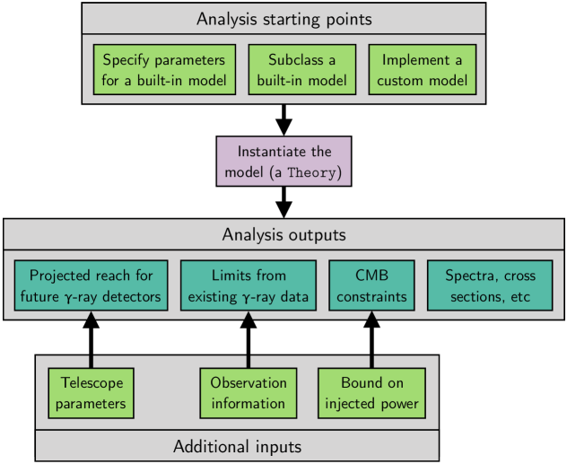
Figure 1: Overview of the workflow, showing different starting points for analyzing sub-GeV dark matter models and possible outputs. The light green boxes at the top show different types of models the user can analyze. After a model has been instantiated (purple box), various functions can be called to compute the outputs in the dark green boxes. The inputs in the lower light green boxes are required to compute the three corresponding indirect detection constraints.

In this section, we describe the structure of the hazma is shown in Fig. (2). The light green boxes at the top indicate the types of physics models a user can study, the dark green boxes show possible analysis outputs, and the light green boxes at the bottom denoting inputs required for these outputs. The user has several options for tapping into the resources provided by sec:models_scalar_mediator

) and Sec. (LABEL:sec:models_vector_mediator) for details on the built-in models and their corresponding parameters). Alternatively, if the user is working with a model which is a specific version one of the included models (e.g., where the mediator’s couplings to Standard Model particles are interrelated), they can define their own subclass of that model. By using inheritance, one retains all of the functionality of the built-in model (such as functions for computing final state radiation spectra, cross sections, mediator decay widths, etc.) while supplying the user with a simpler, more specialized interface to the underlying models. For a detailed explanations of how to set model parameters and make subclasses of built-in models, see App. (LABEL:sec:basic_usage). Another option is for the user to define their own model. To do this, they need to define a class which contains functions for the gamma-ray and positron spectra, as well as the annihilation cross sections and branching fractions. In App. (LABEL:sec:usage) we provide a detailed example of how to do this for a toy model, utilizing various helper modules provided by After choosing a model, the user represents it in Theory class (purple box in Fig. (2)). Various particle physics quantities (the DM self-annihilation cross section, gamma-ray spectra per DM annihilation, etc) can be computed using the values of the masses and couplings in the fig:user_workflow). To make it straightforward for the user to constrain models using existing data, figure[tbh!] Structure of . At the core of are modules for computing gamma-ray and positron spectra: , and missing. The module contains the class, which possesses methods for computing limits on models MeV gamma-ray telescopes. comes with predefined models located in the and modules. These have pre-implemented functions for computing the decay, FSR, and positron spectra, mediator branching fractions, and DM self-annihilation cross sections. Fig. (2) displays the modules contained in missing The primary goal of Theory abstract base class, which every dark matter model in Theory.binned_limit), one for computing the discovery reach for planned gamma-ray detectors (Theory.cmb_limit). The class also provides methods for computing particle physics quantities such as annihilation cross sections (with partial_widths), the continuum and monochromatic gamma-ray spectra from DM annihilation (gamma_ray_lines), and the same for positron spectra (positron_lines), and more. Custom models must implement functions for computing gamma-ray spectra, positron spectra and branching fractions to gain use of the methods in As mentioned above, Appendix (LABEL:sec:usage) shows how to implement a simple custom model. Two other modules may be useful for complex custom models: missing This contains high-performance functions for computing the decay spectra from $\pi^{\pm},\pi^{0}$ and $\mu^{\pm}$. Details of how these are computed are found in Sec. (LABEL:sub:radiative_decay_spectra). The functions in this module allow the user to compute the decay spectra for particles decaying with arbitrary lab-frame energies. This requires computing the decay spectra in the rest frame of the parent-particle and performing a Lorentz boost, amounting to performing a change-of-variables along with a convolution integral. To achieve high computational performance, we perform all integrations in cython [behnel2011cython] and build extension modules to interface with python.

missing

This module computes the electron/positron spectra from decays of $\pi^{\pm}$ and $\mu^{\pm}$, which are critical inputs for constraining dark matter models using CMB observations. See Sec. (LABEL:sec:dm_positron_spectra) for details on how these spectra are computed. As in the positron_spectra module allows users to compute the electron/positron spectra for arbitrary energies of the parent-particle. The procedure for computing the spectra for arbitrary parent-particle energies is identical to the procedure used for hazma also ships with various particle physics models of sub-GeV DM. These models are located in the modules vector_mediator, and contain all the relevant annihilation cross sections, branching fractions, decay spectra, FSR spectra and positron spectra. They can be used by instantiating the appropriate class (for example, the scalar_mediator for the Higgs-portal model.) The user only needs to specify the parameters of the model. The particle physics frameworks used to construct these models, the specialized subclasses of these models included with , and accessing functions to compute their annihilation cross sections and other particle physics quantities is the topic of the following section.

3 Particle physics framework

Each of the models distributed with align L& = L_SM + L_DM + L_M + L_Int(M), which consists of the SM Lagrangian, the free Lagrangians for the Dark Matter (DM) and mediator (M), and the mediator’s interactions with the DM and SM fields, collectively included in the term $\mathcal{L}_{{\mathrm{Int}}(M)}$. For the models currently available in align L_DM = ¯χ (i ／∂- m_χ) χ. Both the dark matter and the mediator are taken to be uncharged under the Standard Model gauge group. The Lagrangian is defined in terms of the microscopic degrees of freedom of the Standard Model (quarks, leptons and gauge bosons). However, at the energy scale of interest for self-annihilations of non-relativistic MeV dark matter ($\sqrt{s}\sim 1-100~{}\mathrm{MeV}$), quarks and gluons are not the correct strongly-interacting degrees of freedom. At these energies, QCD confines, and quarks and gluons group into bound states called mesons and baryons. Given that the DM interacts with quarks and gluons, at these energies interactions with mesons and baryons are induced. Since QCD is non-perturbative for energies $\sqrt{s}\lesssim\mathrm{GeV}$, we must use an effective field theory to describe the interactions of DM with mesons and baryons. We thus match our microscopic Lagrangian onto the effective Lagrangian for pions and other mesons using the techniques of chiral perturbation theory (ChPT) [WEINBERG1979327, Gasser:1983yg, GASSER1985465, ecker1995chiral, Scherer2003]. The models currently implemented in ChPT ∼4 πf_π≈1.2 GeV$,where$f_π= 92.2 MeV$isthepiondecayconstant.Derivativesofthemesonfieldsandfactorsofthemesonmassesarecountedas$O(p)$.Theexpansionparameter$p^2$isusedintwoways.First,thechiralLagrangianisorganizedasasumoftermsofdecreasingimportance\begin{aligned} \mathcal{L}_{\mathrm{ChPT}}=\mathcal{L}^{(2)}+\mathcal{L}^{(4)}+\mathcal{L}^{(6)}+\dots,\end{aligned}wherethesuperscriptindicatesthenumberofderivativesorpowersofmesonmasses.Second,theexpansionparametercanbeusedtoassesstherelativesizeofanindividualFeynmandiagram^{\prime}scontributioninthecalculationofagivenobservable.Thisisquantifiedusingthe\emph{chiral dimension},whichislowerformoreimportantdiagrams.Generallythetree-leveldiagramsfrom$L^(2)$havethelowestchiraldimensionandprovidethelargestcontributionstoobservables,followedbytree-leveldiagramsfrom$L^(4)$andone-loopdiagramsfrom$L^(2)$,andsoon.As$p^2 →Λ_ChPT^2$,thisschemefororganizingcalculationsintermsofthechiraldimensionbreaksdownandChPTbecomesunreliable.\par Assessingthepreciserangeofvalidityofleading-orderChPTiscomplicated.Asimpleestimatesuggeststhatforprocesseswithmesonenergiesofe.g.$500 MeV$theleading-orderobservablesreceive$∼(500 MeV / Λ_ChPT)^2 ∼20%$correctionsfromnext-to-leading-order(NLO)contributions~{}\cite[cite]{[\@@bibref{Number}{Pich:1995bw}{}{}]}.Inreality,themagnitudeofNLOcorrectionsislargerforannihilationfinalstateswiththesamequantumnumbersasresonancessuchasthe$ρ$~{}\cite[cite]{[\@@bibref{Number}{Meissner:1993ah}{}{}]}and$f_0(500)$~{}\cite[cite]{[\@@bibref{Number}{f0500_review}{}{}]},sincethefinalstateparticlescanrescatter.Whileresonancescanbeaccountedforwithunitarizationtechniques~{}\cite[cite]{[\@@bibref{Number}{PhysRevLett.61.2526,f0500_review}{}{}]}orasexplicitresonancefields~{}\cite[cite]{[\@@bibref{Number}{ECKER1989311,Soto:2011ap}{}{}]},weinsteaduseleading-orderChPT,restrictingtoDMmassesbelow250MeVinthecaseofannihilationintoStandard-Modelparticlesandmediatormassesbelow500MeVforanalysisoftheirdecaystoavoidresonances.AnimportantconsequenceisthatannihilationintokaonsandheaviermesonsisnotconsideredhereinsincethatwouldrequireDMmassesfarabovethisrange.User-definedmodels(seeApp.~{}(\ref{app:user_defined_models}))neednotuseleading-orderChPT,andthisisaninterestingtopicforfuturework.\par Whiletheprecedingdiscussionisquitegeneral,wenowspecializetothetwomodelsthatcomewith\verb{}{hazma}: \mil{}{hazma}: \milscalar_{m}ediator,whichcontainsarealscalarmediator$S$,and\verb{}{vector_mediator}, where the mediator is a vector $V$~\footnote{}{vector_mediator}, where the mediator is a vector $V$~\footnoteInfuturework,weplantoaddpseudoscalarandaxial-vectormediators..Thesearesubclassesoftheabstractclass\verb{}{Theory}, and thus implement a variety of functions for computing physical quantities. In the following two subsections, we present $\L_{}{Theory}, and thus implement a variety of functions for computing physical quantities. In the following two subsections, we present $\L_{\mathrm{Int}}(S)$ and $\mathcal{L}_{{\mathrm{Int}}(V)}$ at the level of quarks and gluons as well as the Lagrangians obtained by performing the ChPT matching. Snippets are provided to demonstrate how to construct each model and change its parameters. The third subsection shows how to access various particle physics quantities in Scalar Mediator The free Lagrangian for a real scalar is

$$\mathcal{L}_{S} =\frac{1}{2}(\partial_{\mu}S)(\partial^{\mu}S)-\frac{1}{2}m_{S}^{2}S^{2},$$ (3.1)

where $m_{S}$ is the scalar’s mass. The interactions with the light fundamental SM degrees of freedom read

$$\mathcal{L}_{{\mathrm{Int}}(S)} =-S\left(g_{S\chi}+g_{Sf}\sum_{f}\frac{y_{f}}{\sqrt{2}}\bar{f}f\right)$$ (3.2)

$$\hskip 56.9055pt+\frac{S}{\Lambda}\left(g_{SG}\frac{\alpha_{\mathrm{EM}}}{4\pi}F_{\mu\nu}F^{\mu\nu}+g_{SF}\frac{\alpha_{s}}{4\pi}G_{\mu\nu}^{a}G^{a\mu\nu}\right).$$

The sum runs over fermions with mass below the GeV scale ($f=e,\mu,u,d,s$). Note that the coupling $g_{Sf}$ is outside the sum. The Yukawa couplings are defined to be $y_{f}=\sqrt{2}m_{f}/v_{h}$, with the Higgs vacuum expectation value (vev) defined as $v_{h}=246{~{}\mathrm{GeV}}$. The parameter $\Lambda$ is the mass scale at which $S$ acquires (non-renormalizable) interactions with the photon and gluon. After performing the matching onto the chiral Lagrangian and expanding to leading order in the pion fields, the resulting interaction Lagrangian is

$$\mathcal{L}_{\mathrm{Int}(S)} =\frac{2g_{SG}}{9\Lambda}S\left[(\partial_{\mu}\pi^{0})(\partial^{\mu}\pi^{0})+2(\partial_{\mu}\pi^{+})(\partial^{\mu}\pi^{-})\right]$$ (3.3)

$$\hskip 28.45274pt+\frac{4ieg_{SG}}{9\Lambda}SA^{\mu}\left[\pi^{-}(\partial_{\mu}\pi^{+})-\pi^{+}(\partial_{\mu}\pi^{-})\right]$$

$$\hskip 28.45274pt-\frac{B(m_{u}+m_{d})}{6}\left(\frac{3g_{Sf}}{v_{h}}+\frac{2g_{SG}}{3\Lambda}\right)S\left[(\pi^{0})^{2}+2\pi^{+}\pi^{-}\right]$$

$$\hskip 28.45274pt+\frac{B(m_{u}+m_{d})g_{SG}}{81\Lambda}\left(\frac{2g_{SG}}{\Lambda}-\frac{9g_{Sf}}{v_{h}}\right)S^{2}\left[(\pi^{0})^{2}+2\pi^{+}\pi^{-}\right]$$

$$\hskip 28.45274pt+\frac{4e^{2}g_{SF}}{9\Lambda}S\pi^{+}\pi^{-}A_{\mu}A^{\mu}$$

$$\hskip 28.45274pt-g_{S\chi}S\bar{\chi}\chi-g_{Sf}S\sum_{\ell=e,\mu}\frac{y_{\ell}}{\sqrt{2}}\bar{\ell}\ell.$$

where $B=m_{\pi^{\pm}}^{2}/(m_{u}+m_{d})\approx 2800$ MeV [ecker1995chiral]. The parameters for the scalar model are attributes of the hazma are

$$(m_{\chi},m_{S},g_{S\chi},g_{Sf},g_{SG},g_{SF},\Lambda)\leftrightarrow(\mathtt{mx},\mathtt{ms},\mathtt{gsxx},\mathtt{gsff},\mathtt{gsGG},\mathtt{gsFF},\mathtt{lam}).$$

The following snippet shows how to instantiate mintedpython >>> from hazma.scalar_mediator import ScalarMediator >>> sm = ScalarMediator(mx=150., ms=1e3, gsxx=1., gsff=0.1, … gsGG=0.1, gsFF=0.1, lam=2e5) >>> sm.gsff 0.1 >>> sm.gsff = 0.5 >>> sm.gsff 0.5 In addition to the general hazma also comes with two subclasses of Krnjaic:2015mbs (HeavyQuark.) The Higgs-portal model assumes the scalar mediator interacts with the Higgs through gauge-invariant interactions resulting in the scalar mediator mixing with the Higgs. After diagonalizing the scalar-mediator/Higgs mass matrix, the scalar mediator and Higgs are replaced with:

$$h \to h\cos\theta-S\sin\theta, S \to h\sin\theta+S\cos\theta$$ (3.4)

where $\theta$ is the scalar-mediator/Higgs mixing angle. This replacement results in the following cutoff scale and couplings of the scalar mediator with the Standard Model fermions, gluons and photon, the later of which require integrating out the $\tau$, $c$, $b$, $t$, $W$ and $Z$ [Marciano:2011gm]:

$$g_{Sf} =\sin\theta, g_{SG} =3\sin\theta, g_{SF} =-\frac{5}{6}\sin\theta, \Lambda =v_{h}.$$ (3.5)

where $v_{h}=246\ \mathrm{GeV}$ is the Higgs vacuum expectation value. The parameters for the align (m_χ, m_S, g_Sχ, sinθ) ↔(mx, ms, gsxx, stheta). The heavy-quark model assumes the existence a new heavy, colored and charged fermion which enters the Lagrangian as:

$$\mathcal{L}\supset i\bar{Q}\not{D}Q-m_{Q}\bar{Q}Q-\frac{m_{Q}}{v_{h}}h\bar{Q}Q-g_{SQ}S\bar{Q}Q$$ (3.6)

with $D_{\mu}=\partial_{\mu}-ieQ_{Q}A_{\mu}-ig_{s}G_{\mu}^{a}\lambda^{a}/2$ where $Q_{Q}$ is the $\operatorname{U}_{\mathrm{EM}}(1)$ charge of the heavy-quark. Integrating out the heavy quark induces a cutoff scale and effective couplings of the scalar mediator with gluons and photons:

$$g_{SG} =g_{SQ}, g_{SF} =2Q_{Q}^{2}g_{SQ}, \Lambda =m_{Q}.$$ (3.7)

Note that integrating out the heavy-quark also induced effective couplings to the SM fermions, but at two-loop order. We do not include these interactions. The parameters for the align (m_χ, m_S, g_Sχ, g_SQ, m_Q, Q_Q) ↔(mx, ms, gsxx, gsQ, mQ, QQ). Both of these models can be imported and used in a similar fashion to the generic mintedpython >>> from hazma.scalar_mediator import HiggsPortal, HeavyQuark >>> hp = HiggsPortal(mx=150., ms=1e3, gsxx=1., stheta=1e-3) >>> hq = HeavyQuark(mx=150., ms=1e3, gsxx=1., gsQ=1.0, mQ=1e6, QQ=1.) Trying to set the underlying mintedpython >>> hp.gsff # can only be accessed 0.001 >>> hp.gsff = 0.1