Time-Series Machine Learning Error Models for Dynamical Systems

1 Introduction

Engineering design and scientific analysis often requires many queries of a computational model. Examples of such many-query processes include uncertainty quantification, design optimization, and statistical inference. For these many-query problems, the cost of the forward evaluation of the computational model is often a bottleneck and, in some cases, prohibitively expensive. As such, it is common for analysts to rely on low-cost models that generate approximate solutions to a high-fidelity “truth” model. While many low-cost models are discipline-specific, general examples include linearized models, coarse-mesh discretizations of partial differential equations, and projection-based reduced-order models. The use of such low-cost models alleviates the computational burden of the high-fidelity forward model evaluation and makes the many-query problem computationally tractable.

As low-cost models generate approximate solutions, it is critical to quantify the error in the approximation. Quantifying errors in approximate models has recieved significant attention in a variety of communities. Within the reduced-order modeling community, research has examined the development of both rigorous and approximate a posteriori error bounds for linear and non-linear problems, as well as approximate error models. In [reduced_basis_output_apost], rigorous a posteriori error bounds for quantity-of-interest errors (QoI) for the reduced-basis method applied to linear elliptic partial differential equations were developed. Extensions to linear time-dependent parabolic PDEs were considered in [grepl_patera_apost, rovas_apost]. Similarly, a posteriori bounds on state errors for POD reduced-order models are constructed in Refs. . In the context of non-linear model reduction of dynamical systems, rigorous a posteriori error bounds for the Galerkin and least-squares Petrov-Galerkin reduced-order models were derived in Ref. [carlberg_lspg_v_galerkin]. Linearized error bounds for the Galerkin method were derived in [homescu_romlinbounds]. The aformentioned references are all analagous in that the error bounds are derived from analysis of the full-order and reduced-order models. The error bounds derived from these methods are residual-based, meaning that they depend on the (dual) residual of the full-order problem of interest.

When deployed on non-linear dynamical systems of interest, both approximate and rigorous error bounds suffer on several fronts. The most challenging issue is that, for non-linear dynamical systems, rigorous error bounds grow exponentially in time and are often not tight. This limits the praticality of such methods. Another challenge is that both approximate and rigorous error bounds typically require the evaluation of the full-order residual and/or the solution to the dual (adjoint) problem, both of which scale with the number of degrees of freedom of the full-order model. Further, the software required for formulating and solving the dual problem required for adjoint-based methods is often unavailable and challenging to implement.

With the growing availability in data and interest in machine learning, recent research has examined the construction of machine learning error models. In contrast to error bounds, error models seek to directly approximate state and QoI errors through regression techniques. In Ref. [carlberg_ROMES], Carlberg and co-workers developed the ROMES method. The ROMES method uses Gaussian Process regression to map error indicators (such as residual norms) to both state and QoI errors in reduced-order models. More recently, the ROMES method has been examined as a tool for constructing in-plane and out-of-plane error models for each generalized coordinate in steady-state reduced-order models [romes_closure]. The ROMES method has been shown to be capable of providing accurate state-error and quantity of interest predictions as well as a notion of probabalistic rigor.

Two significant drawbacks of the ROMES method are that 1.) the method is based on Gaussian Process regression, which suffers from the curse of dimensionality, and 2.) the extension of the ROMES method to dynamical systems is unclear. To address these issues, two follow-up works have been pursued. In Ref [freno_carlberg_ml], this first issue was addressed through the construction of statistical error models via high-dimensional machine learning techniques. The approach is similar in spirit to the ROMES method, but uses modern machine learning techniques (such as artificial neural networks) with more sophisticated input features than originally considered in ROMES. This approach circumvents the dimensionality problem from which the ROMES method suffers. The approach was shown to be capable of providing highly accurate predictions of both the normed state error and QoI error. The extension of the approach to dynamical systems was not considered. In Ref [trehan_ml_error], the extension of the ROMES method to reduced-order models of dynamical systems was examined. Similar to Ref. [freno_carlberg_ml], Ref. [trehan_ml_error] (which came before Ref. [freno_carlberg_ml]) used high-dimensional machine larning algorithms to map a (potentially large) set of input features to state and QoI errors in dynamical systems. This framework was referred to as the error modeling via machine learning (EMML) framework. In addition to acting as a stand-alone error model, the EMML framework examined using the output of the machine learning model as an input feature for the ROMES method, thus merging the two approaches. In Ref. [trehan_ml_error], the EMML framework was shown to be capable of providing accurate predictions for quantity-of-interest errors in a multiphase subsurface flow problem. A limitation of the EMML framework, however, is that it approaches the machine learning problem for dynamical systems as a stationary regression problem opposed to as a time-series problem. As errors in dynamical systems are non-local in time, the EMML framework does not necessarily have a physically-consistent setting. Problem-specific considerations, such as the time-domain decompositions and non-Markovian input features used in Ref. [trehan_ml_error], may be required for accurate results.

The objective of this work is to extend the error modeling framework developed by Freno and Carlberg in Ref. [freno_carlberg_ml] to approximate solutions of dynamical systems. To properly address the non-Markovian effects inherent to dynamical system errors, the present work considers high-dimensional regression methods from deep learning that are capable capturing memory effects. These methods include recurrent neural networks [rnn_rumelhart] and the long short-term memory networks [lstm_hochreiter]. Standard Markovian regression methods, as considered in the EMML framework, are also considered. The format of the manuscript is as follows: Section 2 outlines parameterized dynamical systems, approximate solutions, and traditional error quantification methods. Section 3 outlines the machine learning framework used in this work. Feature engineering, data generation, machine learning training, and stochastic noise modeling are discussed. Section 4 applies the proposed framework to 1.) a POD reduced-order model of the advection-diffusion equation, 2.) a POD reduced-order model of the shallow water equations, and 3.) a coarse numerical simulaiton of the Burgers’ equation. Conclusions are provided in Section 5.

2 Parametrized Dynamical Systems

This work considers the parameterized dynamical system,

$$\frac{d}{dt}\boldsymbol{x}=\boldsymbol{f}(\boldsymbol{x},\boldsymbol{\mu}),\qquad\boldsymbol{x}(0)=\boldsymbol{x}_{0},\qquad t\in[0,T],$$ (1)

where $T\in\mathbb{R}^{+}$ is the final time, $\boldsymbol{x}\in\mathbb{R}^{N}\times[0,T]$ is the state, $\boldsymbol{x}_{0}\in\mathbb{R}^{N}$ the initial conditions, $\boldsymbol{\mu}\in\mathbb{R}^{\boldsymbol{\mu}}$ the parameters, and $\boldsymbol{f}:\mathbb{R}^{N}\times\mathbb{R}^{N_{\mu}}\rightarrow\mathbb{R}^{N}$ the velocity. Equation 1 can arise in a variety of contexts, including the numerical discretization of a partial differential equation.

Obtaining numerical solutions to Eq. 1 typically requires some type of temporal discretization (i.e. Runge Kutta schemes, space-time schemes, etc.). This temporal discretization is obtained by partitioning the time domain into $N^{t}$ equally spaced time-windows of width $\Delta t$. Temporal discretization then results in a sequence of (non-linear) algebraic equations,

$$\boldsymbol{r}^{i}(\mathbf{u}^{i},\mathbf{u}^{i-1},\ldots,\mathbf{u}^{i-M},\boldsymbol{\mu})=\mathbf{0},\qquad\text{for }i\in\mathcal{N}_{FOM}$$ (2)

where the superscripts $i$ refer to $i_{th}$ time-step, $M$ is the width of the time-discretization stencil, and $\mathcal{N}_{FOM}=\{1,2,\ldots,N^{t}\}$, with $N^{t}$ being the number of time-steps. Solving Eq. 2 results in a sequence of $N^{t}$ solutions,

$$\mathbf{U}=\begin{bmatrix}\mathbf{u}^{1}&\mathbf{u}^{2}&\ldots&\mathbf{u}^{N^{t}}\end{bmatrix}.$$

In many scenarios, the response of Eq. 1 is sought for many parameter instances over long time-windows. It is often the case, however, that directly solving Eq. 1 is computationally expensive. In this case, directly obtaining solutions to Eq. 1 for many parameter instances and/or long time-windows is not practical. In such scenarios, low-cost models that generate approximate solutions to Eq. 1 are used.

2.1 Approximate Solutions

Due to the computational expensive of solving high-fidelity full-order model, it is common to use an alternative low-cost model that generates approximate solutions to the full-order model. In this work, it is assumed that there exists an approximate dynamical system,

$$\frac{d}{dt}\hat{\boldsymbol{x}}=\boldsymbol{f}_{R}(\hat{\boldsymbol{x}},\boldsymbol{\mu}),\qquad\hat{\boldsymbol{x}}(0)={\hat{\boldsymbol{x}}}_{0},\qquad t\in[0,T],$$ (3)

where $\hat{\boldsymbol{x}}\in\mathbb{R}^{K}\times[0,T]$ denotes an approximate solution, $\boldsymbol{a}_{0}\in\mathbb{R}^{K}$ the initial conditions, and $\boldsymbol{f}_{R}:\mathbb{R}^{K}\times\mathbb{R}^{N_{\boldsymbol{\mu}}}\rightarrow\mathbb{R}^{K}$ the reduced-velocity. It is further assumed that their exists a prolongation operator that allows the approximate solution to be expressed in the state-space associated with the full system,

$$\boldsymbol{x}\approx\hat{\boldsymbol{x}}=\mathbf{p}(\hat{\boldsymbol{x}}),$$

where $\mathbf{p}:\mathbb{R}^{K}\rightarrow\mathbb{R}^{N}$ is the prolongation operator.

Similar to the full-order model, obtaining solutions to Eq. 3 typically requires some type of temporal discretization. The time-discretiaiton of the approximate model is obtained by partitioning the time-domain into $N^{t}_{r}$ equally spaced time intervals of width $\Delta t_{R}$. Here, we assume that the approximate model is discretized on a subset of the full-order model grid, $\Delta t_{R}=R_{r}\Delta t$, with $R_{r}\in\mathbb{Z}^{+}$ being a positive integer. This leads to a sequence of algebraic equations,

$$\boldsymbol{r}_{R}^{i}(\hat{\boldsymbol{x}}^{i},\hat{\boldsymbol{x}}^{i-1},\ldots,\hat{\boldsymbol{x}}^{i-M},\boldsymbol{\mu})=\mathbf{0},\qquad\text{for }i=\mathcal{N}_{ROM}$$ (4)

where the superscripts $i$ refer to $i_{th}$ time-step of the approximate model, $M_{r}$ is the width of the time-discretization stencil of the approximate model, and $\mathcal{N}_{ROM}=\{1,2,\ldots,N^{t}_{r}\}$ with $N^{t}_{r}$ being the number of time-steps in the approximate model. It is noted that $N^{t}_{r}$ is typically smaller than $N^{t}$ as approximate models are often capable of taking larger time-steps than full-order models [1]. Solving Eq. 4 results in a sequence of $N^{t}_{r}$ solutions,

$$\mathbf{A}_{r}=\begin{bmatrix}\hat{\boldsymbol{x}}^{1}&\hat{\boldsymbol{x}}^{2}&\ldots&\hat{\boldsymbol{x}}^{3}\end{bmatrix}.$$

Various types of approximate models exist. This work considers applications to low-fidelity models and proper orthogonal decomposition (POD) reduced-order models.

2.1.1 Low-Fidelity Models

Low-fidelity models are a type of approximate model that generate approximate solutions to the full-order model by solving a system that is of lower fidelity than the original high-order mdoel. Types of low-fidelity models incldue coarse-grid numerical simulations, linearized systems, and systems with reduced physics.

2.1.2 POD Reduced-Order Models

Projection-based reduced-order models are a popular technique for generating computationally efficient approximations to full-order models. Projection-based ROMs operate by approximating the full-dimensional state vector on a $K$-dimensional affine trial space,

$$\boldsymbol{x}\approx\hat{\boldsymbol{x}}=\basisvec\hat{\boldsymbol{x}}+\boldsymbol{x}_{0},$$ (5)

where $\boldsymbol{\Phi}\in\mathbb{R}^{N\times K}$ is the trial basis matrix with orthogonal column vectors and $\boldsymbol{a}\in\mathbb{R}^{K}$ the generalized coordinates. Typically, $\boldsymbol{\Phi}$ is obtained through a dimension reduction process such as proper orthogonal decomposition. A dynamical system can be obtained for the generalized coordinates through projection of the original high-fidelity model,

$$\boldsymbol{\Psi}^{T}\bigg{[}\frac{d}{dt}\hat{\boldsymbol{x}}-\boldsymbol{f}(\hat{\boldsymbol{x}},\mu)\bigg{]},\qquad\hat{\boldsymbol{x}}(0)={\hat{\boldsymbol{x}}}_{0},$$ (6)

Possible projections include Galerkin, least-squares Petrov Galerkin, and adjoint Petrov-Galerkin projection, given respectively as,

$$\boldsymbol{\Psi}_{G} =\boldsymbol{\Phi},$$ (7)

$$\boldsymbol{\Psi}_{LSPG} =\boldsymbol{\Phi}\bigg{[}\mathbf{I}-\alpha\Delta t\frac{\partial\boldsymbol{f}}{\partial\boldsymbol{x}}^{T}\bigg{]},$$ (8)

$$\boldsymbol{\Psi}_{APG} =\boldsymbol{\Phi}\bigg{[}\mathbf{I}+\tau\frac{\partial\boldsymbol{f}}{\partial\boldsymbol{x}}\bigg{(}\mathbf{I}-\boldsymbol{\Phi}\boldsymbol{\Phi}^{T}\bigg{)}\bigg{]}.$$ (9)

This work focuses on the Galerkin projection but applies to other projections.

2.2 Reduced-order Model Error

Reduced-order methods seek approximations ($\hat{\boldsymbol{x}}$) to the full-order model ($\boldsymbol{x}$). Quantifying the error incurred by this approximation is thus important. This work focuses on quantifying two types of error:

1. The normed state-error: $\left\lVert\boldsymbol{e}(\boldsymbol{\mu},t)\right\rVert_{2}:=\left\lVert\boldsymbol{x}(\boldsymbol{\mu},t)-\hat{\boldsymbol{x}}(\boldsymbol{\mu},t)\right\rVert_{2}.$

2. Quantity of interest error: $\delta_{q}=g(\boldsymbol{x}(\boldsymbol{\mu},t))-g(\hat{\boldsymbol{x}}(\boldsymbol{\mu},t)),$

where $g:\mathbb{R}^{N}\rightarrow\mathbb{R}$ is the state-to-QoI map.

2.3 The Residual as an Error Indicators

Commonly employed techniques for quantifying the normed state and quantity of interest errors are typically based on rigorous a posteriori error bounds (normed state error) and dual weighted residuals (QoI error). A significant body of work examining error estimation and error bounds exists in discipline specific literature. To name a few, error bounds are derived in the context of projection-based reduced order models in Refs. [carlberg_lspg_v_galerkin, rovas_apost, homescu_romlinbounds, grepl_patera_apost]. Error models for quantity of interest and discretizatin errors in the context of under-resolved numerical simulalations are considered in Refs. [ackmann_errorestimation, lu_phd_thesis]. Error bounds and quantity of interest errors in the context of approximate solutions to steady systems were presented in Ref. [freno_carlberg_ml].

While the exact setting of these different error models and error bounds varies, an important observation is that they are all methods are tied to the residual of the system of interest. The residual appears as a driving factor in both quantity of interest and solution normed error indicators and models. As such, the residual is viewed as a critical featuer required for error estimation.

3 Machine Learning Error Models

The aim of this work is to construct machine learning regression models for errors of interest. This work uses the framework developed by Freno and Carlberg in [freno_carlberg_ml] to construct these regression methods. The distinction between the current work and that presented in [freno_carlberg_ml] is that, here, errors are non-local in time. Due to this, a different set of learning algorithms and considerations are required. Similar to Ref. [freno_carlberg_ml], this work considers high-dimensional learning techniques that allow for a variety of input features.

3.1 Machine Learning Framework

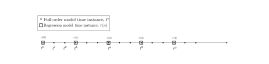
This work develops machine learning models aimed at predicting errors of interest on a subset of the approximate model temporal grid. This grid is defined by partitioning the the time interval $[0,T]$ into $N_{ML}$ windows of length $\Delta t_{ML}=R_{ML}\Delta t_{R}$, where $R_{ML}\in\mathbb{Z}^{+}$ is an integer greater than or equal to one. The size of these time-windows are equal to or larger than that of the approximate model. A reference is provided in Figure 1, where $R_{ML}=2$ and $R_{R}=3.$

Figure 1: Example of time discretizations for the full-order model, approximate model, and machine learning model. In this case, the approximate model is solved on a temporal grid 3 times coarser than the full-order model. The regression model is solved on a temporal grid that is twice as coarse as the approximate model.

Let $\boldsymbol{\rho}^{i}(\boldsymbol{\mu},\hat{\boldsymbol{x}}^{i},t^{i})\in\mathbb{R}^{N_{\rho}}$ denote a vector of $N_{\rho}$ features at the $i_{th}$ time-step of the machine learning temporal grid,

$$\boldsymbol{\rho}^{i}(\boldsymbol{\mu},\hat{\boldsymbol{x}}^{i},t^{i})=\{\rho_{1}^{i},\rho_{2}^{i},\rho_{3}^{i},\ldots,\rho_{N_{\rho}}^{i}\}.$$

Similarly, let $\featuremat^{i}$ denote the compiled set of all feature vectors up until $t^{i}$,

$$\featuremat^{i}=\{\boldsymbol{\rho}^{1},\boldsymbol{\rho}^{2},\ldots,\boldsymbol{\rho}^{i}\}.$$

Given this set of features, this work models the feature-to-error mapping $\featuremat^{i}\rightarrow\delta^{i}$ to be the combination of a deterministic function and an additive mean-zero noise model,

$$\delta^{i}(\featuremat^{i})\approx{f}(\featuremat^{i})+\epsilon(\featuremat^{i}),\qquad\text{for }i=1,2,...,N_{ML}.$$ (10)

In the above, ${f}$ refers to the deterministic function and $\epsilon$ is the mean-zero noise model. The noise model is responsible for accounting for the statistical uncerainty that arrises due to the lack of explanatory features.

The framework used here constructs regression models for both the deterministic component of the mapping (${f}$) and the noise noise,

$$\hat{\delta}^{i}(\featuremat^{i})\approx{\hat{f}}(\featuremat^{i})+\hat{\epsilon}(\featuremat^{i}),\qquad\text{for }i=1,2,...,N_{ML}.$$ (11)

The framework proposed in Ref. [freno_carlberg_ml] that is used here to construct approximation given in Eq. 11 consists of four steps:

1. Feature Engineering: The first step is to develop the features, $\boldsymbol{\rho}$, that will be used as inputs into the regression function.

2. Generation of Training Data: After selecting the input features for the regression algorithm, the next step consists of generating of the training data set, $\mathcal{T}_{train}$. The training dataset is constructed through sampling the parameter domain and solving the full-order model and approximate model.

3. Construction and Training of Regression Model: After constructing the training set, a regression function that provides the mapping from $\featuremat^{i}\rightarrow\delta^{i}$ is constructed. This work examines the use of high-dimensional Markovian and non-Markovian machine learning algorithms to obtain the mapping.

4. Construction of the Stochastic Noise Model: The final step involves the construction of a noise model.

3.2 Feature Selection

While, in theory, machine learning algorithms can perform complex tasks such as feature selection, the practically of finite-size datasets and overfitting make machine learning methods sensitive to the input features. This work considers various input feature sets. These feature sets were motivated from Ref. [freno_carlberg_ml].

1. Parameters: This method models the errors as a function of the parameters. The input featuers as the $i_{th}$ time index are,

   $$\boldsymbol{\rho}^{i}=\{\boldsymbol{\mu}\}.$$

   The number of input features in this method is $N_{\rho}=N_{\boldsymbol{\mu}}$. For stationary parameters, this input feature is the same for every time index.

2. Residual Norm: This method uses the instantaneous residual norm as an input feature. This method was used in the original ROMES method [carlberg_ROMES] as well as in Ref. [freno_carlberg_ml]. The input features for this method are,

   $$\boldsymbol{\rho}^{i}=\{\left\lVert\boldsymbol{r}\right\rVert_{2}^{i}\}.$$

   The number of input features in this method is $N_{\rho}=1$.

3. Residual Norm and Parameters: This method uses both the residual norm as well as the parameters as input featuers. In Ref. [2], this was observed to be a more effective than Method 1 for application to steady problems.

   $$\boldsymbol{\rho}=\{\boldsymbol{\mu},\left\lVert\boldsymbol{r}\right\rVert_{2}\}.$$

   The number of input features in this method is $N_{\rho}=N_{\boldsymbol{\mu}}+1$.

4. Residual Norm, Parameters, and Time: The third method considered uses the residual norm, parameters, and time as input features. The inclusion of time as an input feature allows non-recursive regression models to capture non-Markovian effects. It is noted that time was included as an input feature in Ref. [trehan_ml_error]. The input features for this method are given by,

   $$\boldsymbol{\rho}=\{\boldsymbol{\mu},\left\lVert\boldsymbol{r}\right\rVert_{2},t\}.$$

   The number of input features in this method is $N_{\rho}=N_{\boldsymbol{\mu}}+2$.

5. Parameters and Residual: This feature method uses the entire residual vector as well as the parameters,

   $$\boldsymbol{\rho}=\{\boldsymbol{\mu},\boldsymbol{r}\}.$$

   This method is inspired from the fact that both the dual weighted residual and state error norm are driven by the residual. The number of input features in this method is $N_{\rho}=N_{\boldsymbol{\mu}}+N$.

6. Parameters and Residual Principal Components: The residual can be (very) high-dimensional and contain highly correlated features. In the case of limited data, this can prohibit training a generalizable model. The prinicipal components of the residual are considered,

   $$\boldsymbol{\rho}=\{\boldsymbol{\mu},\hat{\boldsymbol{r}},\}$$

   where

   $$\hat{\boldsymbol{r}}=\boldsymbol{\Phi}_{\boldsymbol{r}}^{T}\big{(}\boldsymbol{r}-\overline{\boldsymbol{r}}\big{)}.$$

   The matrix $\boldsymbol{\Phi}_{\boldsymbol{r}}\in\mathbb{R}^{N\times n_{r}}$ comprises of a set of $n_{r}$ orthogonal columns which contain the first $n_{r}$ principal components. The features for this method are then,

   $$\boldsymbol{\rho}=\{\boldsymbol{\mu},\hat{\boldsymbol{r}}\}.$$

   The number of input features in this method is $N_{\rho}=N_{\boldsymbol{\mu}}+n_{r}$.

7. Parameters and Residual Gappy Principal Components: Computing the entire residual, as was required in the previous feature engineering method, is computationally costly due to the fact that it scales with the full-order model. The high-cost associated with computing the residual can be reduced via the gappy POD method [everson_sirovich_gappy]. Gappy POD is a method to reconstruct a signal with missing entries. In this context, the idea behind gappy POD is, instead of sampling the entire residual, to only sample a select few entry points. The residual can then be approximated as,

   $$\hat{\boldsymbol{r}}_{g}=\bigg{(}\mathbf{P}^{T}\boldsymbol{\Phi}_{\boldsymbol{r}}\bigg{)}^{+}\mathbf{P}^{T}\big{(}\boldsymbol{r}-\overline{\boldsymbol{r}}\big{)},$$

   where the superscript $+$ denotes the psuedo-inverse. The matrix $\mathbf{P}\in\mathbb{R}^{N\times N_{s}}$ is a sampling matrix of the form,

   $$\mathbf{P}=\begin{bmatrix}\mathbf{e}_{1}&\mathbf{e_{2}}&\ldots&\mathbf{e}_{N_{s}}\end{bmatrix},$$ (12)

   where $\mathbf{e}_{i}$ is the $i_{th}$ cannonical unit vector and $N_{s}$ the number of sampling points.

   The features for this method are then,

   $$\boldsymbol{\rho}=\{\boldsymbol{\mu},\hat{\boldsymbol{r}}_{g}\}.$$

   The number of input features for this method is the same as the previous feature engineering method, $N_{x}=N_{\mu}+N_{r}$.

8. Sample Residual: The final feature engineering method considers the sampled residual as features,

   $$\boldsymbol{\rho}=\{\boldsymbol{\mu},\mathbf{P}^{T}\boldsymbol{r}\}.$$

   The sampling matrix $\mathbf{P}$ is the same as what was defined in Eq. 12. The total number of input features for this method is $N=N_{\boldsymbol{\mu}}+N_{s}.$

Feature Index	Description	Features	Number of Parameters $N_{\mathbf{X}}$	Number of Residual Elements Required
1	Parameters	$\boldsymbol{\mu}$	$N_{\boldsymbol{\mu}}$	0
2	Residual Norm	$\left\lVert\mathbf{r}\right\rVert_{2}$	$1$	$N$
3	Parameters and residual norm	$[\boldsymbol{\mu},\left\lVert\mathbf{r}\right\rVert_{2}]$	$N_{\boldsymbol{\mu}}+1$	$N$
4	Parameters, residual norm, and time	$[\boldsymbol{\mu},\left\lVert\mathbf{r}\right\rVert_{2},t]$	$N_{\boldsymbol{\mu}}+2$	$N$
6	Parameters and residual	$[\boldsymbol{\mu},\mathbf{r}]$	$N_{\boldsymbol{\mu}}+N$	$N$
7	Parameters and residual principal components	$[\boldsymbol{\mu},\hat{\mathbf{r}}]$	$N_{\boldsymbol{\mu}}+m_{r}$	$N$
8	Parameters and gappy residual principal components	$[\boldsymbol{\mu},\hat{\mathbf{r}}_{g}]$	$N_{\boldsymbol{\mu}}+m_{r}$	$N_{s}$
9	Parameters and sampled residual	$[\boldsymbol{\mu},\mathbf{P}^{T}\mathbf{r}]$	$N_{\boldsymbol{\mu}}+N_{s}$	$N_{s}$

Table 1: Description of feature methods

3.3 Generation of Training Set

After selecting the input features for the regression algorithm, the datasets used to train and test the regression algorithms must be generated. Let $\mathcal{D}$ represent the parameter domain, $\boldsymbol{\mu}\in\mathcal{D}.$ The training dataset is constructed through sampling the parameter domain and solving the full-order model and approximate model. Let,

$$\mathcal{I}_{train}=1,2,\ldots,N_{s},$$

denote the set of sampled parameter instances. Similarly, let

$$\mathcal{J}_{train}=1,2,\ldots,N_{\tau},$$

denote the set of temporal indices included in the training set. With this notation, the training set obtained through solving the full-order and approximate models for samples of the parameter domain can be donted as,

$$\mathcal{T}_{train}=\bigcup_{i\in\mathcal{I}_{train}}\bigcup_{j\in\mathcal{J}_{train}}\mathcal{T}_{i}^{j},$$

with,

$$\mathcal{T}_{i}^{j}=\{\boldsymbol{\rho}^{j}(\boldsymbol{\mu}_{i}),\delta^{j}(\boldsymbol{\mu}_{i})\}.$$

3.3.1 Training Data for Principal Component Analysis and Q-Sampling

Feature engineering methods 6 and 7 require the computation of the prinicipal components of the (gappy) residual vector. These feature methods require additional training data to construct the ressidual basis, $\mathbf{V_{r}}$, and, for gappy POD with Q-sampling, the sampling point matrix. Let,

$$\mathcal{T}_{train,r}=\bigcup_{i\in\mathcal{I}_{train}}\bigcup_{j\in\mathcal{J}_{train}}\mathcal{T}_{i,r}^{j},$$

with,

$$\mathcal{T}_{i,r}^{j}=\{\boldsymbol{r}^{j}(\boldsymbol{\mu}_{i})\}.$$

3.4 Regression Functions

The selection of a regression function that provides the deterministic component of the mapping $\featuremat^{i}\rightarrow\delta^{i}$ is required. This work considers a variety of regression algorithms from supervised machine learning, including neural networks, recurrent neural networks, and long short-term memory networks. This subsection outlines the variety of networks considered.

• K Nearest Neighbors: The simples regression method examined in this work is $K$ Nearest neighbours, in which the prediction is a weighted average of the nearest neighbors in feature space,

  $${\hat{f}}(\boldsymbol{\rho}^{i})=\frac{1}{k}\sum_{i\in\mathcal{I}}\tau(\boldsymbol{\rho},\boldsymbol{\rho})\delta_{i},$$

  where $\mathcal{I}$ denotes the set of $k$ nearest neighbours in feature space.

• Support Vector Regression: Support vector regression (SVR) is used to approximate the regression function as [svr],

  $${\hat{f}}(\boldsymbol{\rho}^{i})=\big{(}\boldsymbol{\theta},\phi(\boldsymbol{\rho}^{i})\big{)}+b,$$

  where $\big{(}\cdot,\cdot\big{)}$ denotes an inner product over the high-dimensional feature space $\mathcal{F}$. SVR aims to find a “flat” function that minimizes the residual while simultaneously seeking a niminal norm of $\big{(}\boldsymbol{\theta},\boldsymbol{\theta}\big{)}$. This is obtained by minimizing the objective function,

  $$\mathcal{J}=\frac{1}{2}\big{(}\boldsymbol{\theta},\boldsymbol{\theta}\big{)}+C.$$

  subject to having all residuals less than $\epsilon$. As it is possible that no such function may satisfy these constraints for all points, SVR employs “slack” variables that allow for deviations away from $epsilon$. The modified optimization problem solved is then,

  $$\mathcal{J}=\frac{1}{2}\big{(}\boldsymbol{\theta},\boldsymbol{\theta}\big{)}+C\sum_{i\in\mathcal{D}_{\text{train}},j\in\mathcal{T}_{\text{train}}}(\zeta^{i}_{j}+\zeta_{i}^{j^{*}}),$$

  $$\delta_{i}^{j}-\big{(}\boldsymbol{\theta},\boldsymbol{\rho})+b\leq\epsilon+\zeta_{i}^{j},\qquad\text{ for }i\in\mathcal{D}_{\text{train}},j\in\mathcal{T}_{\text{train}}$$

  $$\big{(}\boldsymbol{\theta},\boldsymbol{\rho})+b-\delta_{i}^{j}\leq\epsilon+\zeta_{i}^{j^{*}},\text{ for }i\in\mathcal{D}_{\text{train}},j\in\mathcal{T}_{\text{train}}$$

  $$\zeta_{i}^{j^{*}}\geq 0,\qquad\text{ for }i\in\mathcal{D}_{\text{train}},j\in\mathcal{T}_{\text{train}}$$

  $$\zeta_{i}^{j}\geq 0\qquad\text{ for }i\in\mathcal{D}_{\text{train}},j\in\mathcal{T}_{\text{train}}$$

  The term $C$ is the “box constraint” and controls the penalty that is imposed on the size of the error margin. Hyperparameters in SVR are the box constraint C and the theshold $\epsilon$.

• Artificial Neural Networks: Artificial neural networks are commonly employed in machine learning applications. Neural networks rely on function composition to create sophisticated input-to-output maps that, provided sufficient data, can represent complex non-linear functions. In the present context, neural networks are used to build the regression function,

  $${\hat{f}}(\boldsymbol{\rho}^{i},\boldsymbol{\theta})=\mathbf{g}_{N_{layers}}\bigg{(}\cdot,\boldsymbol{\theta}_{N_{layers}}\bigg{)}\circ\mathbf{g}_{N_{layers}-1}\bigg{(}\cdot,\boldsymbol{\theta}_{N_{layers-1}}\bigg{)}\circ\ldots\circ\mathbf{g}_{1}\bigg{(}\boldsymbol{\rho}^{i},\boldsymbol{\theta}_{1}\bigg{)},$$

  where $\mathbf{g}_{i}:\mathbb{R}^{p_{i-1}}\rightarrow\mathbb{R}^{p_{i}}$ denotes the activation function at the $i_{th}$ layer, $i=1,2,\ldots,N_{layers}$ denotes the number of layers, $p_{i}$ denotes the number of neurons at the $i_{th}$ layer for $i>0$, $p_{0}$ is the input feature dimension, and $\mathbf{W}_{i}\in\mathbb{R}^{p_{i-1}\times(p_{i}+1)}$ denotes the weights of the network.

  Figure 2: Diagram for the artificial neural network

  A variety of techniques exist to train neural networks. Here, training is performed through empirical risk minimization with early stopping and regularization. Empirical risk minimization with regularization corresponds to minimizing the mean-squared error over the training set,

  $$\boldsymbol{\theta}=\text{argmin}_{\begin{subarray}{c}\boldsymbol{\theta}\end{subarray}}\sum_{i\in\mathcal{D}_{\text{train}}}\sum_{j\in\mathcal{T}_{\text{train}}}\big{(}{f}(\boldsymbol{\rho}_{i}^{j},\boldsymbol{\theta})-\delta_{i}^{j}\big{)}^{2}+\alpha\left\lVert\boldsymbol{\theta}\right\rVert_{2}^{2},$$

  where $\alpha\in\mathbb{R}^{+}$ is a regularization term. Early-stopping refers to the practice of stopping the minimization algorithm before convergence. The stopping criteria is typically based on monitoring the corresponding loss function on a withheld subset of the training data.

  Hyperparameters in neural networks include can include the number of neurons at each layer, the depth of the ntwork, regularization constants, optimizaton algorithms, early stopping criteria, and activation functions. The number of neurons at each layer, number of layers, and regularization constant are considered as hyperparameters in this work. The Python code to develop the neural networks used in this work with the machine learning package Keras is given in Listing 1.

• Recurrent Neural Networks: Recurrent neural networks are a popular type of neural network for sequence modeling. The main idea of RNNs is to feed the values of the hidden layers of a network at a given point in a sequence into the next point in the sequence. Figure 3 shows the computational graph for an RNN. This work considers recurrent neural networks of various depths and various neurons per layer. The computational rule for an update to a recurrent neural network at the $j_{th}$ timestep is,

  $${\hat{f}}(\boldsymbol{\rho}^{j})=\boldsymbol{z}_{{f}}(\boldsymbol{h}^{j},\boldsymbol{\rho}^{j},\boldsymbol{\theta}),$$

  where $\boldsymbol{h}^{j}$ is a recursive latent state at the $j_{th}$ time-step,

  $$\boldsymbol{h}^{j}=\boldsymbol{z}_{h}(\boldsymbol{\rho}^{j},\boldsymbol{h}^{j-1},\boldsymbol{\theta}),$$

  and $\mathbf{g}_{{f}}$ and $\mathbf{g}_{h}$ are neural networks. Similar to neural networks, the number of neurons at each layer, network depth, and regularization constants are considered as hyper-parameters. The Python code to develop the recurrent neural networks used in this work is given in Listing 2.

  Figure 3: Recurrent neural network with one layer at the $t_{th}$ timestep.

• Long Short-Term Memory (LSTM) Netowrks: LSTM networks are a special type of recurrent networks that are designed to allow for long-term memory dependence. The basis of the LSTM architecture is the cell state. The cell state is a state that runs through the entire sequence and encounters only minor linear interactions. This cell state is capable of capturing long-time dependencies. The Python code to develop the LSTM networks used in this work is given in Listing 3.

  $${\hat{f}}(\boldsymbol{\rho}^{j})=\boldsymbol{z}_{{f}}(\boldsymbol{h}^{j},\boldsymbol{\theta}_{f}),$$

  $$\boldsymbol{h}^{j}=\mathbf{o}^{j}\circ\sigma_{h}(\mathbf{c}^{j})$$

  $$\mathbf{o}^{j}=\sigma_{g}(\boldsymbol{h}^{j},\boldsymbol{\theta}_{o})$$

  $$\mathbf{c}^{j}=\mathbf{l}^{j}\circ\mathbf{c}^{j-1}+\mathbf{i}^{j}\circ\sigma_{c}(\boldsymbol{h}^{j-1},\boldsymbol{\rho}^{j},\boldsymbol{\theta}_{c}),$$

  $$\mathbf{i}^{j}=\sigma_{g}(\boldsymbol{h}^{j-1},\boldsymbol{\rho}^{j},\boldsymbol{\theta}_{i}),$$

  $$\mathbf{l}^{j}=\sigma_{g}(\boldsymbol{h}^{j-1},\boldsymbol{\rho}^{j},\boldsymbol{\theta}_{l})$$

  The variables in the LSTM update rule are:

  • $\boldsymbol{h}^{j}$: hidden state-vector (which is also the output vector) of the LSTM

  • $\mathbf{o}^{j}$: output state vector

  • $\mathbf{c}^{j}$: cell state vector

  • $\mathbf{i}^{j}$: input gate activation vector

  • $\mathbf{l}^{j}$: forget gate activation vector

  Figure 4: Diagram of the Long Short-Term Memory Network

3.5 Training and Model Selection of Machine Learning Algorithms

The regression functions utilizing artificial neural networks, recurrent neural networks, and long short-term memory networks are all implemented in the machine learning package Keras [keras]. These regression functions are trained by minimizing the mean-squared-error of the testing dataset with $L^{2}$ regularization using the Adams algorithm. The Gaussian process regression and nearest neighbour methods are implemented with the Ski-Kit learn package [scikitlearn].

The workflow used for training and testing all machine learning algorithms is as follows:

1. Generate comprehensive dataset, $\mathcal{T}$

2. Extract test and training sets from $\mathcal{T}$: $\mathcal{T}_{train}\cup\mathcal{T}_{test}\subset\mathcal{T}$

3. Normalize all data by the mean and variance of the training set data

4. Perform an $80/20$ split of the training set into a reduced training set and a validation set, $\mathcal{T}_{train}=\mathcal{\overline{T}}_{train}\cup\mathcal{T}_{val}$

5. Train each machine learning model. For the stochastic training algorithms used for the neural networks, LSTMs, and RNNs, train each model $N_{samp}$ times with early stopping. Perform early stopping by withholding $20\%$ of the reduced training set, $\mathcal{\overline{T}}_{train}=\mathcal{\tilde{T}}_{train}\cup\mathcal{\overline{T}}_{earlystopping}$

6. Evaluate the generalization error of the trained model by evaluating the mean squared error on the validation set,

7. Select the model with the best coefficient of determination.

In the limited data case, steps 4 and 5 should be replaced with a cross-validation process.

Noise Model Index	Description	Noise Distribution	Time-dependent
1	Stationary Gaussian Model	Gaussian	No
2	Stationary Laplacian Model	Laplacian	No
3	Autoregressive 1 (AR1)	Gaussian	Yes

Table 2: Description of noise models

3.6 Noise Model

Lastly, a model for the mean-zero noise is required. This work considers a homoscedastic Gaussian and Laplacian models. The following subsections provided a brief description of each method.

3.6.1 Stationary Guassian Homoscedastic Discrepancy Model

The simplest method to quantify the discrepancy between the error model and the true error is to assume the errors to be Gaussian, stationary (no time dependence), and homoscedastic (no feature dependence). The resulting error model is,

$$\epsilon(\mathbf{\eta},t)\approx\mathcal{N}(0,\sigma),$$

where $\sigma$ is the variance of the distribution. These parameters can be obtained through, eg., cross-validation.

3.6.2 Stationary Laplacian Homoscedastic Discrepancy Model

This approach is similar to the first noise model, but this time the errors are assumed to be Laplacian, stationary (no time dependence), and homoscedastic (no feature dependence). The resulting error model is,

$$f(x)\approx\frac{1}{2b}\exp\big{(}-\frac{|x|}{b}\big{)}.$$

where $b$ the diversity.

3.6.3 Autoregressive Gaussian Homoscedastic Discrepancy Model

As errors are expected to display time-correlations, an autoregressive error model is used. The autoregressive error model has the form,

$$\delta^{n+1}=\psi\delta^{n}+\epsilon,$$

where $\psi$ is a constant and $\epsilon$ is mean-zero Gaussian noise.

4 Numerical Experiments

This section explores the performance of the proposed methods.

4.1 Reduced-Order Modeling of the Advection-Diffusion Equation

The first example considers error estimation for reduced-order models of the advection-diffusion equation,

$$\frac{\partial}{\partial t}u(x,t)=p_{0}\frac{\partial u}{\partial x}+p_{1}\frac{\partial^{2}u}{\partial x^{2}},\hskip 7.22743ptu(0,t)=u(2,t)=0,\hskip 7.22743ptu(x,0)=x(2-x)\exp(2x),$$ (13)

on the domain $x\in[0,2]$. The parameter $p_{0}$ controls the wave speed and $p_{1}$ the diffusion. We take $p_{0}$ to be a parameter in the domain of $p_{0}\in[0.1,2]$ and $p_{1}\in[0.1,1]$. The full-order model is taken to be a finite difference scheme that uses central differencing for the diffusion term and upwind differencing for the advection term. The domain, $x$, is partitioned into 101 cells of equal width. After removing the boundary points, the FOM corresponds to the $N=100$ dimensional system of ordinary differential equations,

$$\frac{\partial u_{k}}{\partial t}=p_{0}\frac{u_{k+1}-u_{k}}{\Delta x}+p_{1}\frac{u_{k+1}-2u_{k}+u_{k-1}}{\Delta x^{2}},$$

for $k=1,2,...,N$. The FOM marches the simulation in time using a fourth-order explicit Runge Kutta integrator at a time-step of $\Delta t=0.00015.$

A reduced-order model of the system is constructed by solving the full-order model for a parameter grid of $p_{0}=[0.1,1.05,2.0]$ and $p_{1}=[0.1,0.55,1.0]$. The corresponds to nine total solves of the full-order model. A reduced-basis is constructed by performing POD on the snapshot matrix obtained from stacking the solution snapshots at every $10_{th}$ time-step for $t\in[0,0.3]$. This corresponds to a total of $200$ snapshots. A reduced-order models of dimension $K=5$ is constructed from the POD basis vectors.

4.1.1 Construction of Test and Training Data

This section outlines the construction of the training and testing data for the advection-diffusion numerical example. A large-scale dataset, $\mathcal{T}$, is constructed by solving the full-order and reduced-order models for $1000$ random samples in the parameter domain. The output of the full and reduced-order models is saved every $10_{th}$ time-step, creating $200$ data points for each of the 100 samples. The full dataset is thus given by,

$$\mathcal{T}=\bigcup_{\begin{subarray}{c}i=1\end{subarray}}^{30}\bigcup_{\begin{subarray}{c}j=1\end{subarray}}^{200}\mathcal{T}_{i}^{j},$$

where the subscript $i$ denotes the $i_{th}$ sample, the superscript $j$ denotes the $j_{th}$ saved output of the full-order model, and,

$$\mathcal{T}_{i}^{j}=\{\delta_{i}^{j},\mathbf{x}_{i}^{j}\}.$$

Two training sets generated from $\mathcal{T}$ are considered:

1. Dataset 1: Every fourth saved-output of the first $50$ samples in $\mathcal{T}$ are set to be the training set, while every fourth saved output of the last $50$ samples in $\mathcal{T}$ is the testing set,

   $$\mathcal{T}_{train}=\bigcup_{\begin{subarray}{c}i=1\end{subarray}}^{50}\bigcup_{\begin{subarray}{c}j=1\end{subarray}}^{50}\mathcal{T}_{i}^{4j},\qquad\mathcal{T}_{test}=\bigcup_{\begin{subarray}{c}i=50\end{subarray}}^{100}\bigcup_{\begin{subarray}{c}j=1\end{subarray}}^{100}\mathcal{T}_{i}^{4j}.$$

   To assess the impact of the number of parameter training instances on the regression results, reduced training datasets are constrcuted from $\mathcal{T}_{train}$ by taking,

   $$\mathcal{T}_{train}^{reduced}=\bigcup_{\begin{subarray}{c}i=1\end{subarray}}^{N_{\mathcal{D}train}}\bigcup_{\begin{subarray}{c}j=1\end{subarray}}^{50}\mathcal{T}_{i}^{4j},$$

   with $N_{\mathcal{D}train}\leq 50$.

It is remarked that, for feature methods 5-9, PCA is performed using only the data in the training set. As discussed in section LABEL:sec:error_model, the construction of the stochastic error models is performed using the subset of the training dataset that is withheld for validation.

4.1.2 Regression Results

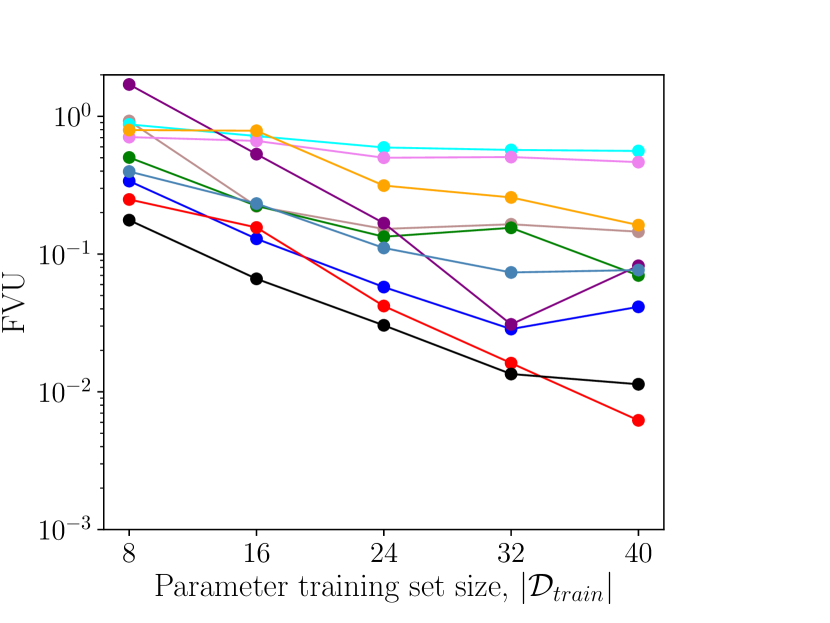
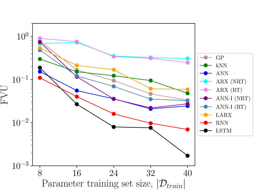
Figure 5 summarizes how the performance of each of the different regression methods varies with the dataset size. Results are shown for the best performing feature method for each regression method. The LSTM network is seen to provide the best predictions for both the normed state error and QoI error, with the exception of the case when $\text{Card}({\mathcal{D}_{train}})=10$. The RNN and SVR regression methods are the next best performaning methods. It is seen that, for the dataset size considered in this example, none of the regression methods have become saturated at $\text{Card}({\mathcal{D}_{train}})=50,$ which indicates that more data will likely improve every method.

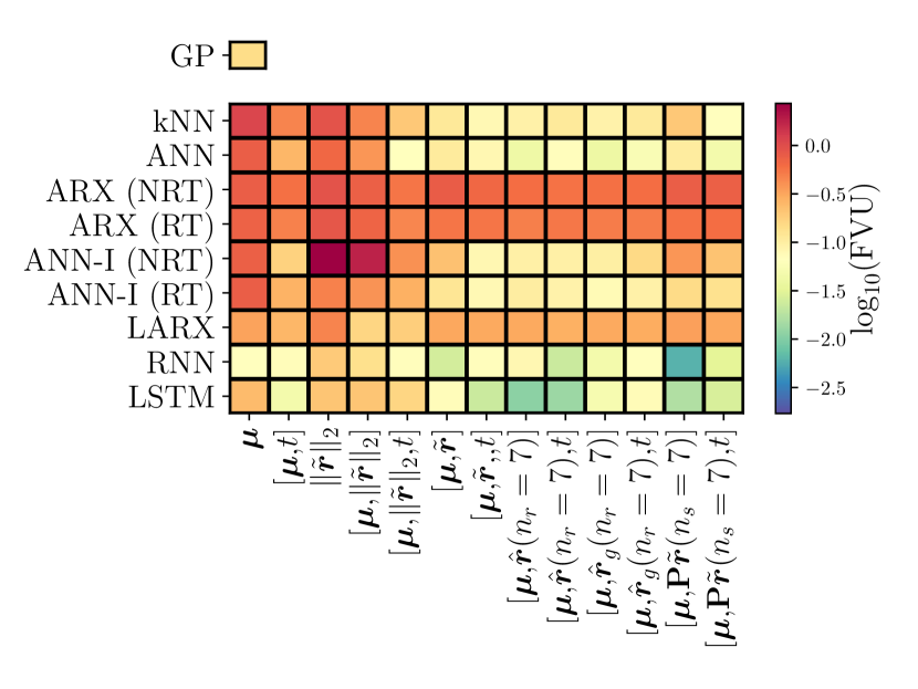
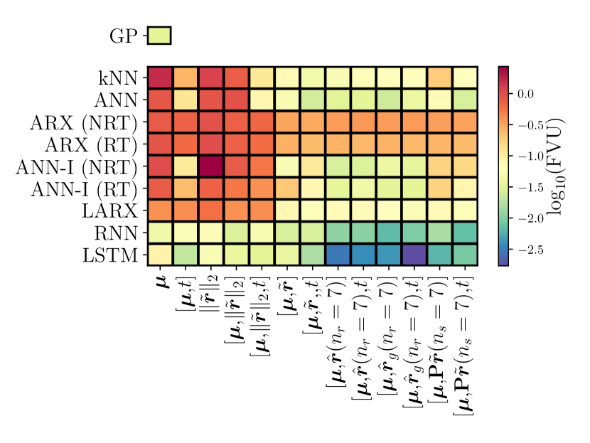
Figure 6 summarizes the performance of each regression method for each feature engineering method for the $\text{Card}({\mathcal{D}_{train}})=50$ case. Feature engineering methods employing the parameters residual-based features provide the best performance across all regression methods. The inclusion of time as a feature is seen to, in general, slightly improve the predictions.

Figures 7 shows the true error versus predicted error for each regression method using the best performing feature method for the $\text{Card}({\mathcal{D}_{train}})=50$ case. Unlike stationary learning problems, deviations of the predicted error from the true error are seen to be highly correlated. This is a realization of the fact that errors at a given time-step are correlated to errors at previous timesteps. As expected, the predictions from the LSTM networks contain the least scatter and provide the best approximation of the true errors.

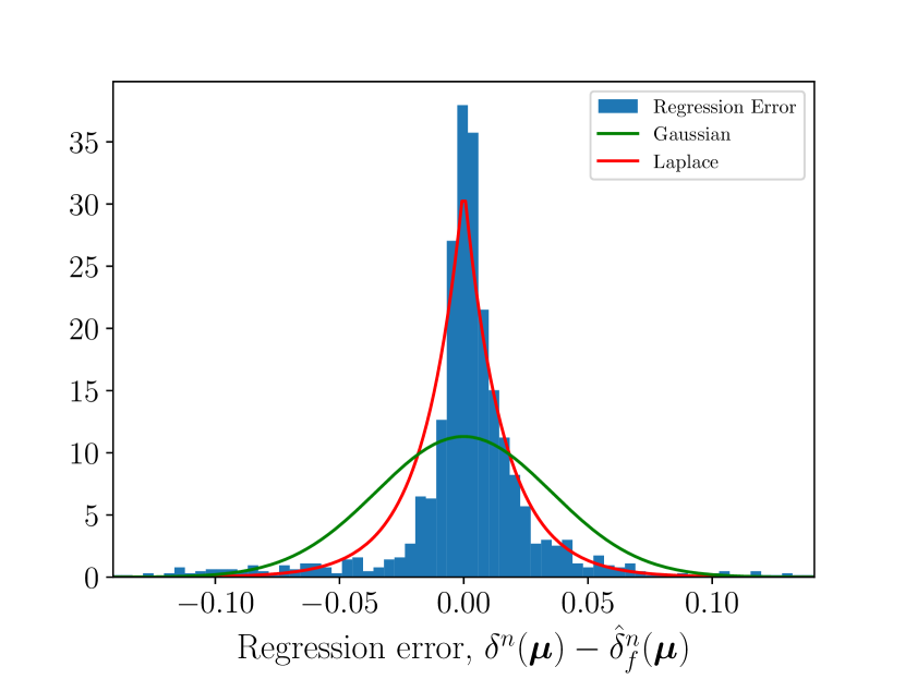
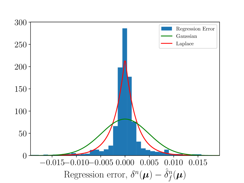
Figures 8 residual distributions of the best forming regression method (LSTM) with the best performing feature method for both the normed state and QoI predictions. The distributions are compared to the assumed Gaussian distribution. Table 3 lists various validation frequencies of the approximated distribution. The true error is observed to contain a slightly sharper distribution than the Gaussian distribution, with longer tails and a more pronounced peak.

$\omega$	$\delta_{\mathbf{u}}$	$\delta_{q}$
0.68	0.681	0.878
0.95	0.861	0.915
0.99	0.945	0.946

Table 3: Validation frequencies of the assumed Gaussian distribution

(a) $\delta_{\mathbf{u}}$, Dataset 1

(b) $\delta_{\mathbf{u}}$, Dataset 2

Figure 5: Fraction of variance unexplained on the test set for different machine learning methods and input features.

(a) $\delta_{\mathbf{u}}$, Dataset 1

(b) $\delta_{\mathbf{u}}$, Dataset 2

Figure 6: Fraction of variance unexplained on the test set for different machine learning methods and input features.

(a) $\delta_{\mathbf{u}}$, Dataset 1

(b) $\delta_{\mathbf{u}}$, Dataset 2

Figure 7: Fraction of variance unexplained on the test set for different machine learning methods and input features.

(a) $\delta_{\mathbf{u}}$, Dataset 1

(b) $\delta_{\mathbf{u}}$, Dataset 2

Figure 8: Fraction of variance unexplained on the test set for different machine learning methods and input features.

4.2 Reduced-Order Modeling of the Shallow Water Equations

The seconds example considers error estimation for reduced-order models of the shallow water equations, which are given by,

$$\frac{\partial h}{\partial t}+\frac{\partial}{\partial x}(hu)+\frac{\partial}{\partial y}(hv)=0,$$

$$\frac{\partial hu}{\partial t}+\frac{\partial}{\partial x}(hu^{2}+\frac{1}{2}gh^{2})+\frac{\partial}{\partial y}(huv)=0,$$

$$\frac{\partial hv}{\partial t}+\frac{\partial}{\partial x}(huv)+\frac{\partial}{\partial y}(hv^{2}+\frac{1}{2}gh^{2})=0,$$

where $g$ is gravity, which we take to be a parameter in the domain $g=U[2,9]$. We consider the domain $[x,y]\in[0,5]\times[0,5]$ with initial conditions of,

$$h_{0}=1+\beta e^{(x-1)^{2}+(y-1)^{2}},u_{0}=0,v_{0}=0,$$

which corresponds to a Gaussian pulse centered at $(1,1)$ with a magnitude of $\beta$.

The full-order model is a third order discontinuous Galerkin method. The domain is partitioned into $16\times 16$ equally spaced elements. Tensor product polynomials of order $p=3$ represent the solution over each element. The total dimension of the full-order model is $N=12288$. Slip wall boundary conditions are used at the edge of the domain. The full-order model is solved with a time-step of $\Delta t=0.01$ for $t\in[0,10]$. Figure LABEL:fig:swe_surf shows elevation surfaces obtained from one such training simulation.

A reduced-order model is constructed by solving the full-order model for a parameter grid of $g=[3,6,9]$ and $\beta=[0.05,0.1,0.2]$. This corresponds to nine total solves of the full-order model. A reduced-basis is constructed by performing POD on the snapshot matrix obtained from stacking the solution snapshots at each time-step for $t\in[0,5]$ for all 9 cases. It is found that 78 POD modes comprise $99\%$ of the solution energy.

4.2.1 Construction of Test and Training Data for Regression Models

This section outlines the construction of the training and testing data. A large-scale dataset, $\mathcal{T}$, is constructed by solving the full-order and reduced-order models for $100$ random samples in the parameter domain. The output of the full-order model is saved every other time-step, creating $400$ data points for each of the 100 samples. Define the data-set by,

$$\mathcal{T}=\bigcup_{\begin{subarray}{c}i=1\end{subarray}}^{100}\bigcup_{\begin{subarray}{c}j=1\end{subarray}}^{400}\mathcal{T}_{i}^{j},$$

where the subscript $i$ denotes the $i_{th}$ sample, the superscript $j$ denotes the $j_{th}$ saved output of the full-order model, and,

$$\mathcal{T}_{i}^{j}=\{\delta_{i}^{j},\mathbf{x}_{i}^{j}\}.$$

A variety of training sets generated from $\mathcal{T}$ are considered:

1. Dataset 1: Every fourth saved-output of the first $50$ samples in $\mathcal{T}$ are set to be the training set, while every fourth saved-output of the last $20$ samples in $\mathcal{T}$ is the testing set,

   $$\mathcal{T}_{train}=\bigcup_{\begin{subarray}{c}i=1\end{subarray}}^{50}\bigcup_{\begin{subarray}{c}j=1\end{subarray}}^{100}\mathcal{T}_{i}^{4j},\qquad\mathcal{T}_{test}=\bigcup_{\begin{subarray}{c}i=81\end{subarray}}^{100}\bigcup_{\begin{subarray}{c}j=1\end{subarray}}^{100}\mathcal{T}_{i}^{4j}.$$

   This data-set tests the ability of the regression methods to predict over time-intervals that are included in the training set. Data points are skipped to have a nominal sequence length of 100 for each parameter instance in the training set.

2. Dataset 2: Every other saved-output for $t<5$ of the first $50$ samples in $\mathcal{T}$ are set to be the training set, while every other saved-output of the last $20$ samples in $\mathcal{T}$ is the testing set,

   $$\mathcal{T}_{train}=\bigcup_{\begin{subarray}{c}i=1\end{subarray}}^{50}\bigcup_{\begin{subarray}{c}j=1\end{subarray}}^{100}\mathcal{T}_{i}^{2j},\qquad\mathcal{T}_{test}=\bigcup_{\begin{subarray}{c}i=81\end{subarray}}^{100}\bigcup_{\begin{subarray}{c}j=1\end{subarray}}^{200}\mathcal{T}_{i}^{2j}.$$

   This data-set tests the ability of the regression methods to predict over time-intervals that are not included in the training set. Data points are again skipped to have a nominal sequence length of 100 for each parameter instance in the training set. Note that in this data-set, the test set has a sequence length of 200 for each parameter instance.

3. Dataset 3: Every other saved-output of the first $50$ samples in $\mathcal{T}$ are set to be the training set, while every fourth saved-output of the last $20$ samples in $\mathcal{T}$ is the testing set,

   $$\mathcal{T}_{train}=\bigcup_{\begin{subarray}{c}i=1\end{subarray}}^{50}\bigcup_{\begin{subarray}{c}j=1\end{subarray}}^{200}\mathcal{T}_{i}^{2j},\qquad\mathcal{T}_{test}=\bigcup_{\begin{subarray}{c}i=81\end{subarray}}^{100}\bigcup_{\begin{subarray}{c}j=1\end{subarray}}^{200}\mathcal{T}_{i}^{2j}.$$

   This data-set tests the ability of the regression methods to predict over time-intervals that are included in the training set. Data points are skipped to have a nominal sequence length of 100 for each parameter instance in the training set.

4. Dataset 4: Every saved-output for $t<5$ of the first $50$ samples in $\mathcal{T}$ are set to be the training set, while every saved-output of the last $20$ samples in $\mathcal{T}$ is the testing set,

   $$\mathcal{T}_{train}=\bigcup_{\begin{subarray}{c}i=1\end{subarray}}^{50}\bigcup_{\begin{subarray}{c}j=1\end{subarray}}^{200}\mathcal{T}_{i}^{j},\qquad\mathcal{T}_{test}=\bigcup_{\begin{subarray}{c}i=81\end{subarray}}^{100}\bigcup_{\begin{subarray}{c}j=1\end{subarray}}^{400}\mathcal{T}_{i}^{j}.$$

   This data-set tests the ability of the regression methods to predict over time-intervals that are not included in the training set. Data points are again skipped to have a nominal sequence length of 100 for each parameter instance in the training set. Note that in this data-set, the test set has a sequence length of 200 for each parameter instance.

It is remarked that, for feature methods 5-9, PCA is performed using only the data in the training set.

4.2.2 Construction of Training Data for Stochastic Error Model

4.2.3 Regression Results

(a) $\delta_{\mathbf{u}}$, Dataset 1

(b) $\delta_{\mathbf{u}}$, Dataset 2

(c) $\delta_{q}$, Dataset 1

(d) $\delta_{q}$, Dataset 2

Figure 9: Fraction of variance unexplained on the test set for different machine learning methods and input features.

(a) $\delta_{\mathbf{u}}$, Dataset 1

(b) $\delta_{\mathbf{u}}$, Dataset 2

(c) $\delta_{q}$, Dataset 1

(d) $\delta_{q}$, Dataset 2

Figure 10: Fraction of variance unexplained on the test set for different machine learning methods and input features.

(a) $\delta_{\mathbf{u}}$, Dataset 1

(b) $\delta_{\mathbf{u}}$, Dataset 2

(c) $\delta_{q}$, Dataset 1

(d) $\delta_{q}$, Dataset 2

Figure 11: Fraction of variance unexplained on the test set for different machine learning methods and input features.

4.2.4 Statistical Error Model

(a) Histogram of regression errors, $\delta_{q}$, overlaid with the predicted Laplacian and Gaussian distributions.

(b) Error in $\delta_{q}$ as a function of time with $1$-sigma limits.

(c) Histogram of regression errors, $\delta_{q}$, overlaid with the predicted Laplacian and Gaussian distributions.

(d) Error in $\delta_{q}$ as a function of time with $1$-sigma limits.

Figure 12: Fraction of variance unexplained on the test set for different machine learning methods and input features.

(a) Histogram of regression errors, $\delta_{q}$, overlaid with the predicted Laplacian and Gaussian distributions.

(b) Error in $\delta_{q}$ as a function of time with $1$-sigma limits.

(c) Error in $\delta_{q}$ as a function of time with $1$-sigma limits.

(d) Error in $\delta_{q}$ as a function of time with $1$-sigma limits.

Figure 13: Fraction of variance unexplained on the test set for different machine learning methods and input features.

4.3 Coarse Solution Prolongation of Burgers’ Equation

The final example considers coarse solution prolongation of parameterized forced Burgers’ equation as given by,

$$\frac{\partial u}{\partial t}+\frac{1}{2}\frac{\partial u^{2}}{\partial x}=\alpha e^{\beta x},$$ (14)

on the spatio-temporal domain $x\in[0,100],t\in[0,40]$. The boundary conditions are given by,

$$u(0,t)=u_{a},\qquad u(x,0)=u_{i}.$$ (15)

The parameter domain is $\alpha\in U[0.005,0.05]$, $\beta\in U[0.005,0.05]$, $u_{i}\in U[0.5,2.5]$, and $u_{a}\in[3,5]$. Error estimation for the quantity of interest $u(50,t)$ is considered.

The full-order model is a finite volume scheme of cell width $\Delta x=0.1$. The Roe flux is used at the cell interfaces. The implicit Euler method with $\Delta t=0.0$ is used for time-discretization.

The coarse-grid solution is a finite volume scheme of cell width $\Delta x=2$. The prolongation operator consists of a linear interpolation of the coarse-grid solution onto the fine grid.

4.3.1 Construction of Test and Training Data for Regression Models

A large-scale dataset, $\mathcal{T}$ is constructed by solving the fine and coarse-mesh solutions for $100$ random samples of the parameter domain. The output of the full-order model is saved at every time-step, creating 800 data points for each of the 100 samples. Define the data-set by,

$$\mathcal{T}=\bigcup_{\begin{subarray}{c}i=1\end{subarray}}^{100}\bigcup_{\begin{subarray}{c}j=1\end{subarray}}^{800}\mathcal{T}_{i}^{j},$$

where the subscript $i$ denotes the $i_{th}$ sample, the superscript $j$ denotes the $j_{th}$ saved output of the full-order model, and,

$$\mathcal{T}_{i}^{j}=\{\delta_{i}^{j},\mathbf{x}_{i}^{j}\}.$$

A variety of training sets generated from $\mathcal{T}$ are considered:

1. Dataset 1: Every eigth saved-output of the first $50$ samples in $\mathcal{T}$ are set to be the training set, while every eigth saved-output of the last $50$ samples in $\mathcal{T}$ is the testing set,

   $$\mathcal{T}_{train}=\bigcup_{\begin{subarray}{c}i=1\end{subarray}}^{50}\bigcup_{\begin{subarray}{c}j=1\end{subarray}}^{100}\mathcal{T}_{i}^{4j},\qquad\mathcal{T}_{test}=\bigcup_{\begin{subarray}{c}i=81\end{subarray}}^{100}\bigcup_{\begin{subarray}{c}j=1\end{subarray}}^{100}\mathcal{T}_{i}^{4j}.$$

   This data-set tests the ability of the regression methods to predict over time-intervals that are included in the training set. Data points are skipped to have a nominal sequence length of 100 for each parameter instance in the training set.

It is remarked that, for feature methods 5-9, PCA is performed using only the data in the training set.

5 Conclusions

Appendix A Keras Algorithms

A.1 Neural Network

⬇

1def build_nn(X,y,neurons,depth,regularization):

model = Sequential()

3 model.add(Dense(neurons,input_shape=(None,np.shape(X)[-1]),activation=’relu’,use_bias=True,kernel_regularizer=regularizers.l2(10.**regularization)))

for i in range(1,depth):

5 model.add(Dense(neurons,activation=’tanh’,use_bias=True,

kernel_regularizer=regularizers.l2(10**regularization)))

7 model.add(Dense(np.shape(y)[-1],activation=’linear’,use_bias=True))

model.compile(loss=’mean_squared_error’, optimizer=’Adam’)

9 return model

Listing 1: Python code for the initialization of the neural networks used in this work.

A.2 Recurrent Neural Network

⬇

1def build_rnn(X,y,neurons,depth,regularization):

model = Sequential()

3 model.add(SimpleRNN(neurons,input_shape=(None,np.shape(X)[-1]),

recurrent_initializer=keras.initializers.Constant(value=0.1),

5 return_sequences=True , kernel_regularizer=regularizers.l2(10**regularization),

recurrent_regularizer=regularizers.l2(10**regularization)) )

7 for i in range(1,depth):

model.add(SimpleRNN(neurons,

9 recurrent_initializer=keras.initializers.Constant(value=0.2),

return_sequences=True,

11 kernel_regularizer=regularizers.l2(10**regularization) ,

recurrent_regularizer=regularizers.l2(10**regularization)) )

13 model.add(Dense(np.shape(y)[-1],activation=’linear’,use_bias=True))

model.compile(loss=’mean_squared_error’, optimizer=’Adam’)

15 return model

Listing 2: Python code for the initialization of the recurrent neural networks used in this work.

A.3 Long Short-Term Memory Network

⬇

1def build_lstm(X,y,neurons,depth,regularization):

model = Sequential()

3 model.add(LSTM(neurons,input_shape=(None,np.shape(X)[-1]), recurrent_initializer=keras.initializers.Constant(value=0.1), return_sequences=True , kernel_regularizer=regularizers.l2(10**reg) , recurrent_regularizer=regularizers.l2(10**regularization)) )

for i in range(1,depth):

5 model.add(LSTM(neurons, recurrent_initializer=keras.initializers.Constant(value=0.2), return_sequences=True , kernel_regularizer=regularizers.l2(10**reg) , recurrent_regularizer=regularizers.l2(10**regularization)) )

model.add(Dense(np.shape(y)[-1],activation=’linear’,use_bias=True))

7 model.compile(loss=’mean_squared_error’, optimizer=’Adam’)

return model

Listing 3: Python code for the initialization of the LSTM networks used in this work.