First ALMA Millimeter Wavelength Maps of Jupiter, with a Multi-Wavelength Study of Convection

Abstract

We obtained the first maps of Jupiter at 1–3 mm wavelength with the Atacama Large Millimeter/Submillimeter Array (ALMA) on 3–5 January 2017, just days after an energetic eruption at 16.5^∘S jovigraphic latitude had been reported by the amateur community, and about 2-3 months after the detection of similarly energetic eruptions in the northern hemisphere, at 22.2–23.0^∘N. Our observations, probing below the ammonia cloud deck, show that the erupting plumes in the SEB bring up ammonia gas from the deep atmosphere. While models of plume eruptions that are triggered at the water condensation level explain data taken at uv–visible and mid-infrared wavelengths, our ALMA observations provide a crucial, hitherto missing, link in the moist convection theory by showing that ammonia gas from the deep atmosphere is indeed brought up in these plumes. Contemporaneous HST data show that the plumes reach altitudes as high as the tropopause. We suggest that the plumes at 22.2–23.0^∘N also rise up well above the ammonia cloud deck, and that descending air may dry the neighboring belts even more than in quiescent times, which would explain our observations in the north.

1 Introduction

Numerous ground-based and space-borne telescopes have monitored Jupiter closely during the past few years, being motivated to provide support to NASA’s Juno mission, in particular during close encounters of the spacecraft with Jupiter, referred to as Perijoves (PJs). Although Juno data are not included in this paper, the observations discussed were similarly motivated. They were carried out in early January 2017, near Juno’s originally planned PJ8 (which was 11 Jan. 2017). Contributing uniquely to this campaign, observations were obtained with the Atacama Large Millimeter/Submillimeter Array (ALMA). This is the first time that ALMA observed Jupiter’s atmosphere at 1.3 and 3 mm (233 and 97 GHz), probing 40-50 km below the visible ammonia-ice cloud (down to 3-4 bar). Data at these wavelengths complement the Very Large Array (VLA) Jupiter maps of 2013-2014 in the cm wavelength range (de Pater et al., 2016, 2019; henceforth dP16 and dP19, respectively).

Fortuitously, the timing of the ALMA observations was just a few days after amateur astronomer Phil Miles announced the onset of an “outbreak” in Jupiter’s South Equatorial Belt (SEB; 7–20^∘S): a small bright white plume at 16.5^∘S that signified the start of a large-scale disruption in the SEB (Fig. 1). The last full fade and revival cycle of the SEB took place in 2009-2011 (Fletcher et al., 2011; 2017a), where the word “fading” is used when the SEB looses its brown color and turns white (like a lighter-colored axisymmetric band, referred to as a “zone”). Although the present outbreak was not preceded by a period of fading, there are many similarities between this outbreak and the revival cycle following the 2009-2011 fade, as shown in this paper. While outbreaks in the SEB occur at irregular intervals of a few years, periods between faded states can be over three decades long (Rogers, 1995; Fletcher, 2017).

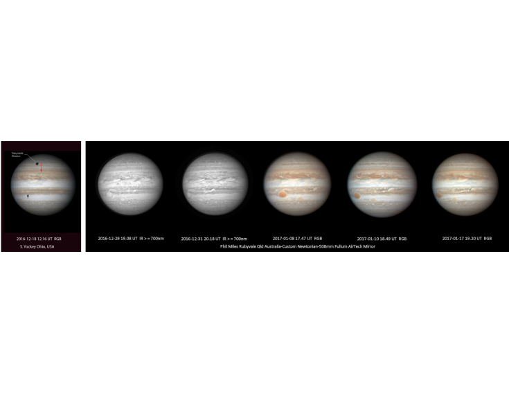
Figure 1: Images in visible light spanning the origin of the SEB outbreak. A pre-outbreak image on 28 Dec. 2016; discovery image on 29 Dec. 2016; and subsequent images on 31 Dec. 2016, and 8, 10 and 17 Jan. 2017. The source of the Outbreak remains fixed near 208^∘ System II, and the disturbance propagates to the east, as shown by the sequence of images. (Courtesy S. Yockey, Ohio, USA; Phil Miles, Australia).

Meanwhile, in the northern hemisphere, three months prior to our observations, four extremely bright white plumes had been discovered at 22.2–23.0^∘N, i.e., just south of the North Temperate Belt (NTB; 24–31^∘N). Over the next few months this led to a planetary-scale disturbance in the NTB, resulting in a uniform orange belt by the end of November 2016, at latitudes spanning 22.8–26.7^∘Nke (Sánchez-Lavega et. al., 2017). Such NTB outbreaks occur on timescales $\gtrsim$5 years.

Radio observations at mm–cm wavelengths are unique because they probe below the visible cloud deck (dP19). Therefore, our ALMA data give a unique perspective on the SEB outbreak and the aftermath of the NTB revival since these are the only data that let us trace these events below the ammonia cloud deck. In the case of the NTB, our data were acquired after the entire belt had “revived”, but in case of the SEB the data were taken during the period when plume eruptions were in progress.

We present the observations in Section 2, the results in Section 3 with models in Section 4, concluding with a discussion and a possible explanation in the context of moist convection theory in Section 5. A brief summary is provided in Section 6.

2 OBSERVATIONS

Jupiter was observed with ALMA on 3-5 January 2017, when the array was composed of 40 antennas, and placed in a relatively compact configuration (C40-2). Observations were obtained in Band 3 (3 mm, 90–105 GHz) and Band 6 (1.3 mm, 223–243 GHz). The observations are summarized in Table 1.

Quasi-simultaneous observations were obtained at several other telescopes on January 10–14. Specifically, observations at a spatial resolution 3.5–4 times higher than that of the 1.3 mm ALMA data were obtained with the Very Large Array (VLA) in the X-band ($\sim$3.5 cm, 8–12 GHz); although the spatial resolution in these maps is exquisite, the large scale structure is poorly mapped. We used the Hubble Space Telescope (HST) WFC2/UVIS camera at multiple wavelengths to map the visible cloud structure, including bright plumes. With the Gemini telescope we imaged the planet at a wavelength of 5 $\mu$m using the NIRI instrument, while we simultaneously obtained 5-$\mu$m spectroscopic data with the Keck telescope using the NIRSPEC spectrometer, both probing down to 7–8 bar in cloud-free regions. To diagnose thermal effects of the SEB outbreak on the upper troposphere and stratosphere, we used mid-infrared detectors on the Very Large Telescope (VLT), VISIR, and Subaru telescope, COMICS. Table 2 provides a summary of all observations taken in addition to the ALMA data. In the following subsections we describe each of the observations in more detail.

2.1 ALMA

We obtained 5 – 6 observations (or “executions”) with ALMA (program 2016.1.00701.S) on each of the first two days (3 and 4 Jan. 2017), interleaving Band 3 (3 mm, 90–105 GHz) and Band 6 (1.3 mm, 223–243 GHz); one additional observation was taken on 5 Jan. Since Jupiter is large, roughly 35${}^{\prime\prime}\;$across during the observing period, we used the mosaicing method to map the entire planet. A total of 5 pointings were used in Band 3, and 17 in Band 6, so that the majority of time was spent in Band 6. In each setup, we had 4 spectral windows, each 2 GHz wide.

The basic data received from an interferometer array, such as the VLA or ALMA, are (complex) visibilities, formed by correlating signals from the array’s elements. These are measured in the u-v plane, where the coordinates u and v describe the separation, or baseline, between two antennas (i.e., an interferometer) in wavelength, as projected on the sky in the direction of the source. We refer the reader to de Pater et. al. (2019) for a summary of this technique.

The initial flagging and calibration was done using the ALMA pipeline in the Common Astronomy Software Applications package, CASA. Unfortunately, the absolute flux density of Jupiter in the various observations was obtained using different flux calibrators, which resulted in slightly different flux scales between executions. For all observations J1256-0547 was used as phase calibrator. We modified the flux densities so that all scans were referenced to Callisto, for which we used the internal model in CASA (Butler-Horizons 2012). We modified the phases of Jupiter to take out its motion across the sky. The MIRIAD software package (Sault et al., 1995) was used to create maps of the planet . ALMA’s primary beam was assumed to be a gaussian with FWHM $1.13\lambda/D$ radians ($\lambda=$ wavelength; $D=$ diameter ALMA dish, which we assumed to be 12 m). The procedures to produce longitude-smeared and longitude-resolved maps were then similar to those used in earlier VLA observations, including self-calibration (Sault et al., 2004; dP16, dP19). However, the techniques were generalized to account for beam effects and mosaicking. Due to the excellent u-v-coverage in ALMA data compared to the VLA, the maps are essentially devoid of instrumental artefacts.

As in the previous papers, in order to best assess small variations on Jupiter’s disk, a limb-darkened disk was subtracted from the u-v data with a brightness temperature and limb-darkening parameter that produced a best fit (by eye) to the data (i.e., “best fit” means parameters such that there is no planet after imaging the residual u-v data). Limb-darkening was modeled by multiplying the brightness temperature at disk center, T${}_{b}^{\prime}$, by (cos$\theta$)^q, with $\theta$ the emission angle on the disk (i.e., the angle between the surface normal vector and the line-of-sight vector to Earth), and $q$ a constant that provides a best fit to the data. Although more complex limb-darkening models could be used instead of our simple algorithm, our main goal is to subtract the large bright smoothly-varying structure that is Jupiter’s disk, so we can produce reliable maps of the residuals. The subtracted disk is added back before we model the data with radiative transfer calculations (see also dP19).

Disks which provided a best-fit to the Band 3 (T${}_{b}^{\prime}=$ 131 K with $q=$ 0.10) and Band 6 (T${}_{b}^{\prime}=$ 115 K with $q=$ 0.08) data revealed brightness temperatures that were only of order 60–70% of what we expected. Although our data lacked short spacings, (in Cycle 4 it was not possible to simultaneously use the Atacama Compact Array (ACA) and the 12-m array), this was not the reason for the low observed brightness temperatures. These appear to be caused by errors in the ALMA observations and pipeline reduction software. Based on an ALMA memo on calibration, we conclude that the system temperature, Tsys, is usually determined on blank sky. This is reasonable for a source which does not contribute significantly to Tsys. However this approach is not appropriate for very bright sources. For example for ALMA observations of the Sun, Tsys is determined on the disk of the Sun. A similar approach should be used when observing the bright planets as well.

In order to remedy this shortcoming, we assumed disk-averaged brightness temperatures based on the best model fits to dP19’s disk-averaged brightness temperature spectrum (Fig. 4 in dP19, with the Karim et al. (2018) model), and scaled the data accordingly. The values used are listed in Table 3, T_b(adopt). We then calculated the brightness temperature at disk center, T_b(cent), that would provide T_b(adopt) when using the limb-darkening parameter $q$, and after subtracting the cosmic microwave background (T_cmb) to mimic the observations. After putting the originally subtracted disk back, we multiplied the maps by T_b(cent)/T${}_{b}^{\prime}$ and added T_cmb to match the observations as close as possible to Jupiter’s disk.

2.2 VLA

Jupiter was observed with the VLA (program 16B-048) on 11 Dec. 2016 and 11 Jan. 2017. Observations were obtained in the X band (8–10 GHz in 2016; 8–12 GHz in 2017), while the VLA was in its most extended (A) configuration. The VLA data were processed using the standard pipeline; the data were averaged in time (10s) and in frequency (8 channels) and remaining noisy baselines were removed manually. The dataset was reduced using the full 2 or 4 GHz bandwidth and additionally, the data were split spectrally into 1-GHz wide sets and each set was self-calibrated once on a limb-darkened model with brightness temperature and limb-darkening coefficient obtained from dP16. After subtracting the aforementioned model, longitude-resolved images were formed using the MIRIAD software package (Sault et al., 2004; dP16, dP19). Details on the observations are provided in Tables 2 and 3.

2.3 HST

Images in the UV/visible/near-IR range were taken on 11 Dec. 2016 (program GO-14661) and 11 Jan. 2017 (program GO-14839 ) with the UVIS detector of the WFC3 instrument aboard the Hubble Space Telescope (Dressel 2019; see their Table 6.2 for filter properties). Raw data are available from the Hubble MAST archive, and processed data are available from https://archive.stsci.edu/prepds/wfcj.

Corrections were applied for fringing at long wavelengths (Wong, 2011), and cosmic ray hits were removed based on their sharpness (van Dokkum, 2001). The images were navigated by aligning the data to a synthetic limb-darkened disk, as described in Lii et al. (2010).

2.4 VLT

Thermal-infrared observations in eight narrow-band filters between 7-20 $\mu$m were acquired by the VISIR instrument, with a 9^th band covering the 5-$\mu$m window (Lagage et al., 2004) on the VLT on 15-17 Dec. 2016 (program 098.C-0681(C)) and on 10-11 Jan. 2017 (program 098.C-0681(D)), continuing the sequence of Juno-supporting observations that had started in Feb. 2016 (described in Fletcher et al., 2017b). The eight filters are selected to provide constraints on upper tropospheric (8–600 mbar) and stratospheric (10–20 mbar) temperatures, along with distributions of 500-mbar aerosols and ammonia gas. Although these observations were not global in extent, they were designed to capture two separate hemispheres on two separate nights. VLT’s 8-m primary mirror provided diffraction-limited spatial resolutions of 0.25-0.8^′′. Standard image reduction procedures were used (Fletcher et al., 2009), including despiking and destriping to remove detector artefacts, limb fitting to assign geometric information to each pixel, cylindrical reprojection, and absolute radiometric calibration via comparison to Cassini Composite Infrared Spectrometer (CIRS) observations.

2.5 Subaru

Images of Jupiter at 7-20 $\mu$m were acquired using the COMICS instrument at the Subaru telescope between January 11 and 14, 2017 (UTC) (Kataza et al., 2000). Subaru’s 8-m primary aperture provides a similar spatial resolution as the VLT at the same wavelengths. A 2$\times$1 dithering of the COMICS field-of-view ($\sim$45^′′$\times$32^′′) was performed in order to map the entire jovian disk ($\sim$37^′′) while avoiding detector artefacts at the edges of the field. The reduction of images was performed using the same procedures as described above for the VLT/VISIR data. Images recorded over the four consecutive nights were stitched together to produce an image over 360^∘ in longitude.

2.6 Gemini

Thermal infrared images were taken with the NIRI instrument at Gemini North Observatory in the 5-$\mu$m wavelength range (Hodapp et al. 2003). We use the M’ filter, with a central wavelength of 4.68 $\mu$m, and the f/32 camera with its 22.4${}^{\prime\prime}\;$square field of view. Data were acquired on 2017-01-11 (program GN-2016B-FT-18), and are available from the Gemini archive at https://archive.gemini.edu/.

Images were mapped into the latitude/longitude coordinate space by aligning the data with a synthetic wire-frame disk, and stacked in the latitude/longitude coordinate space to avoid errors that would be introduced by coadding images of a rotating planet. A “lucky imaging” approach was used, taking many 0.3-sec exposures and coadding only the sharpest individual frames. The full data reduction pipeline is described by Wong et al. (2019).

2.7 Keck

We obtained 5-$\mu$m spectra of Jupiter using NIRSPEC, which is an echelle spectrograph on the Keck 2 telescope, with 3 orders dispersed onto a 1024$\times$1024 InSb array (McLean et al 1998). A 0.4^′′$\times$24${}^{\prime\prime}\;$slit was aligned north-south on Jupiter at two longitudes east of the SEB source outbreak, resulting in spectra with a resolving power of 20,000. The spectra were obtained on January 11, 2017 (program 2016B_-N045NS). The geocentric Doppler shift at this longitude was -31.5 km/sec. The water vapor abundance above Mauna Kea was 2.5 precipitable mm along the line of sight to Jupiter, or 1.7 precitable mm in a vertical column. This was derived from fitting telluric lines in both stellar and Jupiter spectra.

3 Results

3.1 Longitude-smeared ALMA Maps

Figure 2 shows longitude-smeared maps of Jupiter (panel B), averaged over the entire Band 3 (3 mm) and (separately) Band 6 (1.3 mm). Similar to the longitude-smeared VLA maps taken in December 2013 (top image), we see numerous bright and dark bands across Jupiter’s disk, in particular at 1.3 mm where the spatial resolution in the north-south direction is similar to that of the 2013 VLA data (Table 3). The radio-hot belt at 8.5–11^∘N latitude, near the interface between the North Equatorial Belt (NEB; 7–17^∘N) and the Equatorial Zone (EZ; 7^∘S–7^∘N) is prominent, as well as the minimum in brightness temperature (T_b) near a latitude of 4^∘N, i.e., in the EZ.

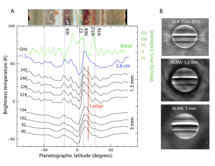
Figure 2: A) North-south scans through longitude-smeared ALMA and VLA maps. The scans were created by median averaging over 60^∘ of longitude, centered on the central meridian of each map, after reprojection on a longitude/latitude grid. Since a limb-darkened disk had been subtracted from the data, the background level of each scan is centered near 0 K, as for the 224 GHz scan. The scans are offset for clarity by 10 K each, while each set is separated by 20 K. The spatial resolution of the 3-mm maps is about 2.5 times lower than at 1.3 mm and the VLA maps, which lowers the feature contrast. The vertical dashed lines (at e.g., the EZ, SEB, NEB and NTB) help guide the eye to line up features. The green line at the top is the (eastward) wind profile as measured from the HST data; the scale is given on the right side. At the top we show a slice through the HST image from Figure 4. B) Longitude-smeared ALMA maps of Jupiter’s thermal emission at 1.3 and 3 mm (averaged over the entire Bands 6 and 3, resp.), and a VLA 3-cm map from dP19, after subtraction of a limb-darkened disk.

We reprojected each 2-GHz wide spectral window map on a longitude/latitude grid, and constructed north-south scans through each of the maps, which are shown in panel A of Figure 2, together with a VLA scan from 2013 at 2.6 cm (dP19) which probes similar depths as the ALMA scans (see below). The background level curves upwards at higher latitudes, because the poles are less limb-darkened than east-west scans along the planet, as shown before from VLA maps (de Pater, 1986; dP19) and Cassini radiometer data (Moeckel et al., 2019). The top-most green curve is the wind profile as measured from the HST data (11 January 2017), using the methodology of Asay-Davis et al. (2011) and Tollefson et al. (2017). A strip through the HST map (Section 3.2) is shown at the top of the figure.

Ammonia gas is the dominant source of opacity over the entire mm–cm wavelength range, so our maps can be used to derive the 3-dimensional distribution of this gas (as in dP16, dP19). Since the 1–3 mm and 2.5–3 cm spectral ranges are on opposite sides of the NH₃ absorption band, and have a similar absorption strength, the two wavelength ranges probe the same depths in Jupiter’s atmosphere ($\sim$0.5–4 bar) as shown by disk-averaged spectra (Fig. 4 in dP19) and the weighting functions (Fig. 3). Despite the 3-year separation between the 2013 VLA and ALMA data, the similarity between the VLA 2.6 cm and ALMA 1.3 mm scans (at a similar spatial resolution) is striking. The contrast between the minimum (EZ) and maximum (radio-hot belt, i.e., NEBs) brightness temperatures in the ALMA maps varies from 22 to 27 K from 3 mm down to 1.3 mm (Fig. 2), which is the same as measured with the VLA at 2.5–3 cm (Fig. 7 in dP19). In addition, the zone-belt structure in the southern hemisphere shows an excellent match between the 2013 VLA and ALMA scans. This shows that, averaged over longitude, the southern hemisphere has remained the same over a 3-year period (12/2013–1/2017).

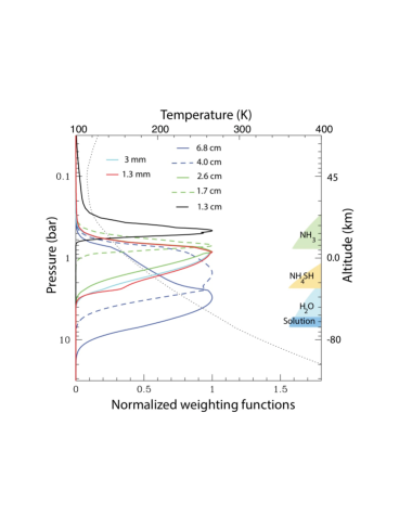
Figure 3: The temperature profile (dotted line; wet adiabat) and weighting functions for our nominal atmosphere in thermochemical equilibrium, under nadir viewing conditions. In our nominal atmosphere the abundances of CH₄, H₂O, and Ar in the deep atmosphere are enhanced by a factor of 4 over the solar values, and NH₃ and H₂S are enhanced by a factor of 3.2 each. On the right-hand side we indicate the various cloud layers expected to form in thermochemical equilibrium. The weighting functions move down in the atmosphere if there is less NH₃ gas, such as in the NEB.

The situation is different in the northern hemisphere. Near 17–18^∘N latitude, there is a “ledge” (i.e., a plateau with an abrupt drop-off) in the ALMA profile that is missing in the 2013 VLA data. Moreover, the ALMA data show a clear minimum in T_b at $\sim$23^∘ in the North Tropical Zone (NTrZ; 17–24^∘N), just south of the prominent eastward jet; such a clear minimum is not seen in the 2013 VLA data. In the visible, the NTrZ is usually white, indicative of upwelling gases. At present, as shown in the HST strip above the scans, the NTrZ is highly disturbed (and in part colored orange). A comparison between the ALMA scans and the HST strip further shows that subtle variations in T_b match variations in color in the HST data, which implies that changes in the visible are related to latitudinal variations in the ammonia abundance below the cloud deck. This is also interesting, because it is well known that colors of Jupiter’s bands change temporally (e.g., fading of the SEB, expansions of the NEB, and the color change in the NTrZ in Fig. 2A), while the wind profile (at the NH₃ cloud deck) is very stable (except for changes in the absolute velocity of the 24^∘ eastward jet) (e.g., Rogers, 1995; Asay-Davis et al., 2001; Tollefson et al., 2017).

3.2 Longitude-resolved Maps at Radio, Visible and Mid-Infrared Wavelengths

A plethora of structure is seen in the ALMA disk-resolved maps, as shown most clearly in the 1.3-mm maps, Figure 4A. Bright areas indicate a higher brightness temperature, assumed to be caused by a lower NH₃ abundance (as in dP19, assuming the temperature profile follows an adiabat), and dark areas indicate a lower brightness temperature, caused by a higher opacity in the atmosphere. The radio-hot belt at 8.5–11^∘N latitude (NEBs) contains prominent hot spots with small well-defined dark regions interspersed. The dark regions are small plumes of NH₃ gas, which are likely associated with the small bright clouds in the HST map (green arrows, #6, in Fig. 4B) at similar latitudes ($\sim$12^∘N). Just to the south are larger dark and somewhat oval-shaped regions; these are the plumes of ammonia gas that were most striking in VLA data at $\sim$6 cm wavelength (dP16) but were visible at all radio wavelengths observed (1–13 cm) (dP19), as well as in the thermal infrared as indicated in Figure 5, in particular near 10 $\mu$m (Fletcher et al., 2016). The Great Red Spot (GRS) in the ALMA map is a well-defined structure surrounded by a bright ring, and a turbulent wake to the west. Oval BA is not visible, likely due to the absence of the, apparently transient, bright ring around the feature and westward wake, which made it visible in the 2013-2014 VLA data (dP16, dP19). A small cyclonic vortex can be discerned to the west of Oval BA, that is bright at radio wavelengths and at 5 $\mu$m (see Fig. 6), indicative of NH₃-dry air and a clearing of aerosols. The anticyclonic vortices at 40^∘S are characterized in the radio and mid-infrared by a darker center surrounded by brighter areas. The dynamics of these small vortices as seen at 5 $\mu$m was discussed by de Pater et al. (2010; 2011). The HST and mid-infrared data were taken $\sim$1 week after the ALMA observations. The colored line on the HST panel traces Jupiter’s wind profile, and hence aids both in identifying how much features have moved, and to distinguish latitudes of cyclonic from anticyclonic wind shear.

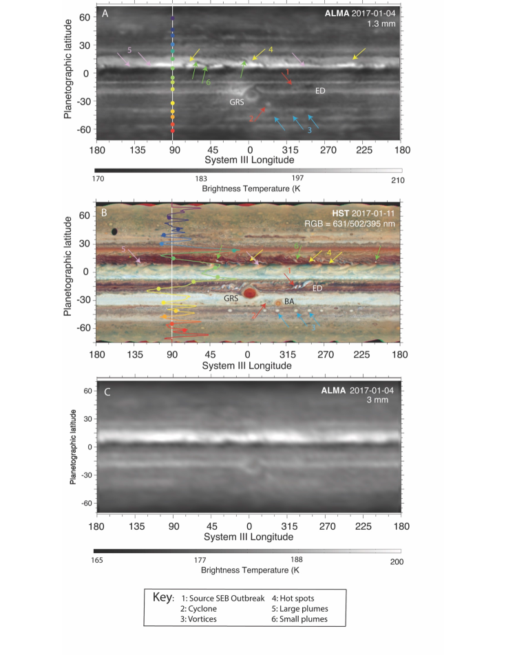
Figure 4: a) ALMA map at 1.3 mm, constructed from data taken 3-5 Jan. 2017. b) HST map from 11 Jan. 2017, with the zonal wind profile superimposed. c) ALMA map at 3 mm, constructed from data taken 3-5 Jan. 2017. Various features are indicated, such as the iconic GRS and Oval BA. Features 1–6, indicated by different colored arrows with numbers, are indicated in the Key. Since features move at different speeds across Jupiter’s disk, and the ALMA and HST observations were taken on different days, we indicate on the HST panel how features at different latitudes (colored dots) have moved since the ALMA data were taken.

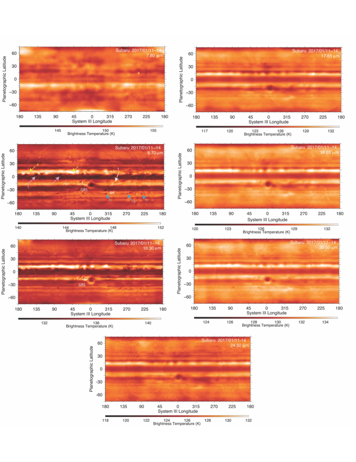
Figure 5: Subaru/COMICS maps at wavelengths of 7.8–24 $\mu$m. Several features are indicated on the 8.70-$\mu$m map, with the same Key as in Fig. 4.

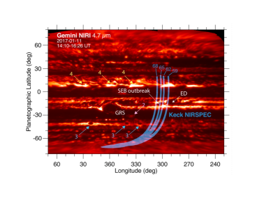
Figure 6: A 4.7-$\mu$m map of Jupiter constructed from images taken by Gemini/NIRI on 11 Jan. 2017. The NIRSPEC slit positions are projected onto the map; the data at the two telescopes were taken simultaneously. We analyzed the ground tracks denoted 59 and 65 in Section 4.4. The numbers with arrows refer to the same Key as in Fig. 4.

4 Radiative Transfer (RT) Models

In the following we discuss radiative transfer (RT) model results of our different observations. We start with general model results for the ALMA data, including the SEB outbreak, and then present more specific calculations at visible and 5 $\mu$m wavelengths with regard to the SEB outbreak.

4.1 RT Modeling of the ALMA Longitude-smeared Maps

We model our data with the RT code Radio-BEAR (Radio-BErkeley Atmospheric Radiative transfer), described in detail in de Pater et al. (2005; 2014; 2019). As in dP19, in our nominal atmosphere, assumed to be in thermochemical equilibrium, the abundances of CH₄, H₂O, and Ar in the deep atmosphere are enhanced by a factor of 4 over the solar values, and NH₃ and H₂S are enhanced by a factor of 3.2, and the temperature-pressure (TP) profile follows an adiabat (typically wet in zones, dry in belts), constrained to be 165 K at the 1 bar level to match the Voyager radio occultation profile (Lindal, 1992). At pressures $\lesssim$0.7 bar, the TP profile follows that determined from mid-infrared (Cassini/CIRS) observations (Fletcher et al., 2009).

As discussed in dP19, variations in the observed brightness temperature can in principle be caused by variations in opacity or by spatial variations in the physical temperature. They show that variations in opacity are much more likely than changes in temperature, and therefore, like in dP19, we attribute all changes to variations in opacity. The latter authors also investigated the effect on the brightness temperature due to changes in the TP profile at and above the ammonia clouddeck, as sensed at mid-infrared wavelengths. After changing the TP profile at each latitude to that observed by Cassini/CIRS (Fletcher et al., 2016), they showed only small changes (varying from zero to perhaps up to maximal 5 K in brightness temperature at some latitudes) near the center of the ammonia absorption band, between 18 and 26 GHz ($\sim$1.3 cm). At deeper levels below the NH₃ cloud, an equatorial thermal wind analysis constrained by Galileo Probe vertical wind shear (Atkinson et al. 1998, Marcus et al. 2019) suggested that there may be horizontal temperature variations of $<$ 3 K between the equator and 7.5 N. Our analysis of ALMA data did not consider small horizontal temperature differences of this magnitude, particularly since vertical wind shear cannot be measured in the region of the SEB outbreak.

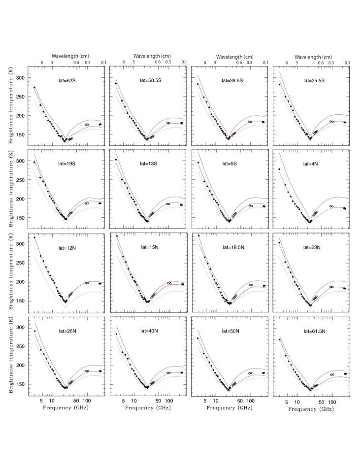
Figure 7: Longitude-averaged brightness temperatures T_b (black dots) from the VLA 2013-2014 data (3–37 GHz, 10–0.8 cm) and the ALMA data (90–242 GHz; 3–1.3 mm) with superposed the best-fit model spectra as derived from the VLA data (dP19: red lines) for several latitudes. The data at $\sim$30–100 GHz (1–0.3 cm; open circles) have a roughly 3–4 times lower spatial resolution than at other frequencies. The cyan and blue curves on all panels show the models with the parameters (NH₃ profiles) that gave best fits to the 2013-2014 VLA EZ and NEB data. (the red curve coincides with the cyan at 4.0N, and with the blue one at 12.0N latitude). The spread between data points is a good estimate for uncertainties in the data.

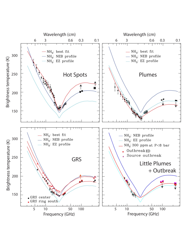
Figure 8: Spectra are shown for various features: hot spots, large plumes, the GRS (center and ring south of the GRS), little plumes and the SEB outbreak, with superposed models that gave best fits to the VLA data of the hot spots, GRS, and plumes (red curves). The ammonia abundances for all models were shown in dP19. The cyan and blue curves on all panels show the models with the parameters (NH₃ profiles) that gave best fits to the 2013-2014 VLA EZ and NEB data. The red curve for the SEB Outbreak data is one where the NH₃ abundance at $P<8$ bar has been replaced by 300 ppm, and following the saturated vapor curve (with a 1% relative humidity) where appropriate.

To examine the 3-dimensional distribution of ammonia gas, or more specifically to identify changes in this distribution since December 2013, we compare in Figure 7 the brightness temperature of the 1–3 mm ALMA data with best-fit models to the 2013-2014 VLA data (from dP19). We stress here that no new models were produced; the existing models were merely extended into the mm-wavelength range. Hence, as in dP19, we ignored opacity by clouds. The latter authors justified this assumption based upon disk-averaged spectra at mm–cm wavelengths. They argued that, if cloud opacity is important, the brightness temperatures at mm wavelengths should be affected much more than in the cm range, since the mass absorption coefficient is inversely proportional to wavelength for particles that are small compared to the wavelength (Gibson et al., 2005).

Figure 7 shows the zonal-mean brightness temperature spectra of the ALMA data together with the corresponding 2013-2014 VLA data, superposed on the models that gave a best fit to the 2013-2014 VLA data at the different latitudes. For comparison we show in all plots the best fits to the EZ (cyan) and NEB (radio-hot belt; blue), while the best-fit VLA models are shown in red. The 3-mm data, with a 2.5–3 times lower spatial resolution, show lower limits to brightness temperatures where maxima in T_b are measured, and upper limits where T_b minima are recorded. As shown, the ALMA data show a near-perfect match to the red curves, except perhaps at the highest latitudes. The brightness temperatures at these high latitudes might be slightly too high due to the bowl-like structure under the planet as introduced by missing short spacings (e.g., de Pater et al., 2001; dP19).

We note that in particular in the EZ (4^∘N), NTrZ (23^∘N), and at latitudes 30–40^∘N and S the ALMA data match the VLA models perfectly, which would corroborate dP19’s assumption that clouds do not affect Jupiter’s brightness temperature at mm-cm wavelengths. To check this statement, we performed several RT calculations. These show that in the NH₃-rich EZ, contribution functions peak at such high altitudes that clouds do not affect the modeled brightness temperature at mm wavelengths. In the NEB, mm-wavelength observations can penetrate to the level of the NH₄SH cloud. We tested one case with high NH₄SH mass loading ($\sim$1.6 g cm^-2 between 2.4 and 0.9 bar) (the water cloud has no effect at mm wavelengths). Although NH₄SH cloud opacity lowered brightness temperatures by a few degrees at mm wavelengths, an extremely strong updraft (length scale $\sim$30 km; see Wong et al., 2015) would be required to generate this much cloud mass. The low NH₃ abundance in the NEB, down to over the 20 bar level (dP16; dP19; Li et al., 2017), is suggestive of subsiding rather than rising air, which makes the presence of such a thick NH₄SH cloud layer quite unlikely. We therefore interpret deviations in the ALMA data compared to the model spectrum in terms of variations in the NH₃ abundance, and ignore potential effects of cloud opacity.

At latitudes 5–13^∘S the ALMA brightness temperatures are slightly lower, so there may have been slightly more NH₃ gas below the cloud layers than in 2013-2014. At 12^∘N the ALMA brightness temperature is a tad too cold, and at 18^∘N and 26^∘N it is slightly warmer than the models, i.e., there seems to be less NH₃ gas at 18^∘N and 26^∘N in 2017 then in 2013-2014. This would explain the observation that the minimum in T_b at 23^∘N appears to be more pronounced in the ALMA data then in the 2013 VLA data (Fig. 2A), since the NH₃ at latitudes north and south of 23^∘N have changed, while the NH₃ abundance stayed constant at 23^∘N.

4.2 RT Modeling of the ALMA Longitude-resolved Maps

Figure 8 compares several resolved features in the ALMA data to models that best fit the 2013-2014 VLA data (from dP19) for the same type of features; as for Figure 7, these models were obtained with our RT code Radio-BEAR. The red curves show the best fit models to the VLA data, and the cyan and blue curves show the best fits to the longitude-smeared EZ and NEB, respectively. In order to properly compare the ALMA data to the models, however, we need to take into account the spatial resolution of the data. For the VLA 2–4 cm data, this varied roughly from 1000$\times$1000 to 2000$\times$2000 km², while the resolution of the 1.3-mm ALMA data is $\sim$2000$\times$4000 km², and for the 3-mm data it is 2.5 times lower still ($\sim$5000$\times$8600 km²) (Table 4). As shown, the model for the center part of the GRS, which is quite extended, fits the ALMA data very well, and the ALMA 1.3 mm data for the bright ring on the south side of the GRS also agree well with the model. As expected, the brightness temperatures of the latter at 3 mm, like at 0.9 cm (30-35 GHz), are too cold compared to the models because the ring is not resolved in these observations. Similarly, the Hot Spots indicate too low a T_b at both 1.3 and 3 mm, and too high a T_b for the plumes. We also indicate the T_b for the source of the SEB outbreak and the disturbance to the east of the outbreak, referred to as the ED (East Disturbance). Because these features are small in angular extent, the measured brightness temperatures should be considered upper limits. We also indicate the values from the January 2017 VLA data (discussed further in Section 5.2), which are well-aligned with the values for the little plumes as measured in the 2013-2014 VLA data. The red curve on this graph is not a best fit; instead, it is a model where the NH₃ abundance was assumed to be 300 ppm at pressures $P<$ 8 bar.

4.3 SEB Outbreak in HST Data

We chose the brightest spot at visible wavelengths as the location of the outbreak (see Fig. 4). The outbreak spectrum was constructed by taking the I/F value at said location in each filter. Background spectra represent the average value of three different locations close to the outbreak. These spectra were fit using our in-house RT code SUNBEAR (Spectra from Ultraviolet to Near-infrared with the BErkeley Atmospheric Retrieval) (Luszcz-Cook, et al., 2016), a python program based on the pydisort module (Ádámkovics et al., 2016). SUNBEAR has been used to model Uranus at IR wavelengths (de Kleer, et al., 2015) and Neptune at UV, Visible, and IR wavelengths (Luszcz-Cook, et al., 2016; Molter, et al., 2019). SUNBEAR takes as inputs the temperature-pressure profile, atmospheric composition as a function of depth, a model of the aerosols, and the gas opacities as a function of temperature and pressure. These inputs are used to construct a model atmosphere, which is fed into pydisort to solve the radiative-transfer equation. Further details on the code can be found in Appendix A of Luszcz-Cook, et al., (2016).

Both the background and outbreak models consist of a variable number of haze layers, an NH₃-ice cloud, and an NH₄SH cloud. The scattering properties of all haze layers were derived from Mie theory, with just the particle size and imaginary refractive index as variable inputs. The fraction of particles with radius $R$, given a peak particle size $r_{p}$, is given by

$$p(R)=\frac{R^{6}e^{\frac{-6R}{r_{p}}}}{\sum_{r=0}^{r=\infty}r^{6}e^{\frac{-6r}{r_{p}}}}$$ (1)

The real part of the refractive index was set to that of ammonia ice, i.e., $1.4$. The clouds were modeled as perfect reflectors with the Henyey-Greenstein asymmetry parameter $g=-0.3$. The NH₃-ice cloud was placed at $0.7$ bar and given an opacity of $10$, while the NH₄SH-ice cloud was placed at $2.5$ bar and given an opacity of $30$. We added four haze layers above the clouds. The topmost haze layer extended from 1 to 100 mbar, the second from 100 to 200 mbar, the third from 200 to 650 mbar, and the fourth from 650 mbar to 700 mbar. We adapted the opacities and particle radii of these haze layers to fit he spectra.

To fit the background spectra, we used an imaginary index of refraction similar to that used for the NEB in Fig. 7 of Irwin et al., (2018). The peak particle radii for the haze layers, which we will refer to as hazes 1–4, with 1 being the uppermost and 4 being the lowermost, were $r_{1}=$0.1 $\mu$m, $r_{2}=$0.3 $\mu$m, $r_{3}=$0.8 $\mu$m, and $r_{4}=$1.0 $\mu$m, The cumulative opacities for each layer were $\tau_{1}=0.1$, $\tau_{2}=0.1$, $\tau_{3}=1.8$, and $\tau_{4}=3.7$.

To match the outbreak spectrum, we used an imaginary refractive index of $4\times 10^{-3}$ in the UV, $7.5\times 10^{-4}$ in the visible, and $2\times 10^{-3}$ in the IR. Using the same haze labeling as the background model, the peak particle radii are $r_{1}=$0.1 $\mu$m, $r_{2}=$0.8 $\mu$m, $r_{3}=$0.3 $\mu$m, and $r_{4}=$0.8 $\mu$m. The cumulative opacities are $\tau_{1}=0.1$, $\tau_{2}=0.2$, $\tau_{3}=0.62$, and $\tau_{4}=0.85$. The results of the radiative transfer modeling of these atmospheres are shown in Figure 9.

We find that the haze above the SEB outbreak has twice the cumulative opacity of the background model at high altitudes (100–200 mbar), but barely a quarter of the cumulative opacity at 0.2–0.7 bar. The outbreak plume also has different scattering properties from the background atmosphere. The imaginary index of refraction is higher for the outbreak, indicating that the hazes are more prone to absorbing light at these wavelengths than the background atmosphere. Finally, we see variations in peak particle radius for each layer that suggests larger particles are being transported to the tropopause from deeper down in the atmosphere, while simultaneously removing larger particles from these deeper hazes.

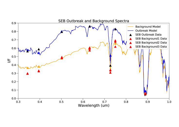
Figure 9: SUNBEAR RT model fit to the SEB outbreak plume and background. The outbreak and background data are shown in black and red, and the respective models are shown in blue and orange. The blue and orange triangles show the model values expected in the HST filters (i.e., model convolved with the HST filter shape).

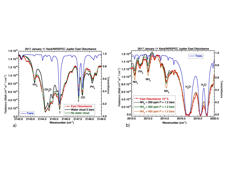
Figure 10: a) Spectrum of Jupiter’s ED compared with synthetic spectra generated from models with (black) and without (green) opaque clouds G at 5 bars. The best fit to the CH₃D feature is for the model without a cloud at the level where water is expected to condense on Jupiter. b) Spectrum of the ED compared with synthetic spectra generated from models with three abundances (200, 300, and 400 ppm) of gaseous NH₃. The best fit model has 300 ppm NH₃. All models have an H₂O abundance of 47 ppm for P $>$ 4.5 bars, consistent with that measured in the Galileo Probe entry site, and no opaque cloud at the 5-bar level.

4.4 Keck 5-$\mu$m Spectroscopy of the SEB Outbreak

In Figure 6, we project the ground tracks of the NIRSPEC slit onto a 4.7-$\mu$m Gemini/NIRI image of Jupiter taken at the same time. We analyzed the tracks denoted 59 and 65, the file numbers of the NIRSPEC spectra. Note that track 59 traverses the western portion of the East Disturbance (ED) at 13^∘S, and track 65 traverses the source region of the SEB outbreak. Both areas are dark at this wavelength due to higher cloud opacity. We analyzed all 3 NIRSPEC orders centered on 4.66, 4.97, and 5.32 $\mu$m. The 4.66-$\mu$m spectrum reveals spectrally resolved absorption features of CH₃D, which were used to derive cloud structure. Spectra at 4.97 $\mu$m show gaseous H₂O and NH₃ absorption features formed between 4 and 6 bars on Jupiter. The 5.32-$\mu$m order samples a strong NH₃ absorption band permitting retrieval of the albedo of the upper cloud layer. In the following we discuss our model fits to the spectra; the details of our methodology are described by Bjoraker et al. (2018).

Figure 10a shows a portion of the spectrum of the ED at 4.66 $\mu$m (2142 to 2149 cm-1). We compare the observed spectrum with a model containing an opaque water cloud at 5 bars, and an alternate model with no cloud opacity at this level. Both models included sunlight reflected from an upper cloud at 600 mbars with an albedo of 12%. This albedo was obtained by fitting the spectrum of the ED in a strong NH₃ band at 5.32 $\mu$m (not shown) where the radiance from the thermal component is expected to be zero. The observed CH₃D absorption feature at 2144 cm^-1 is broader than that in the opaque water cloud model, while the observed line shape is fit quite well by the model lacking a water cloud.

Using a cloud model with a reflecting layer at 600 mbars that is partially transmitting to allow thermal radiation from the deep atmosphere to emerge, we next investigated the abundance of gaseous H₂O and NH₃ by fitting the NIRSPEC spectrum at 4.97 $\mu$m (2010-2020 cm^-1). Since we found no evidence of a water cloud at 5 bars, we adopted the gaseous H₂O profile as measured in the Galileo Probe entry site (Wong et al., 2004). We adjusted one parameter, namely the pressure above which the H₂O abundance is equal to zero. The best fit was for a pressure of 4.5 bars. At deeper levels we adopted the Galileo Probe mole fraction of 47 ppm H₂O. Once we obtained a good fit to the wing of the strong H₂O absorption line near 2016 cm-1, we iterated on the deep mole fraction of NH₃. In Figure 10b we compare the observed spectrum of the ED to synthetic spectra calculated from models with 200, 300, and 400 ppm NH₃. The best fit was for 300 ppm NH₃ for pressures greater than 1.2 bars.

The spectra for track 65 were essentially the same as for 59, and hence the same results were obtained; i.e., all our spectra are well-matched with a model with thick clouds at $\sim$600-mbar level, no cloud near 5-bar, and a NH₃ abundance of $\sim$300 ppm. However, at this point we should consider possible contamination by nearby hot regions, since emissions from higher-temperature regions would dominate the intensity at this wavelength (e.g., Wien’s law). Indeed, normalized 5-$\mu$m spectra of nearby Hot Spots (not shown) are nearly identical to those of the ED and the source of the SEB outbreak. We can evaluate our 5-$\mu$m fluxes by comparing the ratio of flux at 4.7 $\mu$m between Hot Spots and the ED in both the Gemini/NIRI images and in the NIRSPEC spectra. A Hot Spot at 17^∘ S, 294^∘W is 12 times brighter than the ED in the NIRI image. The corresponding ratio in the 4.7-$\mu$m continuum level in the NIRSPEC data is about 6. The integration time for the NIRSPEC spectrum was 30 seconds, vs. the much shorter time (0.3 second) in the NIRI image. We also observed some westward motion of the slit by comparing images taken before and after the spectral integration. Moreover, the spectra were taken using conventional spectroscopic techniques, while the NIRI image shows a much higher spatial resolution (essentially diffraction limited). This effects our interpretation of both gas abundances (we should consider our values as lower limits) and the absence of a deep cloud (i.e., there may well be a deep cloud).

5 Discussion

It has been well established that the belts in Jupiter’s atmosphere are regions of episodic violent convective eruptions, sometimes associated with lightning events (e.g., Vasavada and Showman, 2005; Brown et al., 2018). The eruptions show up as bright plumes at visible wavelengths. Such vigorous eruptions require the existence of a large reservoir of convective available potential energy (CAPE; Emanuel, 1994), that can be released through moist convection. CAPE is produced by radiative cooling in the upper atmosphere ($P\lesssim$1 bar) over a radiative timescale (4–5 years on Jupiter; Conrath et al., 1990). Showman and de Pater (2005) discuss that in the belts, regions that are dominated by subsiding dry air, the virtual potential temperature (i.e., the temperature dry air would have if its pressure and density were equal to that of moist air) may slightly exceed that of the deep (dry) adiabat with an interface below the water cloud. This slight jump in potential temperature (i.e., mainly caused by the change in mean molecular weight due to condensation of water) forms a stable layer that inhibits vertical mixing there. Occasionally, plumes may rise up to the (water) condensation level, where latent heat produced upon condensation may propel the plumes further up along a moist adiabat, thereby reducing CAPE. Due to the presence of the stable layer below the water condensation level, CAPE cannot be completely depleted, and an equilibrium is set up between the rates at which CAPE is produced and dissipated. This has been modeled numerically by Sugiyama et al. (2014).

5.1 Moist Convection in the NTB, and the NEB Expansion

In October 2016 four super-bright plumes were spotted on the south side of the NTB, moving with the fast 24^∘N eastward jet. These plumes signified the onset of a large disturbance, or reorganization, of the NTB, as recorded subsequently by the amateur-astronomy community, leading ultimately to the orange-colored band seen in the HST map (Fig. 4B) (see Sánchez-Lavega et al., 2017 for a full description and numerical simulation of events). Such disturbances have been recorded in the NTB roughly every 5 years (Rogers, 1995; Fletcher, 2017), i.e., consistent with the build-up of CAPE. To this date, we have no observations that trace the plumes down to below the cloud layers, however.

As mentioned in Section 4.1, the NH₃ abundance had not changed in the NTrZ between Dec. 2013 and Jan. 2017, but it had slightly decreased at 18.5^∘N (the ledge in the NEB) and in the NTB. It may be possible that the super-bright plumes were rising up so fast that condensation did not start until well above the ammonia cloud deck. As shown in Section 4.2, plumes indeed rise up well above the ammonia cloud layer. With the low temperatures at these high altitudes, the air would become very dry upon condensation. This very dry air could descend in the neighboring belt regions (NTB, NEB-ledge), causing them to be dryer than under normal circumstances.

Fletcher et al. (2017b) showed that in 2015-2016 the brown color of the NEB expanded northwards (from 17^∘ to 20^∘), into the NTrZ, and warmed the atmosphere at the cloud top as shown by thermal infrared data. They suggest that the NEB expansion may have been initiated around October 2014, when bulges of dark colors appeared on the northside of the NEB (16–-18^∘N). This expansion only extended half way around the planet, and the NEB had returned to its normal state by June 2016. After the reorganization of the NTB/NTrZ, a second NEB expansion started in early 2017, which extended all around the planet within months (Fletcher et al., 2018). At the time of the 2013 VLA observations, which showed no warm NEB northern extension (ledge), the NEB/NTrZ was fairly quiet. In contrast, in Jan. 2017, ALMA data, which probed similar pressure levels, did show the ledge during a time that the NTrZ was highly disturbed and the NEB about to begin an expansion. We therefore suggest that the presence of the ledge is possibly related to these large-scale visible cycles in the belts. Moreover, similar to the 2017 ALMA data with the ledge, 1.3-cm VLA maps from December 2014, when the NEB was likewise disturbed preceding an expansion, also showed a broader NEB profile than the 2–4 cm data taken earlier that year (Fig. 6 in dP19), corroborating our hypothesis.

5.2 Moist Convection in the SEB

ALMA observed Jupiter just a few days after an outbreak, or a bright white plume, was reported in the SEB. The spot appeared on 29 December 2016 at a jovigraphic latitude of 16.5^∘S and System-II longitude of 208^∘ (equivalent to System-III longitude of 300.8^∘), coincident with a small white vortex, likely a cyclonic region given the latitudinal gradient in windshear (Fig. 1). Over the next few months new white spots kept appearing within a few degrees of the same System-II longitude (i.e., at a fixed position on Jupiter’s disk), while the spots expanded northward producing increasingly extended rifts or disturbances towards the east, i.e., in the prograde direction propelled along by the winds and strong wind shear at those latitudes (Mizumoto, 2017; Rogers, 2018). The event shows a strong resemblance with the SEB revival in 2010-2011 (Fletcher et al., 2017a), a series of convective events that followed a period (in 2009–2010) during which the SEB was in a faded state (Fletcher et al., 2011). Although, as mentioned in the Introduction, this most recent event was not preceded by an overall fading, the outbreak in both cases was initiated by a series of convective eruptions at a cyclonic spot.

In contrast to the 2010-2011 SEB revival, the present outbreak was also observed in the mm–cm wavelength range, i.e., including wavelengths that probe below the cloud layers. Figure 11 shows a compilation of images featuring the SEB outbreak in January 2017 at different wavelengths. Figure 12 shows the same region several weeks earlier, in December 2016. The pre-outbreak spot is bright in reflected-light visible and UV HST images, indicative of aerosols; the south side of the spots is warm, as shown by the thermal infrared 10.8 and 13 $\mu$m VLT images. At 889 nm, in the methane absorption band, the spot reveals a small dark center, which implies that aerosols in the upper part of the cyclone must be small ($\lesssim$0.1 $\mu$m) to be reflective in the UV but transparent at 889 nm. At 5 and 8.7 $\mu$m the area at and around the spot is dark, indicative of clouds that prevent deeper-seated emission from leaking through. No disturbance is seen at radio wavelengths, where the main source of opacity is NH₃ gas, and clouds/hazes are transparent.

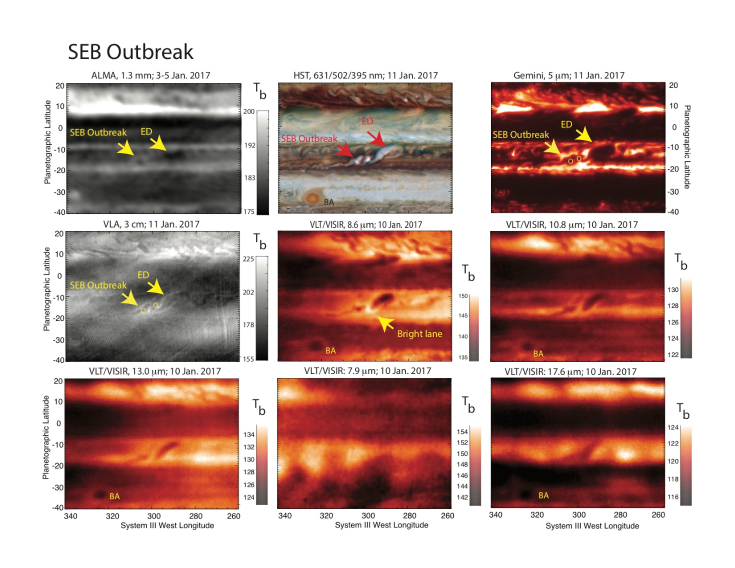
Figure 11: The SEB outbreak as observed at different wavelengths. Each panel is about 80^∘ in longitude and 60^∘ in latitude. The source of the outbreak, as well as the ED (East Disturbance) is indicated in several panels. The various wavelengths are sensitive to different gases and/or aerosols, and hence probe different depths (and hence different temperatures).

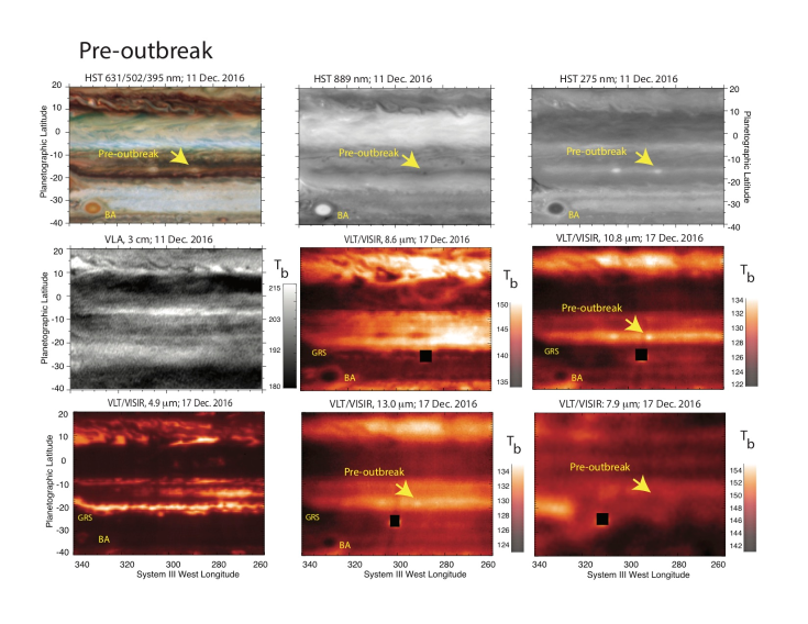
Figure 12: The site of the SEB outbreak in HST and VLA maps (11 Dec. 2016) and at mid-infrared wavelengths (17 Dec. 2016) several weeks before the first plume was seen. The vortex (bright in the visible and mid-IR; dark at 889 nm) where the outbreak took place is indicated by an arrow. The dark square on the mid-IR images blocks out Io, which was visible (saturated) in a background frame.

The pre-outbreak spot is very similar to the one $\sim$20^∘ to the west, except that it displays the small clearing at 889 nm – it is not clear how this difference could predict such a vigorous eruption a few weeks later.

The source of the SEB outbreak (Fig. 11) is dark in the ALMA map, surrounded by a brighter ring, indicative of NH₃ gas rising up to higher (colder) altitudes, with dry gas subsiding around the periphery, like the secondary circulation in small vortices (de Pater et al., 2010). A small brighter lane is visible to the northeast, connecting to a large dark area, referred to as the East Disturbance (ED). The brightness temperature at 1.3 mm of both the source of the SEB outbreak and the ED is consistent with a model of NH₃ gas rising up from the deep atmosphere (Fig. 8).

At mid-IR wavelengths, data taken $\sim$6 days after the ALMA observations, the SEB outbreak and ED are dark at all troposphere-sensing wavelengths (8.6 – 20 $\mu$m), indicative of cold temperatures, enhanced aerosol opacity, or (most likely) a combination of the two (Fig. 11). VLA, HST, and 5-$\mu$m observations were taken one day later. At this time two prominent convective storms are visible on the HST map, with the ED to the northeast. The location of both plumes is indicated on the VLA and 5-$\mu$m maps (yellow circles in the dark areas), both indicative of low brightness temperatures. The ED is also dark on these maps, while bright regions near/around the plume locations and along the ED periphery imply aerosol-free dry subsiding air, so deeper warmer layers are probed. The bright lane at the southwestern edge of the ED in the 8.6-$\mu$m image, sensing a combination of temperature and aerosol opacity at the 500-mbar level, is consistent with this picture. This lane had moved slightly northwards between January 10 and 11, as shown in the Gemini image (Fig. 11); on 10 January, the 5-$\mu$m region coincided in position with the 8.6-$\mu$m lane (not shown). At higher altitudes sensed by the 17.6/18.7/19.5-$\mu$m images, the SEB outbreak and ED are simply cold and embedded in the warmer SEB; due to the lower spatial resolution, details of the structure are washed out. A tail to the south-west of the SEB outbreak is visible in all images, the direction of which is consistent with the gradient in the wind profile. Finally, at 7.9 $\mu$m, probing the stratosphere, a wave with a 20-25 degree longitudinal spacing might be present towards the west of the source outbreak. Such a stratospheric thermal wave was clearly present during the 2010-2011 SEB revival (Fletcher et al., 2017a).

From all maps together, we infer that NH₃ gas is most likely brought up in the convective plume(s), drying out through condensation, and descending along the periphery. Model fits to the plume at the source of the SEB outbreak in the HST data (Section 4.3) corroborate this picture. The cumulative opacity in the SEB plume is about twice that of the background at high altitudes (100–200 mbar), with larger-sized particles, and a quarter of the cumulative opacity between 0.2–0.7 bar (Fig. 9), such as would be expected if particles rise up to much higher altitudes in the plume region. This suggests that the plume consists of particles thrown from lower altitudes high into the atmosphere.

Simultaneously with the Gemini images, we took 5-$\mu$m spectra near the SEB outbreak using NIRSPEC at Keck (Fig. 6). These spectra were taken very close to a bright (hot spot) area, and we have good reasons to believe the data are contaminated by flux from these hot regions. Nevertheless, we can conclude from the in-depth analysis in Section 4.4 that the spectra are consistent with the ED and plume region having thick clouds at the 600-mbar level. Although a best fit to the spectrum suggests no cloud at the 5-bar level, we do not trust this. The gas composition is similar to that of adjacent Hot Spots, with H₂O at 47 ppm at $P>4.5$ bar (as measured with the Galileo Probe; Wong et al., 2004), and zero at higher altitudes. NH₃ line profiles were best matched using 300 ppm at $P>1.2$ bar. With the likely contamination by hot spots, this NH₃ abundance should be taken as a lower limit. Although our ALMA data agree well with this abundance (Fig. 7), due to ALMA’s low spatial resolution this also was taken as a lower limit to the NH₃ abundance.

Fletcher et al. (2017a) compared the convective eruptions triggering the 2010-2011 SEB revival with mesoscale convective storms (MCS) seen on Earth, which show intense precipitation and cold cloud tops (Houze, 1993). As discussed above, the SEB eruptions, like those in the NTB, are probably moist-convective plumes, rising up from the water condensation level. While injection of energy warms the atmosphere relative to its surroundings, resulting in a cyclonic motion, near the top of the plume, where divergence and cooling takes place, an anticyclonic motion is expected (Emanuel, 1994). Since such a motion is in the opposite sense to that expected from the windshear across the SEB, the anticyclones will not persist for long but break up into eddies. Such a sequence of events, starting with a moist-convective plume and ending with its demise, while new plumes arise at the same location (same System-II longitude) was imaged at high spatial resolution by Voyager 1 in Feb. 1979, and modeled by Hueso et al. (2002). The Voyager images closely resemble the present, as well as previous, SEB outbreaks, including the eruption, westward tail, and ED. None of the previous observations, however, yields information below the visible ammonia clouddeck. Our ALMA observations are the first to show that high concentrations of NH₃ gas are brought up in the plume, i.e., the source of the outbreak, as well as in the disturbance to the east. The mid-infrared images show that the top of the plumes are indeed cold, as expected from the models. Hence our data are fully consistent with models of moist convection.

6 Summary

This paper focuses on 1.3- and 3-mm maps constructed from data obtained with ALMA on 3–5 January 2017, just days after the onset of an outbreak in the SEB, and a few months after a reorganization of the NTB. These data are the first to characterize the atmosphere below the cloud layers during/following such outbreaks. Aided also by observations ranging from uv to mid-infrared wavelengths, we have shown that the eruptions are consistent with models where energetic plumes are triggered via moist convection at the base of the water cloud. The plumes bring up ammonia gas from the deep atmosphere to high altitudes, where NH₃ gas is condensing out and the subsequent dry air is descending in neighboring regions. The cloud tops are cold, as shown by mid-infrared data, indicative of an anticyclonic motion, which causes the storm to break up, as expected from similarities to mesoscale convective storms on Earth. The plume particles reach altitudes as high as the tropopause.

Our research shows the importance of simultaneous multi-wavelength observations of transient events, that sense the atmosphere from below the cloud layers to well above the tropopause.

References

Ádámkovics, et al. 2016. Meridional variation in tropospheric methane on Titan observed with AO spectroscopy at Keck and VLT, Icarus, 270, 376-388.

Asay-Davis X.S., Marcus, P.S., Wong, M. H., de Pater, I., 2011. Changes in Jupiter’s Zonal Velocity between 1979 and 2008. Icarus, 211, 1215-1232.

Atkinson, D.H., Pollack, J.B., Seif, A., 1998. The Galileo probe doppler wind experiment: measurement of the deep zonal winds on Jupiter. J. Geophys. Res. 103 (E10), 22911-22928.

Bjoraker, G.L., Wong, M.H., de Pater, I., Hewagama, T., Ádámkovics, M., Orton, G.S., 2018. The Gas Composition and Deep Cloud Structure of Jupiter’s Great Red Spot. Astron. J., 156, #101, 15 pp.

Brown, S., et al., 2018. Prevalent lightning sferics at 600 megahertz near Jupiter’s poles. Nature, 558, 87-90 (DOI: 10.1038/s41586-018-0156-5)

Conrath, B.J., Gierasch, P.J., Leroy, S.S., 1990. Temperature and circulation in the stratosphere of the outer planets. Icarus, 83, 255-281.

de Kleer, K., Luszcz-Cook, S., de Pater, I., Adamkovics, M., Hammel, H., 2015. Clouds and aerosols on Uranus: Radiative transfer modeling of spatially-resolved near-infrared Keck spectra. Icarus, 256, 120-137.

de Pater, I., 1986. Jupiter’s zone-belt structure at radio wavelengths: II. Comparison of observations with model atmosphere calculations, Icarus, 68, 344-365.

de Pater, I., and D.L. Mitchell, 1993, Microwave Observations of the Planets: the Importance of Laboratory Measurements, J. Geophys. Res. Planets, 98, 5471-5490.

de Pater, I., D. Dunn, K. Zahnle and P.N. Romani, 2001. Comparison of Galileo Probe Data with Ground-based Radio Measurements. Icarus, 149, 66-78

de Pater, I., DeBoer, D.R., Marley, M., Freedman, R., Young, R., 2005. Retrieval of water in Jupiter’s deep atmosphere using microwave spectra of its brightness temperature. Icarus, 173, 425-438.

de Pater, I., Wong, M. H., Marcus, P. S., Luszcz-Cook, S., Ádámkovics, M., Conrad, A., Asay-Davis, X., Go, C., 2010. Persistent Rings in and around Jupiter’s Anticyclones - Observations and Theory. Icarus, 210, 742-762.

de Pater, I., Wong, M. H., de Kleer, K., Hammel, H. B., Ádámkovics, M., Conrad, A., 2011. Keck Adaptive Optics Images of Jupiter’s North Polar Cap and Northern Red Oval. Icarus, 213, 559-563.

de Pater, I., Fletcher, L.N., Luszcz-Cook, S.H., DeBoer, D., Butler, B., Hammel, H.B., Sitko, M.L., Orton, G., Marcus, P.S., 2014. Neptune’s Global Circulation deduced from Multi-Wavelength Observations. Icarus, 237, 211-238.

de Pater, I., Sault, R. J., Butler, B., DeBoer, D., Wong, M. H., 2016. Peering through Jupiter’s Clouds with Radio Spectral Imaging, Science, 352, Issue 6290, pp. 1198-1201. (referred to as dP16).

de Pater, I., Sault, R. J., Wong, M. H., Fletcher, L. N., DeBoer, D., Butler, B., 2019. Jupiter’s ammonia distribution derived from VLA maps at 3–37 GHz. Icarus, 322, 168-191. (referred to as dP19)

Dressel, L. Wide Field Camera 3 Instrument Handbook, version 11.0 (STScI, Baltimore MD, 2019).

Emanuel K 1994 Atmospheric Convection (New York: Oxford University Press)

Fletcher, L. N., 2017. Cycles of activity in the Jovian atmosphere. Geophys. Res. Lett. 44, 4725-4729.

Fletcher, L. N., G. S. Orton, P. Yanamandra-Fisher, B. M. Fisher, P. D. Parrish, and P. G. J. Irwin, 2009. Retrievals of atmospheric variables on the gas giants from ground‐based mid‐infrared imaging, Icarus, 200, 154–175, doi:10.1016/j.icarus.2008.11.019.

Fletcher, L.N., G.S. Orton, J.H. Rogers, A. A. Simon-Miller, I. de Pater, M.H. Wong, O. Mousis, P.G.J. Irwin, M. Jacquesson, P.A. Yanamandra-Fisher, 2011. Jovian Temperature and Cloud Variability during the 2009-2010 Fade of the South Equatorial Belt. Icarus, 213, 564-580.

Fletcher, L. N., Greathouse, T. K., Orton, G. S., Sinclair, J. A., Giles, R. S., Irwin, P. G. J., Encrenaz, T., 2016. Mid-infrared mapping of Jupiter’s temperatures, aerosol opacity and chemical distributions with IRTF/TEXES. Icarus, 278, p. 128-161.

Fletcher, L. N., Orton, G. S., Rogers, J. H., Giles, R. S., Payne, A. V., Irwin, P. G. J., Vedovato, M., 2017a. Moist Convection and the 2010-2011 Revival of Jupiter’s South Equatorial Belt. Icarus, 286, 94–117.

Fletcher, L. N., Orton, G. S., Sinclair, J. A., et al., 2017b. Jupiter’s North Equatorial Belt expansion and thermal wave activity ahead of Juno’s arrival, Geophys. Res. Lett., 44, 7140-7148.

Fletcher, L. N., et al., 2018. Jupiter’s Mesoscale Waves Observed at 5 $\mu$m by ground-based observations and Juno JIRAM. Astronomical Journal, 156, 67-80.

Gibson, J., Welch, Wm. J., de Pater, I., 2005. Accurate Jovian Flux Measurements at $\lambda$1cm Show Ammonia to be Sub-saturated in the Upper Atmosphere. Icarus, 173, 439-446.

Hodapp, K. W., et al., 2003. The Gemini Near-Infrared Imager (NIRI). Publ. Astron. Soc. Pac., 115, 814.

Houze, R., 1993. Cloud Dynamics. Vol. 53 of International Geophysics Series. Academic Press.

Hueso, R., Sánchez-Lavega, A., Guillot, T., Oct. 2002. A model for large-scale Moist Convection for the Giant Planets: The Jupiter Case. Icarus 151, 257–274.

Irwin, P. G., Bowles, N., Braude, A. S., Garland, R., & Calcutt, S., 2018. Analysis of gaseous ammonia (NH₃) absorption in the visible spectrum of Jupiter, Icarus, 302, 426-436.

Karim, R. L., deBoer, D., de Pater, I., Keating, G. K., 2018. A Wideband Self-consistent Disk-averaged Spectrum of Jupiter Near 30 GHz and Its Implications for NH₃ Saturation in the Upper Troposphere. Astron. J., 155, article id. 129, 8 pp.

Kataza et al., 2000, COMICS: the cooled mid-infrared camera and spectrometer for the Subaru telescope, Proceedings of Society of Photo-Optical Instrumentation Engineers (SPIE), Vol. 4008, 1144–1152

Kunde, et al., 1996, Cassini infrared Fourier spectroscopic investigation, Proceedings of Society of Photo-Optical Instrumentation Engineers (SPIE), volume 280, 162–177.

Lagage, P. O., et al. (2004), Successful commissioning of VISIR: The mid-infrared VLT instrument, Messenger, 117, 12-16.

Li, C., et al., 2017. The distribution of ammonia on Jupiter from a preliminary inversion of Juno microwave radiometer data. Geophys. Res. Lett., 44, 5317–5325, doi:10.1002/2017L073159.

Lii, P.S., M.H. Wong, and I. de Pater, 2010. Temporal Variation of the Tropospheric Cloud and Haze in the Jovian Equatorial Zone. Icarus, 209, 591-601.

Lindal, G.F., 1992, The atmosphere of Neptune: An analysis of radio occultation data acquired with Voyager 2, Astron. J., 103, 967-982.

Luszcz-Cook, S.H., K. de Kleer, I. de Pater, M. Adamkovics, H.B. Hammel, 2016. Retrieving Neptune’s aerosol properties from Keck OSIRIS observations. I. Dark regions. Icarus, 276, 52-87.

Marcus, P.S., Tollefson, J., Wong, M.H., de Pater, I., 2019. An Equatorial Thermal Wind Equation: Applications to Jupiter. Icarus, 324, 198-223.

McLean, I.S., Becklin, E.E., Bendiksen, O., et al. 1998. Design and development of NIRSPEC: a near- infrared echelle spectrograph for the Keck II telescope. Proc. SPIE 3354, 566-578.

Mizumoto, S., 2017. ‘2016-2017 Mid-SEB Outbreak Final Report’, posted on ALPO-Japan web site: alpo-j.asahikawa-med.ac.jp/kk17/j170923s.htm

Moeckel, C., Janssen, M.J., de Pater, I., 2019. A fresh look at the Jovian radio emission as seen by Cassini-RADAR and implications for the time variability. Icarus, 321, 994-1012.

Molter, E., et al., 2019. Discovery of a bright equatorial storm on Neptune. Icarus, 321, 324-345.

Rogers, J. H., 1995. The Giant Planet Jupiter, 418 pp., Cambridge Univ. Press, Cambridge, U. K.

Rogers, J. H., 2018. Jupiter in 2016-17, Report no.17: ‘Summary of the mid-SEB outbreak’, on the BAA web site: https://www.britastro.org/node/16772

Sánchez-Lavega, et al., 2017. A planetary-scale disturbance in the most intense Jovian atmospheric jet from JunoCam and ground-based observations. Geophysical Res. Lett. 44, 4679-4686.

Sault, R.J., Engel, C., de Pater, I., 2004. Longitude-resolved Imaging of Jupiter at $\lambda=2$ cm. Icarus, 168, 336-343.

Sault, R. J., Teuben, P. J., & Wright, M. C. H. 1995, A Retrospective View of MIRIAD, in ASP Conf. Ser. 77, Astronomical Data Analysis Software and Systems IV, ed. R. A. Shaw, H. E. Payne, & J. J. E. Hayes (San Francisco: ASP), 433-436.

Showman, A.P., de Pater, I., 2005. Dynamical implications of Jupiter’s tropospheric ammonia abundance. Icarus, 174, 192-204.

Sugiyama, K., Nakajima, K., Odaka, M., Kuramoto, K., Hayashi, Y.-Y., 2014. Numerical simulations of Jupiter’s moist convection layer: Structure and dynamics in statistically steady states. Icarus, 229, 71-91.

Tollefson, J., Wong, M.H., de Pater, I., Simon, A., Orton, G.S., Rogers, J.H., Atreya, S.K, Cosentino, R.G., Januszewski, W., Morales-Juberias, R., Marcus, P.S., 2017. Changes in Jupiter’s Zonal Wind Profile preceding and during the Juno mission. Icarus, 296, 163-178.

van Dokkum, P. G., 2001. Cosmic-ray rejection by Laplacian edge detection. Publ. Astron. Soc. Pacific, 113, 1420-1427.

Vasavada, A. R., Showman, A. P., 2005. Jovian atmospheric dynamics: an update after Galileo and Cassini. Rep. Prog. Phys. 68, 1935–1996.

Wong, M.H., Mahaffy, P.R., Atreya, S.K., Niemann, H.B., Owen, T.C., 2004. Updated Galileo probe mass spectrometer measurements of carbon, oxygen, nitrogen, and sulfur on Jupiter. Icarus 171, 153-170.

Wong, M.H., 2011. Fringing in the WFC3/UVIS detector. In Proc. 2010 Space Telescope Science Institute Calibration Workshop (eds Deustua, S. & Oliveira, C.) 189-200 (STScI, Baltimore MD, 2011).

Wong, M. H., Atreya, S. K., Kuhn, W. R., Romani, P. N., & Mihalka, K. M. 2015. Fresh clouds: A parameterized updraft method for calculating cloud densities in one-dimensional models. Icarus, 245, 273

Wong, M.H., et al., 2019. High-resolution UV/optical/IR imaging of Jupiter in 2016-2018. In Prep.