A parallel-in-time approach for wave-type PDEs

Abstract

Numerical solutions to wave-type PDEs utilizing method-of-lines require the ODE solver’s stability domain to include a large stretch of the imaginary axis surrounding the origin. We show here that extrapolation based solvers of Gragg-Bulirsch-Stoer (GBS) type can meet this requirement. Extrapolation methods utilize several independent time stepping sequences, making them highly suited for parallel execution. Traditional extrapolation schemes use all time stepping sequences to maximize the method’s order of accuracy. The present method instead maintains a desired order of accuracy while employing additional time stepping sequences to shape the resulting stability domain. We optimize the extrapolation coefficients to maximize the stability domain’s imaginary axis coverage. This yields a family of explicit schemes that approaches maximal time step size for wave propagation problems. On a computer with several cores we achieve both high order and fast time to solution compared with traditional ODE integrators.

1 Introduction

Time integration of ODEs is an inherently sequential process, since each forward step ought to be based on the most recent information available. Three conceivable options for achieving some level of parallel-in-time are (i) to have correction calculations follow the explicit forward steps as closely behind as possible, letting them catch up frequently, (ii) to carry out ‘preparatory’ calculations that are based on trying to anticipate later solution states, and (iii) to exploit extrapolation ideas. While all of these concepts have been pursued for systems of ODEs, as summarized in CMO10 ; KW14 , their performance is unclear for ODE systems arisen from method-of-lines (MOL) discretization of wave-type PDEs. The additional requirement that arises then is that the ODE solver’s stability domain must include a quite large stretch of the imaginary axis surrounding the origin. We show here that extrapolation-based ODE solvers of Gragg-Bulirsch-Stoer (GBS) type can meet this requirement. In particular, one such scheme that we will focus on steps forward explicitly using six cores as fast as Forward Euler (FE) does on one core, but combines eighth order of accuracy with a generously sized stability domain. In contrast to linear multistep methods, it needs no back levels in time to get started. The present approach is compared against explicit Runge-Kutta (RK) methods for a PDE test problem.

Standard Richardson extrapolation schemes utilize a square Vandermonde-type system to compute the extrapolation weights. This system is constructed to cancel successive terms in the asymptotic error expansion of the time stepper. By allowing more columns than rows in the system - that is, more extrapolation components than order constraints - we create an underdetermined system that grants degrees of freedom to optimize the extrapolated stability domain. For wave-type PDEs stepped with method-of-lines we optimize the stability domain along the imaginary axis. We achieve stability domains far larger than those of both the square extrapolation systems and other standard ODE integrators, thereby enabling large time step sizes and thus faster time to solution.

2 GBS-type ODE solvers

2.1 GBS concept

We consider first the problem of advancing forward in time an ODE of the form $y^{\prime}(t)=f(t,y)$, where the unknown function $y(t)$ is either scalar or vector valued. The complete time interval of interest is split into $N$ sections. For each of these sections, the basic (unextrapolated) GBS scheme consists of the steps

$$\left\{{\begin{array}[]{ll}{\displaystyle\frac{y_{1}-y_{0}}{h}}=f(t_{0},y_{0})&\textrm{Forward Euler (FE)}\\ {\displaystyle\frac{y_{n+1}-y_{n-1}}{2h_{\phantom{}}}}=f(t_{n},y_{n})&\textrm{Leap-frog (LF), }n=1,2,\ldots,N\\ y_{N}^{*}=\dfrac{1}{4}(y_{N-1}+2y_{N}+y_{N+1})&\textrm{Averaging},\end{array}}\right.$$ (1)

after which $y_{N}^{*}$ is accepted as the new value at time $t_{N}.$ The initial FE step is accurate to first order, while the subsequent LF steps are second order accurate. One would therefore expect $y_{N}^{*}$ to be accurate to at most second order, and have an error expansion in which all further powers of $h$ would be present. Remarkably, for any smooth (linear or nonlinear) function $f(t,y)$, it transpires that, if $N$ is even, all odd powers in the expansion will vanish BS66 ; G65 ; HNW87 ; L91 :

$$\text{Error}=y_{N}^{*}-y(t_{N})=a_{2}h^{2}+a_{4}h^{4}+a_{6}h^{6}+\ldots$$ (2)

The form of the expansion makes Richardson extrapolation particularly efficient since, each time this is applied, the result will gain two orders of accuracy. For example, the results from four completely independent calculations over the same section in time, using different $h$-values, can be combined to give an $\mathcal{O}(h^{8})$-accurate result. These four calculations require no communications between each other, and can therefore be run simultaneously on separate cores.

Even when not counting the cost of the work on the extra cores, the GBS approach does not offer any striking benefits for standard ODE systems, unless possibly if extrapolated to very high orders. However, in the present context of wave-type PDEs, the situation becomes different, since GBS methods can be designed to feature particularly favorable stability domains.

2.2 Stability domains for GBS-type methods

Appendix A briefly summarizes the definition of an ODE solver’s stability domain, explains its significance in the context of MOL time stepping, and provides stability domain information for some well-known explicit ODE solvers. These domains should be contrasted to the corresponding ones for GBS methods described below. The imaginary stability boundary (ISB) of an ODE solver is defined as the largest value such that the imaginary axis is included from $-i\cdot\text{ISB}$ to $+i\cdot\text{ISB}$. For solvers that lack any imaginary axis coverage, we define their ISB to be zero.

In order to provide a fair comparison between different methods, we will from now on further normalize all ISB values by the number of function evaluations that each step requires and denote this ISB${}_{\text{n}}$. For example, we divide $\textrm{R}\textrm{K}_{4}$’s ISB, stated in Appendix A as 2.8284, by four to compensate for its four stages (with one function evaluation in each), i.e. we list its ISB${}_{\text{n}}$ as 0.7071 $(=1/\sqrt{2}$). Similarly, the ISB${}_{\text{n}}$ for the 13-stage $\textrm{R}\textrm{K}_{8}$ method becomes 0.2848. With this normalization, the largest feasible ISB${}_{\text{n}}$ for any explicit method becomes one JN81 , which is realized by the LF scheme. Since the longest distance a solution can be advanced per function evaluation is proportional to the time stepping method’s ISB${}_{\text{n}}$, a key goal will be to design a method that has both high order and a large ISB${}_{\text{n}}$.

Stability domains and ISBs for GBS-type schemes do not appear to have been studied until in FZL07 . One key observation made there was that GBS schemes of orders 4, 8, 12, … will feature positive ISBs, whereas schemes of order 6, 10, 14, … will not. Hence, in what follows we study only schemes with order divisible by four.

3 Optimizing the Stability Domain

3.1 Introduction to ISB Optimization

Stability domain optimization has been well studied in the literature. The class of steppers that maximizes ISB given stability polynomial order $N+1$ was found independently by Kinnmark and Gray KG84a and Sonneveld and van Leer SL85 . The methods divide a time interval into $N$ evenly spaced steps. A Forward Euler predictor and Backward Euler corrector pair initiates the time step, then $N-1$ leap frogs bring us to the end of the time interval. This class of methods has order of accuracy at most two, and achieves an ISB${}_{\text{n}}=N/(N+1)$.

Kinnmark and Gray demonstrate third and fourth order accurate stability polynomials in KG84b that converge to the optimal ISB as number of subintervals increases. Interestingly, the first two methods of this class are the third order and fourth order explicit Runge-Kutta methods with three and four stages, respectively. Thus RK₄ is optimal in the sense that it fully utilizes its four function evaluations to maximize time step for wave-type problems. It is therefore an excellent candidate for comparison with the optimized schemes that follow.

3.2 GBS Stability Domain Optimization

In Richardson extrapolation schemes one sets up a square Vandermonde system to compute the weights guaranteeing a specified order of accuracy. If we allow the number of components in the extrapolation scheme to increase beyond those necessary for maintaining order of accuracy we obtain an underdetermined system with degrees of freedom. We utilize these degrees of freedom to optimize the stability domain along a contour in the complex plane.

Extrapolation allows us to eliminate successively higher order terms in the asymptotic error expansion of our solution. To do so, for each of $m$ integrators we divide the time interval $H$ into $n_{i}$ steps of size $h_{i}=H/n_{i}$, $i=1,2,\ldots,m$. We then construct a linear system to eliminate terms through order $p-1$ in the error expansion, yielding a $p$-order accurate solution. In the case of GBS integrators, the odd coefficients in the asymptotic expansion are zero. Thus we may drop the constraint equations for odd powers of $h_{i}$, obtaining a system of $\frac{p}{2}$ equations:

$$\underbrace{\addstackgap[16pt]{\begin{bmatrix}1&1&\ldots&1\\ h_{1}^{2}&h_{2}^{2}&\ldots&h_{m}^{2}\\ \vdots&\vdots&\ddots&\vdots\\ h_{1}^{p-2}&h_{2}^{p-2}&\ldots&h_{m}^{p-2}\end{bmatrix}_{\frac{p}{2}\times m}}}_{V}\hskip 2.15277pt\underbrace{\addstackgap[5pt]{\begin{bmatrix}[1]c_{1}\\ c_{2}\\ \\ \vdots\\ \\ c_{m}\end{bmatrix}_{m}}}_{c}=\underbrace{\addstackgap[16pt]{\begin{bmatrix}[1]1\\ 0\\ \vdots\\ 0\end{bmatrix}_{\frac{p}{2}}.}}_{b}$$ (3)

When $m=\frac{p}{2}$ we have a square matrix which corresponds to the usual Richardson extrapolation schemes. The matrix is invertible when $n_{i}\neq n_{j},i\neq j$, and so we solve for the weight vector $c$, which we apply to the individual integrated solutions to form the combined solution at the end of the time interval.

By allowing $m>\frac{p}{2}$ the system becomes underdetermined and we may enforce order constraints while optimizing selected features of the stability domain. The optimization algorithm was adapted from the polynomial optimization formulation in KA12 ; details are provided in Appendix B.

3.3 Fully-Determined Optimization Results

We first investigate optimal step count selection for fully determined extrapolation schemes. For schemes of order $p$ we test each combination of $\frac{p}{2}$ step counts up to a set maximum, here chosen to be 24. Each combination yields a set of uniquely determined extrapolation weights. We then select the combination of step counts that maximizes ISB${}_{\text{n}}$ of the extrapolated stability domain. Tab. 1 contains the tabulated results for orders eight, twelve and sixteen. The schemes all have generous imaginary axis coverage and can be implemented efficiently on three, four and five cores respectively.

Table 1: Optimal step count sequences and ISB${}_{\text{n}}$ for the fully-determined schemes

Order	Cores	Step Counts	ISB${}_{\text{n}}$
8	3	2,16,18,20	0.5799
12	4	2,8,12,14,16,20	0.4515
16	5	2,8,10,12,14,16,18,22	0.4162

3.3.1 Eighth Order

The eighth order, three-core scheme has ISB${}_{\text{n}}=0.5799$ with the following step counts and uniquely determined weights:

$$\begin{matrix}[1.5]\text{Step Counts }\\ \text{Weights }\end{matrix} \begin{matrix}[1.5]:\\ :\end{matrix}\hskip 4.30554pt\begin{matrix}[1.5]2,&16,&18,&20\\ -\frac{1}{498960},&\frac{65536}{9639},&-\frac{531441}{25840},&\frac{250000}{16929}.\end{matrix}$$

3.3.2 Twelfth Order

The twelfth order, four-core scheme has ISB${}_{\text{n}}=0.4515$ with the following step counts and weights:

$$\begin{matrix}[1.5]\text{Step Counts }\\ \text{Weights }\end{matrix} \begin{matrix}[1.5]:\\ :\end{matrix}\hskip 4.30554pt\begin{matrix}[1.5]2,&8,&12,&14,&16,&20\\ -\frac{1}{157172400},&\frac{4096}{155925},&-\frac{59049}{15925},&\frac{282475249}{15752880},&-\frac{4194304}{178605},&\frac{9765625}{954261}.\end{matrix}$$

3.3.3 Sixteenth Order

The sixteenth order, five-core scheme has ISB${}_{\text{n}}=0.4162$ and utilizes the step count sequence $\{2,8,10,12,14,16,18,22\}$. Extrapolation weights can be computed by solving the corresponding Vandermonde system (3). We omit them here since the weights are ratios of large integers in both the numerators and denominators.

3.4 Underdetermined Optimization Results

Using the optimization methodology described in Appendix B we optimize the ISB of GBS-type methods up to order sixteen. Increasing the number of extrapolation components leads to an increase in ISB${}_{\text{n}}$. Since for explicit schemes the maximum ISB${}_{\text{n}}$ is one we expect the relative gains of adding more components to eventually saturate. By evenly distributing work across CPU cores we can demonstrate the relationship between available processors and maximal time step size. This correspondence between core count and ISB${}_{\text{n}}$ is shown in Fig. 1. Here we observe that efficiency saturation occurs around ten cores for all orders of accuracy; the saturation value itself is strongly dependent on the order of accuracy.

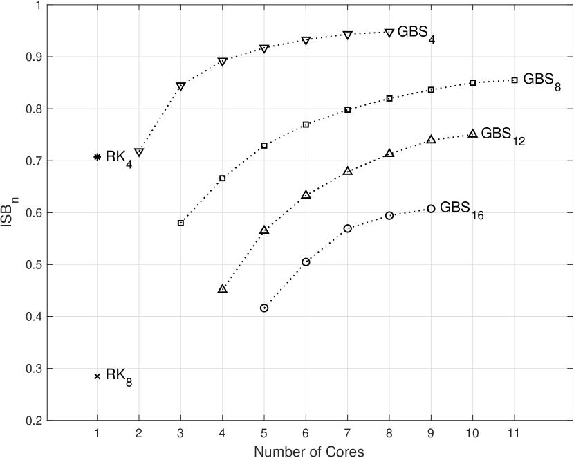
Figure 1: Trends for optimized ISB${}_{\text{n}}$ versus core count for methods of various order

We achieve the best optimization results by utilizing all (even) step counts up to a maximum dependent on the number of available CPU cores. The $m$ extrapolation components then have subinterval counts $\{2,4,\ldots,2m\}$, with $m$ set by the available processing resources. We denote the number of subintervals at which ISB${}_{\text{n}}$ can no longer be increased $N_{\text{opt}}$ and aggregate the results for each order of accuracy in Tab. 2. The stability domains for each core count are plotted in Fig. 2. Results demonstrate a tradeoff between optimal ISB and order of accuracy as is typical of explicit time integrators.

Table 2: Largest optimized ISB${}_{\text{n}}$ obtained for the underdetermined schemes

Order	Cores	$N_{\text{opt}}$	ISB${}_{\text{n}}$
4	8	28	0.9477
8	11	40	0.8551
12	10	36	0.7504
16	9	32	0.6075

The capping of $N_{\text{opt}}$ is an artifact of the optimizer. Our convex solver fails to produce methods with larger ISB if we increase the number of free variables beyond those presented in Tab. 2. We believe that by addressing the conditioning of the Vandermonde system as in KA12 one can continue further along the curves presented in Fig. 1. Extrapolating these curves shows the schemes do not converge to the optimal ISB${}_{\text{n}}=1$; the exact tradeoff between order of accuracy and optimal ISB is a topic of future research.

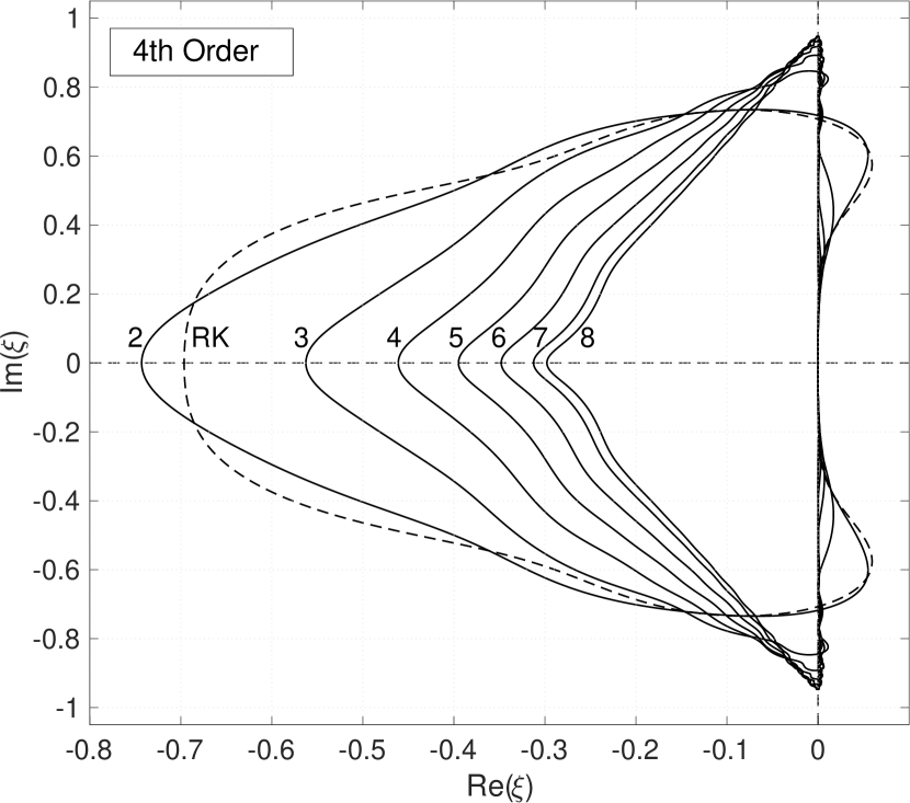
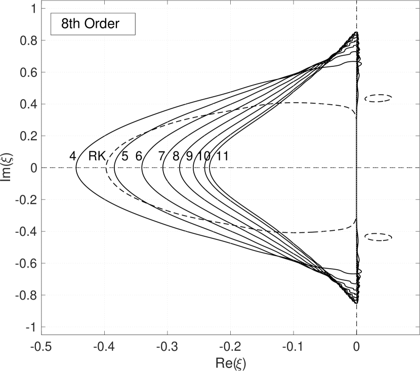
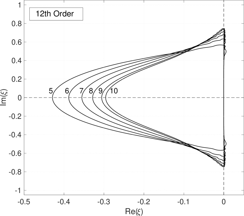
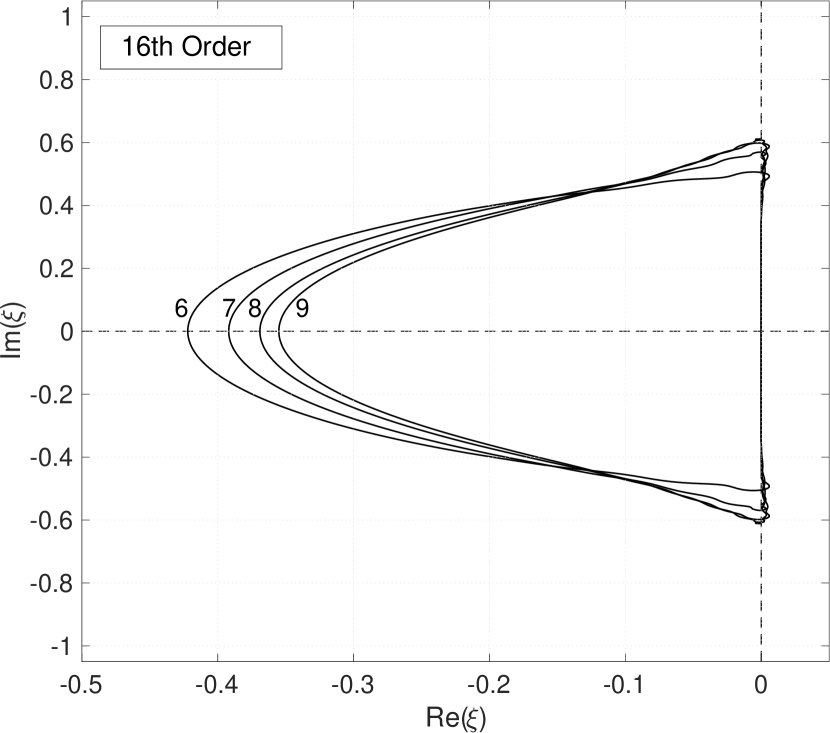
Figure 2: Optimized stability domains labeled with number of cores required to implement the schemes, with fourth and eighth order Runge-Kutta (RK) stability domains for comparison

3.5 Leading Order Error

Let the time integrator’s stability polynomial, as defined in Appendix A, be denoted $R(\xi)$. For a method of order $p$, the stability domain’s boundary follows the imaginary axis surrounding the origin linearly up to deviation on the order $p+1$. To compute the leading error coefficient we set the stability polynomial $R(\xi)=e^{i\theta}$. Taking the complex logarithm of the polynomial and Taylor expanding yields a power series for $\theta(\xi)$. We then compute the inverse series to find $\xi(\theta)=i\theta+a_{p+1}(i\theta)^{p+1}+a_{p+2}(i\theta)^{p+2}+\mathcal{O}\left(\theta^{p+3}\right)$. Since we consider only methods with order divisible by four we simplify as follows:

$$\xi(\theta)=i\theta+ia_{p+1}\theta^{p+1}-a_{p+2}\theta^{p+2}+\mathcal{O}\left(\theta^{p+3}\right).$$ (4)

Departure from the imaginary axis is governed by the $a_{p+2}$ coefficient. We then require $a_{p+2}$ to be negative to ensure the stability domain has a positive ISB. Accuracy is determined by the $a_{p+1}$ coefficient; Fig. 3 presents this coefficient for each method as a function of number of cores.

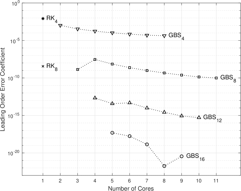
Figure 3: Leading order error term $a_{p+1}$ for the optimized methods

The leading order error coefficient decays toward zero as number of cores increases while holding order fixed. This implies the underdetermined extrapolation schemes do not trade away numerical precision for achieving large ISBs - they instead gain significantly in accuracy.

3.6 Core Partitioning

In order to achieve the theoretical efficiencies presented in Sect. 3.4 we require a work partitioning scheme that distributes the individual time steppers amongst the cores. For a specified maximum subinterval count $N_{\text{max}}$ we achieve the largest ISB${}_{\text{n}}$ by utilizing all even step counts up to $N_{\text{max}}$. For a fixed number of cores, here denoted $n_{\text{cores}}$, we can always evenly distribute the work when we choose $N_{\text{max}}=4\cdot n_{\text{cores}}-2$. This corresponds to folding together onto a single core pairs of integrators with step counts adding to $N_{\text{max}}$. For example, with $N_{\text{max}}=10$, we evenly load three cores with step counts {10, {8, 2}, {6, 4}}.

The GBS scheme requires $N+1$ function evaluations for an integrator with $N$ subintervals. When stacking multiple integrators on a single core we share the first function evaluation since it takes identical arguments for all time steppers. We can in principle share this evaluation among all cores but communication overhead may make this approach less efficient.

3.7 Method Specification

Let the $m\times\frac{p}{2}$-sized Vandermonde matrix in (3) be denoted $V$. When we have $m>\frac{p}{2}$ the system is underdetermined. We then choose $\frac{p}{2}$ dependent step counts to meet the order constraints and collect these into the step count sequence $\{n_{\text{dep}}\}$. The associated extrapolation weight vector is denoted $c_{\text{dep}}$ and the corresponding columns of $V$ denoted $V_{\text{dep}}$. Likewise collect the remaining step counts into the $\left(m-\frac{p}{2}\right)$-length step count sequence $\{n_{\text{free}}\}$ and label corresponding extrapolation weights $c_{\text{free}}$ and Vandermonde columns $V_{\text{free}}$. Then the constraint equations may be written

$$V_{\text{dep}}c_{\text{dep}}+V_{\text{free}}c_{\text{free}}=b.$$ (5)

The Vandermonde system order constraints must be met exactly. We thus omit floating-point coefficients for $c_{\text{dep}}$ in the text; they are best computed symbolically then converted to the desired floating point format. We may readily compute $c_{\text{dep}}$ with the relation

$$c_{\text{dep}}=V_{\text{dep}}^{-1}\left(b-V_{\text{free}}c_{\text{free}}\right),$$ (6)

so one only needs the step count sequences $\{n_{\text{dep}}\}$ and $\{n_{\text{free}}\}$ and weight vector $c_{\text{free}}$ to fully specify a scheme.

3.8 Methods of Choice

In this section we present two eighth order methods and one twelfth order method with rational coefficients for convenient use. In order to provide robustness to spurious discretized eigenvalues sitting slightly in the right-half plane we push the optimization curve into the positive reals. This disturbs the ISB${}_{\text{n}}$ very little and makes the method suitable for local differentiation stencils generated for example by RBF-FD (radial basis function-generated finite difference) approximations FFBook .

To generate the following schemes we first optimize the free coefficients using the optimization methodology described in Appendix B. The optimization contour is chosen to trade off a small amount of imaginary axis coverage for an area containing the positive reals away from the origin. We then perform a search over a set of rational numbers that closely approximate the floating point free coefficients. We select a set with small integers in the numerator and denominator which disturbs the scheme’s stability domain very little. These coefficients are reported below.

3.8.1 The Eighth Order, Six Core Method: GBS_8,6

The following eighth order method achieves a robust stability domain for wave-type PDEs on six cores and is therefore dubbed GBS_8,6. The scheme’s ISB${}_{\text{n}}$ is 0.7675, a 0.26% reduction from the optimal six core value of 0.7695. The scheme can be implemented using the following step counts and extrapolation weights:

$$\{n_{\text{dep}}\} =\hskip 1.29167pt\left\{\begin{matrix}2,&4,&6,&10\end{matrix}\right\}$$

$$\begin{matrix}[1.5]\{n_{\text{free}}\}\\ \vphantom{\bigg{[}}c_{\text{free}}\end{matrix} \begin{matrix}[1.5]=\\ \vphantom{\bigg{[}}=\end{matrix}\hskip 4.30554pt\begin{matrix}[1.5]\{&8,&12,&14,&16,&18,&20,&22&\}\hphantom{{}^{T}.}\\ \bigg{[}&\frac{2165}{767488},&\frac{13805}{611712},&\frac{4553}{72080},&\frac{14503}{66520},&\frac{27058}{7627},&-\frac{86504}{5761},&\frac{40916}{3367}&\bigg{]}^{T}.\end{matrix}$$

The dependent weights can be computed exactly by inverting the corresponding Vandermonde system. The scheme’s stability domain is plotted in Fig. 4, with a zoom-in around the imaginary axis on the right-hand side.

This method can be run efficiently on six cores with time steps 6.25 times larger than those of RK₄. After normalizing for number of function evaluations, the scheme achieves time-to-solution $0.7675/0.7071=8.5\%$ faster than RK₄ but with eighth order of accuracy. Compared to RK₈, though, we achieve time-to-solution 269% faster. As will be seen in Sect. 4.1, speed-up to achieve a specified accuracy is far improved over RK₄ due to the size of the leading order error term combined with eighth order convergence to the true solution.

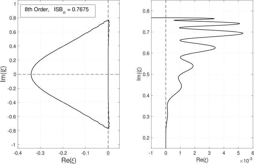
Figure 4: Stability domain of the eighth order, six core scheme (left), and zoom (right)

3.8.2 The Eighth Order, Eight Core Method: GBS_8,8

Likewise for the six core method, we produce a robust stability domain for an eighth order scheme that runs efficiently on eight cores, called GBS_8,8. The scheme’s ISB${}_{\text{n}}$ is 0.8176, a 0.24% reduction from the optimal eight core value, 0.8196. The scheme utilizes the following step counts and extrapolation weights:

$$\{n_{\text{dep}}\} =\hskip 1.29167pt\left\{\begin{matrix}2,&26,&28,&30\end{matrix}\right\}$$

$$\{n_{\text{free}}\} =\hskip 1.29167pt\left\{\begin{matrix}4,&6,&8,&10,&12,&14,&16,&18,&20,&22\end{matrix}\right\}$$

$$c_{\text{free}} =\begin{matrix}[1.5]\bigg{[}&\frac{6833}{476577792},&\frac{10847}{91078656},&\frac{15235}{34643968},&\frac{383}{321152},&\frac{543}{198784},&\ldots\end{matrix}$$

$$\hskip 68.88867pt\begin{matrix}[1.5]\ldots&\frac{9947}{1741056},&\frac{6243}{543104},&\frac{6875}{296192},&\frac{1401}{28496},&\frac{17713}{152688},&\frac{6375}{19264}&\bigg{]}^{T}.\end{matrix}$$

The scheme’s stability domain is plotted in Fig. 5, with a zoom-in around the imaginary axis on the right-hand side.

This method can be run efficiently on eight cores with time steps 8.96 times larger than those of RK₄. After normalizing for number of function evaluations the scheme achieves time-to-solution 15.6% faster than RK₄, and 287% faster than RK₈. The two additional cores grant us a 6.5% increase in efficiency over GBS_8,6.

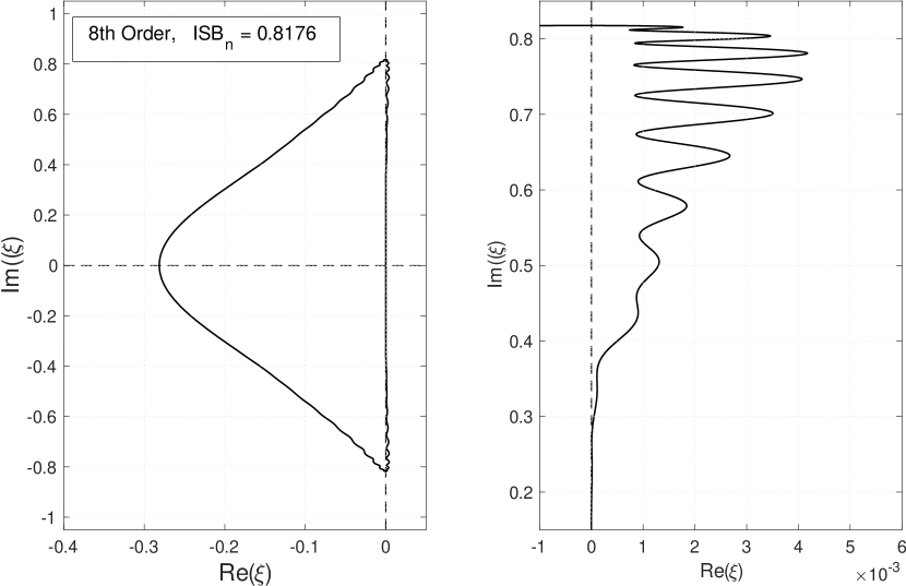
Figure 5: Stability domain of the eighth order, eight core scheme (left), and zoom (right)

3.8.3 The Twelfth Order, Eight Core Method: GBS_12,8

The following twelfth order method runs on eight cores and is therefore dubbed GBS_12,8. The scheme’s ISB${}_{\text{n}}$ is 0.7116, a 0.17% reduction from the optimal eight core value of 0.7128. The scheme can be implemented using the following step counts and extrapolation weights:

$$\{n_{\text{dep}}\} =\hskip 1.29167pt\left\{\begin{matrix}2,&8,&10,&16,&24,&26\end{matrix}\right\}$$

$$\{n_{\text{free}}\} =\hskip 1.29167pt\left\{\begin{matrix}4,&6,&12,&14,&18,&20,&22,&28,&30\end{matrix}\right\}$$

$$c_{\text{free}} =\begin{matrix}[1.5]\bigg{[}&\frac{235}{21030240256},&\frac{4147}{1612709888},&\frac{11521}{39731200},&\frac{2375}{3528704},&\frac{6435}{708736},&\ldots\end{matrix}$$

$$\hskip 116.24963pt\begin{matrix}[1.5]\ldots&\frac{1291}{15780},&\frac{11311}{4672},&-\frac{180864}{751},&\frac{222080}{2079}&\bigg{]}^{T}.\end{matrix}$$

Stable time steps with GBS_12,8 are 7.79 times larger than those of RK₄ and, after normalization, time-to-solution is improved by 0.6%. This (very) modest efficiency improvement is drastically offset by the twelfth order of convergence of the method - wall time to achieve a desired accuracy is far shorter than that of RK₄.

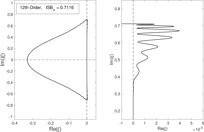
Figure 6: Stability domain of the twelfth order, eight core scheme (left), and zoom (right)

4 Numerical Results

The following results demonstrate the optimized time steppers on a test problem with known analytic solutions.

4.1 One-Way Wave Equation

To demonstrate the performance benefit over standard time steppers from the literature we run the periodic one-way wave equation,

$$\tfrac{\partial}{\partial t}u(x,t)+\tfrac{\partial}{\partial x}u(x,t)=0,\hskip 17.22217pt 0\leq x\leq 1,\hskip 8.61108ptt>0,$$ (7)

$$u(x,0)=\tfrac{1}{2}\left(1-\cos{2\pi x}\right), 0\leq x\leq 1,$$

utilizing the rational-coefficient GBS_8,6 and GBS_12,8 methods, with RK₄ as reference. Spatial derivatives are spectral to ensure errors are due to the time stepping algorithm alone. We run all time steppers near their respective limits of stability, at $\lambda=\Delta t/\Delta x=\frac{.99}{\pi}\times\text{ISB}$, where the factor of $\pi$ arises from the spectral spatial derivatives. After convecting the wave once around the periodic interval we compute the absolute error with respect to the analytic solution, then refine in both time and space.

Convergence to the analytic solution for the various methods is demonstrated in Fig. 7. For fair comparison across methods, the horizontal axis is time step normalized by the number of function evaluations per step. Thus vertical slices correspond to equal time-to-solution, neglecting the overhead of sharing data across cores. We use a high precision floating point library MCT15 for computation since machine precision is achieved in the high order methods before we can establish a trendline. Coefficient truncation to double precision causes error to stagnate at $10^{-14}$ and $10^{-12}$ for the eighth and twelfth order methods, respectively. To obtain full floating point precision to $10^{-16}$ the extrapolation coefficients must be precise to twenty significant digits.

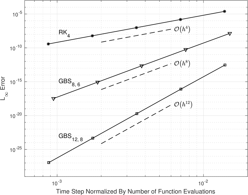
Figure 7: Convection error vs. normalized time step for various methods

5 Conclusions

We have presented a scheme for maximizing the time step size for extrapolation based ODE solvers. To do so we construct an underdetermined Vandermonde system, then optimize the weights to maximize the stability domain along a given curve in the complex plane. For wave-type PDEs we utilize GBS integrators and optimize the methods for imaginary axis coverage. We achieve large ISB values for methods through order sixteen which, when implemented on a computer with several cores, yield faster time to solution than standard Runge-Kutta integrators.

The optimization method leaves both the time integrator and desired contour of stability as user parameters. Changing the ODE integrator in turn changes the stability polynomial basis, which immediately affects the resulting extrapolated stability domains. The GBS integrator maintains large ISB through extrapolation; other integrators may be better suited for different desired stability domains. Future work therefore involves identifying other suitable integrators for stability domain optimization in different contexts.

The underdetermined extrapolation scheme saturates in parallelism around ten cores. We can improve scalability by incorporating the optimized schemes as local building blocks in time-parallel solvers like Parareal LMT01 . These solvers are known to be less efficient with wave-type PDEs G15 . Stable algorithms may be achieved by optimizing the global time-parallel integrators rather than optimizing the coarse and fine grid propagators individually. These degrees of freedom provide more flexibility than optimizing only the local schemes and is a promising research direction for improving time to solution for wave-type equations.

Appendix Appendix A Stability domains and imaginary axis coverage for some standard classes of ODE solvers

A.1 Stability domains and their significance for MOL time stepping

Each numerical ODE integration technique has an associated stability domain, defined as the region in a complex $\xi$-plane, with $\xi=h\lambda$, for which the ODE method does not have any growing solutions when it is applied to the constant coefficient ODE

$$y^{\prime}=\lambda y\>.$$ (8)

For a one-step method the stability polynomial, here denoted $R(\xi)$, is the numerical solution after one step for Dahlquist’s test equation (8) NW91 . The method’s stability domain is then

$$S=\{\xi\in\mathbb{C}:|R(\xi)|\leq 1\}.$$ (9)

When solving ODEs, the stability domain can provide a guide to the largest time step $h$ that is possible without a decaying solution being misrepresented as a growing one. In the context of MOL-based approximations to a PDE of the form $\frac{\partial u}{\partial t}=L(x,t,u)$, the role of the stability domain becomes quite different, providing necessary and sufficient conditions for numerical stability under spatial and temporal refinement: all eigenvalues to the discretization of the PDE’s spatial operator $L$ must fall within the solver’s stability domain. For wave-type PDEs, the eigenvalues of $L$ will predominantly fall up and down the imaginary axis. As long as the time step $h$ is small enough, this condition can be met for solvers that feature a positive ISB, but never for solvers with ISB = 0.

A.2 Runge-Kutta methods

All $p$-stage RK methods of order $p$ feature the same stability domains when $p=1,2,3,4.$ For higher orders of accuracy, more than $p$ stages (function evaluations) are required to obtain order $p$. The $\textrm{R}\textrm{K}_{4}$ scheme used here is the classical one, and the $\textrm{R}\textrm{K}_{8}$ scheme is the one with 13 stages, introduced by Prince and Dormand PD81 , also given in HNW87 Table 6.4. Their normalized stability domains are shown in Fig. 8. Their ISBs are 2.8284 and 3.7023, respectively.

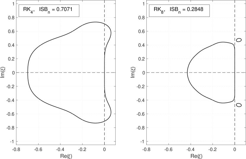
Figure 8: Normalized stability domains for RK₄ (left) and RK₈ (right)

Appendix Appendix B ISB Optimization Algorithm

B.1 Optimization Formulation

Let the extrapolated GBS stability polynomial be denoted $R(\xi)$, and the individual stability polynomials from each of $m$ extrapolation components be denoted $P_{i}(\xi)$. Then we have

$$R(\xi)=\sum_{i=1}^{m}{c_{i}P_{i}(\xi)}$$ (10)

for extrapolation weights $c_{i}$, $1\leq i\leq m$. We collect the monomial coefficients of each $P_{i}(\xi)$ into the rows of a matrix, denoted $P(\xi)$. Then $R(\xi)$ can be more compactly expressed as $R(\xi)=c^{T}P(\xi)$. Now let the left-hand-side Vandermonde matrix from (3) be denoted $V$, and the right-hand-side constraint vector be denoted $b$. Then our order constraint equation (3) can be rewritten as $Vc=b$.

Denoting the time step size $h$, and given a curve $\Lambda\subset\mathbb{C}$, we specify the optimization problem as follows:

$$\underset{c_{1},c_{2},\ldots,c_{m}}{\text{maximize}} h$$ (11)

subject to $$|R(h\lambda)|-1\leq 0,\;\forall\lambda\in\Lambda.$$

$$Vc=b$$

Following the work of Ketcheson and Ahmadia in KA12 , we reformulate the optimization problem in terms of an iteration over a convex subproblem. Minimizing the maximum value of $|R(h\lambda)|-1$ over the weights $c_{i}$ is a convex problem (see KA12 ). We therefore define the subproblem as follows:

$$\underset{c_{1},c_{2},\ldots,c_{m}}{\text{minimize}} \max_{\lambda\in\Lambda}{(|R(h\lambda)|-1)}$$ (12)

subject to $$Vc=b$$

Calling the minimax solution to (12) $r(h,\Lambda)$, we can now reformulate the optimization problem as:

$$\underset{c_{1},c_{2},\ldots,c_{m}}{\text{maximize}} h$$ (13)

subject to $$r(h,\Lambda)\leq 0$$

The optimization routine was implemented with the CVX toolbox for MATLAB CVX14 using a bisection over time step $h$. Results presented in this paper use the software OPTISB AE19 to optimize the stability domains.

B.2 Comparison to Optimizing Monomial Coefficients

The main theoretical difference between our current algorithm and the algorithm presented in KA12 is the basis over which coefficients are optimized. In KA12 the authors optimize directly the coefficients to the stability polynomial in the monomial basis. This yields an optimal stability polynomial that must be approximated with a Runge-Kutta integrator. The polynomial is therefore fed into a second optimization routine to compute the Runge-Kutta coefficients.

In the extrapolation coefficient optimization we operate directly on linear combinations of the time stepper stability polynomials. The true optimal stability polynomial therefore may not be in the space of extrapolated GBS time stepper stability polynomials. However, the resulting stability polynomial is immediately realizable and we require no further optimization stage to generate our time stepping algorithm.

B.3 Implementing Order Constraints

To guarantee accuracy we require order constraints to be satisfied to machine precision. Most optimization routines accept equality constraints that will hold within a certain tolerance. Due to ill-conditioning of the Vandermonde systems we prefer to explicitly enforce the order constraints in the convex optimization. As in Sect. 3.7 we split the stability polynomials into two groups which take on the “dep” and “free” subscripts, denoting dependent and optimized quantities, respectively. The dependent weights guarantee the extrapolation scheme achieves the specified order of accuracy. The remaining weights are our optimization variables. Thus the stability polynomial is computed as follows:

$$R(\xi)=c_{\text{dep}}^{T}P_{\text{dep}}(\xi)+c_{\text{free}}^{T}P_{\text{free}}(\xi).$$ (14)

Order constraints take the form (5) which yields the dependent weight computation (6). Splitting the weights apart reduces the number of design variables and, in practice, leads to better solutions than when utilizing equality constraints.

References

- (1) Advanpix LLC.: Multiprecision Computing Toolbox for MATLAB. Version 4.6.4.13322 (2019). URL http://www.advanpix.com/
- (2) Bulirsch, R., Stoer, J.: Numerical treatment of ordinary differential equations by extrapolation methods. Numer. Math. 8, 1–13 (1966)
- (3) Christlieb, A.J., MacDonald, C.B., Ong, B.W.: Parallel high-order integrators. SIAM J. Sci. Comput. 32, 818–835 (2010)
- (4) Ellison, A.C.: OPTISB: Stability Domain Optimization for Extrapolated GBS Integrators (2019). URL https://github.com/acellison/optisb
- (5) Fornberg, B., Flyer, N.: A Primer on Radial Basis Functions with Applications to the Geosciences. SIAM, Philadelphia (2015)
- (6) Fornberg, B., Zuev, J., Lee, J.: Stability and accuracy of time-extrapolated ADI-FDTD methods for solving wave equations. J. Comp. Appl. Math. 200, 178–192 (2007)
- (7) Gander, M.J.: 50 Years of Time Parallel Time Integration. In: T. Carraro, M. Geiger, S. Körkel, R. Rannacher (eds.) Multiple Shooting and Time Domain Decomposition Methods, pp. 69–113. Springer International Publishing (2015)
- (8) Gragg, W.B.: On extrapolation algorithms for ordinary initial value problems. SIAM J.Numer. Anal. 2, 384–404 (1965)
- (9) Grant, M., Boyd, S.: CVX: Matlab Software for Disciplined Convex Programming. Version 2.1 (2018). URL http://cvxr.com/cvx
- (10) Hairer, E., Nørsett, S.P., Wanner, G.: Solving Ordinary Differential Equations I - Nonstiff Problems. Springer Verlag, Berlin (1987)
- (11) Hairer, E., Wanner, G.: Solving Ordinary Differential Equations II - Stiff and Differential-Algebraic Problems, 2 edn. Springer Verlag, Berlin (1996)
- (12) Jeltsch, R., Nevanlinna, O.: Stability of explicit time discretizations for solving initial value problems. Numer. Math. 37, 61–91 (1981)
- (13) Ketcheson, D.I., Ahmadia, A.J.: Optimal stability polynomials for numerical integration of initial value problems. Communications in Applied Mathematics and Computational Science 7, 247–271 (2012)
- (14) Ketcheson, D.I., bin Waheed, U.: A comparison of high-order explicit Runge-Kutta, extrapolation, and deferred correction methods in serial and parallel. Comm. App. Math.and Comp. Sci. 9, 175–200 (2014)
- (15) Kinnmark, I.P.E., Gray, W.G.: One step integration methods of third-fourth order accuracy with large hyperbolic stability limits. Mathematics and Computers in Simulation XXVI, 181–188 (1984)
- (16) Kinnmark, I.P.E., Gray, W.G.: One step integration methods with maximum stability regions. Mathematics and Computers in Simulation XXVI, 87–92 (1984)
- (17) Lambert, J.D.: Numerical Methods for Ordinary Differential Systems: The Initial Value Problem. Wiley, New York (1991)
- (18) Lions, J.L., Maday, Y., Turinici, G.: Résolution d’EDP par un schéma en temps “pararéel”. Comptes Rendus de l’Académie des Sciences - Series I - Mathematics 332(7), 661–668 (2001)
- (19) Prince, P.J., Dormand, J.R.: High order embedded Runge-Kutta formulae. J. Comp. Appl. Math. 7, 67–75 (1981)
- (20) Sonneveld, P., van Leer, B.: A minimax problem along the imaginary axis. Nieuw Archief voor Wiskunde 3 (4), 19–22 (1985)