Testing the Robustness of Robust Phase Estimation

Abstract

The Robust Phase Estimation (RPE) protocol was designed to be an efficient and robust way to calibrate quantum operations. The robustness of RPE refers to its ability to estimate a single parameter, usually gate amplitude, even when other parameters are poorly calibrated or when the gate experiences significant errors. Here we demonstrate the robustness of RPE to errors that affect initialization, measurement, and gates. In each case, the error threshold at which RPE begins to fail matches quantitatively with theoretical bounds. We conclude that RPE is an effective and reliable tool for calibration of one-qubit rotations and that it is particularly useful for automated calibration routines and sensor tasks.

I Introduction

The standard, circuit model of quantum computation requires discrete, unitary operations (gates). However, physical implementation of these gates is not naturally discrete. For one-qubit gates it is useful to picture a unitary operation as a specific rotation of the Bloch sphere, with an axis and an angle of rotation that can be parametrized by three real numbers. Careful calibration of these parameters is necessary in order to compute accurately using the gate Wright et al. (2019); Erhard et al. (2019); Kelly et al. (2018).

When a single unitary operation is concatenated into a sequence of several identical operations, the resulting angle of rotation is linear in the number gates. Measurements of the quantum state after such a sequence can cause small changes in the angle of the individual gate to appear quadratically as changes in the resulting projection probabilities. As a result, the error of a computation can scale as the square both of the angular error on each operation and of the number of operations. Because of this scaling, small errors in calibrating operation rotation angles using simple calibration experiments can still lead to significant error in the context of longer gate sequences.

In its original form, the Robust Phase Estimation (RPE) protocol was proposed as a practical method for estimating the axis and angle of a single qubit rotation. The protocol was originally developed by Kimmel et al. (2015) and tested in experiments by Rudinger et al. (2017). The robustness of RPE refers to its ability to estimate these two parameters even when other parameters of the experiment are poorly calibrated or prone to stochastic errors. In this paper we describe three separate experiments that demonstrate the robustness of RPE to injected errors chosen to represent common experimental error sources.

The RPE protocol consists of performing gate sequences of several different lengths; in each sequence the same gate is repeated, so that the final rotation angle compounds linearly. The gate sequences themselves are very similar to the standard “Rabi flopping” procedure, in which the rotation interaction is applied continuously for varying durations before qubit measurement. The result of Rabi flopping is ideally a sinusoidal dependence of final state population on interaction duration, from which one can extract a “Rabi frequency” that can in turn be used to calculate the rotation angle realized in any finite duration. The primary differences between Rabi flopping and RPE are that RPE repeats an operation with a fixed duration, instead of continuously varying the duration of a single operation, and that the structure and analysis procedure of RPE are more complex.

In this work, we focus only on using RPE to estimate the angle of the rotation, called $\theta$ in this work, and not on estimating the rotation axis (called $\theta$ in the original formulation). From a practical standpoint, RPE can determine the rotation angle of a fixed gate duration much more efficiently than Rabi flopping, where efficiency is measured by the number of gate applications required to achieve a given precision in the estimation of the angle.

RPE succeeds or fails in a binary fashion; the estimate it produces is either correct (within a pre-determined confidence region) or it is incorrect, sometimes by a large angle. The protocol can fail at each sequence length (independently) due to shot noise or to errors in the implementation of the quantum operations. When each sequence is repeated sufficiently many times to remove shot noise concerns and the operation errors are small enough, the protocol always succeeds in producing an estimate of the rotation angle within its guaranteed confidence region. The robustness of RPE is defined by this feature that the protocol reliably succeeds even when these errors are significant.

Rabi flopping experiments are useful for diagnostic experiments, where protocol efficiency is less important and an experimenter can identify and process unexpected results. In contrast, the robustness and efficiency of RPE make it ideal for automated calibration of quantum systems or for automated sensor experiments where there is no human oversight. Gate set tomography (GST) is another useful calibration protocol for diagnosing quantum computing experiments. Where the RPE protocol attempts to estimate one or two parameters of a gate while ignoring imperfections in others, GST attempts to fully characterize all parameters of the gate. Ref. Rudinger et al. (2017) clearly examines the differences in cost and utility for the two protocols and finds that RPE is significantly more efficient for single parameter calibrations.

The remainder of this paper is organized as follows. In Section II, we summarize our implementation of the RPE protocol. Our experimental apparatus is described in Section III. In Section IV, we describe the errors against which we test the robustness of RPE. The results of these tests follow in Section V. Finally, we comment in Section VI on the wide range of parameter estimation experiments which could benefit from RPE.

II RPE Protocol

In this section, we provide a practical description of the RPE protocol as applied in our experiments. Consider calibrating the rotation angle $\theta$ of a qubit operation described by

$$Y_{\theta}=\cos(\theta/2)\mathbb{I}-i\sin(\theta/2)\sigma_{Y}$$ (1)

where $\mathbb{I}$ is the identity matrix and $\sigma_{Y}$ is the Pauli $Y$-matrix.

We perform two sets of experiments, where the operation of interest is repeated $\{n\}$ times for various values of $n$, and the sets are differentiated by the initial qubit state. The experiments all terminate with a single, projective measurement. We repeat each experiment $M_{n}$ times (subsequently referred to as “samples”) and record the number of times we observe the +1 eigenstate. The observed number of the +1 results for the two sets of experiments are denoted by $x_{n}$ and $y_{n}$, and their values in the limit of large $M_{n}$ can be predicted using the following formulas:

$$x_{n}=M_{n}\left|\braket{1}{Y_{\theta}^{n}}{0}\right|^{2}\qquad y_{n}=M_{n}\left|\braket{1}{Y_{\theta}^{n}}{+}\right|^{2},$$ (2)

where the state $\ket{+}$ is equal to $(\ket{0}+\ket{1})/\sqrt{2}$ and $\{\ket{0},\ket{1}\}$ are the $Z$-eigenstates of the qubit. In our experiment we always initially prepare $\ket{0}$. The state $\ket{+}=Y_{\pi/2}\ket{0}$ is generated from the initial state with a $Y_{\pi/2}$ operation.

In order to account for non-idealities in the experiments, we follow the convention of Ref. Kimmel et al. (2015) and write the expected probability of observing the +1 eigenstate in the experiments corresponding to $x_{n}$ and $y_{n}$ as

$$p_{x}(n) = \frac{1-\cos(n\theta)}{2}\pm\delta_{x}(n)$$

$$p_{y}(n) = \frac{1+\sin(n\theta)}{2}\pm\delta_{y}(n),$$ (3)

where we have introduced additive error terms $\delta_{x,y}$ which may be $n$-dependent. When the $\delta_{x,y}$ terms are zero, we can estimate the total rotation $n\theta$, modulo $2\pi$, by noting that

$$\tan(n\theta)=\frac{2p_{y}(n)-1}{1-2p_{x}(n)},$$ (4)

and using $x_{n}/M_{n}$ and $y_{n}/M_{n}$ as estimates of $p_{x,y}(n)$ gives

$$n\theta=\tan^{-1}\left(\frac{y_{n}-M_{n}/2}{M_{n}/2-x_{n}}\right),$$ (5)

We note that the inability to discriminate $n\theta=0$ from $2\pi$ can typically be remedied in practice, by repeating the protocol with a gate using the same physics but a smaller intended angle.

When the error terms $\delta_{x,y}$ are non-zero, our estimate of $n\theta$ can be biased. Additionally, if we collect too few samples, shot noise, which is proportional to $1/\sqrt{M_{n}}$, can lead to erroneous results. These considerations are described in great depth in Ref. Kimmel et al. (2015).

The RPE protocol achieves high efficiency by specifying that only certain values of $n$ (gate repetitions) need to be performed, namely $n=2^{j-1}$ where $j\in\{1,2,3,\ldots,L\}$ and $L$ is chosen as a function of the desired precision of the estimate. The $j$th measurement restricts the estimate of $\theta$:

$$\theta-\theta_{\mathrm{actual}}\in\left(-\frac{\pi}{2^{j}},\frac{\pi}{2^{j}}\right].$$ (6)

Each successive doubling of the repetition number cuts the range of the angle estimate bound in half. The supplemental information to Rudinger et al. (2017) provides pseudocode for determining $\theta$ including enforcement of the range restriction from preceding steps. Ref. Kimmel et al. (2015) also provides the projected probability of protocol success conditioned only on statistical errors. Here success is defined to be an application of the protocol in which the true value of $\theta$ lies within the bounds output by the protocol. With the range restriction provided in Eq. (6), Kimmel et al. proved in Kimmel et al. (2015) that RPE is robust in the presence of errors and will succeed provided the total additive error is bounded by $|\delta_{x,y}(n)|<\delta_{\mathrm{bound}}\equiv 1/\sqrt{8}$ for all repetitions $\{n\}$.

In practice, it is likely to be difficult to estimate the additive error a priori. For example, without knowing the angle of the gate under inspection, the experimenter will not know the expected final state of the length $n$ sequence and cannot estimate the impact of asymmetric measurement errors. Even more difficult is the case of gate errors associated with colored noise, where the apparent error magnitude scales non-linearly with the number of gates in the sequence. Errors that are mutually uncorrelated, such as measurement errors or errors due to decay events, are simpler to bound as a function of sequence length, and we focus on them in this manuscript.

It is important to note that as additive error increases, more samples are required for RPE to succeed, and the required $M_{n}$ diverges at the $1/\sqrt{8}$ bound, as described in Kimmel et al. (2015). A prescription for choosing $M_{n}$ as a function of the predicted additive error and sequence length is provided therein. Furthermore, because each sequence length constrains the next estimate of $\theta$, the probability that RPE fails is the sum of the probability of failing at each step.

In this paper, we demonstrate experimentally that, for three error sources that are expected to behave additively, the RPE protocol is as robust as promised. This is evaluated by observing the failure rate of RPE for the gate $Y_{\pi/2}$ as a function of injected (artificially introduced) error sources.

III Experimental System

All experiments described herein are performed on a single ${}^{171}\mathrm{Yb}^{+}$ ion trapped above a GTRI-Honeywell BGA trap Guise et al. (2015). The relevant portion of the atomic energy level diagram is shown in Figure 1a. Doppler cooling, state preparation, and state detection are all performed with the same 369 nm beam through electro-optic modulation, similar to Olmschenk et al. (2007). This beam is switched on and off with an acousto-optic modulator (AOM). The qubit states are chosen from the ground-state hyperfine manifold (Figure 1b) to be $\ket{0}\equiv\ket{F=0,m_{F}=0}$ and $\ket{1}\equiv\ket{F=1,m_{F}=0}$. We label the auxiliary states $\ket{\pm 1}\equiv\ket{F=1,m_{F}=\pm 1}$.

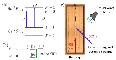
Figure 1: (a) ${}^{171}\mathrm{Yb}^{+}$ energy level diagram. The required 369 nm laser transitions are shown for Doppler cooling (C), initial state preparation (SP), and detection (D). (b) State labels in ${}^{2}S_{1/2}$ hyperfine manifold. The qubit levels are $\ket{0}$ and $\ket{1}$. (c) System overview. Laser beam geometry and microwave horn for qubit operations are overlaid on an image of the trap chip.

One-qubit rotations are driven with microwaves emitted from a horn outside the vacuum chamber as depicted in Figure 1c. We control the frequency, amplitude, and phase of the microwave drive by mixing an approximately 200 MHz DDS signal with a local oscillator at $12.442\,812$ GHz. The upper sideband of this mixing is resonant with the transition from $\ket{0}$ to $\ket{1}$. The mixer output is amplified to a maximum of approximately 1.6 W, high enough to achieve a minimum $\pi/2$-rotation time of $T_{\pi/2}\approx 4~{}\mu$s. However, for all the reported RPE measurements, we reduce the amplitude and use $T_{\pi/2}=10$ to 30 $\mu$s to reduce amplitude errors caused by the thermal duty cycle of the microwave amplifier chain.

While RPE can be used to calibrate any rotation, we choose $Y_{\pi/2}$ (i.e. $\theta=\pi/2$ in Eq. (1)) for our base gate. This means that we prepare $\ket{+}=(\ket{0}+\ket{1})/\sqrt{2}$ with the same gate we repeat for the RPE sequence. Prior to each measurement set, we use an RPE sequence with no intentionally injected errors to calibrate the $\pi/2$ operation for a fixed $T_{\pi/2}$ by adjusting the microwave amplitude. With a maximum sequence length of $2^{7}$ gates and 128 repetitions of each sequence, RPE bounds the calibration at $\pm\pi/2^{8}$, or a fractional uncertainty of 0.8%. In practice, however, we observe much lower statistical uncertainty, similar to the behavior observed in Rudinger et al. (2017), and repeated calibration produces the same microwave amplitude to within 0.04%. Following the full set of RPE trials for each type of error, we repeat the amplitude calibration and find that it is consistent to within 0.2%.

We initially calibrate the microwave frequency to within 1 Hz of the qubit resonance and find that the qubit frequency drifted less than 2 Hz after each data set. The gate error associated with this slow frequency drift is $\approx 10^{-8}$ per gate; compared with the $\approx 10^{-6}$ per gate error associated with drifting amplitude, this error is inconsequential. With these stable, well-calibrated gates, we inject known errors with a significantly larger magnitude as described in the next section.

IV Injecting additive errors

IV.1 Measurement error

We inject error in the measurement process by intentionally misinterpreting the results of our detection operation. The detection consists of counting photons scattered from the ion over a specified duration. When the ion is measured in the $\ket{1}$ state (bright), we collect on average 19 photons during the 400 us detection interval, and when the ion is measured in the $\ket{0}$ state (dark), we collect 0.1 photons. The experimental dark and bright measurement histograms (Figure 2) are nearly Poissonian, except for mixing of the two Poissonians caused by errors in preparation and by the low end tail observed in bright detection events due to off resonant scattering of the detection light Noek et al. (2013). The measurement error associated with these histograms (before error injection) is 1.2%.

To distinguish which state is present after a measurement, we define a threshold for the number of detected photons. If the detected number of photons is less than the chosen threshold, we infer that the ion was in the $\ket{0}$ state; otherwise we infer that it was in the $\ket{1}$ state. The optimal threshold in our experiment was two photons. By intentionally choosing a suboptimal threshold, we introduced an error source in post-processing that is easy to quantify.

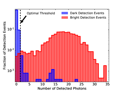
Figure 2: Relative distribution of observed photon counts for putative $\ket{0}$ (dark) and $\ket{1}$ (bright) states. Each experiment is repeated 2500 times. The dashed line shows the optimal detection threshold of 2 photons. Larger detection errors are introduced by choosing a different threshold. At the optimal threshold, the measurement error is 1.2% (sum of the left-most two red bars).

In order to convert from a choice of threshold to an additive error estimate $\delta_{\mathrm{meas}}$, we must identify the maximum error over all possible sequence outcomes. From the measured reference histograms, we calculate the probability that the chosen threshold mis-identifies an observed photon count as bright (when the ion was dark) or dark (when the ion was bright). For a general sequence, we do not know which of the results to expect, so we take the maximum of these probabilities as our pessimistic estimate of $\delta_{\mathrm{meas}}$.

IV.2 Preparation error

The preparation of the $\ket{0}$ state is a stochastic process. The initial state after cooling is a mixture of ${}^{2}S_{1/2}$ manifold states. During preparation, the population in the $\ket{0}$ state exponentially approaches some limiting value close to one within a time $\approx 2~{}\mu$s as depicted in Figure 3. In order to artificially introduce preparation errors, we simply limit the preparation time.

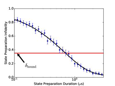
Figure 3: State preparation error as a function of operation duration. We typically use a 50 $\mu$s optical pumping duration to ensure high fidelity initialization in $\ket{0}$; intentionally using a shorter duration injects error. Over the plotted range, the exponential fit to the infidelity $E$ as a function of initialization duration $t$ is $E(t)=0.95e^{-1.5t}+0.025$. At short duration, the infidelity limit is due to asymmetric state populations after Doppler cooling. At long duration, the apparent initialization infidelity is limited by measurement error. The $1/\sqrt{8}$ limit for additive error in RPE corresponds to a preparation time of about 700 ns.

At the laser frequency used for preparation, 369 nm light excites the ${}^{2}S_{1/2},F=1$ to ${}^{2}P_{1/2},F^{\prime}=1$ transitions (see Figure 1a). From the $F^{\prime}=1$ states, the ion may decay into any of the ${}^{2}S_{1/2}$ manifold states. Repetition of this scattering process depletes population from the ${}^{2}S_{1/2},F=1$ manifold. With our beam polarization, we expect the rates of scatter from the $\ket{\pm 1}$ states to be symmetric and faster than the scatter from the $\ket{1}$ state. Because the $\ket{\pm 1}$ states are unaffected by the gates of the RPE sequence, population in these states after initialization is always measured in the bright state and may or may not appear as an error, depending on the ideal result of the sequence. In the worst case, this population sums with the population in the $\ket{1}$ state to constitute the additive error of initialization.

In this worst case, the probability of initialization error after a preparation interval $t$ is equal to the population in the $F=1$ manifold after that interval. Figure 3 shows this population as a function of the preparation time $t$ in our diagnostic experiment. We use this result to convert between $t$ and $\delta_{\mathrm{prep}}$. For example, we observe that a preparation time of about 700 ns corresponds to the theoretical $\delta=1/\sqrt{8}$ threshold for RPE success. Because this comparison represents a worst case error, the RPE protocol is expected to tolerate even shorter preparation times in some instances.

IV.3 Phase damping error

In order to investigate an additive error that scales with the length of the gate sequence, we illuminate the ion during the entire sequence with dim 369 nm light tuned to the ${}^{2}S_{1/2},F=1\rightarrow{}^{2}P_{1/2},F^{\prime}=0$ transition. A 369 nm photon scattering off the ion causes it to excite and spontaneously decay if and only if the ion is in the $F=1$ manifold (including the $\ket{1}$ state). Because we rotated the polarization of the 369 nm light to excite $\sigma^{+}/\sigma^{-}$ transitions preferentially, any population that decayed to the $\ket{\pm 1}$ states was quickly re-excited and transferred to the $\ket{1}$ state. The effect of this aggregate process, considered as an error, is to dephase the qubit: it does not lead to population mixing of the $\ket{0}$ or $\ket{1}$ states, but it does lead to decay of superpositions of those states. Nielsen and Chuang refer to this as phase damping Nielsen and Chuang (2010); an example of controllably inducing a dephasing/phase damping channel is given by Urrego et al. (2018). The decay events we introduce through this scattering process occur discretely and independently, so we expect the aggregate error probability they induce to approach one as a simple exponential in time.

We control the intensity of the 369 nm light addressing the ion by changing the RF power applied to an AOM. Calibrating the absolute magnitude of the phase damping errors is challenging because we do not have a direct measurement of the rate of photon scatter by the ion. To the extent that the AOM responds proportionally to RF power, however, we can estimate the relative scattering rates at different AOM settings. In the course of performing RPE experiments with a known rotation angle, we can also directly observe the additive error we introduce in each sequence by comparing results with and without the injected errors.

Because the phase damping error only affects superpositions of $\ket{0}$ and $\ket{1}$ states, its effective instantaneous strength changes over the course of each RPE sequence as the superposition state changes. As long as the characteristic time scale of the error is longer than the $\pi$-time of the applied rotations and many rotations are applied, it is possible to average this effect out and treat the error as if it has a constant effective strength.

We note as an aside that this approximation breaks down, and the error behavior changes notably, when the 369 nm intensity is high and the inverse scattering rate is faster than the gate time. In this case, the possibility of excitation and decay constantly project the state and the unitary gates are suppressed. This limit was evident in experiments performed with large injected errors, although it is not relevant for the results presented in the next section.

V Results

For all experiments testing the robustness of RPE to injected error, we used a maximum sequence length of $2^{7}$ calibrated $Y_{\pi/2}$ gates and a constant number of samples ($M_{n}$) independent of the sequence length. For each trial of the RPE protocol, we computed the RPE estimate $\theta_{\mathrm{est}}$ of the gate angle using the pseudocode in the supplemental information to Rudinger et al. (2017). For each value of injected error, we conducted between 25 and 100 trials of the RPE protocol. The rate of failure, based on Eq. (6), is defined as the fraction of experiments where $\left|\theta_{\mathrm{est}}-\pi/2\right|>\pi/2^{8}$.

V.1 Detection

A common error source in experimental trapped-ion measurements comes from drift in the intensity of the detection light at the ion, due for example to positional drift of the beam. This drift changes the photon scattering rate and leads to a different optimal threshold as described in Section IV.1. In order to mimic this error and test RPE, we intentionally degrade the measurement operation in RPE by changing the detection threshold used in post-processing. Each RPE sequence used $M_{n}=32$ samples, and the observed rate of failure for 100 trials is shown in Figure 4. RPE succeeds in accurately estimating the gate angle despite large measurement error. As expected (see Eq. (V.16) in Kimmel et al. (2015)), we observe a steep transition between success and failure near the theoretical bound of $\delta_{\mathrm{meas}}\approx 1/\sqrt{8}$.

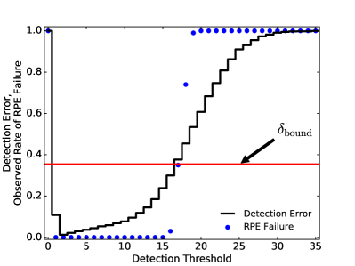
Figure 4: Observed RPE failure rate as a function of the detection threshold (circles). The solid black curve shows the maximum detection error probability, $\delta_{\mathrm{meas}}$, defined in Section IV.1 and computed from the histograms in Figure 2. We observe a sharp onset of RPE failure when the threshold is set at 17 counts, in good agreement with when $\delta_{\mathrm{meas}}>\delta_{\mathrm{bound}}$. Similarly, RPE also fails when enough dark detections are mislabeled as bright, a situation which only occurs for a threshold of zero.

V.2 Initialization

We intentionally degrade the fidelity of our state preparation by shortening its duration, with consequences described in Section IV.2. While preparation is not frequently a large source of error in quantum applications, it can become one when the preparation involves entangled states, such as for recent clock and sensor experiments Ruster et al. (2017); Ockeloen et al. (2013). We chose to explore the combined effects both of injecting error and of changing the number of samples ($M_{n}$) used in the protocol.

In Figure 5, we show the rate of RPE success for $\delta_{\mathrm{prep}}$ between 0.54 (0.40 $\mu$s) and 0.24 (0.99 $\mu$s). For the center row of Figure 5, we performed $M_{n}=32$ samples of each RPE sequence, and we observe agreement between the onset of failure and the $1/\sqrt{8}$ bound based on our estimate of additive error. The number of samples required to reliably achieve a correct estimate increases with the injected error, as indicated by the prescription for $M_{n}$ given by Eq. (V.17) in Kimmel et al. (2015). For $M_{n}<32$, RPE fails frequently even with injected error below the bound due to increased measurement shot noise.

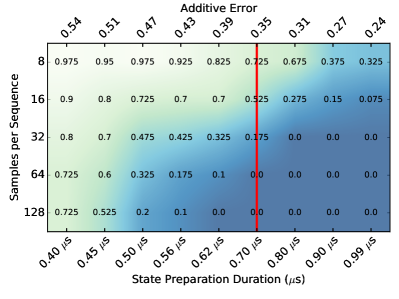
Figure 5: Observed RPE failure rate as a function of qubit preparation duration (bottom axis) and number of samples (left axis). The background shading also indicates the observed failure rate. The top axis shows the maximum additive error $\delta_{\mathrm{prep}}$ corresponding to the qubit preparation duration. We estimate that $\delta_{\mathrm{prep}}$ exceeds $\delta_{\mathrm{bound}}=1/\sqrt{8}$ beyond 700 ns (vertical red line). The boundary of the onset of failure shifts as a function of the number of samples as expected.

V.3 Gate Error: Phase Damping

Spontaneous decay and phase damping bound the coherence time of quantum computations. These processes will bound the maximum sequence length that can be used in the RPE protocol before the additive error exceeds its bound. In order to observe this effect, we intentionally induce phase damping by allowing 369 nm (measurement) light to leak into our experiment, with its intensity reduced by $\{-20,-23,-26,-100\}$ dB from our measurement settings. This process is described in greater depth in Section IV.3.

In Figure 6 we compare the histograms of RPE estimates for these four levels of laser intensity. Because the intensities are well below saturation, we expect spontaneous scattering to be proportional to intensity. Although assigning an absolute phase damping error rate is difficult in our experiment, we observe the same qualitative behavior for RPE failure as is observed for other error sources: the onset of RPE failure is abrupt, and RPE succeeds over a wide range of injected phase damping errors rates.

In contrast to the detection and initialization errors described previously, the total additive spontaneous emission error for a given gate sequence grows with sequence length. Depending on the type of error, some sequence lengths within the RPE protocol can be more likely to cause the RPE estimate to fail. We observed that for the strongest scattering laser intensity tested (-20 dB), the RPE estimate of the rotation angle only exceeded the bound of Eq. (6) at the longest sequence length leading to a clustering of failure events within twice the claimed range of the true value. In the tests with injected preparation or measurement errors, failures were equally likely for any sequence length, resulting in a flatter error distribution.

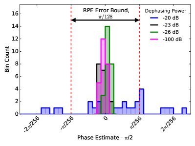
Figure 6: Histograms of rotation angle estimates from RPE with and without additional phase damping errors. The bounds for protocol success are shown as vertical dashed lines. We injected 369 nm (measurement) light at four intensities to drive phase damping. RPE only fails at the strongest intensity (-20 dB), although even here the majority of trials succeed. At lower intensities, we observe that the distribution of estimates is significantly tighter than the provable bounds reported by the protocol.

VI Conclusions

We have shown experimentally that the RPE protocol is robust to errors which occur during state preparation, measurement, and gates, in good agreement with the additive error bound of $1/\sqrt{8}$. Our results are promising for noisy or initially uncalibrated experiments, where the efficiency and robustness of RPE makes it an effective tool for automated gate calibrations.

In order to apply RPE efficiently and successfully, we find that it is important to take into account the dependence of the success probability on the number of samples ($M_{n}$). A greater number of samples becomes more important when the additive error is high, so, in order to maximize efficiency, it is useful to bound the expected error.

Similarly, we observe that the failure of RPE changes in nature depending on whether the error is constant or depends on the sequence length. When initialization and detection errors are larger than gate errors, failures in the RPE protocol can result in estimates that are very far from the true value. In a quantum computing context, this could lead to rare events of mis-calibration causing gates with poor behavior to persist until a new calibration. This catastrophic behavior needs to be treated differently with respect to fault tolerance than typical small-angle coherent errors.

We expect that RPE can also find use within the quantum sensor community. RPE could allow a user to operate a sensor in a poorly controlled environment and with poor initialization and detection operations, as long as the interaction of interest can be repeated reliably. Furthermore, the robustness of RPE to poorly calibrated operations makes it particularly appealing for automated initial calibration of sensors. The main caveat for sensor applications appears to be the need to prepare two orthogonal initial states, although RPE can tolerate significant errors in this operation. In practice, this requirement would be similar to the often-used technique of preparing alternating states for clock measurements Brewer et al. (2019).

Extensions of RPE to non-static parameters and to two-qubit gates are possible directions for future research. Ion temperature and laser intensity variations are just two examples of time-varying parameters. Depending on the root cause, the rotation angle of a gate may change reliably as a function of sequence length or instead may drift randomly; it should be possible to modify RPE to address or mitigate both of these possibilities.

An extension of RPE that calibrates two-qubit gate angle seems straightforward. One simple and necessary adjustment is to rework RPE to account for measurements from two qubits. However, the full calibration of two-qubit gates typically involves more control parameters, so an important challenge is to describe a routine based on RPE that is capable of calibrating all these parameters together both efficiently and robustly.