Abstract

Although distributed computing can significantly reduce the training time of deep neural networks, scaling the training process while maintaining high efficiency and final accuracy is challenging. Distributed asynchronous training enjoys near-linear speedup, but asynchrony causes gradient staleness - the main difficulty in scaling stochastic gradient descent to large clusters. Momentum, which is often used to accelerate convergence and escape local minima, exacerbates the gradient staleness, thereby hindering convergence. We propose DANA: a novel technique for asynchronous distributed SGD with momentum that mitigates gradient staleness by computing the gradient on an estimated future position of the model’s parameters. Thereby, we show for the first time that momentum can be fully incorporated in asynchronous training with almost no ramifications to final accuracy. Our evaluation on the CIFAR and ImageNet datasets shows that DANA outperforms existing methods, in both final accuracy and convergence speed while scaling up to a total batch size of $16$K on $64$ asynchronous workers.

1 Introduction

Modern deep neural networks are comprised of millions of parameters, which require massive amounts of data and long training time (Silver et al., 2016; Raffel et al., 2019). The steady growth of neural networks over the years has made it impractical to train them from scratch on a single worker (computational device). Distributing the computations over several workers can drastically reduce the training time (Dean et al., 2012; Cho et al., 2019; Lerer et al., 2019). Unfortunately, stochastic gradient descent (SGD), which is typically used to train these networks, is an inherently sequential algorithm. Thus, it is difficult to train deep neural networks on multiple workers, especially when trying to maintain fast convergence and high final test accuracy (Keskar et al., 2016; Goyal et al., 2017; You et al., 2020).

Synchronous SGD (SSGD) is a straightforward method to distribute the training process across multiple workers: each worker computes the gradient over its own separate mini-batches, which are then aggregated to update a single model. Because SSGD relies on synchronizations to coordinate the workers, its progress is limited by the slowest worker.

Asynchronous SGD (ASGD) addresses the drawbacks of SSGD by eliminating synchronization between the workers, allowing it to scale almost linearly. However, eliminating the synchronizations induces gradient staleness: gradients were computed on parameters that are older than the parameter server’s current parameters. Gradient staleness is one of the main difficulties in scaling ASGD, since it worsens as the number of workers grows (Zhang et al., 2016). Due to gradient staleness, ASGD suffers from slow convergence and reduced final accuracy (Chen et al., 2016; Cui et al., 2016; Ben-Nun & Hoefler, 2019). In fact, ASGD might not converge at all if the number of workers is too large.

Momentum (Polyak, 1964) has been demonstrated to accelerate SGD convergence and reduce oscillation (Sutskever et al., 2013). Momentum is crucial for high accuracy and is typically used for training deep neural networks (He et al., 2016; Zagoruyko & Komodakis, 2016). However, when paired with ASGD, momentum exacerbates the gradient staleness (Mitliagkas et al., 2016; Dai et al., 2019), to the point that it diverges when trained on large clusters.

Our contribution: We propose DANA: a novel technique for asynchronous distributed SGD with momentum. By adapting Nesterov’s Accelerated Gradient to a distributed setting, DANA computes the gradient on an estimated future position of the model’s parameters, thereby mitigating the gradient staleness. As a result, DANA efficiently scales to large clusters, despite using momentum, while maintaining high accuracy and fast convergence. We show for the first time that momentum can be fully incorporated in asynchronous training with almost no ramifications to final accuracy. We evaluate DANA in simulations as well as in two real-world settings: private dedicated compute clusters and cloud data-centers. DANA consistently outperformed other ASGD methods, in both final accuracy and convergence speed while scaling up to a total batch size of $16$K on $64$ asynchronous workers.

2 Background

The goal of SGD is to find the global minimum of $J(\theta)$ where $J$ is the objective function (i.e., loss) and the vector $\theta\in R^{k}$ is the model’s parameters from dimensional $k$. $x_{t}$ denotes the value of some variable $x$ at iteration $t$. $\xi\in\Xi$ denotes a random variable from $\Xi$, the indices of the entire set of training samples $\Xi=\{1,\cdots,M\}$. $J(\theta;\xi)$ is the stochastic loss function with respect to the training sample indexed by $\xi$. The SGD iterative update rule is the following:

$$\begin{split}g_{t}=\nabla J(\theta_{t};\xi)\quad;\quad\theta_{t+1}=\theta_{t}-\eta g_{t}\end{split}$$ (1)

Where $\eta$ is the learning rate. We also denote $\nabla J(\theta)$ as the full-batch gradient at point $\theta$: $\nabla J(\theta)=\frac{1}{M}\sum_{i=1}^{M}\nabla J(\theta;i)$.

Momentum

Polyak (1964) proposed momentum, which has been demonstrated to accelerate SGD convergence and reduce oscillation (Sutskever et al., 2013). Momentum can be described as a heavy ball that rolls downhill while accumulating speed on its way towards the minima. The gathered inertia accelerates and smoothes the descent, which helps dampen oscillations and overcome narrow valleys, small humps and local minima (Goh, 2017). Mathematically, the momentum update rule (without dampening) is simply an exponentially-weighted moving average of gradients that adds a fraction of the previous momentum vector $v_{t-1}$ to the current momentum vector $v_{t}$.

$$\begin{split}g_{t}=\nabla J(\theta_{t};\xi)\quad&;\quad v_{t}=\gamma v_{t-1}+g_{t}\\ \theta_{t+1}&=\theta_{t}-\eta v_{t}\end{split}$$ (2)

The momentum coefficient $\gamma$ in Equation 2 controls the portion of the past gradients that is added to the current momentum vector $v_{t}$. When successive gradients have a similar direction, momentum results in larger steps (higher speed), yielding up to quadratic speedup in the convergence rate for SGD (Loizou & Richtárik, 2017b; a).

Nesterov

In the analogy of the heavy ball rolling downhill, a higher speed may cause the heavy ball to overshoot the bottom of the valley (the minima), if it does not slow down in time. Nesterov (1983) proposed Nesterov’s Accelerated Gradient (NAG), which allows the ball to slow down in advance. NAG approximates $\hat{\theta}_{t}$, the future value of $\theta_{t}$, based on the previous momentum vector $v_{t}$:

$$\begin{split}\hat{\theta}_{t}=\theta_{t}-\eta\gamma v_{t-1}\quad;&\quad g_{t}=\nabla J(\hat{\theta}_{t};\xi)\\ v_{t}=\gamma v_{t-1}+g_{t}\quad;&\quad\theta_{t+1}=\theta_{t}-\eta v_{t}\end{split}$$ (3)

NAG computes the gradient using the parameters’ estimated future value $\hat{\theta}$ instead of their current value $\theta$. Thus, NAG slows the heavy ball down near the minima so it doesn’t overshoot the goal and climb back up the hill. We refer to this attribute as look-ahead, since it allows peeking at the future position of $\theta$. The gradient $g_{t}$ is computed based on the approximated future parameters $\hat{\theta}_{t}$ and applied to the original parameters $\theta_{t}$ via $v_{t}$.

$$\begin{split}\theta_{t+1}-\hat{\theta}_{t}&=\theta_{t}-\eta v_{t+1}-\theta_{t}+\eta\gamma v_{t}\\ &=\eta\gamma v_{t}-\eta(\gamma v_{t}+g_{t})=-\eta g_{t}\end{split}$$ (4)

Equation 4 shows that the difference between the updated parameters $\theta_{t+1}$ and the approximated future position $\hat{\theta}_{t}$ is only affected by the newly computed gradient $g_{t}$, and not by $v_{t}$. Therefore, NAG can accurately compute the gradient even when the momentum vector $v_{t}$ is large.

3 Gradient Staleness

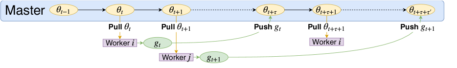
Figure 1: Gradient staleness in the ASGD training process, adapted from Zheng et al. (2017). Gradient $g_{t}$ is stale, since it is computed from parameters $\theta_{t}$ but applied to $\theta_{t+\tau}$.

In this work we consider the common implementation of distributed ASGD that uses a parameter server (also referred to as master), which is commonly used in large-scale distributed settings (Li et al., 2014; Peng et al., 2019; Jayarajan et al., 2019; Hashemi et al., 2019; Zhao et al., 2020). Figure 1 illustrates the ASGD training process and the origin of gradient staleness (Recht et al., 2011). In ASGD training, each worker pulls the up-to-date parameters $\theta_{t}$ from the master and computes a gradient of a single sample (Algorithm 1). Once the computations finish, the worker sends the gradient $g_{t}$ to the master. The master (Algorithm 2) then applies the gradient $g_{t}$ to its current set of parameters $\theta_{t+\tau}$, where $\tau$ is the lag. The variable $x$ for worker $i$ is denoted as $x^{i}$ (for the master, $i=0$). The lag $\tau$ of gradient $g_{t}^{i}$ is defined as the number of updates the master received from other workers while worker $i$ was computing $g_{t}^{i}$.

Algorithm 1 ASGD: worker

  Receive parameters $\theta_{t}$ from master

  Compute gradient $g_{t}\leftarrow\nabla J(\theta_{t};\xi)$

  Send $g_{t}$ to master at iteration $t+\tau$

Algorithm 2 ASGD: master

  Receive gradient $g_{t}$ from worker $i$ (at iteration $t+\tau$)

  Update master’s weights $\theta_{t+\tau+1}\leftarrow\theta_{t+\tau}-\eta g_{t}$

  Send parameters $\theta_{t+\tau+1}$ to worker $i$

In other words, gradient $g_{t}^{i}$ is stale if it was computed on parameters $\theta_{t}$ but applied to $\theta_{t+\tau}$. This gradient staleness is a major obstacle when scaling ASGD: the lag $\tau$ increases as the number of workers $N$ grows (Zhang et al., 2016), decreasing gradient accuracy and ultimately reducing the accuracy of the trained model. As a result, ASGD suffers from slow convergence and reduced final accuracy. In fact, ASGD may not converge at all if the number of workers is too large (Chen et al., 2016; Cui et al., 2016).

From Lag to Gap

Previous works analyze ASGD staleness using the lag $\tau$ (Zhang et al., 2016; Dai et al., 2019). We argue that $\tau$ fails to accurately reflect the effects of the staleness. Instead, we measure the gradient staleness with the recently introduced gap (Barkai et al., 2020). We denote $\Delta_{t+\tau}=\theta_{t+\tau}-\theta_{t}$ as the difference between the master and worker parameters, and define the gap as:

$$\operatorname{G}(\Delta_{t+\tau})=\operatorname{RMSE}(\Delta_{t+\tau})=\frac{\|\Delta_{t+\tau}\|_{2}}{\sqrt{k}}$$

Where $k$ is the number of parameters. When $\Delta_{t+\tau}=0$, the gradient is computed on the same parameters to which it will be applied. This is the case for sequential and synchronous methods such as SGD and SSGD. However, in asynchronous algorithms more workers result in an increased lag $\tau$ and thus a larger gap. Figure 2(a) illustrates that in ASGD adding more worker increases the gap.

Next, we show that the gap is directly correlated with gradient accuracy. A common assumption is that the gradient of $J$ is an L-Lipschitz continuous function:

$$\lVert\nabla J\left(x\right)-\nabla J\left(y\right)\rVert_{2}\leq L\lVert x-y\rVert_{2}\quad,x,y\in\mathbb{R}^{k}$$ (5)

Setting $x=\theta_{t+\tau},y=\theta_{t}$ into Equation 5, we get that the inaccuracy of the stale gradient (with respect to the gradient on $\theta_{t+\tau}$) is bounded by the gap:

$$\begin{split}\lVert\nabla J\left(\theta_{t+\tau}\right)-\nabla J\left(\theta_{t}\right)\rVert_{2}&\leq L\lVert\theta_{t+\tau}-\theta_{t}\rVert_{2}\\ &=L\cdot\sqrt{k}\cdot\operatorname{G}(\Delta_{t+\tau})\end{split}$$ (6)

Equation 6 shows that a smaller gap implies that the stale gradient is more accurate. Conversely, a larger gap means a larger upper bound on the inaccuracy of the stale gradient. The advantage of measuring the staleness using the gap instead of the lag can be illustrated by a simple extreme example of a worker with a lag of $\tau=2$ at time step $t+\tau$. If the two previous updates are in exactly opposite directions and are of the same magnitude, the worker will compute the gradient on the same parameters as the master $\theta_{t+\tau}=\theta_{t}$. Therefore, the gradient will be accurately computed $\nabla J\left(\theta_{t+\tau}\right)=\nabla J\left(\theta_{t}\right)$, as if the lag were zero. However, the lag remains the same ($\tau=2$), while the gap adjusts according to the two updates and is indeed equal to zero.

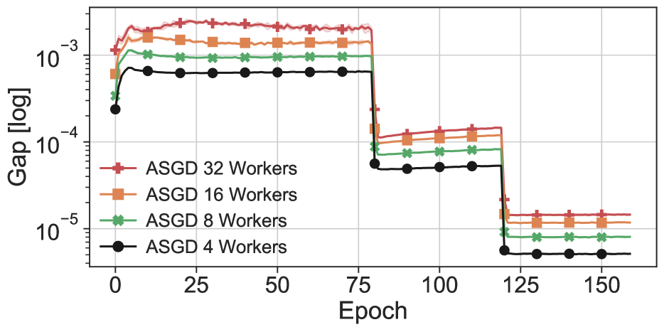
(a) Comparison of the number of workers.

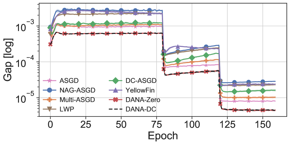
(b) Algorithm comparison (all with 8 workers).

Figure 2: The gap between $\theta_{t+\tau}$ and $\theta_{t}$ while training ResNet-20 on the CIFAR-10 dataset with 2(a) different numbers of workers, and 2(b) different asynchronous algorithms. all algorithms share the same worker update schedules and therefore have an identical lag. Adding workers or using momentum increases the effect of the lag $\tau$ on the gap. The large drops in the gap are caused by learning rate decay. The gap drops at the exact same rate at which the learning rate decays, which empirically shows that the gap correlates linearly with the learning rate $\eta$. The details for the different algorithms are explained in Section 5.

The Effect of Momentum

While momentum and NAG improve the convergence rate and accuracy of SGD, they make it more difficult to scale to additional asynchronous workers. To simplify the analysis, we henceforth assume that all workers have equal computation power. This assumption can be relieved by monitoring the rate of each worker’s updates and weighting them accordingly. We denote by $prev(i,t)$ the last iteration in which worker $i$ sent a gradient to the master before time $t$. For ASGD and NAG-ASGD, $\operatorname{\mathbb{E}}\left[\Delta_{t+\tau}\right]$ is the sum of the gradients and the sum of the momentum vectors, respectively:

$$\operatorname{\mathbb{E}}[\Delta^{\text{ASGD}}_{t+\tau}] =-\eta\sum_{i=1}^{N}g^{i}_{prev(i,t+\tau)}$$ (7)

$$\operatorname{\mathbb{E}}[\Delta^{\text{NAG-ASGD}}_{t+\tau}] =-\eta\sum_{i=1}^{N}v_{prev(i,t+\tau)}$$ (8)

Figure 2(b) demonstrates empirically that the gap of NAG-ASGD is considerably larger than that of ASGD due to momentum, even though the lag $\tau$ in both algorithms is exactly the same.

3.1 Parameter Prediction

The gap arises from the fact that we can not access the future parameters $\theta_{t+\tau}$. Kosson et al. (2020) proposed Linear Weight Prediction (LWP) to estimate future parameters:

$$\theta_{t+\tau}\approx\hat{\theta}^{\text{LWP}}_{t}\triangleq\theta^{0}_{t}-\tau\eta v_{t-1}$$ (9)

To reduce the gap, LWP approximate the master’s future parameters $\theta_{t+\tau}$ in $\tau$ update steps. In other words, LWP scales the NAG estimation according to the number of times $v_{t-1}$ is used throughout the next $\tau$ updates. The worker then computes its gradient on $\hat{\theta}^{\text{LWP}}_{t}$ instead of $\theta^{0}_{t}$. LWP is frequently used in asynchronous model parallel pipelines (Guan et al., 2019; Chen et al., 2018; Narayanan et al., 2019) to reduce the staleness in the backpropagation; during the forward pass LWP estimates the parameters of the backwards pass. Algorithm 3 describes the LWP master algorithm.

Algorithm 3 LWP: master

  Receive gradient $g^{i}$ from worker $i$

  Update momentum $v\leftarrow\gamma v+g^{i}$

  Update master’s weights $\theta^{0}\leftarrow\theta^{0}-\eta v$

  Send estimate $\hat{\theta}=\theta^{0}-\tau\eta v$ to worker $i$

However, in large-scale asynchronous settings LWP is not beneficial because as $\tau$ increases, the effect of $v_{t-1}$ on reaching $\theta_{t+\tau}$ diminishes. Figure 2(b) shows that despite LWP parameter estimation $\hat{\theta}^{\text{LWP}}_{t}$, its gap is still large and only slightly lower than NAG-ASGD.

DANA-Zero, detailed in the next section, maintains a small gap throughout training, despite using momentum. The small gap enables DANA-Zero to compute more accurate gradients, as given by Equation 6, and therefore achieve fast convergence and high final accuracy.

4 DANA

DANA (Distributed Adaptive NAG ASGD) is a distributed asynchronous technique that achieves state-of-the-art accuracy and fast convergence, even when trained with momentum on large clusters. DANA is designed to reduce the gap by computing the gradient $g_{t}$ on parameters that approximate the master’s future position $\theta_{t+\tau}$ using a similar look-ahead to that of NAG. Thus, for the same lag, DANA benefits from a reduced gap, as shown by Figure 2(b), and therefore suffers less from gradient staleness.

4.1 The DANA-Zero Update Rule

To rectify the problem of LWP we propose to maintain at the master a separate momentum vector $v^{i}$ for each worker $i$; these vectors are updated exclusively with the corresponding worker’s gradients $g^{i}$ using the same update rule as in vanilla SGD with momentum (Equation 2). We refer to this method as Multi-ASGD (Section A.1).

To complete our adaptation of NAG to the distributed case, we propose to perform the look-ahead using the most recent momentum vectors of all of the workers. We name this method DANA-Zero. Instead of sending the master’s current parameters $\theta^{0}_{t}$, DANA-Zero sends $\hat{\theta}^{\text{DANA}}_{t}$, the estimated future position of the master’s parameters after the next $N$ updates, one for each worker:

$$v_{t}^{i} \triangleq\gamma v_{prev(i,t-1)}^{i}+g_{t}^{i}$$ (10)

$$\hat{\theta}^{\text{DANA}}_{t} \triangleq\theta^{0}_{t}-\eta\gamma\sum_{i=1}^{N}v^{i}_{prev(i,t-1)}$$ (11)

Algorithm 4 DANA-Zero: master

  Receive gradient $g^{i}$ from worker $i$

  Update worker’s momentum $v^{i}\leftarrow\gamma v^{i}+g^{i}$

  Update master’s weights $\theta^{0}\leftarrow\theta^{0}-\eta v^{i}$

  Send estimate $\hat{\theta}=\theta^{0}-\eta\gamma\sum_{j=1}^{N}v^{j}$ to worker $i$

Algorithm 4 shows the DANA-Zero master algorithm. Unlike ASGD (Algorithm 2), the master now sends back to the worker a future prediction of the parameters $\hat{\theta}=\theta^{0}-\eta\gamma\sum_{j=1}^{N}v^{j}$ instead of the current parameters $\theta^{0}$. This future prediction is what allows DANA-Zero to decrease the gap and therefore compute accurate gradients. The worker remains the same as in ASGD (Algorithm 1). Figure 2(b) shows that DANA-Zero accurately estimates the future parameters $\theta_{t+\tau}$ and therefore decreases its gap.

Equation 12 proves that $\operatorname{\mathbb{E}}\left[\Delta^{\text{DANA}}_{t+\tau}\right]=\operatorname{\mathbb{E}}\left[\Delta^{\text{ASGD}}_{t+\tau}\right]$ in an asynchronous environment of $N$ equal computational powered workers:

$$\begin{split}\operatorname{\mathbb{E}}\left[\Delta^{\text{DANA}}_{t+\tau}\right]=&\operatorname{\mathbb{E}}\left[\theta_{t+\tau}\right]-\operatorname{\mathbb{E}}\left[\hat{\theta}_{t}\right]\\ \underbrace{=}_{\text{\lx@cref{creftypecap~refnum}{eq:dana_look_ahead}}}&\theta_{t}-\eta\sum_{i=1}^{N}\left(v^{i}_{prev(i,t+\tau)}\right)\\ &-\left(\theta_{t}-\eta\gamma\sum_{i=1}^{N}v^{i}_{prev(i,t-1)}\right)\\ \underbrace{=}_{\text{\lx@cref{creftypecap~refnum}{eq:multi_momentum}}}&\theta_{t}-\eta\sum_{i=1}^{N}\left(\gamma v^{i}_{prev(i,t-1)}+g^{i}_{prev(i,t+\tau)}\right)\\ &-\left(\theta_{t}-\eta\gamma\sum_{i=1}^{N}v^{i}_{prev(i,t-1)}\right)\\ =&-\eta\sum_{i=1}^{N}g^{i}_{prev(i,t+\tau)}\underbrace{=}_{\text{\lx@cref{creftypecap~refnum}{eq:asgd_gap}}}\operatorname{\mathbb{E}}\left[\Delta^{\text{ASGD}}_{t+\tau}\right]\\ \end{split}$$ (12)

Equation 12 shows that despite using momentum, DANA-Zero has a similar gap to that of ASGD. Figure 2(b) demonstrates this empirically: DANA-Zero maintains a small gap throughout the training process. We note that, due to momentum, DANA-Zero converges faster than ASGD, resulting in smaller gradients, and therefore a smaller gap. For more details and an empirical validation see Section B.3.

We note that computing the full summation $\sum_{i=1}^{N}v^{i}_{prev(i,t-1)}$ in DANA-Zero can be done in $\mathcal{O}(k)$, instead of $\mathcal{O}(k\cdot N)$ by maintaining $v^{0}=\sum_{i=1}^{N}v^{i}_{prev(i,t-1)}$ and updating it using $v^{0}_{t}=v^{0}_{t}-v^{i}_{prev(i,t-1)}+v^{i}_{t}$. For further details please see Section A.2.

DANA-Zero Equivalence to Nesterov

When running with one worker $(N=1)$ DANA-Zero reduces to a single NAG optimizer. This can be shown by merging the worker and master (Algorithms 1 and 4) into a single algorithm: since at all times $\theta^{1}_{t}=\theta^{0}_{t}-\eta\gamma v_{t-1}$, the resulting algorithm trains one set of parameters $\theta$, which is exactly the NAG update rule. Algorithm 5 shows the combined algorithm, equivalent to the standard NAG optimizer.

Algorithm 5 Fused DANA-Zero (when $N=1$)

  Compute gradient $g_{t}\leftarrow\nabla J(\theta_{t}-\eta\gamma v_{t-1})$

  Update momentum $v_{t}\leftarrow\gamma v_{t-1}+g_{t}$

  Update weights $\theta_{t+1}\leftarrow\theta_{t}-\eta v_{t}$

4.2 Optimizing DANA

In DANA-Zero, the master maintains a momentum vector for every worker, and must also compute $\hat{\theta}^{\text{DANA}}$ at each iteration. This adds a small computation and memory overhead to the master. DANA-Slim, a variation of DANA-Zero, obtains the same look-ahead as DANA-Zero but without any computation or memory overhead. Thus, DANA-Slim maintains the same gradient staleness mitigation as DANA-Zero.

Bengio-NAG

Bengio et al. (2013) proposed a variation of NAG that simplifies the implementation and reduces computation cost. Known as Bengio-NAG, it defines a new variable $\Theta$ to stand for $\theta$ after the momentum update:

$$\Theta_{t}\triangleq\theta_{t}-\eta\gamma v_{t-1}\\$$ (13)

Substituting $\theta_{t}$ with $\Theta_{t}$ in the NAG update rule, using Equation 13, yields the Bengio-NAG update rule:

$$\begin{split}\theta_{t+1}&=\theta_{t}-\eta v_{t}\\ \Theta_{t+1}+\eta\gamma v_{t}&=\Theta_{t}+\eta\gamma v_{t-1}-\eta v_{t}\\ \Theta_{t+1}&=\Theta_{t}-\eta(\gamma v_{t}+\nabla J(\Theta_{t};\xi))\end{split}$$ (14)

Equation 14 shows the Bengio-NAG update rule, where the gradient is both computed on and applied to $\Theta$, rather than computed on $\hat{\theta}$ but applied to $\theta$. Hence, an implementation of Bengio-NAG needs to store only one set of parameters $\Theta$ in memory and doesn’t require computing $\hat{\theta}$.

The DANA-Slim Update Rule

In creating DANA-Slim, we optimized DANA-Zero by leveraging the Bengio-NAG approach. We re-define $\Theta_{t}$ as $\theta_{t}$ after applying the momentum update from all future workers. Therefore, $\Theta_{t+1}$ is $\Theta_{t}$ after the current worker’s update:

$$\begin{split}\Theta_{t}&\triangleq\theta_{t}-\eta\gamma\sum_{j=1}^{N}v^{j}_{prev(j,t-1)}\\ \Theta_{t+1}&=\theta_{t+1}-\eta\gamma\Big{(}v^{i}_{t}+\sum_{j\neq i}v^{j}_{prev(j,t-1)}\Big{)}\end{split}$$ (15)

DANA-Slim eliminates both the computational and memory overhead at the master by substituting $\theta_{t}$ with $\Theta_{t}$.

$$\begin{split}\theta_{t+1}&=\theta_{t}-\eta v^{i}_{t}\\ &\Downarrow\text{\quad\lx@cref{creftypecap~refnum}{eq:dana_bengio_step}}\\ \Theta_{t+1}&+\eta\gamma\Big{(}v^{i}_{t}+\sum_{j\neq i}^{N}v^{j}_{prev(j,t-1)}\Big{)}\\ &=\Theta_{t}+\eta\gamma\sum_{j=1}^{N}v^{j}_{prev(j,t-1)}-\eta v^{i}_{t}\\ \Theta_{t+1}&=\Theta_{t}+\eta\gamma\left(v^{i}_{prev(i,t-1)}-\left(1+\frac{1}{\gamma}\right)\cdot v^{i}_{t}\right)\\ &\Downarrow\text{\quad\lx@cref{creftypecap~refnum}{eq:multi_momentum}}\\ \Theta_{t+1}&=\Theta_{t}-\eta(\gamma v^{i}_{t}+\nabla J(\Theta_{prev(i,t)};\xi))\end{split}$$ (16)

Equation 16 shows that DANA-Slim benefits from the same gradient staleness mitigation as DANA-Zero up to a parameter switch. In DANA-Slim the master sends its current parameters $\Theta_{t}$ instead of computing the future parameters $\hat{\theta}$. Therefore, the master doesn’t need to maintain the momentum vectors of all the workers.

Algorithm 6 describes the worker algorithm of DANA-Slim. DANA-Slim only changes the worker algorithm, while using the same master algorithm as ASGD (Algorithm 2). Hence, it completely eliminates the overhead at the master and enjoys the same linear speedup scaling capabilities of ASGD. DANA-Slim is equivalent to DANA-Zero in all other aspects and provides the same gradient staleness mitigation.

Algorithm 6 DANA-Slim: worker $i$

  Receive parameters $\Theta^{i}$ from master

  Compute gradient $g^{i}\leftarrow\nabla J(\Theta^{i};\xi)$

  Update momentum $v^{i}\leftarrow\gamma v^{i}+g^{i}$

  Send update vector $\gamma v^{i}+g^{i}$ to master

4.3 Delay Compensation

Zheng et al. (2017) proposed Delay Compensated ASGD (DC-ASGD), which tackles the problem of stale gradients by adjusting the gradient with a second-order Taylor expansion. Due to the high computation and space complexity of the Hessian matrix, they propose a cheap yet effective Hessian approximator, which is solely based on previous gradients. We denote by $\odot$ a matrix element-wise multiplication.

$$\begin{split}g_{t}=\nabla J(\theta_{t};\xi)\quad;\quad\hat{g}_{t}&=g_{t}+\lambda g_{t}\odot g_{t}\odot(\theta_{t+\tau}-\theta_{t})\\ \theta_{t+\tau+1}&=\theta_{t+\tau}-\eta\hat{g}_{t}\end{split}$$ (17)

Equation 17 describes DC-ASGD. The delay compensation term, $\lambda g_{t}\odot g_{t}\odot(\theta_{t+\tau}-\theta_{t})$, adjusts the gradient $g_{t}$ as if it were computed on $\theta_{t+\tau}$ instead of $\theta_{t}$; thus, mitigating the gradient staleness. However, DC-ASGD adds a memory overhead to the master since it now stores the previously sent parameters for each worker.

A Taylor expansion is more accurate when the source $\theta_{t}$ is in close vicinity to the approximation point $\theta_{t+\tau}$ (a small gap). Momentum increases the gap, thus reducing the effectiveness of DC-ASGD. DANA-Zero ensures that the gap is kept small throughout training, even when using momentum; this amplifies the effectiveness of the delay compensation. The combined method, referred to as DANA with Delay Compensation (DANA-DC), is described in Algorithm 7.

Algorithm 7 DANA-DC: master

  Receive gradient $g^{i}$ from worker $i$

  Update the gradient according to the delay compensation term $\hat{g}^{i}=g^{i}+\lambda g^{i}\odot g^{i}\odot(\theta^{0}-\theta^{i})$

  Update momentum $v^{i}\leftarrow\gamma v^{i}+\hat{g}^{i}$

  Update master’s weights $\theta^{0}\leftarrow\theta^{0}-\eta v^{i}$

  Send estimate $\hat{\theta}=\theta^{0}-\eta\gamma\sum_{j=1}^{N}v^{j}$ to worker $i$

5 Experiments

In this section, we present our evaluations and insights regarding DANA. In Sections 5.1 and 5.2 we focus on accuracy rather than communication overheads, and therefore we simulate multiple distributed workers and measure the final test error and convergence speed of different cluster sizes. In Section 5.3 we show the importance of decreasing the gap in asynchronous environments and point to the high correlation between small gap and high final test accuracy. Finally, in Sections 5.4 and 5.5 we present real-world distributed asynchronous results that are trained in two settings: dedicated private compute cluster and public cloud data-center (Google cloud). We show that DANA trains over $25\%$ faster than an optimized SSGD algorithm while maintaining high final test accuracy and fast convergence.

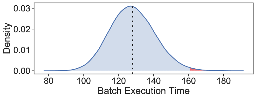
(a) Homogeneous gamma distribution model.

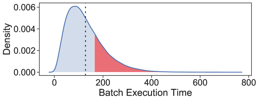
(b) Heterogeneous gamma distribution model.

Figure 3: Gamma-distribution in homogeneous and heterogeneous environments. The x-axis is the simulated time units the iteration takes while the y-axis is the probability. Both environments have the same mean (128 time units). The red area represents the probability to have an iteration which takes more than 1.25x longer than the mean iteration time.

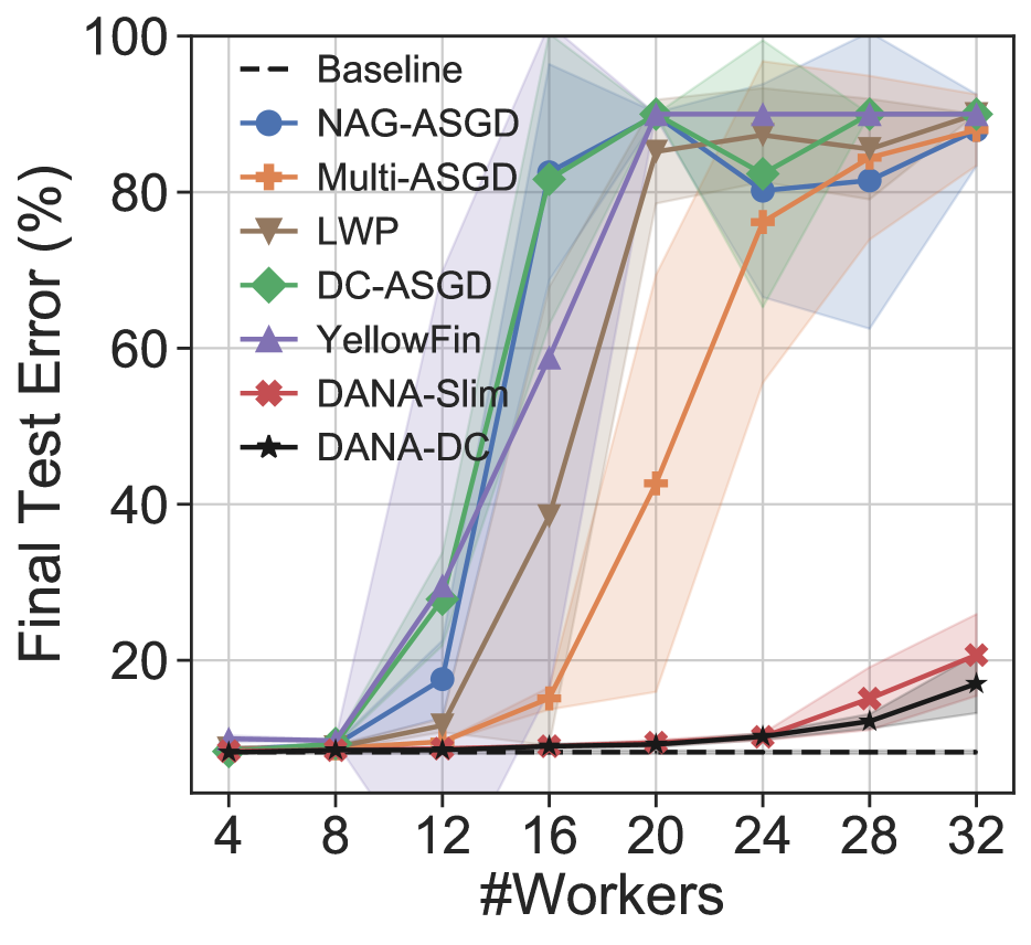
(a) CIFAR10 ResNet-20

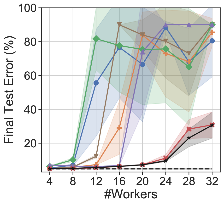
(b) CIFAR10 Wide ResNet 16-4

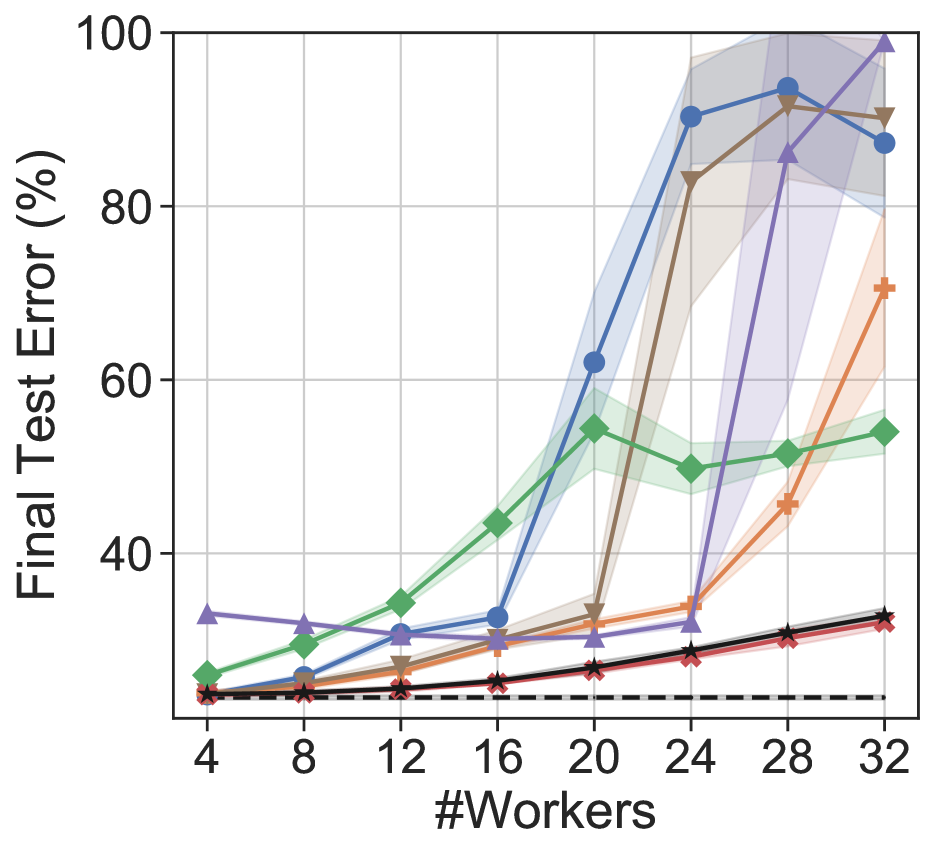
(c) CIFAR100 Wide ResNet 16-4

Figure 4: Final test error for different numbers of workers $N$.

Simulation

We simulate the workers’ execution time using a gamma-distributed model (Ali et al., 2000), where the execution time for each individual batch is drawn from a gamma distribution. The gamma distribution is a well-accepted model for task execution time that naturally gives rise to stragglers. We use the formulation proposed by Ali et al. (2000) and set $V=0.1$ and $\mu=B*V^{2}$, where $B$ is the batch size, yielding a mean execution time of $B$ simulated time units (additional details in Section A.4). Figure 3 visualizes the distribution of workers’ batch execution time. As expected, stragglers appear much more frequently in the heterogeneous environment than in the homogeneous environment.

Since one of our main goals in these experiments is to verify that decreasing the gap leads to a better final test error and convergence rate, we use the same hyperparameters across all algorithms. These are the original hyperparameters suggested by the authors of each neural network architecture’s respective paper, tuned for a single worker (for additional details please see Section A.5). This eases the scaling to more workers since it doesn’t require re-tuning the hyperparameters when increasing the cluster size.

Algorithms

Our goal is to produce a scalable method that works well with momentum and therefore all evaluated algorithms use momentum (as does the baseline). Our evaluations consist of the following algorithms:

• Baseline: Single worker with the same tuned hyperparameters as in the respective neural network’s paper. This baseline does not suffer from gradient staleness, thus it is ideal in terms of final accuracy and convergence speed.

• NAG-ASGD: Asynchronous SGD, which uses a single NAG optimizer for all workers.

• Multi-ASGD: Asynchronous SGD, which maintains a separate NAG optimizer for each worker.

• DC-ASGD: Delay compensation asynchronous SGD, as described in Section 4.3, for which we set $\gamma=0.95$ as suggested by Zheng et al. (2017).

• YellowFin: An algorithm proposed by Zhang & Mitliagkas (2019), that automatically tunes the momentum $\gamma$ and learning rate $\eta$ throughout the training process. We used the asynchronous variation of YellowFin, named Closed-Loop, and set the hyperparameters $\eta=1e-4$ and $\gamma=0.0$ as suggested by Zhang & Mitliagkas (2019).

• LWP: Linear Weight Prediction, described in Section 3.1.

• DANA-Slim: A variation of DANA-Zero, which eliminates the overhead, as described in Section 4.2.

• DANA-DC: A combination of DANA-Zero with DC-ASGD, as described in Section 4.3, for which we set $\lambda=2$, as suggested by Zheng et al. (2017).

5.1 Evaluation on the CIFAR Datasets

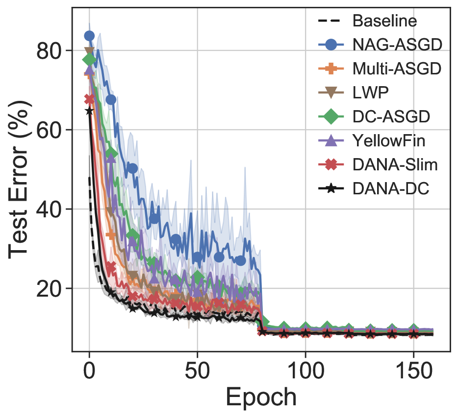
(a) CIFAR10 ResNet-20

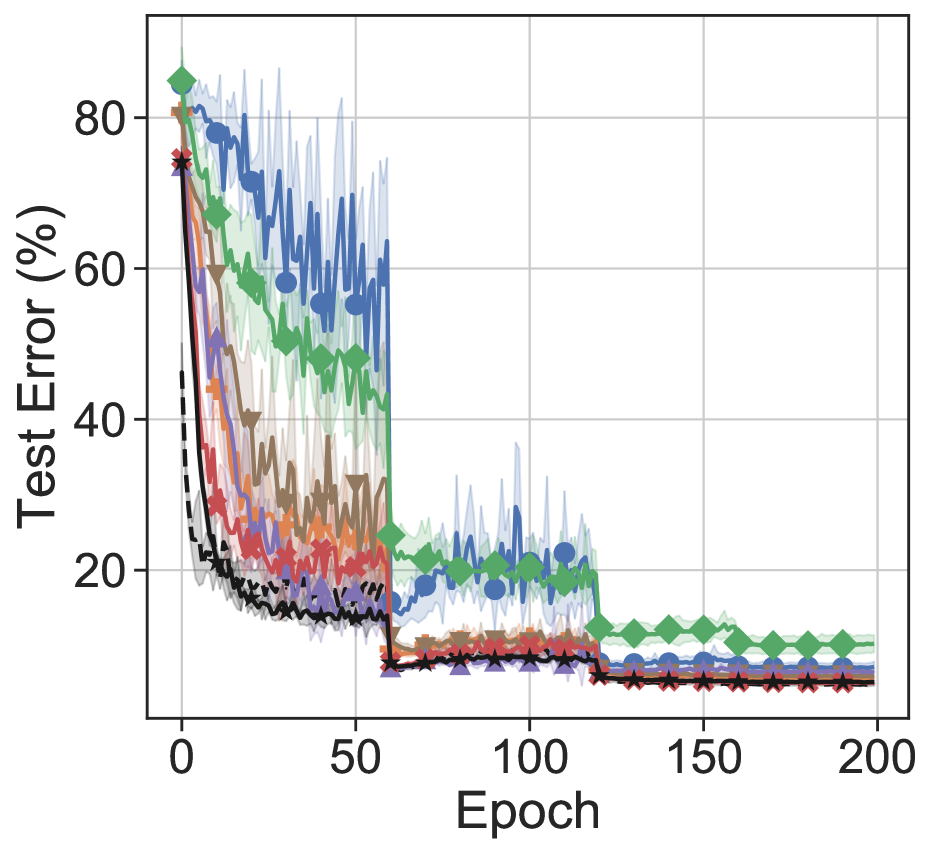
(b) CIFAR10 Wide ResNet 16-4

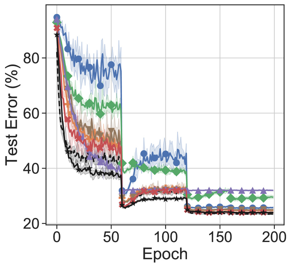
(c) CIFAR100 Wide ResNet 16-4

Figure 5: Convergence rate for 8 workers.

We evaluate DANA with the ResNet-20 (He et al., 2016) and Wide ResNet 16-4 (Zagoruyko & Komodakis, 2016) architectures on the CIFAR-10 and CIFAR-100 datasets (Hinton, 2007). In the CIFAR experiments, bold lines show the mean over five different runs with random seeds, while transparent bands show the standard deviation. The baseline is the mean of five different runs with a single worker.

Figure 4 shows that the final test error of both DANA-Slim and DANA-DC is lower than all the other algorithms for any number of workers, especially for large numbers of workers. Both variations of DANA exhibit a very small standard deviations, which points to the high stability DANA provides, even for large numbers of workers. The final accuracies of all the CIFAR experiments are listed in Section B.1.

NAG-ASGD demonstrates how gradient staleness is exacerbated by momentum. NAG-ASGD yields good accuracy with few workers, but fails to converge when trained with more than 16 workers. LWP scales better than NAG-ASGD but falls short of Multi-ASGD. Multi-ASGD serves as an ablation study: its poor scalability demonstrates that it is not sufficient to simply maintain a momentum vector for every worker. Hence, DANA (Section 4) is also required to achieve fast convergence and low test error.

Figure 5 shows the mean and standard deviation of the test error throughout the training of the different algorithms when trained on eight workers. This figure demonstrates the significantly better convergence rate of DANA-DC. It is usually similar to the baseline or even faster and outperforms all the other algorithms. It is noteworthy that DANA-DC’s convergence rate surpasses that of DANA-Slim; however, DANA-DC incurs an overhead and both algorithms usually reach a similar final test error, as seen in Figure 4.

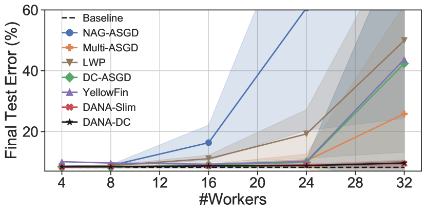
Figure 6: Final test error for different numbers of workers $N$ when training ResNet-20 on CIFAR10 in a heterogeneous environment.

When attempting to utilize different computational resources (Yang et al., 2018; 2020; Woodworth et al., 2020), workers may have considerably different computational power from one another. This heterogeneous environment creates high variance in batch execution times, as shown in Figure 3(b). Therefore, in heterogeneous environments, asynchronous algorithms have a distinct speedup advantage over synchronous algorithms which are slowed down by the slowest worker if not addressed (Dutta et al., 2018; Hanna et al., 2020). Figure 6 shows that even in heterogeneous environments, DANA achieves high final accuracy on large clusters of workers. For additional details about the heterogeneous experiments please see Appendix D.

5.2 Evaluation on the ImageNet Dataset

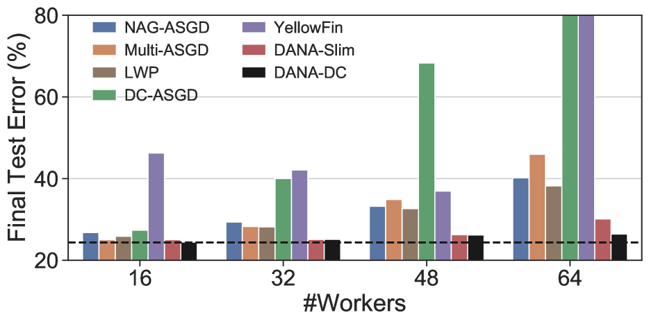
(a) Final test error on 16, 32, 48, and 64 workers

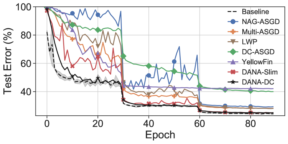
(b) Convergence rate on 32 workers

Figure 7: 7(a) and 7(b) show the final test errors and convergence speed, respectively, when training a ResNet-50 architecture on the ImageNet dataset. The black dashed line represents the baseline of a single worker.

Figure 7 shows experiments where we evaluate DANA with ResNet-50 (He et al., 2016) on the ImageNet dataset (Russakovsky et al., 2015). In this experiment, every asynchronous worker is a machine with 8 GPUs, so the 64-worker experiment simulates a total of 512 GPUs with a total batch size of 16K. Figure 7(a) compares final test errors on different cluster sizes and shows that the scalability in terms of final accuracy of DANA-Slim and DANA-DC is much greater than all the other algorithms. Figure 7(b) shows that both variations of DANA significantly outperform all the other algorithms in both convergence speed and final accuracy when trained on $32$ asynchronous workers. Section B.2 lists the final test accuracies on ImageNet.

5.3 The Importance of the Gap

Although all algorithms share the same average lag (for a given number of workers), the algorithms that achieve a lower average gap (Figure 2(b)) also demonstrate low final error (Figure 4) and fast convergence rate (Figure 5). Ergo, we conclude that the gap is more informative than the lag when battling gradient staleness and that gap reduction is paramount to asynchronous training. We note that the average gap of both DANA-Zero and DANA-DC is an order of magnitude smaller than that of NAG-ASGD and LWP, as shown in Figure 2(b). Further details of our analysis on the gap are discussed in Section B.3.

5.4 Evaluation on a Private Compute Cluster

While this work focuses on improving the accuracy of ASGD, we also measured acceleration in training time. We conduct our experiments on a system with $8$ Nvidia 2080ti GPUs that each have 11GB and base our code on PyTorch Paszke et al. (2019). We use an efficient implementation for synchronous training (DistibutedDataParallel known as SSGD) based on the Ring-AllReduce communication algorithm that is implemented by Nvidia’s NCCL collective communication package. Furthermore, in SSGD, we overlap its computations with communications to accelerate the training by over $15\%$ (Li et al., 2020).

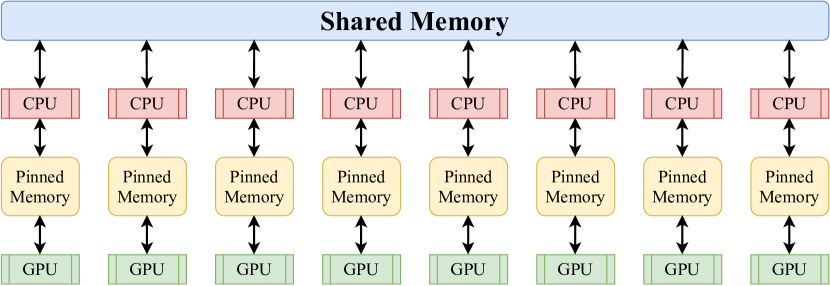
Figure 8: Our asynchronous lock-free training setup.

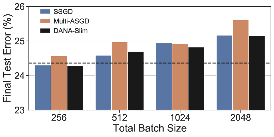
(a) Final test error on 256, 512, 1024, and 2048 total batch sizes

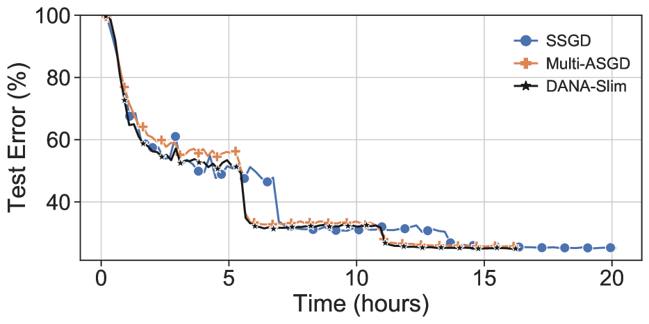
(b) Convergence rate on a total batch size of 2048

Figure 9: ImageNet ResNet-50 distributed training with 8 GPUs. The black dashed line in 9(a) represents the baseline with a single worker.

Table 1: Distributed results of ResNet-50 on ImageNet with an $8$ GPU machine (time in hours)

	DANA-Slim			Multi-ASGD			SSGD
Total Batch Size	Accuracy	Time	Speedup	Accuracy	Time	Speedup	Accuracy	Time	Speedup
256	75.71%	20.3	6.78x	75.44%	20.5	6.72x	75.7%	25.5	5.40x
512	75.31%	18	7.65x	75.03%	18	7.65x	75.42%	22.9	6.01x
1024	75.18%	16.9	8.15x	75.08%	16.9	8.15x	75.06%	20.9	6.59x
2048	74.85%	16.4	8.39x	74.39%	16.3	8.45x	74.84%	20.17	6.83x

Figure 8 shows our asynchronous training setup. Each worker is executed on a different process with a dedicated GPU. The shared parameters are stored and updated on the shared memory similar to Hogwild (Recht et al., 2011). The communications between the GPU and shared memory are transferred via pinned memory for fast parallel data transfer.

Figure 9 presents results when training the ResNet-50 architecture on ImageNet with different total batch sizes where every asynchronous worker is a single GPU. For total batch sizes that are larger than $256$ (batch size of $32$ per GPU) we use gradient accumulation Aji & Heafield (2019) to reduce memory footprint as well as reduce the synchronization frequency and communication overhead. Therefore, larger total batch sizes result in higher communication efficiency and shorter training times. Figure 9(a) compares the final test error on different total batch sizes. Multi-ASGD quickly drops in final accuracy when scaling the total batch size. DANA-Slim, on the other hand, not only scales well but in some cases even surpasses the final accuracy of SSGD. Figure 9(b) shows that DANA-Slim converges faster than both Multi-ASGD and SSGD. DANA-Slim trains $25\%$ faster than SSGD while achieving similar final accuracy. Table 1 lists the final accuracies, training time, and the speedup over a single GPU. DANA-Slim achieves perfect linear scaling while maintaining final accuracy similar to the baseline.

5.5 Evaluation on a Public Cloud Data-center

We evaluate the scalability of DANA-Slim on a public cloud data-center (Google cloud) with a single parameter server and one Nvidia Tesla V100 GPU per machine. Our cross-machine communications are based on CUDA-Aware MPI (OpenMPI) with a 10Gb Ethernet NIC per machine. Figure 10 shows that DANA-Slim successfully scales up to $20$ workers in agreement with the simulations of Figure 4(a) with high speedup and low final test error (less than $1\%$ higher than the baseline). We consider parameter server optimizations to be beyond the scope of this paper and detail popular parameter server optimization techniques that are orthogonal and compatible with DANA in Appendix C.

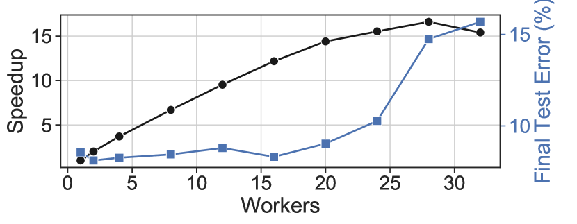
Figure 10: Speedup (solid line) and final test error (dashed) of DANA-Slim on CIFAR-10 using ResNet-20 on Google cloud. Each worker is one Nvidia V100 GPU with a $10$Gb Ethernet NIC.

6 Related Work

Asynchronous training causes gradient staleness, which hinders the convergence. Several approaches (Dai et al., 2019; Zhang et al., 2016; Zhou et al., 2018) proposed to mitigate gradient staleness by tuning the learning rate with regard to the lag $\tau$. These approaches are designed for SGD without momentum and therefore do not address the massive gap that momentum generates. Mitliagkas et al. (2016) show that asynchronous training induces implicit momentum. Thus, the momentum coefficient $\gamma$ must be decayed when scaling up the cluster size. By decreasing the gap caused by momentum, we show that fast convergence and high final test accuracy is possible in an asynchronous environment with DANA, even when $\gamma$ is relatively high.

Other approaches for mitigating gradient staleness include DC-ASGD (Zheng et al., 2017), which uses a Taylor expansion to reduce the gradient staleness. YellowFin (Zhang & Mitliagkas, 2019) is an SGD based algorithm that automatically tunes the momentum coefficient $\gamma$ and learning rate $\eta$ throughout the training process. Both YellowFin and DC-ASGD achieve high accuracy on small clusters, but fall short when trained on large clusters (Figure 4) due to the massive negative effects of the gradient staleness. Communication-efficient asynchronous algorithms, such as Elastic Averaging SGD (EASGD) by Zhang et al. (2015), can reduce communication overhead. EASGD is an asynchronous algorithm that uses a center force to pull the workers’ parameters towards the master’s parameters. This allows each worker to train asynchronously and synchronize with the master once every few iterations. Not only are these approaches compatible with (and indeed orthogonal to) DANA, we show that DANA can amplify the effectiveness of the other approaches, as demonstrated with DANA-DC (Section 4.3).

7 Conclusion

In this paper we tackle gradient staleness, one of the main difficulties in scaling SGD to large clusters in an asynchronous environment. We introduce DANA: a novel asynchronous distributed technique that mitigates gradient staleness by computing the gradient on an estimated future position of the model’s parameters. Despite using momentum, DANA efficiently scales to large clusters while maintaining high final accuracy and fast convergence. Thereby, we showed for the first time that momentum can be fully incorporated in asynchronous training with almost no ramifications to final accuracy. We performed an extensive set of evaluations on simulations, private compute clusters, and public cloud data-centers. Throughout our evaluations, DANA consistently outperformed all the other algorithms in both final test error and convergence rate. For future work, we plan on adapting DANA to newer optimizers, such as Nadam (Dozat, 2016), and to more recent asynchronous algorithms, in particular EASGD and YellowFin.

Appendix A Experimental Setup

A.1 Algorithms

Algorithms 8, 9 and 10 only change the master’s algorithm; the complementary worker algorithm is the same as ASGD (Algorithm 1). The master’s scheme is a simple FIFO. We consider parameter server optimizations to be beyond the scope of this paper.

Algorithm 8 NAG-ASGD: master

  Receive gradient $g^{i}$ from worker $i$

  Update momentum $v\leftarrow\gamma v+g^{i}$

  Update master’s weights $\theta^{0}\leftarrow\theta^{0}-\eta v$

  Send $\theta^{0}$ to worker $i$

Algorithm 9 Multi-ASGD: master

  Receive gradient $g^{i}$ from worker $i$

  Update momentum $v^{i}\leftarrow\gamma v^{i}+g^{i}$

  Update master’s weights $\theta^{0}\leftarrow\theta^{0}-\eta v^{i}$

  Send $\theta^{0}$ to worker $i$

Algorithm 10 DC-ASGD: master

  Receive gradient $g^{i}$ from worker $i$

  Update the gradient according to the delay compensation term $\hat{g}^{i}=g^{i}+\lambda g^{i}\odot g^{i}\odot(\theta^{0}-\theta^{i})$

  Update momentum $v^{i}\leftarrow\gamma v^{i}+\hat{g}^{i}$

  Update master’s weights $\theta^{0}\leftarrow\theta^{0}-\eta v^{i}$

  Send $\theta^{0}$ to worker $i$

A.2 Efficient computation in DANA-Zero

Computing the full summation $\sum_{i=1}^{N}v^{i}_{prev(i,t-1)}$ of the future position of the master’s parameters can be computationally expensive since its computational cost scales up with the number of workers. In practice, DANA-Zero doesn’t compute the full summation for every worker that requires the future position of the masters parameters. Instead, DANA-Zero maintains $v^{0}$, which is equivalent to the summation of all current momentum vectors at step $t$. After an update from worker $i$, DANA-Zero subtracts the worker’s previous momentum vector $v^{i}_{prev(i,t-1)}$ from $v^{0}_{t}$ and adds the worker’s updated momentum vector $v^{i}_{t}$ to $v^{0}_{t}$. Thus, after each worker update, $v^{0}_{t}$ is updated by $v^{0}_{t}=v^{0}_{t}-v^{i}_{prev(i,t-1)}+v^{i}_{t}$. Hence, the computation cost of the summation reduces from $\mathcal{O}(k\cdot N)$ to $\mathcal{O}(k)$; this is the same cost as computing the traditional NAG look-ahead, which isn’t affected by the number of workers $N$.

A.3 Datasets

CIFAR

The CIFAR-10 (Hinton, 2007) dataset comprises of 60K RGB images partitioned into 50K training images and 10K test images. Each image contains 32x32 RGB pixels and belongs to 1 of 10 equal-sized classes. CIFAR-100 is similar but contains 100 classes. Link.

ImageNet

The ImageNet dataset (Russakovsky et al., 2015), known as ILSVRC2012, consists of RGB images, each labeled as 1 of 1000 classes. Images are partitioned into 1.28 million training images and 50K validation images. Each image is randomly cropped and re-sized to 224x224 (1-crop validation). Link.

A.4 Gamma Distribution

Ali et al. (2000) suggest a method called CVB to simulate the run-time of a distributive network of computers. The method is based on several definitions: Task execution time variables:

• $\mu_{task}$ - mean time of tasks

• $V_{task}$ - variance of tasks

• $\mu_{mach}$ - mean computation power of machines

• $V_{mach}$ - variance of computation power of machines

• $\alpha_{task}=\frac{1}{V_{task}^{2}}$

• $\alpha_{mach}=\frac{1}{V_{mach}^{2}}$

$G(\alpha,\beta)$ is a random number generated using a gamma distribution, where $\alpha$ is the shape and $\beta$ is the scale.

For our case, all tasks are similar and run on a batch size of B. Therefore, the algorithm for deciding the execution-time of every task on a certain machine is reduced to one of the following:

Algorithm 11 Task execution time - homogeneous machines

  $\beta_{task}$ = $\frac{\mu_{task}}{\alpha_{task}}$

  $q=G(\alpha_{task},\beta_{task})$

  $\beta_{mach}=\frac{q}{\alpha_{mach}}$

  for i from 0 to $K-1$:

  $\quad time=G(\alpha_{mach},\beta_{mach})$

Algorithm 12 Task execution time - heterogeneous machines

  $\beta_{mach}$ = $\frac{\mu_{mach}}{\alpha_{mach}}$

  for j from 0 to $M$:

  $\quad p[j]=G(\alpha_{mach},\beta_{mach})$

  $\beta_{task}[j]=\frac{p[j]}{\alpha_{task}}$

  for i from 0 to $K-1$:

  $\quad time=G(\alpha_{task},\beta_{task}[curr])$

where $K$ is the total amount of tasks of all the machines combined (the total number of batch iterations), $M$ is the total number of machines (workers), and $curr$ is the machine currently about to run.

We note that Algorithms 11 and 12 naturally give rise to stragglers. In the homogeneous algorithm, all workers have the same mean execution time but some tasks can still be very slow; this generally means that in every epoch a different machine will be the slowest. In the heterogeneous algorithm, every machine has a different mean execution time throughout the training. We further note that $p[j]$ is the mean execution time of machine $j$ on the average task.

In our experiments, we simulated execution times using the following parameters as suggested by Ali et al. (2000): $\mu_{task}=\mu_{mach}=B\cdot V_{mach}^{2}$, where $B$ is the batch size, yielding a mean execution time of $\mu$ simulated time units, which is proportionate to $B$. In the homogeneous setting $V_{mach}=0.1$, whereas in the heterogeneous setting $V_{mach}=0.6$. For both settings, $V_{task}=0.1$.

Figure 3 illustrates the differences between the homogeneous and heterogeneous gamma-distribution. Both environments have the same mean (128) but the probability of having an iteration that is at least 1.25x longer than the mean (which means 160 or more) is significantly higher in the heterogeneous environment (27.9% in heterogeneous environment as opposed to 1% in the homogeneous environment).

A.5 Hyperparameters

To verify that decreasing the gap leads to a better final test error and convergence rate, especially when scaling to more workers, we used the same hyperparameters across all the tested algorithms. These hyperparameters are the original hyperparameters of the respective neural network architecture, which are tuned for a single worker.

CIFAR-10 ResNet-20

• Initial learning rate $\eta$: $0.1$

• Momentum coefficient $\gamma$: $0.9$ with NAG

• Dampening: $0$ (no dampening)

• Batch size $B$: $128$

• Weight decay: $1e-4$

• Learning rate decay: $0.1$

• Learning rate decay schedule: epochs $80$ and $120$

• Total epochs: $160$

CIFAR-10/100 Wide ResNet 16-4

• Initial learning rate $\eta$: $0.1$

• Momentum coefficient $\gamma$: $0.9$ with NAG

• Dampening: $0$ (no dampening)

• Batch size $B$: $128$

• Weight decay: $5e-4$

• Learning rate decay: $0.2$

• Learning rate decay schedule: epochs $60$, $120$ and $160$

• Total epochs: $200$

ImageNet ResNet-50

• Initial learning rate $\eta$: $0.1$

• Momentum coefficient $\gamma$: $0.9$ with NAG

• Dampening: $0$ (no dampening)

• Batch size $B$: $256$

• Weight decay: $1e-4$

• Learning rate decay: $0.1$

• Learning rate decay schedule: epochs $30$ and $60$

• Total epochs: $90$

Learning Rate Warm-Up

In the early stages of training, the network generally changes rapidly, causing error spikes. For all algorithms, we followed the gradual warm-up approach proposed by Goyal et al. (2017) to overcome this problem. We divided the initial learning rate by the number of workers $N$ and ramped it up linearly until it reached its original value after five epochs. We also used momentum correction (Goyal et al., 2017) in all algorithms to stabilize training when the learning rate changes.

Appendix B Additional Results

B.1 CIFAR Final Accuracies

DANA-DC starts to show signs of divergence when it reaches $32$. However, when we tuned the learning rate $\eta$, DANA-DC reached a significantly lower test error than that shown in Tables 2, 3 and 4. More precisely, when trained on $32$ workers with $\eta=0.025$, DANA-DC reached a test error of only 2.5% higher than the baseline on both CIFAR10 scenarios and 4.5% higher than the baseline on CIFAR100.

Table 2: ResNet-20 CIFAR10 Final Test Accuracy (Baseline 91.63%)

#Workers	DANA-DC	DANA-Slim	DC-ASGD	Multi-ASGD	NAG-ASGD	YellowFin
4	91.79 $\pm$ 0.21	91.65 $\pm$ 0.15	91.68 $\pm$ 0.18	91.55 $\pm$ 0.15	91.41 $\pm$ 0.23	90.05 $\pm$ 0.37
8	91.51 $\pm$ 0.16	91.52 $\pm$ 0.16	90.67 $\pm$ 0.26	91.28 $\pm$ 0.21	90.83 $\pm$ 0.18	90.29 $\pm$ 0.14
12	91.49 $\pm$ 0.18	91.32 $\pm$ 0.16	72.16 $\pm$ 5.32	90.42 $\pm$ 0.08	82.41 $\pm$ 4.41	90.54 $\pm$ 0.18
16	91.01 $\pm$ 0.25	91.02 $\pm$ 0.16	18.35 $\pm$ 16.7	84.88 $\pm$ 1.28	17.45 $\pm$ 12.39	41.19 $\pm$ 38.21
20	90.78 $\pm$ 0.32	90.56 $\pm$ 0.32	10.0 $\pm$ 0.0	57.32 $\pm$ 23.9	10.17 $\pm$ 0.33	10.0 $\pm$ 0.0
24	89.76 $\pm$ 0.37	89.81 $\pm$ 0.4	17.65 $\pm$ 15.3	23.83 $\pm$ 18.43	19.81 $\pm$ 12.2	10.0 $\pm$ 0.0
28	87.82 $\pm$ 0.83	84.91 $\pm$ 3.6	10.0 $\pm$ 0.0	15.58 $\pm$ 9.38	18.5 $\pm$ 17.0	10.0 $\pm$ 0.0
32	82.99 $\pm$ 3.38	79.33 $\pm$ 4.68	10.0 $\pm$ 0.0	12.04 $\pm$ 4.08	12.06 $\pm$ 4.11	10.0 $\pm$ 0.0

Table 3: Wide ResNet 16-4 CIFAR10 Final Test Accuracy (Baseline $95.17\%$)

#Workers	DANA-DC	DANA-Slim	DC-ASGD	Multi-ASGD	NAG-ASGD	YellowFin
4	95.08 $\pm$ 0.13	95.04 $\pm$ 0.11	93.66 $\pm$ 0.16	94.97 $\pm$ 0.11	94.81 $\pm$ 0.11	92.81 $\pm$ 0.04
8	94.84 $\pm$ 0.19	94.91 $\pm$ 0.2	89.76 $\pm$ 1.0	94.25 $\pm$ 0.12	92.83 $\pm$ 0.61	93.52 $\pm$ 0.08
12	94.35 $\pm$ 0.16	94.45 $\pm$ 0.21	18.24 $\pm$ 16.49	92.64 $\pm$ 0.17	44.35 $\pm$ 28.22	93.78 $\pm$ 0.08
16	93.67 $\pm$ 0.15	93.66 $\pm$ 0.2	22.29 $\pm$ 24.59	70.86 $\pm$ 14.08	23.36 $\pm$ 26.72	93.19 $\pm$ 0.18
20	92.73 $\pm$ 0.37	92.72 $\pm$ 0.13	24.59 $\pm$ 29.18	16.13 $\pm$ 12.25	33.41 $\pm$ 30.31	26.03 $\pm$ 32.06
24	90.4 $\pm$ 0.4	88.76 $\pm$ 1.85	24.27 $\pm$ 28.54	26.98 $\pm$ 23.0	11.62 $\pm$ 3.23	10.0 $\pm$ 0.0
28	76.88 $\pm$ 4.65	71.62 $\pm$ 5.0	34.92 $\pm$ 30.88	31.77 $\pm$ 26.66	31.91 $\pm$ 17.68	10.0 $\pm$ 0.0
32	69.35 $\pm$ 6.86	69.13 $\pm$ 6.85	10.0 $\pm$ 0.0	14.51 $\pm$ 7.4	19.52 $\pm$ 19.03	10.0 $\pm$ 0.0

Table 4: Wide ResNet 16-4 CIFAR100 Final Test Accuracy (Baseline $76.72\%$)

#Workers	DANA-DC	DANA-Slim	DC-ASGD	Multi-ASGD	NAG-ASGD	YellowFin
4	76.22 $\pm$ 0.15	76.27 $\pm$ 0.33	74.03 $\pm$ 0.26	76.07 $\pm$ 0.23	76.27 $\pm$ 0.2	66.91 $\pm$ 0.25
8	76.05 $\pm$ 0.23	76.07 $\pm$ 0.17	70.48 $\pm$ 0.48	75.33 $\pm$ 0.29	74.24 $\pm$ 0.27	68.05 $\pm$ 0.21
12	75.57 $\pm$ 0.24	75.64 $\pm$ 0.28	65.7 $\pm$ 0.68	73.63 $\pm$ 0.29	69.29 $\pm$ 0.56	69.36 $\pm$ 0.22
16	74.69 $\pm$ 0.28	74.97 $\pm$ 0.1	56.5 $\pm$ 1.75	70.68 $\pm$ 0.23	67.37 $\pm$ 0.74	69.85 $\pm$ 0.29
20	73.14 $\pm$ 0.58	73.48 $\pm$ 0.35	45.61 $\pm$ 4.16	68.12 $\pm$ 0.48	37.98 $\pm$ 7.21	69.62 $\pm$ 0.18
24	71.19 $\pm$ 0.32	71.91 $\pm$ 0.27	50.24 $\pm$ 2.63	66.12 $\pm$ 0.58	9.67 $\pm$ 4.89	67.9 $\pm$ 0.49
28	69.14 $\pm$ 0.62	69.77 $\pm$ 0.83	48.49 $\pm$ 1.31	54.3 $\pm$ 2.29	6.35 $\pm$ 7.41	13.76 $\pm$ 25.52
32	67.19 $\pm$ 0.79	67.91 $\pm$ 0.7	45.98 $\pm$ 2.26	29.43 $\pm$ 8.11	12.71 $\pm$ 7.69	1.0 $\pm$ 0.0

B.2 ImageNet Final Accuracies

Table 5: ResNet-50 ImageNet Final Test Accuracy (Baseline $75.64\%$)

#Workers	DANA-DC	DANA-Slim	DC-ASGD	Multi-ASGD	NAG-ASGD	YellowFin	LWP
16	75.54%	74.95%	72.64%	74.96%	73.22%	53.74%	74.12%
32	74.86%	74.89%	59.99%	71.72%	70.64%	57.88%	71.84%
48	73.80%	73.75%	31.71%	65.13%	66.78%	63.07%	67.34%
64	73.58%	69.88%	8.1%	54.04%	59.81%	0.15%	61.8%
128	69.50%	NaN	NaN	NaN	NaN	NaN	NaN

Table 5 lists the final test accuracy of the different algorithms when training the ResNet-50 architecture (He et al., 2016) on ImageNet. DANA consistently outperforms all the other algorithms.

B.3 Normalized Gap

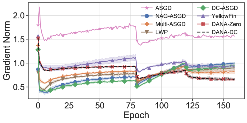
(a) Gradient norm.

(b) Normalized gap.

Figure 11: Figures 11(a) and 11(b) compare the different asynchronous algorithms when training the ResNet-20 architecture on the CIFAR-10 dataset with $8$ workers. Figures 11(a) and 11(b) show the gradient norm and the normalized gap, respectively, throughout the training process. The large drops in Figure 11(b) are caused by learning rate decay.

As shown in Figure 2(b), the gap of DANA-Zero is smaller than that of ASGD, despite Equation 12. This is because DANA-Zero uses momentum, which accelerates the convergence and leads to smaller gradients. To make a more accurate comparison between the gaps of different algorithms, we define the normalized gap as $\operatorname{G}^{*}(\Delta_{t+\tau})=\frac{\operatorname{G}(\Delta_{t+\tau})}{\lVert g_{t}\rVert}$. Figure 11(b) shows that the normalized gap of ASGD is roughly similar to that of DANA-Zero, empirically confirming Equation 12. This suggests that DANA-Zero’s future position approximation is close to optimal, even when training with stragglers.

Appendix C Asynchronous Speedup

C.1 CIFAR-10 Distributed Experiments

DANA-Slim successfully scales up to $20$ workers (similarly to the simulations) with high speedup and low final test error (less than $1\%$ higher than the baseline). Above $20$ workers, the master becomes a bottleneck. This is consistent with the literature on ASGD (Xing et al., 2015). To overcome this bottleneck, existing parameter server optimization techniques can be used, such as sharding (Dean et al., 2012; Li et al., 2014), synchronization frequency reduction (Wang & Joshi, 2018), network utilization improvements (Jia et al., 2018; Zhao et al., 2020; Wang et al., 2020), communication compression (Tang et al., 2019; Lim et al., 2018; Lin et al., 2018; Bernstein et al., 2018; Lim et al., 2019), and overlapping communications with computations (Hashemi et al., 2019; Jayarajan et al., 2019). We note that DANA is compatible with these optimizations. The speedup superiority of ASGD methods compared to SSGD methods is discussed in Appendix C.

Figure 10 shows the speedup and final test error when running DANA-Slim on the Google Cloud Platform with a single parameter server (master) and one Nvidia Tesla V100 GPU per machine, when training ResNet-20 on the CIFAR-10 dataset. It shows speedup of up to $16\times$ when training with $N=24$ workers. As before, its final test error remains close to the baseline for up to $N=24$ workers.

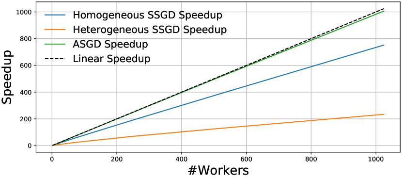
(a) ASGD and SSGD speedups.

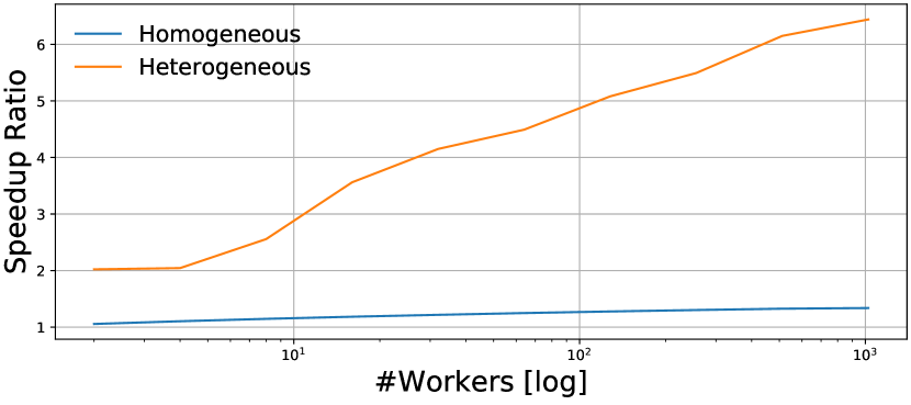
(b) ASGD speedup over SSGD. X axis is in log scale.

Figure 12: Theoretical speedups for any ASGD (such as DANA) and SSGD algorithms when batch execution times are drawn from a gamma distribution. Communication overheads aren’t modeled. Since ASGD is more efficient in communication, accounting for the communication overheads should expand the gap between the ASGD and SSGD, in favor of ASGD.

Cloud computing is becoming increasingly popular as a platform to perform distributed training of deep neural networks (Or et al., 2020). Although synchronous SGD is currently the primary method (Mikami et al., 2018; Ying et al., 2018; Yamazaki et al., 2019; Goyal et al., 2017; Luo et al., 2020) used to distribute the learning process, it suffers from substantial slowdowns when run in non-dedicated environments such as the cloud. This shortcoming is magnified in heterogeneous environments and non-dedicated networks. ASGD addresses the SSGD drawback and enjoys linear speedup in terms of the number of workers in both heterogeneous and homogeneous environments even in non-dedicated networks. This makes ASGD a potentially better alternative for cloud computing.

Figure 12(a) shows the theoretically achievable speedup, based on the detailed gamma-distributed model, for asynchronous (GA and other ASGD variants) and synchronous algorithms using homogeneous and heterogeneous workers. The asynchronous algorithms can achieve linear speedup while the synchronous algorithm (SSGD) falls short as we increase the number of workers. This occurs because SSGD must wait in each iteration until all workers complete their batch. Figure 12(b) shows that ASGD-based algorithms (including GA, SA and DANA versions) are up to $21\%$ faster than SSGD in homogeneous environments. In heterogeneous environments, ASGD methods can be 6x faster than SSGD. We note that this speedup is an underestimate, since our simulation includes only batch execution times. It does not model the execution time of barriers, all-gather operations, and other overheads which usually increase communication time, especially in SSGD.

Appendix D Heterogeneous Environment

(a) Final test error for different numbers of workers $N$.

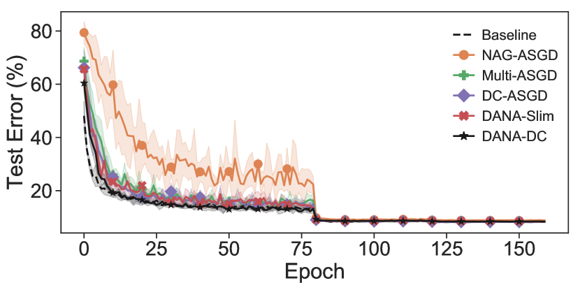
(b) Convergence rate for 8 workers.

Figure 13: Training of ResNet-20 on CIFAR10 in a heterogeneous environment.

In our experiments, the algorithms scale better in the heterogeneous environment Figure 13(a) than in the homogeneous environment (Figure 4(a)). The reason is that stragglers naturally have less impact on the training process. We will demonstrate this with a simplistic example. Consider an asynchronous environment with only $N=2$ workers, where one worker is significantly faster than the other. The fast worker will run as in sequential SGD, since its gap and lag will mostly be zero. Conversely, the slow workers will have minimal impact and therefore its stale gradients wouldn’t harm the convergence process.

This suggests that high accuracy can be attained more easily in asynchronous heterogeneous environments than in homogeneous environments. Figures 13(a) and 13(b) show that even in a heterogeneous environment, DANA-DC converges the fastest and achieves the highest final accuracy. The final accuracies are listed in Table 6 below.

Table 6: Heterogeneous Environment ResNet 20 CIFAR10 Final Test Accuracy (Baseline 91.63%)

#Workers	DANA-DC	DANA-Slim	DC-ASGD	Multi-ASGD	NAG-ASGD
4	91.57 $\pm$ 0.14	91.7 $\pm$ 0.18	91.6 $\pm$ 0.14	91.77 $\pm$ 0.22	91.38 $\pm$ 0.12
8	91.57 $\pm$ 0.18	91.55 $\pm$ 0.28	91.72 $\pm$ 0.21	91.59 $\pm$ 0.11	91.15 $\pm$ 0.23
16	91.28 $\pm$ 0.21	91.31 $\pm$ 0.17	90.98 $\pm$ 0.5	91.12 $\pm$ 0.3	83.65 $\pm$ 5.17
24	91.21 $\pm$ 0.19	90.94 $\pm$ 0.27	90.11 $\pm$ 0.92	89.6 $\pm$ 2.03	39.36 $\pm$ 36.01
32	90.33 $\pm$ 0.58	90.52 $\pm$ 1.04	57.62 $\pm$ 38.93	74.18 $\pm$ 32.1	37.52 $\pm$ 34.12

References

- Aji & Heafield (2019) Aji, A. F. and Heafield, K. Making asynchronous stochastic gradient descent work for transformers. In Proceedings of the 3rd Workshop on Neural Generation and Translation, 2019.
- Ali et al. (2000) Ali, S., Siegel, H. J., Maheswaran, M., Ali, S., and Hensgen, D. Task execution time modeling for heterogeneous computing systems. In Proceedings of the 9th Heterogeneous Computing Workshop, 2000.
- Barkai et al. (2020) Barkai, S., Hakimi, I., and Schuster, A. Gap-aware mitigation of gradient staleness. In International Conference on Learning Representations, 2020.
- Ben-Nun & Hoefler (2019) Ben-Nun, T. and Hoefler, T. Demystifying parallel and distributed deep learning: An in-depth concurrency analysis. ACM Computing Surveys (CSUR), 2019.
- Bengio et al. (2013) Bengio, Y., Boulanger-Lewandowski, N., and Pascanu, R. Advances in optimizing recurrent networks. In IEEE International Conference on Acoustics, Speech and Signal Processing, 2013.
- Bernstein et al. (2018) Bernstein, J., Wang, Y.-X., Azizzadenesheli, K., and Anandkumar, A. signSGD: Compressed optimisation for non-convex problems. In Proceedings of the 35th International Conference on Machine Learning. PMLR, 2018.
- Chen et al. (2018) Chen, C.-C., Yang, C.-L., and Cheng, H.-Y. Efficient and robust parallel dnn training through model parallelism on multi-gpu platform. arXiv preprint arXiv:1809.02839, 2018.
- Chen et al. (2016) Chen, J., Pan, X., Monga, R., Bengio, S., and Jozefowicz, R. Revisiting distributed synchronous sgd. arXiv preprint arXiv:1604.00981, 2016.
- Cho et al. (2019) Cho, M., Finkler, U., Kung, D., and Hunter, H. Blueconnect: Decomposing all-reduce for deep learning on heterogeneous network hierarchy. In Talwalkar, A., Smith, V., and Zaharia, M. (eds.), Proceedings of Machine Learning and Systems. 2019.
- Cui et al. (2016) Cui, H., Zhang, H., Ganger, G. R., Gibbons, P. B., and Xing, E. P. Geeps: Scalable deep learning on distributed gpus with a gpu-specialized parameter server. In Proceedings of the Eleventh European Conference on Computer Systems, 2016.
- Dai et al. (2019) Dai, W., Zhou, Y., Dong, N., Zhang, H., and Xing, E. Toward understanding the impact of staleness in distributed machine learning. In International Conference on Learning Representations, 2019.
- Dean et al. (2012) Dean, J., Corrado, G., Monga, R., Chen, K., Devin, M., Le, Q. V., Mao, M. Z., Ranzato, M., Senior, A. W., Tucker, P. A., Yang, K., and Ng, A. Y. Large scale distributed deep networks. In Advances in Neural Information Processing Systems 25: 26th Annual Conference on Neural Information Processing Systems, 2012.
- Dozat (2016) Dozat, T. Incorporating Nesterov momentum into Adam. ICLR Workshop, 2016.
- Dutta et al. (2018) Dutta, S., Joshi, G., Ghosh, S., Dube, P., and Nagpurkar, P. Slow and stale gradients can win the race: Error-runtime trade-offs in distributed sgd. Proceedings of Machine Learning Research. PMLR, 2018.
- Goh (2017) Goh, G. Why momentum really works. Distill, 2017. doi: 10.23915/distill.00006. URL http://distill.pub/2017/momentum.
- Goyal et al. (2017) Goyal, P., Dollár, P., Girshick, R., Noordhuis, P., Wesolowski, L., Kyrola, A., Tulloch, A., Jia, Y., and He, K. Accurate, large minibatch sgd: Training imagenet in 1 hour. arXiv preprint arXiv:1706.02677, 2017.
- Guan et al. (2019) Guan, L., Yin, W., Li, D., and Lu, X. Xpipe: Efficient pipeline model parallelism for multi-gpu dnn training. arXiv preprint arXiv:1911.04610, 2019.
- Hanna et al. (2020) Hanna, S. K., Bitar, R., Parag, P., Dasari, V., and El Rouayheb, S. Adaptive distributed stochastic gradient descent for minimizing delay in the presence of stragglers. In ICASSP 2020-2020 IEEE International Conference on Acoustics, Speech and Signal Processing (ICASSP). IEEE, 2020.
- Hashemi et al. (2019) Hashemi, S. H., Abdu Jyothi, S., and Campbell, R. Tictac: Accelerating distributed deep learning with communication scheduling. In Talwalkar, A., Smith, V., and Zaharia, M. (eds.), Proceedings of Machine Learning and Systems. 2019.
- He et al. (2016) He, K., Zhang, X., Ren, S., and Sun, J. Deep residual learning for image recognition. In 2016 IEEE Conference on Computer Vision and Pattern Recognition, 2016.
- Hinton (2007) Hinton, G. E. Learning multiple layers of representation. Trends in Cognitive Sciences, 2007.
- Jayarajan et al. (2019) Jayarajan, A., Wei, J., Gibson, G., Fedorova, A., and Pekhimenko, G. Priority-based parameter propagation for distributed dnn training. In Talwalkar, A., Smith, V., and Zaharia, M. (eds.), Proceedings of Machine Learning and Systems. 2019.
- Jia et al. (2018) Jia, Z., Zaharia, M., and Aiken, A. Beyond data and model parallelism for deep neural networks. arXiv preprint arXiv:1807.05358, 2018.
- Keskar et al. (2016) Keskar, N. S., Mudigere, D., Nocedal, J., Smelyanskiy, M., and Tang, P. T. P. On large-batch training for deep learning: Generalization gap and sharp minima. arXiv preprint arXiv:1609.04836, 2016.
- Kosson et al. (2020) Kosson, A., Chiley, V., Venigalla, A., Hestness, J., and Köster, U. Pipelined backpropagation at scale: Training large models without batches. arXiv preprint arXiv:2003.11666, 2020.
- Lerer et al. (2019) Lerer, A., Wu, L., Shen, J., Lacroix, T., Wehrstedt, L., Bose, A., and Peysakhovich, A. Pytorch-biggraph: A large scale graph embedding system. In Talwalkar, A., Smith, V., and Zaharia, M. (eds.), Proceedings of Machine Learning and Systems, pp. 120–131. 2019.
- Li et al. (2014) Li, M., Andersen, D. G., Park, J. W., Smola, A. J., Ahmed, A., Josifovski, V., Long, J., Shekita, E. J., and Su, B.-Y. Scaling distributed machine learning with the parameter server. In 11th USENIX Symposium on Operating Systems Design and Implementation (OSDI 14), 2014.
- Li et al. (2020) Li, S., Zhao, Y., Varma, R., Salpekar, O., Noordhuis, P., Li, T., Paszke, A., Smith, J., Vaughan, B., Damania, P., et al. Pytorch distributed: experiences on accelerating data parallel training. arXiv preprint arXiv:2006.15704, 2020.
- Lim et al. (2018) Lim, H., Andersen, D. G., and Kaminsky, M. 3lc: Lightweight and effective traffic compression for distributed machine learning. arXiv preprint arXiv:1802.07389, 2018.
- Lim et al. (2019) Lim, H., Andersen, D. G., and Kaminsky, M. 3lc: Lightweight and effective traffic compression for distributed machine learning. In Talwalkar, A., Smith, V., and Zaharia, M. (eds.), Proceedings of Machine Learning and Systems. 2019.
- Lin et al. (2018) Lin, Y., Han, S., Mao, H., Wang, Y., and Dally, B. Deep gradient compression: Reducing the communication bandwidth for distributed training. In International Conference on Learning Representations, 2018.
- Loizou & Richtárik (2017a) Loizou, N. and Richtárik, P. Linearly convergent stochastic heavy ball method for minimizing generalization error. CoRR, abs/1710.10737, 2017a.
- Loizou & Richtárik (2017b) Loizou, N. and Richtárik, P. Momentum and stochastic momentum for stochastic gradient, newton, proximal point and subspace descent methods. CoRR, abs/1712.09677, 2017b.
- Luo et al. (2020) Luo, L., West, P., Nelson, J., Krishnamurthy, A., and Ceze, L. Plink: Discovering and exploiting locality for accelerated distributed training on the public cloud. In Dhillon, I., Papailiopoulos, D., and Sze, V. (eds.), Proceedings of Machine Learning and Systems. 2020.
- Mikami et al. (2018) Mikami, H., Suganuma, H., U.-Chupala, P., Tanaka, Y., and Kageyama, Y. Imagenet/resnet-50 training in 224 seconds. CoRR, abs/1811.05233, 2018. URL http://arxiv.org/abs/1811.05233.
- Mitliagkas et al. (2016) Mitliagkas, I., Zhang, C., Hadjis, S., and Ré, C. Asynchrony begets momentum, with an application to deep learning. In 54th Annual Allerton Conference on Communication, Control, and Computing, 2016.
- Narayanan et al. (2019) Narayanan, D., Harlap, A., Phanishayee, A., Seshadri, V., Devanur, N. R., Ganger, G. R., Gibbons, P. B., and Zaharia, M. Pipedream: generalized pipeline parallelism for dnn training. In Proceedings of the 27th ACM Symposium on Operating Systems Principles, 2019.
- Nesterov (1983) Nesterov, Y. A method of solving a convex programming problem with convergence rate o(1/k2). In Soviet Mathematics Doklady, 1983.
- Or et al. (2020) Or, A., Zhang, H., and Freedman, M. Resource elasticity in distributed deep learning. In Dhillon, I., Papailiopoulos, D., and Sze, V. (eds.), Proceedings of Machine Learning and Systems. 2020.
- Paszke et al. (2019) Paszke, A., Gross, S., Massa, F., Lerer, A., Bradbury, J., Chanan, G., Killeen, T., Lin, Z., Gimelshein, N., Antiga, L., et al. Pytorch: An imperative style, high-performance deep learning library. In Advances in neural information processing systems, 2019.
- Peng et al. (2019) Peng, Y., Zhu, Y., Chen, Y., Bao, Y., Yi, B., Lan, C., Wu, C., and Guo, C. A generic communication scheduler for distributed dnn training acceleration. In Proceedings of the 27th ACM Symposium on Operating Systems Principles, 2019.
- Polyak (1964) Polyak, B. Some methods of speeding up the convergence of iteration methods. USSR Computational Mathematics and Mathematical Physics, 1964.
- Raffel et al. (2019) Raffel, C., Shazeer, N., Roberts, A., Lee, K., Narang, S., Matena, M., Zhou, Y., Li, W., and Liu, P. J. Exploring the limits of transfer learning with a unified text-to-text transformer. arXiv preprint arXiv:1910.10683, 2019.
- Recht et al. (2011) Recht, B., Re, C., Wright, S., and Niu, F. Hogwild: A lock-free approach to parallelizing stochastic gradient descent. In Advances in neural information processing systems, 2011.
- Russakovsky et al. (2015) Russakovsky, O., Deng, J., Su, H., Krause, J., Satheesh, S., Ma, S., Huang, Z., Karpathy, A., Khosla, A., Bernstein, M. S., Berg, A. C., and Li, F. ImageNet large scale visual recognition challenge. International Journal of Computer Vision, 2015.
- Silver et al. (2016) Silver, D., Huang, A., Maddison, C. J., Guez, A., Sifre, L., van den Driessche, G., Schrittwieser, J., Antonoglou, I., Panneershelvam, V., Lanctot, M., Dieleman, S., Grewe, D., Nham, J., Kalchbrenner, N., Sutskever, I., Lillicrap, T. P., Leach, M., Kavukcuoglu, K., Graepel, T., and Hassabis, D. Mastering the game of go with deep neural networks and tree search. Nature, 2016.
- Sutskever et al. (2013) Sutskever, I., Martens, J., Dahl, G. E., and Hinton, G. E. On the importance of initialization and momentum in deep learning. In Proceedings of the 30th International Conference on Machine Learning, 2013.
- Tang et al. (2019) Tang, H., Yu, C., Lian, X., Zhang, T., and Liu, J. Doublesqueeze: Parallel stochastic gradient descent with double-pass error-compensated compression. In International Conference on Machine Learning, 2019.
- Wang et al. (2020) Wang, G., Venkataraman, S., Phanishayee, A., Devanur, N., Thelin, J., and Stoica, I. Blink: Fast and generic collectives for distributed ml. In Dhillon, I., Papailiopoulos, D., and Sze, V. (eds.), Proceedings of Machine Learning and Systems. 2020.
- Wang & Joshi (2018) Wang, J. and Joshi, G. Adaptive communication strategies to achieve the best error-runtime trade-off in local-update sgd. arXiv preprint arXiv:1810.08313, 2018.
- Woodworth et al. (2020) Woodworth, B., Patel, K. K., and Srebro, N. Minibatch vs local sgd for heterogeneous distributed learning. arXiv preprint arXiv:2006.04735, 2020.
- Xing et al. (2015) Xing, E. P., Ho, Q., Dai, W., Kim, J. K., Wei, J., Lee, S., Zheng, X., Xie, P., Kumar, A., and Yu, Y. Petuum: A new platform for distributed machine learning on big data. IEEE Transactions on Big Data, 2015.
- Yamazaki et al. (2019) Yamazaki, M., Kasagi, A., Tabuchi, A., Honda, T., Miwa, M., Fukumoto, N., Tabaru, T., Ike, A., and Nakashima, K. Yet another accelerated SGD: resnet-50 training on imagenet in 74.7 seconds. CoRR, abs/1903.12650, 2019. URL http://arxiv.org/abs/1903.12650.
- Yang et al. (2018) Yang, E., Kim, S.-H., Kim, T.-W., Jeon, M., Park, S., and Youn, C.-H. An adaptive batch-orchestration algorithm for the heterogeneous gpu cluster environment in distributed deep learning system. In 2018 IEEE International Conference on Big Data and Smart Computing (BigComp). IEEE, 2018.
- Yang et al. (2020) Yang, E., Kang, D.-K., and Youn, C.-H. Boa: batch orchestration algorithm for straggler mitigation of distributed dl training in heterogeneous gpu cluster. The Journal of Supercomputing, 2020.
- Ying et al. (2018) Ying, C., Kumar, S., Chen, D., Wang, T., and Cheng, Y. Image classification at supercomputer scale. CoRR, abs/1811.06992, 2018. URL http://arxiv.org/abs/1811.06992.
- You et al. (2020) You, Y., Li, J., Reddi, S., Hseu, J., Kumar, S., Bhojanapalli, S., Song, X., Demmel, J., Keutzer, K., and Hsieh, C.-J. Large batch optimization for deep learning: Training bert in 76 minutes. In International Conference on Learning Representations, 2020.
- Zagoruyko & Komodakis (2016) Zagoruyko, S. and Komodakis, N. Wide residual networks. In Proceedings of the British Machine Vision Conference, 2016.
- Zhang & Mitliagkas (2019) Zhang, J. and Mitliagkas, I. Yellowfin and the art of momentum tuning. In Talwalkar, A., Smith, V., and Zaharia, M. (eds.), Proceedings of Machine Learning and Systems. 2019.
- Zhang et al. (2015) Zhang, S., Choromanska, A., and LeCun, Y. Deep learning with elastic averaging SGD. In Advances in Neural Information Processing Systems 28: Annual Conference on Neural Information Processing Systems, 2015.
- Zhang et al. (2016) Zhang, W., Gupta, S., Lian, X., and Liu, J. Staleness-aware async-SGD for distributed deep learning. In Proceedings of the Twenty-Fifth International Joint Conference on Artificial Intelligence, 2016.
- Zhao et al. (2020) Zhao, W., Xie, D., Jia, R., Qian, Y., Ding, R., Sun, M., and Li, P. Distributed hierarchical gpu parameter server for massive scale deep learning ads systems. In Dhillon, I., Papailiopoulos, D., and Sze, V. (eds.), Proceedings of Machine Learning and Systems. 2020.
- Zheng et al. (2017) Zheng, S., Meng, Q., Wang, T., Chen, W., Yu, N., Ma, Z., and Liu, T. Asynchronous stochastic gradient descent with delay compensation. In Proceedings of the 34th International Conference on Machine Learning, 2017.
- Zhou et al. (2018) Zhou, Z., Mertikopoulos, P., Bambos, N., Glynn, P., Ye, Y., Li, L.-J., and Fei-Fei, L. Distributed asynchronous optimization with unbounded delays: How slow can you go? In Proceedings of the 35th International Conference on Machine Learning, 2018.