Simultaneous 22 GHz Water and 44 GHz Methanol Masers Survey of Ultracompact Hii Regions

Abstract

We have carried out a multi-epoch simultaneous survey of 22 GHz H₂O and 44 GHz Class I CH₃OH masers toward 103 ultracompact Hii regions (UCHiis) between 2010 and 2017. We detected H₂O and CH₃OH  maser emission in 74 (72%) and 55 (53%) UCHiis, respectively. Among them, 3 H₂O and 27 CH₃OH maser sources are new detections. These high detection rates suggest that the occurrence periods of both maser species are significantly overlapped with the UCHii phase of massive star formation. The CH₃OH maser lines always have small ($<$ 10 km s^-1) relative velocities with respect to the natal molecular cores, while H₂O maser lines often show larger relative velocities. Twenty four H₂O maser-detected sources have maser lines at relative velocities $>$ 30 km s^-1, and thirteen of them show extremely high-velocity ($>$ 50 km s^-1) components. The appearance and disappearance of H₂O maser lines are quite frequent over six-month or one-year time intervals. In contrast, CH₃OH maser lines usually do not exhibit significant variations in the line intensity, velocity, or shape for the same periods. The isotropic luminosities of both masers appear to correlate with the bolometric luminosities of the central stars. This correlation becomes much stronger in the case that data points in the low- and intermediate-mass regimes are added. The maser luminosities also tend to increase with the radio continuum luminosities of UCHiis and the submillimeter continuum luminosities of the associated dense cores.

1 INTRODUCTION

Various maser species are detected in star-forming regions and used to understand the fundamental processes of star formation, such as accretion disks, jets/outflows, and inflows. Water (H₂O), methanol (CH₃OH), and hydroxyl (OH) masers are the major maser species associated with star-forming regions. H₂O and OH masers are observed both in star-forming regions and evolved stars, while CH₃OH masers are exclusively detected in star-forming regions, especially high-mass ($>$ 8 M_⊙) star-forming regions (e.g., Garay & Lizano 1999; Breen et al. 2013; Urquhart et al. 2015). H₂O masers at 22 GHz frequency have been extensively studied since the first discovery by Cheung et al. (1969) in the interstellar medium. They are detected in a number of star-forming regions. In low- and intermediate-mass star-forming regions, H₂O masers are mostly associated with protostars (Class 0/I objects), while they are rarely detected in pre-main-sequence stars (Furuya et al., 2003; Bae et al., 2011). In high-mass star-forming regions, on the other hand, the masers are detected in a wide range of evolutionary stages, from protostellar objects to ultracompact Hii regions (UCHiis), the central stars of which have already reached the main-sequence stage (e.g., Churchwell et al. 1990; Hofner & Churchwell 1996; Beuther et al. 2002; Urquhart et al. 2009, 2011; Kim et al. 2018a). Elitzur et al. (1989) suggested, through detailed numerical calculations, that H₂O masers could be generated by collisional pumping in the post-shocked regions with unusually high gas temperature and density ($T_{\rm kin}\,\sim\,$500 K and $n_{\rm H_{2}}\,\sim\,10^{9}$ cm^-3). H₂O masers were observed to be closely related to outflows (Felli et al., 1992). High-resolution observations show that they are distributed in the immediate vicinity of the central stars and usually trace inner jets/outflows (e.g., Torrelles et al. 1997, 2011; Goddi & Moscadelli 2006). The H₂O maser luminosity has been found to increase with the bolometric luminosity of the central star (Wouterloot & Walmsley, 1986; Palla et al., 1991, 1993; Felli et al., 1992; Wilking et al., 1994; Furuya et al., 2003; Bae et al., 2011).

There are more than 40 CH₃OH molecular transitions, which have been observed to show maser emission (Müller et al., 2004). The CH₃OH maser transitions were divided into two groups, Class I and Class II, based on their association with other star formation indicators, such as IRAS point sources, UCHiis, high-mass protostellar objects (HMPOs), hot molecular cores (HMCs), H₂O maser sources, and so on (Menten, 1991). Class II CH₃OH masers are more spatially correlated with other star formation indicators, while Class I CH₃OH masers tend to have offsets from those indicators. Kurtz et al. (2004) found offsets of 0.1$-$1 pc between 44 GHz Class I CH₃OH masers and UCHiis in their subarcsecond-resolution observations using the Very Large Array (VLA). According to theoretical studies (Menten, 1996; Sobolev et al., 2007; Cragg et al., 2005), Class I CH₃OH masers can be produced by collisional pumping in regions with $T_{\rm kin}\sim\,$100 K and $n_{\rm H_{2}}\sim\,$10⁵ cm^-3, whereas Class II CH₃OH masers can be excited by radiation pumping in hotter and denser regions ($T_{\rm kin}\sim\,$150 K and $n_{\rm H_{2}}\sim\,$10⁷ cm^-3). These results suggest that the emitting regions of the two classes of maser emission are different. Interferometric observations show that Class II masers originate from accretion disks and inner jets (e.g., Bartkiewicz et al. 2009, 2011), while Class I masers emanate from the interacting regions of jets/outflows with the ambient dense molecular gas (e.g., Plambeck & Menten 1990; Kurtz et al. 2004). The most well-known CH₃OH maser lines in Class I include 44 GHz ($7_{0}-6_{1}\,A^{+}$) and 95 GHz ($8_{0}-7_{1}~{}A^{+}$) transitions and in Class II contain 6.7 GHz ($5_{1}-6_{0}\,A^{+}$) and 12.2 GHz ($2_{0}-3_{1}\,E$) transitions.

UCHiis are very small and dense hydrogen ionized gas regions with diameters $\lesssim$ 0.1 pc, electron densities ($n_{e}$) $\gtrsim$ 10⁴ cm^-3 and emission measures (EM) $\gtrsim$ 10⁷ pc cm^-6 (Wood & Churchwell 1989a, hereafter WC89a; Kurtz et al. 1994, hereafter KCW94). They are not only strong radio sources but also bright infrared sources, suggesting that they are still deeply embedded in the parental molecular clouds. Since they can be produced only by O- or early B-type stars, they have been believed to be prominent signposts of massive star-forming sites. In fact, Shepherd & Churchwell (1996) showed that many UCHiis are associated with bipolar molecular outflows, which are salient indicators of star formation. The vast majority of them are also associated with masers of H₂O, CH₃OH, and/or OH (see Garay & Lizano 1999 for a review).

In this paper, we present a multi-epoch simultaneous survey of 22 GHz H₂O and 44 GHz Class I CH₃OH masers toward 103 UCHiis. Particularly, the present survey provides a new 44 GHz CH₃OH maser catalog covering a large sample of UCHiis, with much higher sensitivities than most previous single-dish surveys. The primary scientific goal of this survey is to investigate the characteristics of the two maser species associated with UCHiis and to examine the relationship between these maser species and the evolutionary sequence of massive star formation. The source selection and observational details are described in § 2.1 and §  2.2, respectively. We present the results in § 3 and comments on some interesting individual sources in § 4. In § 5, we compare properties of the two masers with those of the central stars and host clumps and discuss the implications for the evolutionary sequence of massive star formation. The main results are summarized in § 6.

2 OBSERVATIONS

2.1 Source Selection

We selected 103 UCHiis from the catalogs of WC89a and KCW94. WC89a performed subarcsecond-resolution radio continuum observations with the VLA toward 80 compact Hii regions and complexes at 2 and 6 cm wavelengths. They detected at least one UCHii in each of 53 regions. Wood & Churchwell (1989b) found that all known UCHiis at that time have characteristic IRAS colors, Log$(F_{\rm 60}/F_{\rm 12})\,\geq\,1.30$ and Log$(F_{\rm 25}/F_{\rm 12})\,\geq\,0.57$, and then identified $\sim$ 1650 UCHii candidates from the IRAS point source catalog based on these color criteria. KCW94 made VLA radio continuum observations of 59 UCHii candidates with $F_{\rm 100}\,\geq$ 1000 Jy and the Hii region complex of DR21, to validate the IRAS two-color selection criteria. They detected radio continuum emission toward 49 (82%) of the observed sources. Of the remaining 11 sources, IRAS05391$-$0152 and IRAS19410$+$2336 have been confirmed as UCHiis afterward (Walsh et al., 1998; Carral et al., 1999). There is one common source between the two catalogs, G35.20$-$1.74 in WC89a and IRAS18592+0108 in KCW94. In summary, the sample of this study consists of 52 UCHiis from WC89a and 51 UCHiis from KCW94 (see Table 1).

2.2 22 GHz H₂O and the 44 GHz CH₃OH Maser Observations

We carried out a four-epoch simultaneous H₂O (6${}_{1,6}-$5_2,3, $\nu$ = 22.23508 GHz) and Class I CH₃OH (7${}_{0}-$6₁ A⁺, $\nu$ = 44.06943 GHz) maser survey toward the UCHiis in our sample between 2010 and 2017 using the Korean VLBI Network (KVN) 21 m radio telescopes (Kim et al., 2011; Lee et al., 2011). The telescopes were equipped with the multi-frequency receiving systems, which makes it possible to observe at 22 and 44 GHz frequencies simultaneously (Han et al., 2008). The 4096-channel digital spectrometers provide 32 MHz bandwidth corresponding velocity coverage of 432 and 218 km s^-1 at 22 and 44 GHz, respectively. The pointing and focus of the telescope were checked every 2$-$3 hours by observing strong H₂O and 43 GHz SiO ($v$=1, J=1$-$0) maser sources, such as V1111 Oph, R Cas, W3(OH), and Orion KL, as calibrators. The pointing accuracy was better than 5″. All spectra were obtained in the position switching mode, and the total ON+OFF integration time per source was usually 30 minutes yielding a typical $rms$ noise level of $\sim$ 0.5 Jy at a velocity resolution of 0.21 km s^-1 after smoothing once at 22 GHz and twice at 44 GHz. The data were calibrated using the standard chopper wheel method, and the line intensity was obtained on the $T_{\rm A}^{*}$ scale. The conversion factors of $T_{\rm A}^{*}$ to flux density are 11.07 and 11.60 Jy K^-1 at 22 and 44 GHz, respectively, assuming that the aperture efficiencies ($\eta_{a}$) of the telescope are 0.72 and 0.69 at the observing frequencies (Lee et al., 2011). The full-width half maxima (FWHMs) of the main beams are 130″ at 22 GHz and 65″ at 44 GHz. The data reduction was performed using CLASS software of GILDAS package.

The first- and second-epoch observations were conducted toward all the UCHiis in our sample, except G43.18$-$0.52, in 2010 and 2011, respectively. The observed positions were mostly the radio continuum emission peaks for the WC89a subsample (their Table 4) and the associated IRAS point source positions for the KCW94 subsample (their Table 2). Afterward we found that the observed positions were offset by larger than 10^′′ from the radio continuum peaks for 43 sources (Tables 11$-$14 of WC89a and Table 3 of KCW94): $10^{\prime\prime}-20^{\prime\prime}$ for 21 sources, $20^{\prime\prime}-30^{\prime\prime}$ for 6 sources, $>30^{\prime\prime}$ for 16 sources (see the 5th column of Table 1). The third-epoch observations were undertaken toward the radio continuum emission peaks of those 43 UCHiis and G43.18$-$0.52 in 2017 June, and the fourth-epoch observations were made toward only 28 out of the 44 UCHiis, including all the 22 sources with offsets $>20^{\prime\prime}$, in 2017 June. For the remaining 59 sources with offsets $<10^{\prime\prime}$, the peak fluxes could be reduced due to the positional uncertainty by up to 0.4$-$3.6% and 1.6$-$13.7% at 22 and 44 GHz, respectively, assuming that the main-beam patterns are Gaussian with the aforementioned FWHMs.

Since the KVN telescopes are shaped Cassegrain type, they have much higher first sidelobe levels than the conventional Cassegrain telescopes, $\sim$ 14 dB versus 20$-$30 dB (Kim et al., 2011; Lee et al., 2011). The first sidelobe is about 1.5 $\times$ FWHM away from the main beam center. We checked whether the detected maser emission was contaminated by nearby strong sources, by mapping an area of 3.0 FWHM $\times$ 3.0 FWHM around each maser-detected source at half-beam grid spacing. In the first and second epochs, maser emission was found to be detected by the first sidelobe in 6 sources: IRAS19081$+$0903, G75.83$+$0.4, and DR21 at 22 GHz, and IRAS06099$+$1800, G10.62$-$0.38, and G23.46$-$0.20 at 44 GHz. In the third and fourth epochs, however, the detected maser emission in IRAS06099$+$1800 and G10.62$-$0.38 was turned out to be toward the radio continuum peaks. These two are thus included in the list of detections, while the other four are excluded (see marks and notes in Table 1).

3 RESULTS

We detected 63 (61) H₂O and 41 (37) CH₃OH maser sources toward 102 UCHiis in 2010 (2011), and 29 H₂O and 26 CH₃OH maser sources toward 44 UCHiis in 2017 (see Tables 1 & 2 for details). In the 2017 observations with adjusted coordinates, four H₂O and seven CH₃OH maser sources were newly detected in comparison to the previous epochs. The H₂O and CH₃OH maser emission were at least once detected in 74 and 55 sources, respectively. Forty six sources are associated with the emission of both maser species. Twenty eight sources are associated with only H₂O maser emission, while nine are associated with only CH₃OH maser emission. The present survey detected 3 and 27 new maser sources at 22 and 44,GHz, respectively. Table 2 summarizes the detection rate of each maser species for different epochs and sub-samples. The overall detection rates of H₂O and CH₃OH maser emission are 72$\pm$9% and 53$\pm$10%, respectively. These final detection rates exclude the false detections due to offsets between the two coordinates in 2010/2011 and 2017. The false detections are all from three 44 GHz CH₃OH maser sources: IRAS06058$+$2138, G19.07$-$0.27 and IRAS20264$+$4042 (see the 8th column of Table 1). The WC89a subsample has a bit higher detection rates of both masers in each epoch than those of the KCW94 subsample (see Table 2). This might be because the former has a brighter range of bolometric luminosities (4.5 $\leq$ Log($L_{\rm bol}$) $\leq$ 7.0) than the latter (3.0 $\leq$ Log($L_{\rm bol}$) $\leq$ 6.5) (Table 6). We will discuss the relationship between each maser luminosity and the bolometric luminosity of the central object in § 5.3.1.

3.1 General Properties of Detected H₂O and 44 GHz CH₃OH Masers

Figures 1 and 2 show the detected H₂O maser spectra for all the epochs. The H₂O maser lines show significant variations in the line profile and flux density between the individual epochs and span a wide range of velocities. Many of the sources show maser peaks at velocities significantly shifted from the systemic velocities marked by the vertical dotted lines. Here, the systemic velocities were obtained from the previous molecular line observations of the parental dense cores (Churchwell et al., 1990; Wouterloot et al., 1993; Anglada et al., 1996; Bronfman et al., 1996; Shepherd & Churchwell, 1996). In particular, G30.54$+$0.02, G34.26$+$0.15, IRAS19095$+$0930, and W51d show maser lines shifted by more than 100 km s^-1. The sources with high-velocity maser lines will be discussed in more detail in § 4.1.

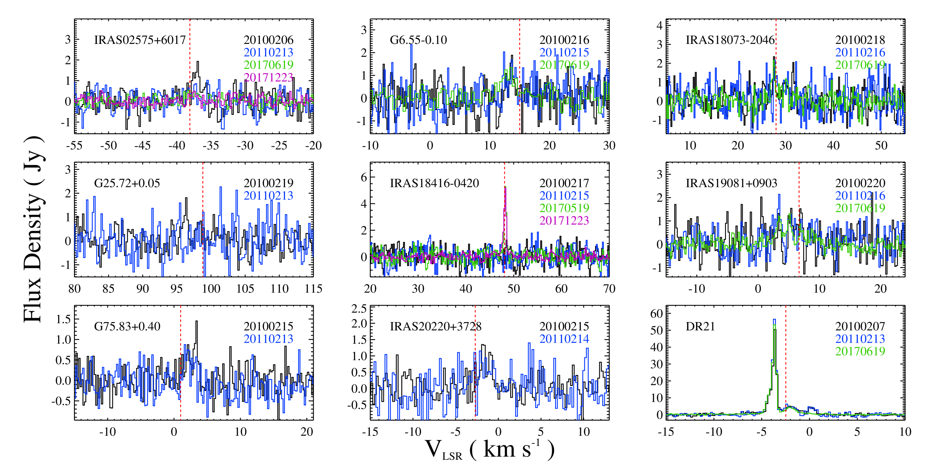
Figure 3: Spectra of only the CH₃OH maser-detected sources. Same symbols as in Figure 1.

Figures 1 and 3 exhibit the detected CH₃OH maser spectra. CH₃OH maser sources usually have one or two spectral features. These masers tend to show much simpler line profiles and narrower line-widths than H₂O masers. They always have very similar velocities to those of the natal dense cores. We also detected quasi-thermal CH₃OH emission features along with the maser emission toward some sources: G10.30$-$0.15, G10.47$+$0.03, G12.21$-$0.10, G31.41$+$0.31, IRAS18456$-$0129, W51d, and IRAS19410$+$2336. These sources will be discussed in § 4.2. The line parameters of the detected H₂O and CH₃OH masers are tabulated in Tables 3 and 4, respectively.

Figure 4 compares the peak flux densities of the detected H₂O and CH₃OH masers. In this comparison, we used the first-epoch data for the sources with the coordinate offsets $<\,10^{\prime\prime}$ and the third- or fourth-epoch data for the others with larger offsets. The H₂O masers have higher flux densities than the CH₃OH masers in the vast majority of the sources with both masers. The median values of H₂O and CH₃OH masers are $\sim$ 19 Jy and $\sim$  5 Jy, respectively, which are marked in the black dashed lines. The majority of H₂O maser sources have higher peak flux densities than 10 Jy, while most CH₃OH maser sources have lower values than that. In addition, the distribution range is much wider for H₂O masers than for CH₃OH masers. Some of the sources, however, show higher peak fluxes of CH₃OH masers than those of H₂O masers: G5.89$-$0.39, G10.30$-$0.15, IRAS18162$-$2048, G23.71$+$0.17, G27.28$+$0.15, G30.54$+$0.02, IRAS18469$-$0132, G33.92$+$0.11, G35.05$-$0.52, G42.42$-$0.27, and IRAS22176$+$2048. Three of them (18162$-$2048, G23.71$+$0.17, G35.05$-$0.52, and IRAS22176$+$6303) have 2$-$16 times stronger CH₃OH maser emission than H₂O maser emission.

Figure 5 displays the velocity range distributions of the detected H₂O and CH₃OH masers. Here $V_{\rm low}$ and $V_{\rm high}$ are the lowest and highest velocities of the velocity range of each source (Table 3). These velocities were measured at the 3$\sigma$ noise level. All the CH₃OH maser sources show smaller velocity ranges than 10 km s^-1, and the vast majority (74%) of them have velocity ranges $<$ 5 km s^-1. On the other hand, about (60%) of the H₂O maser sources have larger velocity ranges than 10 km s^-1. Moreover, five sources have velocity ranges greater than 100 km s^-1, and many of their maser lines are extremely shifted and variable as seen in the upper panel of Figure 1 and Table 3: G30.54$+$0.02 (111.3 km s^-1 in 2011), G34.26$+$0.15 (114.3 km s^-1 in 2010), IRAS19095$+$0930 (117.8 km s^-1 in 2010), W51d (223.4 $-$ 300.6  km s^-1 in 2010, 2011, and 2017), IRAS20081$+$3122 (115.9 and 104.1 km s^-1 in 2010 and 2011). W51d shows the largest velocity range in each of the three observed epochs: 223.4 km s^-1 in 2010, 250.3 km s^-1 in 2011, 300.6 km s^-1 in 2017 June. The W51d is located together with another UCHii (W51d1) and a hot core (W51-North) within a few arcseconds in the W51 IRS2 complex (Zapata et al., 2009; Goddi et al., 2015). Due to our bigger beam size than the complex region, there is an uncertainty to clarify the origin of the extremely-shifted H₂O maser features.

3.2 Variability of Detected H₂O and 44 GHz CH₃OH Masers

As seen in Figures 1 and 2, H₂O masers generally show significant variations in the line intensity, profile, and velocity over the one-year time interval of our observations. It is well known that H₂O masers considerably vary on timescales as short as a few weeks (e.g., Wilking et al. 1994; Claussen et al. 1996; Furuya et al. 2001, 2003; Bae et al. 2011). For instance, no H₂O maser was detected toward IRAS19410$+$2336 in 2010, but bright four maser lines, with peak fluxes of 16.2 $-$ 48.7 Jy, appeared at velocities between 15.4 and 28.1 km s^-1 in 2011. IRAS20255$+$3712 showed an opposite case that bright three H₂O maser lines immensely weakened (the peak line intensity dropped from 67.1 to 3.1 Jy) or disappeared from 2010 to 2011. We also found such variations over about six-month time interval toward some of the observed sources in 2017 June and December. For example, one of red- or blueshifted lines of IRAS18456$-$0129 and G43.18$-$0.52 changed by $\sim$4 times in the peak flux. In the case of IRAS05393$-$0156, the detected maser lines have different velocities between the third and fourth epochs. Goddi et al. (2007) suggested that such high variability of H₂O maser emission can be caused by outflows or shocks passing through the emitting region.

In contrast, 44 GHz CH₃OH masers rarely show such variability (see Figures 1 and 3). For instance, G5.89$-$0.39 exhibited the same spectra in the first and second epochs. Furthermore, when the spectra are compared with the one obtained by Bachiller et al. (1990), no significant difference is found between them. However, there are some sources where noticeable variations in the line intensity are observed, i.e., IRAS06058$+$2138, G19.61$-$0.23, IRAS19598$+$3324. For example, G19.61$-$0.23 was found to consist of two CH₃OH maser lines at 41.2 km s^-1 (19.0 Jy) and 46.1 km s^-1 (3.8 Jy) in 2010, but only a single line was detected with about half the peak flux density, 8.2 Jy at 40.9 km s^-1 in 2011. The two CH₃OH lines detected in 2010 were observed in 2017 June, with a very similar profile despite its positional offset of 11^′′. Bachiller et al. (1990) detected one maser line with a peak flux density of $\sim$24 Jy at 41.4 km s^-1 toward this source at the same position. For comparison, 6.7 GHz Class II CH₃OH masers appear to be considerably more variable (e.g., Goedhart et al. 2004; Durjasz et al. 2019). They show even periodic variations in a few tens of sources (e.g., Sugiyama et al. 2018; Olech et al. 2019).

Figure 6 plots the peak velocity differences between the first and second epochs against the peak velocity of the first epoch for the sources with positional offsets $<10^{\prime\prime}$, and between the third and fourth epochs for the sources with offsets $>20^{\prime\prime}$. The velocity differences are invariably less than 10 km s^-1 for the CH₃OH masers. The standard deviation ($\sigma$) is 1.2 km s^-1 for all the sources, and it reduces to 0.6 km s^-1 without taking into account a large variable source, G31.41$+$0.31, with a velocity difference of 6.1 km s^-1. It is worth noting that in G31.41$+$0.31 the difference between the two peak fluxes of the first and second epochs (0.4 Jy) is smaller than the rms noise level, $\sim$0.6 Jy (Table 4). The small standard deviation indicates little variability of the CH₃OH peak velocities over six-month or one-year time intervals. On the other hand, the H₂O masers show much larger variations in the peak velocity. The standard deviations ($\sigma$) are 9.0 km s^-1 for all the sources and 5.3 km s^-1 after excluding G23.96$+$0.15, which shows a velocity change of 51 km s^-1. Genzel & Downes (1977) and Churchwell et al. (1990) detected H₂O maser emission around the systemic velocity of 79.6 km s^-1 toward G23.96$+$0.15. We also detected one maser line at a velocity of 82.4 km s^-1 in 2011 but found only new high-velocity maser line at a velocity of 31.6 km s^-1 in 2010. Outflow activities of the same young stellar objects (YSOs) can cause these high variations in the peak velocity, although we cannot exclude the possibility that the detected maser lines in different epochs are associated with distinct YSOs within our beam at 22 GHz. In order to address this issue, high-resolution observations with interferometers are required. Despite much larger variations on the whole, 57% (31/54) of the H₂O maser sources show smaller variations than 2 km s^-1. Breen et al. (2010a) also reported that a similar fraction (62%) of their 207 H₂O maser sources showed small velocity changes within $\pm$ 2 km s^-1 for about nine-month time interval. These results suggest that for each of H₂O and CH₃OH masers the same emitting regions continuedly generate bright spectral features in the majority of the maser sources.

4 Notes on some individual sources

4.1 High-velocity H₂O Maser Sources

Twenty-four of the 74 H₂O maser-detected sources have maser lines shifted by more than 30 km s^-1 with respect to the systemic velocities (Table 5). Thirteen of them show extremely high-velocity ($>$50 km s^-1) components. Out of the 24 sources, 15 (62%) have only blue-shifted high-velocity components, five (21%) have both blue- and red-shifted ones, and four (17%) have only red-shifted ones. In five sources the high-velocity components are the strongest lines: IRAS18162$-$2048, G23.96$+$0.15, G30.54$+$0.02, IRAS18534$+$0218, G42.90$+$0.57 (Figures 1 & 2). They are all blue-shifted except for G30.54$+$0.02 in the first epoch. As mentioned earlier, H₂O masers are known to trace the accretion disks and/or inner jets/outflows of YSOs (e.g., Torrelles et al. 1997; Goddi et al. 2011; Burns et al. 2015). Since it is very difficult to expect such high-velocity components in accretion disks, they are very likely to originate from jets/outflows. The measured radial velocity depends on the inclination angle ($\theta$) between the jet/outflow axis and the line of sight as cos $\theta$. Thus we cannot exclude the possibility that H₂O maser sources with lower relative velocities can also be related to jets/outflows with large inclination angles. Table 5 lists the 24 high-velocity H₂O maser sources. In the table and afterwards, HV and EHV mean high-velocity (30$-$50 km s^-1) and extremely high-velocity ($>$ 50 km s^-1) H₂O maser lines, respectively.

4.1.1 G8.67$-$0.36

G8.67$-$0.36 shows blue-shifted HV and EHV components with respect to the systemic velocity (35.3 km s^-1) in the first and second epochs, respectively (Figure 1). The EHV component at a velocity of $-$23.2 km s^-1 is detected in this study for the first time, while the HV component at a velocity of $-$4.3 km s^-1 has been reported by previous single-dish and VLA surveys (Forster & Caswell, 1989; Churchwell et al., 1990; Hofner & Churchwell, 1996). There is another massive YSO (G8.68$-$0.37) close to G8.67$-$0.36, but it is located about 1^′ away and has a systemic velocity of $+$37.2 km s^-1 (Longmore et al., 2011). It is unclear whether G8.68$-$0.37 is associated with H₂O maser, although Valdettaro et al. (2001) detected one maser line at 33.2 km s^-1 toward a midpoint between the two objects using the Medicina 32 m telescope with a beam size (FWHM) of 1.9^′. Thus the HV and EHV components are likely associated with jets/outflows from G8.67$-$0.36.

4.1.2 IRAS18162$-$2048

In the 2010 and 2011 epochs, IRAS18162$-$2048 (also known as G10.8841$-$2.592, HH 80$-$81, or GGD 27) shows strong maser lines around a velocity of $-$80 km s^-1, which are EHV blueshifted components with respect to the systemic velocity (12.2 km s^-1) (Figure 1). These EHV components between velocities of $-$90 and $-$40 km s^-1 have been reported by several previous surveys (Gomez et al., 1995; Codella et al., 1996; Martí et al., 1999; Furuya et al., 2003; Kurtz & Hofner, 2005). Other maser lines around the systemic velocity have also been reported by Furuya et al. (2003) and Kurtz & Hofner (2005), although none of those components was detected in our observations. According to the VLA observations of Gomez et al. (1995) and Kurtz & Hofner (2005), the EHV blueshifted components are located about 7^′′ northeast of the UCHii and thermal radio jet, and thus we cannot exclude the possibility that they may be related to a separate YSO.

4.1.3 G30.54$+$0.02

G30.54$+$0.02 shows only redshifted EHV lines at a velocity of $\sim$102 km s^-1 in 2010 (Figure 1). The EHV lines are shifted from the systemic velocity (48.0 km s^-1) by $\sim$54 km s^-1. The redshifted components disappeared in 2011, and new weak lines appeared between $-$66 and $-$33 km s^-1 and near the systemic velocity. Urquhart et al. (2011) also detected multiple maser lines between $-$40 and +70 km s^-1 using the Green Bank 100 m telescope (FWHM=30$\arcsec$) in a similar period (from 2009 Nov 25 to 2010 Dec 10). Hence the blue- and red-shifted EHV components seem to be very variable. There is no previous report about the redshifted EHV components.

4.1.4 IRAS20081$+$3122

IRAS20081$-$3122 (ON 1) shows a bunch of maser lines from $-$70 to $+$60 km s^-1, including blueshifted HV/EHV and redshifted HV components, in 2010 and 2011 (Figure 1). The blueshifted components are stronger than the redshifted ones. According to the H₂O maser monitoring result of Felli et al. (2007) toward this object for two decades (from 1987 March to 2007 February), maser lines around the systemic velocity (11.6 km s^-1) were usually the strongest, and blue- and redshifted HV/EHV lines were more frequently variable.

4.1.5 G75.78$+$0.34

G75.78$+$0.34 (ON 2) shows multiple maser lines between $-$25 and $+$20 km s^-1 in 2010 and 2011 (Figure 1). We detected a weak redshifted HV component at a velocity of $\sim$44.5 km s^-1 only in 2010. The HV line has not been detected either in the H₂O maser monitoring observations of Lekht et al. (2006) from 1995 to 2004 or in the VLA observation of Hofner & Churchwell (1996) due to their short velocity coverages. In the VLA image of Hofner & Churchwell (1996) a cluster of H₂O maser features with velocities between $-$20 and $+$15 km s^-1 are located $\sim 2\arcsec$ from the front of this cometary UCHii.

4.2 44 GHz CH₃OH Quasi-thermal Emission Sources

As mentioned in § 3.1, the detected 44 GHz CH₃OH maser lines usually have line-widths $\lesssim$1 km s^-1, much smaller than typical molecular line-widths, and they mostly have narrower widths than H₂O maser lines in high-mass star-forming regions. However, broad CH₃OH line wings are detected toward 7 sources with our sensitivity: G5.89$-$0.39, G10.30$-$0.15, G10.47$+$0.03, G12.21$-$0.10, G31.41$+$0.31, IRAS06058+2138, IRAS18456$-$0129, W51d, IRAS19410+2336. These features seem to be quasi-thermal emission rather than maser emission.

Several previous surveys of Class I CH₃OH masers have reported the detection of quasi-thermal emission accompanying maser emission (Bachiller et al., 1990; Haschick et al., 1990; Slysh et al., 1994; Mehringer & Menten, 1997; Pratap et al., 2008; Kalenskii et al., 2010; Kim et al., 2018a). Haschick et al. (1990) detected quasi-thermal emission from a few sources, including Orion-KL and Sgr A, among a half of 50 galactic star-forming regions. Also, Pratap et al. (2008) detected 36 GHz (4${}_{-1}-$3₀ E) CH₃OH  quasi-thermal emission from NGC 7538, and Kalenskii et al. (2010) found quasi-thermal CH₃OH emission at 36, 44, and/or 95 GHz frequencies toward some low-mass YSOs.

5 DISCUSSION

5.1 Detection Rates

We detected 22 GHz H₂O and 44 GHz CH₃OH maser emission toward 72% and 53% of the observed 103 UCHiis, respectively. These detection rates are determined from the combined result of all epochs and are mostly higher than those of each epoch, e.g., 62% and 40% in the first epoch, due to time variability of maser emission (Table 2). For comparison, we investigate the detection of 6.7 GHz Class II CH₃OH maser emission toward the sources in our sample from the literature (Xu et al., 2003; Pandian et al., 2007; Caswell et al., 2010; Green et al., 2010, 2012; Szymczak et al., 2012; Hou & Han, 2014; Breen et al., 2015; Hu et al., 2016). At least 34% (35) of them seem to be related to the maser emission, assuming a matching radius of 5^′′ (see Table 1). Eighty sources in our sample were covered by the Methanol Multibeam (MMB) survey (Green et al., 2009) using the Parks 64 m telescope (Caswell et al., 2010; Green et al., 2010, 2012; Breen et al., 2015). The detection rate is estimated to be 30% (24/80), considering 24 out of the 35 sources are distributed in the MMB survey area (see Table 1).

To understand the relationship between maser activity and central objects, we investigate the H₂O maser detection rates of massive star-forming regions in different evolutionary stages, including infrared dark cloud cores (IRDCs), HMPOs, and UCHiis. The H₂O maser detection rate of UCHiis in this survey is significantly higher than the detection rates of HMPOs (42%, Sridharan et al. 2002; 52%, Szymczak et al. 2005; 52%, Urquhart et al. 2011; 51%, Kang et al. 2015; 45%, Kim et al. 2018a) and IRDCs (12%, Wang et al. 2006; 35%, Chambers et al. 2009) although these surveys were done with similar or better sensitivities of $\sim$0.1$-$0.5 Jy. This suggests that the detection rate of H₂O maser increases with the evolution of the central objects. This trend is in contrast with the survey results toward low- and intermediate-mass star-forming regions in which the detection rate rapidly decreases as the central objects evolve. Furuya et al. (2001) detected H₂O maser emission in 40% of Class 0, 4% of Class I, and none of Class II objects in low-mass star-forming regions. Bae et al. (2011) also found a similar trend toward intermediate-mass YSOs: 50% for Class 0, 21% for Class I objects, 3% of Herbig Ae/Be stars. This difference might be caused by different environments surrounding low- and high-mass YSOs, as Bae et al. (2011) suggested. The circumstellar materials are mostly dispersed by protostellar outflows around low- and intermediate YSOs in later evolutionary stages. On the other hand, UCHiis are still deeply embedded in the parental molecular clouds due to their faster evolution and much larger amount of ambient matter although the ionizing stars have already reached the main-sequence stage.

The situation is very similar for the 44 GHz CH₃OH maser detection rate. Our value for UCHiis is considerably higher than the rate (31$\pm$5%) toward HMPOs reported by the single-dish survey of Fontani et al. (2010) with a comparable sensitivity of $\sim$0.6 Jy at velocity resolution of $\sim$0.2 km s^-1 to this survey. Their sample consists of two groups: low and high sources. The high sources satisfy the $IRAS$ color criteria of Wood & Churchwell (1989b) for UCHiis, i.e., UCHii candidates without detectable radio continuum emission in single-dish observations, and are believed to be more evolved than the low sources. They estimated the detection rates for the two groups separately and found that the rate for the high sources (48$\pm$8%) is almost three times higher than that of the low sources (17$\pm$5%). The former rate is in a good agreement with ours. Kang et al. (2015) and Kim et al. (2018a) also obtained lower detection rates of 32% and 28%, respectively, with almost the same sensitivities at the same velocity resolution as this survey. On the contrary, the detection rate of 44 GHz CH₃OH maser emission decreases with the evolution of the central objects in intermediate-mass star-forming regions: 36% for Class 0, 21% for Class I, 1% for HAeBe objects (Bae et al., 2011). This difference can also be understood by the same explanations as for the H₂O maser detection rate.

Taking into account low angular resolutions of this survey, we cannot exclude the possibility that the detected masers may be associated with nearby YSOs rather than target UCHiis. However, previous high-resolution VLA observations showed strong angular correlations between the two maser species and UCHiis (Hofner & Churchwell, 1996; Kurtz et al., 2004; Gómez et al., 2010; Gómez-Ruiz et al., 2016). These studies found that H₂O maser spots are located within $\sim$0.1 pc of the UCHiis, and 44 GHz CH₃OH maser spots are separated by $<$0.5 pc with a mean separation of 0.2 pc. Gómez-Ruiz et al. (2016) found more than twice higher detection rate (63%) for the $high$ sources than that (27%) for $low$ sources in their VLA observations of 44 GHz CH₃OH masers toward the sample of Fontani et al. (2010). As mentioned in § 1, these two maser species are known to be closely related to protostellar outflows although they trace different parts of the outflows. According to Shepherd & Churchwell (1996), the vast majority of UCHiis (90%, of 94 sources) still have bipolar outflows as in HMPOs (Sridharan et al., 2002; Zhang et al., 2005; Kim & Kurtz, 2006). Therefore, it is not surprising that a significant fraction of UCHiis are associated with H₂O and/or 44 GHz CH₃OH maser emission. Moreover, a few high-resolution observations with the Austrailia Telescope Compact Array (ATCA) provided a hint that 44 GHz CH₃OH masers can be generated in the shocked regions by the expansion of UCHiis (Voronkov et al. 2010, 2014; see also Kurtz et al. 2004; Gómez-Ruiz et al. 2016).

5.2 Relative Velocities of Masers

Figures 7 and 8 show the relative velocities of H₂O and 44 GHz CH₃OH masers versus the systemic velocities, respectively. In all analyses in this section, we use the 2010 data for the sources with coordinate offsets $<$10^′′ and the 2017 data for the other sources. The relative velocities of H₂O maser lines span from $-$130 to 170 km s^-1, including W51d that is not plotted in Figures 7 for clarity. The mean value and standard deviation ($\sigma$) of the relative velocities of all components are $-$5.2 and 32.4 km s^-1, respectively. The vast majority (88%) of the peak maser velocities, marked by open circles, are concentrated within the relative velocity range of $\pm$ 20 km s^-1. The mean and standard deviation ($\sigma$) of the peak relative velocities are $-$4.4 and 19.2 km s^-1, respectively. This relatively good agreement between the peak H₂O maser and systemic velocities corresponds with the results of some previous surveys (e.g., $-$4.5 km s^-1, Kurtz & Hofner 2005; $-$3.8 km s^-1, Urquhart et al. 2011). Low- and high-velocity H₂O maser components are considered to be produced by slow wide-angle outflows and fast well-collimated jets, respectively (Gwinn et al., 1992; Torrelles et al., 2011; Goddi et al., 2011). According to theoretical models, H₂O masers are formed in warm ($\sim$ 500 K) and very dense ($\sim$ 10⁹ cm^-3) shocked gas behind fast-velocity ($>$ 50 km s^-1) dissociative shocks (J$-$type) or slow-velocity ($<$ 50 km s^-1) non-dissociative shocks (C$-$type) (Elitzur et al., 1989; Kaufman & Neufeld, 1996). H₂O masers can, therefore, have a wide range of relative velocities because of being accelerated by various velocity outflows.

In contrast to H₂O masers, the relative velocities of 44 GHz CH₃OH maser lines never exceed $\pm$10 km s^-1 as seen in Figure 8. This result supports that CH₃OH molecules can survive only in slow shocks below 10 km s^-1 but are easily destroyed by fast-moving shocks over 10 km s^-1 (e.g., Garay et al. 2002). The peak velocity components of 44 GHz CH₃OH masers are also located in a narrow range of relative velocities. They are mostly (79%) located within $\pm$ 2 km s^-1 with respect to the systemic velocity. This excellent agreement between the peak 44 GHz CH₃OH maser and systemic velocities is consistent with the fact that Class I CH₃OH masers are located in the interacting regions between outflows and the ambient gas (Plambeck & Menten, 1990; Kurtz et al., 2004). Theoretical models and high-resolution observations have revealed that Class I CH₃OH masers originate from cooler and less dense gas (temperature of $\sim$100 K and densities $\sim$ 10⁵ cm^-3) than H₂O masers (Cragg et al., 1992). Such condition is found in post-shock regions farther from a central object (0.2$-$0.5 pc; Kurtz et al. 2004; Gómez et al. 2010) than that typically found for H₂O masers ($\sim$ 0.1 pc; Hofner & Churchwell 1996). However, it should be noted that in a few sources Class I CH₃OH masers appear to be associated with the expansion of Hii regions (Voronkov et al., 2010; Araya et al., 2008) or by accretion shocks (Kurtz et al., 2004). Although H₂O and 44 GHz CH₃OH masers are commonly excited by collisional pumping by shocks from jets/outflows, there is a significant difference between the velocity distributions of the two maser species. This may indicate that H₂O and CH₃OH masers are generated from different parts of the outflows and are sensitive to different physical conditions in the vicinity of (proto)stars.

5.3 Environmental Conditions of Masers

The total isotropic luminosities of H₂O and CH₃OH masers ($L_{\rm{H_{2}O}}$ and $L_{\rm{CH_{3}OH}}$) can be calculated by the following equations:

$$L_{\rm{H_{2}O}} = 4\pi d^{2}{\frac{\nu}{c}}\int{F_{\nu}}\,dv$$ (1)

$$= 2.32\times 10^{-8}L_{\odot}\bigg{(}\frac{d}{1~{}\rm{kpc}}\bigg{)}^{2}\bigg{(}\frac{\int{S_{\nu}}\,dv}{1\,\rm{Jy\,km\,s}^{-1}}\bigg{)}\bigg{(}\frac{\eta_{a}}{0.72}\bigg{)}^{-1},$$

and

$$L_{\rm{CH_{3}OH}}=4.60\times 10^{-8}L_{\odot}\bigg{(}\frac{d}{1~{}\rm{kpc}}\bigg{)}^{2}\bigg{(}\frac{\int{S_{\nu}}\,dv}{1\,\rm{Jy\,km\,s}^{-1}}\bigg{)}\bigg{(}\frac{\eta_{a}}{0.69}\bigg{)}^{-1}.$$ (2)

Here $d$ is the distance to the source, $\nu$ is the observing frequency, $\int{S_{\nu}}\,dv$ is the integrated flux density, and $\eta_{a}$ is the aperture efficiency of the telescope. We adopt the kinematic distances from WC89a and KWC94 and a few other references, as noted in Table 6. In a case where the maser emission consists of multiple lines, the sum of the individual components is used for $\int{S_{\nu}}\,dv$ as in some previous studies (e.g., Furuya et al. 2003; Bae et al. 2011). The estimated maser luminosities of H₂O and CH₃OH masers are given in columns (8) and (9) of Table 6, respectively. The table also provides the physical parameters of UCHiis and their parental clumps.

5.3.1 Comparison of Bolometric Luminosity and Maser Luminosity

Figure 9 shows $L_{\rm{H_{2}O}}$ and $L_{\rm{CH_{3}OH}}$ against the bolometric luminosity of the central star ($L_{\rm bol}$). The relation for H₂O masers by linear least-squares fitting is $L_{\rm{H_{2}O}}=1.01\times 10^{-11}(L_{\rm{bol}})^{1.17}$ with a correlation coefficient ($\rho$) of 0.66. The fitted result for 44 GHz CH₃OH masers is $L_{\rm{CH_{3}OH}}=6.70\times 10^{-10}(L_{\rm{bol}})^{0.76}$ with $\rho=$0.52. The former and latter relations are shown by dotted lines in the upper and lower panels, respectively. Both $L_{\rm{H_{2}O}}$ and $L_{\rm{CH_{3}OH}}$ tend to increase with $L_{\rm bol}$. The correlations get significantly stronger when the data points of the low- and intermediate-mass regimes are added to the UCHiis. The newly fitted relations are $L_{\rm{H_{2}O}}=3.56\times 10^{-9}(L_{\rm{bol}})^{0.71}$ with $\rho=0.89$, and $L_{\rm{CH_{3}OH}}=7.61\times 10^{-9}(L_{\rm{bol}})^{0.56}$ with $\rho=0.80$. They are shown by solid lines in both panels. Here the data of LMYSOs are taken from Furuya et al. (2003) for H₂O masers and Kalenskii et al. (2010) for CH₃OH masers, and the data of IMYSOs are from Bae et al. (2011) for both maser species. Bae et al. (2011) also did similar analyses by combining their data of IMYSOs with the preliminary results of this study and obtained a little bit higher slopes for both relations, 0.84 and 0.73. This is mainly because they derived $L_{\rm bol}$ of UCHiis  using the VLA radio continuum data rather than the $IRAS$ data as in this study. For a given UCHii, the $L_{\rm bol}$ from the radio continuum data is always smaller than that from the $IRAS$ data due to the absorption of part of UV photons by dust inside the UCHii (Wood & Churchwell, 1989a; Kurtz et al., 1994), and the contributions of low/intermediate-mass star clusters in the region (Kim et al., 2018b). These results demonstrate that more luminous (and massive) stars are likely to generate more luminous H₂O and CH₃OH masers.

Figure 10 shows the comparison of the two maser luminosities. The dotted line is the best fit of only UCHiis while the solid line is the fit to all the data points including LMYSOs and IMYSOs. The former is $L_{\rm{CH_{3}OH}}=8.75\times 10^{-3}(L_{\rm{H_{2}O}})^{0.45}$ with $\rho=0.54$, and the latter is $L_{\rm{CH_{3}OH}}=2.42\times 10^{-3}(L_{\rm{H_{2}O}})^{0.57}$ with $\rho=0.70$. For all the data points, a good correlation is found between the two maser luminosities. This strongly supports the previous suggestion that the two masers are both collisionally pumped by outflows (e.g., Kurtz et al. 2004). Indeed, Felli et al. (1992) found in 56 CO outflow sources that $L_{\rm{H_{2}O}}$ correlates with the mechanical luminosity of the outflow, which is, in turn, proportional to the far-infrared luminosity. Gan et al. (2013) detected 95 GHz class I CH₃OH maser emission toward 62 CO outflow sources and found significant correlations between the maser luminosity and the outflow properties such as mass, momentum, and mechanical energy. Kim et al. (2018a) showed from a simultaneous surveys of 44 and 95 GHz CH₃OH masers that the two maser transitions have tight correlations in the line velocity, flux density, and profile (see also Kang et al. 2015).

5.3.2 Comparison of Radio Continuum Luminosity and Maser Luminosity

Figure 11 plots $L_{\rm{H_{2}O}}$ and $L_{\rm{CH_{3}OH}}$ versus the radio continuum luminosity at 2 cm ($L_{\rm{2\,\mbox{cm}}}$). The linear least-squares fittings yield $L_{\rm{H_{2}O}}=6.65\times 10^{-11}(L_{\rm 2\,{\mbox{cm}}})^{0.54}$ with $\rho=0.57$ and $L_{\rm{CH_{3}OH}}=7.71\times 10^{-12}(L_{2\,{\mbox{cm}}})^{0.55}$ with $\rho=0.68$. The $L_{\rm{2\,\mbox{cm}}}$ also tends to increase with $L_{\rm{H_{2}O}}$ and $L_{\rm{CH_{3}OH}}$ like $L_{\rm{bol}}$. The $L_{\rm{CH_{3}OH}}$ shows a better correlation with $L_{\rm{2\,\mbox{cm}}}$ than $L_{\rm{H_{2}O}}$. Figure 12 shows a comparison between the $L_{\rm{H_{2}O}}$ and 6 cm radio continuum luminosity ($L_{\rm{6\mbox{cm}}}$) of LMYSOs (Furuya et al., 2003) and UCHiis. The dotted line indicates the fitted relation of LMYSOs. On the other hand, the solid line is a leaner-fitting on both LMYSOs and UCHiis, $L_{\rm{H_{2}O}}=1.42\times 10^{-11}(L_{\rm 6\,{\mbox{cm}}})^{0.60}$ with $\rho=0.84$. This seems to be the best correlation between the maser and radio continuum luminosities. Here it should be noted that LMYSOs and UCHiis have different origins of radio continuum emission. The radio continuum emission of LMYSOs originates from ionized jets or ionized gas regions by a neutral jet-induced shock (Rodriguez, 1989; Meehan et al., 1998), while the radio continuum emission of massive star-forming regions mostly emanates from Hii regions. Nonetheless, their $L_{\rm 6cm}$ have excellent correlations with $L_{\rm{H_{2}O}}$. The reason is likely that the maser luminosity and radio continuum luminosity are both influenced by the bolometric luminosity of the central (proto)star. In fact, the radio continuum luminosity is known to correlate with the bolometric luminosity for LMYSOs (Anglada, 1995; Claussen et al., 1996; Meehan et al., 1998).

5.3.3 Comparison of Molecular Clump Properties and Maser Luminosity

Figure 13 shows comparisons of $L_{\rm{H_{2}O}}$ and $L_{\rm{CH_{3}OH}}$ versus 850 $\mu$m continuum luminosity ($L_{\rm{850\mu m}}$). The submillimeter continuum emission emitted from cold dust indirectly provides mass information of molecular clumps and cores (Thompson et al., 2006; Schuller et al., 2009). The fitted results are $L_{\rm{H_{2}O}}=1.95\times 10^{-11}(L_{\rm 850\mu m})^{0.63}$ with $\rho=0.35$ and $L_{\rm{CH_{3}OH}}=6.48\times 10^{-18}(L_{\rm 850\mu m})^{1.22}$ with $\rho=0.77$. While the $L_{\rm{H_{2}O}}$ is weakly correlated with $L_{\rm{850\mu m}}$, the $L_{\rm{CH_{3}OH}}$ strongly correlates with it. Kim et al. (2018a) also investigated the correlations of the two maser luminosities with the host clump mass and reported significant correlations for both masers. de Villiers et al. (2014) showed that the outflow mass and mass-loss rate have clear correlations with the clump mass, and Urquhart et al. (2014) found that the bolometric luminosity tightly correlates with the clump mass. These correlations suggest that more massive clumps form more massive (and luminous) stars, which emit more energetic outflows that can generate stronger H₂O and class I CH₃OH masers.

5.4 Evolutionary Sequence for Masers in Massive Star Formation

One major question of the maser study is whether a maser species traces any specific evolutionary stage of massive star formation. As massive (proto)stars evolve, their strong radiation and powerful jets/outflows tremendously impact on the physical, chemical, and dynamical properties of the surrounding materials. The changing physical and chemical conditions in the circumstellar region can lead to the production of different maser species in different evolutionary phases. As mentioned earlier, H₂O, CH₃OH (Class I & Class II), and/or OH masers have been found to be associated with a number of massive star-forming regions in different stages. In many cases multiple different maser species have been detected toward the same object (e.g., Beuther et al. 2002). This indicates that there may be significant overlaps between different maser phases. Ellingsen (2006) found that Spitzer point sources with both Class I and Class II CH₃OH masers tend to have redder infrared colors than those with only Class II CH₃OH masers and argued that Class I CH₃OH masers may trace earlier evolutionary stages of massive star formation than Class II CH₃OH (and H₂O) masers. Ellingsen et al. (2007) later proposed an evolutionary sequence of different maser species in which H₂O masers primarily appear in the UCHii phase while Class I CH₃OH masers appear at earlier evolutionary stages and then mostly disappear as UCHiis develop (see also Breen et al. 2010b). However, the high association rates of both H₂O and 44 GHz Class I CH₃OH masers with the UCHii phase in this study appear to cast some doubt on the hypothesis. Furthermore, the increasing detection rate as a function of evolution also indicates that Class I CH₃OH masers preferentially trace the later stages of massive star formation.

Since massive stars usually form in cluster rather than in isolation, it is possible that the high detection rates we have found may result from outflows driven by other cluster members with lower masses. However, the correlation of maser luminosity with the bolometric and radio continuum luminosities would make this seem less likely (see Figures 9, 11, and 12). It is also possible that the high detection rates may be due to the contribution of nearby HMPOs producing outflows within the telescope beam. However, the possibility could be negligible, as we have discussed in § 5.1, according to positional coincidence between maser features and the ionized gas regions in previous high-resolution observations (Hofner & Churchwell, 1996; Kurtz et al., 2004; Voronkov et al., 2010, 2014) and the ubiquity of jets/outflows in UCHiis (Shepherd & Churchwell, 1996; Hatchell et al., 2001; Kurtz et al., 2004). In the recent VLA high-resolution observations of Gómez-Ruiz et al. (2016), the detection rate (54%, 13 of 24) of 44 GHz CH₃OH maser emission toward UCHii candidates was higher than that (38%, 16 of 42) toward HMPOs. This is consistent with the result of this survey even though the two surveys were carried out with very different angular resolutions. In addition, a few studies (Araya et al., 2008; Voronkov et al., 2010, 2014; Gómez-Ruiz et al., 2016) imply that Class I CH₃OH masers can be produced by the expansion of Hii regions, as well.

Our finding therefore appears to agree with the results obtained from several previous high-resolution studies but disagrees with the maser evolutionary sequence put forward by Ellingsen et al. (2007) and Breen et al. (2010b). One possible reason for this disagreement could be that their analyses were restricted to massive YSOs with Class II CH₃OH masers and did not include the later UCHii region stage and so were focused on a relatively small range of evolution. In contrast, we conducted a simultaneous H₂O and 44 GHz Class I CH₃OH masers toward a large sample of UCHiis and provide more reliable information of the UCHii phase in evolutionary sequence in terms of maser detection. All the results of the present and several previous studies strongly suggest that the occurrence periods of the two maser species are more closely overlapped with the UCHii phase than earlier evolutionary phases.

6 SUMMARY

We performed a multi-epoch simultaneous survey of 22 GHz H₂O and 44 GHz Class I CH₃OH masers toward 103 UCHiis. The main results are summarized as follows.

1. H₂O maser emission was detected in 74 (72%) sources and CH₃OH maser emission in 55 (53%) sources. These high detection rates suggest that the occurrence periods of both masers are significantly overlapped with the UCHii phase. This is not consistent with the previous suggestion that Class I CH₃OH masers fade out as UCHiis develop. By combining this with the results of some previous maser surveys towards IRDCs and HMPOs, furthermore, we found that the two detection rates may increase with the evolution of the central objects and peak in the UCHii phase. Among the detected sources, 3 H₂O and 27 CH₃OH maser sources are new detections. The WC89a sample show slightly higher detection rates for both masers than the KCW94 sample.

2. CH₃OH maser lines always have small ($<$10 km s^-1) relative velocities with respect to the ambient dense molecular gas, while H₂O maser lines usually have much larger relative velocities. We found a few tens of H₂O maser sources with high-velocity components. Twenty four sources have H₂O maser lines with relative velocities $>$30 km s^-1, and thirteen of them have H₂O maser lines with relative velocities $\geq$50 km s^-1. It is worth noting that the strongest maser lines have relative velocities $<$20 km s^-1 for the vast majority (88%) of the H₂O maser-detected sources.

3. H₂O masers generally have multiple velocity components with wide velocity ranges. They often show significant variations in the line shape, intensity, and velocity over six-months or one-year time intervals although the strongest maser lines of the individual sources mostly display small variations in velocity. In contrast, CH₃OH masers usually have one or two velocity components, and rarely exhibit significant variations in the line shape, intensity, or velocity for the same periods. This difference, together with the difference between the typical relative velocities of the two maser species, is very likely to arise from their different emitting regions.

4. The isotropic luminosities of both masers tend to increase with the bolometric luminosity of the central star. In the case of that data points of low- and intermediate-mass star-forming regions are added, they well correlate with the bolometric luminosity. The linear fitted relations $L_{\rm{H_{2}O}}=3.56\times 10^{-9}(L_{\rm bol})^{0.71}$ and $L_{\rm{CH_{3}OH}}=7.61\times 10^{-9}(L_{\rm bol})^{0.59}$. There is a quite good correlation between the two maser luminosities.

5. The two maser luminosities tend to increase with the radio continuum luminosity. The linear fitted relations are $L_{\rm{H_{2}O}}=6.65\times 10^{-11}(L_{\rm{2\,\mbox{cm}}})^{0.54}$ and $L_{\rm{CH_{3}OH}}=7.71\times 10^{-12}(L_{\rm{2\,\mbox{cm}}})^{0.55}$. The CH₃OH maser luminosity also shows a tight correlation with the 850 $\mu$m emission luminosity of the associated molecular clump. These correlations suggest that more massive clumps form more massive (and luminous) stars that can generate stronger H₂O and class I CH₃OH masers through more energetic outflows.

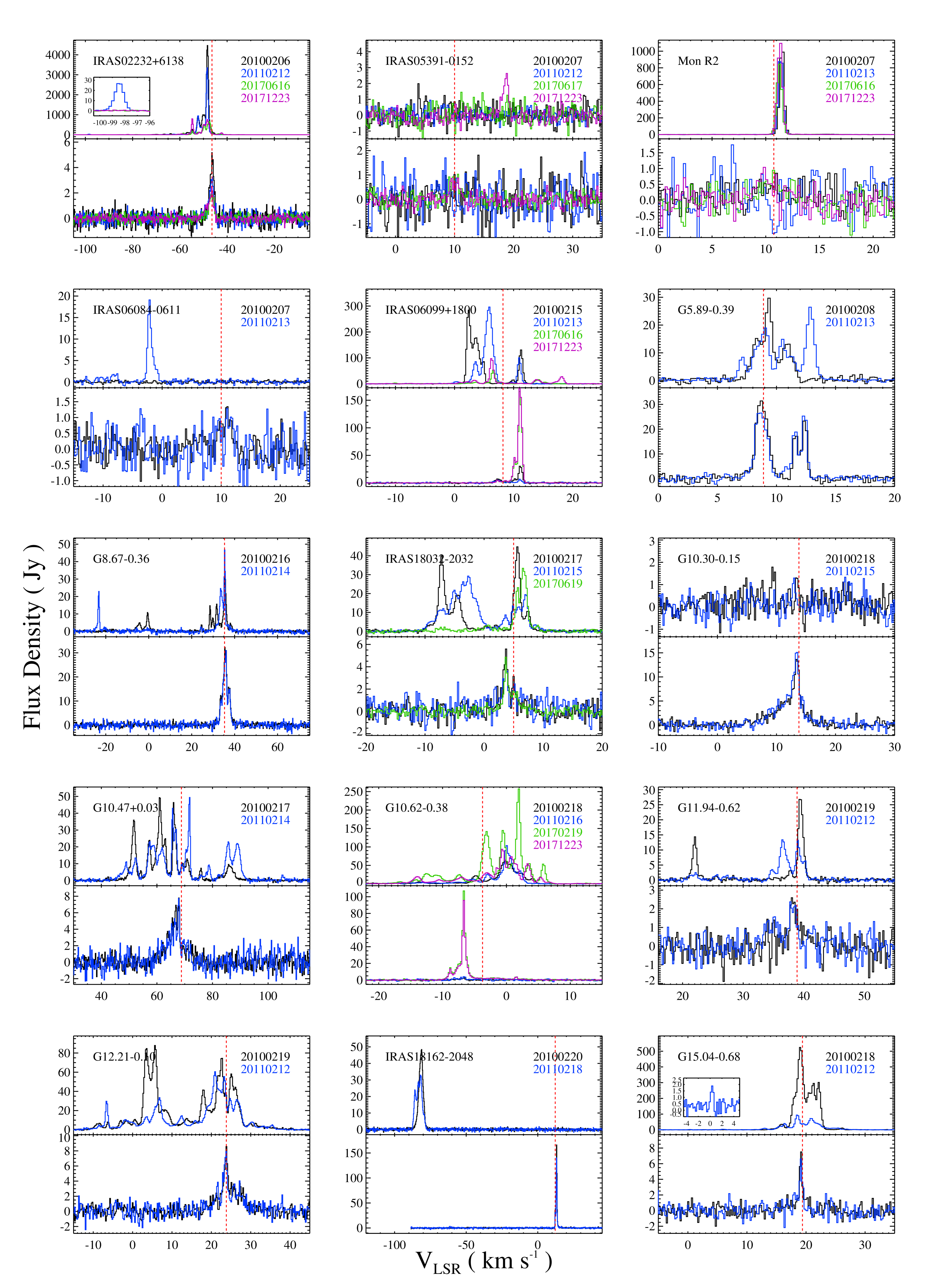
Figure 1: 22 GHz H₂O (upper panel) and 44 GHz CH₃OH (lower panel) maser spectra of the sources detected in both maser emission. Different colors indicate different observation epochs. In each panel, the source name is presented at the top-left corner and the observing dates are listed at the top-right corner. The vertical dotted line shows the systemic velocity. High-velocity H₂O maser lines are expanded in the insets.

Fig. 1.— Continued.

Fig. 1.— Continued.

Fig. 1.— Continued.

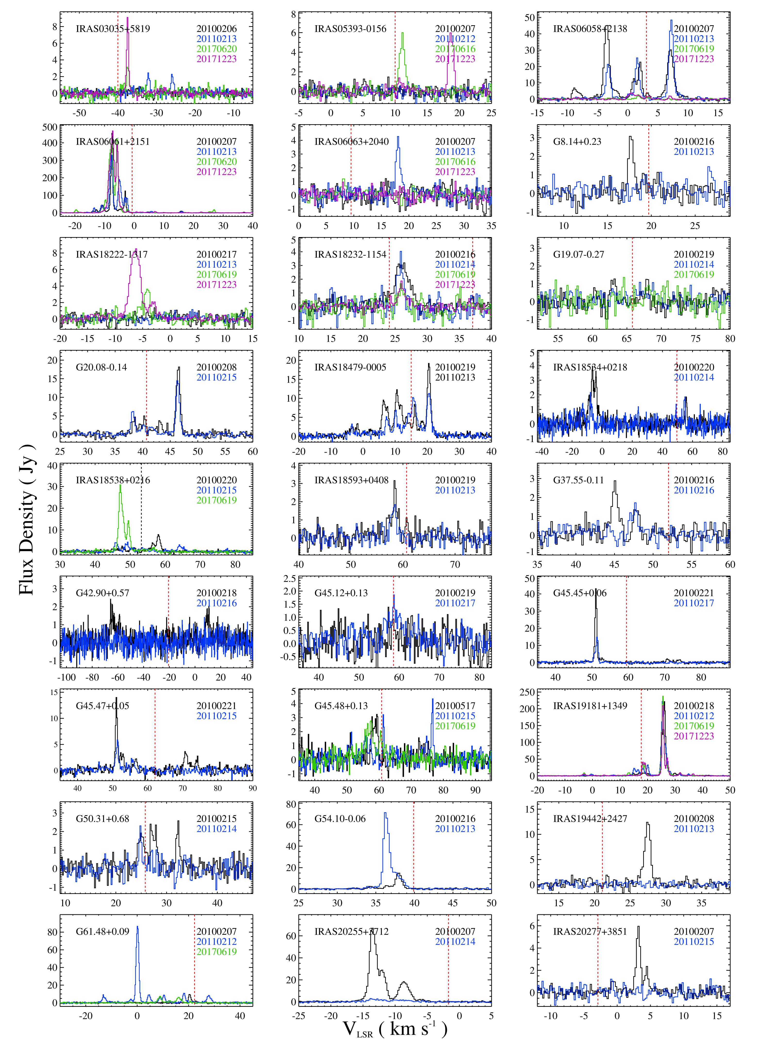
Figure 2: Spectra of only the H₂O maser-detected sources. Same symbols as in Figure 1.

Fig. 2 — Continued.

Figure 4: Histogram of the flux densities for (a) H₂O and (b) CH₃OH masers. The bin size is 0.5 dex. The vertical dashed line indicates median value of the flux densities of each maser species.

Figure 5: Histogram of the velocity ranges of (a) H₂O and (b) CH₃OH masers. The bin sizes are 10 km s^-1 and 0.5 km s^-1 for H₂O and CH₃OH masers, respectively. The vertical dashed line indicates median value of the velocity ranges for each maser species.

Figure 6: Peak velocity difference between the first and second or the third and fourth epochs versus the peak velocity of the first or the third epochs for (a) H₂O and (b) CH₃OH masers. G23.96$+$0.15 is not plotted in the upper panel because its velocity difference is in excess of the plot range (see details in the text).

Figure 7: Relative velocity of H₂O maser line versus systemic velocity. The first-epoch data are plotted for the sources with the coordinate offsets $<$10^′′ while the third- or fourth-epoch data are plotted for the other sources. Open circles indicate the strongest maser lines in the individual sources. All the line components of W51d are not plotted here because of its large velocity range, $-$130 to 170 km s^-1.

Figure 8: Relative velocity of CH₃OH maser line versus systemic velocity. Same symbols as in Figure 7.

Figure 9: Isotropic maser luminosity as a function of bolometric luminosity of the central star for (a) H₂O and (b) CH₃OH masers. Filled circles are WC89a sources while open circles are KCW94 sources. Open diamonds, open triangles, and open squares indicate IMYSOs in Class 0, Class I, and HAeBe stages, respectively (Bae et al., 2011). In (a), filled triangles and filled squares represent LMYSOs (Furuya et al., 2003). In (b), filled triangles indicate LMYSOs (Kalenskii et al., 2013). The dotted and solid lines are the best-fit relations for UCHiis and for all objects, respectively.

Figure 10: H₂O maser luminosity as a function of CH₃OH maser luminosity. The filled circles are WC89a sources while the open circles are KCW94 source. Diamonds, triangles, squares indicate the data points of IMYSOs in Class 0, Class I, and HAeBe stages from Bae et al. (2011), respectively. Filled squares are LMYSOs from Kalenskii et al. (2010). The dotted line shows the fitted relation of only UCHii data points, whereas the solid line represents the one of all data points (see the text for more details).

Figure 11: Isotropic maser luminosity as a function of 2 cm radio continuum luminosity for (a) H₂O and (b) CH₃OH masers. Filled circles are WC89a sources, and open circles are KCW94 sources.

Figure 12: Isotropic H₂O maser luminosity as a function of 6 cm radio continuum luminosity. Circles represent UCHiis, and filled triangles and squares show LMYSOs from Furuya et al. (2003)

Figure 13: Isotropic maser luminosity as a function of 850 ${\mu}$m luminosity for (a) H₂O and (b) CH₃OH masers. Filled circles are WC89a sources, while open circles are KCW94 sources. The solid lines show the best-fits to the data.

Table 1: Source Summary

Source	Ref.	R.A. (2000)	Dec. (2000)	Offset	Station	Observing	Maser detection		$\sigma_{\rm H_{2}O}$	$\sigma_{\rm CH_{3}OH}$	6.7 GHz	Other name
Name		(h m s)	(° ′ ″)	″		Date	H2O	CH3OH	(Jy)	(Jy)	Maser
(1)	(2)	(3)	(4)	(5)	(6)	(7)	(8)	(9)	(10)	(11)	(12)	(13)
IRAS02232$+$6138	2	02:27:01.0	$+$61:52:14	23	YS	2010 Feb 06	Y	Y	0.38	0.52		G133.947$+$1.064, W3OH
					YS	2011 Feb 12	Y	Y	1.15	0.37
		02:27:03.8	$+$61:52:25		YS	2017 Jun 16	Y	Y	0.49	0.24	Y∗
					YS	2017 Dec 23	Y	Y	0.35	0.20
IRAS02575$+$6017	2	03:01:32.3	$+$60:29:12	15	YS	2010 Feb 06	N	Ya	0.39	0.53		G138.295$+$1.555, W5E
					YS	2011 Feb 13	N	N	0.31	0.44
		03:01:34.3	$+$60:29:14		US	2017 Jun 19	N	N	0.29	0.21
					YS	2017 Dec 23	N	N	0.29	0.21
IRAS03035$+$5819	2	03:07:25.6	$+$58:30:52	15	YS	2010 Feb 06	N	N	0.30	0.42		G139.909$+$0.197, AFGL437
					YS	2011 Feb 13	Y	N	0.33	0.47
		03:07:23.7	$+$58:30:50		US	2017 Jun 20	Y	N	0.47	0.34
					YS	2017 Dec 23	Y	N	0.26	0.16
IRAS05391$-$0152	2	05:41:38.7	$-$01:51:19	143	YS	2010 Feb 07	N	N	0.56	0.64		$\cdots$
					YS	2011 Feb 12	N	N	0.39	0.64
		05:41:41.3	$-$01:53:37		YS	2017 Jun 17	N	Y	0.49	0.23
					YS	2017 Dec 23	Y	Y	0.35	0.25
IRAS05393$-$0156	2	05:41:49.5	$-$01:55:17	73	YS	2010 Feb 07	N	N	0.59	0.63		G206.543$-$16.347
					YS	2011 Feb 12	N	N	0.41	0.64
		05:41:45.7	$-$01:54:30		US	2017 Jun 16	Y	N	0.47	0.30	Y†
					YS	2017 Dec 23	Y	N	0.37	0.29
MON R2	1	06:07:46.6	$-$06:22:59	11	YS	2010 Feb 07	Y	N	0.59	0.70		IRAS06053$-$0622
					YS	2011 Feb 13	Y	N	0.80	1.18
		06:07:46.2	$-$06:23:08		US	2017 Jun 20	Y	Ya	0.57	0.33	Y†
					YS	2017 Dec 23	Y	Ya	0.50	0.35
IRAS06056$+$2131	2	06:08:41.0	$+$21:31:01	8	YS	2010 Feb 06	N	N	0.31	0.40	Y∗†	G189.030$+$0.784, RAFGL6366S
					YS	2011 Feb 13	N	N	0.41	0.63
IRAS06058$+$2138	2	06:08:54.1	$+$21:38:25	95	YS	2010 Feb 07	Y	Yc	0.50	0.55		G188.949$+$0.915, AFGL 5180
					YS	2011 Feb 13	Y	Yc	0.53	0.74
		06:09:00.0	$+$21:39:12		YS	2017 Jun 19	Y	N	0.32	0.26
					YS	2017 Dec 23	Y	N	0.33	0.26
IRAS06061$+$2151	2	06:09:07.8	$+$21:50:39	13	YS	2010 Feb 07	Y	N	0.50	0.53		G188.794$+$1.031, AFGL 5182
					YS	2011 Feb 13	Y	N	0.53	0.77
		06:09:06.9	$+$21:50:32		US	2017 Jun 20	Y	N	0.39	0.24	Y∗†
					YS	2017 Dec 23	Y	N	0.40	0.26
IRAS06063$+$2040	2	06:09:21.9	$+$20:39:28	64	YS	2010 Feb 07	N	N	0.51	0.55		G188.876$+$0.516, RAFGL 5183
					YS	2011 Feb 13	Ya	N	0.44	0.64
		06:09:25.8	$+$20:38:56		US	2017 Jun 16	N	N	0.43	0.29
					YS	2017 Dec 23	N	N	0.35	0.25
IRAS06084$-$0611	2	06:10:51.0	$-$06:11:54	8	YS	2010 Feb 07	N	Ya	0.27	0.36		G213.880$-$11.837, GGD 12-15
					YS	2011 Feb 13	Y	N	0.39	0.57
IRAS06099$+$1800	2	06:12:53.3	$+$17:59:22	65	YS	2010 Feb 15	Y	Nd	0.44	0.61		G192.584$-$0.041, S255
					YS	2011 Feb 13	Y	Nd	0.51	0.76
		06:12:53.6	$+$18:00:26		TN	2017 Jun 16	Y	Y	0.27	0.24
					YS	2017 Dec 23	Y	Y	0.44	0.30
G5.48$-$0.24	1	17:59:03.0	$-$24:20:59	7	YS	2010 Feb 08	N	N	0.92	1.13		IRAS17559$-$2420
					YS	2011 Feb 13	N	N	0.44	0.73
G5.89$-$0.39	1	18:00:30.4	$-$24:04:00	0	YS	2010 Feb 08	Y	Y	0.94	1.12	Y∗†	IRAS17574$-$2403, W28A
					YS	2011 Feb 13	Y	Y	0.57	0.91
G5.97$-$1.17	1	18:03:40.5	$-$24:22:44	0	YS	2010 Feb 08	N	N	1.10	1.53		IRAS18006$-$2422, M8
					YS	2011 Feb 14	N	N	0.54	0.82
G6.55$-$0.10	1	18:00:49.6	$-$23:20:23	11	YS	2010 Feb 16	N	N	0.42	0.67		IRAS17577$-$2320
					YS	2011 Feb 15	N	N	0.46	0.79
		18:00:50.0	$-$23:20:33		TN	2017 Jun 19	N	Ya	0.80	0.50	Y
G8.14$+$0.23	1	18:03:00.4	$-$21:48:05	6	YS	2010 Feb 16	Y	N	0.41	0.66	Y∗†	IRAS17599$-$2148, RAFGL2051
					YS	2011 Feb 13	N	N	0.44	0.74
G8.67$-$0.36	1	18:06:19.0	$-$21:37:32	0	YS	2010 Feb 16	Y	Y	0.42	0.71	Y∗†	IRAS18032$-$2137
					YS	2011 Feb 14	Y	Y	0.73	1.08
G10.10$+$0.74	1	18:05:13.1	$-$19:50:35	1	YS	2010 Feb 16	N	N	0.41	0.65		IRAS18021$-$1950, NGC 6537
					YS	2011 Feb 14	N	N	0.47	0.74
IRAS18032$-$2032	2	18:06:13.5	$-$20:31:47	12	YS	2010 Feb 17	Y	Y	0.48	0.63		G9.617$+$0.196
					YS	2011 Feb 15	Y	Y	0.47	0.74
		18:06:14.3	$-$20:31:44		YS	2017 Jun 19	Y	Y	0.58	0.31	Y†
G10.15$-$0.34	1	18:09:25.1	$-$20:19:15	59	YS	2010 Feb 17	N	N	0.32	0.44		IRAS18064$-$2020
					YS	2011 Feb 15	N	N	0.46	0.76
		18:09:21.0	$-$20:19:31		YS	2017 Jun 16	N	N	0.58	0.30
					YS	2017 Dec 23	N	N	0.27	0.24
G10.30$-$0.15	1	18:08:56.1	$-$20:05:54	0	YS	2010 Feb 18	Y	Y	0.43	0.64	Y∗‡	IRAS18060$-$2005
					YS	2011 Feb 15	N	Y	0.41	0.69
G10.47$+$0.03	1	18:08:38.4	$-$19:51:52	3	YS	2010 Feb 17	Y	Y	0.49	0.71	Y∗†	IRAS18056$-$1952, W31(1)
					YS	2011 Feb 14	Y	Y	0.64	0.99
IRAS18073$-$2046	2	18:10:17.1	$-$20:45:43	18	YS	2010 Feb 18	N	Ya	0.40	0.59		G9.876$-$0.750
					YS	2011 Feb 16	N	N	0.55	0.84
		18:10:18.3	$-$20:45:43		US	2017 Jun 19	N	Ya	0.58	0.42
G10.62$-$0.38	1	18:10:23.5	$-$19:56:15	77	YS	2010 Feb 18	Y	Nd	0.35	0.50		IRAS18075$-$1956, W31(2)
					YS	2011 Feb 16	Y	Nd	0.45	0.71
		18:10:28.6	$-$19:55:49		US	2017 Jun 19	Y	Y	0.61	0.38	Y†
					YS	2017 Dec 23	Y	Y	0.26	0.25
IRAS18085$-$1931	2	18:11:33.2	$-$19:30:39	19	YS	2010 Feb 19	N	N	0.46	0.64		G11.110$-$0.399, HD312787
					YS	2011 Feb 14	N	N	0.49	0.79
		18:11:31.8	$-$19:30:39		TN	2017 Jun 19	N	N	0.82	0.55
G11.94$-$0.62	1	18:14:01.1	$-$18:53:24	2	YS	2010 Feb 19	Y	Y	0.40	0.56	Y∗†	IRAS18100$-$1854
					YS	2011 Feb 12	Y	Y	0.39	0.59
G12.21$-$0.10	1	18:12:39.7	$-$18:24:21	1	YS	2010 Feb 19	Y	Y	0.45	0.65	Y∗†	IRAS18097$-$1825A
					YS	2011 Feb 12	Y	Y	0.45	0.78
G12.43$-$0.05	1	18:12:54.6	$-$18:11:08	0	YS	2010 Feb 19	N	N	0.47	0.67		IRAS18099$-$1810
					YS	2011 Feb 14	N	N	0.49	0.76
IRAS18162$-$2048	2	18:19:11.9	$-$20:47:34	4	YS	2010 Feb 20	Y	Y	0.49	0.66		G10.841$-$2.592, HH 80$-$81, GGD27
					YS	2011 Feb 18	Y	Y	0.58	0.96
G15.04$-$0.68	1	18:20:24.8	$-$16:11:35	0	YS	2010 Feb 18	Y	Y	0.62	0.71	Y∗†	IRAS18174$-$1612, M17
					YS	2011 Feb 12	Y	Y	0.60	0.76
IRAS18222$-$1317	2	18:25:02.3	$-$13:15:51	21	YS	2010 Feb 17	N	N	0.49	0.70		G18.146$-$0.284
					YS	2011 Feb 13	N	N	0.33	0.52
		18:25:01.0	$-$13:15:39		TN	2017 Jun 19	Y	N	0.59	0.42
					YS	2017 Dec 23	Y	N	0.26	0.22
IRAS18228$-$1312	2	18:25:42.3	$-$13:10:20	2	YS	2010 Feb 18	N	N	0.43	0.72		G18.302$-$0.391
					YS	2011 Feb 12	N	N	0.47	0.81
IRAS18232$-$1154	2	18:26:03.0	$-$11:52:34	20	YS	2010 Feb 16	Y	N	0.31	0.47		G19.491$+$0.135
					YS	2011 Feb 14	Y	N	0.65	0.95
		18:26:04.3	$-$11:52:33		TN	2017 Jun 19	N	N	0.58	0.43	Y
					YS	2017 Dec 23	Y	N	0.24	0.20
G19.07$-$0.27	1	18:26:47.0	$-$12:26:32	10	YS	2010 Feb 19	Y	Yc	0.37	0.42		IRAS18239$-$1228
					YS	2011 Feb 14	N	N	0.38	0.58
		18:26:46.3	$-$12:26:27		TN	2017 Jun 19	N	N	0.51	0.37
G19.61$-$0.23	1	18:27:38.0	$-$11:56:42	11	YS	2010 Feb 20	Y	Y	0.47	0.66		IRAS18248$-$1158
					YS	2011 Feb 15	Y	Y	5.17	0.86
		18:27:37.8	$-$11:56:31		US	2017 Jun 19	Y	Y	0.51	0.36	Y∗†
G20.08$-$0.14	1	18:28:10.6	$-$11:28:45	5	YS	2010 Feb 08	Y	N	0.77	0.92	Y∗†	IRAS18253$-$1130, RAFGL 5491
					YS	2011 Feb 15	Y	N	0.43	0.70
IRAS18316$-$0602	2	18:34:19.8	$-$05:59:44	17	YS	2010 Feb 08	Y	Ya	0.75	0.99		G25.650$+$1.050
					YS	2011 Feb 14	Y	Ya	1.07	0.97
		18:34:20.9	$-$05:59:42		US	2017 Jun 19	Y	Ya	0.53	0.36	Y∗†
G23.46$-$0.20	1	18:34:44.9	$-$08:31:07	1	YS	2010 Feb 17	N	Nb	0.49	0.66		IRAS18319$-$0834
					YS	2011 Feb 13	N	Nb	0.39	0.61
G23.71$+$0.17	1	18:33:52.5	$-$08:07:32	24	YS	2010 Feb 18	N	Ya	0.44	0.69		IRAS18311$-$0809
					YS	2011 Feb 14	Y	Ya	0.43	0.70
		18:33:53.5	$-$08:07:14		US	2017 Jun 19	N	Ya	0.51	0.36
					YS	2017 Dec 23	N	Ya	0.24	0.20
G23.96$+$0.15	1	18:34:24.9	$-$07:54:48	9	YS	2010 Feb 20	Y	Ya	0.53	0.67		IRAS18317$-$0757
					YS	2011 Feb 12	Y	N	0.43	0.70
G25.72$+$0.05	1	18:38:02.8	$-$06:23:47	0	YS	2010 Feb 19	N	Ya	0.33	0.43	Y†	IRAS18353$-$0628
					YS	2011 Feb 13	N	N	0.46	0.76
G27.28$+$0.15	1	18:40:34.0	$-$04:57:48	18	YS	2010 Feb 18	Y	Ya	0.44	0.70		IRAS18379$-$0500
					YS	2011 Feb 13	Y	Ya	0.32	0.46
		18:40:35.1	$-$04:57:44		YS	2017 Jun 19	Y	Ya	0.47	0.25	Y∗‡
IRAS18403$-$0417	2	18:42:58.2	$-$04:14:00	2	YS	2010 Feb 16	Y	Ya	0.94	0.58	Y∗†	G28.200$-$0.049
					YS	2011 Feb 13	Y	Ya	0.32	0.53
IRAS18416$-$0420	2	18:44:18.6	$-$04:17:53	53	YS	2010 Feb 17	N	N	0.51	0.67		G28.288$-$0.364
					YS	2011 Feb 15	N	N	0.45	0.68
		18:44:15.0	$-$04:17:55		TN	2017 Jun 19	N	Y	0.58	0.42	Y†
					YS	2017 Dec 23	N	Y	0.25	0.20
G29.96$-$0.02	1	18:46:03.9	$-$02:39:22	0	YS	2010 Feb 20	Y	Y	0.49	0.64	Y∗†	IRAS18434$-$0242, W43
					YS	2011 Feb 14	Y	Y	0.59	0.87
G30.54$+$0.02	1	18:46:59.1	$-$02:07:32	15	YS	2010 May 14	Y	Ya	0.38	0.91		IRAS18443$-$0210
					YS	2011 Feb 15	Y	Ya	0.38	0.55
		18:47:00.0	$-$02:07:25		YS	2017 Jun 19	N	Ya	0.44	0.25	Y
G31.41$+$0.31	1	18:47:34.6	$-$01:12:43	1	YS	2010 Feb 16	Y	Y	0.41	0.60	Y∗†	IRAS18449$-$0115
					YS	2011 Feb 15	Y	Y	0.45	0.69
IRAS18456$-$0129	2	18:48:15.1	$-$01:26:25	47	YS	2010 Feb 16	Y	Ya	0.42	0.67		G31.280$+$0.063
					YS	2011 Feb 12	Y	Ya	0.45	0.72
		18:48:12.0	$-$01:26:30		US	2017 Jun 19	Y	Ya	0.50	0.35	Y†
					YS	2017 Dec 23	Y	Ya	0.36	0.28
IRAS18469$-$0132	2	18:49:34.7	$-$01:29:08	25	YS	2010 May 13	Y	Ya	0.58	0.67		G31.396$-$0.257
					YS	2011 Feb 15	N	Ya	0.46	0.71
		18:49:33.0	$-$01:29:04		US	2017 Jun 19	N	Ya	0.50	0.33
					YS	2017 Dec 23	Y	Ya	0.31	0.23
IRAS18479$-$0005	2	18:50:30.9	$-$00:01:59	2	YS	2010 Feb 19	Y	N	0.45	0.58	Y∗‡	G32.797$+$0.191, RAFGL 5536
					YS	2011 Feb 13	Y	N	0.57	0.88
G33.50$+$0.20	1	18:51:46.7	$+$00:35:32	0	YS	2010 Feb 08	N	N	0.70	0.84		$\cdots$
					YS	2011 Feb 14	N	N	0.48	0.70
IRAS18496$+$0004	2	18:52:09.9	$+$00:08:40	41	YS	2010 Feb 08	Y	N	0.38	0.47		G33.133$-$0.092, RFS567
					YS	2011 Feb 16	Y	N	0.29	0.44
		18:52:07.9	$+$00:08:12		YS	2017 Jun 19	Y	Ya	0.48	0.26	Y∗†
					YS	2017 Dec 23	Y	Ya	0.28	0.24
G33.92$+$0.11	1	18:52:50.0	$+$00:55:29	3	YS	2010 Feb 07	Y	Ya	0.29	0.36		IRAS18502$+$0051
					YS	2011 Feb 16	Y	Ya	0.32	0.45
G34.26$+$0.15	1	18:53:18.5	$+$01:14:58	1	YS	2010 Feb 07	Y	Y	0.71	0.57	Y∗†	IRAS18507$+$0110
					YS	2011 Feb 16	Y	Y	0.63	0.88
IRAS18515$+$0157	2	18:54:04.2	$+$02:01:34	58	YS	2010 Feb 19	Y	N	0.44	0.58		G35.024$+$0.350, RFS 593
					YS	2011 Feb 16	Y	N	0.39	0.66
		18:54:00.4	$+$02:01:18		TN	2017 Jun 19	Y	Y	0.59	0.41	Y∗†
					YS	2017 Dec 23	Y	Y	0.50	0.43
IRAS18534$+$0218	2	18:56:00.7	$+$02:22:52	5	YS	2010 Feb 20	Y	N	0.34	0.42		G35.573$+$0.068
					YS	2011 Feb 14	Y	N	0.39	0.60
IRAS18538$+$0216	2	18:56:23.5	$+$02:20:38	18	YS	2010 Feb 20	Y	N	0.43	0.55		G35.578$-$0.031
					YS	2011 Feb 15	Y	N	0.47	0.74
		18:56:22.5	$+$02:20:27		YS	2017 Jun 19	Y	N	0.47	0.26	Y
G35.05$-$0.52	1	18:57:09.0	$+$01:39:03	1	YS	2010 Feb 07	Y	Y	0.40	0.46		IRAS18545$+$0134
					YS	2011 Feb 16	N	Y	0.41	0.61
IRAS18592$+$0108	2	19:01:47.0	$+$01:13:08	18	YS	2010 Feb 20	Y	N	0.45	0.59		G35.200$-$1.741, W48
					YS	2011 Feb 16	Y	Ya	0.32	0.46
		19:01:46.4	$+$01:13:25		YS	2017 Jun 19	Y	Ya	0.50	0.26	Y∗‡
IRAS18593$+$0408	2	19:01:53.0	$+$04:12:50	9	YS	2010 Feb 19	Y	N	0.42	0.64		G37.874$-$0.399, RAFGL 2303
					YS	2011 Feb 13	Y	N	0.31	0.50
G37.55$-$0.11	1	19:00:15.7	$+$04:03:13	5	YS	2010 Feb 16	Y	N	0.40	0.67	Y∗†	IRAS18577$+$0358, RAFGL 5549
					YS	2011 Feb 16	Y	N	0.39	0.59
G41.71$+$0.11	1	19:07:09.8	$+$07:51:36	0	YS	2010 Feb 07	N	N	0.46	0.58		IRAS19048$+$0745
					YS	2011 Feb 12	N	N	0.45	0.76
G41.74$+$0.10	1	19:07:15.5	$+$07:52:44	0	YS	2010 Feb 19	N	N	0.38	0.52		IRAS19048$+$0748
					YS	2011 Feb 14	N	N	0.49	0.72
G42.42$-$0.27	1	19:09:49.5	$+$08:18:44	61	YS	2010 Feb 18	Y	N	0.40	0.60		IRAS19074$+$0814
					YS	2011 Feb 15	Y	N	0.47	0.76
		19:09:49.9	$+$08:19:45		US	2017 Jun 19	Y	Ya	0.53	0.34	Y
					YS	2017 Dec 23	Y	Ya	0.28	0.28
G42.90$+$0.57	1	19:07:42.0	$+$09:07:20	4	YS	2010 Feb 18	Y	N	0.41	0.65		IRAS19054$+$0901
					YS	2011 Feb 16	N	N	0.45	0.60
IRAS19081$+$0903	2	19:10:35.0	$+$09:08:31	23	YS	2010 Feb 20	Nb	N	1.31	0.67		G43.237$-$0.046
					YS	2011 Feb 16	Nb	Ya	0.58	0.50
		19:10:33.5	$+$09:08:25		YS	2017 Jun 19	Nb	Ya	0.46	0.23
					YS	2017 Dec 23	Nb	Ya	0.45	0.39
IRAS19095$+$0930	2	19:11:53.3	$+$09:35:46	11	YS	2010 Feb 20	Y	N	0.65	0.55		G43.795$-$0.127, OH 43.8-0.1
					YS	2011 Feb 17	Y	Ya	0.33	0.43
		19:11:53.9	$+$09:35:50		US	2017 Jun 19	Y	Ya	0.48	0.33	Y∗†
G43.18$-$0.52	1	19:12:08.6	$+$08:52:09	0	YS	2017 Jun 19	Y	Ya	0.49	0.26	Y†	IRAS19097$+$0847
					YS	2017 Dec 23	Y	Ya	0.77	0.17
G43.89$-$0.78	1	19:14:26.2	$+$09:22:34	0	YS	2010 Feb 19	Y	Ya	0.43	0.65	Y∗†	IRAS19120$+$0917
					YS	2011 Feb 17	Y	Ya	0.40	0.51
G44.26$+$0.10	1	19:11:56.5	$+$10:07:02	0	YS	2010 Feb 20	N	N	0.34	0.46		IRAS19096$+$1001
					YS	2011 Feb 17	N	N	0.56	0.66
G45.07$+$0.13	1	19:13:22.1	$+$10:50:53	0	YS	2010 Feb 20	Y	Y	0.43	0.64	Y∗†	IRAS19110$+$1045
					YS	2011 Feb 17	Y	Y	0.31	0.45
G45.12$+$0.13	1	19:13:27.9	$+$10:53:37	1	YS	2010 Feb 19	N	N	0.48	0.66		IRAS19111$+$1048
					YS	2011 Feb 17	Y	N	0.31	0.45
G45.45$+$0.06	1	19:14:21.3	$+$11:09:14	1	YS	2010 Feb 21	Y	N	0.44	0.56	Y∗	IRAS19120$+$1103
					YS	2011 Feb 17	Y	N	0.42	0.54
G45.47$+$0.05	1	19:14:25.6	$+$11:09:26	1	YS	2010 Feb 21	Y	N	0.58	0.64	Y†	IRAS19120$+$1103
					YS	2011 Feb 15	Y	N	0.50	0.79
G45.48$+$0.13	1	19:14:08.5	$+$11:12:16	13	YS	2010 Feb 17	Y	N	0.55	0.73		IRAS19117$+$1107, K47
					YS	2011 Feb 15	Y	N	0.46	0.72
		19:14:08.8	$+$11:12:28		US	2017 Jun 19	Y	N	0.47	0.33	Y†
IRAS19181$+$1349	2	19:20:28.1	$+$13:55:26	43	YS	2010 Feb 18	Y	N	0.42	0.66		G48.606$+$0.024
					YS	2011 Feb 12	Y	N	0.64	1.02
		19:20:30.7	$+$13:55:44		TN	2017 Jun 19	Y	N	0.61	0.45
					YS	2017 Dec 23	Y	N	0.42	0.38
W51d	1	19:23:40.0	$+$14:30:51	17	YS	2010 Feb 07	Y	Y	0.60	0.61		IRAS19213$+$1424
					YS	2011 Feb 12	Y	Y	0.99	1.05
		19:23:39.9	$+$14:31:08		YS	2017 Jun 19	Y	Y	0.49	0.23	Y∗‡
G50.23$+$0.33	1	19:22:34.7	$+$15:30:10	0	YS	2010 Feb 17	N	N	0.56	0.78		IRAS19202$+$1524
					YS	2011 Feb 13	N	N	0.48	0.70
G50.31$+$0.68	1	19:21:27.6	$+$15:44:21	1	YS	2010 Feb 15	Y	N	0.42	0.55	Y∗†	IRAS19191$+$1538, RFS858
					YS	2011 Feb 14	Y	N	0.37	0.58
IRAS19282$+$1814	2	19:30:28.1	$+$18:20:53	139	YS	2010 Feb 15	N	N	0.43	0.63		G53.605$+$0.046
					YS	2011 Feb 14	N	N	0.47	0.70
		19:30:18.9	$+$18:20:03		US	2017 Jun 19	N	N	0.58	0.38
					YS	2017 Dec 23	N	N	0.23	0.21
G54.10$-$0.06	1	19:31:42.3	$+$18:42:52	1	YS	2010 Feb 16	Ya	N	0.42	0.67		IRAS19294$+$1836, RAFGL2408
					YS	2011 Feb 13	Ya	N	0.48	0.78
IRAS19410$+$2336	2	19:43:11.6	$+$23:44:06	6	YS	2010 Feb 15	N	Y	0.45	0.65	Y∗†	$\cdots$
					YS	2011 Feb 12	Y	Y	0.62	1.01
IRAS19442$+$2427	2	19:46:20.0	$+$24:35:24	6	YS	2010 Feb 08	Y	N	0.71	1.05		G60.884$-$0.128, S87
					YS	2011 Feb 13	N	N	0.44	0.72
G61.48$+$0.09	1	19:46:47.3	$+$25:12:44	16	YS	2010 Feb 07	Y	N	0.47	0.57		IRAS19446$+$2505, S88B
					YS	2011 Feb 12	Y	N	0.56	0.88
		19:46:46.6	$+$25:12:31		YS	2017 Jun 19	Y	N	0.43	0.22
IRAS19598$+$3324	2	20:01:45.6	$+$33:32:44	2	YS	2010 Feb 07	Y	Ya	0.48	0.57		G70.293$+$1.600, K3-50A
					YS	2011 Feb 12	Y	N	0.45	0.74
IRAS20081$+$3122	2	20:10:09.1	$+$31:31:34	2	YS	2010 Feb 07	Y	Y	0.54	0.60	Y∗	G69.540$+$0.975, ON1
					YS	2011 Feb 13	Y	Y	0.58	0.84
IRAS20178$+$4046	2	20:19:39.3	$+$40:56:30	7	YS	2010 Feb 07	N	N	0.55	0.61		G78.438$+$2.659
					YS	2011 Feb 12	N	N	0.46	0.73
G75.78$+$0.34	1	20:21:44.1	$+$37:26:40	1	YS	2010 Feb 08	Y	Y	0.74	0.90	Y∗	IRAS20197$+$3722, ON2
					YS	2011 Feb 13	Y	Y	0.57	0.85
G75.83$+$0.40	1	20:21:39.3	$+$37:31:04	0	YS	2010 Feb 15	Nb	Ya	0.25	0.32		IRAS20197$+$3731, S105
					YS	2011 Feb 13	Nb	N	0.25	0.36
IRAS20220$+$3728	2	20:23:55.7	$+$37:38:10	7	YS	2010 Feb 15	N	Ya	0.25	0.36		G76.188$+$0.098
					YS	2011 Feb 14	N	N	0.43	0.60
IRAS20255$+$3712	2	20:27:26.6	$+$37:22:48	2	YS	2010 Feb 07	Y	N	0.41	0.49		S106, G76.383$-$0.621
					YS	2011 Feb 14	Y	N	0.47	0.71
IRAS20264$+$4042	2	20:28:12.4	$+$40:52:28	49	YS	2010 Feb 07	N	Yc	0.39	0.51		G79.321$+$1.291
					YS	2011 Feb 14	N	N	0.49	0.72
		20:28:16.0	$+$40:52:55		YS	2017 Jun 19	N	N	0.38	0.20
					YS	2017 Dec 23	N	N	0.30	0.23
IRAS20277$+$3851	2	20:29:36.4	$+$39:01:17	6	YS	2010 Feb 07	Ya	N	0.39	0.50		G77.965$-$0.006, RAFGL 2593
					YS	2011 Feb 15	N	N	0.44	0.67
IRAS20306$+$4005	2	20:32:28.7	$+$40:16:05	9	YS	2010 Feb 07	N	N	0.40	0.54		G79.297$+$0.281
					YS	2011 Feb 15	N	N	0.43	0.66
IRAS20350$+$4126	2	20:36:52.6	$+$41:36:32	9	YS	2010 Feb 07	N	N	0.41	0.57	Y	G80.865$+$0.420
					YS	2011 Feb 15	N	N	0.45	0.69
DR21	2	20:39:01.1	$+$42:19:43	11	YS	2010 Feb 07	Nb	Y	0.43	0.58		G81.679$+$0.537
					YS	2011 Feb 13	Nb	Y	0.61	0.95
		20:39:01.3	$+$42:19:32		YS	2017 Jun 19	Nb	Y	0.37	0.21
IRAS22176$+$6303	2	22:19:18.2	$+$63:18:46	1	YS	2010 Feb 02	Y	Y	0.31	0.40	Y∗	G106.797$+$5.312, S140
					YS	2011 Feb 12	Y	Y	0.35	0.53
IRAS22543$+$6145	2	22:56:19.1	$+$62:01:57	12	YS	2010 Feb 02	Y	Ya	0.30	0.39		G109.871$+$2.114, Cep A
					YS	2011 Feb 12	Y	Ya	0.56	0.86
		22:56:18.1	$+$62:01:46		YS	2017 Jun 19	Y	Ya	0.39	0.21	Y∗
					YS	2017 Dec 23	Y	Ya	0.34	0.24
IRAS22551$+$6221	2	22:57:05.2	$+$62:37:44	51	YS	2010 Feb 02	N	N	0.30	0.39		G110.209$+$2.630
					YS	2011 Feb 12	N	N	0.38	0.58
		22:57:01.4	$+$62:38:28		US	2017 Jun 19	N	N	0.43	0.32
					YS	2017 Dec 23	N	N	0.31	0.23
NGC7538	1	23:13:45.7	$+$61:28:21	3	YS	2010 Feb 02	Y	Y	0.41	0.51	Y	IRAS23116$+$6111
					YS	2011 Feb 12	Y	Y	0.53	0.84
IRAS23133$+$6050	2	23:15:31.5	$+$61:07:09	5	YS	2010 Feb 03	N	N	0.45	0.64		G111.612$+$0.374, LBN543
					YS	2011 Feb 13	Y	Y	0.24	0.35
IRAS23138$+$5945	2	23:16:04.8	$+$60:02:00	7	YS	2010 Feb 03	Y	N	0.38	0.51		G111.282$-$0.663, S157, RAFGL 3057
					YS	2011 Feb 13	N	N	0.45	0.65

Note. — Source name in Column (1), original catalogs (1: WC89a, 2: KCW94) in Column (2), observed equatorial coordinates in Columns (3) and (4),

offsets between the observed coordinates in the 1st/2nd and the 3rd/4th epochs in Column (5), observation KVN station (YS: Yonsei, US: Ulsan, TN: Tamna)

in Column (6), observing date in Column (7), maser detection in Columns (8) and (9), 1$\sigma$ rms noise levels in Columns (10) and (11), 6.7 GHz Class II CH₃OH

maser detection from other surveys (Xu et al. 2003; Pandian et al. 2007; Caswell et al. 2010; Green et al. 2010, 2012; Szymczak et al. 2012; Hou & Han 2014;

Breen et al. 2015; Hu et al. 2016) within a circle of 65^′′ diameter in Column (12), other names in Column (13).

In Column (12), an asterisk ($\ast$) indicates 6.7 GHz detection found within a circle with a radius of 5^′′, and a dagger mark ($\dagger$) shows MMB 6.7 GHz sources.

In addition, a double dagger ($\ddagger$) means that there are MMB masers found within a radius of 32.5^′′ but not of 5^′′.

Table 2: Detection Rates of H₂O and CH₃OH Masers

Obs epoch	Source Group		# of Obs	# of H2O source (%)	# of CH3OH source (%)
2010	Total		102	63 (62$\pm$9%)	41 (40$\pm$10%)
	WC89a		51	35 (69$\pm$13%)	24 (47$\pm$14%)
	KCW94		51	28 (55$\pm$14%)	17 (33$\pm$13%)
2011	Total		102	61 (60$\pm$10%)	37 (36$\pm$9%)
	WC89a		51	32 (63$\pm$13%)	21 (41$\pm$14%)
	KCW94		51	29 (57$\pm$14%)	16 (31$\pm$13%)
2017 Jun	Total		44	26 (59$\pm$15%)	26 (59$\pm$15%)
	WC89a		14	9 (64$\pm$25%)	10 (71$\pm$24%)
	KCW94		30	17 (57$\pm$18%)	16 (53$\pm$18%)
2017 Dec	Total		28	19 (68$\pm$17%)	15 (54$\pm$18%)
	WC89a		6	4 (67$\pm$38%)	5 (83$\pm$30%)
	KCW94		22	15 (68$\pm$19%)	10 (45$\pm$21%)
All Obs	Total		103	74 (72$\pm$9%)	55 (53$\pm$10%)
	WC89a		52	38 (73$\pm$12%)	29 (56$\pm$13%)
	KCW94		51	36 (71$\pm$13%)	26 (51$\pm$14%)

Table 3: H₂O Maser Line Parameters of Detected Sources

Source			Observing		$S_{\rm p}$		$V_{\rm p}$		$V_{\rm low}$		$V_{\rm high}$		$\int{S_{\rm\nu}~{}dv}$
Name			Date		(Jy)		(km s-1)		(km s-1)		(km s-1)		(Jy km s-1)
(1)			(2)		(3)		(4)		(5)		(6)		(7)
IRAS02232$+$6138			2010 Feb 06		4466.4		$-$48.3		$-$72.5		$-$37.8		8496.4
			2011 Feb 12		3349.4		$-$48.4		$-$99.3		$-$44.6		5570.8
			2017 Jun 16		670.9		$-$47.6		$-$84.8		$-$33.4		2496.7
			2017 Dec 23		796.8		$-$54.8		$-$93.2		$-$32.5		3169.4
IRAS03035$+$5819			2011 Feb 13		2.4		$-$32.1		$-$32.4		$-$25.3		3.5
			2017 Jun 20		3.1		$-$37.6		$-$37.6		$-$37.2		2.4
			2017 Dec 23		9.1		$-$37.5		$-$37.9		$-$36.9		6.3
IRAS05391$-$0152			2017 Dec 23		2.6		18.8		17.8		19.1		2.5
IRAS05393$-$0156			2017 Jun 16		6.0		11.2		10.5		11.8		5.9
			2017 Dec 23		6.0		18.6		18.2		19.3		5.7
MONR2			2010 Feb 07		989.0		11.6		10.2		13.0		562.1
			2011 Feb 13		875.0		11.3		10.6		12.2		530.4
			2017 Jun 20		843.1		11.3		$-$4.9		14.9		531.6
			2017 Dec 23		1094.1		11.4		10.1		13.3		678.6
IRAS06058$+$2138			2010 Feb 07		45.1		$-$3.4		$-$9.4		8.5		127.8
			2011 Feb 13		48.5		7.2		$-$4.3		9.3		89.1
			2017 Jun 19		2.8		1.8		1.6		3.4		2.9
			2017 Dec 23		3.8		0.6		$-$0.2		7.1		8.7
IRAS06061$+$2151			2010 Feb 07		455.1		$-$7.4		$-$14.5		37.3		616.0
			2011 Feb 13		329.1		$-$7.5		$-$14.2		16.8		848.3
			2017 Jun 20		420.6		$-$5.9		$-$23.1		27.4		1239.6
			2017 Dec 23		468.4		$-$7.2		$-$18.8		23.1		1276.8
IRAS06063$+$2040			2011 Feb 13		4.3		18.0		17.5		18.8		4.0
IRAS06084$-$0611			2011 Feb 13		19.1		$-$2.1		$-$2.8		$-$0.5		17.7
IRAS06099$+$1800			2010 Feb 15		284.2		2.4		1.3		12.4		560.2
			2011 Feb 13		296.2		5.9		$-$0.5		12.1		626.9
			2017 Jun 16		52.6		6.5		$-$10.3		16.2		87.1
			2017 Dec 23		97.1		6.2		$-$7.5		18.8		116.6
G5.89$-$0.39			2010 Feb 08		29.7		9.4		7.4		11.8		47.0
			2011 Feb 13		26.4		12.8		6.6		13.8		69.8
G8.14$+$0.23			2010 Feb 16		3.1		17.6		17.3		18.1		2.2
G8.67$-$0.36			2010 Feb 16		31.7		35.5		$-$6.3		39.1		111.1
			2011 Feb 14		46.7		35.4		$-$24.8		37.2		83.8
IRAS18032$-$2032			2010 Feb 17		44.7		5.6		$-$9.9		8.3		154.4
			2011 Feb 15		29.2		$-$2.7		$-$10.4		9.4		179.0
			2017 Jun 19		33.4		6.6		0.0		9.3		69.7
G10.30$-$0.15			2010 Feb 18		1.8		9.3		9.2		9.8		1.0
G10.47$+$0.03			2010 Feb 17		49.3		60.9		41.6		88.5		353.2
			2011 Feb 14		49.4		71.8		47.4		105.4		400.8
G10.62$-$0.38			2010 Feb 18		61.6		$-$0.3		$-$14.9		5.1		256.4
			2011 Feb 16		103.6		0.0		$-$13.3		47.8		249.7
			2017 Jun 19		257.2		2.0		$-$51.6		12.5		899.1
			2017 Dec 23		93.8		$-$0.7		$-$51.9		11.5		479.7
G11.94$-$0.62			2010 Feb 19		26.8		39.3		21.1		40.7		41.1
			2011 Feb 12		13.4		36.5		21.0		40.6		42.0
G12.21$-$0.10			2010 Feb 19		87.9		5.7		$-$10.2		31.9		748.5
			2011 Feb 12		60.6		20.9		$-$9.0		36.4		525.7
IRAS18162$-$2048			2010 Feb 20		48.4		$-$81.1		$-$86.1		$-$77.8		171.2
			2011 Feb 18		32.9		$-$81.9		$-$87.5		$-$78.4		158.4
G15.04$-$0.68			2010 Feb 18		524.0		19.0		13.4		26.5		1376.2
			2011 Feb 12		93.8		18.5		0.2		27.2		325.3
IRAS18222$-$1317			2017 Jun 19		3.6		$-$4.2		$-$5.0		$-$3.8		5.7
			2017 Dec 23		8.5		$-$6.2		$-$8.3		$-$2.0		26.1
IRAS18232$-$1154			2010 Feb 16		3.2		26.4		24.2		27.8		8.7
			2011 Feb 14		4.0		25.9		25.2		26.2		3.5
			2017 Dec 23		1.9		26.0		24.3		26.4		2.2
G19.07$-$0.27			2010 Feb 19		1.3		63.2		62.7		68.2		1.8
G19.61$-$0.23			2010 Feb 20		59.0		42.0		22.5		53.7		513.2
			2011 Feb 15		75.7		42.5		23.5		51.5		377.1
			2017 Jun 19		222.2		41.9		$-$9.1		68.1		824.2
G20.08$-$0.14			2010 Feb 08		18.2		46.6		38.1		47.1		22.8
			2011 Feb 15		14.5		46.3		37.7		47.2		22.2
IRAS18316$-$0602			2010 Feb 08		7892.3		41.8		36.2		45.1		5994.0
			2011 Feb 14		4839.8		42.1		$-$12.5		56.1		4293.6
			2017 Jun 19		256.0		54.1		33.5		61.1		1321.4
G23.71$+$0.17			2011 Feb 14		2.1		110.5		110.2		111.0		2.0
G23.96$+$0.15			2010 Feb 20		2.7		31.6		31.3		32.1		3.4
			2011 Feb 12		2.0		82.4		82.3		82.7		2.9
G27.28$+$0.15			2010 Feb 19		2.4		31.3		17.3		31.6		4.7
			2011 Feb 13		1.2		19.8		19.7		19.9		1.0
			2017 Jun 19		2.1		$-$21.7		$-$21.7		53.9		3.2
IRAS18403$-$0417			2010 Feb 16		19.5		95.5		89.5		98.8		25.0
			2011 Feb 13		16.0		95.6		91.1		98.9		23.5
G29.96$-$0.02			2010 Feb 20		40.3		95.4		82.2		116.1		182.0
			2011 Feb 14		44.0		100.9		38.3		107.6		138.0
G30.54$+$0.02			2010 May 14		4.0		101.9		97.1		102.8		8.8
			2011 Feb 15		2.1		$-$34.7		$-$65.6		45.7		5.4
G31.41$+$0.31			2010 Feb 16		125.8		97.7		92.7		104.3		273.7
			2011 Feb 15		69.8		99.9		93.0		105.0		327.52
IRAS18456$-$0129			2010 Feb 16		29.1		110.9		109.6		115.1		47.2
			2011 Feb 12		25.2		113.8		113.3		114.5		17.4
			2017 Jun 19		8.3		117.0		99.7		117.8		47.2
			2017 Dec 23		34.5		116.6		106.1		118.7		78.4
IRAS18469$-$0132			2010 May 13		6.4		94.4		91.4		94.5		5.8
			2017 Dec 23		1.4		79.3		79.1		94.0		3.5
IRAS18479$-$0005			2010 Feb 19		19.2		20.5		$-$3.8		22.5		85.9
			2011 Feb 13		11.3		20.6		$-$3.7		21.5		60.6
IRAS18496$+$0004			2010 Feb 08		10.2		74.8		69.8		75.7		20.0
			2011 Feb 16		1.4		75.9		75.6		76.7		1.6
			2017 Jun 18		2.1		72.4		71.7		72.4		1.6
			2017 Dec 23		2.6		97.5		74.4		97.8		6.2
G33.92$+$0.11			2010 Feb 07		1.3		109.5		109.4		109.8		0.7
			2011 Feb 16		1.5		110.7		108.7		111.0		2.2
G34.26$+$0.15			2010 Feb 07		410.4		60.8		$-$45.0		69.3		1712.8
			2011 Feb 16		357.2		60.7		16.0		75.1		1283.1
IRAS18515$+$0157			2010 Feb 19		31.1		44.5		44.0		59.4		34.6
			2011 Feb 16		35.2		44.6		43.9		59.7		44.3
			2017 Jun 19		82.9		44.8		44.0		60.4		80.1
			2017 Dec 23		85.5		44.7		44.1		58.6		73.3
IRAS18534$+$0218			2010 Feb 20		4.0		$-$6.4		$-$9.3		56.4		15.8
			2011 Feb 14		2.2		$-$7.8		$-$8.4		55.1		3.9
IRAS18538$+$0216			2010 Feb 20		7.9		58.0		47.4		59.0		16.8
			2011 Feb 15		4.4		49.3		45.4		65.0		14.9
			2017 Jun 19		30.8		47.2		40.2		56.9		66.2
G35.05$-$0.52			2010 Feb 07		2.1		35.7		35.4		36.2		2.1
IRAS18592$+$0108			2010 Feb 20		115.8		41.1		36.8		46.9		217.9
			2011 Feb 16		38.9		43.5		34.3		47.0		115.3
			2017 Jun 19		21.7		41.0		33.8		53.8		67.5
IRAS18593$+$0408			2010 Feb 19		3.2		58.4		58.1		59.3		3.7
			2011 Feb 13		1.8		58.5		57.6		58.8		1.9
G37.55$-$0.11			2010 Feb 16		2.9		45.1		44.5		48.1		4.5
			2011 Feb 16		1.7		47.7		46.9		48.0		1.6
G42.42$-$0.27			2010 Feb 18		7.0		57.2		54.2		67.5		14.7
			2011 Feb 15		4.4		67.0		66.5		67.3		3.2
			2017 Jun 19		5.7		62.8		62.6		68.3		8.3
			2017 Dec 23		3.6		66.7		62.5		68.4		9.7
G42.90$+$0.57			2010 Feb 18		2.4		$-$65.7		$-$66.0		11.1		12.5
IRAS19095$+$0930			2010 Feb 20		794.3		41.1		$-$67.0		50.8		1580.9
			2011 Feb 17		432.0		41.3		29.0		111.2		775.1
			2017 Jun 19		1199.7		38.1		14.1		85.9		1574.7
G43.18$-$0.52			2017 Jun 19		24.4		53.9		52.7		56.0		46.8
			2017 Dec 23		7.1		54.5		5.6		63.1		26.6
G43.89$-$0.78			2010 Feb 19		20.0		50.6		48.2		61.2		41.9
			2011 Feb 17		4.8		48.4		47.6		52.5		14.4
G45.07$+$0.13			2010 Feb 20		17.2		58.5		57.6		64.9		42.5
			2011 Feb 17		22.4		60.1		56.0		64.8		40.5
G45.12$+$0.13			2011 Feb 17		1.9		58.7		58.4		59.0		5.0
G45.45$+$0.06			2010 Feb 21		43.1		51.1		50.3		74.3		30.3
			2011 Feb 17		14.8		51.4		50.2		51.9		13.5
G45.47$+$0.05			2010 Feb 21		14.0		51.1		50.6		74.3		19.0
			2011 Feb 15		5.9		51.4		50.6		56.1		7.5
G45.48$+$0.13			2010 Feb 17		3.2		59.3		57.5		59.9		5.6
			2011 Feb 15		4.3		76.7		51.3		76.8		8.6
			2017 Jun 19		2.8		57.5		55.6		60.7		10.0
IRAS19181$+$1349			2010 Feb 18		221.5		26.1		14.0		32.3		356.1
			2011 Feb 12		229.3		25.6		$-$3.4		35.4		423.6
			2017 Jun 19		237.7		25.6		$-$3.7		51.5		375.3
			2017 Dec 23		209.3		25.5		$-$4.4		38.1		352.8
W51d			2010 Feb 07		2857.2		58.1		$-$63.3		160.1		24956.7
			2011 Feb 12		2288.6		58.0		$-$77.6		172.7		16206.5
			2017 Jun 19		5151.1		59.9		$-$130.7		169.9		21300.0
G50.31$+$0.68			2010 Feb 15		2.6		32.3		24.2		32.4		7.7
			2011 Feb 14		2.3		24.8		24.5		25.2		1.5
G54.10$-$0.06			2010 Feb 16		14.9		38.0		33.9		38.9		18.7
			2011 Feb 13		71.2		36.2		35.3		39.3		86.1
IRAS19410$+$2336			2011 Feb 12		48.5		25.7		15.4		28.1		146.6
IRAS19442$+$2427			2010 Feb 08		12.4		27.4		26.4		28.1		13.5
G61.48$+$0.09			2010 Feb 07		9.5		20.4		19.7		23.3		12.9
			2011 Feb 12		86.7		0.1		$-$14.2		29.4		183.9
			2017 Jun 19		7.5		8.9		7.7		17.8		28.9
IRAS19598$+$3324			2010 Feb 07		5.9		$-$23.3		$-$36.5		$-$18.3		22.6
			2011 Feb 12		5.4		$-$23.2		$-$23.7		$-$22.7		5.2
IRAS20081$+$3122			2010 Feb 07		136.1		15.0		$-$68.8		47.1		265.8
			2011 Feb 13		66.5		14.9		$-$51.4		52.7		257.0
G75.78$+$0.34			2010 Feb 08		203.3		1.2		$-$27.0		45.3		852.1
			2011 Feb 13		276.2		6.1		$-$18.3		27.3		1226.8
IRAS20255$+$3712			2010 Feb 07		66.9		$-$13.5		$-$15.3		$-$6.8		152.9
			2011 Feb 14		3.1		$-$13.8		$-$14.1		$-$8.6		11.3
IRAS20277$+$3851			2010 Feb 07		6.0		3.2		2.5		4.8		5.9
IRAS22176$+$6303			2010 Feb 02		2.8		$-$8.5		$-$9.3		4.6		3.7
			2011 Feb 12		2.9		$-$5.9		$-$6.2		$-$5.6		1.7
IRAS22543$+$6145			2010 Feb 02		250.1		$-$9.2		$-$40.1		14.9		699.9
			2011 Feb 12		712.3		$-$9.5		$-$41.6		$-$1.6		1378.9
			2017 Jun 19		390.5		$-$9.5		$-$18.2		0.8		757.6
			2017 Dec 23		379.0		$-$9.8		$-$45.9		0.5		754.4
NGC7538			2010 Feb 02		88.8		$-$58.2		$-$79.0		$-$50.6		123.5
			2011 Feb 12		36.3		$-$58.1		$-$105.9		$-$36.1		124.3
IRAS23133$+$6050			2011 Feb 13		1.7		$-$68.6		$-$69.1		$-$68.3		1.1
IRAS23138$+$5945			2010 Feb 03		5.6		$-$44.3		$-$45.5		$-$43.6		8.1

Note. — The epoch is given in Column (1), subsample in Column (2), number of observed sources in Column (3), number of maser-detected sources in Columns (4)$-$(5). The errors of the detection rates have been obtained by assuming binomial statistics.

Note. — Source name in Column (1), observing date in Column (2), peak flux density, peak velocity, lowest velocity, highest velocity, and integrated flux density in Columns (3)$-$(7).

Table 4: CH₃OH Maser Line Parameters of Detected Sources

Source			Observing		$S_{\rm p}$		$V_{\rm p}$		$V_{\rm low}$		$V_{\rm high}$		$\int{S_{\rm\nu}~{}dv}$
Name			Date		(Jy)		(km s-1)		(km s-1)		(km s-1)		(Jy km s-1)
(1)			(2)		(3)		(4)		(5)		(6)		(7)
IRAS02232$+$6138			2010 Feb 06		5.2		$-$46.4		$-$47.8		$-$45.0		9.7
			2011 Feb 12		3.2		$-$46.2		$-$48.0		$-$45.3		6.9
			2017 Jun 16		1.9		$-$46.5		$-$47.7		$-$45.4		4.7
			2017 Dec 23		2.5		$-$46.5		$-$49.6		$-$45.4		6.3
IRAS02575$+$6017			2010 Feb 06		1.9		$-$36.9		$-$37.1		$-$36.8		1.5
IRAS05391$-$0152			2017 Jun 17		1.0		10.6		9.1		10.6		1.3
			2017 Dec 23		0.9		10.6		9.5		10.6		1.3
MONR2			2017 Jun 20		0.9		10.7		10.7		10.7		1.8
			2017 Dec 23		1.0		9.9		9.9		9.9		1.3
IRAS06084$-$0611			2010 Feb 07		1.3		11.1		10.7		11.2		2.4
IRAS06099$+$1800			2017 Jun 16		165.9		11.0		6.5		12.3		151.7
			2017 Dec 23		184.7		11.0		6.8		11.9		168.9
G5.89$-$0.39			2010 Feb 08		31.4		8.7		7.8		12.9		54.9
			2011 Feb 13		26.5		8.7		7.7		12.8		58.7
G6.55$-$0.10			2017 Jun 19		1.3		13.6		13.6		13.6		3.2
G8.67$-$0.36			2010 Feb 16		32.3		35.4		33.0		38.9		82.5
			2011 Feb 14		31.0		36.0		32.9		38.5		78.6
IRAS18032$-$2032			2010 Feb 17		5.6		3.7		2.8		4.2		6.2
			2011 Feb 15		4.6		3.7		3.1		4.0		3.9
			2017 Jun 19		4.9		3.7		3.2		5.8		7.1
G10.30$-$0.15			2010 Feb 18		13.6		13.3		10.9		14.7		25.9
			2011 Feb 15		15.1		13.5		8.5		14.7		31.9
G10.47$+$0.03			2010 Feb 17		7.8		66.8		63.5		68.4		18.8
			2011 Feb 14		7.7		67.8		64.3		68.2		16.6
IRAS18073$-$2046			2010 Feb 18		2.3		27.6		27.5		31.7		2.3
			2017 Jun 19		2.2		27.5		27.5		27.7		3.1
G10.62$-$0.38			2011 Feb 16		4.0		$-$6.7		$-$8.3		$-$6.3		4.6
			2017 Jun 19		107.0		$-$6.7		$-$9.6		3.1		109.7
			2017 Dec 23		95.6		$-$6.7		$-$10.5		2.9		95.5
G11.94$-$0.62			2010 Feb 19		2.6		38.0		37.7		38.6		2.3
			2011 Feb 12		2.4		37.8		34.9		38.8		5.9
G12.21$-$0.10			2010 Feb 19		8.6		23.8		22.2		28.6		16.9
			2011 Feb 12		7.9		23.8		21.3		27.3		19.6
IRAS18162$-$2048			2010 Feb 20		166.1		13.2		11.8		14.6		115.3
			2011 Feb 18		140.2		13.1		12.0		14.1		99.4
G15.04$-$0.68			2010 Feb 18		7.5		19.2		18.9		19.5		4.4
			2011 Feb 12		6.6		19.1		18.8		19.7		3.9
G19.61$-$0.23			2010 Feb 20		19.0		41.2		40.6		46.4		24.7
			2011 Feb 15		8.2		40.9		40.8		42.3		8.9
			2017 Jun 19		17.5		41.1		40.5		46.6		25.4
IRAS18316$-$0602			2010 Feb 08		56.0		41.8		40.6		44.9		43.0
			2011 Feb 14		45.3		41.8		40.8		44.8		41.7
			2017 Jun 19		47.2		41.8		39.2		45.6		51.5
G23.71$+$0.17			2010 Feb 18		6.1		113.5		113.0		114.0		4.5
			2011 Feb 14		5.0		113.5		112.9		114.0		5.7
			2017 Jun 19		6.2		113.5		112.6		114.3		7.7
			2017 Dec 23		5.0		113.5		111.8		114.3		6.5
G23.96$+$0.15			2010 Feb 20		2.7		79.8		79.7		79.9		1.8
G25.72$+$0.05			2010 Feb 19		1.8		96.4		96.3		96.5		1.2
G27.28$+$0.15			2010 Feb 18		3.4		31.7		31.4		31.8		3.2
			2011 Feb 13		3.5		31.4		30.9		31.9		3.4
			2017 Jun 19		1.7		31.4		31.2		32.7		3.3
IRAS18403$-$0417			2010 Feb 16		3.1		98.5		94.5		98.6		6.4
			2011 Feb 13		2.4		97.8		97.2		98.1		2.8
IRAS18416$-$0420			2017 Jun 19		5.3		48.3		48.0		48.5		3.1
			2017 Dec 23		5.2		48.3		47.4		48.5		3.5
G29.96$-$0.02			2010 Feb 20		7.1		99.0		94.4		99.5		13.8
			2011 Feb 14		5.3		99.1		96.0		99.7		12.3
G30.54$+$0.02			2010 May 14		4.7		48.6		48.3		49.1		6.4
			2011 Feb 15		3.3		47.9		47.6		49.1		4.8
			2017 Jun 19		1.8		47.8		41.7		49.1		4.2
G31.41$+$0.31			2010 Feb 16		5.1		94.0		93.7		101.4		11.8
			2011 Feb 15		4.7		100.1		93.9		100.6		12.7
IRAS18456$-$0129			2010 Feb 16		3.7		109.3		107.7		111.0		9.7
			2011 Feb 12		3.3		108.4		107.4		110.4		6.4
			2017 Jun 19		11.6		109.2		105.6		112.2		31.5
			2017 Dec 23		11.1		109.2		105.4		111.8		28.9
IRAS18469$-$0132			2010 May 13		5.7		85.6		85.5		87.2		7.2
			2011 Feb 15		4.6		85.5		85.4		87.3		5.9
			2017 Jun 19		7.1		85.5		84.7		88.9		12.2
			2017 Dec 23		6.6		85.5		84.7		89.3		10.7
IRAS18496$+$0004			2017 Jun 19		0.9		76.8		76.2		76.8		1.1
			2017 Dec 23		1.2		77.1		76.0		77.3		1.9
G33.92$+$0.11			2010 Feb 07		1.9		108.4		106.7		109.2		2.4
			2011 Feb 16		2.0		109.0		107.2		109.2		2.9
G34.26$+$0.15			2010 Feb 07		27.1		56.4		55.2		61.4		66.6
			2011 Feb 16		25.0		56.3		55.4		61.5		65.9
IRAS18515$+$0157			2017 Jun 19		3.6		52.7		51.2		52.9		4.3
			2017 Dec 23		3.4		52.7		51.2		52.9		3.9
G35.05$-$0.52			2010 Feb 07		33.5		50.0		49.1		51.0		25.7
			2011 Feb 16		29.0		50.0		49.0		50.9		23.4
IRAS18592$+$0108			2011 Feb 16		1.9		41.4		41.3		42.6		2.6
			2017 Jun 19		1.4		42.7		40.8		43.8		4.4
G42.42$-$0.27			2017 Jun 19		8.0		63.0		62.8		63.2		3.9
			2017 Dec 23		7.1		63.0		62.8		63.2		3.4
IRAS19081$+$0903			2011 Feb 16		2.1		3.5		3.1		3.5		1.5
			2017 Jun 19		1.3		5.2		3.2		6.9		3.0
			2017 Dec 23		1.5		4.9		4.9		4.9		3.2
IRAS19095$+$0930			2011 Feb 17		2.0		45.5		45.2		45.6		0.9
			2017 Jun 19		1.1		44.9		44.9		44.9		4.7
G43.18$-$0.52			2017 Jun 19		3.7		60.8		57.1		61.2		10.3
			2017 Dec 23		3.4		57.8		56.3		61.2		10.4
G43.89$-$0.78			2010 Feb 19		3.1		53.7		53.6		55.1		3.6
			2011 Feb 17		2.4		53.5		53.4		54.0		1.7
G45.07$+$0.13			2010 Feb 20		3.1		59.1		59.0		59.9		2.3
			2011 Feb 17		2.2		59.1		59.0		59.4		1.4
W51d			2010 Feb 07		10.0		60.0		56.1		67.0		32.9
			2011 Feb 12		7.8		59.8		59.2		66.9		16.4
			2017 Jun 19		9.4		60.0		48.7		67.6		37.4
IRAS19410$+$2336			2010 Feb 15		23.2		22.6		21.6		23.6		15.4
			2011 Feb 12		21.6		22.6		21.6		23.3		13.8
IRAS19598$+$3324			2010 Feb 07		5.0		$-$29.0		$-$29.4		$-$28.9		1.6
IRAS20081$+$3122			2010 Feb 07		10.8		11.4		10.6		12.7		11.5
			2011 Feb 13		10.5		11.3		10.8		12.7		11.4
G75.78$+$0.34			2010 Feb 08		10.7		3.7		$-$2.3		4.2		12.8
			2011 Feb 13		9.3		3.7		$-$2.4		4.2		14.3
G75.83$+$0.40			2010 Feb 15		1.4		3.4		3.3		3.5		0.7
IRAS20220$+$3728			2010 Feb 15		1.3		$-$1.8		$-$1.9		$-$0.7		1.2
DR21			2010 Feb 07		50.4		$-$3.6		$-$4.8		0.7		37.7
			2011 Feb 13		56.5		$-$3.7		$-$4.8		0.5		37.7
			2017 Jun 19		53.2		$-$3.7		$-$5.6		0.2		40.0
IRAS22176$+$6303			2010 Feb 02		8.9		$-$8.3		$-$8.6		$-$7.5		5.1
			2011 Feb 12		10.1		$-$8.3		$-$8.7		$-$7.8		5.8
IRAS22543$+$6145			2010 Feb 02		6.8		$-$13.0		$-$13.8		$-$12.7		3.7
			2011 Feb 12		8.2		$-$13.1		$-$13.4		$-$13.0		4.8
			2017 Jun 19		2.7		$-$13.1		$-$13.5		$-$11.8		3.8
			2017 Dec 23		2.7		$-$13.1		$-$13.3		$-$12.9		1.8
NGC7538			2010 Feb 02		11.9		$-$57.2		$-$59.4		$-$56.0		14.9
			2011 Feb 12		13.1		$-$57.2		$-$58.2		$-$56.3		15.0
IRAS23133$+$6050			2011 Feb 13		1.2		$-$55.7		$-$55.8		$-$55.6		1.4

Note. — Source name in Column (1), observing date in Column (2), peak flux density, peak velocity, the lowest velocity, the highest velocity, and integrated flux density in Columns (3)$-$(7).

Table 5: H₂O Maser Sources with High-velocity ($>$ 30 km s^-1) Lines

Source		Observing	$V_{\rm sys}$	$V_{\rm p}$	$V_{\rm blue}$	$V_{\rm red}$
Name		Date	(km s-1)	(km s-1)	(km s-1)	(km s-1)		Notes
(1)		(2)	(3)	(4)	(5)	(6)		(7)
IRAS02232$+$6138		2010 Feb 06	$-46.4$	$-48.3$	$-71.3$	$-38.8$		blue-shifted HV
		2011 Feb 12		$-48.4$	$-98.5$	$-45.7$		blue-shifted EHV
		2017 Jun 16		$-$47.6	$-$84.3	$-$35.2		blue-shifted HV
		2017 Dec 23		$-$54.8	$-$92.1	$-$33.4		blue-shifted HV
IRAS06061$+$2151		2010 Feb 07	$-0.7$	$-7.4$	$-12.7$	37.0		red-shifted HV
		2011 Feb 13		$-7.5$	$-13.4$	15.8		none
		2017 Jun 20		$-$5.9	$-$19.5	26.9		none
		2017 Dec 23		$-$7.2	$-$18.1	22.6		none
G8.67$-$0.36		2010 Feb 16	35.3	35.5	$-4.3$	38.0		blue-shifted HV
		2011 Feb 14		35.4	$-23.2$	35.4		blue-shifted EHV
G10.47$+$0.03		2010 Feb 17	68.8	60.9	42.4	85.8		none
		2011 Feb 14		71.8	49.0	105.1		red-shifted HV
G10.62$-$0.38		2010 Feb 18	$-$3.7	$-$0.3	$-$13.7	4.2		none
		2011 Feb 16		0.0	$-$13.2	47.7		red-shifted EHV
		2017 Jun 19		2.0	$-$51.0	12.4		blue-shifted HV
		2017 Dec 23		$-$0.7	$-$54.2	11.5		blue-shifted EHV
G12.21$-$0.10		2010 Feb 19	23.8	5.7	$-8.4$	31.2		blue-shifted HV
		2011 Feb 12		20.9	$-8.6$	35.5		blue-shifted HV
IRAS18162$-$2048		2010 Feb 20	12.2	$-81.1$	$-81.1$	$-81.1$		blue-shifted EHV
		2011 Feb 18		$-81.9$	$-85.9$	$-79.3$		blue-shifted EHV
IRAS18222$-$1317		2010 Feb 17	54.9	$\cdots$	$\cdots$	$\cdots$		none
		2011 Feb 13		$\cdots$	$\cdots$	$\cdots$		none
		2017 Jun 19		$-$4.2	$-$5.5	$-$4.2		blue-shifted EHV
		2017 Dec 23		$-$6.2	$-$6.4	$-$3.1		blue-shifted EHV
G19.61$-$0.23		2010 Feb 20	41.6	42.0	23.3	53.0		none
		2011 Feb 15		42.5	24.6	49.9		none
		2017 Jun 19		41.9	$-$8.4	68.1		blue-shifted HV
G27.28$+$0.15		2010 Feb 18	31.4	31.3	17.6	31.3		none
		2011 Feb 13		19.8	19.8	19.8		none
		2017 Jun 19		$-$21.7	$-$21.5	53.8		blue-shifted EHV
G23.96$+$0.15		2010 Feb 20	79.6	31.6	31.6	31.6		blue-shifted HV
		2011 Feb 12		82.4	82.4	82.4		none
G30.54$+$0.02		2010 May 14	48.0	101.9	97.5	101.9		red-shifted EHV
		2011 Feb 15		$-34.7$	$-65.5$	45.3		blue-shifted EHV
		2017 Jun 19		$\cdots$	$\cdots$	$\cdots$		none
G34.26$+$0.15		2010 Feb 07	58.3	60.8	$-44.5$	68.6		blue-shifted EHV
		2011 Feb 16		60.7	16.9	74.8		blue-shifted HV
IRAS18534$+$0218		2010 Feb 20	49.6	$-6.4$	$-8.5$	55.7		blue-shifted EHV
		2011 Feb 14		$-7.8$	$-7.8$	55.0		blue-shifted EHV
G42.90$+$0.57		2010 Feb 18	$-20.6$	$-65.7$	$-65.7$	10.8		red/blue-shifted HV
		2011 Feb 16		$\cdots$	$\cdots$	$\cdots$		none
IRAS19095$+$0930		2010 Feb 20	44.1	41.1	$-66.1$	50.0		blue-shifted EHV
		2011 Feb 17		41.3	30.1	110.6		red-shifted EHV
		2017 Jun 19		38.1	15.3	85.6		red-shifted HV
G43.18$-$0.52		2010 Feb 20	57.2	$\cdots$	$\cdots$	$\cdots$		none
		2011 Feb 17		$\cdots$	$\cdots$	$\cdots$		none
		2017 Jun 19		53.9	54.8	53.8		none
		2017 Dec 23		54.5	5.7	62.8		blue-shifted EHV
IRAS19181$+$1349		2010 Feb 18	17.7	26.1	15.0	32.0		none
		2011 Feb 12		25.6	$-$3.1	34.9		none
		2017 Jun 19		25.6	$-$3.0	51.6		red-shifted HV
		2017 Dec 23		25.5	$-$3.0	36.5		none
W51d		2010 Feb 07	59.6	58.1	$-63.0$	157.6		blue/red-shifted EHV
		2011 Feb 12		58.0	$-77.4$	171.4		blue/red-shifted EHV
		2017 Jun 19		59.9	$-$130.4	169.0		blue/red-shifted EHV
G61.48$+$0.09		2010 Feb 07	22.3	20.4	20.4	22.7		none
		2011 Feb 12		0.1	$-13.2$	27.9		blue-shifted HV
		2017 Jun 19		8.9	8.8	16.2		none
IRAS20081$+$3122		2010 Feb 07	11.6	15.0	$-69.3$	46.4		blue-shifted EHV
		2011 Feb 13		14.9	$-50.9$	51.3		blue-shifted EHV
G75.78$+$0.34		2010 Feb 08	$-0.1$	1.2	$-24.7$	44.6		red-shifted HV
		2011 Feb 13		6.1	$-17.5$	26.5		red-shifted HV
IRAS22543$+$6145		2010 Feb 02	$-10.0$	$-9.2$	$-38.7$	14.0		blue-shifted HV
		2011 Feb 12		$-9.5$	$-40.7$	$-4.2$		blue-shifted HV
		2017 Jun 19		$-$9.5	$-$17.5	0.2		none
		2017 Dec 23		$-$9.8	$-$45.7	$-$8.0		blue-shifted HV
NGC7538		2010 Feb 02	$-56.9$	$-58.2$	$-78.7$	$-51.1$		none
		2011 Feb 12		$-58.1$	$-104.5$	$-35.4$		blue-shifted HV

Note. — Source name in Column (1), observing date in Column (2), systemic velocity in Column (3), peak velocity in Column (4), peak velocities of the most blue and redshifted lines in Columns (5)$-$(6), note in Column (7).

Table 6: Properties of Sources

Source		$V{{}_{\rm sys}}^{a}$	Dist.b		${L_{\rm bol}}^{c}$		${S_{\rm 2cm}}^{d}$		${S_{\rm 6cm}}^{e}$		${S_{\rm 850{\mu}m}}^{f}$		${L\rm{{}_{H_{2}O}}}$		$L\rm{{}_{CH_{3}OH}}$
Name		(km s-1)	(kpc)		(L⊙)		(mJy)		(mJy)		(Jy)		(L⊙)		(L⊙)
(1)		(2)	(3)		(4)		(5)		(6)		(7)		(8)		(9)
IRAS02232$+$6138		$-46.4$	3.0		2.06 $\times 10^{5}$		2533.9		$\cdots$		62.1		[1.77, 1.16, 0.52, 0.66] $\times 10^{-3}$		[4.00, 2.85,1.95, 2.62] $\times 10^{-6}$
IRAS02575$+$6017		$-38.1$	3.8		3.70 $\times 10^{4}$		$\cdots$		3.2		19.6		$\cdots$		[9.86, $\cdots$, $\cdots$, $\cdots$] $\times 10^{-7}$
IRAS03035$+$5819		$-40.0$	4.2		6.60 $\times 10^{4}$		18.5		$\cdots$		$\cdots$		[$\cdots$, 1.41, 0.99, 2.56] $\times 10^{-6}$		$\cdots$
IRAS05391$-$0152		10.0	0.7		$\cdots$		$\cdots$		$\cdots$		$\cdots$		[$\cdots$,$\cdots$,$\cdots$,2.81]$\times 10^{-8}$		[$\cdots$,$\cdots$,3.04, 2.88]$\times 10^{-8}$
IRAS05393$-$0156		10.0	0.5		1.30 $\times 10^{4}$		19.5		$\cdots$		$\cdots$		[$\cdots$,$\cdots$,3.40, 3.32]$\times 10^{-8}$		$\cdots$
MON R2		10.8	0.8		2.91 $\times 10^{4}$		333.6		3129.9		$\cdots$		[–, –, 0.79, 1.00] $\times 10^{-5}$		[$\cdots$,$\cdots$,5.16, 3.87]$\times 10^{-8}$
IRAS06058$+$2138		3.1	2.2		$\cdots$		$\cdots$		2.0		24.4		[1.43, 1.00, 0.03, 0.10] $\times 10^{-5}$		$\cdots$
IRAS06061$+$2151		$-0.7$	4.1		$\cdots$		$\cdots$		$\cdots$		8.4		[2.39, 3.29,4.83,4.98] $\times 10^{-4}$		$\cdots$
IRAS06063$+$2040		9.5	2.8		2.70 $\times 10^{4}$		$\cdots$		$\cdots$		$\cdots$		[$\cdots$, 7.31, $\cdots$, $\cdots$] $\times 10^{-7}$		$\cdots$
IRAS06084$-$0611		10.0	1.0		1.10 $\times 10^{4}$		94.7		$\cdots$		31.8		[$\cdots$, 4.09] $\times 10^{-7}$		[1.08, $\cdots$] $\times 10^{-7}$
IRAS06099$+$1800		8.2	2.5		6.10 $\times 10^{4}$		25.6		$\cdots$		$\cdots$		[8.09, 9.05,1.26,1.69] $\times 10^{-5}$		[$\cdots$, $\cdots$,4.36,4.85]$\times 10^{-5}$
G5.89$-$0.39		8.9	2.6		3.00 $\times 10^{5}$		6540.5		2087.1		46.5		[0.73, 1.09] $\times 10^{-5}$		[1.69, 1.81] $\times 10^{-5}$
G8.14$+$0.23		19.7	4.2		1.92 $\times 10^{5}$		$\cdots$		184.2		35.8		[8.88 ,$\cdots$] $\times 10^{-7}$		$\cdots$
G8.67$-$0.36		35.3	6.2		2.64 $\times 10^{5}$		570.1		629.9		44.2		[9.86, 7.44] $\times 10^{-5}$		[1.45, 1.38] $\times 10^{-4}$
IRAS18032$-$2032		5.0	5.7		$\cdots$		3319.6		$\cdots$		21.7		[1.16, 1.35, 0.52] $\times 10^{-4}$		[9.18, 5.81, 10.66] $\times 10^{-6}$
G10.30$-$0.15		13.8	6.0		7.34 $\times 10^{5}$		$\cdots$		50.8.8		32.3		[8.02, $\cdots$] $\times 10^{-7}$		[4.25, 5.23] $\times 10^{-5}$
G10.47$+$0.03		68.8	7.3		6.79 $\times 10^{5}$		$\cdots$		53.2		$\cdots$		[4.35, 4.94] $\times 10^{-4}$		[4.56, 4.05] $\times 10^{-5}$
IRAS18073$-$2046		28.0	3.9		$\cdots$		$\cdots$		$\cdots$		21.9		$\cdots$		[1.56, $\cdots$, 2.19] $\times 10^{-6}$
G10.62$-$0.38		$-3.7$	6.5		1.24 $\times 10^{6}$		2128.7		1206.8		65.3		[2.50, 2.44, 8.81, 4.70] $\times 10^{-4}$		[$\cdots$,$\cdots$, 2.13, 1.86]$\times 10^{-4}$
G11.94$-$0.62		38.9	5.2		1.93 $\times 10^{5}$		1070.5		879.4		31.0		[2.57, 2.62] $\times 10^{-5}$		[2.80, 7.34] $\times 10^{-6}$
G12.21$-$0.10		23.8	16.1		1.44 $\times 10^{6}$		226.2		167.1		$\cdots$		[4.48, 3.15] $\times 10^{-3}$		[2.00, 2.32] $\times 10^{-4}$
IRAS18162$-$2048		12.2	1.9		2.80 $\times 10^{4}$		8.7		$\cdots$		14.8		[1.43, 1.32] $\times 10^{-5}$		[1.90, 1.64] $\times 10^{-5}$
G15.04$-$0.68		19.4	2.1		4.33 $\times 10^{5}$		158.7		32.6		65.2		[1.40, 0.33] $\times 10^{-4}$		[8.85, 7.76] $\times 10^{-7}$
IRAS18222$-$1317		54.9	4.2		2.48 $\times 10^{5}$		10.9		$\cdots$		4.7		[$\cdots$,$\cdots$, 0.23, 1.07]$\times 10^{-5}$		$\cdots$
IRAS18232$-$1154		24.1	14.0		$\cdots$		44.9		$\cdots$		6.7		[3.96, 1.61,$\cdots$,1.02] $\times 10^{-5}$		$\cdots$
G19.07$-$0.27		65.8	5.4		2.62 $\times 10^{5}$		$\cdots$		$\cdots$		13.1		[1.20, $\cdots$, $\cdots$] $\times 10^{-6}$		[1.47, $\cdots$, $\cdots$] $\times 10^{-6}$
G19.61$-$0.23		41.6	4.5		2.61 $\times 10^{5}$		405.3		798.9		26.2		[2.40, 1.77,3.87] $\times 10^{-4}$		[2.28, 0.83,2.37] $\times 10^{-5}$
G20.08$-$0.14		40.7	4.1		7.30 $\times 10^{4}$		514.9		382.9		14.6		[8.87, 8.62] $\times 10^{-6}$		$\cdots$
IRAS18316$-$0602		41.4	3.3		$\cdots$		$\cdots$		$\cdots$		28.7		[1.51, 1.08,0.33] $\times 10^{-3}$		[2.14, 2.07,2.58] $\times 10^{-5}$
G23.71$+$0.17		113.1	9.0		3.99 $\times 10^{5}$		$\cdots$		148.4		15.1		[$\cdots$, 3.81,$\cdots$,$\cdots$] $\times 10^{-6}$		[1.67, 2.10,2.88,2.42] $\times 10^{-5}$
G23.96$+$0.15		79.6	6.0		2.49 $\times 10^{5}$		536.4		227.0		19.3		[2.82, 2.40] $\times 10^{-6}$		[2.96, 5.60] $\times 10^{-6}$
G25.72$+$0.05		98.8	14.0		5.94 $\times 10^{5}$		$\cdots$		15.8		10.3		$\cdots$		[1.11, $\cdots$] $\times 10^{-5}$
G27.28$+$0.15		31.4	15.2		5.04 $\times 10^{5}$		383.3		58.9		23.8		[2.49, 0.60,1.69] $\times 10^{-5}$		[3.36, $\cdots$,3.48] $\times 10^{-5}$
IRAS18403$-$0417		97.4	9.1		4.76 $\times 10^{5}$		769.3		$\cdots$		19.6		[4.78, 4.50] $\times 10^{-5}$		[2.40, 1.07] $\times 10^{-5}$
IRAS18416$-$0420		48.1	3.3		1.17 $\times 10^{5}$		937.0		$\cdots$		25.5		$\cdots$		[$\cdots$,$\cdots$,1.57,1.76]$\times 10^{-6}$
G29.96$-$0.02		97.6	9.0		1.98 $\times 10^{6}$		2660.9		1372.6		24.6		[3.40, 2.59] $\times 10^{-4}$		[5.10, 4.56] $\times 10^{-5}$
G30.54$+$0.02		48.0	13.8		5.16 $\times 10^{5}$		465.3		458.1		5.3		[3.88, 2.37,$\cdots$] $\times 10^{-5}$		[5.56, 4.14,3.70] $\times 10^{-5}$
G31.41$+$0.31		97.5	8.5		2.79 $\times 10^{5}$		484.1		382.1		$\cdots$		[4.57, 5.47] $\times 10^{-4}$		[3.89, 4.19] $\times 10^{-5}$
IRAS18456$-$0129		109.9	7.2		$\cdots$		141.9		$\cdots$		24.9		[5.65, 2.09,5.67,9.42] $\times 10^{-5}$		[2.30, 1.52,7.51,6.89] $\times 10^{-5}$
IRAS18469$-$0132		87.7	7.3		$\cdots$		21.3		$\cdots$		12.3		[7.19, $\cdots$,$\cdots$,4.28] $\times 10^{-6}$		[1.75, 1.44,2.99,2.62] $\times 10^{-5}$
IRAS18479$-$0005		15.0	13.0		$\cdots$		3667.8		$\cdots$		$\cdots$		[3.36, 2.36] $\times 10^{-4}$		$\cdots$
IRAS18496$+$0004		76.9	7.1		1.28 $\times 10^{5}$		675.3		$\cdots$		13.7		[2.33, 0.19,0.19,0.73] $\times 10^{-5}$		[$\cdots$,$\cdots$,,2.65,4.48]$\times 10^{-6}$
G33.92$+$0.11		107.6	8.2		3.10 $\times 10^{5}$		505.5		356.7		21.0		[1.08, 3.43] $\times 10^{-6}$		[ 7.41, 8.80] $\times 10^{-6}$
G34.26$+$0.15		58.3	3.7		5.93 $\times 10^{5}$		4181.9		1582.6		215.3		[5.42, 4.05] $\times 10^{-4}$		[4.16, 4.11] $\times 10^{-5}$
IRAS18515$+$0157		51.9	10.0		$\cdots$		12.5		$\cdots$		10.0		[0.80, 1.02,1.86,1.70] $\times 10^{-4}$		[$\cdots$,$\cdots$,1.97,1.81]$\times 10^{-5}$
IRAS18534$+$0218		49.6	10.2		$\cdots$		25.3		$\cdots$		10.2		[3.80, 0.93] $\times 10^{-5}$		$\cdots$
IRAS18538$+$0216		53.2	10.1		$\cdots$		482.0		$\cdots$		9.9		[0.40, 0.35, 1.57] $\times 10^{-4}$		$\cdots$
G35.05$-$0.52		49.6	12.7		3.99 $\times 10^{5}$		$\cdots$		91.0		7.0		[7.87, $\cdots$] $\times 10^{-6}$		[1.89, 1.72] $\times 10^{-4}$
IRAS18592$+$0108		43.6	3.2		2.89 $\times 10^{5}$		2365.8		$\cdots$		$\cdots$		[5.15, 2.72,1.60] $\times 10^{-5}$		[$\cdots$, 1.20,2.06] $\times 10^{-6}$
IRAS18593$+$0408		60.7	9.2		7.26 $\times 10^{5}$		3067.1		$\cdots$		15.1		[7.22, 3.73] $\times 10^{-6}$		$\cdots$
G37.55$-$0.11		52.0	12.0		4.75 $\times 10^{5}$		$\cdots$		228.1		7.4		[1.51, 0.54] $\times 10^{-5}$		$\cdots$
G42.42$-$0.27		64.9	5.2		$\cdots$		$\cdots$		$\cdots$		6.9		[9.17, 2.00,5.20,6.06] $\times 10^{-6}$		[$\cdots$,$\cdots$,4.87,4.26]$\times 10^{-6}$
IRAS19081$+$0903		6.7	11.6		$\cdots$		504		$\cdots$		13.3		$\cdots$		[$\cdots$, 0.90,1.83,2.00] $\times 10^{-5}$
IRAS19095$+$0930		44.1	9.0		$\cdots$		107.8		$\cdots$		13.8		[2.96, 1.45,2.96] $\times 10^{-3}$		[$\cdots$, 0.34,1.75] $\times 10^{-5}$
G43.18-0.52		57.2	4.6		5.20 $\times 10^{4}$		$\cdots$		325.7		14.4		[$\cdots$,$\cdots$,2.30,1.30]$\times 10^{-5}$		[$\cdots$,$\cdots$,1.00, 1.01]$\times 10^{-5}$
G43.89$-$0.78		53.4	10.3		2.76 $\times 10^{5}$		506.5		365.6		$\cdots$		[1.02, 0.35] $\times 10^{-4}$		[1.73, 0.83] $\times 10^{-5}$
G45.07$+$0.13		58.3	9.7		1.42 $\times 10^{6}$		141.9		594.2		15.5		[9.23, 8.82] $\times 10^{-5}$		[9.95, 6.18] $\times 10^{-6}$
G45.12$+$0.13		58.6	9.5		1.66 $\times 10^{6}$		3679.6		1167.3		24.6		[$\cdots$, 1.05] $\times 10^{-5}$		$\cdots$
G45.45$+$0.06		59.5	9.7		1.44 $\times 10^{6}$		$\cdots$		417.6		$\cdots$		[6.59, 2.94] $\times 10^{-5}$		$\cdots$
G45.47$+$0.05		62.1	9.7		1.49 $\times 10^{6}$		$\cdots$		79.2		24.9		[4.14, 1.63] $\times 10^{-5}$		$\cdots$
G45.48$+$0.13		60.8	9.7		9.75 $\times 10^{5}$		$\cdots$		344.3		$\cdots$		[1.21, 1.86,2.19] $\times 10^{-5}$		$\cdots$
IRAS19181$+$1349		17.7	9.7		8.47 $\times 10^{5}$		120.3		$\cdots$		$\cdots$		[7.75, 9.21,8.19, 7.70] $\times 10^{-4}$		$\cdots$
W51d		59.6	7.0		3.41 $\times 10^{6}$		5968.8		521.2		$\cdots$		[2.83, 1.83,2.42] $\times 10^{-2}$		[7.35, 3.66,8.43] $\times 10^{-5}$
G50.31$+$0.68		25.8	2.5		$\cdots$		$\cdots$		87.3		$\cdots$		[1.11, 0.20] $\times 10^{-6}$		$\cdots$
G54.10$-$0.06		39.9	7.9		1.75 $\times 10^{5}$		$\cdots$		1.8		$\cdots$		[0.27, 1.24] $\times 10^{-4}$		$\cdots$
IRAS19410$+$2336		22.4	2.1		$\cdots$		$\cdots$		$\cdots$		$\cdots$		[$\cdots$, 1.50] $\times 10^{-5}$		[3.09, 2.79] $\times 10^{-6}$
IRAS19442$+$2427		21.1	2.3		5.40 $\times 10^{4}$		28.8		$\cdots$		$\cdots$		[1.66, $\cdots$] $\times 10^{-6}$		$\cdots$
G61.48$+$0.09		22.3	2.0		1.02 $\times 10^{5}$		$\cdots$		252.9		$\cdots$		[0.12, 1.70,0.27] $\times 10^{-5}$		$\cdots$
IRAS19598$+$3324		$-25.7$	8.6		2.28 $\times 10^{6}$		5375.2		$\cdots$		37.6		[3.86, 0.89] $\times 10^{-5}$		[5.36, $\cdots$] $\times 10^{-6}$
IRAS20081$+$3122		11.6	3.0		$\cdots$		203.9		$\cdots$		32.9		[5.52, 5.35] $\times 10^{-5}$		[4.71, 4.68] $\times 10^{-6}$
G75.78$+$0.34		$-0.1$	5.6		4.46 $\times 10^{5}$		$\cdots$		40.4		$\cdots$		[6.18, 8.89] $\times 10^{-4}$		[1.83, 2.06] $\times 10^{-5}$
G75.83$+$0.40		1.0	5.5		6.03 $\times 10^{5}$		$\cdots$		269.7		$\cdots$		$\cdots$		[9.04, $\cdots$] $\times 10^{-7}$
IRAS20220$+$3728		$-2.7$	4.4		$\cdots$		67.6		$\cdots$		12.1		$\cdots$		[1.08, $\cdots$] $\times 10^{-6}$
IRAS20255$+$3712		$-1.7$	1.0		3.20 $\times 10^{4}$		16.7		$\cdots$		23.1		[3.53, 0.26] $\times 10^{-6}$		$\cdots$
IRAS20277$+$3851		$-2.9$	4.4		$\cdots$		34.2		$\cdots$		4.3		[2.66, $\cdots$] $\times 10^{-6}$		$\cdots$
DR21		$-2.5$	2.0		4.00 $\times 10^{4}$		1492.7		$\cdots$		$\cdots$		$\cdots$		[6.87, 6.87, 7.37] $\times 10^{-6}$
IRAS22176$+$6303		$-6.8$	0.9		$\cdots$		19.9		$\cdots$		58.0		[6.93, 3.23] $\times 10^{-8}$		[1.89, 2.16] $\times 10^{-7}$
IRAS22543$+$6145		$-10.0$	0.7		$\cdots$		44.4		$\cdots$		75.7		[0.79, 1.56,0.86,0.86]$\times 10^{-5}$		[0.84, 1.08,0.86,0.05] $\times 10^{-7}$
NGC7538		$-56.9$	3.5		$\cdots$		819.5		839.7		$\cdots$		[3.50, 3.52] $\times 10^{-5}$		[8.31, 8.41] $\times 10^{-6}$
IRAS23133$+$6050		$-56.3$	5.2		1.86 $\times 10^{5}$		681.7		$\cdots$		14.9		[$\cdots$, 6.69] $\times 10^{-7}$		[$\cdots$, 1.76] $\times 10^{-6}$
IRAS23138$+$5945		$-44.1$	2.5		3.10 $\times 10^{4}$		80.5		$\cdots$		$\cdots$		[1.17, $\cdots$] $\times 10^{-6}$		$\cdots$

Note. — Systemic velocity measured from molecular lines surveys presents in Column (2), kinematic distance is in Column (3), bolometric luminosity

central object is in Column (4), radio continuum flux densities at 2 and 6 cm are listed in Columns (5)-(6), and submillimeter continuum

flux density at 850 ${\mu}m$ is in Column (7).

Appendix A Map grids

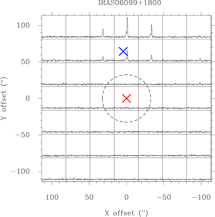
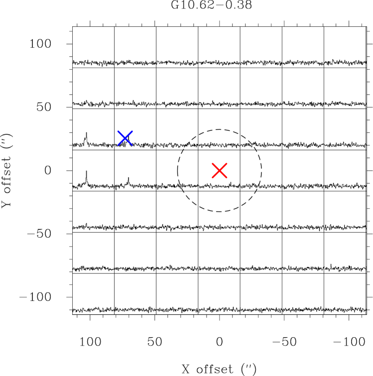
Figure 14: Map grids of 44 GHz CH₃OH masers of IRAS06099$+$1800 and G10.62$-$0.38. The red crosses indicate observed positions at the 1st and 2nd epochs in 2010 and 2011. On the other hand, the blue ones are positions of radio continuum sources taken from the catalogs of WC89a and KCW94 and they were used at the 3rd and 4th epochs in 2017. The dashed-circles correspond to a FWHM beam size (65″) at 44 GHz.

References

- Anglada (1995) Anglada, G. 1995, in Revista Mexicana de Astronomia y Astrofisica, vol. 27, Vol. 1, Revista Mexicana de Astronomia y Astrofisica Conference Series, ed. S. Lizano & J. M. Torrelles, 67
- Anglada et al. (1996) Anglada, G., Estalella, R., Pastor, J., Rodriguez, L. F., & Haschick, A. D. 1996, ApJ, 463, 205
- Araya et al. (2008) Araya, E., Hofner, P., Kurtz, S., Olmi, L., & Linz, H. 2008, ApJ, 675, 420
- Bachiller et al. (1990) Bachiller, R., Gomez-Gonzalez, J., Barcia, A., & Menten, K. M. 1990, A&A, 240, 116
- Bae et al. (2011) Bae, J.-H., Kim, K.-T., Youn, S.-Y., et al. 2011, ApJS, 196, 21
- Bartkiewicz et al. (2011) Bartkiewicz, A., Szymczak, M., Pihlström, Y. M., et al. 2011, A&A, 525, A120
- Bartkiewicz et al. (2009) Bartkiewicz, A., Szymczak, M., van Langevelde, H. J., Richards, A. M. S., & Pihlström, Y. M. 2009, A&A, 502, 155
- Beuther et al. (2003) Beuther, H., Schilke, P., & Stanke, T. 2003, A&A, 408, 601
- Beuther et al. (2002) Beuther, H., Walsh, A., Schilke, P., et al. 2002, A&A, 390, 289
- Breen et al. (2010a) Breen, S. L., Caswell, J. L., Ellingsen, S. P., & Phillips, C. J. 2010a, MNRAS, 406, 1487
- Breen et al. (2010b) Breen, S. L., Ellingsen, S. P., Caswell, J. L., & Lewis, B. E. 2010b, MNRAS, 401, 2219
- Breen et al. (2013) Breen, S. L., Ellingsen, S. P., Contreras, Y., et al. 2013, MNRAS, 435, 524
- Breen et al. (2015) Breen, S. L., Fuller, G. A., Caswell, J. L., et al. 2015, MNRAS, 450, 4109
- Bronfman et al. (1996) Bronfman, L., Nyman, L.-A., & May, J. 1996, A&AS, 115, 81
- Burns et al. (2015) Burns, R. A., Imai, H., Handa, T., et al. 2015, MNRAS, 453, 3163
- Carpenter et al. (1990) Carpenter, J. M., Snell, R. L., & Schloerb, F. P. 1990, ApJ, 362, 147
- Carral et al. (1999) Carral, P., Kurtz, S., Rodríguez, L. F., et al. 1999, Rev. Mexicana Astron. Astrofis., 35, 97
- Caswell et al. (1995) Caswell, J. L., Vaile, R. A., Ellingsen, S. P., Whiteoak, J. B., & Norris, R. P. 1995, MNRAS, 272, 96
- Caswell et al. (2010) Caswell, J. L., Fuller, G. A., Green, J. A., et al. 2010, MNRAS, 404, 1029
- Chambers et al. (2009) Chambers, E. T., Jackson, J. M., Rathborne, J. M., & Simon, R. 2009, ApJS, 181, 360
- Cheung et al. (1969) Cheung, A. C., Rank, D. M., & Townes, C. H. 1969, Nature, 221, 917
- Churchwell et al. (1990) Churchwell, E., Walmsley, C. M., & Cesaroni, R. 1990, A&AS, 83, 119
- Claussen et al. (1996) Claussen, M. J., Wilking, B. A., Benson, P. J., et al. 1996, ApJS, 106, 111
- Codella et al. (1996) Codella, C., Felli, M., & Natale, V. 1996, A&A, 311, 971
- Connelley et al. (2008) Connelley, M. S., Reipurth, B., & Tokunaga, A. T. 2008, AJ, 135, 2496
- Cragg et al. (1992) Cragg, D. M., Johns, K. P., Godfrey, P. D., & Brown, R. D. 1992, MNRAS, 259, 203
- Cragg et al. (2005) Cragg, D. M., Sobolev, A. M., & Godfrey, P. D. 2005, MNRAS, 360, 533
- de Villiers et al. (2014) de Villiers, H. M., Chrysostomou, A., Thompson, M. A., et al. 2014, MNRAS, 444, 566
- Durjasz et al. (2019) Durjasz, M., Szymczak, M., & Olech, M. 2019, MNRAS, 485, 777
- Elitzur et al. (1989) Elitzur, M., Hollenbach, D. J., & McKee, C. F. 1989, ApJ, 346, 983
- Ellingsen (2006) Ellingsen, S. P. 2006, ApJ, 638, 241
- Ellingsen et al. (2007) Ellingsen, S. P., Voronkov, M. A., Cragg, D. M., et al. 2007, in IAU Symposium, Vol. 242, Astrophysical Masers and their Environments, ed. J. M. Chapman & W. A. Baan, 213–217
- Felli et al. (1992) Felli, M., Palagi, F., & Tofani, G. 1992, A&A, 255, 293
- Felli et al. (2007) Felli, M., Brand, J., Cesaroni, R., et al. 2007, A&A, 476, 373
- Fontani et al. (2010) Fontani, F., Cesaroni, R., & Furuya, R. S. 2010, A&A, 517, A56
- Forster & Caswell (1989) Forster, J. R., & Caswell, J. L. 1989, A&A, 213, 339
- Furuya et al. (2003) Furuya, R. S., Kitamura, Y., Wootten, A., Claussen, M. J., & Kawabe, R. 2003, ApJS, 144, 71
- Furuya et al. (2001) Furuya, R. S., Kitamura, Y., Wootten, H. A., Claussen, M. J., & Kawabe, R. 2001, ApJ, 559, L143
- Gan et al. (2013) Gan, C.-G., Chen, X., Shen, Z.-Q., Xu, Y., & Ju, B.-G. 2013, ApJ, 763, 2
- Garay & Lizano (1999) Garay, G., & Lizano, S. 1999, PASP, 111, 1049
- Garay et al. (2002) Garay, G., Mardones, D., Rodríguez, L. F., Caselli, P., & Bourke, T. L. 2002, ApJ, 567, 980
- Genzel & Downes (1977) Genzel, R., & Downes, D. 1977, A&AS, 30, 145
- Goddi et al. (2015) Goddi, C., Henkel, C., Zhang, Q., Zapata, L., & Wilson, T. L. 2015, A&A, 573, A109
- Goddi & Moscadelli (2006) Goddi, C., & Moscadelli, L. 2006, A&A, 447, 577
- Goddi et al. (2011) Goddi, C., Moscadelli, L., & Sanna, A. 2011, A&A, 535, L8
- Goddi et al. (2007) Goddi, C., Moscadelli, L., Sanna, A., Cesaroni, R., & Minier, V. 2007, A&A, 461, 1027
- Goedhart et al. (2004) Goedhart, S., Gaylard, M. J., & van der Walt, D. J. 2004, MNRAS, 355, 553
- Gómez et al. (2010) Gómez, L., Luis, L., Hernández-Curiel, I., et al. 2010, ApJS, 191, 207
- Gomez et al. (1995) Gomez, Y., Rodriguez, L. F., & Marti, J. 1995, ApJ, 453, 268
- Gómez-Ruiz et al. (2016) Gómez-Ruiz, A. I., Kurtz, S. E., Araya, E. D., Hofner, P., & Loinard, L. 2016, ApJS, 222, 18
- Green et al. (2009) Green, J. A., Caswell, J. L., Fuller, G. A., et al. 2009, MNRAS, 392, 783
- Green et al. (2010) —. 2010, MNRAS, 409, 913
- Green et al. (2012) —. 2012, MNRAS, 420, 3108
- Gwinn et al. (1992) Gwinn, C. R., Moran, J. M., & Reid, M. J. 1992, ApJ, 393, 149
- Han et al. (2008) Han, S.-T., Lee, J.-W., Kang, J., et al. 2008, International Journal of Infrared and Millimeter Waves, 29, 69
- Harju et al. (1998) Harju, J., Lehtinen, K., Booth, R. S., & Zinchenko, I. 1998, A&AS, 132, 211
- Haschick et al. (1990) Haschick, A. D., Menten, K. M., & Baan, W. A. 1990, ApJ, 354, 556
- Hatchell et al. (2001) Hatchell, J., Fuller, G. A., & Millar, T. J. 2001, A&A, 372, 281
- Herbst & Racine (1976) Herbst, W., & Racine, R. 1976, AJ, 81, 840
- Hofner & Churchwell (1996) Hofner, P., & Churchwell, E. 1996, A&AS, 120, 283
- Hou & Han (2014) Hou, L. G., & Han, J. L. 2014, A&A, 569, A125
- Hu et al. (2016) Hu, B., Menten, K. M., Wu, Y., et al. 2016, ApJ, 833, 18
- Kalenskii et al. (2010) Kalenskii, S. V., Johansson, L. E. B., Bergman, P., et al. 2010, MNRAS, 405, 613
- Kalenskii et al. (2013) Kalenskii, S. V., Kurtz, S., & Bergman, P. 2013, Astronomy Reports, 57, 120
- Kang et al. (2015) Kang, H., Kim, K.-T., Byun, D.-Y., Lee, S., & Park, Y.-S. 2015, ApJS, 221, 6
- Kaufman & Neufeld (1996) Kaufman, M. J., & Neufeld, D. A. 1996, ApJ, 456, 250
- Kim et al. (2018a) Kim, C.-H., Kim, K.-T., & Park, Y.-S. 2018a, ApJS, 236, 31
- Kim & Kurtz (2006) Kim, K.-T., & Kurtz, S. E. 2006, ApJ, 643, 978
- Kim et al. (2011) Kim, K.-T., Byun, D.-Y., Je, D.-H., et al. 2011, Journal of Korean Astronomical Society, 44, 81
- Kim et al. (2018b) Kim, W. J., Urquhart, J. S., Wyrowski, F., Menten, K. M., & Csengeri, T. 2018b, A&A, 616, A107
- Kurtz et al. (1994) Kurtz, S., Churchwell, E., & Wood, D. O. S. 1994, ApJS, 91, 659
- Kurtz & Hofner (2005) Kurtz, S., & Hofner, P. 2005, AJ, 130, 711
- Kurtz et al. (2004) Kurtz, S., Hofner, P., & Álvarez, C. V. 2004, ApJS, 155, 149
- Lee et al. (2011) Lee, S.-S., Byun, D.-Y., Oh, C. S., et al. 2011, PASP, 123, 1398
- Lekht et al. (2006) Lekht, E. E., Trinidad, M. A., Mendoza-Torres, J. E., Rudnitskij, G. M., & Tolmachev, A. M. 2006, A&A, 456, 145
- Longmore et al. (2011) Longmore, S. N., Pillai, T., Keto, E., Zhang, Q., & Qiu, K. 2011, ApJ, 726, 97
- Martí et al. (1999) Martí, J., Rodríguez, L. F., & Torrelles, J. M. 1999, A&A, 345, L5
- Meehan et al. (1998) Meehan, L. S. G., Wilking, B. A., Claussen, M. J., Mundy, L. G., & Wootten, A. 1998, AJ, 115, 1599
- Mehringer & Menten (1997) Mehringer, D. M., & Menten, K. M. 1997, ApJ, 474, 346
- Menten (1991) Menten, K. 1991, in Astronomical Society of the Pacific Conference Series, Vol. 16, Atoms, Ions and Molecules: New Results in Spectral Line Astrophysics, ed. A. D. Haschick & P. T. P. Ho, 119
- Menten (1996) Menten, K. M. 1996, in IAU Symposium, Vol. 178, Molecules in Astrophysics: Probes & Processes, ed. E. F. van Dishoeck, 163–172
- Müller et al. (2004) Müller, H. S. P., Menten, K. M., & Mäder, H. 2004, A&A, 428, 1019
- Olech et al. (2019) Olech, M., Szymczak, M., Wolak, P., Sarniak, R., & Bartkiewicz, A. 2019, MNRAS, 486, 1236
- Palagi et al. (1993) Palagi, F., Cesaroni, R., Comoretto, G., Felli, M., & Natale, V. 1993, A&AS, 101, 153
- Palla et al. (1991) Palla, F., Brand, J., Comoretto, G., Felli, M., & Cesaroni, R. 1991, A&A, 246, 249
- Palla et al. (1993) Palla, F., Cesaroni, R., Brand, J., et al. 1993, A&A, 280, 599
- Pandian et al. (2007) Pandian, J. D., Goldsmith, P. F., & Deshpand e, A. A. 2007, ApJ, 656, 255
- Pety (2005) Pety, J. 2005, in SF2A-2005: Semaine de l’Astrophysique Francaise, ed. F. Casoli, T. Contini, J. M. Hameury, & L. Pagani, 721
- Plambeck & Menten (1990) Plambeck, R. L., & Menten, K. M. 1990, ApJ, 364, 555
- Pratap et al. (2008) Pratap, P., Shute, P. A., Keane, T. C., Battersby, C., & Sterling, S. 2008, AJ, 135, 1718
- Purcell et al. (2006) Purcell, C. R., Balasubramanyam, R., Burton, M. G., et al. 2006, MNRAS, 367, 553
- Rodriguez (1989) Rodriguez, L. F. 1989, Rev. Mexicana Astron. Astrofis., 18, 45
- Schuller et al. (2009) Schuller, F., Menten, K. M., Contreras, Y., et al. 2009, A&A, 504, 415
- Shepherd & Churchwell (1996) Shepherd, D. S., & Churchwell, E. 1996, ApJ, 457, 267
- Simon et al. (1981) Simon, M., Righini-Cohen, G., Felli, M., & Fischer, J. 1981, ApJ, 245, 552
- Slysh et al. (1994) Slysh, V. I., Kalenskii, S. V., Valtts, I. E., & Otrupcek, R. 1994, MNRAS, 268, 464
- Snell & Bally (1986) Snell, R. L., & Bally, J. 1986, ApJ, 303, 683
- Sobolev et al. (2007) Sobolev, A. M., Cragg, D. M., Ellingsen, S. P., et al. 2007, in IAU Symposium, Vol. 242, Astrophysical Masers and their Environments, ed. J. M. Chapman & W. A. Baan, 81–88
- Sridharan et al. (2002) Sridharan, T. K., Beuther, H., Schilke, P., Menten, K. M., & Wyrowski, F. 2002, ApJ, 566, 931
- Sugiyama et al. (2018) Sugiyama, K., Yonekura, Y., Motogi, K., et al. 2018, in IAU Symposium, Vol. 336, Astrophysical Masers: Unlocking the Mysteries of the Universe, ed. A. Tarchi, M. J. Reid, & P. Castangia, 45–48
- Szymczak et al. (2005) Szymczak, M., Pillai, T., & Menten, K. M. 2005, A&A, 434, 613
- Szymczak et al. (2012) Szymczak, M., Wolak, P., Bartkiewicz, A., & Borkowski, K. M. 2012, Astronomische Nachrichten, 333, 634
- Thompson et al. (2006) Thompson, M. A., Hatchell, J., Walsh, A. J., MacDonald, G. H., & Millar, T. J. 2006, A&A, 453, 1003
- Torrelles et al. (1997) Torrelles, J. M., Gómez, J. F., Rodríguez, L. F., et al. 1997, ApJ, 489, 744
- Torrelles et al. (2011) Torrelles, J. M., Patel, N. A., Curiel, S., et al. 2011, MNRAS, 410, 627
- Urquhart et al. (2009) Urquhart, J. S., Hoare, M. G., Lumsden, S. L., et al. 2009, A&A, 507, 795
- Urquhart et al. (2011) Urquhart, J. S., Morgan, L. K., Figura, C. C., et al. 2011, MNRAS, 418, 1689
- Urquhart et al. (2014) Urquhart, J. S., Moore, T. J. T., Csengeri, T., et al. 2014, MNRAS, 443, 1555
- Urquhart et al. (2015) Urquhart, J. S., Moore, T. J. T., Menten, K. M., et al. 2015, MNRAS, 446, 3461
- Valdettaro et al. (2001) Valdettaro, R., Palla, F., Brand, J., et al. 2001, A&A, 368, 845
- Voronkov et al. (2014) Voronkov, M. A., Caswell, J. L., Ellingsen, S. P., Green, J. A., & Breen, S. L. 2014, MNRAS, 439, 2584
- Voronkov et al. (2010) Voronkov, M. A., Caswell, J. L., Ellingsen, S. P., & Sobolev, A. M. 2010, MNRAS, 405, 2471
- Walsh et al. (1998) Walsh, A. J., Burton, M. G., Hyland, A. R., & Robinson, G. 1998, MNRAS, 301, 640
- Wang et al. (2006) Wang, Y., Zhang, Q., Rathborne, J. M., Jackson, J., & Wu, Y. 2006, ApJ, 651, L125
- Watson et al. (2003) Watson, C., Araya, E., Sewilo, M., et al. 2003, ApJ, 587, 714
- Wilking et al. (1994) Wilking, B. A., Claussen, M. J., Benson, P. J., et al. 1994, ApJ, 431, L119
- Wood & Churchwell (1989a) Wood, D. O. S., & Churchwell, E. 1989a, ApJS, 69, 831
- Wood & Churchwell (1989b) —. 1989b, ApJ, 340, 265
- Wouterloot et al. (1993) Wouterloot, J. G. A., Brand, J., & Fiegle, K. 1993, A&AS, 98, 589
- Wouterloot & Walmsley (1986) Wouterloot, J. G. A., & Walmsley, C. M. 1986, A&A, 168, 237
- Xu et al. (2003) Xu, Y., Zheng, X.-W., & Jiang, D.-R. 2003, Chinese J. Astron. Astrophys., 3, 49
- Zapata et al. (2009) Zapata, L. A., Ho, P. T. P., Schilke, P., et al. 2009, ApJ, 698, 1422
- Zhang et al. (2005) Zhang, Q., Hunter, T. R., Brand, J., et al. 2005, ApJ, 625, 864