Scalable Semi-Supervised SVM via Triply Stochastic Gradients

Abstract

Semi-supervised learning (SSL) plays an increasingly important role in the big data era because a large number of unlabeled samples can be used effectively to improve the performance of the classifier. Semi-supervised support vector machine (S³VM) is one of the most appealing methods for SSL, but scaling up S³VM for kernel learning is still an open problem. Recently, a doubly stochastic gradient (DSG) algorithm has been proposed to achieve efficient and scalable training for kernel methods. However, the algorithm and theoretical analysis of DSG are developed based on the convexity assumption which makes them incompetent for non-convex problems such as S³VM. To address this problem, in this paper, we propose a triply stochastic gradient algorithm for S³VM, called TSGS³VM. Specifically, to handle two types of data instances involved in S³VM, TSGS³VM samples a labeled instance and an unlabeled instance as well with the random features in each iteration to compute a triply stochastic gradient. We use the approximated gradient to update the solution. More importantly, we establish new theoretic analysis for TSGS³VM which guarantees that TSGS³VM can converge to a stationary point. Extensive experimental results on a variety of datasets demonstrate that TSGS³VM is much more efficient and scalable than existing S³VM algorithms.

1 Introduction

Algorithm	Reference	Method	Computational Complexity	Space Complexity
S3VMlight	Joachims (1999)	Self-labeling heuristics	$O(tn^{\kappa})$	$O(n^{2})$
NTS3VM	Chapelle (2007)	Gradient-based	$O(n^{3})$	$O(n^{2})$
BGS3VM	Le et al. (2016)	Gradient-based	$O(n^{3})$	$O(n^{2})$
BLS3VM	Collobert et al. (2006)	CCCP-based	$O(tn^{\kappa})$	$O(n^{2})$
ILS3VM	Gu et al. (2018d)	CCCP-based	$\approx O(Tn^{2})$	$O(n^{2})$
TSGS3VM	Our	TSG	$O(mT^{2})$	$O(T)$

Table 1: Comparisons of computational complexities and memory requirements of representative S³VM algorithms. ($n$ is the training size, $T$ is the total number of iteration, $t$ denotes the number of outer loops and $1<\kappa<2.3$)

Semi-supervised learning (SSL) plays an increasingly important role in the big data era because a large number of unlabeled samples can be used effectively to improve the performance of the classifier. Semi-supervised support vector machine (S³VM) Bennett and Demiriz (1999) is one of the most appealing methods for SSL. Specifically, S³VM enforces the classification boundary to go across the less-dense regions in the reproducing kernel Hilbert space (RKHS), while keeping the labeled data correctly classified. Unfortunately, this will lead to a non-convex optimization problem. It is well known that solving a non-convex optimization problem is normally difficult than solving a convex one like standard support vector machine. Under this arduous challenge, a wide spectrum of methods for S³VM have been proposed in the last two decades. Generally speaking, these methods can be roughly divided into three groups, i.e., methods with self-labeling heuristics, concave-convex procedure (CCCP) methods and gradient-based methods. We give a brief review of these representative S³VM methods in Section 2 and Table 1.

Unfortunately, these traditional S³VM methods are inefficient due to increased complexity introduced by the cost of kernel computation as well as non-convexity. Specifically, the kernel matrix needs $O(n^{2}d)$ operations to be calculated and $O(n^{2})$ memory to be stored, where $n$ denotes the size of training samples and $d$ denotes dimension of the data Gu et al. (2018b). Essentially, gradient-based S³VM methods have $O(n^{3})$ complexity due mainly to the operations on the kernel matrix. Even though a convex kernel problem can be solved by a state-of-the-art solver (e.g. LIBSVM), $O(n^{\kappa})$ computation is still needed where $1<\kappa<2.3$ Chang and Lin (2011). While to handle the non-convexity of S³VM, the methods using self-labeling heuristics and CCCP-based algorithms need to solve multiple convex sub-problems to guarantee that they finally converge Yuille and Rangarajan (2002). As a result, these methods scale as $O(tn^{\kappa})$, where $t$ denotes the number of solving sub-problems. We summarize the computational complexities and memory requirements of the representative S³VM methods in Table 1. As pointed in Gu et al. (2018d), scaling up S³VM is still an open problem.

Recently, a novel doubly stochastic gradient (DSG) method Dai et al. (2014) was proposed to achieve efficient and scalable training for kernel methods. Specifically, in each iteration, DSG computes a doubly stochastic gradient by sampling a random data sample and the corresponding random features to update the solution. Thus, DSG avoids computing and storing a kernel matrix, while enjoying nice computational and space complexities. Xie et al. Xie et al. (2015) used DSG to scale up nonlinear component analysis. To the best of our knowledge, Xie et al. (2015) is the only work based on DSG to solve a non-convex problem.

However, existing algorithms and theoretical analysis of DSG cannot be applied to S³VM due to the following two reasons. 1) Multiple data distributions: S³VM minimizes the training errors coming from two different sources. One is the expected error on the unlabeled data, and the other one is the mean error on the labeled data whose size is normally significantly smaller than the one of unlabeled data. However, DSG only considers the expected error on the labeled data. 2) Non-convexity analysis: The theoretical analysis in Xie et al. (2015) is based on a strong assumption (i.e., the initialization needs to be close to the optimum). However, such an assumption is rarely satisfied in practice. Besides, they focus on the nonlinear component analysis instead of general non-convex problems. Thus, it is infeasible to extend the analysis of Xie et al. (2015) to S³VM.

To address this challenging problem, we first propose a new and practical formulation of S³VM. Then, we develop a new triply stochastic gradient algorithm (TSGS³VM) to solve the corresponding optimization problem. Specifically, to handle two types of data instances involved in S³VM, TSGS³VM samples a labeled instance and an unlabeled instance as well with their random features in each iteration to compute a triply stochastic gradient (TSG). We then use the TSGs to iteratively update the solution. A critical question is whether and how fast this optimization process with multiple randomness would converge. In addressing this concern, we establish new theoretic analysis for TSGS³VM which guarantees that TSGS³VM can converge to a stationary point with a sublinear convergence rate for a general non-convex learning problem under weak assumptions. Extensive experimental results demonstrate the superiority of TSGS³VM.

Novelties. We summary the main novelties of this paper as follows.

1. To scale up S³VM, we propose a practical formulation of S³VM and develop a novel extension of DSG that could solve optimization problems with multiple data sources.

2. We have established the new theoretic analysis of TSGS³VM algorithm for a general non-convex learning problem which guarantees its convergence to a stationary point. To the best of our knowledge, it is the first work offering non-convex analysis for DSG-like algorithms without initialization assumption.

2 Related Works

We give a brief review of kernel approximation methods as well as the representative S³VM methods.

Kernel Approximation.

There are many kernel approximation methods proposed to address the scalability issue of kernel methods. For instance, low-rank factors are used to approximate the kernel matrix in Drineas and Mahoney (2005). Rahimi & Recht Rahimi and Recht (2008) provided another method that uses random features to approximate the map function explicitly. However, as analyzed in Drineas and Mahoney (2005); Lopez-Paz et al. (2014), the rank for low-rank and the number of random features need to be $O(n)$ to obtain a good generalization ability. To further improve the random features method, Dai et al. Dai et al. (2014) proposed DSG descent algorithm. Carratino et al. Carratino et al. (2018) proved that DSG only need $O(\sqrt{n})$ random features to obtain a good result. However, existing DSG methods Li et al. (2017); Gu et al. (2018c); Shi et al. (2019) can not be used for S³VM as discussed previously.

S³VM Methods.

As mentioned above, traditional S³VM methods can be roughly divided into three types, i.e., the method of self-labeling heuristics, the concave-convex procedure (CCCP) method, and the gradient-based method. For the method of self-labeling heuristics, Joachims Joachims (1999) proposed a S³VM^light algorithm which uses self-labeling heuristics for labeling the unlabeled data, then iteratively solve this standard SVM until convergence. CCCP-based methods were proposed to solve S³VM in Chapelle and Zien (2005); Wang et al. (2007); Yu et al. (2019). The basic principle of CCCP is to linearize the concave part of S³VM’s objective function around a solution obtained in the current iteration so that sub-problem is convex. Then the CCCP framework solves a sequence of the convex sub-problem iteratively until decision variable converges. Based on CCCP framework, Gu et al. Gu et al. (2018d) proposed an incremental learning method for S³VM which is suitable for the online scenario. For gradient-based methods, Chapelle and Zien Chapelle and Zien (2005) approximate the kernel matrix $K$ using low-rank factors, then using gradient descent to solve S³VM on the low-rank matrix. BGS³VM Le et al. (2016) uses budgeted SGD to limit the model size to two predefined budgets $B_{l}$ and $B_{u}$.

3 Preliminaries

In this section, we first give a general non-convex learning problem for S³VM, and then give a brief review of random feature approximation.

Name	$u(r)$	$u^{\prime}(r)$
SHG	$\max\{0,1-|r|\}$	$\left\{\begin{matrix}0&{\rm if}\ |r|\geq 1\\ -1&{\rm if}\ |r|<1\end{matrix}\right.$
SSHG	$\frac{1}{2}\max\{0,1-|r|\}^{2}$	$\left\{\begin{matrix}0&{\rm if}\ |r|\geq 1\\ |r|-1&{\rm if}\ |r|<1\end{matrix}\right.$
Ramp	$H_{1}(r)-H_{s}(r)$	$H^{\prime}_{1}(r)-H^{\prime}_{s}(r)$
DA	$\exp(-5r^{2})$	$-10r\cdot\exp(-5r^{2})$

Table 2: Summary of the non-convex loss functions used in S³VM, where $H_{s}(\cdot)=\max\{0,s-\cdot\}$, then $H^{\prime}_{s}(\cdot)=0$, if $\cdot\geq s$ else $H^{\prime}_{s}(\cdot)=-1$. SHG, SSHG and DA denote symmetric hinge, square SHG and a differentiable approximation to SSHG respectively.

3.1 S³VM Optimization Formulation

Given the training dataset $\cal X$ constituted with $n^{l}$ labeled examples $\mathcal{L}:=\{({x}_{i},y_{i})\}_{i=1}^{n^{l}}$ and $n^{u}$ unlabeled examples $\mathcal{U}:=\{{x}_{i}\}_{i=n^{l}+1}^{n}$, where $n=n^{l}+n^{u}$, ${x_{i}}\in\mathbb{R}^{d}$, and $y_{i}\in\{1,-1\}$. Traditional S³VM solves the following problem.

$$\min_{f\in\cal H}\quad \frac{1}{2}||f||^{2}_{\cal H}+\frac{C}{n^{l}}\sum_{(x,y)\in\mathcal{L}}l(f(x),y)+\frac{C^{*}}{n^{u}}\sum_{x\in\mathcal{U}}u(f(x))$$

where $C$ and $C^{*}$ are regularization parameters, $||\cdot||_{\cal H}$ denotes the norm in RKHS, $l(r,v)=\max(0,1-vr)$ is the hinge loss, its subgradient $l^{\prime}(r,v)=0$, if $rv\geq 1$, else $l^{\prime}(r,v)=-v$, $u(r)$ is the non-convex loss function which enforce unlabeled data away from the discrimination hyperplane. We summarize the commonly used non-convex S³VM losses and its subgradient $u^{\prime}(r)$ in Table 2.

For S³VM problems, however, the volumes of labeled and unlabeled data are usually quite different. Because of the labeling cost, the labeled dataset is often very small, while a large amount of unlabeled data can be obtained relatively easily. Taking this into consideration, we propose to solve a novel S³VM formulation as follows.

$$\min_{f\in\cal H}R(f)$$

$$= \frac{1}{2}||f||^{2}_{\cal H}+\frac{C}{n^{l}}\sum_{(x,y)\in\mathcal{L}}l(f(x),y)+C^{*}\mathbb{E}_{x\sim P(x)}u(f(x))$$

where $P(x)$ denotes the target data distribution. Notice that we use the empirical mean error on the labeled dataset, while using the expected error on the whole distribution for the unlabeled data.

3.2 Random Feature Approximation

Random feature is a powerful technique to make kernel methods scalable. It uses the intriguing duality between kernels and stochastic processes. Specifically, according to the Bochner theorem Wendland (2004), for any positive definite PD kernel $k(\cdot,\cdot)$, there exists a set $\Omega$, a probability measure $\mathbb{P}$ and a random feature map $\phi_{\omega}(x)$, such that $k(x,x^{\prime})=\int_{\Omega}\phi_{\omega}(x)\phi_{\omega}(x^{\prime})d\mathbb{P}(\omega)$. In this way, the value of the kernel function can be approximated by explicitly computing random features $\phi_{\omega}(x)=[\frac{1}{\sqrt{m}}\phi_{\omega_{1}}(x),\frac{1}{\sqrt{m}}\phi_{\omega_{2}}(x),\cdots,\frac{1}{\sqrt{m}}\phi_{\omega_{m}}(x)]$, i.e.,

$$k(x,x^{\prime})\approx\frac{1}{m}\sum_{i=1}^{m}\phi_{\omega_{i}}(x)\phi_{\omega_{i}}(x^{\prime})$$ (2)

where $m$ is the number of random features. Using Gaussian RBF kernel as a concrete example, it yields a Gaussian distribution $\mathbb{P}(\omega)$ over random feature maps of Fourier basis functions $\phi_{\omega_{i}}(x)=\sqrt{2}cos({\omega_{i}^{T}x+b})$ to compute its feature mapping, where $\omega_{i}$ is drawn from $\mathbb{P}(\omega)$ and $b$ is drawn uniformly form $[0,2\pi]$. Moreover, many random feature construction methods have been proposed for various kernels, such as dot-product kernels and Laplacian kernels.

The theory of RKHS provides a rigorous mathematical framework for studying optimization problems in the functional space. Specifically, we know that every PD kernel $k(x,x^{\prime})$ has a corresponding RKHS $\mathcal{H}$. An RKHS $\mathcal{H}$ has the reproducing property, i.e., $\forall x\in\mathcal{X},\forall f\in\mathcal{H}$, we always have $\langle f(\cdot),k(x,\cdot)\rangle_{\mathcal{H}}=f(x)$. Besides, functional gradient in RKHS $\mathcal{H}$ can be computed as $\nabla f(x)=k(x,\cdot)$ and $\nabla||f||^{2}_{\mathcal{H}}=2f$.

4 Triply Stochastic S³VM

The above section has introduced the basic theoretic tools for triply stochastic functional gradient descent. Now we introduce how to utilize these tools to solve the S³VM problem.

4.1 Triply Stochastic Gradient

From Eq. (3.1), it is not hard to notice that $R(f)$ involves two different data sources. Taking into consideration the distribution of random features $\omega\sim\mathbb{P}(\omega)$ would give us three sources of possible randomness. Here we will show how to explicitly compute the stochastic gradient with these three sources of randomness.

Stochastic Functional Gradients.

Naturally, to iteratively update $f$ in a stochastic manner, we need to sample instances from the labeled dataset as well as the whole distribution. Different from DSG, we here randomly sample a pair of data points, from the labeled and the unlabeled data distributions, respectively. Then we can obtain stochastic functional gradients for $R(f)$ with these two data points as follow,

$$g(\cdot)=f(\cdot)+\xi(\cdot)$$ (3)

where $\xi(\cdot)$ is the gradient contributed by the loss from both labeled and unlabeled data. It can be computed using the chain rule

$$\xi(\cdot)=Cl^{\prime}(f(x^{l}),y^{l})k(x^{l},\cdot)+C^{*}u^{\prime}(f(x^{u}))k(x^{u},\cdot)$$ (4)

where $x^{l}$, $x^{u}$ are sampled from the labeled dataset and unlabeled distribution $P(x)$ respectively. Next we will plugging the random feature approximation technique described in the previous section.

Random Feature Approximation.

According to Eq. (2), when we use stochastically generated random feature $\omega$, we can further approximate $\xi(\cdot)$ as:

$$\xi(\cdot)\approx\zeta(\cdot)$$ (5)

$$= Cl^{\prime}(f(x^{l}),y^{l})\phi_{\omega}(x^{l})\phi_{\omega}(\cdot)+C^{*}u^{\prime}(f(x^{u}))\phi_{\omega}(x^{u})\phi_{\omega}(\cdot)$$

note that $\xi(\cdot)=\mathbb{E}_{\omega}[\zeta(\cdot)]$. This leads to an unbiased estimator of the original functional gradient with three layers of stochasticity, i.e.,

$$\nabla R(f)=\mathbb{E}_{(x^{l},y^{l})\in\mathcal{L}}\mathbb{E}_{x^{u}\sim P(x)}\mathbb{E}_{\omega}(\zeta(\cdot))+f(\cdot)$$ (6)

Since three random events occur per iteration, i.e. $x^{l}$, $x^{u}$, $\omega$, we call our approximate functional gradient as triply stochastic functional gradient.

Update Rules.

In the $t$-th iteration, the triply stochastic (functional) gradient update rule for $f$ is:

$$f_{t+1}(\cdot)=f_{t}(\cdot)-\gamma_{t}(\zeta_{t}(\cdot)+f_{t}(\cdot))=\sum_{i=1}^{t}a^{i}_{t}\zeta_{i}(\cdot)$$ (7)

where $\gamma$ denotes the step size and the initial value $f_{1}(\cdot)=0$. It is straight forward to calculate that $a_{t}^{i}=-\gamma_{i}\prod_{k=i+1}^{t}(1-\gamma_{k})$. Ideally, if we could somehow compute the stochastic (functional) gradients $\xi_{j}(\cdot)$, the update rule becomes:

$$h_{t+1}(\cdot)=h_{t}(\cdot)-\gamma_{t}(\xi_{t}(\cdot)+h_{t}(\cdot))=\sum_{i=1}^{t}a^{i}_{t}\xi_{i}(\cdot)$$ (8)

where we have used $h_{t+1}$ instead of $f_{t+1}$ to distinguish from the triply stochastic (functional) gradient update rule and $h_{1}(\cdot)=0$. However, to avoid the expense of kernel computation, our algorithm will use the triply stochastic update rule Eq. (7) instead of Eq. (8).

4.2 Algorithm

Based on the above triply stochastic gradient update rules (7), we provide the TSGS³VM training and prediction procedures in Algorithms 1 and 2 receptively. Notice that directly computing all the random features still needs a large amount of memory. Following the pseudo-random number generators setting of Dai et al. (2014), our random feature generator is initialized by a predefined seed according to iteration. Thus, TSGS³VM does not need to save the random feature matrix which makes it more memory friendly. In the $i$-th iteration, our method will execute the following steps.

1. Sample data pair (lines 2-3 in Algorithm 1): Stochastically sample a labeled sample $(x^{l}_{i},y^{l}_{i})$ and an unlabeled sample $x^{u}_{i}$ from different distribution respectively.

2. Sample random features (line 4 in Algorithm 1): Stochastically sample $\omega^{i}\sim\mathbb{P}(\omega)$ with seed $i$ and generate random features.

3. Update coefficients (lines 5-8 in Algorithm 1): Evaluate function value and update $f$ according to Eq. (7).

Remark 1

For each iteration, TSGS³VM needs $O(mT)$ operations to evaluate function value, since evaluating the function value needs generating $m$ random features ($O(m)$) for $T$ times. Thus, the total computational complexity of TSGS³VM is $O(mT^{2})$. Due to the use of random features and pseudo-random method, TSGS³VM only requires $O(T)$ memory, where $T$ is the iteration number.

Algorithm 1 TSGS³VM Train

0:  ${\cal L},P(x),\mathbb{P}(\omega),\phi_{\omega}(x),u(f(x)),C,C^{*}$

1:  for $i=1,\cdots,T$ do

2:     Sample $(x_{i}^{l},y_{i}^{l})\sim\mathcal{L}$

3:     Sample $x_{i}^{u}\sim P(x)$

4:     Sample $\omega_{i}\sim\mathbb{P}(\omega)$ with seed $i$

5:     $f(x^{l}_{i})=\textbf{Predict}(x^{l}_{i},\{\alpha_{j}\}_{j=1}^{i-1})$

6:     $f(x^{u}_{i})=\textbf{Predict}(x^{u}_{i},\{\alpha_{j}\}_{j=1}^{i-1})$

7:     $\alpha_{i}=-\gamma_{i}(Cl^{\prime}(f(x^{l}_{i}),y^{l}_{i})\phi_{\omega_{i}}(x^{l}_{i})+C^{*}u^{\prime}(f(x^{u}_{i}))\phi_{\omega_{i}}(x^{u}_{i}))$

8:     $\alpha_{j}=(1-\gamma_{i})\alpha_{j}$, for $j=1,\cdots,i-1$

9:  end for

9:  $\{\alpha_{i}\}_{i=1}^{T}$.

Algorithm 2 TSGS³VM Predict

0:  $\mathbb{P}(\omega),\phi_{\omega}(x),x,\{\alpha_{i}\}_{i=1}^{T}$

1:  Set $f(x)=0$

2:  for $i=1,\cdots,T$ do

3:     Sample $\omega_{i}\sim\mathbb{P}(\omega)$ with seed $i$

4:     $f(x)=f(x)+\alpha_{i}\phi_{\omega_{i}}(x)$

5:  end for

5:  $f(x)$

5 Theoretical Guarantees

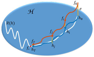
Figure 1: Illustration of how TSGS³VM converge to a stationary point, where $e$ denotes for the error between $f_{t}$ and $h_{t}$, the white line denote the objective value $R(h)$. In this toy model we assume all horizontal points in $\cal H$ have the same objective value.

We follow the common goal of non-convex analysis Ghadimi and Lan (2013); Gu et al. (2018a); Huo et al. (2018) to bound $\mathbb{E}||\nabla R(f)||^{2}$, which means that the objective function will converge (in expectation) to a stationary point $f_{*}$. When we use the hypothetical update rule (8), $h_{t}$ will always be inside of $\cal H$. However, because we could only use random features to approximate $h_{t}$ with $f_{t}$, we face the risk that functional $f_{t}$ could be outside of $\cal H$. As a consequence, $\mathbb{E}||\nabla R(f)||^{2}_{\cal H}=0$ is not the stationary point of the objective function (3.1). From Eq. (7) and Eq. (8), it is obvious that every update of $h_{t}$ happens implicitly with an update of $f_{t}(x)$. According to this relationship, we proposed to divide the analysis in two parts. As illustrated in Fig. 1, for a general non-convex optimization problem $R(h)$, we prove that the $h_{t+1}$ converges to a stationary point $f_{*}$ (i.e., $\mathbb{E}||\nabla R(h_{t+1})||^{2}_{\cal H}<\epsilon_{1}$) firstly. Then we prove that $f_{t+1}(x)$ keeps close to its hypothetic twin $h_{t+1}(x)$ for any $x\in\cal X$ (i.e., $|f_{t+1}(x)-h_{t+1}(x)|^{2}<\epsilon_{2}$).

Dataset	Dimensionality	Samples	Source
CodRNA	8	59,535	LIBSVM
W6a	300	49749	LIBSVM
IJCNN1	22	49,990	LIBSVM
SUSY	18	5,000,000	LIBSVM
Skin	3	245,057	LIBSVM
Higgs	28	1,100,000	LIBSVM
Dota2	16	102,944	UCI
HEPMASS	28	10,500,000	UCI

Table 3: Datasets used in the experiments.

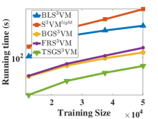
(a) CodRNA

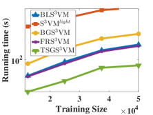
(b) W6a

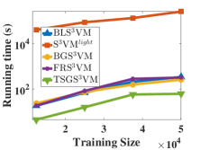
(c) IJCNN1

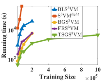
(d) SUSY

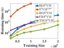
(e) Skin

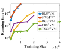
(f) Higgs

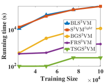
(g) Dota2

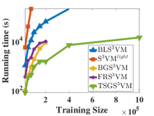
(h) HEPMASS

Figure 2: Running time of different S³VM solvers v.s. training size on the eight benchmark data sets, where the lines of BLS³VM and S³VM^light are incomplete on several datasets due to the corresponding implementations crash on the large-scale training set.

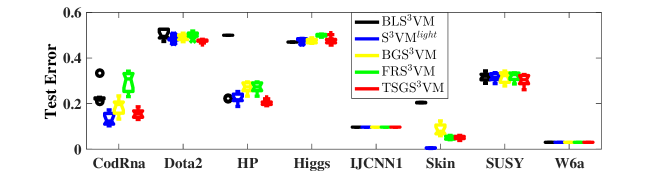
Figure 3: The boxplot of test error for different methods on different datasets.

Our analysis is built upon the following assumptions which are standard for the analysis of non-convex optimization and DSG Dai et al. (2014).

Assumption 1

(Lipschitzian gradient) The gradient function $\nabla R(f)$ is Lipschitzian, that is to say

$$||\nabla R(f)-\nabla R(g)||_{\cal H}\leq L||f-g||_{\cal H},\forall f,g\in\cal H$$ (9)

Assumption 2

(Lipschitz continuity) $l(r,v)$ is $L^{\prime}$-Lipschitz continuous in terms of its 1st argument. $u(r,v)$ is $U^{\prime}$-Lipschitz continuous in terms of its 1st argument. We further denote $M^{\prime}=CL^{\prime}+C^{*}U^{\prime}$.

Assumption 3

(Bound of derivative) The derivatives are bounded: $|l^{\prime}|<M^{l}$ and $|u^{\prime}|<M^{u}$, where $l^{\prime}$ and $u^{\prime}$ is the derivative of $l(r,v)$ and $u(r)$ w.r.t. the 1st argument respectively. We further denote $M=CM^{l}+C^{*}M^{u}$.

Assumption 4

(Bound of kernel and random features) We have an upper bound for the kernel value, $k(x,x^{\prime})\leq\kappa$. There is an upper bound of random feature norm, i.e., $|\phi_{\omega}(x)\phi_{\omega}(x^{\prime})|\leq\phi$.

Suppose the total number of iterations is $T$, we introduce our main theorems as below. All the detailed proofs are provided in our Appendix.

Theorem 1

For any $x\in\cal X$, fix $\gamma=\frac{\theta}{T^{3/4}}$ with $0<\theta\leq T^{3/4}$, we have

$$\mathbb{E}_{x^{l},x^{u},\omega_{t}}\Big{[}\Big{|}f_{t}(x)-h_{t}(x)\Big{|}^{2}\Big{]}\leq\dfrac{D}{T^{1/2}}$$ (10)

where $D=\theta^{2}M^{2}(\sqrt{\kappa}+\sqrt{\phi})^{2}$.

Remark 2

The error between $f_{t+1}$ and $h_{t+1}$ is mainly induced by random features. Theorem 1 shows that this error has the convergence rate of $O(1/\sqrt{T})$ with proper step size.

Theorem 2

For fixed $\gamma=\frac{\theta}{T^{3/4}}$, $0<\theta\leq T^{3/4}$, we have that

$$\mathbb{E}_{x^{l},x^{u},\omega_{t}}[||\nabla R(h_{t})||^{2}_{\cal H}]\leq\frac{E}{T^{1/4}}+\frac{F}{{T}^{3/4}}$$ (11)

where $E=\frac{1}{\theta}[R(h_{1})-R^{*}]+\theta M^{2}M^{\prime}(\sqrt{\kappa}+\sqrt{\phi})\kappa,F=2\theta M^{2}L\kappa$, $R^{*}$ denotes the optimal value of (3.1).

Remark 3

Instead of using the convexity assumption in Dai et al. (2014), Theorem 2 uses Lipschitzian gradient assumption to build the relationship between gradients and the updating functions $h_{t+1}$. Thus, we can bound each error term of $\mathbb{E}_{x^{l},x^{u},\omega_{t}}[||\nabla R(h_{t})||^{2}_{\cal H}]$ as shown in Appendix. Note that compared to the strong assumption (i.e., the good initialization) used in Xie et al. (2015), the assumptions used in our proofs are weaker and more realistic.

6 Experiments and Analysis

In this section, we will evaluate the practical performance of TSGS³VM when comparing against other state-of-the-art solvers.

6.1 Experimental Setup

To show the advantage our TSGS³VM for large-scale S³VM learning, we conduct the experiments on large scale datasets to compare TSGS³VM with other state-of-the-art algorithms in terms of predictive accuracy and time consumption. Specifically, the compared algorithms in our experiments are summarized as follows.

1. BLS³VM Collobert et al. (2006): The state-of-art S³VM algorithm based on CCCP and SMO algorithm Cai and Cherkassky (2012).

2. S³VM^light Joachims (1999): The implementation in the popular S³VM^light software. It is based on the local combinatorial search guided by a label switching procedure.

3. BGS³VMLe et al. (2016): Our implementation of BGS³VM in MATLAB.

4. FRS³VM: Standard SGD with fixed random features.

5. TSGS³VM: Our proposed S³VM algorithm via triply stochastic gradients.

Implementation.

We implemented the TSGS³VM algorithm in MATLAB. For the sake of efficiency, our TSGS³VM implementation also uses a mini-batch setting. We perform experiments on Intel Xeon E5-2696 machine with 48GB RAM. The Gaussian RBF kernel $k(x,x^{\prime})=\exp(-\sigma||x-x^{\prime}||^{2})$ and the loss function $u=\max\{0,1-|r|\}$ was used for all algorithms. 5-fold cross-validation was used to determine the optimal settings (test error) of the model parameters (the regularization factor C and the Gaussian kernel parameter $\sigma$), the parameters $C^{*}$ was set to $C\frac{n^{l}}{n^{u}}$. Specifically, the unlabeled dataset was divided evenly to 5 subsets, where one of the subsets and all the labeled data are used for training, while the other 4 subsets are used for testing. Parameter search was done on a 7$\times$7 coarse grid linearly spaced in the region $\{\log_{10}C,\log_{10}\sigma)|-3\leq\log_{10}C\leq 3,-3\leq\log_{10}\sigma\leq 3\}$ for all methods. For TSGS³VM, the step size $\gamma$ equals $\frac{1}{\eta}$, where $0\leq\log_{10}{\eta}\leq 3$ is searched after $C$ and $\sigma$. Besides, the number of random features is set to be $\lceil\sqrt{n}\rceil$ and the batch size is set to 256. The test error was obtained by using these optimal model parameters for all the methods. To achieve a comparable accuracy to our TSGS³VM, we set the minimum budget sizes $B_{l}$ and $B_{u}$ as $100$ and $0.2*n_{u}$ respectively for BG$S^{3}$VM. We stop TSGS³VM and BG$S^{3}$VM after one pass over the entire dataset. We stop FRS³VM after 10 pass over the entire dataset to achieve a comparable accuracy. All results are the average of 10 trials.

Datasets.

Table 3 summarizes the 8 datasets used in our experiments. They are from LIBSVM and UCI repositories. Since all these datasets are originally labeled, we intentionally randomly sample 200 labeled instances and treat the rest of data as unlabeled to make a semi-supervised learning setting.

6.2 Experimental Results

Fig. 2 shows the test error v.s. the training size for different algorithms. The results clearly show that TSGS³VM runs much faster than other methods. Specifically, Figs. 2d and 2h confirm the high efficiency of TSGS³VM even on the datasets with one million samples. Besides, TSGS³VM requires low memory benefiting from pseudo-randomness for generating random features, while BLS³VM and S³VM^light would be often out of memory on large scale datasets.

Fig. 3 shows the test error of different methods. The results were obtained at the optimal hyper-parameters for different algorithms. From the figure, it is clear that TSGS³VM achieves similar generalization performance as that of BLS³VM, S³VM^light, and BGS³VM methods which confirm that TSGS³VM converge well in practice. Besides, TSGS³VM achieves better generalization performance than FRS³VM, because TSGS³VM has the advantage that it would automatically use more and more random features (for each data $x$) as the number of iterations increases.

Based on these results, we conclude that TSGS³VM is much more efficient and scalable than these algorithms while retaining the similar generalization performance.

7 Conclusion

In this paper, we provide a novel triply stochastic gradients algorithm for kernel S³VM to make it scalable. We establish new theoretic analysis for TSGS³VM which guarantees that TSGS³VM can efficiently converge to a stationary point for a general non-convex learning problem under weak assumptions. As far as we know, TSGS³VM is the first work that offers non-convex analysis for DSG-like algorithm without a strong initialization assumption. Extensive experimental results on a variety of benchmark datasets demonstrate the superiority of our proposed TSGS³VM.

Appendix A Proof of Theorem 1

To proof theorem 1, we first give lemma 1 as follows

Lemma 1

For any $x\in\cal X$, consider a fix step size $\gamma$, and $0<\gamma\leq 1$, we have that

$$\mathbb{E}_{x^{l},x^{u},\omega_{t}}\Big{[}\Big{|}f_{t}(x)-h_{t}(x)\Big{|}^{2}\Big{]}\leq B^{2}_{1,t+1}$$ (12)

where $B^{2}_{1,t+1}:=M^{2}(\sqrt{\kappa}+\sqrt{\phi})^{2}t\gamma^{2}$, and $B_{1,1}=0$.

Proof. We denote $W_{i}(x)=W_{i}(x;x_{i}^{l},x_{i}^{u},\omega_{i})=a_{t}^{i}(\zeta^{i}(x)-\xi^{i}(x))$. Based on the definition and assumptions in main body, $W_{i}(x)$ is bounded as follows

$$\quad\quad|W_{i}(x)|$$

$$\leq\quad c_{i}=\quad|a_{t}^{i}|(|\zeta_{i}(x)|+|\xi_{i}(x)|)$$

$$=\quad|a_{t}^{i}|\big{[}|Cl^{\prime}(f(x_{i}^{l}),y_{i}^{l})k(x_{i}^{l},x)+C^{*}u^{\prime}(f(x_{i}^{u}))k(x_{i}^{u},x)|$$

$$\quad+|Cl^{\prime}(f(x_{i}^{l}),y_{i}^{l})\phi_{\omega_{i}}(x_{i}^{l})\phi_{\omega_{i}}(x)$$

$$\quad+C^{*}u^{\prime}(f(x_{i}^{u}))\phi_{\omega_{i}}(x_{i}^{l})\phi_{\omega_{i}}(x)|\big{]}$$

$$\leq\quad|a_{t}^{i}|\big{[}(CM^{l}+C^{*}M^{u})(\sqrt{\kappa}+\sqrt{\phi})\big{]}$$

$$=\quad M(\sqrt{\kappa}+\sqrt{\phi})|a_{t}^{i}|$$ (13)

Based on the definition of $a_{t}^{t}$, $|a_{t}^{t}|\leq\gamma$, and for any $i$ we have $|a_{t}^{i}|\leq\gamma\prod_{j=i+1}^{t}(1-\gamma)\leq\gamma$ due to $0<\gamma\leq 1$. Consequently, $\sum_{i=1}^{t}|a_{t}^{i}|^{2}\leq t\gamma^{2}$. Then we have $\mathbb{E}_{x^{l}_{t},x^{u}_{t},\omega_{t}}\Big{[}\Big{|}f_{t}(x)-h_{t}(x)\Big{|}^{2}\Big{]}\leq M^{2}(\sqrt{\kappa}+\sqrt{\phi})^{2}\sum_{i=1}^{t}|a_{t}^{i}|^{2}\leq M^{2}(\sqrt{\kappa}+\sqrt{\phi})^{2}t\gamma^{2}$. We obtain the Lemma 1. Taking $\gamma=\frac{\theta}{T^{3/4}}$, we have

$$B^{2}_{1,t+1} :=\quad M^{2}(\sqrt{\kappa}+\sqrt{\phi})^{2}t\frac{\theta^{2}}{T^{3/2}}$$

$$\leq\quad M^{2}(\sqrt{\kappa}+\sqrt{\phi})^{2}T\frac{\theta^{2}}{T^{3/2}}$$

$$\leq\quad M^{2}(\sqrt{\kappa}+\sqrt{\phi})^{2}\frac{\theta^{2}}{T^{1/2}}$$ (14)

then we obtain theorem 1.

Appendix B Proof of Theorem 2

Proof For the sake of simple notations, let us first denote the following three different gradient terms, which are

$$g_{t} =\quad\xi_{t}+h_{t}$$

$$=\quad Cl^{\prime}(f_{t}(x_{t}^{l}),y_{t}^{l})k(x_{t}^{l},\cdot)$$

$$\quad+C^{*}u^{\prime}(f_{t}(x_{t}^{u}))k(x_{t}^{u},\cdot)+h_{t}$$

$$\hat{g}_{t} =\quad\hat{\xi}_{t}+h_{t}$$

$$=\quad Cl^{\prime}(h_{t}(x_{t}^{l}),y_{t}^{l})k(x_{t}^{l},\cdot)$$

$$\quad+C^{*}u^{\prime}(h_{t}(x_{t}^{u}))k(x_{t}^{u},\cdot)+h_{t}$$

$$\nabla R(h_{t}) =\quad\mathbb{E}_{x^{l},x^{u}}[\hat{g}_{t}]$$

$$=\quad\mathbb{E}_{x^{l},x^{u}}[Cl^{\prime}(h_{t}(x_{t}^{l}),y_{t}^{l})k(x_{t}^{l},\cdot)$$

$$\quad+C^{*}u^{\prime}(h_{t}(x_{t}^{u}))k(x_{t}^{u},\cdot)]+h_{t}$$

Besides, we use $\mathbb{E}$ to denotes $\mathbb{E}_{x^{l}_{t},x^{u}_{t},\omega_{t}}$ for simplicity sometimes. Similar as Ghadimi and Lan (2013); Reddi et al. (2016), using the assumption 1 and $h_{t+1}=h_{t}-\gamma g_{t},\forall t\geq 1$, for $t=1,\cdots,T$ we have

$$\quad\quad R(h_{t+1})$$

$$\leq\quad R(h_{t})+\langle\nabla R(h_{t}),h_{t+1}-h_{t}\rangle+\frac{L}{2}||h_{t+1}-h_{t}||^{2}_{\cal H}$$

$$=\quad R(h_{t})-\gamma\langle\nabla R(h_{t}),g_{t}\rangle+\frac{L\gamma^{2}}{2}||g_{t}||^{2}_{\cal H}$$

$$=\quad R(h_{t})-\gamma\langle\nabla R(h_{t}),g_{t}-\hat{g}_{t}+\hat{g}_{t}-\nabla R(h_{t})$$

$$\quad+\nabla R(h_{t})\rangle+\frac{L\gamma^{2}}{2}||g_{t}||^{2}_{\cal H}$$

$$=\quad R(h_{t})-\gamma||\nabla R(h_{t})||^{2}_{\cal H}+\gamma\langle\nabla R(h_{t}),\hat{g}_{t}-g_{t}\rangle$$

$$\quad+\gamma\langle\nabla R(h_{t}),\nabla R(h_{t})-\hat{g}_{t}\rangle+\frac{L\gamma^{2}}{2}||g_{t}||^{2}_{\cal H}$$ (15)

Summing up the above inequalities from and re-arranging the terms, we obtain

$$\quad\quad\frac{1}{T}\sum_{t=1}^{T}\gamma||\nabla R(h_{t})||^{2}_{\cal H}$$

$$\leq\quad\frac{1}{T}\big{[}R(h_{1})-R(h_{T+1})+\sum_{t=1}^{T}\gamma\langle\nabla R(h_{t}),\hat{g}_{t}-g_{t}\rangle$$

$$\quad+\sum_{t=1}^{T}\gamma\langle\nabla R(h_{t}),\nabla R(h_{t})-\hat{g}_{t}\rangle+\sum_{t=1}^{T}\frac{L\gamma^{2}}{2}||g_{t}||^{2}_{\cal H}\big{]}$$

$$\leq\quad\frac{1}{T}\big{[}R(h_{1})-R^{*}+\sum_{t=1}^{T}\gamma\langle\nabla R(h_{t}),\hat{g}_{t}-g_{t}\rangle$$

$$\quad+\sum_{t=1}^{T}\gamma\langle\nabla R(h_{t}),\nabla R(h_{t})-\hat{g}_{t}\rangle+\sum_{t=1}^{T}\frac{L\gamma^{2}}{2}||g_{t}||^{2}_{\cal H}\big{]}$$ (16)

where $R^{*}$ is the optimal value of $R(h_{t})$ and the last inequality follows from the fact that $R(h_{T+1})\geq R^{*}$. Taking expectations on both sides we have

$$\quad\quad\mathbb{E}[||\nabla R(h_{t})||^{2}_{\cal H}]$$

$$\leq\quad\frac{1}{T\gamma}\big{[}R(h_{1})-R^{*}\big{]}+\mathbb{E}\big{[}\langle\nabla R(h_{t}),\hat{g}_{t}-g_{t}\rangle\big{]}$$

$$\quad+\mathbb{E}\big{[}\langle\nabla R(h_{t}),\nabla R(h_{t})-\hat{g}_{t}\rangle\big{]}+\frac{L\gamma}{2}\mathbb{E}\big{[}||g_{t}||^{2}_{\cal H}\big{]}$$ (17)

Let us denote $\mathcal{H}_{t}=\sqrt{||\nabla R(h_{t})||^{2}_{\cal H}},\mathcal{M}_{t}=||g_{t}||^{2}_{\cal H},\mathcal{N}_{t}=\langle\nabla R(h_{t}),\nabla R(h_{t})-\hat{g}_{t}\rangle$,$\mathcal{R}_{t}=\langle\nabla R(h_{t}),\hat{g}_{t}-g_{t}\rangle$. From lemma 2, we have the bound as follows

$$\mathbb{E}[\mathcal{H}_{t}]^{2} \leq 4\kappa M^{2}$$ (18)

$$\mathbb{E}[\mathcal{N}_{t}] =0$$ (19)

$$\mathcal{M}_{t} \leq 4\kappa M^{2}$$ (20)

$$\mathbb{E}[\mathcal{R}_{t}] \leq\kappa MM^{\prime}B_{1,t}$$ (21)

Applying these bounds we give above leading to the refined recursion as follows

$$\quad\quad\mathbb{E}[||\nabla R(h_{t})||^{2}_{\cal H}]$$

$$\leq\quad\frac{1}{T\gamma}\big{[}R(h_{1})-R^{*}\big{]}+\kappa MM^{\prime}B_{1,t}+2L\gamma\kappa M^{2}$$

$$\leq\quad\frac{1}{T\gamma}\big{[}R(h_{1})-R^{*}\big{]}+\kappa M^{2}M^{\prime}\sqrt{t}\gamma(\sqrt{\kappa}+\sqrt{\phi})$$

$$\quad+2L\gamma\kappa M^{2}$$ (22)

Let $\gamma=\frac{\theta}{{T^{3/4}}}$, we have

$$\quad\quad\mathbb{E}[||\nabla R(h_{t})||^{2}_{\cal H}]$$

$$\leq\quad\frac{1}{T^{1/4}}\big{[}\frac{1}{\theta}[R(h_{1})-R^{*}]\big{]}+\frac{1}{{T^{1/4}}}\theta\kappa M^{2}M^{\prime}(\sqrt{\kappa}+\sqrt{\phi})$$

$$\quad+\frac{1}{{T}^{3/4}}2\theta\kappa M^{2}L$$ (23)

Thus, we complete the proof.

Appendix C Lemma 2

Lemma 2

In this lemma, we prove the inequalities (18)-(21)

Proof Similar to Dai et al. (2014), given the definitions of $\mathcal{M}_{t},\mathcal{H}_{t},\mathcal{N}_{t},\mathcal{R}_{t}$ we have

(1) $\mathcal{M}_{t}\leq 4\kappa M^{2}$;

This is because $\mathcal{M}_{t}=||g_{t}||^{2}_{\cal H}=||\xi_{t}+h_{t}||_{\cal H}^{2}\leq(||\xi_{t}||_{\cal H}+||h_{t}||_{\cal H})^{2}$. We have

$$\quad\quad||\xi_{t}||_{\cal H}$$

$$=\quad||Cl^{\prime}(f_{t}(x_{t}^{l}),y_{t}^{l})k(x_{t}^{l},\cdot)+C^{*}u^{\prime}(f_{t}(x_{t}^{u}))k(x_{t}^{u},\cdot)||_{\cal H}$$

$$\leq\quad||Cl^{\prime}(f_{t}(x_{t}^{l}),y_{t}^{l})k(x_{t}^{l},\cdot)||_{\cal H}+||C^{*}u^{\prime}(f_{t}(x_{t}^{u}))k(x_{t}^{u},\cdot)||_{\cal H}$$

$$\leq\quad CM^{l}\kappa^{1/2}+C^{*}M^{u}\kappa^{1/2}\leq\kappa^{1/2}M$$ (24)

where the first inequality because triangle inequality, and from lemma 3 we have $||h_{t}||_{\cal H}\leq{\kappa^{1/2}M}$. Applying these bounds leads to $\mathcal{M}_{t}\leq 4\kappa M^{2}$

(2) $\mathbb{E}_{x^{l}_{t},x^{u}_{t},\omega_{t}}[\mathcal{H}_{t}]^{2}\leq 4\kappa M^{2}$; This is because

$$\mathbb{E}_{x^{l}_{t},x^{u}_{t},\omega_{t}}[\mathcal{H}_{t}]^{2} =\quad||\mathbb{E}_{x^{l}_{t},x^{u}_{t},\omega_{t}}[\hat{\xi}_{t}]+\nu h_{t}||^{2}_{\cal H}$$

$$\leq\quad(||\mathbb{E}_{x^{l}_{t},x^{u}_{t},\omega_{t}}[\hat{\xi}_{t}]||_{\cal H}+v||h_{t}||_{\cal H})^{2}$$

where $||\mathbb{E}_{x^{l}_{t},x^{u}_{t},\omega_{t}}[\hat{\xi}_{t}]||_{\cal H}\leq\kappa^{1/2}M$ according to (C), and from lemma 3 we have $||h_{t}||_{\cal H}\leq{\kappa^{1/2}M}$. Applying these bounds leads to $\mathbb{E}_{x^{l}_{t},x^{u}_{t},\omega_{t}}[\mathcal{H}_{t}]^{2}\leq 4\kappa M^{2}$

(3) $\mathbb{E}_{x^{l}_{t},x^{u}_{t},\omega_{t}}[\mathcal{N}_{t}]=0$; This is because

$$\quad\quad\mathbb{E}_{x^{l}_{t},x^{u}_{t},\omega_{t}}[\mathcal{N}_{t}]$$

$$=\quad\mathbb{E}_{x^{l}_{t-1},x^{u}_{t-1},\omega_{t}}[\mathbb{E}_{x^{l}_{t},x^{u}_{t}}[\langle\nabla R(h_{t}),\nabla R(h_{t})-\hat{g}_{t}\rangle|x^{l}_{t-1},x^{u}_{t-1},\omega_{t}]]$$

$$=\quad\mathbb{E}_{x^{l}_{t-1},x^{u}_{t-1},\omega_{t}}[\langle\nabla R(h_{t}),\mathbb{E}_{x^{l}_{t},x^{u}_{t}}[\nabla R(h_{t})-\hat{g}_{t}]\rangle]=0$$ (25)

(4) $\mathbb{E}_{x^{l}_{t},x^{u}_{t},\omega_{t}}[\mathcal{R}_{t}]=\leq\kappa MM^{\prime}B_{1,t}$; This is because

$$\quad\quad\mathbb{E}_{x^{l}_{t},x^{u}_{t},\omega_{t}}[\mathcal{R}_{t}]$$

$$=\quad\mathbb{E}_{x^{l}_{t},x^{u}_{t},\omega_{t}}[\langle\nabla R(h_{t}),g_{t}-\hat{g}_{t}\rangle]$$

$$=\quad\mathbb{E}_{x^{l}_{t},x^{u}_{t},\omega_{t}}[\langle\nabla R(h_{t}),[Cl^{\prime}(h_{t}(x_{t}^{l}),y_{t}^{l})-Cl^{\prime}(f_{t}(x_{t}^{l}),y_{t}^{l})]$$

$$\quad\cdot k(x_{t}^{l},\cdot)\rangle]$$

$$\quad+\mathbb{E}_{x^{l}_{t},x^{u}_{t},\omega_{t}}[\langle\nabla R(h_{t}),[C^{*}u^{\prime}(h_{t}(x_{t}^{u}))-C^{*}u^{\prime}(f_{t}(x_{t}^{u}))]$$

$$\quad\cdot k(x_{t}^{u},\cdot)\rangle]$$

$$\leq\quad\mathbb{E}_{x^{l}_{t},x^{u}_{t},\omega_{t}}[|Cl^{\prime}(h_{t}(x_{t}^{l}),y_{t}^{l})-Cl^{\prime}(f_{t}(x_{t}^{l}),y_{t}^{l})|$$

$$\quad\cdot||k(x_{t}^{l},\cdot)||_{\cal H}\cdot||\nabla R(h_{t})||]$$

$$\quad+\mathbb{E}_{x^{l}_{t},x^{u}_{t},\omega_{t}}[|C^{*}u^{\prime}(h_{t}(x_{t}^{u}))-C^{*}u^{\prime}(f_{t}(x_{t}^{u}))|$$

$$\quad\cdot||k(x_{t}^{u},\cdot)||_{\cal H}\cdot||\nabla R(h_{t})||]$$

$$\leq\quad C\kappa^{1/2}L^{\prime}\cdot\mathbb{E}_{x^{l}_{t},x^{u}_{t},\omega_{t}}[|h_{t}(x_{t}^{l})-f_{t}(x_{t}^{l})|\cdot||\nabla R(h_{t})||_{\cal H}]$$

$$\quad+C^{*}\kappa^{1/2}U^{\prime}\cdot\mathbb{E}_{x^{l}_{t},x^{u}_{t},\omega_{t}}[|h_{t}(x_{t}^{u})-f_{t}(x_{t}^{u})|\cdot||\nabla R(h_{t})||_{\cal H}]$$

$$\leq\quad C\kappa^{1/2}L^{\prime}$$

$$\quad\cdot\sqrt{\mathbb{E}_{x^{l}_{t},x^{u}_{t},\omega_{t}}|h_{t}(x_{t}^{l})-f_{t}(x_{t}^{l})|^{2}}\cdot\sqrt{\mathbb{E}_{x^{l}_{t},x^{u}_{t},\omega_{t}}||\nabla R(h_{t})||_{\cal H}^{2}}$$

$$\quad+C^{*}\kappa^{1/2}U^{\prime}$$

$$\quad\cdot\sqrt{\mathbb{E}_{x^{l}_{t},x^{u}_{t},\omega_{t}}|h_{t}(x_{t}^{u})-f_{t}(x_{t}^{u})|^{2}}\cdot\sqrt{\mathbb{E}_{x^{l}_{t},x^{u}_{t},\omega_{t}}||\nabla R(h_{t})||_{\cal H}^{2}}$$

$$\leq\quad C\kappa^{1/2}L^{\prime}B_{1,t}\sqrt{\mathbb{E}_{x^{l}_{t},x^{u}_{t},\omega_{t}}[\mathcal{H}_{t}]^{2}}$$

$$\quad+C^{*}\kappa^{1/2}U^{\prime}B_{1,t}\sqrt{\mathbb{E}_{x^{l}_{t},x^{u}_{t},\omega_{t}}[\mathcal{H}_{t}]^{2}}$$

$$\leq\quad\kappa M(CL^{\prime}+C^{*}U^{\prime})B_{1,t}=\kappa MM^{\prime}B_{1,t}$$ (26)

where the first and third inequalities are due to Cauchy-Schwarz Inequality, the second inequality is due to $L^{\prime}$-Lipschitz continuity of $l^{\prime}(\cdot,\cdot)$ and $U^{\prime}$-Lipschitz continuity of $u^{\prime}(\cdot,\cdot)$, the forth inequality is due to lemma 1 and fifth inequality is due to the bound of $\mathbb{E}_{x^{l}_{t},x^{u}_{t},\omega_{t}}[\mathcal{H}_{t}]^{2}$ we give above.

Appendix D Lemma 3

Lemma 3

For any $t=1\cdots T$, we have $||h_{t}||\leq{\kappa^{1/2}M}$

Proof For $t=1$, according to the definition of $h_{t}$ we have $h_{1}=0,||h_{1}||_{\cal H}=0\leq{\kappa^{1/2}M}$. For any $t=1\cdots T-1$ if we have $||h_{t}||_{\cal H}\leq{\kappa^{1/2}M}$, then according to the definition of $h_{t}$ we have

$$||h_{t+1}||_{\cal H} =\quad||(1-\gamma)h_{t}-\gamma\xi_{t}(\cdot)||_{\cal H}$$

$$\leq\quad(1-\gamma)||h_{t}||_{\cal H}+\gamma||\xi_{t}(\cdot)||_{\cal H}$$

$$\leq\quad(1-\gamma){\kappa^{1/2}M}+\gamma\kappa^{1/2}M$$

$$\leq\quad{\kappa^{1/2}M}$$ (27)

The first inequality is because triangle inequality, the second inequality is because the assumption bound of $h_{t}$ and the bound of $\xi_{t}(\cdot)$ in (C). Now we have lemma 3.

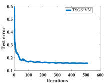
(a) CodRNA

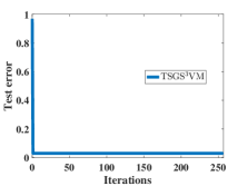
(b) W6a

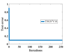
(c) IJCNN1

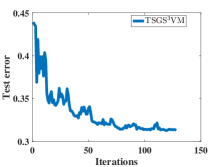
(d) SUSY

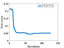
(e) Skin

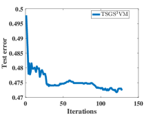
(f) Higgs

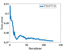
(g) Dota2

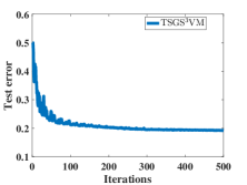
(h) HEPMASS

Figure 4: Test error of different S³VM solvers v.s. iterations on the eight benchmark data sets.

Appendix E Convergence curves related to iterations

We report the convergence curve related to iterations of TSGS³VM in Fig 4. Fig 4 shows that TSGS³VM usually converge to a good result in a few iterations (about 64-128). Note that, similar to DSG, our TSGS³VM implementation also uses a mini-batch setting, where the batch size is set to 256. Thus, in each iteration, TSGS³VM randomly sample 256 instances to compute the TSG.

References

• Bennett and Demiriz [1999] Kristin P Bennett and Ayhan Demiriz. Semi-supervised support vector machines. In Advances in Neural Information processing systems, pages 368–374, 1999.
• Cai and Cherkassky [2012] Feng Cai and Vladimir Cherkassky. Generalized smo algorithm for svm-based multitask learning. IEEE transactions on neural networks and learning systems, 23(6):997–1003, 2012.
• Carratino et al. [2018] Luigi Carratino, Alessandro Rudi, and Lorenzo Rosasco. Learning with sgd and random features. In Advances in Neural Information Processing Systems, pages 10213–10224, 2018.
• Chang and Lin [2011] Chih-Chung Chang and Chih-Jen Lin. LIBSVM: A library for support vector machines. ACM Transactions on Intelligent Systems and Technology, 2:27:1–27:27, 2011.
• Chapelle and Zien [2005] Olivier Chapelle and Alexander Zien. Semi-supervised classification by low density separation. In AISTATS, volume 2005, pages 57–64. Citeseer, 2005.
• Chapelle [2007] Olivier Chapelle. Training a support vector machine in the primal. Neural computation, 19(5):1155–1178, 2007.
• Collobert et al. [2006] Ronan Collobert, Fabian Sinz, Jason Weston, and Léon Bottou. Large scale transductive svms. Journal of Machine Learning Research, 7(Aug):1687–1712, 2006.
• Dai et al. [2014] Bo Dai, Bo Xie, Niao He, Yingyu Liang, Anant Raj, Maria-Florina F Balcan, and Le Song. Scalable kernel methods via doubly stochastic gradients. In Advances in Neural Information Processing Systems, pages 3041–3049, 2014.
• Drineas and Mahoney [2005] Petros Drineas and Michael W Mahoney. On the nyström method for approximating a gram matrix for improved kernel-based learning. journal of machine learning research, 6(Dec):2153–2175, 2005.
• Ghadimi and Lan [2013] Saeed Ghadimi and Guanghui Lan. Stochastic first-and zeroth-order methods for nonconvex stochastic programming. SIAM Journal on Optimization, 23(4):2341–2368, 2013.
• Gu et al. [2018a] Bin Gu, Zhouyuan Huo, Cheng Deng, and Heng Huang. Faster derivative-free stochastic algorithm for shared memory machines. In International Conference on Machine Learning, pages 1807–1816, 2018.
• Gu et al. [2018b] Bin Gu, Yingying Shan, Xiang Geng, and Guansheng Zheng. Accelerated asynchronous greedy coordinate descent algorithm for svms. In IJCAI, pages 2170–2176, 2018.
• Gu et al. [2018c] Bin Gu, Miao Xin, Zhouyuan Huo, and Heng Huang. Asynchronous doubly stochastic sparse kernel learning. In Thirty-Second AAAI Conference on Artificial Intelligence, 2018.
• Gu et al. [2018d] Bin Gu, Xiao-Tong Yuan, Songcan Chen, and Heng Huang. New incremental learning algorithm for semi-supervised support vector machine. In Proceedings of the 24th ACM SIGKDD International Conference on Knowledge Discovery & Data Mining, pages 1475–1484. ACM, 2018.
• Huo et al. [2018] Zhouyuan Huo, Bin Gu, and Heng Huang. Training neural networks using features replay. In Advances in Neural Information Processing Systems, pages 6659–6668, 2018.
• Joachims [1999] Thorsten Joachims. Transductive inference for text classification using support vector machines. In Icml, volume 99, pages 200–209, 1999.
• Le et al. [2016] Trung Le, Phuong Duong, Mi Dinh, Tu Dinh Nguyen, Vu Nguyen, and Dinh Q Phung. Budgeted semi-supervised support vector machine. In UAI, 2016.
• Li et al. [2017] Xiang Li, Bin Gu, Shuang Ao, Huaimin Wang, and Charles X Ling. Triply stochastic gradients on multiple kernel learning. In UAI, 2017.
• Lopez-Paz et al. [2014] David Lopez-Paz, Suvrit Sra, Alex Smola, Zoubin Ghahramani, and Bernhard Schölkopf. Randomized nonlinear component analysis. Computer Science, 4:1359–1367, 2014.
• Rahimi and Recht [2008] Ali Rahimi and Benjamin Recht. Random features for large-scale kernel machines. In Advances in neural information processing systems, pages 1177–1184, 2008.
• Reddi et al. [2016] Sashank J Reddi, Ahmed Hefny, Suvrit Sra, Barnabas Poczos, and Alex Smola. Stochastic variance reduction for nonconvex optimization. In International conference on machine learning, pages 314–323, 2016.
• Shi et al. [2019] Wanli Shi, Bin Gu, Xiang Li, Xiang Geng, and Heng Huang. Quadruply stochastic gradients for large scale nonlinear semi-supervised auc optimization. In 28th International Joint Conference on Artificial Intelligence, 2019.
• Wang et al. [2007] Junhui Wang, Xiaotong Shen, and Wei Pan. On transductive support vector machines. Contemporary Mathematics, 443:7–20, 2007.
• Wendland [2004] Holger Wendland. Scattered data approximation, volume 17. Cambridge university press, 2004.
• Xie et al. [2015] Bo Xie, Yingyu Liang, and Le Song. Scale up nonlinear component analysis with doubly stochastic gradients. In Advances in Neural Information Processing Systems, pages 2341–2349, 2015.
• Yu et al. [2019] Shuyang Yu, Bin Gu, Kunpeng Ning, Haiyan Chen, Jian Pei, and Heng Huang. Tackle balancing constraint for incremental semi-supervised support vector learning. In Proceedings of the 25th ACM SIGKDD International Conference on Knowledge Discovery & Data Mining, 2019.
• Yuille and Rangarajan [2002] Alan L Yuille and Anand Rangarajan. The concave-convex procedure (cccp). In Advances in neural information processing systems, pages 1033–1040, 2002.